Probabilistic Reach-Avoid for
Bayesian Neural Networks

Abstract

Model-based reinforcement learning seeks to simultaneously learn the dynamics of an unknown stochastic environment and synthesise an optimal policy for acting in it. Ensuring the safety and robustness of sequential decisions made through a policy in such an environment is a key challenge for policies intended for safety-critical scenarios. In this work, we investigate two complementary problems: first, computing reach-avoid probabilities for iterative predictions made with dynamical models, with dynamics described by Bayesian neural network (BNN); second, synthesising control policies that are optimal with respect to a given reach-avoid specification (reaching a “target” state, while avoiding a set of “unsafe” states) and a learned BNN model. Our solution leverages interval propagation and backward recursion techniques to compute lower bounds for the probability that a policy’s sequence of actions leads to satisfying the reach-avoid specification. Such computed lower bounds provide safety certification for the given policy and BNN model. We then introduce control synthesis algorithms to derive policies maximizing said lower bounds on the safety probability. We demonstrate the effectiveness of our method on a series of control benchmarks characterized by learned BNN dynamics models. On our most challenging benchmark, compared to purely data-driven policies the optimal synthesis algorithm is able to provide more than a four-fold increase in the number of certifiable states and more than a three-fold increase in the average guaranteed reach-avoid probability.

organization=Department of Computer Science, University of Oxford, Oxford, UK

organization=Delft Center for Systems and Control (DCSC), TU Delft, Delft, Netherlands

organization=Department of Informatics, King’s College London, London, UK

1 Introduction

The capacity of deep learning to approximate complex functions makes it particularly attractive for inferring process dynamics in control and reinforcement learning problems (Schrittwieser et al., 2019). In safety-critical scenarios where the environment and system state are only partially known or observable (e.g., a robot with noisy actuators/sensors), Bayesian models have recently been investigated as a safer alternative to standard, deterministic, Neural Networks (NNs): the uncertainty estimates of Bayesian models can be propagated through the system decision pipeline to enable safe decision making despite unknown system conditions (McAllister and Rasmussen, 2017; Carbone et al., 2020; Depeweg et al., 2017). In particular, Bayesian Neural Networks (BNNs) retain the same advantages of NNs (relative to their approximation capabilities) and also enable reasoning about uncertainty in a principled probabilistic manner (Neal, 2012; Murphy, 2012), making them very well-suited to tackle safety-critical problems.

In problems of sequential planning, time-series forecasting, and model-based reinforcement learning, evaluating a model with respect to a control policy (or strategy) requires making several predictions that are mutually dependent across time (Liang, 2005; Deisenroth and Rasmussen, 2011). While multiple models can be learned for each time step, a common setting is for these predictions to be made iteratively by the same machine learning model (Huang and Rosendo, 2020), where the state of the predicted model at each step is a function of the model state at the previous step and possibly of an action (from the policy). We refer to this setting as iterative predictions.

Unfortunately, performing iterative predictions with BNN models poses several practical issues. In facts, BNN models output probability distributions, so that at each successive timestep the BNN needs to be evaluated over a probability distribution, rather than a fixed input point – thus posing the problem of successive predictions over a stochastic input. Even when the posterior distribution of the BNN weights is inferred using analytical approximations, the deep and non-linear structure of the network makes the resulting predictive distribution analytically intractable (Neal, 2012). In iterative prediction settings, the problem is compounded and exacerbated by the fact that one would have to evaluate the BNN, sequentially, over a distribution that cannot be computed analytically (Depeweg et al., 2017). Hence, computing sound, formal bounds on the probability of BNN-based iterative predictions remains an open problem. Such bounds would enable one to provide safety guarantees over a given (or learned) control policy, which is a necessary precondition before deploying the policy in a real-world environment (Polymenakos et al., 2020; Vinogradska et al., 2016).

In this paper, we develop a new method for the computation of probabilistic guarantees for iterative predictions with BNNs over reach-avoid specifications. A reach-avoid specification, also known as constrained reachability (Soudjani and Abate, 2013), requires that the trajectories of a dynamical system reach a goal/target region over a given (finite) time horizon, whilst avoiding a given set of states that are deemed “unsafe”. Probabilistic reach-avoid is a key property for the formal analysis of stochastic processes (Abate et al., 2008), underpinning richer temporal logic specifications: its computation is the key component for probabilistic model checking algorithms for various temporal logics such as PCTL, csLTL, or BLTL (Kwiatkowska et al., 2007; Cauchi et al., 2019).

Even though the exact computation of reach-avoid probabilities for iterative prediction with BNNs is in general not analytically possible, with our method, we can derive a guaranteed (conservative) lower bound by solving a backward iterative problem obtained via a discretisation of the state space. In particular, starting from the final time step and the goal region, we back-propagate the probability lower bounds for each discretised portion of the state space. This backwards reachability approach leverages recently developed bound propagation techniques for BNNs (Wicker et al., 2020). In addition to providing guarantees for a given policy, we also devise methods to synthesise policies that are maximally certifiable, i.e., that maximize the lower bound of the reach-avoid probability. We first describe a numerical solution that, by using dynamic programming, can synthesize policies that are maximally safe. Then, in order to improve the scalability of our approach, we present a method for synthesizing approximately optimal strategies parametrised as a neural network. While our method does not yet scale to state-of-the-art reinforcement learning environments, we are able to verify and synthesise challenging non-linear control case studies.

We validate the effectiveness of our certification and synthesis algorithms on a series of control benchmarks. Our certification algorithm is able to produce non-trivial safety guarantees for each system that we test. On each proposed benchmark, we also show how our synthesis algorithm results in actions whose safety is significantly more certifiable than policies derived via deep reinforcement learning. Specifically, in a challenging planar navigation benchmark, our synthesis method results in policies whose certified safety probabilities are eight to nine times higher than those for learned policies.

We further investigate how factors like the choice of approximate inference method, BNN architecture, and training methodology affect the quality of the synthesised policy. In summary, this paper makes the following contributions:

• We show how probabilistic reach-avoid for iterative predictions with BNNs can be formulated as the solution of a backward recursion.

• We present an efficient certification framework that produces a lower bound on probabilistic reach-avoid by relying on convex relaxations of the BNN model and said recursive problem definition.

• We present schemes for deriving a maximally certified policy (i.e., maximizing the lower bound on safety probability) with respect to a BNN and given reach-avoid specification.

• We evaluate our methodology on a set of control case studies to provide guarantees for learned and synthesized policies and conduct an empirical investigation of model-selection choices and their effect on the quality of policies synthesised by our method.

A previous version of this work (Wicker et al., 2021b) has been presented at the thirty-seventh Conference on Uncertainty in Artificial Intelligence. Compared to the conference paper, in this work, we introduce several new contributions. Specifically, compared to Wicker et al. (2021b) we present novel algorithms for the synthesis of control strategies based on both a numerical method and a neural network-based approach. Moreover, the experimental evaluation has been consistently extended, to include, among others, an analysis of the role of approximate inference and NN architecture on safety certification and synthesis, as well as an in-depth analysis of the scalability of our methods. Further discussion of related works can be found in Section 7.

2 Bayesian Neural Networks

In this work, we consider fully-connected neural network (NN) architectures $f^{w}:\mathbb{R}^{m}\to\mathbb{R}^{n}$ parametrised by a vector $w\in\mathbb{R}^{n_{w}}$ containing all the weights and biases of the network. Given a NN $f^{w}$ composed by $L$ layers, we denote by $f^{w,1},...,f^{w,L}$ the layers of $f^{w}$ and we have that $w=\big{(}\{W_{i}\}_{i=1}^{L}\big{)}\cup\big{(}\{b_{i}\}_{i=1}^{L}\big{)}$, where $W_{i}$ and $b_{i}$ represent weights and biases of the $i-$th layer of $f^{w}.$ For $x\in\mathbb{R}^{n}$ the output of layer $i\in\{1,...,L\}$ can be explicitly written as $f^{w,i}(x)=a(W_{i}f^{w,{i-1}}(x)+b_{i})$ with $f^{w,1}(x)=a(W_{1}x+b_{1})$, where $a:\mathbb{R}\to\mathbb{R}$ is the activation function. We assume that $a$ is a continuous monotonic function, which holds for the vast majority of activation functions used in practice such as sigmoid, ReLu, and tanh (Goodfellow et al., 2016). This guarantees that $f^{w}$ is a continuous function.

Bayesian Neural Networks (BNNs), denoted by $f^{\mathbf{w}}$, extend NNs by placing a prior distribution over the network parameters, $p_{\mathbf{w}}(w)$, with $\mathbf{w}$ being the vector of random variables associated to the parameter vector $w$. Given a dataset $\mathcal{D}$, training a BNN on $\mathcal{D}$ requires to compute posterior distribution, $p_{\mathbf{w}}(w|\mathcal{D}),$ which can be computed via Bayes’ rule (Neal, 2012). Unfortunately, because of the non-linearity introduced by the neural network architecture, the computation of the posterior is generally intractable. Hence, various approximation methods have been studied to perform inference with BNNs in practice. Among these methods, we consider Hamiltonian Monte Carlo (HMC) (Neal, 2012), and Variational Inference (VI) (Blundell et al., 2015). In our experimental evaluation in Section 6.3 we employ both HMC and VI.

Hamiltonian Monte Carlo (HMC)

HMC proceeds by defining a Markov chain whose invariant distribution is $p_{\mathbf{w}}(w|\mathcal{D}),$ and relies on Hamiltionian dynamics to speed up the exploration of the space. Differently from VI discussed below, HMC does not make any parametric assumptions on the form of the posterior distribution and is asymptotically correct. The result of HMC is a set of samples that approximates $p_{\mathbf{w}}(w|\mathcal{D})$. We refer interested readers to (Neal et al., 2011; Izmailov et al., 2021) for further details.

Variational Inference (VI)

VI proceeds by finding a Gaussian approximating distribution $q(w)\sim p_{\mathbf{w}}(w|\mathcal{D})$ in a trade-off between approximation accuracy and scalability. The core idea is that $q(w)$ depends on some hyperparameters that are then iteratively optimized by minimizing a divergence measure between $q(w)$ and $p_{\mathbf{w}}(w|\mathcal{D})$. Samples can then be efficiently extracted from $q(w)$. See (Khan and Rue, 2021; Blundell et al., 2015) for recent developments in variational inference in deep learning.

3 Problem Formulation

Given a trained BNN $f^{\mathbf{w}}$ we consider the following discrete-time stochastic process given by iterative predictions of the BNN:

$$\mathbf{x}_{k}=f^{\mathbf{w}}(\mathbf{x}_{k-1},\mathbf{u}_{k-1})+\mathbf{v}_{k},\quad\mathbf{u}_{k}=\pi_{k}(\mathbf{x}_{k}),\quad k\in\mathbb{N}_{>0},$$ (1)

where $\mathbf{x}_{k}$ is a random variable taking values in $\mathbb{R}^{n}$ modelling the state of System (1) at time $k$, $\mathbf{v}_{k}$ is a random variable modelling an additive noise term with stationary, zero-mean Gaussian distribution $\mathcal{N}(0,\sigma^{2}\cdot I),$ where $I$ is the identity matrix of size $n\times n$. $\mathbf{u}_{k}$ represents the action applied at time $k$, selected from a compact set $\mathcal{U}\subset\mathbb{R}^{c}$ by a (deterministic) feedback Markov strategy (a.k.a. policy, or controller) $\pi:\mathbb{R}^{n}\times\mathbb{N}\to\mathcal{U}$.

The model in Eqn. (1) is commonly employed to represent noisy dynamical models driven by a BNN and controlled by the policy $\pi$ (Depeweg et al., 2017). In this setting, $f^{\mathbf{w}}$ defines the transition probabilities of the model and, correspondingly, $p(\bar{x}|(x,u),\mathcal{D})$ is employed to describe the posterior predictive distribution, namely the probability density of the model state at the next time step being $\bar{x}$, given that the current state and action are $(x,u)$, as:

$$p(\bar{x}|(x,u),\mathcal{D})=\int_{\mathbb{R}^{n_{w}}}\mathcal{N}(\bar{x}\mid f^{w}(x,u),\sigma^{2}\cdot I)p_{\mathbf{w}}(w|\mathcal{D})dw,$$ (2)

where $\mathcal{N}(\cdot\mid f^{w}(x,u),\sigma^{2}\cdot I)$ is the Gaussian likelihood induced by noise $\mathbf{v}_{k}$ and centered at the NN output (Neal, 2012).

Observe that the posterior predictive distribution induces a probability density function over the state space. In iterative prediction settings, this implies that at each step the state vector $\mathbf{x}_{k}$ fed into the BNN is a random variable. Hence, a $N$-step trajectory of the dynamic model in Eqn (1) is a sequence of states $x_{0},...,x_{N}\in\mathbb{R}^{n}$ sampled from the predictive distribution. As a consequence, a principled propagation of the BNN uncertainty through consecutive time steps poses the problem of predictions over stochastic inputs. In Section 4.1 we will tackle this problem for the particular case of reach-avoid properties, by designing a backward computation scheme that starts its calculations from the goal region, and proceeds according to Bellman iterations (Bertsekas and Shreve, 2004).

We remark that $p(\bar{x}|(x,u),\mathcal{D})$ is defined by marginalizing over $p_{\mathbf{w}}(w|\mathcal{D})$, hence, the particular $p(\bar{x}|(x,u),\mathcal{D})$ depends on the specific approximate inference method employed to estimate the posterior distribution. As such, the results that we derive are valid w.r.t. a specific BNN posterior.

Probability Measure

For an action $u\in\mathbb{R}^{c}$, a subset of states $X\subseteq\mathbb{R}^{n}$ and a starting state $x\in\mathbb{R}^{n}$, we call $T(X|x,u)$ the stochastic kernel associated (and equivalent (Abate et al., 2008)) to the dynamical model of Equation (1). Namely, $T(X|x,u)$ describes the one-step transition probability of the model of Eqn. (1) and is defined by integrating the predictive posterior distribution with input $(x,u)$ over $X$, as:

$$T(X|x,u)= \int_{X}p(\bar{x}|(x,u),\mathcal{D})d\bar{x}.$$ (3)

In what follows, it will be convenient at times to work over the space of parameters of the BNN. To do so, we can re-write the stochastic kernel by combining Equations (2) and (3) and applying Fubini’s theorem (Fubini, 1907) to switch the integration order, thus obtaining:

$$T(X|x,u)=\int_{\mathbb{R}^{n_{w}}}\left[\int_{X}\mathcal{N}(\bar{x}|f^{w}(x,u),\sigma^{2}\cdot I)d\bar{x}\right]p_{\mathbf{w}}(w|\mathcal{D})dw.$$ (4)

From this definition of $T$ it follows that, under a strategy $\pi$ and for a given initial condition $x_{0}$, $\mathbf{x}_{k}$ is a Markov process with a well-defined probability measure $\Pr$ uniquely generated by the stochastic kernel $T$ (Bertsekas and Shreve, 2004, Proposition 7.45) and such that for $X_{0},X_{k}\subseteq\mathbb{R}^{n}$:

$$\Pr[\mathbf{x}_{0}\in X_{0}]=\mathbf{1}_{X_{0}}(x_{0}),$$

$$\Pr[\mathbf{x}_{k}\in X_{k}|\mathbf{x}_{k-1}=x,\pi]=T(X_{k}|x,\pi_{k-1}(x)),$$

where $\mathbf{1}_{X_{0}}$ is the indicator function (that is, $1$ if $x\subseteq X_{0}$ and $0$ otherwise). Having a definition of $\Pr$ allows one to make probabilistic statements over the stochastic model in Eqn (1).

Remark 1

Note that, as is common in the literature (Depeweg et al., 2017), according to the definition of the probability measure $\Pr$ we marginalise over the posterior distribution at each time step. Consequently, according to our modelling framework, the weights of the BNN are not kept fixed during each trajectory, but we re-sample from $\mathbf{w}$ at each time step.

3.1 Problem Statements

We consider two problems concerning, respectively, the certification and the control of dynamical systems modelled by BNNs. We first consider safety certification with respect to probabilistic reach-avoid specifications. That is, we seek to compute the probability that from a given state, under a selected control policy, an agent navigates to the goal region without encountering any unsafe states. Next, we consider the formal synthesis of policies that maximise this probability and thus attain maximal certifiable safety.

Problem 1 (Computation of Probabilistic Reach-Avoid)

Given a strategy $\pi$, a goal region $\mathrm{G}\subseteq\mathbb{R}^{n}$, a finite-time horizon $[0,N]\subseteq\mathbb{N},$ and a safe set $\mathrm{S}\subseteq\mathbb{R}^{n}$ such that $\mathrm{G}\cap\mathrm{S}=\emptyset$, compute for any $x_{0}\in\mathrm{G}\cup\mathrm{S}$

$$P_{reach}(\mathrm{G},\mathrm{S},x_{0},[0,N]|\pi)=$$

$$\hskip 28.45274pt\Pr\big{[}\exists k\in[0,N],\mathbf{x}_{k}\in\mathrm{G}\,\wedge\forall 0\leq k^{\prime}<k,\mathbf{x}_{k^{\prime}}\in\mathrm{S}\mid\mathbf{x}_{0}=x_{0},\pi\big{]}.$$ (5)

Outline of the Approach

In Section 4.1 we show how $P_{reach}(\mathrm{G},\mathrm{S},x_{0},[0,N]|\pi)$ can be formulated as the solution of a backward iterative computational procedure, where the uncertainty of the BNN is propagated backward in time, starting from the goal region. Our approach allows us to compute a sound lower bound on $P_{reach}$, thus guaranteeing that $\mathbf{x}_{k},$ as defined in Eqn (1), satisfies the specification with a given probability. This is achieved by extending existing lower bounding techniques developed to certify BNNs (Wicker et al., 2020) and applying these at each propagation step through the BNN.

Note that, in Problem 1, the strategy $\pi$ is provided, and the goal is to quantify the probability with which the trajectories of $\mathbf{x}_{k}$ satisfy the given specification. In Problem 2 below, we expand the previous problem and seek to synthesise a controller $\pi$ that maximizes $P_{reach}$. The general formulation of this optimization is given below.

Problem 2 (Strategy Synthesis for Probabilistic Reach-Avoid)

For an initial state $x_{0}\in\mathrm{G}\cup\mathrm{S}$, and a finite time horizon $N$, find a strategy $\pi^{*}:\mathbb{R}^{n}\times\mathbb{R}_{\geq 0}\to\mathbb{R}^{c}$ such that

$$\pi^{*}=\operatorname*{arg\,max}_{\pi}P_{reach}(\mathrm{G},\mathrm{S},x_{0},[0,N]\mid\pi).$$ (6)

In Section 5, we will provide specific schemes for synthesizing optimal strategies when $\pi$ is either a look-up table or a deterministic neural network.

Outline of the Approach

To solve this problem, we notice that the backward iterative procedure outlined to solve Problem 1 has a substructure such that dynamic programming will allow us to compute optimal actions for each state that we verify, thus producing an optimal policy with respect to the given posterior and reach-avoid specification. With low-dimensional or discrete action spaces, we can then derive a tabular policy by solving the resulting dynamic programming problem. For higher-dimensional action spaces instead, in Section 5.1 we consider (generalising) policies represented as neural networks.

4 Methodology

In this section, we illustrate the methodology used to compute lower bounds on the reach-avoid probability, as described in Problem 1. We begin by encoding the reach-avoid probability through a sequence of value functions.

4.1 Certifying Reach-Avoid Specifications

We begin by showing that $P_{reach}(\mathrm{G},\mathrm{S},x,[k,N]|\pi)$ can be obtained as the solution of a backward iterative procedure, which allows to compute a lower bound on its value. In particular, given a time $0\leq k<N$ and a strategy $\pi,$ consider the value functions $V_{k}^{\pi}:\mathbb{R}^{n}\to[0,1]$, recursively defined as

$$V_{N}^{\pi}(x)=\mathbf{1}_{\mathrm{G}}(x),$$

$$V_{k}^{\pi}(x)=\mathbf{1}_{\mathrm{G}}(x)+\mathbf{1}_{\mathrm{S}}(x){\int V^{\pi}_{k+1}(\bar{x})p\big{(}\bar{x}|(x,\pi_{k}(x)),\mathcal{D}\big{)}d\bar{x}}.$$ (7)

Intuitively, $V_{k}^{\pi}$ is computed starting from the goal region $\mathrm{G}$ at $k=N$, where it is initialised at value $1$. The computation proceeds backwards at each state $x$, by combining the current values with the transition probabilities from Eqn (1). The following proposition, proved inductively over time in the Supplementary Material, guarantees that $V_{0}^{\pi}(x)$ is indeed equal to $P_{reach}(\mathrm{G},\mathrm{S},x,[0,N]|\pi)$.

Proposition 1

For $0\leq k\leq N$ and $x_{0}\in\mathrm{G}\cup\mathrm{S},$ it holds that

$$P_{reach}(\mathrm{G},\mathrm{S},x_{0},[k,N]|\pi)=V_{k}^{\pi}(x).$$

The backward recursion in Eqn (7) does not generally admit a solution in closed-form, as it would require integrating over the BNN posterior predictive distribution, which is in general analytically intractable. In the following section, we present a computational scheme utilizing convex relaxations to lower bound $P_{reach}$.

Figure 1: Examples of functions $K^{\pi}_{N-1}$ (left) and $K^{\pi}_{N-2}$ (right), which are lower bounds of $V^{\pi}_{k}$. On the left, we consider the first step of our backward algorithm, where we compute $K^{\pi}_{N-2}(q)$ by computing the probability that $\mathbf{x}_{N}\in\mathrm{G}$ given that $\mathbf{x}_{N-1}\in q.$ On the right, we consider the subsequent step. We outline the state we want to verify in red and the goal region in green. With the orange arrow, we represent the 0.95 transition probability of the BNN dynamical model, and in pink we represent the worst-case probabilities spanned by the BNN output. On top, we show where each of these key terms comes into play in Eqn (9).

4.2 Lower Bound on $P_{reach}$

We develop a computational approach based on the discretisation of the state space, which allows convex relaxation methods such as (Wicker et al., 2020) to be used. The proposed computational approach is illustrated in Figure 1 and formalized in Section 4.3. Let $Q=\{q_{1},...,q_{n_{q}}\}$ be a partition of $\mathrm{S}\cup\mathrm{G}$ in $n_{q}$ regions and denote with $z:\mathbb{R}^{n}\to Q$ the function that associates to a state in $\mathbb{R}^{n}$ the corresponding partitioned state in $Q$. For each $0\leq k\leq N$ we iteratively build a set of functions $K^{\pi}_{k}:Q\rightarrow[0,1]$ such that for all $x\in\mathrm{G}\cup\mathrm{S}$ we have that $K^{\pi}_{k}(z(x))\leq V^{\pi}_{k}(x)$. Intuitively, $K^{\pi}_{k}$ provides a lower bound for the value functions on the computation of $P_{reach}$.

The functions $K^{\pi}_{k}$ are obtained by propagating backward the BNN predictions from time $N$, where we set $K^{\pi}_{N}(q)=\mathbf{1}_{\mathrm{G}}(q)$, with $\mathbf{1}_{\mathrm{G}}(q)$ being the indicator function (that is, $1$ if $q\subseteq\mathrm{G}$ and $0$ otherwise). Then, for each $k<N$, we first discretize the set of possible probabilities in $n_{p}$ sub-intervals $0=v_{0}\leq v_{1}\leq...\leq v_{n_{p}}=1$. Hence, for any $q\in Q$ and probability interval $[v_{i},v_{i+1}]$, one can compute a lower bound, $R(q,k,\pi,i)$, on the probability that, starting from any state in $q$ at time $k$, we reach in the next step a region that has probability $\in[v_{i},v_{i+1}]$ of safely reaching the goal region. The resulting values are used to build $K^{\pi}_{k}$ (as we will detail in Eqn (9)). For a given $q\subset\mathrm{S}$, $K^{\pi}_{k}(q)$ is obtained as the sum over $i$ of $R(q,k,\pi,i)$ multiplied by $v_{i-1}$, i.e., the lower value that $K^{\pi}_{k+1}$ obtains in all the states of the $i-th$ region. Note that the discretisation of the probability values does not have to be uniform, but can be adaptive for each $q\in Q$. A heuristic for picking the value of thresholds $v_{i}$ will be given in Algorithm 1. In what follows, we formalise the intuition behind this computational procedure.

4.3 Lower Bounding of the Value Functions

For a given strategy $\pi$, we consider a constant $\eta\in(0,1)$ and $\epsilon=\sqrt{2\sigma^{2}}\text{erf}^{-1}(\eta)$, which are used to bound the value of the noise, $\mathbf{v}_{k}$, at any given time. Intuitively, $\eta$ represents the proportion of observational error we consider. Then, for $0\leq k<N$, $K^{\pi}_{k}:Q\to[0,1]$ are defined recursively as follows:

$$K^{\pi}_{N}(q)=\mathbf{1}_{\mathrm{G}}(q),$$ (8)

$$K^{\pi}_{k}(q)=\mathbf{1}_{\mathrm{G}}(q)+\mathbf{1}_{\mathrm{S}}(q)\sum_{i=1}^{n_{p}}v_{i-1}R(q,k,\pi(q),i),$$ (9)

where

$$R(q,k,\pi(q),i)=\eta^{n}\int_{H^{q,\pi,\epsilon}_{k,i}}p_{\mathbf{w}}(w|\mathcal{D})dw,$$ (10)

$$H^{q,\pi,\epsilon}_{k,i}=\{w\in\mathbb{R}^{n_{w}}|\,\forall x\in q,\forall\gamma\in[-\epsilon,\epsilon]^{n},\text{ it holds that: }$$

$$\hskip 8.5359ptv_{i-1}\leq K_{k+1}^{\pi}(q^{\prime})\leq v_{i},\text{ with $q^{\prime}=z(f^{w}(x,\pi_{k}(x))+\gamma)$}\}.$$

The key component for the above backward recursion is $R(q,k,\pi,i)$, which bounds the probability that, starting from $q$ at time $k$, we have that $\mathbf{x}_{k+1}$ will be in a region $q^{\prime}$ such that $K_{k+1}^{\pi}(q^{\prime})\in[v_{i},v_{i+1}]$. By definition, the set $H^{q,\pi,\epsilon}_{k,i}$ defines the weights for which the BNN maps all states covered by $q$ into the goal states given action $\pi(q)$. Given this, it is clear that integration of the posterior $p_{\mathbf{w}}(w|\mathcal{D})$ over the $H^{q,\pi,\epsilon}_{k,i}$ will return the probability mass of system (1) transitioning from $q$ to $q^{\prime}$ with probability in $[v_{i},v_{i+1}]$ in one time step. The computation of Eqn (9) then reduces to computing the set of weights $H^{q,\pi,\epsilon}_{k,i}$, which we call the projecting weight set. A method to compute a safe under-approximation $\bar{H}\subseteq H^{q,\pi,\epsilon}_{k,i}$ is discussed below. Before describing that, we analyze the correctness of the above recursion.

Theorem 1

Given $x\in\mathbb{R}^{n}$, for any $k\in\{0,...,N\}$ and $q=z(x)$, assume that $H^{q,\pi,\epsilon}_{k,i}\cap H^{q,\pi,\epsilon}_{k,j}=\emptyset$ for $i\neq j.$ Then:

$$\inf_{x\in q}V_{k}^{\pi}(x)\geq K^{\pi}_{k}(q).$$

A proof of Theorem 1 is given in the Supplementary Material. Note that the assumption on the null intersection between different projecting weight sets required in Theorem 1 can always be enforced by taking their intersection and complement.

4.4 Computation of Projecting Weight Set

Theorem 1 allows us to compute a safe lower bound to Problem 1, by relying on an abstraction of the state space, that is, through the computation of $K^{\pi}_{0}(q)$. This can be evaluated once the projecting set of weight values $H^{q,\pi,\epsilon}_{k,i}$ associated to $[v_{i-1},v_{i}]$ is known. Unfortunately, direct computation of $H^{q,\pi,\epsilon}_{k,i}$ is intractable. Nevertheless, a method for its lower bounding was developed by Wicker et al. (2020) in the context of adversarial perturbations for one-step BNN predictions, and can be directly adapted to our settings.

The idea is that an under approximation $\bar{H}\subseteq H^{q,\pi,\epsilon}_{k,i}$ is built by sampling weight boxes of the shape $\hat{H}=[w^{L},w^{U}]$, according to the posterior, and checking whether:

$$v_{i-1}\leq K_{k+1}^{\pi}(z(f^{w}({x},\pi_{k}(x))+\gamma))\leq v_{i},$$

$$\forall x\in q,\,\forall w\in\hat{H},\,\forall\gamma\in[-\epsilon,\epsilon]^{n}.$$ (11)

Finally, $\bar{H}$ is built as a disjoint union of boxes $\hat{H}$ satisfying the above condition. For a full discussion of the details of this method we refer interested readers to (Wicker et al., 2020). In order to apply this method to our setting, we propagate the abstract state $q$ through the policy function $\pi_{k}(x)$, so as to obtain a bounding box $\widehat{\Pi}=[\pi^{L},\pi^{U}]$ such that $\pi^{L}\leq\pi_{k}(x)\leq\pi^{U}$ for all $x\in q$. In the experiments, this bounding is only necessary when $\pi_{k}(x)$ is given by an NN controller, for which bound propagation of NNs can be used for the computation of $\widehat{\Pi}$ (Gowal et al., 2018; Gehr et al., 2018).

The results of Proposition 2 and Proposition 3 from Wicker et al. (2020) can then be used to propagate $q$, $\widehat{\Pi}$ and $\hat{H}$ through the BNN. For discrete posteriors (e.g., those resulting from HMC) one can use the method described by Gowal et al. (2018) (Equations 6 and 7). Propagation of $q$, $\widehat{\Pi}$ amounts to using these method to compute values $f^{L}_{q,\epsilon,k}$ and $f^{U}_{q,\epsilon,k}$ such that, for all $x\in q,\gamma\in[-\epsilon,\epsilon]^{n},w\in\hat{H}$, it holds that:

$$f^{L}_{q,\epsilon,k}\leq f^{w}({x},\pi_{k}(x))+\gamma\leq f^{U}_{q,\epsilon,k}.$$ (12)

Furthermore, $f^{L}_{q,\epsilon,k}$ and $f^{U}_{q,\epsilon,k}$ are differentiable w.r.t. to the input vector (Gowal et al., 2018; Wicker et al., 2021a).

Finally, the two bounding values can be used to check whether or not the condition in Eqn (11) is satisfied, by simply checking whether $[f^{L}_{q,\epsilon,k},f^{U}_{q,\epsilon,k}]$ propagated through $K_{k+1}^{\pi}$ is within $[v_{i},v_{i+1}]$. We highlight that computing this probability is equivalent to a conservative estimate of $R(q,k,\pi,i)$.

4.5 Probabilistic Reach-Avoid Algorithm

In Algorithm 1 we summarize our approach for computing a lower bound for Problem 1. For simplicity of presentation, we consider the case $n_{p}=2$, (i.e., we partition the range of probabilities in just two intervals $[0,v_{1}],$ $[v_{1},1]$ - the case $n_{p}>2$ follows similarly). The algorithm proceeds by first initializing the reach-avoid probability for the partitioned states $q$ inside the goal region $G$ to $1$, as per Eqn (8). Then, for each of the $N$ time steps and for each one of the remaining abstract states $q$, in line $4$ we set the threshold probability $v_{1}$ equal to the maximum value that $K^{\pi}$ attains at the next time step over the states in the neighbourhood of $q$ (which we capture with a hyper-parameter $\rho_{x}>0$). We found this heuristic for the choice of $v_{1}$ to work well in practice (notice that the obtained bound is formal irrespective of the choice of $v_{1}$, and different choices could potentially be explored). We then proceed in the computation of Eqn (9). This computation is performed in lines $5$–$14$. First, we initialise to the null set the current under-approximation of the projecting weight set, $\bar{H}$. We then sample $n_{s}$ weights boxes $\hat{H}$ by sampling weights from the posterior, and expanding them with a margin $\rho_{w}$ heuristically selected (lines 6-8). Then, for each of these sets, we first propagate the state $q$, policy function, and weight set $\bar{H}$ to build a box $\bar{X}$ according to Eqn (12) (line 9), which is then accepted or rejected based on the value that $K^{\pi}$ at the next time step attains in states in $\bar{X}$ (lines 10-12). $K^{\pi}_{N-i}(q)$ is then computed in line 14 by integrating $p_{\mathbf{w}}(w|\mathcal{D})$ over the union of the accepted sets of weights.

Algorithm 1 Probabilistic Reach-Avoid for BNNs

Input: BNN model $f^{\mathbf{w}}$, safe region $\mathrm{S}$, goal region $\mathrm{G}$, discretization $Q$ of $\mathrm{S}\cup\mathrm{G}$, time horizon $N$, neural controller $\pi$, number of BNN samples $n_{s}$, weight margin $\rho_{w}$, state space margin $\rho_{x}$
Output: Lower bound on $V^{\pi}$

1:For all $0\leq k\leq N$ set $K^{\pi}_{k}(q)=1$ iff $q\subseteq\mathrm{G}$ and $0$ otherwise

2:for $k\leftarrow N$ to $1$ do

3:   for $q\in Q\setminus\mathrm{G}$ do

4:      $v_{1}\leftarrow\max_{x\in[q-\rho_{x},q+\rho_{x}]}K^{\pi}_{k+1}(z(x))$

5:      $\bar{H}\leftarrow\emptyset$     # $\bar{H}$ is the set of safe weights

6:      for desired number of samples, $n_{s}$ do

7:         $w^{\prime}\sim P(w|\mathcal{D})$

8:         $\hat{H}\leftarrow[w^{\prime}-\rho_{w},w^{\prime}+\rho_{w}]$

9:         $\bar{X}\leftarrow[f^{L}_{q,\epsilon,k},f^{U}_{q,\epsilon,k}]\quad$ # Computed according to Eqn (12)

10:         if $\min_{x\in\bar{X}}K^{\pi}_{k+1}(z(x))\geq v_{1}$ then

11:           $\bar{H}\leftarrow\bar{H}\bigcup\hat{H}$

12:         end if

13:      end for

14:      Ensure $H_{i}\cap H_{j}=\emptyset\quad\forall H_{i},H_{j}\in\bar{H}$

15:      $K^{\pi}_{k}(q)=v_{1}\cdot\eta^{n}\int_{\bar{H}}p_{\mathbf{w}}(w|\mathcal{D})dw$   (Eqn (9))

16:   end for

17:end for

18:return $K^{\pi}$

5 Strategy Synthesis

We now focus on synthesising a strategy that maximizes our lower bound on $P_{reach}$, thus solving Problem 2. Notice that, while no global optimality claim can be made about the strategy that we obtain, maximising the lower bound guarantees that the true reach-avoid probability will still be greater than the improved bound obtained after the maximisation.

Definition 1

A strategy $\pi^{*}$ is called maximally certified (max-cert), w.r.t. the discretised value function $K^{\pi}$, if and only if, for all $x\in\mathrm{G}\cup\mathrm{S}$, it satisfies

$$K_{0}^{\pi^{*}}(z(x))=\sup_{\pi}K_{0}^{\pi}(z(x)),$$

that is, the strategy $\pi^{*}$ maximises the lower bound of $P_{reach}$.

It follows that, if $K_{0}^{\pi^{*}}(z(x))>1-\delta$ for all $x\in\mathrm{G}\cup\mathrm{S}$, then the max-cert strategy $\pi^{*}$ is a solution of Problem 2. Note that a max-cert strategy is guaranteed to exist when the set of admissible controls $\mathcal{U}$ is compact (Bertsekas and Shreve, 2004, Lemma 3.1), as we assume in this work. In the next theorem, we show that a max-cert strategy can be computed via dynamic programming with a backward recursion similar to that of Eqn (9).

Theorem 2

For $0\leq k<N$ and $0=v_{0}<...<v_{n_{p}}=1,$ define the functions $K^{*}_{k}:\mathbb{R}^{n}\to[0,1]$ recursively as follows

$$K^{*}_{k}(q)=\sup_{u\in\mathcal{U}}\big{(}\mathbf{1}_{\mathrm{G}}(q)+\mathbf{1}_{\mathrm{S}}(q)\sum_{i=1}^{n_{p}}v_{i}R(q,k,u,i)\big{)},$$

where $R(q,k,u,i)$ and $H^{q,u,\epsilon}_{k,i}$ are defined as in Eqn (10). If $\pi^{*}$ is s.t. $K^{*}_{0}=K^{\pi^{*}}_{0}$, then $\pi^{*}$ is a max-cert strategy. Furthermore, for any $x$, it holds that $K^{\pi^{*}}_{0}(z(x))\leq P_{reach}(\mathrm{G},\mathrm{S},[0,N],x|\pi^{*})$.

Theorem 2 is a direct consequence of the Bellman principle of optimality (Abate et al., 2008, Theorem 2) and it guarantees that for each state $q\in\mathrm{S}$ and time $k$, we have that $\pi^{*}(q,k)=\text{arg}\max_{u\in\mathcal{U}}\sum_{i=1}^{n_{p}}v_{i}R(q,k,u,i).$

In Algorithm 2 we present a numerical scheme based on Theorem 2 to find a max-cert policy $\pi^{*}$. Note that the optimization problem required to be solved at each time step state, i.e. $\text{arg}\max_{u\in\mathcal{U}}\sum_{i=1}^{n_{p}}v_{i}R(q,k,u,i),$ is non-convex. Hence, in Algorithm 2, in Line 1, we start by partitioning the action space $\mathcal{U}$. Then, in Lines 4–15 for each action in the partition we estimate the expectation of $K^{*}_{k+1}$ starting from $q$ via $n_{s}$ samples taken from the BNN posterior (250 in all our experiments). Finally, in Lines 11–14 we keep track of the action maximising $K^{*}_{k+1}$.

The described approach for synthesis, while optimal in the limit of an infinitesimal discretization of $\mathcal{U}$, may become infeasible for large state and action spaces. As a consequence, in the next subsection, we also consider when $\pi$ is parametrised by a neural network and thus can serve as a function over a larger (even infinite) state space. Specifically, we show how a set of neural controllers, one for each time step, can be trained in order to maximize probabilistic reach-avoid via Theorem 2. In Section 6 we empirically investigate both controller strategies.

Algorithm 2 Numerical Synthesis of Action for region $q$ at time $k$

Input: BNN model $f^{\mathbf{w}}$, safe region $\mathrm{S}$, goal region $\mathrm{G}$, action space $\mathcal{U}$, abstract state $q\in Q$, controller $\pi$, number of BNN samples $n_{s}$
Output: Action maximizing $K^{\pi}$

1:$\Upsilon\leftarrow$ middle points of each region in a partition of $\mathcal{U}$

2:$\kappa^{*}\leftarrow 0$

3:$u^{*}\leftarrow 0$

4:for $u\in\Upsilon$ do

5:   $\hat{\kappa}\leftarrow 0$

6:   for $j$ from $0$ to $n_{s}$ do

7:      $w^{\prime}\sim P(w|\mathcal{D})$

8:      $\bar{X}\leftarrow[f^{L}_{q,\epsilon,k},f^{U}_{q,\epsilon,k}]$ # Computed for $q$ and $u$ via $(\text{Eqn \eqref{eq:ibp_final_results})}$

9:      $\hat{\kappa}=\hat{\kappa}+\frac{\min_{x\in\bar{X}}K^{*}_{k+1}(z(x))}{n_{s}}$

10:   end for

11:   if $\hat{\kappa}>\kappa^{*}$ then

12:      $\kappa^{*}\leftarrow\hat{\kappa}$

13:      $u^{*}\leftarrow u$

14:   end if

15:end for

16:return $u^{*}$

5.1 An Approach for Strategy Synthesis Based on Neural Networks

In this subsection we show how we can train a set of NN policies $\pi_{0},...,\pi_{N-1}:\mathbb{R}^{n}\to\mathcal{U}$ such that at each time step $k$, $\pi_{k}$ approximately solves the dynamic programming equation in Theorem 2. Note that, because of the approximate nature of the NN training, the resulting neural policies will necessarily be sub-optimal, but have the potential to scale to larger and more complex systems, compared to the approach presented in Algorithm 2.

At time $k$ we start with an initial set of parameters (weights and biases) $\theta_{k}$ for policy $\pi_{k}$. These parameters can either be initialized to ${\theta_{k+1}}$, the parameters synthesised at the previous time step of the value iteration for $\pi_{k+1}$, or to a policy employed to collect the data to train the BNN as in Gal et al. (2016b), or simply selected at random. In our implementation where no previous policy is available, we start with a randomly initialized NN, and then at time $k$ we set our initial neural policy with that obtained at time $k+1$. We then employ a scheme to learn a “safer” set of parameters via backpropagation. In particular, we first define the following loss function penalizing policy parameters that lead to an unsafe behavior for an ensemble of NNs sampled from the BNN posterior distribution:

$$\mathcal{L}(x,\theta_{k})=-\alpha||\sum_{w\in\bar{W}}f^{w}(x,\pi_{k}(x))-\mathbf{A}_{k}||_{2}+(1-\alpha)||\sum_{w\in\bar{W}}f^{w}(x,\pi_{k}(x))-\mathbf{R}_{k}||_{2},$$ (13)

where $\bar{W}$ are a set of parameters independently sampled from the BNN posterior $p_{\mathbf{w}}(w|\mathcal{D}),$ for a probability threshold $0\leq p_{t}\leq 1,$ $\mathbf{A}_{k}=\{x:K^{\pi_{{k+1}}}_{k+1}(x)\geq p_{t}\}$ and $\mathbf{R}_{k}=\{x:K^{\pi_{{k+1}}}_{k+1}(x)\leq 1-p_{t}\}$ are the sets of states for which the probability of satisfying the specification at time $k+1$ is respectively greater than $p_{t}$ and smaller than $1-p_{t}$. For $X\subset\mathbb{R}^{n},$ $||x-X||_{2}=\inf_{\bar{x}\in X}||x-\bar{x}||_{2}$ is the standard $L_{2}$ distance of a point from a set, and $0\leq\alpha\leq 1$ is a parameter taken to be 0.25 in our experiments, that weights between reaching the goal and staying away from “bad” states. Intuitively, the first term in $\mathcal{L}(x,\theta_{k})$ enforces $\theta_{k}$ that leads to high values of $K^{\pi_{{k+1}}}_{k+1}$, while the second term penalizes parameter sets that lead to small values of this quantity.

$\mathcal{L}(x,\theta_{k})$ only considers the behaviour of the dynamical system of Equation (1) starting from initial state $x$. Then, in order to also enforce robustness in a neighbourhood of initial states around $x$, similarly to the adversarial training case (Madry et al., 2017), we consider the robust loss

$$\bar{\mathcal{L}}(x,\theta_{k})=\max_{x^{\prime}:||x-x^{\prime}||_{2}\leq\epsilon}\mathcal{L}(x,\theta_{k}),$$ (14)

Note that by employing Eqn (12) we obtain a differentiable upper bound of $\bar{\mathcal{L}}(x,\theta_{k})$, which can be employed for training $\theta_{k}$.

5.2 Discussion on the Algorithms

In this section we provide further discussion of our proposed algorithms including the complexity and the various sources of approximation that may lead to looser guarantees. To frame this discussion, we start by highlighting the complexity and approximation introduced by the chosen bound propagation technique shared by both of the algorithms. We then proceed to discuss how discretisation choices made with respect to the state-space, the weight-space, and the observational noise, practically affect the tightness of our probability bounds for both algorithms, and finally how the action-space discretisation affects our synthesis algorithm.

Bound Propagation Techniques

Given that there are currently no methods for BNN certification that are both sound and complete (Wicker et al., 2020, 2021b; Berrada et al., 2021), the evaluation of the $R$ function will always introduce some approximation error. While it is difficult to characterize this error in general, it is known that for deeper networks, BNN certification methods introduce more approximation than shallow networks (Wicker, 2021). The recently developed bounds from Berrada et al. (2021), have been shown to be tighter than the IBP and LBP approaches from Wicker et al. (2020) at the cost of computation complexity that is exponential in the number of dimensions of the state-space. In contrast, each iteration of the interval bound propagation method proposed in and Wicker et al. (2020) requires the computational complexity of four forward passes through the neural network architecture.

Discretization Error and Complexity

While our formulation supports any form of state space discretisation, we can assume for simplicity that each dimension of the $n$-dimensional state-space is broken into $m$ equal-sized abstract states. This implies that certification of the system requires us to evaluate the $R$ function $\mathcal{O}\big{(}N(m^{n})\big{)}$ many times, where $N$ is the time horizon we would like to verify. Given that $n$ is fixed, the user has control over $m$, the size of each abstract state. For large abstract states, small $m$, one introduces more approximation as the $R$ function must account for all possible behaviors in the abstract state. For small abstract states, large $m$, there is much less approximation, but considerably larger runtime. Assume the $c$-dimensional action space is broken into $t$ equal portions at each dimension, then the computational complexity of the algorithm becomes $\mathcal{O}\big{(}t^{c}N(m^{n})\big{)}$ as each of the $m^{n}$ states must be evaluated $t^{c}$-many times to determine the approximately optimal action. As with the state-space discretization, larger $t$ will lead to a more-optimal action choice but requires greater computational time.

6 Experiments

We provide an empirical analysis of our BNN certification and policy synthesis methods. We begin by providing details on the experimental setting in Section 6.1. We then analyse the performance of our certification approach on synthesized policies in Section 6.2. Next, in Section 6.3, we discuss how the choice of the BNN inference algorithm affects synthesis and certification results. Finally, in Section 6.4 we study how our method scales with larger neural network architectures and in higher-dimensional control settings.

6.1 Experimental Setting

We consider a planar control task consisting of a point-mass agent navigating through various obstacle layouts. The point-mass agent is described by four dimensions, two encoding position information and two encoding velocity (Astrom and Murray, 2008). To control the agent there are two continuous action dimensions, which represent the force applied on the point-mass in each of the two planar directions. The task of the agent is to navigate to a goal region while avoiding various obstacle layouts. The knowledge supplied to the agent about the environment is the locations of the goal and obstacles. The full set of equations describing the agent dynamics is given in A.1. In our experiments, we analyse three obstacle layouts of varying difficulty, which we name v1, v2 and Zigzag - visualized in the left column of Figure 3. Obstacle layout v1 places an obstacle directly between the agent’s initial position and the goal, forcing the agent to navigate its way around it. Obstacle layout v2 extends this setting by adding two further obstacles that block off one side of the state space. Finally, scenario Zigzag has 5 interleaving triangles and requires the agent to navigate around them in order to reach the goal.

In order to learn an initial policy to solve the task, we employ the episodic learning framework described in Gal et al. (2016a). This consists of iteratively collecting data from deploying our learned policy, updating the BNN dynamics model to the new observations, and updating our policy. When collecting data, we start by randomly sampling state-action pairs and observing their resulting state according to the ground-truth dynamics. After this initial sample, all future observations from the ground-truth environment are obtained from deploying our learned policy. The initial policy is set by assigning a random action to each abstract state. This is equivalent to tabular policy representations in standard reinforcement learning (Sutton and Barto, 1998). We additionally discuss neural network policies in Section 6.4. Actions in the policy are updated by performing gradient descent on a sum of discounted rewards over a pre-specified finite horizon. The reward of an action is taken to be the $\ell_{2}$ distance moved towards the goal region penalized by the $\ell_{2}$ proximity to obstacles as is done in (Sutton and Barto, 1998; Gal et al., 2016a). For the learning of the BNN, we perform approximate Bayesian inference over the neural network parameters. For our primary investigation, we select an NN architecture with a single fully connected hidden layer comprising 50 hidden units, and learn the parameters via Hamiltonian Monte Carlo (HMC). Larger neural network architectures are considered in Section 6.4, while results for variational approximate inference are given in Section 6.3.

Unless otherwise specified, in performing certification and synthesis we employ abstract states spanning a width of $0.02$ around each position dimension and $0.08$ around each velocity dimension. Velocity values are clipped to the range $[-0.5,0.1]$. When performing optimal synthesis, we discretise the two action dimensions for the point-mass problem into 100 possible vectors which uniformly cover the continuous space of actions $[-1,1]$. When running our backward reachability scheme, at each state, we test all 100 action vectors and take the action that maximizes our lower bound to be the policy action at that state, thus giving us the locally optimal action within the given discretisation. Further experimental details are presented in A and code to reproduce all results in this paper can be found at https://github.com/matthewwicker/BNNReachAvoid.

The computational times for each system were roughly equivalent. This is to be expected given that each has the same state space. The following average times are reported for a parallel implementation of our algorithm run on 90 logical CPU cores across 4 Intel Core Xeon 6230 clocked at 2.10GHz. Training of the initial policy and BNN model takes in the order of 10 minutes, 6 hours for the certification with a horizon of 50 time steps, and 8 hours for synthesis.

Figure 2: Left Column: 200 simulated trajectories for the learned policy starting from the initial state. Center Left Column: A 2D visualization of the learned policy. Each arrow represents the direction of the applied force. Center Right Column: The epistemic uncertainty for the learned dynamics model. Right Column: Certified lower-bounds of probabilistic reach avoid for each abstract state according to BNN and final learned policy.

6.2 Comparing Certification of Learned and Max-Cert Policies

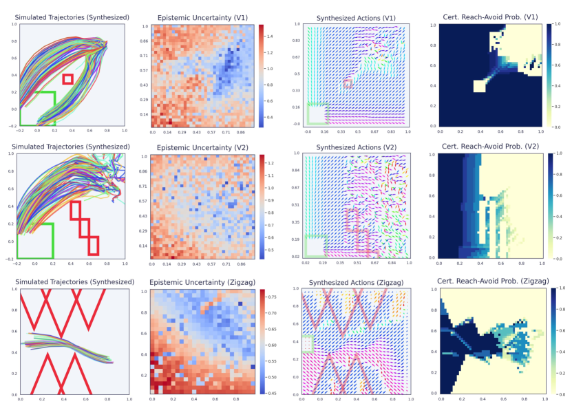
Figure 3: A version of each learned system after a new policy has been synthesized from the reach-avoid specification. First column: 200 simulations of the synthesized policy in the real environment. Second column: BNN epistemic uncertainty given as the variance of the BNN predictive distribution. Third column: A visualization of the maximally certifiable policies, which demonstrate a clearer tendency to avoid obstacles throughout the state space compared to the policies in Figure 2. Fourth column: Synthesized policies have remarkably higher lower-bounds than learned policies, corresponding plots for learned systems in Figure 2.

In Figure 2 and Figure 3 we visualize systems from both learned and synthesized policies. Each row represents one of our control environments and is comprised of four figures. These figures show, respectively, simulations from the dynamical system, BNN uncertainty, the control policy plotted as a gradient field, and the certified safety probabilities. The first column of the Figures depicts 200 simulated trajectories of the learned (Figure 2) or synthesized (Figure 3) control policies on the BNN (whose uncertainty is plotted along the second column). Notice how in both cases we visually obtain the behaviour expected, with the overwhelming majority of the simulated trajectories safely avoiding the obstacles (red regions in the figure) and terminating in the goal (green region). A vector field associated with the policy is depicted in the third column of the figures. Notice that, the actions returned by our synthesis method intuitively align with the reach-avoid specification, that is, synthesized actions near the obstacle and out-of-bounds are aligned with moving away from such unsafe states. Exceptions to this are represented by locations where the agent is already unsafe and that, as such, are not fully explored during the BNN learning phase (e.g., the lower triangles in the Zigzag scenario), locations where two directions are equally optimal (e.g., in the top right corner of the v1 environment) and locations which are not along any feasibly optimal path (e.g., the lower right corner of v2) and as such are not accounted by the BNN learning.

In Table 1 we compare the certification results of the synthesized policy against the initial learned policy. As the synthesized policy is computed by improving on the latter, we expect the former to outperform the learned policy in terms of the guarantees obtained. This is in fact confirmed and quantified by the results of Table 1, which lists, for each of the three environments, the average reach-avoid probability estimated over 500 trajectories, the average certification lower bound across the state space, and the certification coverage (i.e., the proportion of states where our algorithm returns a non-zero probability lower bound). This notion of coverage only requires a state to be certified with a probability above 0, and so it is most informative when evaluated together with the average lower-bound and visual inspection of Figure 2 and Figure 3.

Indeed, the synthesized policy significantly improves on the certification guarantees given by the learned policy, and consistently so across the three environments analysed, with the lower bound improving by a factor of roughly $3.5$. This considerable improvement is to be expected as worst-case guarantees can be poor for deep learning systems that are not trained with specific safety objectives(Mirman et al., 2018; Gowal et al., 2018; Wicker et al., 2021a). In particular, for both the V1 and Zigzag case studies, we observe that the average lower bound jumps from roughly 0.2 to greater than 0.7. Moreover, the most significant improvements are obtained in the most challenging case, i.e., the Zigzag environment, with the certification coverage increasing of a $4.75$ factor. Interestingly, also the average model performance increases for the synthesized models. Intuitively this occurs because while in the learning of the initial policy passing through the obstacle is only penalised by a continuous factor, the synthesized policy strives to rigorously enforce safety across the BNN posterior. A visual representation of these results is provided in the last column of Figure 2 for the learned policy and in Figure 3 for the synthesized policy. We note that the uncertainty maps in these figures are identical as the BNN model is not changed, only the policy.

Learned Policy
	Performance	Avg. Lower Bound	Cert. Coverage
V1	0.789	0.212	0.639
V2	0.805	0.192	0.484
Zigzag	0.815	0.189	0.193
Synthesized Policy (Optimal)
	Performance	Avg. Lower Bound	Cert. Coverage
V1	$\mathbf{0.94}$	$\mathbf{0.789}$	$\mathbf{0.808}$
V2	$\mathbf{0.94}$	$\mathbf{0.597}$	$\mathbf{0.624}$
Zigzag	$\mathbf{1.00}$	$\mathbf{0.710}$	$\mathbf{0.910}$

Table 1: Certification comparisons for learned and synthesized policy across the three environments. Performance indicates the proportion of simulated trajectory that respect the reach-avoid specification. Avg. Lower Bound is the mean certification probability across all states. Cert. Coverage is the proportion of states that we are able to certify (i.e., with a non-zero lower bound for the reach-avoid probability).

Learned Policy
	Performance	Avg. Lower Bound	Coverage
Var. Inference	0.832	0.399	0.696
Ham. Monte Carlo	0.789	0.212	0.639
Synthesized Policy (Optimal)
	Performance	Avg. Lower Bound	Coverage
Var. Inference	$\mathbf{1.00}$	$\mathbf{0.762}$	$\mathbf{0.851}$
Ham. Monte Carlo	$\mathbf{0.94}$	$\mathbf{0.789}$	$\mathbf{0.808}$

Table 2: Certification comparisons for learned and synthesized policy between VI and HMC BNN learning on obstacle layout V1. Performance indicates the proportion of simulated trajectory that respect the reach-avoid specification. Avg. Lower Bound is the mean certification probability across all states. Cert. Coverage is the proportion of states that we are able to certify with non-zero probability.

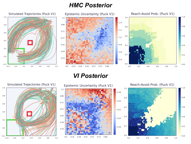
Figure 4: Top Row: Visualization of the learned system using HMC to approximately infer dynamics. Bottom Row: Visualization of the learned system using VI to approximately infer dynamics. We highlight that the VI approximation displays a 5 to 10 times reduction in epistemic uncertainty.

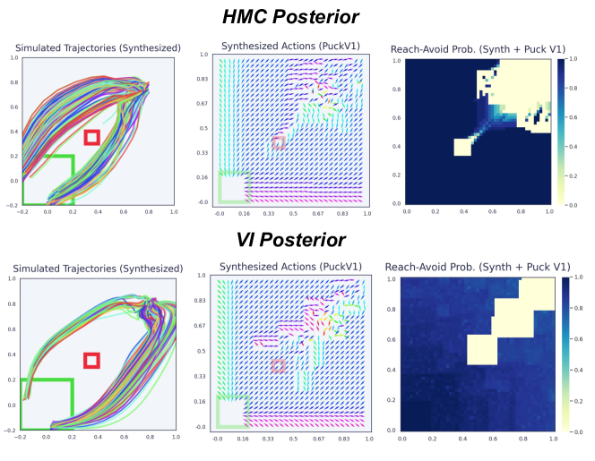
Figure 5: Top Row: Visualization of the synthesized policy and its performance based on the HMC dynamics model. Bottom Row: Visualization of the synthesized policy and its performance based on the VI dynamics model.

6.3 On the Effect of Approximate Inference

The results provided so far have been generated with BNN dynamical models learned via HMC training. However, different inference methods produce different approximations of the BNN posterior thus leading to different dynamics approximations and hence synthesized policies.

Table 2 and the plots in Figures 4 and 5 analyse the effect of approximate inference on both learned and synthesized policies, comparing results obtained by HMC with those obtained by VI training on the v1 scenario. We notice that also in the case of VI the synthesized policy significantly improves on the initial policy. Interestingly, the certification results over the learned policy for VI are higher than those obtained for HMC, but the results are comparable for the synthesized policies. In fact, it is known in the literature that VI tends to under-estimate uncertainty (Myshkov and Julier, 2016; Michelmore et al., 2020) and is more susceptible to model misspecification (Masegosa, 2020). As such, being probabilistic, the bound obtained is tighter for VI where the uncertainty is lower than that of HMC which provides a more conservative representation of the agent dynamics. For example, we see in the first two rows of Table 2 that the average lower bound achieved for the variational inference posterior is 1.88 times higher than the bounds for HMC posterior. However, our synthesis method reduces this gap between HMC and VI, while still accounting for the higher uncertainty of the former, and hence the more conservative guarantees.

While HMC approximates the posterior by relying on a Monte Carlo estimate of it, VI is a gradient-based technique, where the number of training epochs (i.e., the number of full sweeps through the dataset) is a key hyper-parameter. We thus analyse the effect of training epochs in the quality of the dynamics obtained in Figure 6, along with the effect on the synthesized policies and the certificates obtained for such policies. The left plot of the figure shows a set of predicted trajectories over a 10 time-step horizon for a varying number of training epochs, with the ground truth behaviour highlighted in red. The BNN trajectories are color-coded based on the number of epochs each dynamics model was trained for. In yellow, we see that the BNN which has only been trained for 10 epochs displays considerable error in its iterative predictions. This is reduced considerably for a model trained for 50 epochs, but the cumulative error after 10 epochs is still considerable. Finally, as expected, for models trained for 250 and 1500 epochs we empirically observe a trend toward convergence to the ground truth.

We notice that the policy and certifications directly reflect the quality of the approximation. In fact, as we increase the model fit, we see that there are significant improvements in both the intuitive behavior of the synthesized policy as well as the resulting guarantees we are able to compute.

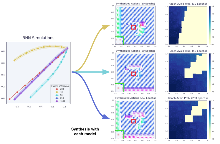
Figure 6: Analysis for number of training epochs used in performing VI training on the V1 environment. Left: sample of 10-step agent trajectories obtained with BNNs trained with VI and different number of epochs (red: ground truth trajectory). Right: synthesis and certification results for a selection of training epochs.

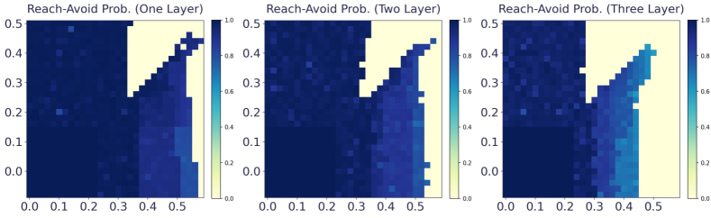
Figure 7: We vary the depth of the BNN used to learn the dynamics and observe its effects on our certified safety probabilities over the first half of the Puck-V1 state-space. From left to right we plot the lower-bound reach-avoid probabilities for a one-layer BNN dynamics model, a two-layer BNN dynamics model, and a three-layer BNN dynamics model.

6.4 Depth Experiments

In this section, we evaluate how our method performs when we vary the depth of the BNN dynamics model considered. In Figure 7, we plot the certified reach-avoid probabilities for a learned policy and a one, two, and three-layer BNN dynamics model where each layer has a width of 12 neurons. Similar architectures are found in the BNNs studied in recent related work (Lechner et al., 2021). Other than the depth of the BNN, all the other variables in the experiment are held equal (e.g., number of episodes during learning, discretization of state-space, and number of BNN samples considered for the lower bound). The learning procedure results in BNN models with roughly equivalent losses and in policies that are qualitatively similar, see A.3 for further visualizations. Given that the key factors of the system have been held equal, we notice a decrease in our certified lower bound as depth increases. Specifically, the average lower bound for the one-layer model is 0.811, for the two-layer model it is 0.763, and for the three-layer model it decreases further to 0.621. Figure 7 clearly demonstrates that as the BNN dynamics model becomes deeper, then our lower bound becomes more conservative. This finding is consistent with existing results in certification of BNNs (Wicker et al., 2020; Berrada et al., 2021) and DNNs (Gowal et al., 2018; Mirman et al., 2018). We note, however, that when the verification parameters are refined, i.e., more samples from the BNN are taken, we are able to certify the three-layer system with an average certified lower-bound of 0.867 (see A.3). These additional BNN samples increase the runtime of our certification procedure by 1.5 times.

7 Related Work

Certification of machine learning models is a rapidly growing area (Gehr et al., 2018; Katz et al., 2017; Gowal et al., 2018; Wicker et al., 2022). While most of these methods have been designed for deterministic NNs, recently safety analysis of Bayesian machine learning models has been studied both for Gaussian processes (GPs) (Grosse et al., 2017; Cardelli et al., 2019b; Blaas et al., 2020) and BNNs (Athalye et al., 2018; Cardelli et al., 2019a; Wicker et al., 2020), including methods for adversarial training (Liu et al., 2019; Wicker et al., 2021a). The above works, however, focus exclusively on the input-output behaviour of the models, that is, can only reason about static properties. Conversely, the problem we tackle in this work has additional complexity, as we aim to formally reason about iterative predictions, i.e., trajectory-level behaviour of a BNN interacting in a closed loop with a controller.

Iterative predictions have been widely studied for Gaussian processes (Girard et al., 2003) and safety guarantees have been proposed in this setting in the context of model-based RL with GPs (Jackson et al., 2020; Polymenakos et al., 2019; Berkenkamp et al., 2017, 2016). However, all these works are specific to GPs and cannot be extended to BNNs, whose posterior predictive distribution is intractable and non-Gaussian even for the more commonly employed approximate Bayesian inference methods (Neal, 2012). Recently, iterative prediction of neural network dynamic models have been studied (Wei and Liu, 2021; Adams et al., 2022) and methods to certify these models against temporal logic formulae have been derived (Adams et al., 2022). However, these works only focus on standard (i.e., non-Bayesian) neural networks with additive Gaussian noise. Closed-loop systems with known (deterministic) models and control policies modelled as BNNs are considered in (Lechner et al., 2021). In contrast with our work, Lechner et al. (2021) can only support deterministic models without noisy dynamics, only focus on the safety verification problem, and are limited to BNN posterior with unimodal weight distribution.

Various recent works consider verification or synthesis of RL schemes against reachability specifications (Sun et al., 2019; Könighofer et al., 2020; Bacci and Parker, 2020). None of these approaches, however, support both continuous state-action spaces and probabilistic models, as in this work. Continuous action spaces are supported in (Hasanbeig et al., 2019), where the authors provide RL schemes for the synthesis of policies maximising given temporal requirements, which is also extended to continuous state- and action-spaces in (Hasanbeig et al., 2020). However, the guarantees resulting from these model-free algorithms are asymptotic and thus of a different nature than those in this work. The work of Haesaert et al. (2017) integrates Bayesian inference and formal verification over control models, additionally proposing strategy synthesis approaches for active learning (Wijesuriya and Abate, 2019). In contrast to our paper these works do not support unknown noisy models learned via BNNs.

A related line of work concerns the synthesis of runtime monitors for predicting the safety of the policy’s actions and, if necessary, correct them with fail-safe actions (Alshiekh et al., 2018; Avni et al., 2019; Bouton et al., 2019; Fulton and Platzer, 2019; Phan et al., 2020). These approaches, however, do not support continuous state-action spaces or require some form of ground-truth mechanistic model for safety verification (as opposed to our data-driven BNN models).

8 Conclusions

In this paper, we considered the problem of computing the probability of time-bounded reach-avoid specifications for dynamic models described by iterative predictions of BNNs. We developed methods and algorithms to compute a lower bound of this reach-avoid probability. Additionally, relying on techniques from dynamic programming and non-convex optimization, we synthesized certified controllers that maximize probabilistic reach-avoid. In a set of experiments, we showed that our framework enables certification of strategies on non-trivial control tasks. A future research direction will be to investigate techniques to enhance the scalability of our methods so that they can be applied to state-of-the-art reinforcement learning environments. However, we emphasise that the benchmark considered in this work remains a challenging one for certification purposes, due to both the non-linearity and stochasticity of the models, and the sequential, multi-step dependency of the predictions. Thus, this paper makes an important step toward the application of BNNs in safety-critical scenarios.

Appendix A Further Experimental Details

A.1 Agent Dynamics

The puck agent is derived from a classical control problem of controlling a vehicle from an initial condition to a goal state or way point (Astrom and Murray, 2008). This scenario is more challenging than other standard benchmarks (i.e. inverted pendulum) due to both the increase state-space dimension and to the introduction of momentum which makes control more difficult. The state space of the unextended agent is a four vector containing the position in the plane as well as a vector representing the current velocity. The control signal is a two vector representing a change in the velocity (i.e. an acceleration vector). The dynamics of the puck can be given as a the following system of equations where $\eta$ determines friction, $m$ determines the mass of the puck, and $h$ determines the size of the time discretization.

$$\dot{q}=Aq+Bc$$

$$A=\begin{bmatrix}1&0&h&0\\ 0&1&0&h\\ 0&0&1-h\eta/m&0\\ 0&0&0&1-h\eta/m\\ \end{bmatrix}$$

$$B=\begin{bmatrix}0&0\\ 0&0\\ h/m&0\\ 0&h/m\\ \end{bmatrix}$$

The $n$ dimensional extension of the above dynamics is done by simply noting the structure of the matrices and generalizing them. In the upper-left of matrix $A$ we have the $2\times 2$ identity matrix which is extended to $n\times n$. Similarly, the upper-right of $A$ is extended to $h$ times the $n\times n$ identity matrix, and the lower-right is $1-h\eta/m$ times the $n\times n$ identity matrix. For each environment and including the $n$ dimensional generalizations, time resolution, $h$, is set to 0.35, the mass of the object, $m$, is fixed to $5.0$, and the friction coefficient, $\eta$, is set to 1.0.

A.2 Learning Parameters

In this section we provide the hyper-parameters used for learning an initial policy and for synthesizing NN policies. In particular, we give full parameters for the environmental interaction required to learn our policies, BNN parameters to perform approximate inference, and NN parameters for neural policy synthesis.

Episodic Parameters

In Table 3 we give the parameters for our episodic learning set up. We provide the duration (number of episodes) and the amount of data collected for each episode (number of trajectories). We highlight that as this is a model-based set up, we require many fewer simulations of the system than corresponding model-free algorithms. Each environment also has an empirically tuned maximum horizon (maximum duration for each trajectory), policy size (discretization of the state-space), and obstacle aversion, $c$, as discussed in Section 5.

Episodic Learning Parameters
	# Episodes	# Trajectories	Max Horizon	Policy Size	$c$
V1	15	20	25	$35\times 35\times 5\times 5$	0.25
V2	10	15	45	$35\times 35\times 5\times 5$	0.25
Zigzag	25	15	35	$25\times 25\times 3\times 3$	0.125

Table 3:

BNN Architectures

In Table 4, we report the HMC learning parameters for our initial set up. We give details on NN architecture size, and highlight that our hidden layer uses sigmoid activation functions while the output is equipped with a linear activation function. The burn-in perior of the HMC chain is the number of samples which are automatically not included in the posterior but help initialize the chain prior to use of the Metropolis-Rosenbluth-Hastings correction step Neal (2012). For each environmental set up we employ a leap-frog numerical integrator with 10 steps. The prior for all NN architectures is selected based on 2 times the variance perscribed by Glorot and Bengio (2010) which has shown to be an empirically well-performing prior in previous works Wicker et al. (2020, 2021a). The likelihood used to fit the BNN dynamics model is a mean squared error ($\ell_{2}$) loss function.

When using variations inference, we use 1500 epochs to fit a posterior approximated by Stochastic Weight Averaging Guassian (SWAG) which does not admit a weight-space prior. We use a learning rate of 0.025 and a decay of 0.1.

BNN Learning Parameters
	# Layers	# Neurons	Acivations	Samps.	Burn In	LR	Decay
V1	1	50	sigmoid	500	25	0.05	0.1
V2	1	50	sigmoid	500	5	0.05	0.1
Zigzag	1	50	sigmoid	250	15	0.1	0.1

Table 4:

Neural Policy Parameters

In our experiments, we employ an NN policy, $\pi_{\theta}$, comprised of a single hidden layer with 36 neurons. This is first trained to mimic actions that are sampled randomly at uniform. This training is done with SGD and is done for 15000 sampled states and actions. The NN policy is trained with 100 epochs of stochastic gradient descent with learning rate 0.00075 every time it is trained. This occurs after a BNN has been fit and used to update the actions according to loss presented in Section 5 save for no adversarial noise is taken into consideration. When we do perform synthesis, all of the same parameters are used: 15000 actions are considered and updated in parallel by SGD w.r.t. the adversarial loss defined in Section 5.

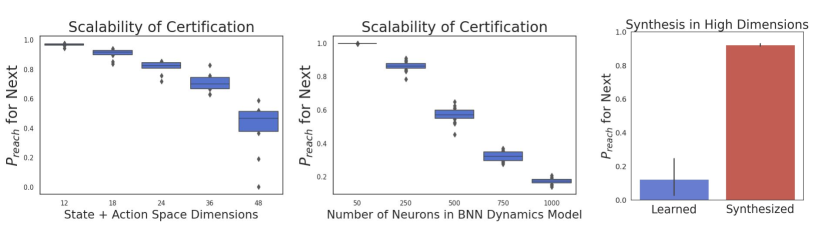
Figure 8: Left: Certified lower bound for forward invariance with respect to an increasing number of state-space dimensions. Center: Certified lower bound as a function of the width of the BNN Right: Comparison between synthesised policy and learned policy on the 12-dimensional puck problem.

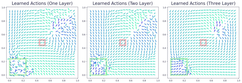
Figure 9: We plot the learned policies corresponding to each of the dynamical systems whose certification is visualized in Figure 7. The left plot is the policy learned along with a one-layer BNN, the center plot is the policy learned along with a two-layer BNN, and the right plot is the policy learned along with a three-layer BNN.

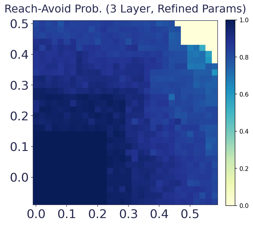
Figure 10: Lower-bound reach-avoid probabilities for the three layer BNN after refining the certification parameters from the procedure in Figure 7.

A.3 Further Scalability Experiments

In this section we provide further analysis and discussion of experiments on BNN depth in our framework and provide further experiments exploring how our method scales with state-space dimensions.

A.3.1 Further Detail on BNN Depth Experiments

In Figure 9 we plot the policies that correspond to each of the BNNs learned for our depth experiments discussed in Section 6.4 and visualized in Figure 7. We highlight that each of the policies are qualitatively very similar, though they may have slight quantitative differences. In Figure 10 we plot the result of the more computationally expensive certification on the three-layer BNN. Though our method struggles to get strong certification for the system with a three-layer BNN in Figure 7, by tuning the certification parameters we are able to get a much tighter lower-bound (average lower-bound safety probability $0.621\rightarrow 0.867$). We notice that many of the previously uncertified (i.e., lower-bound probability 0.0) states have lower-bounds above 0.6 when more BNN samples are used in the certification procedure.

A.3.2 Scaling with State-Space Dimensionality

In this section, we evaluate how our method performs while varying the dimensionality of the environment and the size of the BNN architecture. In particular we perform the analyses using an $n$-dimensional generalizations of the v1 layout - described by $3n$ continuous values, $n$ dimensions for position, velocity, and action spaces, respectively. For such high-dimensional state space, full discretisation of the state space becomes infeasible. In order to overcome this, we consider a forward-invariance variant of the reach-avoid property from our previous experiments, where the agent goal is iteratively moved at each step in order to guide it to the global goal. In other words, here we consider one-step reachability ($N=1$), which allows us to significantly reduce the set of discretised states to consider (by restricting to neighbour states that can be reached in one step only).

The results for these analyses are given in Figure 8. The left plot of the figure, shows how even for 48 dimensions we are still able to obtain non-vacous bounds at $0.5$, but as expected, the quality of the bound decreases quickly with the size of the state space and actions. The centre plot depicts the certified bounds obtained for an increasing number of BNN hidden units, up until $1000$ for the 12-dimensional v1 scenario. Finally, the right plot of Figure 8 shows that our synthesis algorithm strongly improves on the initially learned policy, even in higher-dimensional settings. We accomplish this improvement by following the neural policy synthesis method presented in Section 5 where the worst-case $\epsilon$ for tuning our actions is set to 0.025.

This analysis of the forward invariance property allows us to understand how our algorithm, particularly the evaluation of the $R$ function, scales to larger NNs and state spaces. However, for state-space dimensions that are greater than the ones analyzed in the prior section of this paper, certification of the entire state-space is computationally infeasible due to the exponential nature of the discretization involved.

Appendix B Proofs

Proof of Proposition 1 In what follows, we omit $\pi$ (which is given and held constant) from the probabilities for a more compact notation. The proof is by induction. The base case is $k=N$, for which we have

$$V_{N}^{\pi}(x)=\mathbf{1}_{\mathrm{G}}(x)=P_{reach}(\mathrm{G},\mathrm{S},x,[N,N]),$$

which holds trivially. Under the assumption that, for any given $k\in[0,N-1]$, it holds that

$$V_{k+1}^{\pi}(x)=P_{reach}(\mathrm{G},\mathrm{S},x,[k+1,N]),$$ (15)

we show the induction step for time step $k$. In particular,

$$P_{reach}(\mathrm{G},\mathrm{S},x,[k,N]|\pi)=$$

$$Pr(\mathbf{x}_{k}\in\mathrm{G}|\mathbf{x}_{k}=x)+\sum_{j=k+1}^{N}Pr(\mathbf{x}_{j}\in\mathrm{G}\wedge\forall j^{\prime}\in[k,j),\mathbf{x}_{j^{\prime}}\in\mathrm{S}|\mathbf{x}_{k}=x)=$$

$$\mathbf{1}_{\mathrm{G}}(x)+\mathbf{1}_{\mathrm{S}}(x)\sum_{j=k+1}^{N}Pr(\mathbf{x}_{j}\in\mathrm{G}\wedge\forall j^{\prime}\in[k,j),\mathbf{x}_{j^{\prime}}\in\mathrm{S}|\mathbf{x}_{k}=x)$$

Now in order to conclude the proof we want to show that

$$\sum_{j=k+1}^{N}Pr(\mathbf{x}_{j}\in\mathrm{G}\wedge\forall j^{\prime}\in[k,j)+1,\mathbf{x}_{j^{\prime}}\in\mathrm{S}| \mathbf{x}_{k}=x)=$$

$$\int V_{k+1}^{\pi}(\bar{x})p(\bar{x}\mid(x,\pi_{k}(x)),\mathcal{D})d\bar{x}.$$

This can be done as follow

$$\sum_{j=k+1}^{N}Pr(\mathbf{x}_{j}\in\mathrm{G}\wedge\forall j^{\prime}\in[k+1,j),\mathbf{x}_{j^{\prime}}\in\mathrm{S}|\mathbf{x}_{k}=x)=$$

$$Pr(\mathbf{x}_{k+1}\in\mathrm{G}|\mathbf{x}_{k}=x)+$$

$$\quad\sum_{j=k+2}^{N}Pr(\mathbf{x}_{j}\in\mathrm{G}\wedge\forall j^{\prime}\in[k+1,j),\mathbf{x}_{j^{\prime}}\in\mathrm{S}|\mathbf{x}_{k}=x)=$$

$$\int_{\mathrm{G}}p(\bar{x}\mid(x,\pi_{k}(x)),\mathcal{D})d\bar{x}+$$

$$\quad\sum_{j=k+2}^{N}\int_{\mathrm{S}}Pr(\mathbf{x}_{j}\in\mathrm{G}\wedge\forall j^{\prime}\in[k+2,j),\mathbf{x}_{j^{\prime}}\in\mathrm{S}\wedge\mathbf{x}_{k+1}=\bar{x}|\mathbf{x}_{k}=x)d\bar{x}=$$

$$\int_{\mathrm{G}}p(\bar{x}\mid(x,\pi_{k}(x)),\mathcal{D})d\bar{x}+$$

$$\quad\sum_{j=k+2}^{N}\int_{\mathrm{S}}Pr(\mathbf{x}_{j}\in\mathrm{G}\wedge\forall j^{\prime}\in[k+2,j),\mathbf{x}_{j^{\prime}}\in\mathrm{S}|\mathbf{x}_{k+1}=\bar{x})p(\bar{x}\mid(x,\pi_{k}(x)),\mathcal{D})d{\bar{x}}=$$

$$\int\big{(}\mathbf{1}_{\mathrm{G}}(\bar{x})+$$

$$\quad\mathbf{1}_{\mathrm{S}}(\bar{x})\sum_{j=k+2}^{N}Pr(\mathbf{x}_{j}\in\mathrm{G}\wedge\forall j^{\prime}\in[k+2,j),\mathbf{x}_{j^{\prime}}\in\mathrm{S}|\mathbf{x}_{k+1}=\bar{x})\big{)}p(\bar{x}\mid(x,\pi_{k}(x)),\mathcal{D})d{\bar{x}}=$$

$$\int V_{k+1}^{\pi}(\bar{x})p(\bar{x}\mid(x,\pi_{k}(x)),\mathcal{D})d{\bar{x}}$$

where the third step holds by application of Bayes rule over multiple events.

Proof of Theorem 1 The proof is by induction. The base case is $k=N$, for which we have

$$\inf_{x\in q}V_{N}^{\pi}(x)=\inf_{x\in q}\mathbf{1}_{\mathrm{G}}(x)=\mathbf{1}_{\mathrm{G}}(q)=K_{N}^{\pi}(q).$$

Next, under the assumption that for any $k\in\{0,N-1\}$ it holds that

$$\inf_{x\in q}V_{k+1}^{\pi}(x)\geq K_{k+1}^{\pi}(q),$$

we can work on the induction step: in order to derive it, it is enough to show that for any $\epsilon>0$

$$\int V_{k+1}^{\pi}(\bar{x})p(\bar{x}\mid(x,\pi_{k}(x)),\mathcal{D})d\bar{x}\geq$$

$$\quad F([-\epsilon,\epsilon]|\sigma^{2})^{n}\sum_{i=1}^{n_{p}}\int_{H^{q,\pi}_{k,i}}v_{i-1}p_{\mathbf{w}}(w|\mathcal{D})dw,$$

where $F([-\epsilon,\epsilon]|\sigma^{2})=\text{erf}(\frac{\epsilon}{\sqrt{2\sigma^{2}}})$ is the cumulative function distribution for a normal random variable with zero mean and variance $\sigma^{2}$ being within $[-\epsilon,\epsilon].$ This can be argued by rewriting the first term in parameter space (recall that the stochastic kernel $T$ is induced by $p_{\mathbf{w}}(w|\mathcal{D})$) and providing a lower bound, as follows:

$$\int V_{k+1}^{\pi}(\bar{x})p(\bar{x}\mid(x,\pi_{k}(x)),\mathcal{D})d\bar{x}=$$

(By definition of predictive distribution)

$$\int\big{(}\int V_{k+1}^{\pi}(\bar{x})p(\bar{x}|(x,u),w)d\bar{x}\big{)}p_{\mathbf{w}}(w|\mathcal{D})dw\geq$$

(By $$V_{k+1}^{k}$$ being non negative everywhere and by the Gaussian likelihood)

$$\int\big{(}\int_{f^{w}(x,\pi(x,k))+\epsilon}^{f^{w}(x,\pi(x,k)-\epsilon}V_{k+1}^{\pi}(\bar{x})\mathcal{N}(\bar{x}|f^{w}(x,\pi(x,k)),\sigma^{2}\cdot I)d\bar{x}\big{)}p_{\mathbf{w}}(w|\mathcal{D})dw\geq$$

(By standard inequalities of integrals)

$$\int\inf_{\bar{\gamma}\in[-\epsilon,\epsilon]}V_{k+1}^{\pi}(f^{w}(x,\pi(x,k)+\bar{\gamma})\big{(}\int_{[-\epsilon,\epsilon]^{n}}\mathcal{N}(\gamma|0,\sigma^{2})d\gamma\big{)}^{n}p_{\mathbf{w}}(w|\mathcal{D})dw\geq$$

(By the assumptions that for $$i\neq j H^{q,\pi}_{k,i} H^{q,\pi}_{k,j}$$ and are non-overlapping)

$$\big{(}\int_{[-\epsilon,\epsilon]}\mathcal{N}(\gamma|0,\sigma^{2})d\gamma\big{)}^{n}\sum_{i=1}^{n_{p}}\int_{H^{q,\pi,\epsilon}_{k,i}}\inf_{\bar{\gamma}\in[-\epsilon,\epsilon]}V_{k+1}^{\pi}(f^{w}(x,\pi(x,k)+\bar{\gamma})p_{\mathbf{w}}(w|\mathcal{D})dw,$$

(By the fact that $$v_{i}\leq\inf_{x\in q}V_{k+1}^{\pi}(f^{w}(x,\pi(x,k)+\bar{\gamma})$$ )

$$\big{(}\int_{[-\epsilon,\epsilon]}\mathcal{N}(\gamma|0,\sigma^{2})d\gamma\big{)}^{n}\sum_{i=1}^{n_{p}}v_{i}\int_{H^{q,\pi,\epsilon}_{k,i}}p_{\mathbf{w}}(w|\mathcal{D})dw,$$

where the last step concludes the proof because, by the induction hypothesis, we know that for $q^{\prime}\subseteq\mathbb{R}^{n}$

$$\inf_{\bar{x}\in q^{\prime}}V_{k+1}^{\pi}(\bar{x})\geq K_{k+1}^{\pi}(q^{\prime})$$

and by the construction of sets $H^{q,\pi}_{k,i}$ for each of its weights $K_{k+1}^{\pi}(f^{w}(\bar{x},\pi(x,k))$ is lower bounded by $v_{i-1}$.

References

- Abate et al. (2008) Alessandro Abate, Maria Prandini, John Lygeros, and Shankar Sastry. Probabilistic reachability and safety for controlled discrete time stochastic hybrid systems. Automatica, 44(11):2724–2734, 2008.
- Adams et al. (2022) Steven Adams, Morteza Lahijanian, and Luca Laurenti. Formal control synthesis for stochastic neural network dynamic models. arXiv preprint arXiv:2203.05903, 2022.
- Alshiekh et al. (2018) Mohammed Alshiekh, Roderick Bloem, Rüdiger Ehlers, Bettina Könighofer, Scott Niekum, and Ufuk Topcu. Safe reinforcement learning via shielding. In Proceedings of the AAAI Conference on Artificial Intelligence, volume 32, 2018.
- Astrom and Murray (2008) Karl J. Astrom and Richard M. Murray. Feedback Systems: An Introduction for Scientists and Engineers. Princeton University Press, Princeton, NJ, USA, 2008.
- Athalye et al. (2018) Anish Athalye, Nicholas Carlini, and David Wagner. Obfuscated gradients give a false sense of security: Circumventing defenses to adversarial examples. In International Conference on Machine Learning, pages 274–283. PMLR, 2018.
- Avni et al. (2019) Guy Avni, Roderick Bloem, Krishnendu Chatterjee, Thomas A Henzinger, Bettina Könighofer, and Stefan Pranger. Run-time optimization for learned controllers through quantitative games. In International Conference on Computer Aided Verification, pages 630–649. Springer, 2019.
- Bacci and Parker (2020) Edoardo Bacci and David Parker. Probabilistic guarantees for safe deep reinforcement learning. In International Conference on Formal Modeling and Analysis of Timed Systems, pages 231–248. Springer, 2020.
- Berkenkamp et al. (2016) Felix Berkenkamp, Angela P. Schoellig, and Andreas Krause. Safe controller optimization for quadrotors with Gaussian processes. In Proc. of the IEEE International Conference on Robotics and Automation (ICRA), pages 493–496, 2016.
- Berkenkamp et al. (2017) Felix Berkenkamp, Matteo Turchetta, Angela P Schoellig, and Andreas Krause. Safe model-based reinforcement learning with stability guarantees. In NIPS, 2017.
- Berrada et al. (2021) Leonard Berrada, Sumanth Dathathri, Krishnamurthy Dvijotham, Robert Stanforth, Rudy R Bunel, Jonathan Uesato, Sven Gowal, and M Pawan Kumar. Make sure you’re unsure: A framework for verifying probabilistic specifications. Advances in Neural Information Processing Systems, 34:11136–11147, 2021.
- Bertsekas and Shreve (2004) Dimitir P Bertsekas and Steven Shreve. Stochastic optimal control: the discrete-time case. Athena Scientific, 2004.
- Blaas et al. (2020) Arno Blaas, Andrea Patane, Luca Laurenti, Luca Cardelli, Marta Kwiatkowska, and Stephen Roberts. Adversarial robustness guarantees for classification with Gaussian processes. In International Conference on Artificial Intelligence and Statistics, pages 3372–3382. PMLR, 2020.
- Blundell et al. (2015) Charles Blundell, Julien Cornebise, Koray Kavukcuoglu, and Daan Wierstra. Weight uncertainty in neural network. In International Conference on Machine Learning, pages 1613–1622. PMLR, 2015.
- Bouton et al. (2019) Maxime Bouton, Jesper Karlsson, Alireza Nakhaei, Kikuo Fujimura, Mykel J Kochenderfer, and Jana Tumova. Reinforcement learning with probabilistic guarantees for autonomous driving. arXiv preprint arXiv:1904.07189, 2019.
- Carbone et al. (2020) Ginevra Carbone, Matthew Wicker, Luca Laurenti, Andrea Patane', Luca Bortolussi, and Guido Sanguinetti. Robustness of bayesian neural networks to gradient-based attacks. In H. Larochelle, M. Ranzato, R. Hadsell, M. F. Balcan, and H. Lin, editors, Advances in Neural Information Processing Systems, volume 33, pages 15602–15613. Curran Associates, Inc., 2020.
- Cardelli et al. (2019a) Luca Cardelli, Marta Kwiatkowska, Luca Laurenti, Nicola Paoletti, Andrea Patane, and Matthew Wicker. Statistical guarantees for the robustness of bayesian neural networks. In Proceedings of the Twenty-Eighth International Joint Conference on Artificial Intelligence, IJCAI-19, pages 5693–5700. International Joint Conferences on Artificial Intelligence Organization, 7 2019a. doi: 10.24963/ijcai.2019/789. URL https://doi.org/10.24963/ijcai.2019/789.
- Cardelli et al. (2019b) Luca Cardelli, Marta Kwiatkowska, Luca Laurenti, and Andrea Patane. Robustness guarantees for Bayesian inference with Gaussian processes. In Proceedings of the AAAI Conference on Artificial Intelligence, volume 33, pages 7759–7768, 2019b.
- Cauchi et al. (2019) Nathalie Cauchi, Luca Laurenti, Morteza Lahijanian, Alessandro Abate, Marta Kwiatkowska, and Luca Cardelli. Efficiency through uncertainty: Scalable formal synthesis for stochastic hybrid systems. In Proceedings of the 22nd ACM International Conference on Hybrid Systems: Computation and Control, pages 240–251, 2019.
- Deisenroth and Rasmussen (2011) Marc Peter Deisenroth and Carl Edward Rasmussen. PILCO: A model-based and data-efficient approach to policy search. In In Proceedings of the International Conference on Machine Learning, 2011.
- Depeweg et al. (2017) S Depeweg, JM Hernández-Lobato, F Doshi-Velez, and S Udluft. Learning and policy search in stochastic dynamical systems with bayesian neural networks. In 5th International Conference on Learning Representations, ICLR 2017-Conference Track Proceedings, 2017.
- Fubini (1907) Guido Fubini. Sugli integrali multipli. Rend. Acc. Naz. Lincei, 16:608–614, 1907.
- Fulton and Platzer (2019) Nathan Fulton and André Platzer. Verifiably safe off-model reinforcement learning. In International Conference on Tools and Algorithms for the Construction and Analysis of Systems, pages 413–430. Springer, 2019.
- Gal et al. (2016a) Yarin Gal, Rowan McAllister, and Carl Edward Rasmussen. Improving PILCO with Bayesian neural network dynamics models. In International Conference in Machine Learning (ICML), 2016a.
- Gal et al. (2016b) Yarin Gal, Rowan Thomas McAllister, and Carl Edward Rasmussen. Improving PILCO with Bayesian neural network dynamics models. In Data-Efficient Machine Learning workshop, volume 951, page 2016, 2016b.
- Gehr et al. (2018) Timon Gehr, Matthew Mirman, Dana Drachsler-Cohen, Petar Tsankov, Swarat Chaudhuri, and Martin Vechev. Ai2: Safety and robustness certification of neural networks with abstract interpretation. In 2018 IEEE S&P, pages 3–18. IEEE, 2018.
- Girard et al. (2003) Agathe Girard, Carl Edward Rasmussen, Joaquin Quinonero Candela, and Roderick Murray-Smith. Gaussian process priors with uncertain inputs application to multiple-step ahead time series forecasting. In Advances in neural information processing systems, pages 545–552, 2003.
- Glorot and Bengio (2010) Xavier Glorot and Yoshua Bengio. Understanding the difficulty of training deep feedforward neural networks. In Proceedings of the thirteenth international conference on artificial intelligence and statistics, pages 249–256. JMLR Workshop and Conference Proceedings, 2010.
- Goodfellow et al. (2016) Ian Goodfellow, Yoshua Bengio, and Aaron Courville. Deep learning. MIT press, 2016.
- Gowal et al. (2018) Sven Gowal, Krishnamurthy Dvijotham, Robert Stanforth, Rudy Bunel, Chongli Qin, Jonathan Uesato, Relja Arandjelovic, Timothy Mann, and Pushmeet Kohli. On the effectiveness of interval bound propagation for training verifiably robust models. Neural Information Processing Systems (NeurIPS), 2018.
- Grosse et al. (2017) Kathrin Grosse, David Pfaff, Michael Thomas Smith, and Michael Backes. How wrong am i?-studying adversarial examples and their impact on uncertainty in gaussian process machine learning models. arXiv preprint arXiv:1711.06598, 2017.
- Haesaert et al. (2017) S. Haesaert, P.M.J. V.d. Hof, and A. Abate. Data-driven and model-based verification via Bayesian identification and reachability analysis. Automatica, 79(5):115–126, 2017.
- Hasanbeig et al. (2020) M. Hasanbeig, D. Kroening, and A. Abate. Deep reinforcement learning with temporal logics. In Proceedings of FORMATS, LNCS 12288, pages 1–22, 2020.
- Hasanbeig et al. (2019) Mohammadhosein Hasanbeig, Alessandro Abate, and Daniel Kroening. Certified reinforcement learning with logic guidance. arXiv preprint arXiv:1902.00778, 2019.
- Huang and Rosendo (2020) Jingyi Huang and Andre Rosendo. Deep vs. deep bayesian: Reinforcement learning on a multi-robot competitive experiment. arXiv preprint arXiv:2007.10675, 2020.
- Izmailov et al. (2021) Pavel Izmailov, Sharad Vikram, Matthew D Hoffman, and Andrew Gordon Gordon Wilson. What are bayesian neural network posteriors really like? In International conference on machine learning, pages 4629–4640. PMLR, 2021.
- Jackson et al. (2020) John Jackson, Luca Laurenti, Eric Frew, and Morteza Lahijanian. Safety verification of unknown dynamical systems via gaussian process regression. In 2020 59th IEEE Conference on Decision and Control (CDC), pages 860–866. IEEE, 2020.
- Katz et al. (2017) Guy Katz, Clark Barrett, David L Dill, Kyle Julian, and Mykel J Kochenderfer. Reluplex: An efficient SMT solver for verifying deep neural networks. In International Conference on Computer Aided Verification, pages 97–117. Springer, 2017.
- Khan and Rue (2021) Mohammad Emtiyaz Khan and Håvard Rue. The bayesian learning rule. arXiv preprint arXiv:2107.04562, 2021.
- Könighofer et al. (2020) Bettina Könighofer, Roderick Bloem, Sebastian Junges, Nils Jansen, and Alex Serban. Safe reinforcement learning using probabilistic shields. In International Conference on Concurrency Theory: 31st CONCUR 2020: Vienna, Austria (Virtual Conference). Schloss Dagstuhl-Leibniz-Zentrum fur Informatik GmbH, Dagstuhl Publishing, 2020.
- Kwiatkowska et al. (2007) Marta Kwiatkowska, Gethin Norman, and David Parker. Stochastic model checking. In International School on Formal Methods for the Design of Computer, Communication and Software Systems, pages 220–270. Springer, 2007.
- Lechner et al. (2021) Mathias Lechner, Đorđe Žikelić, Krishnendu Chatterjee, and Thomas Henzinger. Infinite time horizon safety of bayesian neural networks. Advances in Neural Information Processing Systems, 34, 2021.
- Liang (2005) Faming Liang. Bayesian neural networks for nonlinear time series forecasting. Statistics and computing, 15(1):13–29, 2005.
- Liu et al. (2019) Xuanqing Liu, Yao Li, Chongruo Wu, and Cho-Jui Hsieh. Adv-bnn: Improved adversarial defense through robust Bayesian neural network. 7th International Conference on Learning Representations, ICLR 2019-Conference Track Proceedings, 2019.
- Madry et al. (2017) Aleksander Madry, Aleksandar Makelov, Ludwig Schmidt, Dimitris Tsipras, and Adrian Vladu. Towards deep learning models resistant to adversarial attacks. arXiv preprint arXiv:1706.06083, 2017.
- Masegosa (2020) Andres Masegosa. Learning under model misspecification: Applications to variational and ensemble methods. Advances in Neural Information Processing Systems, 33:5479–5491, 2020.
- McAllister and Rasmussen (2017) Rowan McAllister and Carl Edward Rasmussen. Data-efficient reinforcement learning in continuous state-action gaussian-pomdps. In I. Guyon, U. V. Luxburg, S. Bengio, H. Wallach, R. Fergus, S. Vishwanathan, and R. Garnett, editors, Advances in Neural Information Processing Systems, volume 30. Curran Associates, Inc., 2017.
- Michelmore et al. (2020) Rhiannon Michelmore, Matthew Wicker, Luca Laurenti, Luca Cardelli, Yarin Gal, and Marta Kwiatkowska. Uncertainty quantification with statistical guarantees in end-to-end autonomous driving control. In 2020 IEEE International Conference on Robotics and Automation (ICRA), pages 7344–7350. IEEE, 2020.
- Mirman et al. (2018) Matthew Mirman, Timon Gehr, and Martin Vechev. Differentiable abstract interpretation for provably robust neural networks. In International Conference on Machine Learning, pages 3578–3586. PMLR, 2018.
- Murphy (2012) Kevin P Murphy. Machine learning: a probabilistic perspective. MIT press, 2012.
- Myshkov and Julier (2016) Pavel Myshkov and Simon Julier. Posterior distribution analysis for bayesian inference in neural networks. In Workshop on Bayesian Deep Learning, NIPS, 2016.
- Neal (2012) Radford M Neal. Bayesian learning for neural networks, volume 118. Springer Science & Business Media, 2012.
- Neal et al. (2011) Radford M Neal et al. Mcmc using hamiltonian dynamics. Handbook of markov chain monte carlo, 2(11):2, 2011.
- Phan et al. (2020) Dung T Phan, Radu Grosu, Nils Jansen, Nicola Paoletti, Scott A Smolka, and Scott D Stoller. Neural simplex architecture. In NASA Formal Methods Symposium, pages 97–114. Springer, 2020.
- Polymenakos et al. (2019) Kyriakos Polymenakos, Alessandro Abate, and Stephen Roberts. Safe policy search using Gaussian process models. In Proceedings of the 18th International Conference on Autonomous Agents and Multi Agent Systems, pages 1565–1573. IFAAMS, 2019.
- Polymenakos et al. (2020) Kyriakos Polymenakos, Luca Laurenti, Andrea Patane, Jan-Peter Calliess, Luca Cardelli, Marta Kwiatkowska, Alessandro Abate, and Stephen Roberts. Safety guarantees for iterative predictions with Gaussian processes. In 2020 59th IEEE Conference on Decision and Control (CDC), pages 3187–3193. IEEE, 2020.
- Schrittwieser et al. (2019) Julian Schrittwieser, Ioannis Antonoglou, Thomas Hubert, Karen Simonyan, Laurent Sifre, Simon Schmitt, Arthur Guez, Edward Lockhart, Demis Hassabis, Thore Graepel, et al. Mastering atari, go, chess and shogi by planning with a learned model. corr abs/1911.08265 (2019). arXiv preprint arXiv:1911.08265, 2019.
- Soudjani and Abate (2013) S. Esmaeil Zadeh Soudjani and A. Abate. Probabilistic reach-avoid computation for partially-degenerate stochastic processes. IEEE Transactions on Automatic Control, 58(12):528–534, 2013.
- Sun et al. (2019) Xiaowu Sun, Haitham Khedr, and Yasser Shoukry. Formal verification of neural network controlled autonomous systems. In Proceedings of the 22nd ACM International Conference on Hybrid Systems: Computation and Control, pages 147–156, 2019.
- Sutton and Barto (1998) Richard S Sutton and Andrew G Barto. Reinforcement learning: An introduction, 1998.
- Vinogradska et al. (2016) Julia Vinogradska, Bastian Bischoff, Duy Nguyen-Tuong, Anne Romer, Henner Schmidt, and Jan Peters. Stability of controllers for gaussian process forward models. In International Conference on Machine Learning, pages 545–554. PMLR, 2016.
- Wei and Liu (2021) Tianhao Wei and Changliu Liu. Safe control with neural network dynamic models. arXiv preprint arXiv:2110.01110, 2021.
- Wicker (2021) Matthew Wicker. Adversarial robustness of Bayesian neural networks. PhD thesis, University of Oxford, 2021.
- Wicker et al. (2020) Matthew Wicker, Luca Laurenti, Andrea Patane, and Marta Kwiatkowska. Probabilistic safety for bayesian neural networks. In Jonas Peters and David Sontag, editors, Proceedings of the 36th Conference on Uncertainty in Artificial Intelligence (UAI), volume 124 of Proceedings of Machine Learning Research, pages 1198–1207. PMLR, 03–06 Aug 2020.
- Wicker et al. (2021a) Matthew Wicker, Luca Laurenti, Andrea Patane, Zhuotong Chen, Zheng Zhang, and Marta Kwiatkowska. Bayesian inference with certifiable adversarial robustness. In Arindam Banerjee and Kenji Fukumizu, editors, Proceedings of The 24th International Conference on Artificial Intelligence and Statistics, volume 130 of Proceedings of Machine Learning Research, pages 2431–2439. PMLR, 13–15 Apr 2021a.
- Wicker et al. (2021b) Matthew Wicker, Luca Laurenti, Andrea Patane, Nicola Paoletti, Alessandro Abate, and Marta Kwiatkowska. Certification of iterative predictions in bayesian neural networks. In Uncertainty in Artificial Intelligence, pages 1713–1723. PMLR, 2021b.
- Wicker et al. (2022) Matthew Robert Wicker, Juyeon Heo, Luca Costabello, and Adrian Weller. Robust explanation constraints for neural networks. In The Eleventh International Conference on Learning Representations, 2022.
- Wijesuriya and Abate (2019) V. Wijesuriya and A. Abate. Bayes-adaptive planning for data-efficient verification of uncertain Markov decision processes. In Proceedings of QEST, LNCS 11785, pages 91–108, 2019.