Homotopy-Aware Multi-Agent Path Planning in Plane

Abstract

We propose an efficient framework using the Dehornoy order for homotopy-aware multi-agent path planning in the plane. We developed a method to generate homotopically distinct solutions of multi-agent path planning problem in the plane by combining our framework with revised prioritized planning and proved its completeness under specific assumptions. Experimentally, we demonstrated that the runtime of our method grows approximately quintically with the number of agents. We also confirmed the usefulness of homotopy-awareness by showing experimentally that generation of homotopically distinct solutions by our method contributes to planning low-cost trajectories for a swarm of agents.

1 Introduction

In robot planning and navigation, considering topological features of paths is crucial in various aspects. It becomes particularly significant when seeking globally optimal trajectories. While a conventional strategy is to plan an initial path on the simple graph (e.g., grid) and optimize it to minimize cost, it may lead to local optima since optimization does not alter topological characteristics. Since which path is optimized to a globally optimal solution cannot be known beforehand, it was proposed to generate several topologically district paths [45, 64]. Topological awareness in planning also finds relevance in tasks such as cables manipulation [13, 41], human-robot interaction [31, 78], and high-level planning with dynamic obstacles [16].

Homotopy is a straightforward topological feature of paths, but difficult to calculate due to its non-abelian nature. Bhattacharya and Ghrist [9] proposed an approach on the basis of the concept called homotopy-augmented graph for general homotopy-aware path planning. Homotopy-aware path planning using a roadmap is reduced to pathfinding on homotopy-augmented graph constructed from the roadmap. To search on the homotopy-augmented graph, we have to manage elements of the homotopy group of the searched space. Elements are represented by strings of generators, called words. However, different words can represent the same element of the group and determining the identity of such representations, termed the word problem, is not generally solvable [58]. Consequently, homotopy-aware path planning remains a generally difficult task.

On the other hand, multi-agent path planning, which plans paths for multiple agents so that they do not collide each other, has a variety of application [68, 22, 50]. In multi-agent scenario on the plane, topological features are important even in absence of obstacle since other agents are obstacles for agents [56]. For example, when two agents pass each other, the topological characteristics of the solution differ depending on whether they avoid each other counterclockwise or clockwise as shown in Fig. 1. Nevertheless, studies on topology-aware planning for multi-agent scenarios, even in obstacle-free environments, are limited.

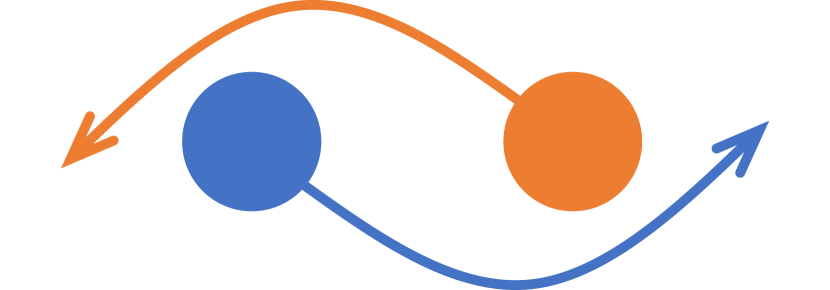
(a) Counterclockwise

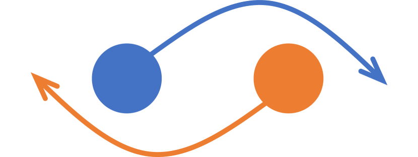
(b) Clockwise

Figure 1: Two ways for two agents to pass each other

By combining the aforementioned concepts with research in the area of pure mathematics, we obtained an efficient framework for homotopy-aware multi-agent path planning on the plane, which is the first valid solution of this problem to our knowledge. There are two key ideas. First, while solving a classical (labeled) multi-agent path planning problem, we calculate homotopy class as solutions of an unlabeled multi-agent path planning problem, in which, as long as each goal is reached by only one agent, it is permissible for any agent to proceed to any goal. [1]. Since homotopy classes inherently contain information about agent-goal correspondences, this idea does not give rise to any confusion. The homotopy group for unlabeled multi-agent path planning is the braid group [30]. The second idea is to use the Dehornoy order, a linear order on the braid groups [18], for which there are efficient comparison algorithms [20]. Thanks to the linearity of the Dehornoy order, we can not only solve the word problem but also efficiently maintain the homotopy-augmented graph by using a data structure such as self-balancing binary search trees [43].

By combining this framework with the revised prioritized planning [17], we obtained a method to generate homotopically distinct solutions of multi-agent path planning in the plane. We also proved that our method can generate solutions belonging to all homotopy classes under certain assumptions.

We experimentally demonstrated that the runtime of our method grows approximately quintically with respect to the number of agents. In addition, to confirm the usefulness of homotopy-awareness in this situation, we experimentally show that optimizing homotopically distinct solutions generated by our method leads to finding low-cost trajectories.

In summary, the contributions of this paper are that it proposed the first sound algorithm for solving homotopy-aware multi-agent path planning and that it experimentally showed that solving this problem contributes to trajectory optimization.

2 Related Work

2.1 Multi-Agent Path Planning

Multi-agent pathfinding, a field of study focusing on planning for multiple agents in discrete graphs, has been a subject of extensive research, particularly in grid-based environments [70]. One of the approaches for this problem is prioritized planning [25, 68], which is non-optimal, incomplete yet scalable. Čáp et al. [17] proposed a revised version of prioritized planning and proved its completeness under certain assumptions. Among the major optimal approaches for multi-agent pathfinding are increasing-cost tree search [66], conflict-based search [67], and some reduction-based methods [72, 6]. Surveys of solutions have been conducted by Stern [69] and Lejeune et al. [48].

For multi-agent path planning in continuous environments, a typical strategy involves a three-step process: roadmap generation, discrete pathfinding, and, if necessary, continuous smoothing of trajectories. For instance, Hönig et al. [38] presented such an approach to apply to quadrotor swarm navigation. Several roadmap-generation methods tailored for multi-agent scenarios have been proposed [36, 3, 59]. A number of multi-agent pathfinding algorithms have been adapted to handle continuous time scenarios [76, 75, 2, 71].

2.2 Topology-Aware Path Planning

For homotopy-aware single-agent path planning in the plane with polygonal obstacles, there exist methods using polygon partition [60, 51] with analysis of time complexity [37, 23, 7]. For scenarios involving possibly non-polygonal obstacles, several approaches have been explored [39, 37, 78, 65]. Grigoriev and Slissenko [32, 33] proposed a method of constructing words by detecting traversing cuts, which are also called rays [73]. Along this idea, the notion of homotopy-augmented graph (h-augmented graph), was proposed and applied to the navigation of a mobile robot with a cable [13, 41]. This approach was generalized by Bhattacharya and Ghrist [9] to various situations including multi-agent path planning in the plane. However, their algorithm is incomplete. While they attempted to solve the word problem by using Dehn’s algorithm [52], they acknowledged that this algorithm may not always yield accurate results for their presentation.

Homology serves as a coarser classification compared with homotopy, whereby two paths belonging to the same homotopy class are also in the same homology class, but the reverse is not always true. While homology is not well-suited for detailed path analysis like homotopy, it possesses the advantage of being computationally easier due to its abelian nature. Algorithms have been developed for homology-aware path planning in two, three, or higher dimensional Euclidean spaces with obstacles [8, 10, 11, 12]. In the planar scenario, homology can be determined by winding numbers [74] and this knowledge has been applied to enable homology-aware planning for mobile robot navigation [45]. Winding number is also used for navigation when other agents are present [57].

2.3 Braids and their Applications to Robotics

The braid group was introduced by Artin [4, 5]. There are several algorithms for solving the word problem of the braid groups [28, 24, 15, 34, 27]. The Dehornoy order was introduced by Dehornoy [18], who also proposed a practical comparison algorithm [19]. A comparison algorithm with a time complexity of $O(l^{2}n)$ is also presented[53], where $n$ is the number of strands and $l$ is the length of braid words. Dehornoy et al. [20] conducted a survey of orders of braids and their comparison algorithms. It is proved that the braid groups are linear [14, 44].

In robotics, the concept of braid groups on graphs is used for robot planning on graphs [29, 47]. Regarding the planar case, Diaz-Mercado and Egerstedt [21] developed a framework enabling the control of agents such that their trajectories corresponding to specific braids. In their setting, agents move in circular paths on a predefined track, while our approach deals with path planning with arbitrary start and goal positions. The braid groups are used for predicting trajectories of other agents [56]. This framework is applied to intersection management [55].

3 Preliminary

3.1 Homotopy and Fundamental Group

Let $X$ be a topological space. A continuous morphism from the interval $[0,1]$ to $X$ is called a path. For two paths $\gamma_{0},\gamma_{1}$ such that $\gamma_{0}(1)=\gamma_{1}(0)$, we define the composition $\gamma_{0}\circ\gamma_{1}$ as

$$\gamma_{0}\circ\gamma_{1}(t)=\begin{cases}\gamma_{0}(2t)&0\leq t\leq 1/2,\\ \gamma_{1}(2t-1)&1/2\leq t\leq 1.\end{cases}$$ (1)

Two paths $\gamma_{0}$ and $\gamma_{1}$ with the same endpoints are said to be homotopic if there exists a continuous map $h:[0,1]\times[0,1]\rightarrow X$ such that

$$h(s,0)=\gamma_{0}(0)=\gamma_{1}(0),\,h(s,1)=\gamma_{0}(1)=\gamma_{1}(1)$$ (2)

$$h(0,t)=\gamma_{0}(t),\,h(1,t)=\gamma_{1}(t),$$ (3)

for any $s,t\in[0,1]$. The equivalence class of paths under the homotopic relation is called a homotopy class. The homotopy class of a path $\gamma$ is denoted as $[\gamma]$.

Consider a point $x_{0}\in X$. The set of homotopy classes of closed loops with endpoints at $x_{0}$ (i.e., $\gamma:[0,1]\rightarrow X$ such that $\gamma(0)=\gamma(1)=x_{0}$) forms a group under path composition. The identity element of this group is the homotopy class of the constant map to $x_{0}$. The inverse element of $[\gamma]$ is $[\gamma^{-1}]$, where $\gamma^{-1}$ is the path following $\gamma$ in reverse. When $X$ is path-connected, this group is independent of the choice of $x_{0}$ up to isomorphism and denoted as $\pi_{1}(X)$. It is called the fundamental group of $X$ [35].

Note that, when $X$ is path-connected, for any two points $x_{0},x_{1}\in X$, there exists a bijection between homotopy classes of paths from $x_{0}$ to $x_{1}$ and the fundamental group.

3.2 Homotopy-Augmented Graph

Homotopy-aware search-based path planning is reduced to pathfinding on a homotopy-augmented graph [9]. Let $X$ be a path-connected space and let $G=(V,E)$ be a discrete graph (roadmap) on $X$. The homotopy-augmented graph $G_{h}=(V_{h},E_{h})$ is constructed as follows. We fix a base point $x_{0}\in X$ for the fundamental group. We also assume that one homotopy class $[\gamma_{v}]$ of paths from $x_{0}$ to each vertex $v\in V$ is fixed. The construction of $G_{h}$ is then expressed as follows:

• $V_{h}:=V\times\pi_{1}(X)$, where $\pi_{1}(X)$ is the fundamental group of $X$ with respect to the chosen base point $x_{0}$.

• For each edge $e\in E$ from vertex $v\in V$ to vertex $u\in V$, and for each element $\alpha\in\pi_{1}(X)$, $E_{h}$ contains an edge from $(v,\alpha)$ to $(u,\alpha h(e))$, where $h(e):=[\gamma_{v}\circ e\circ\gamma_{u}^{-1}]$. Here, $\gamma_{u}$ and $\gamma_{v}$ are paths in the homotopy classes $[\gamma_{u}]$ and $[\gamma_{v}]$ respectively.

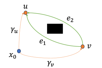
Figure 2: An example of edges with different homotopic traits

Fig. 2 is an example. While $\gamma_{v}\circ e_{1}\circ\gamma_{u}^{-1}$ is homotopic with the constant function, $\gamma_{v}\circ e_{2}\circ\gamma_{u}^{-1}$ is not due to the existence of the obstacle. Thus, $h(e_{1})$ is the unit and $h(e_{2})$ is the element corresponding to one counterclockwise turn around the obstacle. In the homotopy-augmented graph, two edges above $e_{1}$ and $e_{2}$ with the same source have different targets.

3.3 Presentation of Group

A presentation $\langle S|R\rangle$ of a group $G$ consists of a set $S\subseteq G$ of generators and a set $R$ of relations.

In the context of group theory, a word is a string consisting of generators and their inverses, which represents an element of the group. Relations are words that are considered equal to the identity element in the group.

$\langle S|R\rangle$ satisfies the following conditions.

• Any element of $G$ can be represented by a word formed from the generators in $S$ and their inverses.

• The kernel of the natural surjection from the free group $F_{S}$ on $S$ to $G$ is the smallest normal subgroup of $F_{S}$ containing $R$.

A relation $ab^{-1}\in R$ is sometimes denoted as $a=b$.

The decision problem of determining whether two given words represent the same element of the group is known as the word problem [61].

3.4 Braid Group

The configuration space $\mathcal{C}_{n}$ is defined as

$$\mathcal{C}_{n}:=\left\{(p_{1},p_{2},\ldots,p_{n})\in(\mathbb{R}^{2})^{n}\ \middle|\ p_{i}\neq p_{j}\text{ for all }i\neq j\right\}.$$ (4)

The $n$-th symmetric group $S_{n}$ naturally acts on $\mathcal{C}_{n}$ by permuting the indices. In the context of unlabeled multi-agent path planning, where we ignore the indices of agents, we consider the unlabeled configuration space $\mathcal{UC}_{n}$, which is defined as the quotient of $\mathcal{C}_{n}$ by $S_{n}$.

The fundamental group $\pi_{1}(\mathcal{UC}_{n})$ is known as the $n$-th braid group $B_{n}$. The fundamental group $\pi_{1}(\mathcal{C}_{n})$, which is a subgroup of $B_{n}$, is denoted as the $n$-th pure braid group $P_{n}$. There exists a natural surjective group homomorphism from $B_{n}$ to $S_{n}$, the kernel of which is $P_{n}$.

$B_{n}$ has a presentation given by

$$\langle\sigma_{1},\ldots,\sigma_{n-1}\ |\ \sigma_{i}\sigma_{j}\sigma_{i}^{-1}\sigma_{j}^{-1},\ \sigma_{i}\sigma_{i+1}\sigma_{i}\sigma_{i+1}^{-1}\sigma_{i}^{-1}\sigma_{i+1}^{-1}\rangle,$$ (5)

where $1\leq i<n-1$ and $i+1<j\leq n-1$ [63].

4 Method

We consider homotopy-aware multi-agent path planning with $n$ agents in the plane with no obstacles. We assume that a graph $G=(V,E)$ lying on $\mathbb{R}^{2}$ is given as a roadmap. When starts $s_{1},\ldots,s_{n}\in V$ and goals $g_{1},\ldots,g_{n}\in V$ are given, we want to find multiple solutions of multi-agent pathfinding problem on $G$ belonging to different homotopy classes as paths of the configuration space $\mathcal{C}_{n}$. Note that, since sizes of agents do not matter to homotopy when there are no obstacles, we can consider agents as points while calculating homotopy classes.

4.1 Reduction to Unlabeled Case

As mentioned earlier, in labeled multi-agent path planning, we can calculate homotopy classes as the unlabeled multi-agent path planning. To formalize this reduction, let $G^{n}=(V^{n},E^{n})$ be the $n$-times direct product of $G$ minus collision parts, which is a graph on the configuration space $\mathcal{C}_{n}$. We construct a graph $(V^{n}_{h},E^{n}_{h})$ as follows instead of using the homotopy-augmented graph for $\mathcal{C}_{n}$.

• $V^{n}_{h}:=V^{n}\times\pi_{1}(\mathcal{UC}_{n})=V^{n}\times B_{n}$.

• For each edge $e\in E^{n}$ from vertex $v\in V^{n}$ to vertex $u\in V^{n}$, and for each element $\alpha\in B_{n}$, $E^{n}_{h}$ contains an edge from $(v,\alpha)$ to $(u,\alpha h(\overline{e}))$, where $\overline{e}$ is the projection of $e$ to $\mathcal{UC}_{n}$ by the natural surjection, and $h(\overline{e})$ is calculated using the method described in § 4.2.

It is important to note that, for a specific multi-agent path planning task, it is not necessary to construct the entire graph, as it is not connected. Instead, we can focus on the relevant connected components of the graph. For example, for any vertex $v\in V^{n}$ and elements $\alpha,\beta\in B_{n}$, the connected components of $(v,\alpha)$ and $(v,\beta)$ are different unless $\alpha^{-1}\beta\in P_{n}$.

With our approach, we represent the homotopy classes of solutions for a specific instance of labeled multi-agent path planning problem by labeling them with elements in a coset of the pure braid group, instead of those in the pure braid group. The choice of coset depends on the relative positions of the agents’ start and goal locations. For a detailed explanation of why we do not use the pure braid group, see Appendix A.

4.2 Word Construction

The construction of words for $\mathcal{UC}_{n}$ is classically known [26].

Let $p_{1}=(x_{1},y_{1}),\ldots,p_{n}=(x_{n},y_{n})$ be the natural coordination of $\mathcal{C}_{n}$. We define:

$$\lambda_{2n}:=\{x_{1}<x_{2}<\cdots<x_{n}\},$$ (6)

$$\lambda^{2n-1}_{i}:=\{x_{1}<\cdots<x_{i}=x_{i+1}<\cdots<x_{n},y_{i}<y_{i+1}\},$$ (7)

for $1\leq i<n$. It is easy to see that the map $\lambda^{2n}\cup\bigcup_{i}\lambda^{2n-1}_{i}\hookrightarrow\mathcal{C}_{n}\twoheadrightarrow\mathcal{UC}_{n}$ is injective. We identify $\lambda^{2n},\lambda^{2n-1}_{i}$ with their images. $\mathcal{UC}_{n}\setminus\lambda^{2n}$ is $(2n-1)$-dimensional and $\mathcal{UC}_{n}\setminus\lambda^{2n}\setminus\bigcup_{i}\lambda^{2n-1}_{i}$ is $(2n-2)$-dimensional.

For simplicity, we assume that all $v\in V^{n}$ lie on $\lambda^{2n}$. We also choose a base point $x_{0}$ of the fundamental group within $\lambda^{2n}$. To make the homotopy-augmented graph explicit, we choose the standard path connecting $x_{0}$ and vertices of $V^{n}$ in $\lambda^{2n}$. The generator $\sigma_{i}$ of $\pi_{1}(\mathcal{UC}_{n})=B_{n}$ is represented by a loop in $\lambda^{2n}\cup\lambda^{2n-1}_{i}$ which traverses $\lambda^{2n-1}_{i}$ exactly once with the direction from region $\{y_{i}<y_{i+1}\}$ to region $\{y_{i}>y_{i+1}\}$. Consequently, for an edge $e$ on $\mathcal{UC}_{n}$, the word representing the corresponding braid $h(e)$ is constructed by detecting the traverses of $e$ with $\lambda^{2n-1}_{1},\ldots,\lambda^{2n-1}_{n-1}$. By examining the intersections of the boundaries of $\lambda^{2n-1}_{1},\ldots,\lambda^{2n-1}_{n-1}$, we obtain the relations $\sigma_{i}\sigma_{j}=\sigma_{j}\sigma_{i}$ for $i+1<j$ and $\sigma_{i}\sigma_{i+1}\sigma_{i}=\sigma_{i+1}\sigma_{i}\sigma_{i+1}$. The detailed derivation of these relations are omitted for brevity.

Intuitively, this construction can be described as follows. We arrange the agents in ascending order of their $x$-coordinates. $\sigma_{i}$ corresponds to the counterclockwise swap (Fig. 1(a)) of the $i$-th agent and $(i+1)$-th agent, and $\sigma_{i}^{-1}$ corresponds to their clockwise swap (Fig 1(b)). The word for an edge is constructed by detecting the swaps of agent indexes. The graphical explanation for the relations is shown in Fig. 3. The key observation is that the order in which the agents move does not affect the homotopy class. Therefore, we have the relations: (a) $\sigma_{i}\sigma_{j}=\sigma_{j}\sigma_{i}$ and (b) $\sigma_{i}\sigma_{i+1}\sigma_{i}=\sigma_{i+1}\sigma_{i}\sigma_{i+1}$.

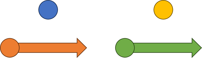
(a)

(b)

Figure 3: Figures illustrates relations. In both cases, red agent represents $i$-th agent, and green agent represents either $j$-th agent ($j>i+1$, in (a)) or $(i+1)$-th agent (in (b)). Movement of agents is depicted with arrows.

4.3 Dehornoy Order

In the above presentation of the braid group, the words are referred to as braid words. A braid word $w$ is considered reduced if it is an empty string or its main generator, which is the generator with the lowest index appearing in $w$, occurs only positively as $\sigma_{i}$ or only negatively as $\sigma_{i}^{-1}$ in $w$. It has been proven that no nonempty reduced braid word represents the identity element, and any word can be represented by a reduced braid word.

The Dehornoy order is a linear order on the braid group and defined as follows. For two braids $\alpha$ and $\beta$, we say $\alpha<\beta$ if $\alpha^{-1}\beta$ has a representation by a reduced word, the main generator of which occurs positively.

To obtain an algorithm for comparing braids, it suffices to construct a method for transforming given braid words into reduced braid words. Dehornoy [19] proposed an efficient algorithm for this purpose, known as the handle reduction method.

A $\sigma_{i}$-handle refers to a braid word of the form $\sigma_{i}^{e}v\sigma_{i}^{-e}$, where $e\in\{1,-1\}$ and $v$ contains no $\sigma_{i-1}^{\pm 1}$ nor $\sigma_{i}^{\pm 1}$. A $\sigma_{i}$-handle is permitted if it contains no $\sigma_{i+1}$-handle as a subword. A braid word is reduced if and only if it contains no permitted handle.

Consider the permitted $\sigma_{i}$-handle

$$\sigma_{i}^{e}v_{1}\sigma_{i+1}^{d}v_{2}\ldots\sigma_{i+1}^{d}v_{m}\sigma_{i}^{-e},$$ (8)

where $e,d\in\{1,-1\}$ and $v_{1},v_{2},\ldots,v_{m-1},v_{m}$ contain no $\sigma_{i-1}^{\pm 1}$, $\sigma_{i}^{\pm 1}$, nor $\sigma_{i+1}^{\pm 1}$. One step of handle reduction transforms this to

$$v_{1}\sigma_{i+1}^{-e}\sigma_{i}^{d}\sigma_{i+1}^{e}v_{2}\ldots\sigma_{i+1}^{-e}\sigma_{i}^{d}\sigma_{i+1}^{e}v_{m}.$$ (9)

In this transformation, $\sigma_{i}^{\pm e}$ is removed, and $\sigma_{i+1}^{d}$ is transformed to $\sigma_{i+1}^{-e}\sigma_{i}^{d}\sigma_{i+1}^{e}$. All other generators remain the same. The handle reduction method continues to apply these transformations to permitted handles contained in the given braid until a reduced braid word is obtained. This reduced braid word represents the same braid as the original word.

The time and space complexity of the handle reduction method with respect to the length of the braid word is conjectured to be quadratic and linear, respectively. [20].

4.4 Revised Prioritized Planning

We adopt revised prioritized planning (RPP) [17] for pathfinding. As classical prioritize planning, we fix a predetermined priority order for the agents and proceed to plan their paths one by one, avoiding collisions with the paths of previously planned agents. In RPP, in addition, the start positions of agents that have not yet been planned are also avoided, ensuring the completeness of the planning process under certain assumptions.

Algorithm 1 Homotopy-Aware RPP

1:Input a graph $G=(V,E)$

2:Input starts and goals $(s_{1},g_{1}),\ldots,(s_{n},g_{n})$

3:$\mathit{plans}\leftarrow\{\emptyset\}$

4:for $i=1,\ldots,n$ do

5:     $\mathit{Open},\mathit{Closed}\leftarrow\emptyset,\emptyset$

6:     Initialize a map $D$

7:     for $\mathit{plan}\in\mathit{plans}$ do

8:         Construct timed graph $G_{\mathit{plan}}=\left(V_{\mathit{plan}},E_{\mathit{plan}}\right)$

9:         Insert $(\mathit{plan},s_{\mathit{plan}},\varepsilon)$ to $\mathit{Open}$

10:         $D[\mathit{plan},s_{\mathit{plan}},\varepsilon]\leftarrow 0$

11:     end for

12:     $\mathit{newplans}\leftarrow\emptyset$

13:     while $\mathit{Open}\neq\emptyset$ do

14:         Pop $(\mathit{plan},v,w)$ from $\mathit{Open}$

15:         Insert $(\mathit{plan},v,w)$ to $\mathit{Closed}$

16:         if $v=g_{\mathit{plan}}$ then

17:              Reconstruct path $p$ of agent $i$

18:              Insert $\mathit{plan}\cup p$ to $\mathit{newplans}$

19:              if enough plans are found then

20:                  break

21:              end if

22:         end if

23:         for edge $e\in E_{\mathit{plan}}$ from $v$ do

24:              $v^{\prime}\leftarrow\mathrm{target}(e)$

25:              $w^{\prime}\leftarrow\mathrm{NextBraid}(\mathit{plan},e,w)$

26:              $d^{\prime}\leftarrow D[\mathit{plan},v,w]+\mathrm{length}(e)$

27:              if $(\mathit{plan},v^{\prime},w^{\prime})\notin\mathit{Open}\cup\mathit{Closed}$ then

28:                  $D[\mathit{plan},v^{\prime},w^{\prime}]\leftarrow d^{\prime}$

29:                  Insert $(\mathit{plan},v^{\prime},w^{\prime})$ to $\mathit{Open}$

30:              else if $D[\mathit{plan},v^{\prime},w^{\prime}]>d^{\prime}$ then

31:                  $D[\mathit{plan},v^{\prime},w^{\prime}]\leftarrow d^{\prime}$

32:              end if

33:         end for

34:     end while

35:     $\mathit{plans}\leftarrow\mathit{newplans}$

36:end for

37:return $\mathit{plans}$

Alg. 1 presents the pseudocode of our homotopy-aware version of RPP which generates homotopically distinct solutions. The notation $\varepsilon$ denotes the empty braid word. At line 8, we construct a graph $G_{\mathit{plan}}$, which is created by adding a time dimension to $G$ and removing parts colliding with $plan$, using a method by Silver [68] or by Phillips and Likhachev [62]. In this construction, we also remove $s_{i+1},\ldots,s_{n}$ from $G_{\mathit{plan}}$. In the following lines, $s_{\mathit{plan}}$ and $g_{\mathit{plan}}$ denote the vertices corresponding to the start, which is $s_{i}$ with time $0$, and the goal, which is $g_{i}$ with late enough time, respectively. At line 14, the popped element $(\mathit{plan},v,w)$ is selected as that with the minimum $\mathrm{cost}(\mathit{plan})+D[\mathit{plan},v,w]+h(v,g_{\mathit{plan}})$, where $h$ is the heuristic function. The function $\mathrm{NextBraid}(\mathit{plan},e,w)$ at line 25 calculates the braid word after the agent $i$ moves along $e$ and the agents from $1$ to $i-1$ move in accordance with $\mathit{plan}$ using the method explained in § 4.2. The algorithm presented in § 4.3 is used to manage $\mathit{Open}$, $\mathit{Closed}$, and $D$. Thanks to the Dehornoy order, we can efficiently maintain them by using a data structure such as self-balancing binary search trees. For simplicity, we omit the details on path reconstruction.

Note that, by A* searching the homotopy-augmented graph, we can also solve the $k$-shortest non-homotopic path planning [9, 77]. However, since the runtime of A* search grows rapidly with respect to the number of agents, we do not adopt it.

To facilitate the word construction method in grid environments, we introduce a virtual slightly inclined x-axis, such that for any two grid cells $(i,j)$ and $(k,l)$, cell $(i,j)$ has a smaller x-coordinate than cell $(k,l)$ if and only if $i<k$ or $i=k,j<l$. For grid cases, the following proposition holds.

Proposition 1.

Under the following conditions:

• $G$ is a four-connective grid graph

• no start grid or goal grid lies on boundary grids

• no two start grids or two goal grids are adjacent vertically, horizontally, or diagonally

• for any $1\leq i<j\leq n$, $g_{i}$ and $s_{j}$ are not adjacent vertically, horizontally, or diagonally

Alg. 1 can provide a solution belonging to any homotopy class.

For the proof, refer to Appendix B.

5 Experiments

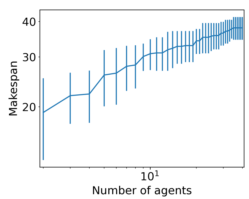
(a) Makespan of the first solution

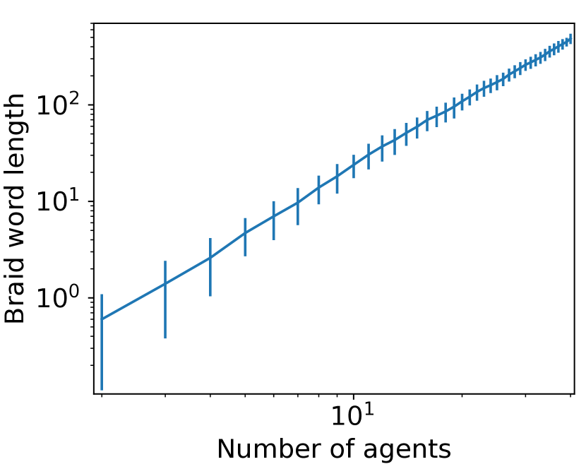
(b) Length of the first braid word

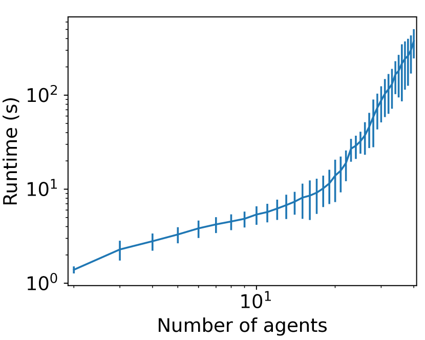
(c) Runtime to generate $100$ solutions

Figure 4: Log-log plots of results averaged over $10$ instances. Error bars show standard derivation.

We conducted two experiments. In the first experiment, we measured the runtime of our approach to assess its efficiency and scalability. In the second experiment, our focus was to demonstrate the effectiveness of generating homotopically distinct coarse solutions for planning low-cost trajectories. We demonstrated how our approach can lead to improved trajectories by comparing the results obtained after optimization.

The codes used for these experiments are available at https://github.com/omron-sinicx/homotopy-aware-MAPP.

5.1 Problem Setting and Implementation

For both experiments, we used problem instances of multi-agent pathfinding on grids. In the problem setting, we enforced restrictions to prevent vertex conflicts, where two agents occupy the same grid cell, and following conflicts, where one agent moves to a grid cell immediately left by another agent at the same time [70]. To ensure the fulfillment of the conditions specified in Proposition 1, we make sure to generate problem instances such that the start and goal positions did not lie on boundary grids, and no two were adjacent vertically, horizontally, or diagonally.

In our implementation, we construct $G_{\mathit{plan}}$ as a three-dimensional grid following the approach used by Silver [68]. We precompute the minimum distance to $g_{\mathit{plan}}$ for all vertices of $G_{\mathit{plan}}$ and adopt it as the heuristic function $h$. Line 19 of Alg. 1 checks whether the desired number ($K$) of solutions has been found. We use the ”FullHRed” algorithm [19] as a specific strategy for the handle reduction method, which selects the handle with the leftmost right end to reduce and reduces the braid word as a word of the free group after each handle reduction step. Our implementation is conducted in C++, and we use the priority queue and map data structures from the standard library to manage $\mathit{Open}$, $\mathit{Closed}$, and $D$.

5.2 Evaluation of Runtime

We evaluated the runtime performance using random instances of the multi-agent pathfinding problem. We generated $10$ instances with $40$ agents on a $29\times 29$ grid graph, adhering to the constraints mentioned earlier. For each instance, we ran our method with the objective of finding $100$ solutions. The runtime from the beginning was measured after each agent’s planning-process completion (line 35 at Alg.1). We also recorded the makespan and length of the braid word for the first generated solution at the same time. Intel Core i9-9900K CPU and 32GB RAM are utilized for this experiment. We conducted this experiment on Ubuntu 20.04 via Windows Subsystem for Linux 2.

Fig. 4 illustrates the results.

We observed that the braid length is approximately proportional to the square of the number of agents. This was expected, as each element in the braid word corresponds to swapping adjacent agents, and the expected inversion number of a randomly shuffled sequence is proportional to the square of its length.

We noticed that runtime is approximately proportional to the fifth power of the number of agents when that number is large enough. The size of $G_{\mathit{plan}}$ is bounded by the product of the size of the grid map and the makespan of plans, which increases at a slow enough rate to be negligible. Hence, the primary factor contributing to the growth in runtime is expected to be the handle reduction process. Since the complexity of the handle reduction method is conjectured to be quadratic with respect to the braid word length, we expect the runtime of planning for the $i$-th agent to be $O(i^{4})$. This justifies the observed quintic increase in the total runtime.

5.3 Optimization Experiment

5.3.1 Generating initial plans

We conducted the optimization experiment using $100$ random instances of multi-agent pathfinding problems with $10$ agents on a $14\times 14$ grid graph, following the aforementioned constraints. For each instance, we generated $100$ solutions using our method with $K=100$.

We also generated solutions using the following two approaches as baseline methods:

• Optimal One (OO): We generate one optimal solution on the grid for each instance.

• Revised prioritized planning with various priority orders (PPvP): We generate $100$ solutions for each instance by revised prioritized planning with randomly selected priority orders.

5.3.2 Optimization

After generating the initial solutions, we proceeded to optimize them. Let $\gamma_{1},\ldots,\gamma_{n}$ be the trajectories of the agents. The cost function $C$ is defined as

$$C(\gamma_{1},\ldots,\gamma_{n}):=\frac{1}{2}\sum_{i}\int_{0}^{1}\left\|\frac{d^{2}\gamma_{i}}{dt^{2}}(t)\right\|^{2}dt+c_{\mathrm{c}}\sum_{i\neq j}\int_{0}^{1}\max\left\{\frac{1}{\left\|\gamma_{i}(t)-\gamma_{j}(t)\right\|}-\frac{1}{2r},0\right\}^{2}dt$$ (10)

with constraints

$$\frac{d\gamma_{i}}{dt}(0)=\frac{d\gamma_{i}}{dt}(1)=\mathbf{0},$$ (11)

where $c_{\mathrm{c}}$ is a penalty coefficient and $r=0.5$ is the collision radius of agents. The first term represents a smoothness cost [80], while the second term represents a collision penalty [40].

To carry out trajectory optimization, we approximated trajectories using timed waypoints and used the Levenberg-Marquardt algorithm [49, 54]. For further details on the optimization process, refer to Appendix C.

5.3.3 Results

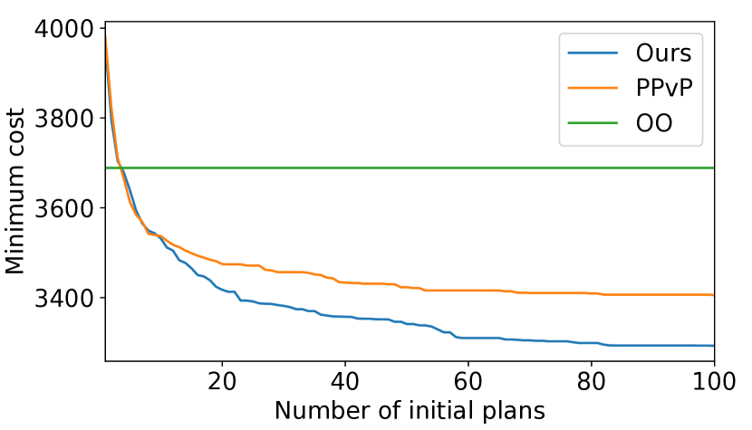
Figure 5: The minimum cost of plans after optimization among the first $N$ generated plans, averaged over 100 instances, with respect to $N$

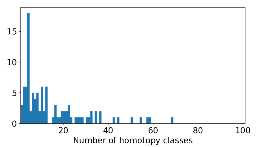
Figure 6: The number of homotopy classes present in $100$ solutions generated with PPvP for each $100$ instances

In Fig. 6, for each value of $N=1,\ldots,100$ on the x-axis, the blue curve (Ours) and the orange curve (PPvP) represent the cost of the best plan obtained from optimizing the first $N$ initial plans, averaged over 100 instances. The green line (OO) represents the cost of optimization of the optimal plan on grid, also averaged over 100 instances. While OO yielded better trajectories when only a few initial solutions are considered, as the number of initial plans increased, the minimum cost decreased, and the rate of decrease was faster with our method than with PPvP.

We analyzed the number of homotopically distinct solutions generated with PPvP for each instance and created a histogram, as shown in Fig. 6. The results indicate that this naive approach failed to generate numerous homotopically distinct solutions in the vast majority of instances.

6 Conclusion and Future Work

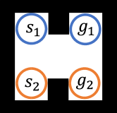
Figure 7: Example scenarios in which homotopy depends on order in which agents pass through a narrow part

We proposed a practical method for multi-agent path planning in the plane. We used the Dehornoy order and revised prioritized planning to efficiently generate homotopically distinct plans. Our experimental results indicate that the runtime of our method increases approximately quintically with respect to the number of agents. We also conducted an experiment to optimize the generated plans and compared them with those generated with baseline methods. The results indicated that generating homotopically distinct plans using our method led to improvement of optimized plans. This showcases the effectiveness of our approach in achieving lower-cost trajectories for multi-agent path planning.

One of the main limitations of our approach is the assumption that the plane has no obstacles. In scenarios where several agents need to pass through a narrow part where only one agent can go at a time, homotopy classes of solutions can split, depending on the order in which the agents pass through the narrow section. Fig. 7 illustrates such a situation, where the homotopy classes of solutions depend on whether the first agent goes through the narrow section earlier or the second agent does. This phenomenon does not occur when the size of agents can be ignored, as assumed with our approach.

Another limitation is the abandonment of optimality. While simple A* search is workable, it becomes impractical for larger problem instances [69]. To improve efficiency without sacrificing optimality, it may be possible to combine our framework with efficient optimal approaches. To calculate braids while searching, it is required to determine the moves of all agents. This makes it challenging to use conflict-based search, where agent paths are planned independently in its low-level search. On the other hand, increasing-cost tree search could be a more suitable candidate since it takes into account combinations of all agent paths in its low-level search. Another non-trivial challenge is to make reduction-based methods homotopy-aware.

The time complexity of the comparison algorithm for the Dehornoy order can be a limitation when dealing with a large number of agents. To treat hundreds or thousands of agents, the development of an efficient hash function for braids would be beneficial. Lawrence-Krammer representation is a faithful representation of braid groups [14, 44]. Although directly using this representation may not be practical due to its high dimensionality, it has the potential for constructing a suitable hash function for braids.

A potential extension of our research involves exploring decentralized control strategies. Specifically, it may be possible to achieve effective coordination among agents with minimal communication by conveying only braids to other agents.

Appendix A On Presentations of the Pure Braid Groups

Bhattacharya and Ghrist [9] gave a presentation of the homotopy group for path planning with $n$ agents in the plane, which is the pure braid group $P_{n}$, with the following generators:

$$\left\{u_{i,j/\gamma_{i+1},\ldots,\gamma_{j-1}}\middle|1\leq i<j\leq n,\,\gamma_{i+1},\ldots,\gamma_{j-1}\in\{+,-\}\right\}.$$ (12)

The relations are as follows.

• For $i<j<k$, $\alpha_{i+1},\ldots,\alpha_{j-1}\in\{+,-\}$, and $\beta_{j+1},\ldots,\beta_{k-1}\in\{+,-\}$,

  $$\begin{split}&u_{i,j/\alpha_{i+1},\ldots,\alpha_{j-1}}\cdot u_{i,k/\alpha_{i+1},\ldots,\alpha_{j-1},-,\beta_{j+1},\ldots,\beta_{k-1}}\cdot u_{j,k/\beta_{j+1},\ldots,\beta_{k-1}}\\ &\cdot u^{-1}_{i,j/\alpha_{i+1},\ldots,\alpha_{j-1}}\cdot u^{-1}_{i,k/\alpha_{i+1},\ldots,\alpha_{j-1},+,\beta_{j+1},\ldots,\beta_{k-1}}\cdot u^{-1}_{j,k/\beta_{j+1},\ldots,\beta_{k-1}},\end{split}$$ (13)

  $$\begin{split}&u_{i,j/\alpha_{i+1},\ldots,\alpha_{j-1}}\cdot u_{i,k/\alpha_{i+1},\ldots,\alpha_{j-1},-,\beta_{j+1},\ldots,\beta_{k-1}}\cdot u^{-1}_{i,j/\alpha_{i+1},\ldots,\alpha_{j-1}}\cdot u^{-1}_{i,k/\alpha_{i+1},\ldots,\alpha_{j-1},+,\beta_{j+1},\ldots,\beta_{k-1}},\end{split}$$ (14)

  and

  $$\begin{split}&u_{i,k/\alpha_{i+1},\ldots,\alpha_{j-1},-,\beta_{j+1},\ldots,\beta_{k-1}}\cdot u_{j,k/\beta_{j+1},\ldots,\beta_{k-1}}\cdot u^{-1}_{i,k/\alpha_{i+1},\ldots,\alpha_{j-1},+,\beta_{j+1},\ldots,\beta_{k-1}}\cdot u^{-1}_{j,k/\beta_{j+1},\ldots,\beta_{k-1}}.\end{split}$$ (15)

• Let $i,j,i^{\prime},j^{\prime}$ be distinct indices with $i<j,i^{\prime}<j^{\prime},i<i^{\prime}$. Let $\gamma_{i+1},\ldots,\gamma_{j-1}\in\{+,-\}$ and $\gamma^{\prime}_{i^{\prime}+1},\ldots,\gamma^{\prime}_{j^{\prime}-1}\in\{+,-\}$ be signs. When $i<i^{\prime}<j<j^{\prime}$, we assume that $\gamma_{i^{\prime}}\neq\gamma^{\prime}_{j}$ and $(\gamma_{k},\gamma^{\prime}_{k})\neq(-\gamma_{i^{\prime}},\gamma_{i^{\prime}})$ for all $i^{\prime}<k<j$. When $i<i^{\prime}<j^{\prime}<j$, we assume that $\gamma_{i^{\prime}}=\gamma_{j^{\prime}}$ and $(\gamma_{k},\gamma^{\prime}_{k})\neq(-\gamma_{i^{\prime}},\gamma_{i^{\prime}})$ for all $i^{\prime}<k<j^{\prime}$. For such tuples,

  $$\begin{split}&u_{i,j/\gamma_{i+1},\ldots,\gamma_{j-1}}\cdot u_{i^{\prime},j^{\prime}/\gamma^{\prime}_{i^{\prime}+1},\ldots,\gamma^{\prime}_{j^{\prime}-1}}\cdot u^{-1}_{i,j/\gamma_{i+1},\ldots,\gamma_{j-1}}\cdot u^{-1}_{i^{\prime},j^{\prime}/\gamma^{\prime}_{i^{\prime}+1},\ldots,\gamma^{\prime}_{j^{\prime}-1}}.\end{split}$$ (16)

The description in the original paper is incomplete as it omits the condition for the relation (16).

We consider a word

$$w=u_{1,4/--}u_{2,4/-}u_{3,4}u_{1,4/++}^{-1}u_{2,4/+}^{-1}u_{3,4}^{-1},$$ (17)

which is irreducible by using Dehn’s algorithm. On the other hand,

$$\begin{split}w&=u_{2,4/-}u_{1,4/+-}u_{3,4}u_{1,4/++}^{-1}u_{2,4/+}^{-1}u_{3,4}^{-1}\\ &=u_{2,4/-}u_{3,4}u_{2,4/+}^{-1}u_{3,4}^{-1}\\ &=u_{3,4}u_{3,4}^{-1}\\ &=e,\end{split}$$ (18)

where the first, second, and third equalities are deduced from (15) with $(i,j,k)=(1,2,4),(1,3,4),(2,3,4)$ respectively. Thus, Dehn’s algorithm is incomplete for this presentation when $n\geq 4$.

The pure braid group $P_{n}$ has a standard presentation [63] with generators $\left\{a_{i,j}\middle|1\leq i<j\leq n\right\}$, where

$$\begin{split}a_{i,j}:=&\sigma_{j-1}\sigma_{j-2}\cdots\sigma_{i+1}\sigma_{i}^{2}\sigma_{i+1}^{-1}\cdots\sigma_{j-2}^{-1}\sigma_{j-1}^{-1}=\sigma_{i}^{-1}\sigma_{i+1}^{-1}\cdots\sigma_{j-2}^{-1}\sigma_{j-1}^{2}\sigma_{j-2}\cdots\sigma_{i+1}\sigma_{i},\end{split}$$ (19)

and the following relations.

• For $1\leq i<j<k\leq n$,

  $$a_{i,j}a_{i,k}a_{j,k}a_{i,j}^{-1}a_{j,k}^{-1}a_{i,k}^{-1},$$ (20)

  $$a_{i,k}a_{j,k}a_{i,j}a_{i,k}^{-1}a_{i,j}^{-1}a_{j,k}^{-1}.$$ (21)

• For $1\leq i<j<k<l\leq n$,

  $$a_{i,j}a_{k,l}a_{i,j}^{-1}a_{k,l}^{-1},$$ (22)

  $$a_{i,l}a_{j,k}a_{i,l}^{-1}a_{j,k}^{-1},$$ (23)

  and

  $$a_{i,k}a_{j,k}a_{j,l}a_{j,k}^{-1}a_{i,k}^{-1}a_{j,k}a_{j,l}^{-1}a_{j,k}^{-1}.$$ (24)

When

$$u_{i,j/\sigma_{i+1},\ldots,\sigma_{j-1}}=a_{i,i+1}^{d_{i+1}}\cdots a_{i,j-1}^{d_{j-1}}a_{i,j}a_{i,j-1}^{-d_{j-1}}\cdots a_{i,i+1}^{-d_{i+1}},$$ (25)

where $d_{k}=1$ if $\sigma_{k}=+$ and $d_{k}=0$ if $\sigma_{k}=-$, the relations for $\{u_{i,j/\sigma_{i+1},\ldots,\sigma_{j-1}}\}$ can be deduced from the relations for $\{a_{i,j}\}$ and vice versa. Therefore, we can translate words from Bhattacharya’s presentation to words for the standard presentation. However, this translation increases the lengths of words by a factor of $O(n)$. To the best of our knowledge, there is no algorithm for the word problem of the pure braid group that is efficient enough to compensate for these drawbacks. This is why we use elements of the braid group to label homotopy classes, instead of those of the pure braid group.

Appendix B Proof of Proposition 1

Lemma 1.

For $1\leq k\leq n$, let $F_{k}:P_{n}\rightarrow P_{n-1}$ be the projection forgetting the $k$-th strand. Its kernel is generated by $a_{1,k},a_{2,k},\ldots,a_{k-1,k}$ and $a_{k,k+1},a_{k,k+2},\ldots,a_{k,n}$ with the notation in Appendix A.

Proof.

This is true for $k=n$ [63]. For arbitrary $k$, let $b_{k}:=\sigma_{n-1}\sigma_{n-2}\cdots\sigma_{k}\in B_{n}$. Since $P_{n}$ is a normal subgroup, the conjunction by $b_{k}$ maps $P_{n}$ to $P_{n}$. Furthermore, $F_{k}(\alpha)=F_{n}(b_{k}\alpha b_{k}^{-1})$. Thus, the kernel of $F_{k}$ is generated by $b_{k}^{-1}a_{1,n}b_{k},\ldots,b_{k}^{-1}a_{n-1,n}b_{k}$. However,

$$b_{k}^{-1}a_{i,n}b_{k}=\begin{cases}a_{i,k}&\text{if $i<k$}\\ a_{k,i+1}&\text{if $i\geq k$}.\end{cases}$$ (26)

∎

We consider a problem instance $(s_{1},g_{1}),\ldots,(s_{n},g_{n})$ satisfying the assumption and a braid $\alpha\in B_{n}$ corresponding to one of its solutions. For $1\leq 1\leq n$, let $\alpha_{i}\in B_{i}$ be the braid corresponding to the paths for the first $i$ agents in $\alpha$. We prove that our method can generate a solution $p_{i}$ in the homotopy class corresponding to $\alpha_{i}$ by induction for $i$. When $i=1$, this is clear.

For $i>1$, by the assumption of the problem instance, the $i$-th agent can reach its goal after agents from $1$ to $i-1$ have finished, while avoiding the goal positions $g_{1},\ldots,g_{i-1}$ and the start positions $s_{i+1},\ldots,s_{n}$. Therefore, we can generate a plan $p_{i}^{\prime}$ for the first $i$ agents on the basis of $p_{i-1}$. Let $\beta_{i}\in B_{i}$ be the braid corresponding to $p_{i}^{\prime}$.

To construct the desired plan, we need to add the moves of the $i$-th agent to $p_{i}^{\prime}$ after the agents from $1$ to $i-1$ have reached their goals. These moves must correspond to the braid $\beta_{i}^{-1}\alpha_{i}\in P_{i}$. Let $c_{1},\ldots,c_{i}$ be $g_{1},\ldots,g_{i}$ sorted by their $x$-coordinates, and suppose $g_{i}=c_{k}$. Since $\alpha_{i}$ and $\beta_{i}$ coincide when the $i$-th agent is forgotten, $\beta_{i}^{-1}\alpha_{i}$ is in the kernel of $F_{k}$, which is generated by $a_{1,k},\ldots,a_{k-1,k},a_{k,k+1},\ldots,a_{k,n}$ in accordance with Lemma 1.

Thus, it is sufficient to demonstrate that, after all agents have reached their goals, the $i$-th agent can move to construct any of $a_{1,k},\ldots,a_{k-1,k},a_{k,k+1},\ldots,a_{k,n}$ and their inverses, while avoiding $g_{1},\ldots,g_{i-1}$ and $s_{i+1},\ldots,s_{n}$. Fig. 8 illustrates a construction of such paths. The agent initially positioned at $c_{k}$ moves to $c_{j}$ along a path with a high $y$-coordinate, circumvents $c_{j}$, and then returns to $c_{k}$ using the same path. If the agent moves around the $c_{j}$ counterclockwise, the homotopy corresponds to $a_{j,k}$ or $a_{k,j}$ and if the agent moves clockwise, it corresponds to their inverses. When $j<k$, the braid for this loop is given by:

$$\sigma_{k-1}\cdots\sigma_{j+1}\sigma_{j}^{\pm 2}\sigma_{j+1}^{-1}\cdots\sigma_{k-1}^{-1}=a_{j,k}^{\pm 1}.$$ (27)

Similarly, when $j>k$, it is given by:

$$\sigma_{k}^{-1}\ldots\sigma_{j-2}^{-1}\sigma_{j-1}^{\pm 2}\sigma_{j-2}\ldots\sigma_{k}=a_{k,j}^{\pm 1}.$$ (28)

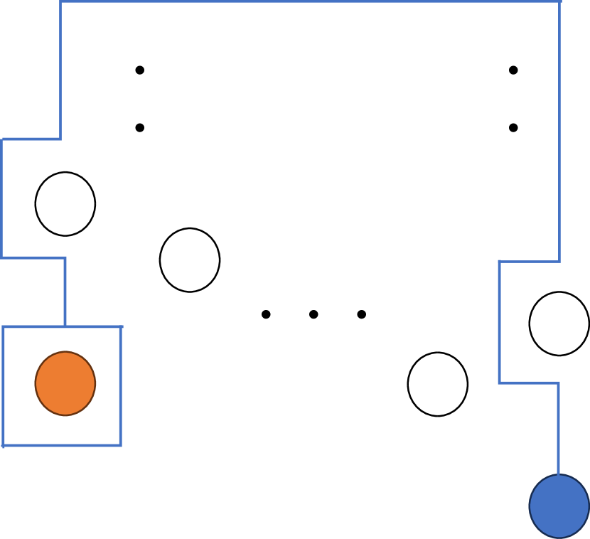
(a) $j<k$

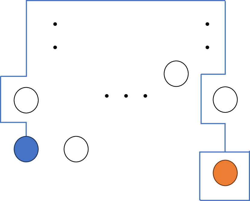
(b) $k<j$

Figure 8: Paths with homotopy corresponding to $a_{j,k},a_{k,j}$ or their inverses. The blue circle means $g_{i}=c_{k}$ and the orange circle means $c_{j}$. White circles mean other $c_{1},\ldots,c_{i}$ or $s_{i+1},\ldots,s_{n}$.

Appendix C Details of Optimization

We approximate the trajectories of the $i$-th agent by $(K+1)$ timed waypoints $(p_{i,0},0),(p_{i,1},1/K),\ldots,(p_{i,K},1)$ with $p_{i,0}=s_{i}$ and $p_{i,K}=g_{i}$, where $K=100$. The cost function is then reformulated as

$$\begin{split}C(p_{1,0},\ldots,p_{1,K},p_{2,0},\ldots,p_{n,K}):=&\frac{K^{3}}{2}\sum_{i}\sum_{k=0}^{K}\left\|p_{i,k+1}+p_{i,k-1}-2p_{i,k}\right\|^{2}\\ &+\frac{c_{\mathrm{c}}}{K}\sum_{i\neq j}\sum_{k=0}^{K}\max\left\{\frac{1}{\left\|p_{i,k}-p_{j,k}\right\|}-\frac{1}{2r},0\right\}^{2},\end{split}$$ (29)

where $p_{i,-1}:=p_{i,0}$ and $p_{i,K+1}:=p_{i,K}$.

We solved this continuous optimization problem with Levenberg-Marquardt algorithm implemented in g²o 1.0.0 [46].

The $p_{i,k}$ values are initialized by the initial plan on the grid. We optimize them by $10000$ steps of the Levenberg-Marquardt algorithm. The collision-penalty constant $c_{c}$ is initially set to $10000$ and multiplied by $1.001$ after every optimization step.

References

- Adler et al. [2015] Aviv Adler, Mark De Berg, Dan Halperin, and Kiril Solovey. Efficient multi-robot motion planning for unlabeled discs in simple polygons. In Algorithmic Foundations of Robotics XI: Selected Contributions of the Eleventh International Workshop on the Algorithmic Foundations of Robotics, pages 1–17. Springer, 2015.
- Andreychuk et al. [2022] Anton Andreychuk, Konstantin Yakovlev, Pavel Surynek, Dor Atzmon, and Roni Stern. Multi-agent pathfinding with continuous time. Artificial Intelligence, page 103662, 2022.
- Arias et al. [2021] Felipe Felix Arias, Brian Ichter, Aleksandra Faust, and Nancy M Amato. Avoidance critical probabilistic roadmaps for motion planning in dynamic environments. In IEEE International Conference on Robotics and Automation, pages 10264–10270, 2021.
- Artin [1947a] Emil Artin. Braids and permutations. Annals of Mathematics, pages 643–649, 1947a.
- Artin [1947b] Emil Artin. Theory of braids. Annals of Mathematics, pages 101–126, 1947b.
- Barták et al. [2017] Roman Barták, Neng-Fa Zhou, Roni Stern, Eli Boyarski, and Pavel Surynek. Modeling and solving the multi-agent pathfinding problem in picat. In 2017 IEEE 29th International Conference on Tools with Artificial Intelligence (ICTAI), pages 959–966. IEEE, 2017.
- Bespamyatnikh [2003] Sergei Bespamyatnikh. Computing homotopic shortest paths in the plane. Journal of Algorithms, 49(2):284–303, 2003.
- Bhattacharya [2010] Subhrajit Bhattacharya. Search-based path planning with homotopy class constraints. In Proceedings of the AAAI conference on artificial intelligence, volume 24, pages 1230–1237, 2010.