Dissipation-induced cooperative advantage in a quantum thermal machine

Abstract

We show that a quantum heat engine where the working medium is composed by two non-interacting quantum harmonic oscillators, connected to common baths via periodically modulated couplings, exhibits a cooperative advantage with respect to the case of two independent single-oscillator engines working in parallel. The advantage extends from weak to strong damping, being particularly evident in the latter case, where the independent engines cannot deliver any useful power, while the coupling to common baths allows for efficiency and power comparable and in some parameter regions even higher than those obtained in the limit of weak dissipation. The surprising fact that strong dissipation is a useful resource for a thermal machine is explained in terms of the appearance of a collective mode, with the two oscillators locked at a common, hybrid frequency, intermediate between their bare frequencies. Our results are first illustrated in the simplest case of monochromatic drivings and then corroborated after optimization over generic periodic driving protocols. Using machine learning tools, we perform an optimization over arbitrary driving protocols to find the Pareto front representing optimal tradeoffs between the power and the efficiency that the engine can deliver. Finally, we find a protocol to measure the entanglement established in the working medium via measurement of a small set of thermodynamic quantities, that is, the output work under specific driving protocols.

I Introduction

Huygens’ synchronization of two pendulum clocks mounted on a common support [1], Gulliver tied down by the Lilliputians [2], avian flocks [3], nuclear fission, ferromagnetism, and superconductivity are examples of cooperative phenomena, where the constituents of a system cannot be regarded as acting independently from each other. Concepts such as synchronization, self-organization, and phase separation are of interest not only for physics but also for biochemistry, engineering, economics, and sociology.

On the road to the development of quantum technologies [4], a fundamental question is whether there can be a quantum advantage when quantum correlations are established between the constituents of a system [5] (for instance, the qubits in a quantum computer). In the context of quantum thermal machines [6, 7, 8, 9, 10, 11, 12, 13, 14, 15, 17, 18], the question can be posed as follows: can a working medium (WM) made of $N$ constituents exhibit better performances than an array of $N$ independent engines working in parallel? If so, is the ensuing cooperative advantage of quantum nature or could it be found also for classical thermal machines? Furthermore, can dissipation be exploited to improve machine performance or does it play only a detrimental role? Even though previous investigations remarkably found parameter regions where collective advantage features occur [19, 20, 21, 22, 23, 24, 25, 26, 27, 28, 29], even related to damping induced phenomena [30, 31, 32, 33, 34, 35, 36, 37, 38], a complete answer to the above questions has not been reached yet. Moreover, given it’s difficulty, a systematic study comparing joint and independent thermal machines performing a full optimization over the driving protocol is still lacking. One strategy to tackle such a problem is to use machine learning-based techniques, which have been recently employed for the optimization of quantum heat engines [39, 42, 40, 41, 43, 44].

In this paper, we consider (see Fig. 1(a) for a schematic drawing of our model]) a WM composed of two non-interacting quantum harmonic oscillators (QHOs), coupled to common (hot and cold) baths, modeled, following the Caldeira-Leggett framework [45, 46, 47], as a collection of independent harmonic oscillators. Although the two QHOs do not directly interact with each other, non–trivial bath–mediated correlations can be established between them [30, 32]. The external driving of the machine occurs through generic periodic modulations of the couplings with one reservoir. Coupling modulation can be suitably engineered to perform thermodynamic tasks [48, 49, 50], and here we shall focus on the heat engine working mode.

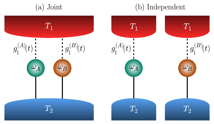
Figure 1: Sketch of the quantum thermal machines under study. (a) Two QHOs, with frequencies $\omega_{A}$ and $\omega_{B}$, are in contact with two common thermal reservoirs at temperatures $T_{\nu}$, with $\nu=1,2$. The WM exchanges heat currents $J_{\nu}$ with the reservoirs and total power $P$ generated by an external drive that periodically modulates the weak coupling with the $\nu=1$ reservoir (dashed lines). The $\nu=2$ WM-bath coupling is assumed static and much stronger (solid lines). (b) The two uncoupled QHOs in the same configuration as in Panel (a) but now in contact with independent thermal reservoirs. Here, no correlations are mediated by the baths, and the quantum thermal machine consists of independent two-terminal devices working in parallel.

We show that the baths mediate a cooperative advantage with respect to the case of independent heat engines (see Fig. 1(b)). Interestingly enough, the advantage is striking in the case of strong dissipation (strong static coupling to one bath), in which one would naively expect overdamped dynamics and poor performance of the engine. While this is the case for independent machines, for which the engine operating regime disappears, in the joint configuration the common baths sustain instead engine’s efficiency and power comparable or even better than those obtained in the limit of weak dissipation. We explain this surprising result in terms of the appearance, at strong damping, of a frequency- and phase- locked mode, for which the oscillators have a common, hybrid frequency, intermediate between their bare characteristic frequencies, and oscillate in phase opposition. This cooperative mode turns out to be only weakly damped, with damping time increasing with the dissipation strength.

Our results are first illustrated in the case of monochromatic drives, and then corroborated optimizing over arbitrary periodic drivings, without any a priori assumption on the shape or speed of the drivings. Furthermore, we characterize the heat engine performance in terms of both efficiency and extracted power. These quantities cannot be simultaneously optimized: indeed, high power engines typically exhibit a low efficiency, and vice-versa. We thus employ the concept of the Pareto front [51], recently employed in the context of quantum thermodynamics [52, 53, 54, 39, 40, 41], to find optimal tradeoffs between power and efficiency that the engine can deliver. The Pareto front is the set of all Pareto-optimal solutions (driving protocols), i.e. those where one cannot further improve one quantity without sacrificing the other. We point out that our calculations of the Pareto front extend machine learning tools to non-Markovian quantum thermodynamics, beyond the standard Lindblad approximation.

Finally, we have investigated whether there is a relationship between cooperative advantage and the establishment of non-classical correlations between the two QHOs, focusing on the logarithmic negativity [32, 58, 55, 56, 57] as a measure of entanglement. While we could not find a direct connection between entanglement and cooperative advantage, we obtained as an interesting byproduct a protocol to measure entanglement not via full quantum state tomography to reconstruct the system’s density matrix, but simply via a small number of measurements of thermodynamic quantities, more precisely of the output work under specific driving protocols.

The manuscript is organized as follows: Sec. II introduces the model under investigation and the thermodynamic quantities of interest. Sec. III focuses on the influence of bath-mediated interactions on thermodynamic quantities, discussing the behaviour of the response function, and illustrating the emergence of frequency locking and phase locking at strong damping. Sec. IV discusses the effects of bath-mediated correlations on the working regime of the quantum heat engine. Power performance enhancements, due to cooperative effects, are shown. Cooperative effects are most apparent in the regime of strong dissipation, when full frequency and phase locking is settled, with stable and sizeable output power. These results are corroborated by a complete driving-protocol optimization yielding the full Pareto front describing the power–efficiency trade–off. Finally, a direct link between entanglement and thermodynamic quantities, i.e., average work, at strong damping is discussed. Sec. V is devoted to the conclusions and perspectives; technical details can be found in various Appendices.

II Model and thermodynamic quantities

II.1 General setting

We consider a quantum thermal machine, where the WM is in contact with two reservoirs $\nu=1,2$ at temperatures $T_{1}$ and $T_{2}$, respectively. The WM is made of two uncoupled (no direct coupling) QHOs, labelled $l=A,B$, as sketched in Fig. 1(a). This configuration, dubbed joint, will be compared with the one sketched in Fig. 1(b), where two independent QHOs work in a parallel configuration with separate baths. We assume that the WM-bath couplings with the $\nu=1$ reservoir are weak and governed by a time-dependent modulation [48, 49, 50]

$$g_{1}^{(l)}(t)=g_{1}^{(l)}(t+{\cal T})~{},$$ (1)

with Fourier decomposition

$$g_{1}^{(l)}(t)=\sum_{n=-\infty}^{+\infty}g_{n}^{(l)}e^{-in\Omega t}$$ (2)

and period ${\cal T}=2\pi/\Omega$. On the other hand, the couplings with the $\nu=2$ reservoir are static, $g_{2}^{(l)}=1$. The total Hamiltonian is (from now on $\hbar=k_{B}=1$)

$$H^{(t)}=\sum_{l=A,B}H_{l}+\sum_{\nu=1,2}\big{[}H_{\nu}+H_{{\rm int},\nu}^{(t)}\big{]}~{},$$ (3)

where the superscript ^(t) reminds the time-dependent modulation in Eq. (1). The Hamiltonian of the $l$-th QHO reads

$$H_{l}=\frac{p_{l}^{2}}{2m}+\frac{1}{2}m\omega_{l}^{2}x_{l}^{2}~{},$$ (4)

where we have assumed that the two QHOs have the same mass $m$, but different characteristic frequencies $\omega_{A}$ and $\omega_{B}$. Following the standard Caldeira-Leggett approach of quantum dissipative systems [45, 46], the Hamiltonian of the $\nu$-th bath can be written in terms of a collection of independent harmonic oscillators as

$$H_{{\nu}}=\sum_{k=1}^{+\infty}\left(\frac{P^{2}_{k,\nu}}{2m_{k,\nu}}+\frac{1}{2}m_{k,\nu}\omega^{2}_{k,\nu}X^{2}_{k,\nu}\right)~{}.$$ (5)

The interaction between the WM and the $\nu$-th reservoir is given by

$$H_{{\rm int},\nu}^{(t)}=\sum_{l=A,B}\sum_{k=1}^{+\infty}\bigg{[}-g_{\nu}^{(l)}(t)c_{k,\nu}^{(l)}x_{l}X_{k,\nu}$$

$$+\frac{(g_{\nu}^{(l)}(t)c_{k,\nu}^{(l)})^{2}}{2m_{k,\nu}\omega_{k,\nu}^{2}}x_{l}^{2}+\frac{g_{\nu}^{(l)}(t)g_{\nu}^{(\bar{l})}(t)c_{k,\nu}^{(l)}c_{k,\nu}^{(\bar{l})}}{2m_{k,\nu}\omega_{k,\nu}^{2}}x_{l}x_{\bar{l}}\bigg{]}~{},$$ (6)

where we introduced the convention according to which if $l=A$ then $\bar{l}=B$, and vice versa. The factors $c_{k,\nu}^{(l)}$ represent the coupling strength between the $l$-th QHO and the $k$-th mode of the $\nu$-th reservoir. In the following we assume that the couplings with the bath $\nu=2$ are much stronger than those with the bath $\nu=1$. Without loss of generality, we also choose for the bath $\nu$ equal coupling strengths $c_{k,\nu}^{(A)}=c_{k,\nu}^{(B)}$. It is worth to note that the above interaction includes counter-term contributions that serve two purposes: first of all to avoid renormalizations of the WM potential. Furthermore, their presence cancels the direct coupling betwen the QHOs that would naturally arise in the Caldeira–Leggett model – see Appendix A for their derivation. We remind the reader that bath properties are governed by the so-called spectral densities [46]

$${\cal J}_{\nu}(\omega)\equiv{\cal J}_{\nu}^{(l,l^{\prime})}(\omega)=\frac{\pi}{2}\sum_{k=1}^{+\infty}\frac{c^{(l)}_{k,\nu}c^{(l^{\prime})}_{k,\nu}}{m_{k,\nu}\omega_{k,\nu}}\delta(\omega-\omega_{k,\nu})~{}.$$ (7)

Finally, we assume that at initial time $t_{0}{\to-\infty}$, the reservoirs are in their thermal equilibrium at temperatures $T_{\nu}$, with the total density matrix written in a factorized form $\rho(t_{0})=\rho_{A}(t_{0})\otimes\rho_{B}(t_{0})\otimes\rho_{1}(t_{0})\otimes\rho_{2}(t_{0})$, where $\rho_{l}(t_{0})$ is the initial density matrix of each QHO ($l=A,B$), and $\rho_{\nu}(t_{0})=\exp(-H_{\nu}/T_{\nu})/\Tr[\exp(-H_{\nu}/T_{\nu})]$ is the thermal density matrix of each reservoir.

II.2 Thermodynamic observables

Here, we are interested in averaged thermodynamic quantities such as power and heat currents, which determine the working regime and the performance of a quantum thermal machine. Notice that in the long run, due to dissipation, the WM reaches a periodic steady state with no memory of the initial conditions, with the exception of the resonant case $\omega_{A}=\omega_{B}$ where undamped intrinsic oscillations are present also in the long time limit [30, 32]. In order to avoid this peculiar case we investigate the off resonant regime with, say, $\omega_{A}>\omega_{B}$, where, in the long time limit, a periodic steady state will be always reached [49, 59]. We then concentrate on averaged quantities over the period of the drive ${\cal T}$. The average power is defined as

$$P=\int_{0}^{{\cal T}}\frac{{\rm d}t}{{\cal T}}{\rm Tr}\big{[}P(t)\rho(t_{0})\big{]}\equiv\int_{0}^{{\cal T}}\frac{{\rm d}t}{{\cal T}}\langle P(t)\rangle~{},$$ (8)

where we have introduced both the temporal and quantum averages (the latter denoted by $\langle\ldots\rangle$), and

$$\!\!\!{P}(t) =\frac{\partial H^{(t)}_{{\rm int},1}(t)}{\partial t}=\sum_{l=A,B}\sum_{k=1}^{+\infty}\bigg{[}-\dot{g}_{1}^{(l)}(t)c_{k,1}x_{l}(t)X_{k,1}(t)$$

$$\quad+g_{1}^{(l)}(t)\dot{g}_{1}^{(l)}(t)\frac{c_{k,1}^{2}}{m_{k,1}\omega_{k,1}^{2}}x_{l}^{2}(t)$$

$$\quad+\partial_{t}[g_{1}^{(l)}(t)g_{1}^{(\bar{l})}(t)]\frac{c_{k,1}^{2}}{2m_{k,1}\omega_{k,1}^{2}}x_{l}(t)x_{\bar{l}}(t)\bigg{]}~{},$$ (9)

with $P<0$ in the regime of heat engine. Similarly, the average heat current associated to the $\nu$-th reservoir reads

$$J_{\nu}\equiv\int_{0}^{{\cal T}}\frac{{\rm d}t}{{\cal T}}\langle J_{\nu}(t)\rangle,$$ (10)

where

$$\!\!\!\!\!\!J_{\nu}(t)=-\dot{H}_{\nu}(t)=-\!\!\!\sum_{l=A,B}g_{\nu}^{(l)}(t)x_{l}(t)\sum_{k=1}^{+\infty}c_{k,\nu}\dot{X}_{k,\nu}(t)~{},$$ (11)

with $J_{\nu}>0$ when energy flows into the WM. It is worth to recall that the time evolution of operators is considered in the Heisenberg representation.

The above equations express the average power and heat currents in terms of the QHOs and bath position operators $x_{l}(t)$ and $X_{k,\nu}(t)$, respectively. The exact solution for $X_{k,\nu}(t)$ can be found by inspecting the set of coupled equations of motion (see App. B), and reads

$$X_{k,\nu}(t) =\xi_{k,\nu}(t)+\sum_{l=A,B}\frac{c_{k,\nu}}{m_{k,\nu}\omega_{k,\nu}}\int_{t_{0}}^{t}{\rm d}s\,g_{\nu}^{(l)}(s)x_{l}(s)$$

$$\quad\times\sin[\omega_{k,\nu}(t-s)],$$ (12)

where

$$\xi_{k,\nu}(t)\equiv X_{k,\nu}(t_{0})\cos[\omega_{k,\nu}(t-t_{0})]$$

$$+\frac{P_{k,\nu}(t_{0})}{m_{k,\nu}\omega_{k,\nu}}\sin[\omega_{k,\nu}(t-t_{0})].$$ (13)

The corresponding fluctuating force is (recall that $c_{k,\nu}^{(A)}=c_{k,\nu}^{(B)}$)

$$\xi_{\nu}(t)=\xi_{\nu}^{(l)}(t)\equiv\sum_{k=1}^{+\infty}c_{k,\nu}\xi_{k,\nu}(t),$$ (14)

with zero quantum average $\langle\xi_{\nu}(t)\rangle=0$ and correlator [46]

$$\langle\xi_{\nu}(t){\xi}_{\nu^{\prime}}(t^{\prime})\rangle=\delta_{\nu,\nu^{\prime}}\int_{0}^{\infty}\frac{{\rm d}\omega}{\pi}{\cal J}_{\nu}(\omega)$$

$$\times\left[\coth\left(\frac{\omega}{2T_{\nu}}\right)\cos[\omega(t-t^{\prime})]-i\sin[\omega(t-t^{\prime})]\right].$$ (15)

In the end, looking at Eqs. (II.2), (11), and (12), the behaviour of these thermodynamic quantities is determined by the dynamics of $x_{A}(t)$ and $x_{B}(t)$.

As discussed in Ref. [49], the above quantities satisfy the energy balance relation $P+\sum_{\nu}J_{\nu}=0$, in compliance with the first law of thermodynamics. Another relevant quantity of interest is the so-called entropy production rate $\sigma\equiv-\sum_{\nu}\frac{J_{\nu}}{T_{\nu}}$. In accordance with the second law of thermodynamics, it is always $\sigma\geq 0$ [60, 12]. This represents another key figure of merit for thermal machines: for instance for a good heat engine one should look for the best power output while minimizing at the same time the amount of the entropy production rate.

III Bath-induced dynamics and response functions

III.1 Time evolution of QHO operators

As discussed above, the behaviour of the thermodynamic quantities is determined by the dynamics of $x_{A}(t)$, $x_{B}(t)$ and their correlators. Here we will evaluate their time evolutions. Furthermore, we recall that the WM is weakly coupled to the $\nu=1$ bath. Therefore, we consider a perturbative expansion at the lowest order in $H_{{\rm int},1}^{(t)}$ as detailed in App. B. The position operator of the $l$-th QHO can be then written as

$$x_{l}(t)=x_{l}^{(0)}(t)+\Delta x_{l}(t),~{}$$ (16)

where $x_{l}^{(0)}(t)$ evolves under the unperturbed Hamiltonian and is influenced only by the coupling with the static reservoir $\nu=2$. The perturbative correction reads

$$\!\!\!\Delta x_{l}(t)=\!-i\!\!\sum_{l^{\prime}=A,B}\int_{t_{0}}^{t}{\rm d}sg_{1}^{(l^{\prime})}(s)\xi_{1}(s)\big{[}x_{l^{\prime}}^{(0)}(s),x_{l}^{(0)}(t)\big{]},$$ (17)

with $\xi_{1}(t)$ defined in Eq. (14). From this expression, it is clear that evaluating Eqs. (8)–(11), one needs the correlators $\langle\xi_{1}(t)\xi_{1}(t^{\prime})\rangle$ and $\langle x_{l}^{(0)}(t)x_{l^{\prime}}^{(0)}(t^{\prime})\rangle$, where the former is related to the fluctuating force of the modulated bath, while the latter depends only the static (unperturbed) bath $\nu=2$. The final expressions (see App. C) read

$$P\!=\!-\!\!\!\!\sum_{n=-\infty}^{+\infty}\!\!\!n\Omega\!\!\int_{-\infty}^{+\infty}\!\!\!\frac{{\rm d}\omega}{2\pi m}{\cal J}_{1}(\omega+n\Omega)N(\omega,n\Omega){\bf g}^{\dagger}_{n}\cdot{\bm{\chi}}_{2}^{\prime\prime}(\omega)\cdot{\bf g}_{n},$$ (18)

$$\!J_{1}\!=\!\sum_{n=-\infty}^{+\infty}\int_{-\infty}^{+\infty} \frac{{\rm d}\omega}{2\pi m}(\omega+n\Omega){\cal J}_{1}(\omega+n\Omega)N(\omega,n\Omega)$$

$$\times{\bf g}^{\dagger}_{n}\cdot{\bm{\chi}}^{\prime\prime}_{2}(\omega)\cdot{\bf g}_{n},$$ (19)

and $J_{2}=-(P+J_{1})$ from the energy balance relation. The bath spectral density ${\cal J}_{1}(\omega)$ of Eq. (7) enters the above expressions, and we introduced the function

$$N(\omega,\Omega)=\coth\left(\frac{\omega+\Omega}{2T_{1}}\right)-\coth\left(\frac{\omega}{2T_{2}}\right)~{}.$$ (20)

Moreover, we have used the compact notation ${\bf g}_{n}=(g_{n}^{(A)},g_{n}^{(B)})^{t}$ and ${\bf g}_{n}^{\dagger}$ its adjoint. Notice that both $P$ and $J_{\nu}$ depend on the imaginary part, ${\bm{\chi}}_{2}^{\prime\prime}(\omega)$, of the retarded response matrix ${\bm{\chi}}_{2}(\omega)={\bm{\chi}}_{2}^{\prime}(\omega)+i{\bm{\chi}}_{2}^{\prime\prime}(\omega)$. The elements of the two-by-two matrix are indeed the Fourier transform of ($l,l^{\prime}=A,B$)

$$\chi^{(l,l^{\prime})}_{2}(t)\equiv im\theta(t)\langle[x^{(0)}_{l}(t),x_{l^{\prime}}^{(0)}(0)]\rangle~{},$$ (21)

where $\theta(t)$ is the step function and position operators evolve under the unperturbed Hamiltonian, i.e., response functions are linked to the static $\nu=2$ bath only (see also App. C).

III.2 Response functions and bath-mediated correlations

We now study in detail the response function in Eq. (21). This quantity constitutes the main building block of the average power and heat currents (18)-(III.1), determining the thermal machine working regime. As shown in App. B the coordinates $x^{(0)}_{l}(t)$ of the WM satisfy a set of coupled Langevin equations, written here in Fourier space:

$$[-\omega^{2}+\omega_{A}^{2} -i\omega\gamma_{2}(\omega)]x^{(0)}_{A}(\omega)$$

$$-i\omega\gamma_{2}(\omega)x^{(0)}_{B}(\omega)=\frac{\xi_{2}(\omega)}{m}~{},$$

$$[-\omega^{2}+\omega_{B}^{2} -i\omega\gamma_{2}(\omega)]x^{(0)}_{B}(\omega)$$

$$-i\omega\gamma_{2}(\omega)x^{(0)}_{A}(\omega)=\frac{\xi_{2}(\omega)}{m}~{}.$$ (22)

They depend on the noise term $\xi_{2}(\omega)=\int_{-\infty}^{\infty}{\rm d}te^{i\omega t}\xi_{2}(t)$ with $\xi_{2}(t)$ in Eq. (14) and on the damping part $\gamma_{2}(\omega)$. The latter is defined in terms of the time kernel $\gamma_{2}(t)$ given in Eq. (65) as

$$\gamma_{2}(\omega)=\int_{-\infty}^{+\infty}{\rm d}te^{i\omega t}\theta(t)\gamma_{2}(t)~{}.$$ (23)

To understand the physics of two QHOs with bath-mediated interactions, we start by studying the intrinsic excitations of the normal modes in the absence of the noise term ($\xi=0$). Following the standard procedure [46], they are given by the zeros of the determinant $D(\omega)$ associated to the coefficient matrix of Eq. (22). This is given by

$$D(\omega)=(\omega^{2}-\omega_{A}^{2})(\omega^{2}-\omega_{B}^{2})+2i\omega(\omega^{2}-\bar{\omega}^{2})\gamma_{2}(\omega)~{},$$ (24)

with

$$\bar{\omega}=\sqrt{\frac{\omega_{A}^{2}+\omega_{B}^{2}}{2}},$$ (25)

a hybrid frequency (see below). We remind that these zeros, which are four in our case: $z_{j}=z_{j}^{\prime}+iz_{j}^{\prime\prime}$, determine the dynamics of $x^{(0)}_{A,B}(t)$ at finite times. In particular, their real parts give the possible frequencies of oscillations, while the imaginary ones describe their damping. Their explicit form will depend on the shape of the damping kernel $\gamma_{2}(\omega)$ and, eventually, on the spectral density of the static bath $\nu=2$. From now on we will consider a Drude–like spectral density ${\cal J}_{2}(\omega)=m\omega\gamma_{2}/(1+\omega^{2}/\omega_{c}^{2})$ [46] (Ohmic bath) with then $\gamma_{2}^{\prime}(\omega)={\cal J}_{2}(\omega)/m\omega$ and $\gamma_{2}^{\prime\prime}(\omega)={\cal J}_{2}(\omega)/m\omega_{c}$. Here, $\omega_{c}$ is a high energy cut-off. If not necessary – see App. F – we will consider the latter as the highest energy of the system ($\omega_{c}\to\infty$) with then ${\cal J}_{2}(\omega)=m\omega\gamma_{2}$, and a constant and real $\gamma_{2}(\omega)=\gamma_{2}$.

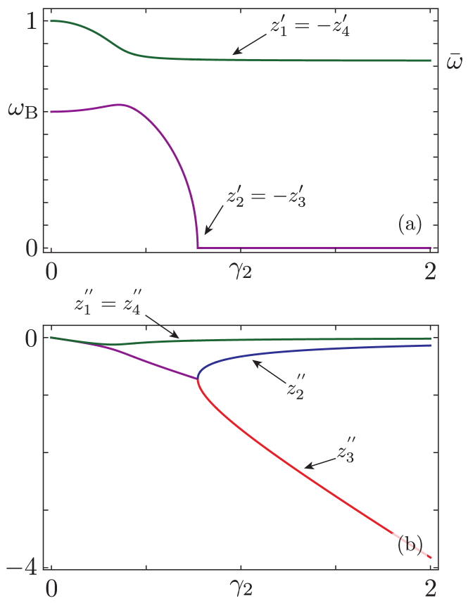
Figure 2: Plot of (a) the real part $z^{\prime}_{j}$ and (b) the imaginary part $z_{j}^{\prime\prime}$ of the four zeros of $D(\omega)$. These quantities are plotted as a function of the damping strength $\gamma_{2}(\omega)=\gamma_{2}$ for the representative parameter values $\omega_{A}=1$ and $\omega_{B}=0.6$. All quantities are in units of $\omega_{A}$.

In Fig. 2 we report the real – Panel (a) – and imaginary – Panel (b) – parts of the four zeros as a function of the damping strength $\gamma_{2}$. Looking at Fig. 2(a) it is easy to see that for $\gamma_{2}\ll\omega_{A,B}$ the system behaves as two independent QHOs with characteristic frequencies $\omega_{A}$ and $\omega_{B}$. On the other hand, at large damping $\gamma_{2}\geq\omega_{A,B}$ two modes are frequency locked to the common hybrid frequency $\bar{\omega}$ of Eq. (25), with $z_{1}^{\prime}=-z_{4}^{\prime}\to\bar{\omega}$, while the other two are overdamped, namely $z_{2}^{\prime}=-z_{3}^{\prime}=0$.

Considering now the imaginary parts in Fig. 2(b) we see that for small damping they all are $\propto\gamma_{2}$, and acquire different behaviours at larger $\gamma_{2}$. In particular the zeros that tend to a finite frequency $z_{1}^{\prime}=-z_{4}^{\prime}\to\bar{\omega}$, have imaginary parts that tend to vanish with increasing $\gamma_{2}$. On the other hand, the overdamped ones $z_{2}$ and $z_{3}$ possess imaginary contributions that run together until a critical value and bifurcate after it with opposite behaviour.

In the regime of very weak $\gamma_{2}\ll\omega_{A,B}$ or very strong damping $\gamma_{2}\gg\omega_{A,B}$ one can find analytical expressions for $z_{j}$. At very weak damping we obtain

$$z_{1,4}=\pm\omega_{A}-i\frac{\gamma_{2}}{2};\quad z_{2,3}=\pm\omega_{B}-i\frac{\gamma_{2}}{2},$$ (26)

while at ultra strong damping

$$\!\!z_{1,4}=\pm\bar{\omega}-i\frac{(\omega_{A}^{2}-\omega_{B}^{2})^{2}}{16\gamma_{2}\bar{\omega}^{2}};\,z_{2}=-i\frac{\omega_{A}^{2}\omega_{B}^{2}}{2\gamma_{2}\bar{\omega}^{2}};\,z_{3}=-2i\gamma_{2},$$ (27)

which fully agree with the behaviour reported in Fig. 2. Notice that the zeros that survive at the hybrid frequency $\bar{\omega}$ are very stable, i.e., with a very small imaginary part $\propto 1/\gamma_{2}$. This important behaviour is tightly related to the bath-mediated correlations. Indeed, $\gamma_{2}$ plays here a twofold role: it is responsible for dissipation but, at the same time, it also mediates an effective coupling between the two QHOs, instating non-trivial correlations between them even without any direct coupling a–priori. The above results demonstrate that at strong damping, the two QHOs become frequency locked oscillating, at finite time, with a common hybrid frequency $\bar{\omega}$. Moreover, they are also phase locked in anti–phase (relative phase fixed to $\pi$), as one can see from the relation of the homogeneous solution of Eq. (22) with $x_{A}(\omega)=-x_{B}(\omega)$ at large $\gamma_{2}$.

All these regimes are reflected on the retarded response function. Indeed, switching on the noise $\xi$, the system (22) has the long time compact solution ${\bf x}^{\dagger}={\bm{\chi}}_{2}\cdot{\bm{\xi}}^{\dagger}/m$, where ${\bf x}=(x^{(0)}_{A}(\omega),x^{(0)}_{B}(\omega))$ is the two-component vector of the oscillators, ${\bm{\xi}}=\xi_{2}(\omega)(1,1)$ is the noise vector and ${\bm{\chi}}_{2}(\omega)$ is the two-by-two response-function matrix, inverse of the coefficient matrix. Its elements are

$$\!\!\!\!\!\chi_{2}^{(ll)}(\omega)\!=\!\frac{-[\omega^{2}-\omega_{\bar{l}}^{2}+i\omega\gamma_{2}(\omega)]}{D(\omega)};\,\chi_{2}^{(l\bar{l})}(\omega)\!=\!\frac{i\omega\gamma_{2}(\omega)}{D(\omega)},$$ (28)

with $D(\omega)$ defined in Eq. (24). For completeness we also quote the imaginary parts, which enter into the expressions of the average power and heat currents (see Eqs. (18- III.1)):

$$\!\!\!{\chi_{2}^{(ll)}}^{\prime\prime}(\omega)=\frac{\omega(\omega^{2}-\omega_{{\bar{l}}}^{2})^{2}\gamma_{2}^{\prime}(\omega)}{|D(\omega)|^{2}},$$

$${\chi_{2}^{(l{\bar{l}})}}^{\prime\prime}(\omega)=\frac{\omega(\omega^{2}-\omega_{l}^{2})(\omega^{2}-\omega_{{\bar{l}}}^{2})\gamma_{2}^{\prime}(\omega)}{|D(\omega)|^{2}}~{}.$$ (29)

The behaviour of the response function is connected to the already discussed normal modes. More explicitly, at very weak damping ($\gamma_{2}\to 0$), ${\bm{\chi}}_{2}^{\prime\prime}(\omega)$ is exactly the one of two independent QHOs (see also Eq. (26)):

$${\chi_{2}^{(ll^{\prime})}}^{\prime\prime}(\omega)=\delta_{l,l^{\prime}}\frac{i\omega\gamma_{2}}{(\omega^{2}-\omega_{l}^{2})^{2}+\omega^{2}\gamma^{2}_{2}}.$$ (30)

In the opposite regime ($\gamma_{2}\to\infty$) from Eq. (27) we obtain

$${\chi_{2}^{(ll^{\prime})}}^{\prime\prime}(\omega)=\Big{[}(1-\delta_{l,l^{\prime}})+\frac{\omega_{\bar{l}}^{2}}{\omega_{l}^{2}}\delta_{l,l^{\prime}}\Big{]}\frac{\omega}{2\bar{\omega}^{2}}\frac{|z_{2}^{\prime\prime}|}{\omega^{2}+|z_{2}^{\prime\prime}|^{2}}$$

$$+(-1)^{1-\delta_{l,l^{\prime}}}\frac{\omega}{4\bar{\omega}^{2}}\sum_{p=\pm}\frac{|z_{1}^{\prime\prime}|}{(\omega+p\bar{\omega})^{2}+|z_{1}^{\prime\prime}|^{2}}\,.$$ (31)

Here, since $z_{1}^{\prime\prime}$ and $z_{2}^{\prime\prime}$ scale as $1/\gamma_{2}$ (see Eq. (27)), both the diagonal and the off diagonal response functions are dominated by contributions peaked around $\pm\bar{\omega}$. Indeed in this regime, the WM becomes effectively frequency locked to a unique characteristic frequency, i.e., $\bar{\omega}$. In addition, the phase locking at $\pi$, discussed above, is here reflected in the property ${\chi_{2}^{(l\bar{l})}}^{\prime\prime}(\omega)\to-{\chi_{2}^{(ll)}}^{\prime\prime}(\omega)$. Also, note that the first term in Eq. (31) $\propto\omega$ is negligible with respect to the second one, however it could give finite contributions to the power – although always dissipative, $P>0$, (see below).

We conclude this Section by quoting, for the sake of comparison, the behaviour associated to the independent configuration (see Fig. 1(b)). In this case the response funtion is diagonal and given by [49] $\chi_{2,\rm ind}^{(ll^{\prime})}(\omega)=-\delta_{l,l^{\prime}}/[\omega^{2}-\omega^{2}_{l}+i\omega\gamma_{2}]$. It is then straighforward to see that at very weak damping the normal modes are the same as in the joint case in Eq. (26), while for strong damping they are given by $z_{1,\rm ind}=-i\omega_{A}^{2}/\gamma_{2}$, $z_{2,\rm ind}=-i\omega_{B}^{2}/\gamma_{2}$ and $z_{3,4,\rm ind}=-i\gamma_{2}$. As we can see, in the latter case, all zeros are pure imaginary, implying always an overdamped regime at strong damping. This behaviour is in sharp contrast with the case discussed above of the joint configuration.

IV Quantum thermal machine performance

In this Section we present our main results concerning the effect of bath-mediated correlations on the performance of a quantum thermal machine operating as a dynamical heat engine. To evaluate power or heat currents, in addition to the response function ${\bm{\chi}}_{2}(\omega)$ discussed above, we also need to specify the spectral density ${\cal J}_{1}(\omega)$ of the dynamically, weakly coupled bath. As discussed in previous works [49, 50], memory effects and hence the precise shape of ${\cal J}_{1}(\omega)$ play an important role in determining the working regime. For this reason we choose a structured non-Markovian environment [61, 62, 63, 64, 65] with a Lorentzian spectral function

$${\cal J}_{1}(\omega)=\frac{d_{1}m\gamma_{1}\omega}{(\omega^{2}-{\omega}_{1}^{2})^{2}+\gamma_{1}^{2}\omega^{2}}~{},$$ (32)

with a peak centered at $\omega\sim{\omega}_{1}$, an amplitude governed by $d_{1}$, and a damping width determined by $\gamma_{1}$. Notice that for sufficiently small $\gamma_{1}$ this spectral density acts as an effective energy filter, centered around $\pm\omega_{1}$, for the working point of the thermal machine. Such structured environment represents a common example of non-Markovian bath that entails memory effect [64, 49] and can be realized with state-of-the-art superconducting circuits [66, 67, 68, 69]. Hereafter, we focus on the impact of bath-mediated correlations on the performance of dynamical heat engine. We will show the emergence of cooperative effects in the output power of the dynamical heat engine and how the strong dissipation regime can be a useful resource, when stable frequency locking has been established.

IV.1 Output power for monochromatic drivings

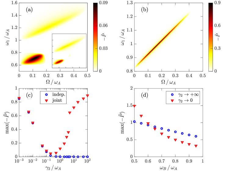
Figure 3: Output power of Eq. (34) for the dynamical heat engine with a monochromatic drive.(a) Density plot of the (dimensionless) output power $-\tilde{P}=-P\omega_{A}^{2}/d_{1}$ for the joint configuration as a function of $\Omega/\omega_{A}$ and $\omega_{1}/\omega_{A}$ with $\omega_{B}=0.6\omega_{A}$, $\phi=0$, and damping strength $\gamma_{2}=0.1\omega_{A}$. The inset shows the comparison with the independent configuration of Fig. 1(b), on the scame scale. (b) Same as in panel (a) but for strong dissipation with $\gamma_{2}=100\omega_{A}$ and $\phi=\pi$ (see text). (c) Maximum output power for the representative value $\omega_{B}=0.6\omega_{A}$ as a function of damping strength $\gamma_{2}$, both in the joint and in the independent case. (d) Maximum output power for the joint configuration in the very weak ($\gamma_{2}\to 0$) and ultra strong ($\gamma_{2}\to\infty$) regime, as a function of $\omega_{B}/\omega_{A}$. Other parameters are: $T_{1}=0.6\omega_{A}$, $T_{2}=0.4\omega_{A}$, and Lorentzian linewidth $\gamma_{1}=0.01\omega_{A}$.

We now investigate the output power produced by the heat engine, in the case of a monochromatic drive:

$$g_{1}^{(A)}(t)=\cos(\Omega t)~{},\quad g_{1}^{(B)}(t)=\cos(\Omega t+\phi)~{},$$ (33)

with $\Omega$ the external frequency and $\phi$ the phase displacement felt by the two QHOs composing the WM. Although the choice of a single harmonic might seem a simplifying assumption, we will show that in most cases this represents the optimal one (see Sec. IV.2). Inspecting Eq. (2) one has $g_{n}^{(A)}=\delta_{n,\pm 1}/2$ and $g_{n}^{(B)}=e^{\mp i\phi}\delta_{n,\pm 1}/2$ and Eq. (18) becomes

$$P=-\Omega\int_{-\infty}^{+\infty}\frac{{\rm d}\omega}{4\pi m}{\cal J}_{1}(\omega+\Omega)N(\omega,\Omega){\chi}_{{\rm eff}}^{\prime\prime}(\omega)~{},$$ (34)

with

$$\!\!\!\!\chi_{{\rm eff}}(\omega)={\chi_{2}^{(A,A)}}(\omega)+{\chi_{2}^{(B,B)}}(\omega)+2\cos(\phi){\chi_{2}^{(A,B)}}(\omega),$$ (35)

an effective response function that explicitly depends on the phase displacement $\phi$, which modulates the constructive/destructive interference induced by the non-diagonal term $\chi_{2}^{(A,B)}$. Looking for the optimal output power, it is easy to see that only two phase values are relevant, i.e., $\phi=0$ or $\phi=\pi$.

In order to see the effects of bath-mediated correlations, the output power produced by the joint configuration Fig. 1(a) should be compared to the one obtained in the independent configuration of Fig. 1(b). In the latter case $P$ is given by an expression analogous to Eq. (34) where $\chi_{{\rm eff}}(\omega)\to\chi_{{\rm eff,\rm ind}}(\omega)=-\sum_{l=A,B}(\omega^{2}-\omega_{l}^{2}+i\gamma_{2}\omega)^{-1}$.

In the limit of small damping strength $\gamma_{2}\to 0$, the response function ${\bm{\chi}}_{2}(\omega)$ reduces to the one of an independent configuration with two individual QHO in parallel (see Eq. (30)) and the bath cannot mediate any correlations. Therefore no cooperative effects are expected to show up in the $\gamma_{2}\to 0$ limit. However we know that the response functions qualitatively change while increasing the damping strength. To see these effects in Fig. 3(a) we start considering the case of a moderate damping strength $\gamma_{2}=0.1\omega_{A}$. Here, the engine output power is reported considering the temperature configuration [70] $T_{1}=0.6\omega_{A}$, $T_{2}=0.4\omega_{A}$, and the representative value $\omega_{B}=0.6\omega_{A}$. The density plot in the $\omega_{1}-\Omega$ plane shows the working regions of the dynamical heat engine, where $P<0$. From the figure it is clear that these regions follow two distinct sectors that correspond to the lines $\omega_{1}=\omega_{l}+\Omega$ with $l=A,B$. This is due to the Lorentzian spectral density of Eq. (32) that acts as an effective filter. In addition the two lines are clearly separate since the two oscillators are off resonance with $\omega_{B}=0.6\omega_{A}$. It is worth to note that the density plots in Fig. 3(a) have been obtained by optimizing with respect to the phase displacement $\phi$. For the representative value $\omega_{B}=0.6\omega_{A}$ the optimal output power is obtained for $\phi=0$. Already at this moderate damping $\gamma_{2}=0.1\omega_{A}$ a cooperative benefit in the output power starts to emerge, as one can see looking at the smaller values in the inset of Fig. 3(a). Here, the densitiy plot of the power for the independent case of Fig. 1(b) is reported for the same parameter values.

However, as demonstrated in the previous Section, the marked signature of bath-mediated correlations shows up in the strong dissipation regime ($\gamma_{2}\gg\omega_{A,B}$), when full frequency locking is established. The output power performance in this regime are reported in Fig. 3(b) with $\gamma_{2}=100\omega_{A}$. Strikingly, the joint configuration results in a wide and sizeable working regime for the dynamical heat engine. Moreover, differently from the density plot in Panel (a), the working region is now concentrated along a single line, i.e., $\omega_{1}\sim\bar{\omega}+\Omega$ that extends over a wider region in the $\omega_{1}-\Omega$ plane. The fact that only a single region now appears is consistent with the frequency locking mechanism, with the maximum power obtained in this case for $\phi=\pi$. In addition, comparing the moderate and strong damping situation, one can note a large increase in the output power magnitude observed for this parameter choice. The behaviour of the power as a function of the damping strength $\gamma_{2}$, both for the joint and the independent configuration, is analyzed in Fig. 3(c), where the maximum output power (obtained by maximizing over $\omega_{1}$, $\Omega$, and $\phi$) is reported. From this plot it is clear that above a certain critical value of $\gamma_{2}$ the independent configuration is fully overdamped and ceases to work as a heat engine, while on the contrary the joint configuration is not only stable but it can also perform better in the strong dissipation regime. Finally, in Fig. 3(d) we have reported the maximum output power of the joint case for the two opposite regimes of very weak ($\gamma_{2}\to 0$) and ultra strong ($\gamma_{2}\to\infty$) damping. These behaviours are obtained in an analytic form by replacing the results of $\chi_{2}^{(l,l^{\prime})}(\omega)$ into $\chi_{\rm eff}$ in Eq. (35) and then in Eq. (34). For $\gamma_{2}\to 0$, we use the diagonal form of $\chi_{2}^{(ll^{\prime})}(\omega)$ in Eq. (30) that gives a phase–independent, completely uncorrelated power

$$P=-\frac{\Omega}{8m}\sum_{l=A,B}\frac{1}{\omega_{l}}\sum_{p=\pm}p{\cal J}_{1}(p\omega_{l}+\Omega)N(p\omega_{l},\Omega).$$ (36)

In the opposite regime of $\gamma_{2}\to\infty$, we use the asymptotic expression of $\chi_{2}^{(ll^{\prime})}(\omega)$ given in Eq. (31). Here, the dependence on the phase $\phi$ is crucial in order to discriminate between constructive or destructive interference. For the constructive interference case ($\phi=\pi$) we have

$$\!\!P_{\pi}\!=\!\frac{\Omega}{4m\bar{\omega}}\!\Big{[}\frac{T_{2}(\omega_{B}^{2}-\omega_{A}^{2})^{2}}{\bar{\omega}\omega_{A}^{2}\omega_{B}^{2}}{\cal J}_{1}(\Omega)-\!\!\sum_{p=\pm}\!\!p{\cal J}_{1}(p\bar{\omega}+\Omega)N(p\bar{\omega},\Omega)\Big{]}.$$ (37)

For the destructive interference case, with $\phi=0$, the dominant contributions of $\chi_{2}^{(ll^{\prime})}(\omega)$, around the characteristic frequency $\bar{\omega}$, cancel out in $\chi_{\rm eff}$ and only the dissipative part around $\omega\to 0$ remains (see Eq. (31))

$$P_{0}=\frac{\Omega}{2m}T_{2}{\cal J}_{1}(\Omega)\left(\frac{1}{\omega_{A}^{2}}+\frac{1}{\omega_{B}^{2}}\right).$$ (38)

Here, one always has $P_{0}>0$ and no useful power can be delivered. Importantly, we notice that the corresponding power, $P_{\rm ind}$, of the independent configuration coincides exactly with the above result $P_{\rm ind}=P_{0}$. Indeed in this regime we have $\chi_{\rm eff}^{\rm ind}(\omega)=\sum_{l=A,B}i/\left[\gamma_{2}(\omega+i\omega_{l}^{2}/\gamma_{2})\right]$.

In Fig. 3(d), the maximum of $-P$ is inspected for different values of $\omega_{B}/\omega_{A}$ in the very weak and ultra-strong damping regimes (with $\phi=\pi$) reported in Eqs. (36) and (37). We clearly see that a wide region of parameters exists where the strong dissipation regime can outperform over its weak counterpart, demonstrating that frequency locking can be the optimal working point to benefit from cooperative effects.

IV.2 Pareto optimal performances

In Subsec. IV.1 we analyzed the power of the quantum thermal machine choosing for the driving controls $g_{1}^{(A)}(t)$ and $g_{1}^{(B)}(t)$, i.e., the single monochromatic shape given in Eq. (33). Here, we generalize the analysis of the cooperative effects on the performance of quantum thermal machine by (i) performing a functional optimization over arbitrary periodic driving functions $g_{1}^{(l)}(t)$, and (ii) deriving the Pareto front, i.e., the collection of driving functions that are Pareto-optimal tradeoffs between power and efficiency $\eta=-P/J_{1}$ [71]. We recall that a Pareto-optimal cycle is one such that it is not possible to further improve the power or efficiency, without sacrificing the other one. The Pareto-front is then defined as the collection of $(\eta,-P)$ points of all Pareto-optimal cycles, which in general will include the maximum power case, the maximum efficiency case, and intermediate tradeoffs. As shown in App. D, if a cycle is on the Pareto front of $(\eta,-P)$, it is also on the Pareto front of $(\sigma,-P)$, i.e., it is also a Pareto-optimal tradeoff between high power and low entropy production. Therefore, we search for the Pareto-front in $(\sigma,-P)$, and then transform these points to $(\eta,-P)$ removing the non-Pareto-optimal ones.

We determine the $(\sigma,-P)$ Pareto-front of the dynamical heat engine with respect to the driving coefficient $g_{n}^{(l)}$, i.e., with respect to all possible time-dependent periodic drivings $g_{1}^{(l)}(t)$, expressing both thermodynamic quantities as $-P(\{g_{n}^{(l)}\})$ and $\sigma(\{g_{n}^{(l)}\})$. As shown in App. D, without loss of generality we can assume the $g_{n}^{(l)}$ coefficients to be real. We then consider a collection of fixed values of the entropy production rate $\{\sigma_{i}\}$, and for each one, we repeat the following optimization problem

$$-P_{i}=\max_{\{g_{n}^{(l)}\}}{\left[-P(\{g_{n}^{(l)}\})\right]},$$ (39)

subject to:

$$\begin{aligned} \sigma(\{g_{n}^{(l)}\})&=\sigma_{i},\\ \sum_{n}|g_{n}^{(l)}|^{2}&=|g^{(l)}|^{2},\,\text{for }l=A,B,\end{aligned}$$

where $g^{(l)}$, for $l=A,B$, are two fixed constants. The Pareto front is then given by all points $\{(\sigma_{i},-P_{i})\}$. Using Parseval’s theorem, the last constraint in Eq. (39) is equivalent to bounding the time average of $|g_{1}^{(l)}(t)|^{2}$. This represents a normalization for the driving protocols motivated by the fact that all thermodynamic quantities scale as the square of the driving controls. Furthermore, it allows us to ensure that the coupling to bath 1 remains in the weak-coupling regime.

We solve the optimization problem in Eq. (39) numerically, using techniques commonly employed in the context of machine learning, considering a set of $5.000$ discrete frequencies, i.e., $10.000$ parameters $g_{n}^{(l)}$ with $n>0$ (negative frequency coefficients must be the same as positive ones to guarantee that $g^{(l)}(t)$ is real). We then use automatic differentiation and the ADAM algorithm [72], implemented in the PyTorch package [73], to perform a gradient descent optimization starting from a random guess of the driving parameters. A modification of the Lagrange multipliers technique suitable for a gradient descent approach [74] is used to enforce the entropy constraint in Eq. (39), while the last two constraints are exactly imposed renormalizing the coefficients (see App. E for details).

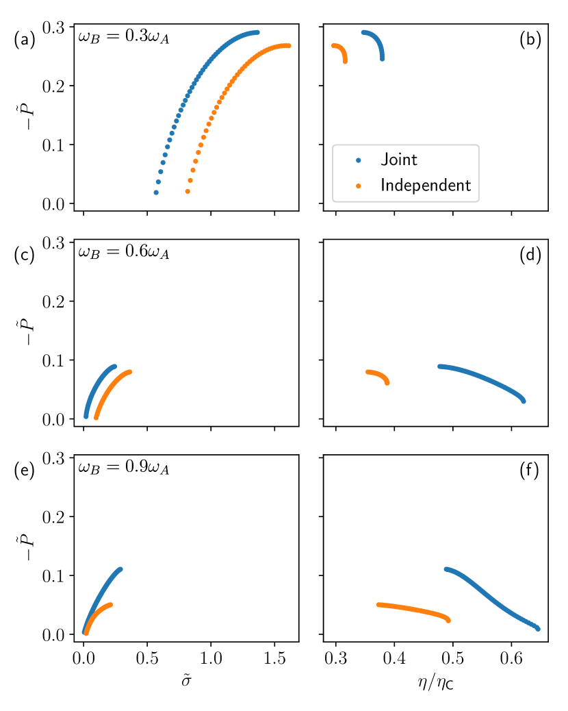
Figure 4: Comparison between the joint (blue dots) and independent (orange dots) Pareto front in the moderate damping case, i.e., $\gamma_{2}=0.1\omega_{A}$. The left column reports the Pareto front in the $(\tilde{\sigma},-\tilde{P})$ space, and the right column reports the same points in the $(\eta/\eta_{\text{C}},-\tilde{P})$, where $\eta_{\text{C}}=1-T_{2}/T_{1}$ is the Carnot efficiency. Each row corresponds to a different value of $\omega_{B}/\omega_{A}$: (a,b) correspond to $0.3$, (c,d) to $0.6$ and (e,f) to $0.9$. For each $\omega_{B}$, the value of $\omega_{1}$ is fixed to the one that yielded maximum power as in Fig. 3(a). The driving magnitudes are fixed to $|g^{(l)}|^{2}=0.5$, which are consistent with the monochromatic driving in Eq. (33). All other system parameters are chosen as in Fig. 3. The numerical calculations are performed optimizing over $5000$ evenly spaced frequencies, for each QHO, in the $[0,0.5\omega_{A}]$ interval. All plots report dimensionless quantities, i.e., $\tilde{P}=P\omega^{2}_{A}/d_{1}$ and $\tilde{\sigma}=\sigma/\omega_{A}$.

In Fig. 4 we report the results for the moderate damping case ($\gamma_{2}=0.1\omega_{A}$) studied in Fig. 3(a) for three representative values of $\omega_{B}$. In all cases, the value of $\omega_{1}$ has been chosen as the one that yielded the maximum output power.

The left and right columns correspond, respectively, to the Pareto front in the $(\sigma,-P)$ and $(\eta,-P)$ space. Each row corresponds to different values of $\omega_{B}/\omega_{A}=0.3,\ 0.6,\ 0.9$. Blue dots correspond to the joint case of Fig. 1(a), and orange dots to the independent configuration of Fig. 1(b).

Since we are interested in high power, low entropy production, and high efficiency, the performance of the engine improves as we move to the upper left corner in the left column of Fig. 4, and as we move to the upper right corner in the right column of Fig. 4. Notably, in all cases, the entire Pareto front of the bath-mediated situation in the joint case is strictly better than that of the independent configuration, i.e., for all points along the Pareto front of the independent case, there is at least one point in the joint case that yields higher power and higher efficiency. Furthermore, not only is the maximum power higher, but especially the efficiency of the cooperative case is enhanced along the entire Pareto front, reaching values that are twice as large in the $\omega_{B}/\omega_{A}=0.6,0.9$ cases [see panels (c-f) of Fig. 4]. Interestingly, as we move from $\omega_{B}=0.3\omega_{A}$ to $\omega_{B}=0.9\omega_{A}$, the Pareto fronts move from a region of high power and low efficiency [upper left corner in panels (b,d,f)] to a region of lower power but higher efficiency [lower right corner in panels (b,d,f)].

Again, the effect of the bath-mediated interaction between the QHOs is clearly visible, even in the moderate damping case, comparing the optimal driving in the joint and independent case. Indeed, in the latter, the optimal driving consists of applying two different frequencies to each QHO: intuitively, this is expected, since each QHO has itself a different characteristic frequency. However, in the joint case the optimal driving turns out to be monochromatic along the entire Pareto front, for all explored values of $\omega_{B}$ except for the $\omega_{B}=0.6\omega_{A}$ case, where two frequencies become optimal when the power is lower than $|\tilde{P}|\sim 0.086$. We report some examples of the distribution of driving coefficients in App. E.

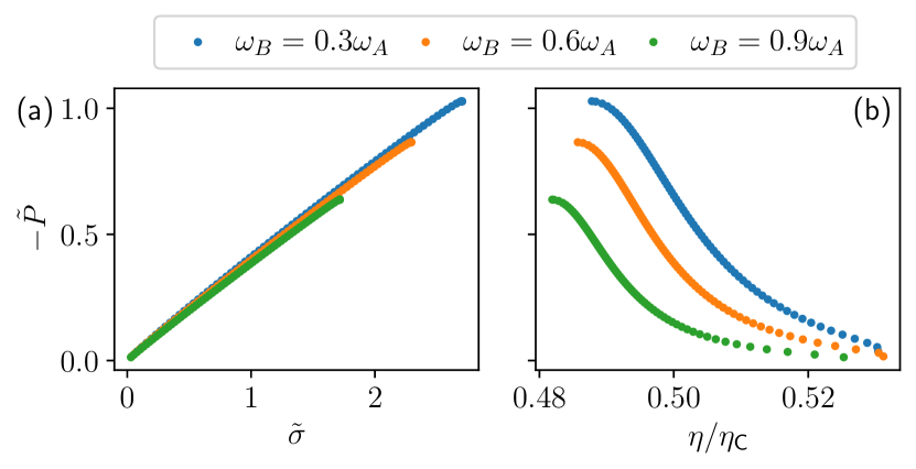
Figure 5: Pareto front of the joint case in the ultra-strong damping regime, i.e., $\gamma_{2}=100\omega_{A}$. As in Fig. 4, (a) reports the Pareto front in the $(\tilde{\sigma},-\tilde{P})$ space, and (b) reports the same points in the $(\eta/\eta_{\text{C}},-\tilde{P})$. Each curve corresponds to different values of $\omega_{B}/\omega_{A}$ as shown in the legend. The driving magnitudes are fixed to $|g^{(l)}|^{2}=0.5$, which are consistent with the monocromatic driving in Eq. (33). All other system parameters are chosen as in Fig. 3. The numerical calculations are performed optimizing over $5000$ evenly spaced frequencies, for each QHO, in the $[0,0.5\omega_{A}]$ interval.

In Fig. 5 we report the results for the strong dissipation regime at $\gamma_{2}/\omega_{A}=100$. As in Fig. 4, we fix $\omega_{1}$ to the value that yielded maximum power in the corresponding $\omega_{1}-\Omega$ plane and the left and right Panels corresponds, respectively, to the Pareto front in the $(\sigma,-P)$ and $(\eta,-P)$ space. The three curves correspond to the different values of $\omega_{B}$ reported in the legend.

Remarkably, the strong dissipation regime displays a high-performance Pareto front, reaching values of the power that are roughly three times larger than in the moderate damping regime, while operating at a high efficiency $\eta\sim 0.5\eta_{\text{C}}$. The optimal driving that emerges in the strong damping regime shares analogies with the moderate damping one in the joint configuration: in all cases analyzed in Fig. 5, the optimal driving along the entire Pareto front consists of a monochromatic drive (see also App. E).

IV.3 Measuring entanglement via average work

Before closing, we would like to emphasize another important result obtained in the strong damping regime: we will demonstrate that it is possible to find a direct prescription to assess the degree of entanglement in the joint case for the WM from measurements of average works. The quantifier we use for detecting quantum correlations is the so-called logarithmic negativity [55, 56, 36, 30] $E_{n}$ (see App. F for details). This quantity has been already inspected for gaussian states showing finite entanglement at steady state [31, 32, 34]. We remark that several recent studies [28, 29, 37, 34, 35] have investigated the potential role of quantum correlations in the performance of thermal machines, but a direct link between them is still an open issue. Here, we address a different aspect, i.e., a possible pathway to measure the degree of entanglement for a quantum system via thermodynamic observables.

We recall that the logarithmic negativity is defined as [55, 30]

$$E_{n}\equiv{\rm Max}\big{[}0,-\log(2\tilde{\nu})\big{]}~{},$$ (40)

where $\tilde{\nu}$ is the so-called symplectic eigenvalue of the partial transposed density matrix. in terms of position and momentum correlators, from which one can determine the value of the critical temperature. Strictly positive values of $E_{n}$ are a fingerprint of entanglement and therefore, to be in this regime, $\tilde{\nu}<1/2$ is required. This implies a constraint on temperatures: only for $T<T_{{\rm c}}$, with $T_{{\rm c}}$ a critical temperature, the WM will be entangled. The estimator $E_{n}$ is evaluated in App. F The behaviour of $T_{{\rm c}}$ is shown in Fig. 6 as a function of $\omega_{B}$ for different damping strengths $\gamma_{2}$. As one can see $T_{{\rm c}}$ tends to saturate to the valueremin $T^{*}$ which corresponds to the ultra-strong damping case $\gamma_{2}\to\infty$ (see below).

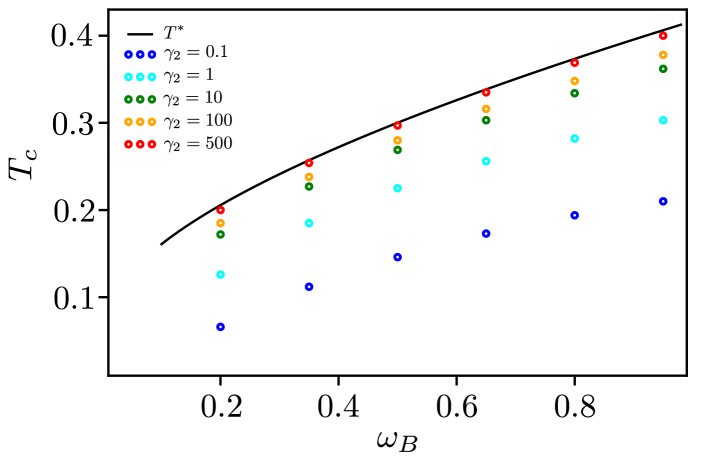
Figure 6: Behaviour of the critical temperature $T_{{\rm c}}$ below which non-zero entanglement in the WM is expected as a function of $\omega_{B}$. The black solid line represents the asymptotic behaviour at large $\gamma_{2}$, while different data points are for lower values of $\gamma_{2}$. Units of $\omega_{A}$.

Since $T^{*}$ is always the upper bound with respect to all other critical temperatures we decided to focus the following discussion at ultra-strong damping. Indeed this will be the best working point to enhance entanglement. In this regime we found (see App. F) a closed analytic expression for $\tilde{\nu}$ given by

$$\tilde{\nu}^{2}=\frac{\bar{\omega}^{4}\coth^{2}(y)}{4y\omega_{A}^{2}\omega_{B}^{2}}\frac{1}{\coth(y)+\frac{(\omega_{B}^{2}-\omega_{A}^{2})^{2}}{4y\omega_{A}^{2}\omega_{B}^{2}}};\,y=\frac{\bar{\omega}}{2T_{2}}~{}.$$ (41)

Using the above expression we obtain the critical temperature $T^{*}$ shown as black curve in Fig. 6.

Our task is now to demonstrate a direct link between $\tilde{\nu}$ in Eq. (41) and a function of works $W$ (directly obtained from the average power as $W=(2\pi/\Omega)P(\Omega)$) for differently driving protocols.

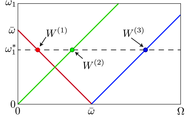
Figure 7: Sketch of the three working points in the $\omega_{1}-\Omega$ plane where we evaluate the average work $W^{(1,2,3)}$. The horizontal dotted line highlights the representative value for $\omega_{1}=\omega_{1}^{*}$ around which the spectral density ${\cal J}_{1}(\omega)$ is peaked.

As shown in the sketch of Fig. 7 we select three working points in the $\omega_{1}-\Omega$ plane which are obtained at the intersection between the horizontal dotted line at a fixed $\omega_{1}=\omega_{1}^{*}<\bar{\omega}$ and three lines: $\omega_{1}=\bar{\omega}-\Omega$ (red), $\omega_{1}=\Omega$ (green), $\omega_{1}=-\bar{\omega}+\Omega$ (blue). In addition we consider a peaked spectral function ${\cal J}_{1}(\omega)$, such that it acts as a sharp filter for frequencies that then need to be near to its maximum position $\omega_{1}^{*}$. Here, recalling the results of Sec.  IV.2 and thus focusing on the monochromatic drive, and using the power expressions in Eqs. (37)-(38) for the phases $\phi=\pi,0$ we obtain the work in the three points displayed in Fig. 7. For $\phi=\pi$ we have

$$W^{(1)}_{\phi=\pi}=-\frac{\pi}{2\bar{\omega}}{\cal J}_{1}(\omega_{1}^{*})N(-\bar{\omega},\bar{\omega}-\omega_{1}^{*})$$

$$W^{(2)}_{\phi=\pi}=\frac{\pi}{2}\frac{T_{2}}{\bar{\omega}^{2}}\frac{(\omega_{B}^{2}-\omega_{A}^{2})^{2}}{\omega_{A}^{2}\omega_{B}^{2}}{\cal J}_{1}(\omega_{1}^{*})$$

$$W^{(3)}_{\phi=\pi}=\frac{\pi}{2\bar{\omega}}{\cal J}_{1}(\omega_{1}^{*})N(-\bar{\omega},\bar{\omega}+\omega_{1}^{*})~{}.$$ (42)

On the other hand, at $\phi=0$, we obtain

$$W^{(2)}_{\phi=0}=\frac{\pi}{2}\frac{T_{2}}{\bar{\omega}^{2}}\frac{(\omega_{B}^{2}-\omega_{A}^{2})^{2}}{\omega_{A}^{2}\omega_{B}^{2}}{\cal J}_{1}(\omega_{1}^{*})$$ (43)

and $W^{(1)}_{\phi=0},W^{(3)}_{\phi=0}\to 0$. We now inspect the following combination of these average works: $\Delta W_{\phi}=W_{\phi}^{(2)}+W_{\phi}^{(3)}-W_{\phi}^{(1)}$. The result is

$$\Delta W_{\phi=\pi} = \frac{\pi}{\bar{\omega}}{\cal J}_{1}(\omega_{1})\left[\coth(y)+\frac{(\omega_{B}^{2}-\omega_{A}^{2})^{2}}{4y\omega_{A}^{2}\omega_{B}^{2}}\right]\,$$

$$\Delta W_{\phi=0} = \frac{\pi}{\bar{\omega}}{\cal J}_{1}(\omega_{1})\frac{\bar{\omega}^{4}}{y\omega_{A}^{2}\omega_{B}^{2}}.$$ (44)

Comparing these results with $\tilde{\nu}^{2}$ in Eq. (41) we arrive at the important identity

$$\tilde{\nu}^{2}=\frac{\coth^{2}\left(\frac{\bar{\omega}}{2T_{2}}\right)}{4}\frac{\Delta W_{\phi=0}}{\Delta W_{\phi=\pi}}.$$ (45)

This expression represents a direct link between entanglement and a function of the average works computed for specific driving protocols. To determine the value of entanglement via $\tilde{\nu}$ one can then use the following protocol: measure the average work in three different points and in the two opposite configurations $\phi=\pi$ and $\phi=0$. This link is universal and does not depend on the particular working regime of the thermal machine, provided that ultra-strong damping has been reached.

As a final remark, we recall that $\Delta W_{\phi=0}$ in Eq. (44) exactly corresponds to the same average work variation obtained in the independent configuration with separable QHOs (see discussion for the power in Sec.  IV.1 after Eq. (38))

$$\Delta W_{\phi=0}=\Delta W_{\rm ind}.$$ (46)

Therefore the equality (45) can be also rewritten in terms of work in the joint configuration $\Delta W_{\rm joint}=\Delta W_{\phi=\pi}$ and the independent one $\Delta W_{\rm ind}$. Interestingly this produces the following result: if the joint WM is in an entangled state ($4\tilde{\nu}^{2}<1$), then the corresponding work variation $\Delta W_{\rm joint}$ need always to fulfill the bound

$$\Delta W_{\rm joint}>\Delta W_{\rm ind}~{}.$$ (47)

V Conclusions

We have shown a cooperative advantage for a quantum heat engine made of two non-interacting quantum harmonic oscillators connected to common heat baths, with the couplings to one of them periodically driven. The cooperative advantage is rooted in the non-trivial correlations, mediated by the baths, established between the oscillators. Of particular interest is the regime of strong dissipation, where two independent single-oscillator engines working in parallel can not deliver any power, whereas with common baths the engine performance is comparable or even better than at weak dissipation. The fact that the strong dissipation is a a useful resource might seem surprising, but we have explained this result in terms of the appearance of a (weakly damped) frequency- and phase-locked mode, with the two oscillators moving with a common, hybrid frequency and oscillating in phase opposition. The claim of cooperative advantage has been corroborated by the optimization over generic periodic driving protocols, building the full Pareto fronts and thus providing the optimal tradeoffs between power and efficiency. As a final outcome of our work, we have found a precise prescription in terms of thermodynamic quantities, such as average works, able to assess the degree of entanglement present in the whole quantum system.

Our results open up several perspectives. First of all, it would be interesting to investigate whether the dissipation-induced cooperative advantage can be extended to $N>2$ oscillators and possibly establish a link, if any, between cooperative advantage and multipartite quantum correlations. Secondly, it would be interesting to consider different, non linear working media, in particular hybrid oscillator-qubit systems of particular interest for quantum computing and more generally for quantum technologies. Thirdly, our Pareto-front analysis paves the way to the use of machine learning tools for non-Markovian quantum thermodynamics processes. For the same model discussed here, it would be interesting to compute the Pareto-optimal front for the three desiderata of a heat engine (efficiency close to the Carnot efficiency, high output power, and constancy of the power output), investigating whether in some configuration it would be possible to go beyond the limits set by thermodynamic uncertainty relations [75, 76, 77, 78, 79] on the simultaneous achievement of such quantities.

Appendix A The counter-term of a dissipative two oscillators system

In this Section we derive the counter-term that appears in the interaction Hamiltonian $H^{(t)}_{{\rm int},\nu}$, (Eq. (6)) in the presence of two baths $\nu=1,2$. The $\nu$-th bath is of Caldeira–Leggett type [45], with free Hamiltonian

$$H_{\nu}=\sum_{k=1}^{+\infty}\left[\frac{P_{k,\nu}^{2}}{2m_{k,\nu}}+\frac{1}{2}m_{k,\nu}\omega_{k,\nu}^{2}X_{k,\nu}^{2}\right]~{}.$$ (48)

The coupling between the WM and the $\nu$-bath is of the form

$$H^{(t)}_{{\rm int},\nu}=-\Big{[}\sum_{l=A,B}\sum_{k=1}^{+\infty}g_{\nu}^{(l)}(t)c_{k,\nu}^{(l)}x_{l}X_{k,\nu}\Big{]}+H_{{\rm c.t.},\nu}.$$ (49)

Here, the last term $H_{{\rm c.t.},\nu}$ represents the so-called counter-term contribution that prevents possible renormalizations of the QHOs potentials $V_{l}(x_{l})=\frac{1}{2}m\omega_{l}^{2}x_{l}^{2}$ with $l=A,B$. Indeed, it is well known that the first term of $H^{(t)}_{{\rm int},\nu}$ introduces a renormalization of the frequencies $\omega_{l}$ and induces a direct coupling between the QHOs [80]. The counter-term is then inserted in order to avoid these effects. Since the couplings between the two oscillators, $x_{A}$ and $x_{B}$, and the bath coordinates $X_{k,\nu}$ are linear, the general form of $H_{{\rm c.t.},\nu}$ will be

$$H_{{\rm c.t.},\nu}=\lambda_{\nu}^{(A)}x_{A}^{2}+\lambda_{\nu}^{(AB)}x_{A}x_{B}+\lambda_{\nu}^{(B)}x_{B}\,,$$ (50)

where the three coefficients (for each bath $\nu$) are now determined with the following standard procedure [46, 80]. We consider the minimum of the total Hamiltonian $H^{(t)}$ (see Eq. (3)) with respect to the environment and the WM coordinates. From the requirement $\frac{\partial H^{(t)}}{\partial X_{k,\nu}}=0$ we obtain

$$X_{k,\nu}=\sum_{l=A,B}\frac{g_{\nu}^{(l)}(t)c_{k,\nu}}{m_{k,\nu}\omega_{k,\nu}^{2}}x_{l}\,.$$ (51)

This value will be used to determine the minimum of the Hamiltonian with respect to the WM coordinates $x_{l}$, which is given by

$$\frac{\partial H^{(t)}}{\partial x_{l}}=\frac{\partial V_{l}(x_{l})}{\partial x_{l}}+\frac{\partial H_{{\rm c.t.},\nu}}{\partial x_{l}}-\!\!\sum_{l=A,B}\sum_{k=1}^{+\infty}g_{\nu}^{(l)}(t)c_{k,\nu}^{(l)}X_{k,\nu}.$$ (52)

Now, to avoid renormalization effects we impose that this minimum corresponds to the minimum of the bare potential $V_{l}(x_{l})$

$$\frac{\partial H^{(t)}}{\partial x_{l}}=\frac{\partial V_{l}(x_{l})}{\partial x_{l}}\qquad\text{for }l=A,B\,.$$ (53)

This constraint results in the following relations

$$\sum_{k=1}^{+\infty}g_{\nu}^{(l)}(t)c_{k,\nu}^{(l)}X_{k,\nu}=2\lambda_{\nu}^{(l)}x_{l}+\lambda_{\nu}^{(AB)}x_{\bar{l}},$$ (54)

where we remind the convention according to which if $l=A$ then $\bar{l}=B$, and vice versa. Inserting now Eq. (51) into (54) we get

$$\lambda_{\nu}^{(A)}=\sum_{k=1}^{+\infty}\frac{(g_{\nu}^{(A)}(t)c_{k,\nu}^{(A)})^{2}}{2m_{k,\nu}\omega_{k,\nu}^{2}};\,\lambda_{\nu}^{(B)}=\sum_{k=1}^{+\infty}\frac{(g_{\nu}^{(B)}(t)c_{k,\nu}^{(B)})^{2}}{2m_{k,\nu}\omega_{k,\nu}^{2}}$$

$$\lambda_{\nu}^{(AB)}=\sum_{k=1}^{+\infty}\frac{g_{\nu}^{(A)}(t)g_{\nu}^{(B)}(t)c_{k,\nu}^{(A)}c_{k,\nu}^{(B)}}{m_{k,\nu}\omega_{k,\nu}^{2}}.$$ (55)

The final form of $H^{(t)}_{{\rm int},\nu}$, quoted in the main text (see Eq. (6), is now obtained from the interaction form in Eq. (49), with the counter-term given in Eqs. (50) and (55). Notice that in this Appendix, for completeness, we left the explicit indices $A$ and $B$ in $c_{k,\nu}^{(A)}$ and $c_{k,\nu}^{(B)}$. In the following we will consider always $c_{k,\nu}^{(A)}=c_{k,\nu}^{(B)}$.

Appendix B Time dependence evolutions of WM and baths coordinates

Starting from Eq. (3) the equations of motion, in the Heisenberg picture, for the QHO’s and reservoir degrees of freedom are, respectively,

$$\begin{cases}\dot{x}_{l}\!\!\!\!&=\dfrac{p_{l}}{m}\,,\\ \dot{p}_{l}\!\!\!\!&=-m\omega_{l}^{2}x_{l}-{\displaystyle\sum_{\nu=1,2}}{\displaystyle\sum_{k=1}^{+\infty}}\bigg{[}-g_{\nu}^{(l)}(t)c_{k,\nu}X_{k,\nu}\\ \!\!\!\!&+\dfrac{(g_{\nu}^{(l)}(t)c_{k,\nu})^{2}}{m_{k,\nu}\omega_{k,\nu}^{2}}x_{l}+\dfrac{g_{\nu}^{(l)}(t)g_{\nu}^{(\bar{l})}(t)c_{k,\nu}^{2}}{m_{k,\nu}\omega_{k,\nu}^{2}}x_{\bar{l}}\bigg{]}\,,\end{cases}$$ (56)

and

$$\begin{cases}\dot{X}_{k,\nu}\!\!\!\!&=\dfrac{P_{k,\nu}}{m_{k,\nu}}\,,\\ \dot{P}_{k,\nu}\!\!\!\!&=-m_{k,\nu}\omega_{k,\nu}^{2}X_{k,\nu}+{\displaystyle\sum_{l=A,B}}g_{\nu}^{(l)}(t)c_{k,\nu}x_{l}\,,\end{cases}$$ (57)

where the overdots denote time derivatives. The solution for the position operator of the $k$-th oscillator of the $\nu$th reservoir is exact and can be written in terms of the WM coordinates

$$X_{k,\nu}(t) =\xi_{k,\nu}(t)+\sum_{l=A,B}\frac{c_{k,\nu}}{m_{k,\nu}\omega_{k,\nu}}\int_{t_{0}}^{t}{\rm d}s\,g_{\nu}^{(l)}(s)x_{l}(s)$$

$$\quad\times\sin[\omega_{k,\nu}(t-s)],$$ (58)

where we have introduced

$$\xi_{k,\nu}(t)\equiv X_{k,\nu}(t_{0})\cos[\omega_{k,\nu}(t-t_{0})]$$

$$+\frac{P_{k,\nu}(t_{0})}{m_{k,\nu}\omega_{k,\nu}}\sin[\omega_{k,\nu}(t-t_{0})],$$ (59)

and $t_{0}\to-\infty$ the initial time. Notice that the corresponding fluctuating noise is

$$\xi_{\nu}(t)=\sum_{k=1}^{+\infty}c_{k,\nu}\xi_{k,\nu}(t),$$ (60)

with zero quantum average $\langle\xi_{\nu}(t)\rangle=0$ and correlator written in Eq. (II.2).

To determine the time behaviour of $x_{l}(t)$ we remind that we have assumed the coupling to the reservoir $\nu=1$ much weaker with respect to the one with $\nu=2$. In this spirit, we will treat the interaction term $H^{(t)}_{\rm int,\nu=1}$ in Eq. (6) perturbatively. We can then split the total Hamiltonian $H^{(t)}$ in Eq. (3) as $H^{(t)}=H^{(0)}+H^{(t)}_{\rm int,\nu=1}$, where $H^{(0)}$ is the ”unperturbed” part, which contains all the contributions of $H^{(t)}$ apart $H^{(t)}_{\rm int,\nu=1}$ which is indeed the perturbation. Within this procedure the time dependence of the position operator of the $l$-th QHO is

$$x_{l}(t)=x_{l}^{(0)}(t)+\Delta x_{l}(t).$$ (61)

Here, the first term is the leading one and it evolves under the influence of the static $\nu=2$ reservoir

$$x_{l}^{(0)}(t)=e^{iH^{(0)}(t-t_{0})}x_{l}^{(0)}e^{-iH^{(0)}(t-t_{0})}~{}.$$ (62)

On the other hand, the second term is the perturbative correction evaluated at lowest order in $H^{(t)}_{\rm int,\nu=1}$

$$\Delta x_{l}(t) =-i\int_{t_{0}}^{t}{\rm d}s\sum_{l^{\prime}=A,B}g_{1}^{(l^{\prime})}(s)\xi_{1}(s)\big{[}x_{l^{\prime}}^{(0)}(s),x_{l}^{(0)}(t)\big{]}~{}.$$ (63)

From the above expressions it is clear that the time dependence of $x_{A,B}(t)$ is directly obtained from the time behaviour of the leading terms ${x}^{(0)}_{A,B}(t)$. These latter operators obey the coupled Langevin equations in the presence of the coupling with the static bath $\nu=2$. We have ($l=A,B$; $\bar{l}=B,A$)

$$\ddot{x}^{(0)}_{l}(t) +\omega_{l}^{2}x^{(0)}_{l}(t)+\int_{-\infty}^{t}{\rm d}s~{}\Big{[}\gamma_{2}(t-s)\dot{x}^{(0)}_{l}(s)$$

$$+\gamma_{2}(t-s)\dot{x}^{(0)}_{\bar{l}}(s)\Big{]}=\frac{\xi_{2}(t)}{m}\,,$$ (64)

with damping kernel

$$\gamma_{\nu}(t)=\frac{1}{m}\sum_{k=1}^{+\infty}\frac{c_{k,\nu}^{2}}{m_{k,\nu}\omega_{k,\nu}^{2}}\cos(\omega_{k,\nu}t)~{},$$ (65)

and noise $\xi_{2}(t)$ given in Eq. (60). The formal solution, in the long time limit, can be written as a convolution

$$x^{(0)}_{l}(t)=\sum_{l^{\prime}=A,B}\frac{1}{m}\int_{-\infty}^{+\infty}{\rm d}s\chi_{2}^{(l,l^{\prime})}(t-s)\xi_{2}(s)~{},$$ (66)

where we have introduced the retarded response function (see also Sec. III)

$$\chi^{(ll^{\prime})}_{2}(t)\equiv im\theta(t)\langle[x^{(0)}_{l}(t),x_{l^{\prime}}^{(0)}(0)]\rangle~{}.$$ (67)

Notice that here the quantum averages $\langle\dots\rangle$ are performed only with respect to the static $\nu=2$ reservoir contribution and can be taken as thermal averages since we are interested in the long time behaviour.

Appendix C Perturbative expressions of thermodynamic quantities

In this Section we derive closed expressions for the average power and heat currents under the assumption that the (time-dependent) couplings with the $\nu=1$ reservoir are weak. We start by considering the power expression in Eq. (II.2). Inserting the solution $X_{k,1}(t)$ of Eq. (58), and after an integration by parts (exploiting also that $g_{1}(t_{0})=0$ because the coupling is switched on at $t_{0}^{+}$), we obtain

$${P}(t)=-\sum_{l=A,B}\dot{g}_{1}^{(l)}(t)x_{l}(t)\bigg{\{}\xi_{1}(t)$$

$$-\sum_{l^{\prime}=A,B}m\int_{t_{0}}^{t}{\rm d}s\,\gamma_{1}(t-s)\frac{{\rm d}}{{\rm d}s}[g_{1}^{(l^{\prime})}(s)x_{l^{\prime}}(s)]\bigg{\}}\,,$$ (68)

with the damping function defined in Eq. (65). Now, using Eq. (61), we write $P(t)$ at the lowest perturbative order

$${P}(t)=-\!\!\sum_{l=A,B}\bigg{\{}\!\dot{g}_{1}^{(l)}(t)[x_{l}^{(0)}(t)+\Delta x_{l}(t)]\xi_{1}(t)$$

$$-\!\dot{g}_{1}^{(l)}(t)x_{l}^{(0)}(t)\!\!\!\!\sum_{l^{\prime}=A,B}m\int_{t_{0}}^{t}\!\!\!{\rm d}s\,\gamma_{1}(t-s)\frac{{\rm d}}{{\rm d}s}[g_{1}^{(l^{\prime})}(s)x_{l^{\prime}}^{(0)}(s)]\!\bigg{\}}.$$ (69)

In order to perform the quantum average $\langle P(t)\rangle$ we first notice that $\langle x_{l}^{(0)}(t)\dot{\xi}_{1}(t^{\prime})\rangle=0$, since at this perturbative order $x_{l}^{(0)}(t)$ and $\dot{\xi}_{1}(t)$ are completely decoupled. In addition, it is useful to introduce in Eq. (68) the WM correlators

$$C^{(l,l^{\prime})}(t,s)\equiv C^{(l,l^{\prime})}(t-s)=\langle x_{l}^{(0)}(t)x_{l^{\prime}}^{(0)}(s)\rangle~{},$$ (70)

with combinations

$$C_{\pm}^{(l,l^{\prime})}(\tau)=C^{(l,l^{\prime})}(\tau)\pm C^{(l^{\prime},l)}(-\tau)~{},$$ (71)

and to change variable $\tau=t-s$. After these steps it is then straighforward to perform the average $\langle P(t)\rangle$ also over the period. Defining the function

$$G^{(l,l^{\prime})}(\tau)=\int_{{0}}^{{\cal T}}\frac{{\rm d}t}{{\cal T}}\dot{g}_{1}^{(l)}(t)g_{1}^{(l^{\prime})}(t-\tau)\,,$$ (72)

we arrive at

$$P= -i\!\sum_{l,l^{\prime}=A,B}\int_{0}^{+\infty}\!\!\!\!\!{\rm d}\tau\,G^{(l,l^{\prime})}(\tau)\Big{\{}{\cal L}_{1,{\rm s}}(\tau)C_{-}^{(l,l^{\prime})}(\tau)$$ (73)

$$+{\cal L}_{1,{\rm a}}C_{+}^{(l,l^{\prime})}(\tau)\Big{\}}~{}.$$

In the above expression, we have ${\cal L}_{1}(\tau)\equiv{\cal L}_{1,{\rm s}}(\tau)+{\cal L}_{1,{\rm a}}(\tau)$ with symmetric and anti-symmetric parts

$${\cal L}_{1,{\rm s}}(t) = \int_{0}^{+\infty}\!\!\frac{{\rm d}\omega}{\pi}{\cal J}_{1}(\omega)\coth(\frac{\omega}{2T_{1}})\cos(\omega t),$$

$${\cal L}_{1,{\rm a}}(t) = -i\int_{0}^{+\infty}\!\!\frac{\mathrm{d}\omega}{\pi}{\cal J}_{1}(\omega)\sin(\omega t)~{}.$$ (74)

Notice that ${\cal L}_{1}(\tau)$ corresponds to the noise correlator $\langle\xi_{1}(\tau)\xi_{1}(0)\rangle$ defined in Eq. (II.2) and depends on the bath spectral density ${\cal J}_{1}(\omega)$. For the sake of completeness we quote also the identity $m\dot{\gamma}_{1}(t)=-2i{\cal L}_{1,{\rm a}}(t)$. To obtain now the final expression for the power we use the Fourier components of the functions ${\cal L}_{1,{\rm{s,a}}}(\tau)$ and $C_{\pm}^{(l,l^{\prime})}(\tau)$. They are

$${\cal L}_{1,{\rm s}}(\omega) = {\cal J}_{1}(\omega)\coth\left(\frac{\omega}{2T_{1}}\right);\quad{\cal L}_{1,{\rm a}}(\omega)={\cal J}_{1}(\omega)$$

$$C_{+}^{(l,l^{\prime})}(\omega) = \frac{2}{m}\coth\left(\frac{\omega}{2T_{2}}\right){\chi_{2}^{(l,l^{\prime})}}^{\prime\prime}(\omega)~{},$$

$$C_{-}^{(l,l^{\prime})}(\omega) = \frac{2}{m}{\chi_{2}^{(l,l^{\prime})}}^{\prime\prime}(\omega)~{}.$$ (75)

For $C_{\pm}^{(l,l^{\prime})}(\omega)$ we used the fluctuation dissipation relation that links these correlators to the imaginary part of the response function $\chi_{2}^{(l,l^{\prime})}(\omega)$. Concerning $G^{(l,l^{\prime})}(\tau)$ in Eq. (72) we use the decomposition (see Eq. (2))

$$G^{(l,l^{\prime})}(\tau)=-i\sum_{n=-\infty}^{+\infty}n\Omega g_{n}^{(l)}g_{-n}^{(l^{\prime})}e^{-in\Omega\tau}~{}.$$ (76)

Exploiting these Fourier representations in Eq. (73), one eventually arrives at the final expression for the average power

$$P\!=\!-\!\!\!\!\sum_{n=-\infty}^{+\infty}\!\!\!n\Omega\!\!\int_{-\infty}^{+\infty}\!\!\!\frac{{\rm d}\omega}{2\pi m}{\cal J}_{1}(\omega+n\Omega)N(\omega,n\Omega){\bf g}^{\dagger}_{n}\cdot{\bm{\chi}}_{2}^{\prime\prime}(\omega)\cdot{\bf g}_{n}\,,$$ (77)

where ${\bf g}_{n}=(g_{n}^{(A)},g_{n}^{(B)})$ is a two-element vector and ${\bf g}_{n}^{\dagger}$ its adjoint. We have also used the compact matrix notation ${\bm{\chi}}_{2}^{\prime\prime}(\omega)$, which is a two-by-two matrix whose entries are the imaginary parts of the response functions ${\chi_{2}^{(l,l^{\prime})}}(\omega)$ taken from Eq. (67), and introduced

$$N(\omega,\Omega)=\coth\left(\frac{\omega+\Omega}{2T_{1}}\right)-\coth\left(\frac{\omega}{2T_{2}}\right)\,.$$ (78)

Concerning the average heat currents $J_{\nu}$, similar steps as detailed above can be followed. Here, we briefly report few of them to arrive to the final closed expressions. Considering Eq. (11) and expanding $x_{l}(t)$ as in Eq. (61), we have

$$J_{1}(t)=-\!\!\sum_{l=A,B}g_{1}^{(l)}(t)\biggl{[}x_{l}^{(0)}(t)\dot{\xi}_{1}^{(l)}(t)+\Delta x_{l}(t)\dot{\xi}_{1}^{(l)}(t)$$

$$-m\!\!\sum_{l^{\prime}=A,B}\int_{t_{0}}^{t}{\rm d}s\,x_{l}^{(0)}(t)x_{l^{\prime}}^{(0)}(s)g_{1}^{(l^{\prime})}(s)\ddot{\gamma}_{1}(t-s)\biggr{]}.$$ (79)

After taking the quantum average, the lowest order perturbative expression reads

$$\langle J_{1}(t)\rangle=\sum_{l,l^{\prime}=A,B}\int_{t_{0}}^{t}{\rm d}s\,g_{1}^{(l)}(t)g_{1}^{(l^{\prime})}(s)\biggl{\{}m\ddot{\gamma}_{1}(t-s)$$

$$\times C^{(l,l^{\prime})}(t-s)-i\langle\xi_{1}(s)\dot{\xi}_{1}(t)\rangle C_{-}^{(l,l^{\prime})}(t-s)\biggr{\}}~{}.$$ (80)

As before, the average over one period of the drive is performed by introducing the correlators in Eq. (71), exploiting the Fourier decomposition in Eq. (2) and using Eqs. (72)-(76). After some straightforward steps one arrives at

$$J_{1}\!=\!\sum_{n=-\infty}^{+\infty}\int_{-\infty}^{+\infty} \frac{{\rm d}\omega}{2\pi m}(\omega+n\Omega){\cal J}_{1}(\omega+n\Omega)N(\omega,n\Omega)$$

$$\times{\bf g}^{\dagger}_{n}\cdot{\bm{\chi}}^{\prime\prime}_{2}(\omega)\cdot{\bf g}_{n}~{},$$ (81)

and similarly for the other heat current

$$J_{2}\!=\!-\!\!\!\!\sum_{n=-\infty}^{+\infty}\!\int_{-\infty}^{+\infty}\!\!\!\frac{{\rm d}\omega}{2\pi m}\omega{\cal J}_{1}(\omega+n\Omega)N(\omega,n\Omega){\bf g}^{\dagger}_{n}\cdot{\bm{\chi}}^{\prime\prime}_{2}(\omega)\cdot{\bf g}_{n}~{}.$$ (82)

Appendix D General properties of the Pareto front

In this appendix we derive general properties of the Pareto-front and of the corresponding optimal driving. In particular, we prove that: (i) Pareto optimal drives for $(\eta,-P)$ are also optimal for $(\sigma,-P)$; (ii) the $(\sigma,-P)$ Pareto front is weakly convex; (iii) the strictly convex (linear) part of the Pareto front can be described by real coefficients $g_{n}^{(l)}$ involving at most two (four) frequencies, i.e., they are zero except for two (four) values of $n$; (iv) the time-average of Pareto optimal drives is zero, i.e., $g_{0}^{(l)}=0$.

Since the time-dependent controls $g_{1}^{(l)}(t)$ are real, their Fourier coefficients satisfy the property $g_{-n}^{(l)}=(g_{n}^{(l)})^{*}$. Using this, and the fact that $\chi_{2}^{(AB)}(\omega)=\chi_{2}^{(BA)}(\omega)$, we can rewrite the power and entropy production rate, starting from Eqs. (18) and (III.1), as

$$P(\{{\bf g}_{n}\}) =\sum_{n=1}^{+\infty}{\bf g}_{n}^{\dagger}\cdot I_{n}^{(P)}\cdot{\bf g}_{n},$$ (83)

$$\sigma(\{{\bf g}_{n}\}) =\sigma_{0}+\sum_{n=1}^{+\infty}{\bf g}_{n}^{\dagger}\cdot I_{n}^{(\sigma)}\cdot{\bf g}_{n},$$ (84)

where the sums extend only over positive frequencies and $I_{n}^{(P)}$ and $I_{n}^{(\sigma)}$ are 2x2 real and symmetric matrices given by

$$\left[I^{(P)}_{n}\right]_{ll^{\prime}}=-(n\Omega)\,\int_{-\infty}^{+\infty}\frac{{\rm d}\omega}{2\pi m}\Big{[}\mathcal{J}_{1}(\omega+n\Omega)N(\omega,n\Omega)\\ -\mathcal{J}_{1}(\omega-n\Omega)N(\omega,-n\Omega)\Big{]}{\chi_{2}^{(ll^{\prime})}}^{\prime\prime}(\omega),$$ (85)

$$\left[I^{(\sigma)}_{n}\right]_{ll^{\prime}}=-\frac{1}{T_{1}}\left[I^{(P)}_{n}\right]_{ll^{\prime}}+\left(\frac{1}{T_{2}}-\frac{1}{T_{1}}\right)\int_{-\infty}^{+\infty}\frac{{\rm d}\omega}{2\pi m}\,\omega\\ \times\Big{[}\mathcal{J}_{1}(\omega+n\Omega)N(\omega,n\Omega)+\mathcal{J}_{1}(\omega-n\Omega)N(\omega,-n\Omega)\Big{]}\\ \times{\chi_{2}^{(ll^{\prime})}}^{\prime\prime}(\omega),$$ (86)

for $l,l^{\prime}=\{A,B\}$. In Eq. (84) $\sigma_{0}=(1/2){\bf g}_{0}^{\dagger}\cdot I_{0}^{(\sigma)}\cdot{\bf g}_{0}$ is the entropy production rate given by the zero-frequency driving, i.e., the entropy production rate when the coupling is constant in time. The second law of thermodynamics prescribes $\sigma_{0}\geq 0$. Since the zero frequency component ${\bf g}_{0}$ does not contribute to the power and it only has a detrimental effect on the entropy production rate, all Pareto-optimal drivings will have ${\bf g}_{0}=0$. From now on we thus set ${\bf g}_{0}=0$.

We now define the $2N_{\text{max}}$-component vector

$${\bf g}=\begin{pmatrix}g_{1}^{(A)},&g_{1}^{(B)},&g_{2}^{(A)},&g_{2}^{(B)},&\dots,&g_{N_{\text{max}}}^{(A)},&g_{N_{\text{max}}}^{(B)}\end{pmatrix}^{t},$$ (87)

where $N_{\text{max}}$ is a maximum cut-off value (not to be confused with $\omega_{c}$) introduced for numerical purposes. With this definition, ${\bf g}$ is given by the concatenation of ${\bf g}_{n}$ for all $n=1,2,\dots,N_{\text{max}}$. Let us further introduce two $(2N_{\text{max}})$x$(2N_{\text{max}})$ matrices, $I^{(P)}$ and $I^{(\sigma)}$, such that Eqs. (83) and (84) can be written as

$$P({\bf g}) ={\bf g}^{\dagger}\cdot I^{(P)}\cdot{\bf g}, \sigma({\bf g}) ={\bf g}^{\dagger}\cdot I^{(\sigma)}\cdot{\bf g}.$$ (88)

Importantly, $I^{(P)}$ and $I^{(\sigma)}$ are block-diagonal matrices with 2x2 blocks along the diagonal given by, respectively, $I^{(P)}_{1}$, $I^{(P)}_{2}$, …$I^{(P)}_{N_{\text{max}}}$ and $I^{(\sigma)}_{1}$, $I^{(\sigma)}_{2}$, …$I^{(\sigma)}_{N_{\text{max}}}$. Therefore, they have the property that they only mix components with the same frequency index $n$.

Our goal is to characterize the $(\sigma,-P)$ and the $(\eta,-P)$ Pareto fronts assuming that $I^{(P)}$ and $I^{(\sigma)}$ are fixed matrices. The optimization is performed with respect to the vector ${\bf g}$ with $2N_{\text{max}}$ components. We assume that $\Omega$ is a sufficiently small frequency such that $n\Omega$ is approximately continuous. We then consider a large value of $N_{\text{max}}$ such that $N_{\text{max}}\Omega=0.5\omega_{A}$. This corresponds to optimizing the performance of the quantum thermal machine with respect to an arbitrary driving. The optimization is carried out imposing the two constraints on the Fourier coefficients given in Eq. (39). These constraints can be conveniently written in terms of $\bf{g}_{n}$ as

$$\sum_{n=1}^{+\infty}{\bf g}_{n}^{\dagger}\cdot\Pi^{(A)}_{n}\cdot{\bf g}_{n} =|g^{(A)}|^{2}, \sum_{n=1}^{+\infty}{\bf g}_{n}^{\dagger}\cdot\Pi^{(B)}_{n}\cdot{\bf g}_{n} =|g^{(B)}|^{2},$$ (89)

where

$$\Pi^{(A)}_{n} =\begin{pmatrix}1&0\\ 0&0\end{pmatrix}, \Pi^{(B)}_{n} =\begin{pmatrix}0&0\\ 0&1\end{pmatrix},$$ (90)

project on the corresponding subspace relative to QHO $A$ or $B$. We can write the constraints in terms of ${\bf g}$ as

$${\bf g}^{\dagger}\cdot\Pi^{(A)}\cdot{\bf g} =|g^{(A)}|^{2}, {\bf g}^{\dagger}\cdot\Pi^{(B)}\cdot{\bf g} =|g^{(B)}|^{2},$$ (91)

where the projector $\Pi^{(A)}$ ($\Pi^{(B)}$) is a $(2N_{\text{max}})$x$(2N_{\text{max}})$ diagonal matrix with $\Pi^{(A)}_{n}$ ($\Pi^{(B)}_{n}$) along its diagonal. We notice that if there was a single constraint on the square norm of ${\bf g}$, the optimization of the power and entropy production rate would be straightforward, because they are quadratic forms, and their maximum (minimum) would be given by the largest (smallest) eigenvalue. However, as we now show, the presence of $2$ constraints and the search of the full Pareto front introduces a richer set of solutions.

D.1 Pareto optimal drives for $(\eta,-P)$ are also Pareto optimal for $(\sigma,-P)$ (but not vice-versa)

We now show that if a drive is optimal for $(\eta,-P)$, then it is also optimal for $(\sigma,-P)$. This implies that if we find the full $(\sigma,-P)$ Pareto front, and we transform these points to $(\eta,-P)$, we will have a set of points that necessarily contains the full $(\eta,-P)$ Pareto front. Indeed, in Figs. 4 and  5 the plots in the right column are found by transforming all points in the left column, and selecting only those that are Pareto-optimal.

The transformation between the two Pareto fronts is given by the identity

$$\eta(\sigma,P)=\eta_{\text{C}}\left[1-\frac{\sigma T_{2}}{P}\right]^{-1}.$$ (92)

We now use Eq. (92) to prove our statement by contradiction. Let ${\bf g}$ be a driving that is Pareto optimal for power and efficiency, i.e., such that $[\eta(\sigma({\bf g}),P({\bf g})),-P({\bf g})]$ is on the Pareto front. If, by contradiction, $[\sigma({\bf g}),-P({\bf g})]$ was not also on the Pareto front for power and entropy production, then there would be a driving $\bar{\bf g}$ such that $[\sigma(\bar{\bf g}),-P(\bar{\bf g})]$ is strictly better than $[\sigma({\bf g}),-P({\bf g})]$. This means that either

$$P(\bar{\bf g}) <P({\bf g}) \sigma(\bar{\bf g}) \leq\sigma({\bf g}),$$ (93)

or

$$P(\bar{\bf g}) \leq P({\bf g}) \sigma(\bar{\bf g}) <\sigma({\bf g}).$$ (94)

If Eq. (93) is true, using the monotonicity of $\eta(P,\sigma)$ with respect to $P$ and $\sigma$, and using that $\sigma>0$ and $P<0$ in the heat engine regime, we have that

$$\eta(\sigma(\bar{\bf g}),P(\bar{\bf g}))\geq\eta(\sigma({\bf g}),P(\bar{\bf g}))>\eta(\sigma({\bf g}),P({\bf g})).$$ (95)

Eqs. (93) and (95) imply that the driving ${\bf g}$ has a strictly worse extracted power and efficiency with respect to $\bar{\bf g}$, which would be a contradiction to our hypothesis. Therefore Eq. (93) cannot be true. A similar argument can be used if Eq. (94) is true, thus concluding our proof by contradiction.

D.2 The outer strictly convex part of the $(\sigma,-P)$ Pareto front can be described by real coefficient $g_{n}^{(l)}$ involving at most two frequencies

We can determine the outer strictly convex part of the $(\sigma,-P)$ Pareto front maximizing the figure of merit

$$F_{c}({\bf g})=-cP({\bf g})-(1-c)\sigma({\bf g})={\bf g}^{\dagger}\cdot I^{(F)}_{c}\cdot{\bf g}$$ (96)

for all values of $c\in[0,1]$ [71], where

$$I^{(F)}_{c}=-cI^{(P)}-(1-c)I^{(\sigma)}$$ (97)

is a block-diagonal, real and symmetric matrix. Graphically, the optimization of $F_{c}({\bf g})$ corresponds to finding the outermost points of the Pareto front that are tangent to the vector $(c,1-c)$ in the $(\sigma,-P)$ plane. To enforce the constraints in Eq. (91), we introduce the following Lagrangian

$$L_{c}({\bf g},\lambda^{(A)},\lambda^{(B)})=\frac{1}{2}F_{c}({\bf g})\\ -\frac{1}{2}\sum_{l=A,B}\lambda^{(l)}\left[{\bf g}^{\dagger}\cdot\Pi^{(l)}\cdot{\bf g}-|g^{(l)}|^{2}\right].$$ (98)

The derivative of $L_{c}({\bf g},\lambda^{(A)},\lambda^{(B)})$ with respect to $\lambda^{(A)}$ and $\lambda^{(B)}$ imposes the constraints in Eq. (91). Since the driving ${\bf g}$ is, in principle, a complex, we express it as ${\bf g}={\bf a}+i{\bf b}$. The optimality conditions are then obtained deriving the Lagrangian with respect to the real parameters ${\bf a}$ and $\bf{b}$. Using that $I_{c}^{(F)}$, $\Pi^{(A)}$ and $\Pi^{(B)}$ are real and symmetric matrices, and that $\Pi^{(A)}+\Pi^{(B)}=\text{Id}$, it can be shown that the optimality condition for the complex vector ${\bf g}$ can be expressed as

$$\left[I^{(F)}_{c}+\lambda_{d}\left(\Pi^{(A)}-\Pi^{(B)}\right)\right]{\bf g}=\lambda_{s}{\bf g},$$ (99)

where, for convenience, we introduced $\lambda_{d}=(\lambda^{(B)}-\lambda^{(A)})/2$ and $\lambda_{s}=(\lambda^{(B)}+\lambda^{(A)})/2$.

Let $(\bar{\bf g},\bar{\lambda}_{s},\bar{\lambda}_{d})$ be an optimal driving. It must satisfy Eq. (99) and the constraints in Eq. (91). From Eq. (99), we see that $\bar{\bf g}$ is an eigenvector of

$$M=I^{(F)}_{c}+\bar{\lambda}_{d}\left(\Pi^{(A)}-\Pi^{(B)}\right)$$ (100)

with eigenvalue $\bar{\lambda}_{s}$. Since $M$ is real and symmetric, there will be an orthonormal basis of real vectors $\{{\bf e_{i}}\}_{i}$ that generate the eigenspace of $M$ relative to the eigenvalue $\bar{\lambda}_{s}$. Furthermore, since $M$ is block-diagonal with 2x2 matrices along the diagonal, we can assume that each eigenstate ${\bf e_{i}}$ has at most two non-null components corresponding to a single frequency index $n$.

In general, $\bar{\bf g}$ will be a complex linear combination of $\{{\bf e_{i}}\}_{i}$, i.e.

$$\bar{\bf g}=\sum_{i}\bar{\zeta}_{i}{\bf e_{i}}.$$ (101)

As we prove below, there is a linear combination $\{\zeta_{i}\}_{i}$ of the $\{{\bf e_{i}}\}_{i}$ vectors that (i) is real, (ii) satisfies the constraints, (iii) has the same value of the figure of merit $F_{c}(\bar{{\bf g}})$, and (iv) has at most $2$ non-null components.

Having the same figure of merit means that the corresponding power and entropy production lie on the tangent of the Pareto front in $(\sigma(\bar{\bf g}),-P(\bar{\bf g}))$. However, since we are characterizing the outer strictly convex part of the Pareto front, the only point that can lie along the tangent in $(\sigma(\bar{\bf g}),-P(\bar{\bf g}))$, satisfying the constraints, is the point $(\sigma(\bar{\bf g}),-P(\bar{\bf g}))$ itself. Therefore, we can equivalently pick the real linear combination of real vectors ${\bf g}=\sum_{i}\zeta_{i}{\bf e_{i}}$ to represent the $(\sigma(\bar{\bf g}),-P(\bar{\bf g}))$ point on the Pareto front, proving the statement of this Subsection.

We now prove the existence of $\{\zeta_{i}\}_{i}$. First we notice that if ${\bf g}=\sum_{i}\zeta_{i}{\bf e_{i}}$ satisfies the constraints in Eq. (91), we have that

$$F_{c}({\bf g})=\left(\bar{\lambda}_{s}-\bar{\lambda}_{d}\right)|g^{(A)}|^{2}+\left(\bar{\lambda}_{s}+\bar{\lambda}_{d}\right)|g^{(B)}|^{2}.$$ (102)

This can be derived multiplying Eq. (100) by ${\bf g}^{\dagger}$ and ${\bf g}$ respectively from the left and right. Notably, in Eq. (102) $F_{c}({\bf g})$ does not depend on the specific linear combination. Therefore, any linear combination ${\bf g}=\sum_{i}\zeta_{i}{\bf e_{i}}$ satisfying the constraints in Eq. (91) will have the same value of the figure of merit of $F(\bar{\bf g})$.

We now show that there is always a real linear combination $\{\zeta_{i}\}_{i}$, satisfying the constraints in Eq. (91), with at most two non-null coefficients, concluding the proof of this Subsection. For $O=\Pi^{(A)},\Pi^{(B)}$, let us consider the identity

$$\left({\bf g}\right)^{\dagger}\cdot O\cdot{\bf g}=\sum_{i}|\zeta_{i}|^{2}{\bf e_{i}}^{t}\cdot O\cdot{\bf e_{i}}+\sum_{i\neq j}\zeta_{i}^{*}z_{j}{\bf e_{i}}^{t}\cdot O\cdot{\bf e_{j}}.$$ (103)

We impose that the coefficients $\{\zeta_{i}\}_{i}$ satisfy the constraints in Eq. (91). Using that ${\bf e_{i}}^{t}\cdot O\cdot{\bf e_{j}}=0$ (proven below), this yields, for $l=A,B$,

$$\sum_{i}P_{li}|\zeta_{i}|^{2}=|g^{(l)}|^{2},$$ (104)

where $P_{li}={\bf e_{i}}^{t}\cdot\Pi^{(l)}\cdot{\bf e_{i}}$. Equation (104) is a linear problem for the coefficients $|\zeta_{i}|^{2}$. Since Eq. (104) only depends on the square modulus of $\zeta_{i}$, we can equivalently assume that $\zeta_{i}$ is real. Since $P_{li}$ is a $2$x$m$ matrix, where $m$ is the number of elements of $\{\bf e_{i}\}_{i}$, it has at most rank $2$. Combined with the fact that a non-null solution exist, i.e., $\bar{\bf g}=\sum_{i}\bar{z}_{i}{\bf e_{i}}$, it can be shown that it is always possible to find a solution with at most two non-null coefficients.

To conclude the proof, we show that ${\bf e_{i}}^{t}\cdot O\cdot{\bf e_{j}}=0$ for all $i\neq j$. We distinguish two cases. If ${\bf e_{i}}$ and ${\bf e_{j}}$ correspond to different frequency indices $n$, then ${\bf e_{i}}^{t}\cdot O\cdot{\bf e_{j}}$ is trivially null, because $\Pi^{(A)},\Pi^{(B)}$ are diagonal. If they correspond to the same frequency index $n$, let us denote with ${\bf e^{(n)}_{i}}$ and ${\bf e^{(n)}_{j}}$ the two dimensional vector containing the non-null components of ${\bf e_{i}}$ and ${\bf e_{j}}$, respectively. ${\bf e^{(n)}_{i}}$ and ${\bf e^{(n)}_{j}}$ are orthonormal eigenvectors of the corresponding 2x2 matrix

$$M_{n}=\left[I^{(F)}_{c}\right]_{n}+\bar{\lambda}_{d}\left(\Pi^{(A)}_{n}-\Pi^{(B)}_{n}\right),$$ (105)

relative to the same eigenvalue $\bar{\lambda}_{s}$. Here

$$\left[I^{(F)}_{c}\right]_{n}=-cI^{(P)}_{n}-(1-c)I^{(\sigma)}_{n}.$$ (106)

Since $M_{n}$ is a 2x2 matrix with two identical eigenvalues $\bar{\lambda}_{s}$, it can be shown that $M_{n}=\bar{\lambda}_{s}\text{Id}$. Since $M_{n}$ is diagonal, without loss of generality we can choose ${\bf e_{i}}^{(n)}=(1,0)$ and ${\bf e_{j}}^{(n)}=(0,1)$. With this choice, ${\bf e_{i}}^{t}\cdot O\cdot{\bf e_{j}}$ is zero because $\Pi^{(A)}_{n}$ and $\Pi^{(B)}_{n}$ are diagonal matrices.

D.3 The $(\sigma,-P)$ Pareto front is weakly convex and generated by real coefficients $g_{n}^{(l)}$ involving at most two (four) frequencies where it is strictly convex (linear)

Let us consider the outer strictly convex part of the Pareto front identified as in the previous Subsection. Below we prove that, mixing at most $4$ frequencies with real coefficients $g_{n}^{(l)}$, we can find solutions generating the entire convex hull of the outer strictly convex part. The entire Pareto front is then given by the outer border of the convex hull, which in turns is composed of a strictly convex part (mixing at most two frequencies with real coefficients – as proven in the previous Subsection), and segments (mixing at most four frequencies with real coefficients). Indeed, if by contradiction there was a strictly better solution outside of the convex hull, which is a weakly convex curve, there would be a value of $c$ such that the maximum of $F_{c}({\bf g})$ in Eq. (102) coincides with such a solution. By hypothesis, this point cannot be part of the convex hull, but all points maximizing $F_{c}({\bf g})$ generate the convex hull, and are thus part of it. This concludes the proof.

We now show that, given two drivings ${\bf g}^{(1)}$ and ${\bf g}^{(2)}$ belonging to the outer strictly convex part of the Pareto front, we can find drivings with real coefficients mixing at most four frequencies that generate the entire segment between $(\sigma({\bf g}^{(1)}),-P({\bf g}^{(1)}))$ and $(\sigma({\bf g}^{(2)}),-P({\bf g}^{(2)}))$.

Using the results of the previous Subsection, ${\bf g}^{(1)}$ and ${\bf g}^{(2)}$ satisfy the constraints in Eq. (91) and can be expressed as real combination of two frequencies, i.e.,

$${\bf g}^{(1)} =x_{11}{\bf g}^{(11)}+x_{12}{\bf g}^{(12)},$$ (107)

$${\bf g}^{(2)} =x_{21}{\bf g}^{(21)}+x_{22}{\bf g}^{(22)},$$

where ${\bf g}^{(ij)}$, for $i,j=1,2$, are real vectors with a single frequency and $x_{ij}$ are real coefficients.

Let us consider the drive

$$\bar{\bf g}(a)=\sqrt{a}{\bf g}^{(1)}+\sqrt{1-a}{\bf g}^{(2)}$$ (108)

which, by construction, has real coefficients and mixes at most $4$ frequencies. For $O=I^{(P)},I^{(\sigma)},\Pi^{(A)},\Pi^{(B)}$ let us compute

$$\bar{\bf g}(a)^{\dagger}\cdot O\cdot\bar{\bf g}(a)=a{\bf g}^{(1)\dagger}\cdot O\cdot{\bf g}^{(1)}+(1-a){\bf g}^{(2)\dagger}\cdot O\cdot{\bf g}^{(2)}\\ +2\sqrt{a}\sqrt{a-1}{\bf g}^{(1)\dagger}\cdot O\cdot{\bf g}^{(2)}.$$ (109)

If ${\bf g}^{(1)\dagger}\cdot O\cdot{\bf g}^{(2)}=0$, $\bar{\bf g}(a)$ satisfies both constraints in Eq. (91), and its power and entropy production rate linearly interpolate between $(\sigma({\bf g}^{(1)}),-P({\bf g}^{(1)}))$ and $(\sigma({\bf g}^{(2)}),-P({\bf g}^{(2)}))$ for $a\in[0,1]$. This would conclude the proof. From Eq. (107), we see that ${\bf g}^{(1)\dagger}\cdot O\cdot{\bf g}^{(2)}=0$ if each term

$${\bf g}^{(1i)\dagger}\cdot O\cdot{\bf g}^{(2j)}=0,$$ (110)

for $i,j=1,2$. If ${\bf g}^{(1i)}$ and ${\bf g}^{(2j)}$ belong to different frequencies, then Eq. (110) is true because $O=I^{(P)},I^{(\sigma)},\Pi^{(A)},\Pi^{(B)}$ are block diagonal. If instead they belong to the same frequency, we can change one of the two frequencies by an infinitesimal amount. This will have an arbitrarily small effect on the performance and on the constraints, but guarantees that Eq. (110) holds.

Appendix E Numerical approach to find the Pareto front

Here we provide some details on the numerical approach used to compute the Pareto fronts shown in Figs. 4 and  5 and we show some representative examples of the distribution of $g_{n}^{(l)}$ found with this optimization method.

As described in the main text, we must solve numerically the optimization problem stated in Eq. (39). We exactly enforce the two normalization conditions on the $g_{n}^{(l)}$ coefficients expressing them as a function of unconstrained real parameters $\{\tilde{g}_{n}^{(l)}\}$ through the relations

$$g_{n}^{(l)}=|g^{(l)}|\frac{\tilde{g}_{n}^{(l)}}{\sqrt{\sum_{m}\left[\tilde{g}_{m}^{(l)}\right]^{2}}},$$ (111)

and then we perform the numerical optimization with respect to $\{\tilde{g}_{n}^{(l)}\}$. Within the appendix, the coefficients $g_{n}^{(l)}$ are always to be intended as functions of $\{\tilde{g}_{n}^{(l)}\}$ through Eq. (111).

The constraint on the entropy production rate is instead imposed through a Lagrange multiplier. We thus introduce the Lagrangian

$$L(\{\tilde{g}_{n}^{(l)}\},\alpha)=P(\{g_{n}^{(l)}\})+\alpha\left[\sigma(\{{g}_{n}^{(l)}\})-\sigma_{i}\right],$$ (112)

where $\alpha$ is a Lagrange multiplier. Here the power $P(\{{g}_{n}^{(l)}\})$ and entropy production $\sigma(\{{g}_{n}^{(l)}\})$ are computed as in Eq. (88) considering only real coefficients (as proven in the previous appendix, this is not a restrictive assumption). As shown in Ref. [74], we can numerically solve the optimization problem performing a gradient descent of $L(\{\tilde{g}_{n}^{(l)}\},\alpha)$ with respect to the $\tilde{g}_{n}^{(l)}$ parameters, and a gradient ascent with respect to $\alpha$. However, this can lead to an unstable optimization. Ref. [74] proposes to overcome this problem adding an additional penalty term to the Langrangian, leading to

$$L(\{\tilde{g}_{n}^{(l)}\},\alpha)=P(\{g_{n}^{(l)}\})+\alpha\left[\sigma(\{{g}_{n}^{(l)}\})-\sigma_{i}\right]\\ +\gamma\left[\sigma(\{{g}_{n}^{(l)}\})-\sigma_{i}\right]^{2},$$ (113)

where $\gamma>0$ is a fixed hyperparameter. This additional term has no effect when the constraint is exactly satisfied, but improves convergence (see Ref. [74] for details).

In practice, we use the PyTorch framework [73] to compute the gradients of $L(\{\tilde{g}_{n}^{(l)}\},\alpha)$, given in Eq. (113), with respect to $\{\tilde{g}_{n}^{(l)}\}$ and $\alpha$ using automatic differentiation. We then use the Adam optimizer [72], with a learning rate of $0.01$, to minimize $L(\{\tilde{g}_{n}^{(l)}\},\alpha)$ with respect to $\{\tilde{g}_{n}^{(l)}\}$, and we use a gradient ascent, with a learning rate of $0.003$, to maximize $L(\{\tilde{g}_{n}^{(l)}\},\alpha)$ with respect to $\alpha$. To ensure that $\alpha$ remains positive [74], we express it as $\alpha=e^{\beta}$, and perform a gradient ascent with respect to $\beta$. We also fix $\gamma=1$.

We start from a random guess of $\{\tilde{g}_{n}^{(l)}\}$ uniformly sampled in the $[0,1)$ interval, and we start from $\alpha=1$. We then alternate one optimization step for $\{\tilde{g}_{n}^{(l)}\}$, and one for $\alpha$, for a total of $16.000$ times. We verified that this choice of hyperparameters and this number of optimization steps lead to a very stable and consistent optimization. The same hyperparameters are used for all results presented in this manuscript.

We now show some representative values of $g_{n}^{(l)}$ that emerge from the numerical optimizations leading to Figs. 4 and  5.

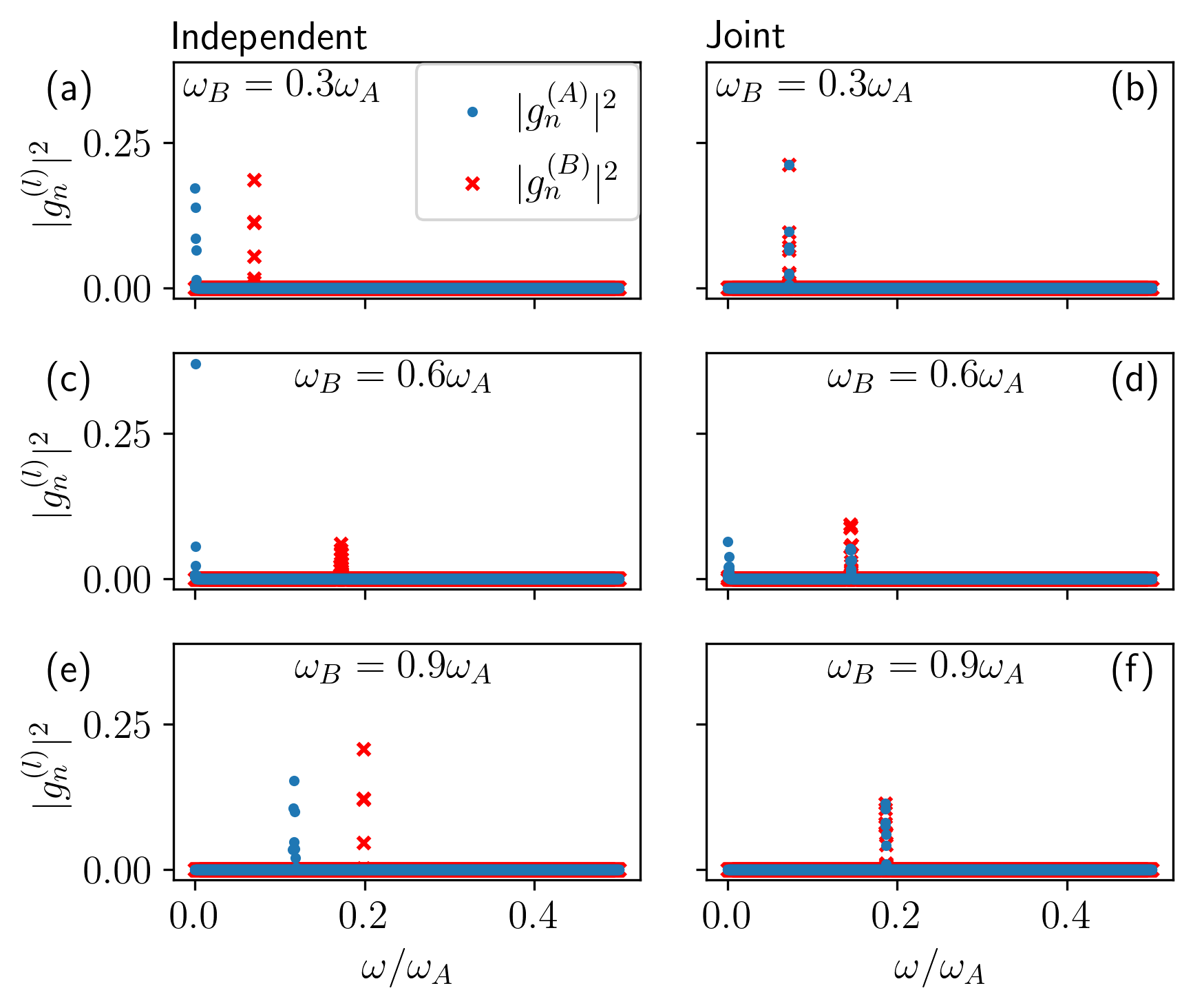
Figure 8: $|g_{n}^{(l)}|^{2}$, for $l=A$ (blue circles) and $l=B$ (red crosses), as a function of the frequency $\omega=n\Omega$, found in specific points of Fig. 4, i.e., in the moderate damping case. The left (right) column is relative to the independent (joint) case, while each row corresponds to a different value of $\omega_{B}$ reported on each panel. (a,b,e,f) correspond to the maximum power driving, while (c) corresponds to the $(\tilde{\sigma},|\tilde{P}|)=(0.13,0.021)$ point, and (d) to $(\tilde{\sigma},-\tilde{P})=(0.12,0.065)$.

In Fig. 8 we report the square modulus of the optimal driving coefficients $|g_{n}^{(l)}|^{2}$, as a function of the frequency $\omega=n\Omega$, relative to specific points in Fig. 4. In particular, the left (right) column is relative to the independent (joint) case, while each row corresponds to a different value of $\omega_{B}$ (reported on each panel). Panels (a,b,e,f) report the square modulus of the coefficients in the maximum power case, while panel (c,d) report a case with low power and low entropy production. In particular, Panel (c) corresponds to the $(\tilde{\sigma},|\tilde{P}|)=(0.13,0.021)$ point, while Panel (d) corresponds to $(\tilde{\sigma},|\tilde{P}|)=(0.12,0.065)$. Since we are optimizing over 5.000 values of $\omega$, points that appear to be “vertical” correspond to extremely similar frequencies, and thus we consider them as a single frequency (it is likely that optimizing for more steps or decreasing the learning rate could yield exactly a single frequency). As discussed in the main text, we see that the independent case always finds two distinct frequencies for each QHO [see panels (a,c,e)]. On the other hand, the joint case at maximum power is always given by a single frequency [see panels (b,f)]. Along the rest of the Pareto front, the joint case is also always optimal at a single frequency, except for the low power regime at $\omega_{B}=0.6\omega_{A}$, where two frequencies become optimal. Such an example is reported in Panel (d). Interestingly, as opposed to the independent case where each QHO is operated at a distinct frequency, here QHO $A$ is driven at both frequencies.

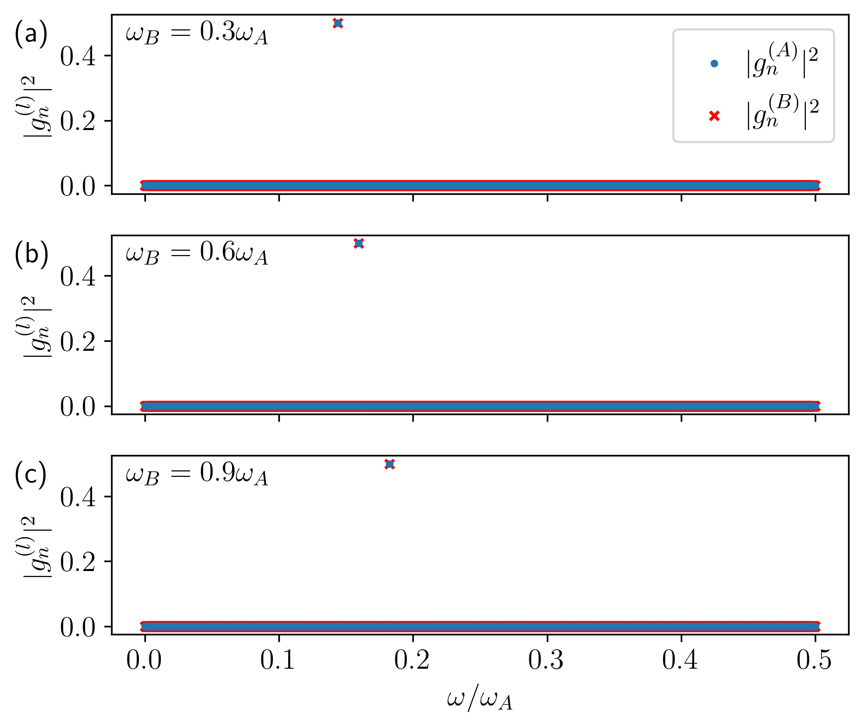
Figure 9: $|g_{n}^{(l)}|^{2}$, for $l=A$ (blue circles) and $l=B$ (red crosses), as a function of the frequency $\omega=n\Omega$, found in specific points of Fig. 5, i.e., in the ultra-strong damping case. Only the joint case is considered since the independent case does not operate as a heat engine in this regime. Each row corresponds to a different value of $\omega_{B}$ reported on each panel. All plots correspond to the driving that maximizes the power.

In Fig. 9 we report the same data, i.e., the square of the driving coefficients as a function of the frequency, relative to the maximum power points in Fig. 5. Only the joint case is analyzed since the independent case does not operate as a heat engine in this regime. Each row corresponds to a different value of $\omega_{B}$ (reported on each panel). As discussed in the main text and confirmed in Fig. 5, in all these cases the optimal driving is monochromatic and occurs at $\omega=\bar{\omega}$.

Appendix F Logarithmic negativity

In this Section we provide some details on the evaluation of possible fingerprint of entanglement in the WM in the case of bath-mediated correlations. To this end we restrict the analysis to the $\nu=2$ reservoir, the one responsible for mediating correlations, since the other is only weakly coupled to the quantum system.

We recall that the logarithmic negativity [55, 56, 30, 32] is defined as

$$E_{n}\equiv{\rm Max}\big{[}0,-\log(2\tilde{\nu})\big{]}~{}.$$ (114)

A finite $E_{n}$ is a fingerprint of entanglement. Therefore it is required that $\tilde{\nu}<1/2$, where $\tilde{\nu}$ is the so-called symplectic eigenvalue of the partial transposed density matrix [55]. For gaussian states this quantity can be written as [30, 32]

$$2\tilde{\nu}^{2}=\Delta-\sqrt{\Delta^{2}-4\det(\Sigma)}~{}.$$ (115)

In the above equation we have introduced the covariance matrix

$$\Sigma=\left(\begin{array}[]{cc}\alpha&\gamma\\ \gamma^{t}&\beta\end{array}\right)$$ (118)

where the two-by-two submatrices $\alpha$ and $\beta$ refer to the $A$ and $B$ QHO correlators, while $\gamma$ refers to mixed ones. In particular, these are given by

$$\alpha=\left(\begin{array}[]{cc}\langle x_{A}^{(0)}(t)x_{A}^{(0)}(t)\rangle_{s}&\langle x_{A}^{(0)}(t)p_{A}^{(0)}(t)\rangle_{s}\\ \langle p_{A}^{(0)}(t)x_{A}^{(0)}(t)\rangle_{s}&\langle p_{A}^{(0)}(t)p_{A}^{(0)}(t)\rangle_{s}\end{array}\right)$$ (121)

$$\beta=\left(\begin{array}[]{cc}\langle x_{B}^{(0)}(t)x_{B}^{(0)}(t)\rangle_{s}&\langle x_{B}^{(0)}(t)p_{B}^{(0)}(t)\rangle_{s}\\ \langle p_{B}^{(0)}(t)x_{B}^{(0)}(t)\rangle_{s}&\langle p_{B}^{(0)}(t)p_{B}^{(0)}(t)\rangle_{s}\end{array}\right)$$ (124)

and

$$\gamma=\left(\begin{array}[]{cc}\langle x_{A}^{(0)}(t)x_{B}^{(0)}(t)\rangle_{s}&\langle x_{A}^{(0)}(t)p_{B}^{(0)}(t)\rangle_{s}\\ \langle p_{A}^{(0)}(t)x_{B}^{(0)}(t)\rangle_{s}&\langle p_{A}^{(0)}(t)p_{B}^{(0)}(t)\rangle_{s}\end{array}\right)$$ (127)

in terms of equal time symmetrized (see the subscript_s) position and momentum correlators. Here, we are interested in the long time behaviour, when a stationary regime has been reached, therefore these quantities do not depend on time. In Eq. (115) we have also introduced

$$\Delta=\det(\alpha)+\det(\beta)-2\det(\gamma).$$ (128)

The symmetrized position and momentum correlators can be written in terms of the imaginary part of the response function ${\bm{\chi}_{2}}$ as

$$\langle x^{(0)}_{l}(t)x^{(0)}_{l^{\prime}}(t)\rangle_{s}=\int_{-\infty}^{+\infty}\frac{{\rm d}\omega}{2\pi m}{\chi_{2}^{(ll^{\prime})}}^{\prime\prime}(\omega)\coth\left(\frac{\omega}{2T_{2}}\right)$$

$$\langle p^{(0)}_{l}(t)p^{(0)}_{l^{\prime}}(t)\rangle_{s}=m\int_{-\infty}^{+\infty}\frac{{\rm d}\omega}{2\pi}{\omega^{2}\chi_{2}^{(ll^{\prime})}}^{\prime\prime}(\omega)\coth\left(\frac{\omega}{2T_{2}}\right),$$ (129)

while all other correlators of the form $\langle x^{(0)}_{l}(t)p^{(0)}_{l^{\prime}}(t)\rangle_{s}$ are zero. Therefore, all submatrices $\alpha$, $\beta$, and $\gamma$ have diagonal components only. It is worth to note that the momentum-momentum correlator in Eq. (F) contains a logarithmic divergence at high frequencies and, in general, a cut-off $\omega_{c}$ in the Ohmic Drude form of the damping function $\gamma_{2}(\omega)$.. However, it is possible to demonstrate (not shown) that $\tilde{\nu}$, and thus also $E_{n}$, have finite values in the $\omega_{c}\to+\infty$ limit. Indeed, even though $\tilde{\nu}$ depends on combinations of position and momentum correlators, all logarithmic divergences cancel out and thus $\tilde{\nu}$ is a well-behaved expression also when $\omega_{c}\to+\infty$.

Inspecting Eqs.(115)-(F), together with Eq. (III.2), one can evaluate $E_{n}$ in Eq. (114). A representative example of $E_{n}$ for the moderate damping case $\gamma_{2}=0.1\omega_{A}$, and for different $\omega_{B}/\omega_{A}$, is reported in Fig. 10 showing that it is finite at sufficiently low temperatures, while it vanishes at higher ones.

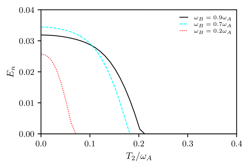
Figure 10: Logarithmic negativity $E_{n}$ as a function of the normalized temperature $T_{2}/\omega_{A}$ for $\gamma_{2}=0.1\omega_{A}$. Different curves refer to different values of $\omega_{B}/\omega_{A}$.

A closed expression for $\tilde{\nu}$ can be found in the strong damping regime. Indeed, exploiting Eq. (31) one can arrive at analytical expressions for the correlators in Eq. (F). In doing so, a useful relation is

$$\lim_{\eta_{0}\to 0}\omega\coth\left(\frac{\omega}{2T_{2}}\right)\frac{\eta_{0}}{\omega^{2}+\eta_{0}^{2}}\to 2\pi T_{2}\delta(\omega)~{},$$ (130)

which implies that the position-position correlator takes contributions both from $\omega\sim 0$ and from $\omega\sim\bar{\omega}$, while the momentum-momentum one is governed by contributions close to $\bar{\omega}$. After some passages, one eventually arrives at

$$\tilde{\nu}^{2}=\frac{\bar{\omega}^{4}\coth^{2}(y)}{4y\omega_{A}^{2}\omega_{B}^{2}}\frac{1}{\coth(y)+\frac{(\omega_{B}^{2}-\omega_{A}^{2})^{2}}{4y\omega_{A}^{2}\omega_{B}^{2}}}\,,$$ (131)

with $y=\bar{\omega}/(2T_{2})$. Recalling that finite entanglement is expected for $\tilde{\nu}<1/2$, this will define the critical temperature $T^{*}$ in the asymptotic regime of large $\gamma_{2}$: $\tilde{\nu}(t^{*})=1/2$.

References

- [1] C. Huygens, Letters to de Sluse, (letters; no. 1333 of 24 February 1665, no. 1335 of 26 February 1665, no. 1345 of 6 March 1665) (Societe Hollandaise Des Sciences, Martinus Nijho, 1895).
- [2] J. Swift, Gulliver’s travels (Motte, London, 1726).
- [3] A. Cavagna and I. Giardina, Bird Flocks as Condensed Matter, Ann. Rev. Condens. Matter Phys. 5, 183 (2014).
- [4] A. Acin et al., The quantum technologies roadmap: a European community view, New J. Phys. 20, 080201 (2018).
- [5] G. Benenti, G. Casati, D. Rossini, and G. Strini, Principles of quantum computation and information (World Scientific, Singapore, 2019).
- [6] R. Kosloff, Quantum Thermodynamics: A Dynamical Viewpoint, Entropy 15, 2100 (2013).
- [7] D. Gelbwaser-Klimovsky, W. Niedenzu, and G. Kurizki, Thermodynamics of Quantum Systems Under Dynamical Control, in Advances In Atomic, Molecular, and Optical Physics, Vol. 64, edited by E. Arimondo, C. C. Lin, and S. F. Yelin (Academic Press, 2015), p. 329.
- [8] B. Sothmann, R. Sánchez, and A. N. Jordan, Thermoelectric energy harvesting with quantum dots, Nanotechnology 26, 032001 (2015).
- [9] S. Vinjanampathy and J. Anders, Quantum thermodynamics, Contemp. Phys. 57, 545 (2016).
- [10] J. Goold, M. Huber, A. Riera, L. del Rio, and P. Skrzypczyk, The role of quantum information in thermodynamics–a topical review, J. Phys. A: Math. Theor. 49, 143001 (2016).
- [11] G. Benenti, G. Casati, K. Saito, and R. S. Whitney, Fundamental aspects of steady-state conversion of heat to work at the nanoscale, Phys. Rep. 694, 1 (2017).
- [12] G. T. Landi and M. Paternostro, Irreversible entropy production: From classical to quantum, Rev. Mod. Phys. 93, 035008 (2021).
- [13] J. P. Pekola and B. Karimi, Colloquium: Quantum heat transport in condensed matter systems, Rev. Mod. Phys. 93, 041001 (2021).
- [14] L. Arrachea, Energy dynamics, heat production and heat-work conversion with qubits: toward the development of quantum machines, Rep. Prog. Phys. 86, 036501 (2023).
- [15] G. T. Landi, D. Poletti, and G. Schaller, Non-equilibrium boundary driven quantum systems: models, methods and properties, Rev. Mod. Phys. 94, 0945006 (2022).
- [16] L. M. Cangemi, C. Bhadra, and A. Levy, Quantum Engines and Refrigerators, ArXiv:2302.00726 (2023).
- [17] R. Lopez, J. S. Lim, and K. W. Kim, An optimal superconducting hybrid machine, ArXiv:2209.09654 (2022).
- [18] R. Lopez, P. Simon, and M. Lee, Heat and charge transport in interacting nanoconductors driven by time-modulated temperatures, ArXiv:2308.03426 (2023).
- [19] M. Campisi and R. Fazio, The power of a critical heat engine, Nat. Commun. 7, 11895 (2016).
- [20] J. Jaramillo, M. Beau, and A. del Campo, Quantum supremacy of many-particle thermal machines, New J. Phys. 18, 075019 (2016).
- [21] H. Vroylandt, M. Esposito, and G. Verley, Collective effects enhancing power and efficiency, Europhys. Lett. 120, 30009 (2018).
- [22] A. Ü. C. Hardal, M. Paternostro, and Ö. E. Müstecaplıoğlu, Phase-space interference in extensive and nonextensive quantum heat engines, Phys. Rev. E 97, 042127 (2018).
- [23] W. Niedenzu and G. Kurizki, Cooperative many-body enhancement of quantum thermal machine power, New J. Phys. 20, 113038 (2018).
- [24] D. Gelbwaser-Klimovsky, W. Kopylov, and G. Schaller, Cooperative efficiency boost for quantum heat engines, Phys. Rev. A 99, 022129 (2019).
- [25] C. L. Latune, I. Sinayskiy, and F. Petruccione, Collective heat capacity for quantum thermometry and quantum engine enhancements, New J. Phys. 22, 083049 (2020).
- [26] G. Watanabe, B. P. Venkatesh, P. Talkner, M.-J. Hwang, and A. del Campo, Quantum Statistical Enhancement of the Collective Performance of Multiple Bosonic Engines, Phys. Rev. Lett. 124, 210603 (2020).
- [27] L. da Silva Souza, G. Manzano, R. Fazio, and F. Iemini, Collective effects on the performance and stability of quantum heat engines, Phys. Rev. E 106, 014143 (2022).
- [28] S. Kamimura, H. Hakoshima, Y. Matsuzaki, K. Yoshida, and Y. Tokura, Quantum-Enhanced Heat Engine Based on Superabsorption, Phys. Rev. Lett. 128, 180602 (2022).
- [29] S. Kamimura, K. Yoshida, Y. Tokura, and Y. Matsuzaki, Universal Scaling Bounds on a Quantum Heat Current, Phys. Rev. Lett. 131, 090401 (2023).
- [30] J. P. Paz and A. J. Roncaglia, Dynamical phases for the evolution of the entanglement between two oscillators coupled to the same environment, Phys. Rev. A 79, 032102 (2009).
- [31] F. Galve, G. L. Giorgi, and R. Zambrini, Entanglement dynamics of nonidentical oscillators under decohering environments, Phys. Rev. A 81, 062117 (2010).
- [32] L. A. Correa, A. A. Valido, and D. Alonso, Asymptotic discord and entanglement of nonresonant harmonic oscillators under weak and strong dissipation, Phys. Rev. A 86, 012110 (2012).
- [33] L. Henriet, Environment-induced synchronization of two quantum oscillators, Phys. Rev. A 100, 022119 (2019).
- [34] L. A. Correa, J. P. Palao, G. Adesso, and D. Alonso, Performance bound for quantum absorption refrigerators, Phys. Rev. E 87, 042131 (2013).
- [35] A. A. Valido, A. Ruiz, and D. Alonso, Quantum correlations and energy currents across three dissipative oscillators, Phys. Rev. E 91, 062123 (2015).
- [36] C. Henkel, Heat Transfer and Entanglement–Non-Equilibrium Correlation Spectra of Two Quantum Oscillators, Annalen der Physik 533, 2100089 (2021).
- [37] C. G. Feyisa and H. H. Jen, A photonic engine fueled by quantum-correlated atoms, arXiv: 2307.16726 (2023).
- [38] X. Li, J. Marino, D. E. Chang, and B. Flebus, A solid-state platform for cooperative quantum phenomena, ArXiv: 2309.08991 (2023).
- [39] Y. Ashida and T. Sagawa, Learning the best nanoscale heat engines through evolving network topology, Commun. Phys. 4, 45 (2021).
- [40] P. A. Erdman, A. Rolandi, P. Abiuso, M. Perarnau-Llobet, and F. Noé, Pareto-optimal cycles for power, efficiency and fluctuations of quantum heat engines using reinforcement learning, Phys. Rev. Research 5, L022017 (2023).
- [41] P. A. Erdman and F. Noé, Model-free optimization of power/efficiency tradeoffs in quantum thermal machines using reinforcement learning, PNAS Nexus 2, pgad248 (2023).
- [42] P. Sgroi, G. M. Palma, and M. Paternostro, Reinforcement learning approach to nonequilibrium quantum thermodynamics, Phys. Rev. Lett. 126, 020601 (2021).
- [43] P. A. Erdman and F. Noé, Identifying optimal cycles in quantum thermal machines with reinforcement-learning, npj Quantum Inf. 8, 1 (2022).
- [44] I. Khait, J. Carrasquilla, and D. Segal, Optimal control of quantum thermal machines using machine learning, Phys. Rev. Research 4, L012029 (2022).
- [45] A. O. Caldeira and A. J. Leggett, Quantum tunnelling in a dissipative system, Ann. Phys. 149, 374 (1983).
- [46] U. Weiss, Quantum Dissipative Systems - 5th Edition (World Scientific, Singapore, 2021).
- [47] E. Aurell, Characteristic functions of quantum heat with baths at different temperatures, Phys. Rev. E 97, 062117 (2018).
- [48] M. Carrega, L. M. Cangemi, G. De Filippis, V. Cataudella, G. Benenti, and M. Sassetti, Engineering Dynamical Couplings for Quantum Thermodynamic Tasks, PRX Quantum 3, 010323 (2022).
- [49] F. Cavaliere, M. Carrega, G. De Filippis, V. Cataudella, G. Benenti, and M. Sassetti, Dynamical heat engines with non-Markovian reservoirs, Phys. Rev. Research 4, 033233 (2022).
- [50] F. Cavaliere, L. Razzoli, M. Carrega, G. Benenti, and M. Sassetti, Hybrid quantum thermal machines with dynamical couplings, iScience 26, 106235 (2023).
- [51] V. Pareto, Manuale di Economia Politica (Società Editrice Libraria, Milan, 1906). Translated into English as Manual of Political Economy (Oxford University Press, Oxford, 2014).
- [52] V. Patel, V. Savsani, and A. Mudgal, Many-objective thermodynamic optimization of Stirling heat engine, Energy 125, 629 (2017).
- [53] A. P. Solon and J. M. Horowitz, Phase transition in protocols minimizing work fluctuations, Phys. Rev. Lett. 120, 180605 (2018).
- [54] J. Gonzalez-Ayala, J. Guo, A. Medina, J. M. M. Roco, and A. Calvo Hernández, Energetic Self-Optimization Induced by Stability in Low-Dissipation Heat Engines, Phys. Rev. Lett. 124, 050603 (2020).
- [55] R. Simon, Peres-Horodecki Separability Criterion for Continuous Variable Systems, Phys. Rev. Lett. 84, 2726 (2000).
- [56] A. Serafini, F. Illuminati, M. G. A. Paris, and S. De Siena, Entanglement and purity of two-mode Gaussian states in noisy channels, Phys. Rev. A 69, 022318 (2004).
- [57] J. P. Paz and A. J. Roncaglia, Dynamics of the Entanglement between Two Oscillators in the Same Environment, Phys. Rev. Lett. 100, 220401 (2008).
- [58] G. Vidal and R. F. Werner, Computable measure of entanglement, Phys. Rev. A 65, 032314 (2002).
- [59] M. Wiedmann, J. T. Stockburger, and J. Ankerhold, Non-Markovian dynamics of a quantum heat engine: out-of- equilibrium operation and thermal coupling control, New J. Phys. 22, 033007 (2020).
- [60] M. Esposito, K. Lindenberg, and C. Van den Broeck, Entropy production as correlation between system and reservoir, New J. Phys. 12, 013013 (2010).
- [61] M. Thorwart, E. Paladino, and M. Grifoni, Dynamics of the spin-boson model with a structured environment, Chem. Phys. 296, 333 (2004).
- [62] E. Paladino, A. G. Maugeri, M. Sassetti, G. Falci, and U. Weiss, Structured environments in solid state systems: crossover from Gaussian to non-Gaussian behavior, Physica E 40, 198 (2007).
- [63] J. Iles-Smith, N. Lambert, and A. Nazir, Environmental dynamics, correlations, and the emergence of noncanonical equilibrium states in open quantum systems, Phys. Rev. A 90, 032114 (2014).
- [64] S. Gröblacher, A. Trubarov, N. Prigge, G. D. Cole, M. Aspelmeyer, and J. Eisert, Observation of non-Markovian micromechanical Brownian motion, Nat. Commun. 6, 7606 (2015).
- [65] G. Torre, W. Roga, and F. Illuminati, Non-Markovianity of Gaussian Channels, Phys. Rev. Lett. 115, 070401 (2015).
- [66] A. Cottet, M. C. Dartiailh, M. M. Desjardins, T. Cubaynes, L. C. Contamin, M. Delbecq, J. J. Viennot, L. E. Bruhat, B. Douçot, and T. Kontos, Cavity QED with hybrid nanocircuits: from atomic-like physics to condensed matter phenomena, J. Phys.: Condens. Matter 29, 433002 (2017).
- [67] A. Calzona and M. Carrega, Multi-mode architectures for noise-resilient superconducting qubits, Supercond. Sci. Technol. 36, 023001 (2023).
- [68] B. Peropadre, D. Zueco, F. Wulschner, F. Deppe, A. Marx, R. Gross, and J. J. García-Ripoll, Tunable coupling engineering between superconducting resonators: From sidebands to effective gauge fields, Phys. Rev. B 87, 13450 (2013).
- [69] I. C. Rodrigues, D. Bothner, and G. A. Steele, Coupling microwave photons to a mechanical resonator using quantum interference, Nat. Commun. 10, 5359 (2019).
- [70] We have investigated other temperature configurations in the engine working mode and no qualitative changes have been observed.
- [71] L. F. Seoane and R. Solé, Multiobjective optimization and phase transitions, in Proceedings of ECCS 2014, edited by S. Battiston, F. De Pellegrini, G. Caldarelli, and E. Merelli, p. 259 (Springer, Cham, 2016).
- [72] D. P. Kingma and J. Ba, Adam: A method for stochastic optimization, arXiv:1412.6980 (2017).
- [73] A. Paszke et al., PyTorch: An imperative style, high-performance deep learning library, in Advances in Neural Information Processing Systems 32, edited by H. Wallach, H. Larochelle, A. Beygelzimer, F. d’Alché-Buc, E. Fox, and R. Garnett (NeurIPS, 2019).
- [74] J. C. Platt and A. H. Barr, Constrained differential optimization, in Neural Information Processing Systems 0, edited by D. Anderson (American Institute of Physics, 1987), p. 612.
- [75] P. Pietzonka and U. Seifert, Universal trade-off between power, efficiency, and constancy in steady-state heat engines, Phys. Rev. Lett. 120, 190602 (2018).
- [76] T. Koyuk, U. Seifert, and P. Pietzonka, A generalization of the thermodynamic uncertainty relation to periodically driven systems, J. Phys. A: Math. Theor. 52, 02LT02 (2019).
- [77] K. Brandner, T. Hanazato, and K. Saito, Thermodynamic Bounds on Precision in Ballistic Multiterminal Transport, Phys. Rev. Lett. 120, 090601 (2018).
- [78] L. M. Cangemi, V. Cataudella, G. Benenti, M. Sassetti, and G. De Filippis, Violation of TUR in a periodically driven work-to-work converter from weak to strong dissipationPhys. Rev. B 102, 165418 (2020).
- [79] L. M. Cangemi, M. Carrega, A. De Candia, V. Cataudella, G. De Filippis, M. Sassetti, and G. Benenti, Optimal energy conversion through antiadiabatic driving breaking time-reversal symmetry, Phys. Rev. Research 3, 013237 (2021).
- [80] G.-L. Ingold, Path Integrals and Their Application to Dissipative Quantum Systems, in Coherent Evolution in Noisy Environments. Lecture Notes in Physics, Vol. 611, edited by A. Buchleitner and K. Hornberger (Springer Berlin, Heidelberg, 2002), p. 1.