Flux-conserving directed percolation

Abstract

We discuss a model for directed percolation in which the flux of material along each bond is a dynamical variable. The model includes a physically significant limiting case where the total flux of material is conserved. We show that the distribution of fluxes is asymptotic to a power law at small fluxes. We give an implicit equation for the exponent, in terms of probabilities characterising site occupations. In one dimension the site occupations are exactly independent, and the model is exactly solvable. In two dimensions, the independent-occupation assumption gives a good approximation. We explore the relationship between this model and traditional models for directed percolation.

1 Introduction

Percolation problems were introduced by Broadbent and Hammersley in 1957 [1]. Their paper motivated the study of percolation [2] by a discussion of fluids passing through a disordered medium, such as water penetrating through limestone. Forced flow of a liquid through a porous medium is central to many interesting and technologically important processes involving elution from, or absorption by, random media, such as leaching of salts from soil, extraction of oil or gas from reservoirs, brewing coffee, or the operation of chromatography columns, which stimulated the study of directed percolation. There is a vast literature treating the standard models of directed percolation, reviewed in [3], and [4, 5, 6, 7, 8, 10, 9, 11, 12, 13, 14, 15, 16] are indicative of the breadth of different approaches to directed percolation, and of its wide range of applications. The standard percolation models (such as bond percolation on a lattice) do not take into account the mass conservation of a flowing liquid. In this paper we consider a generalisation of directed percolation, which includes the flux in a bond as a dynamical variable. If the fluxes are ignored, and only the occupancy of bonds is considered, then the standard directed percolation model occurs as a particular special case. Our generalised model includes a flux-conserving case which can describe the forced flow of a liquid through a random medium, and we shall consider this in some detail. We demonstrate that aspects of the subset of models which represents elution by a flux-conserving fluid are exactly solvable in one dimension, extending some results obtained (in another context) in [17]. Our generalised model has some similarity to the Scheidegger model for the distribution of river catchment basins [18, 19], which will be discussed in the conclusions. Another, more distantly related, class of models which quantify directed transport in random media is described in [20, 21].

The percolation model introduced by Broadbent and Hammersley uses the idea of ‘wetted’ bonds. Here we extend this binary notion of wetting by modelling the flux $\phi$ of liquid through each bond and the probability distribution of such fluxes. We argue that, for a quite general class of flux-conserving process which involve a forced flow through a disordered medium, the distribution of the fluxes has some universal characteristics. After penetrating a sufficient distance into the network, the probability density $P(\phi)$ for the flux $\phi$ in a channel may approach a stationary distribution, with a power-law form at small values of $\phi$:

$$P(\phi)\sim\phi^{-\alpha}\ .$$ (1)

The existence of power laws is usually associated with critical phenomena, however the power-law distribution described by equation (1) is a robust feature, which does not depend upon tuning the model to criticality. We argue that the mechanism determining the power law is very general, and that power-law distributions of small fluxes are a robust feature of the model.

Section 2 defines our model, in both one and two dimensions. Our model includes both a ‘skeleton’ of wetted bonds, and the flux of material, $\phi$, carried in each wetted bond. The skeleton is defined by three probabilities: a wetted channel continues with probability $p_{1}$, splits into $K$ channels with probability $p_{2}$, and terminates with probability $p_{0}$. The flux carried by a bond which splits is distributed so that a fraction $r_{k}$ flows into each branch, with $r_{1}+\ldots+r_{K}=1$, where $r_{k}\in[0,1]$. We emphasise cases where there are only $K=2$ branches, and where the two branches carry fixed fractions of the total flux, denoted by $r$ and $1-r$. Accounting for the relation $p_{0}+p_{1}+p_{2}=1$, the model then has three independent parameters, $p_{0}$, $p_{2}$ and $r$. The flux-conserving case is the $p_{0}=0$ subspace. The model which was considered in [17] is the one-dimensional, flux-conserving case.

Section 3 considers the distribution of fluxes in the mass-conserving case in some detail. It is shown that, for small values of the flux, the probability distribution function (PDF) of the flux is asymptotic to a power law described by equation (1). We obtain an exact equation for the exponent $\alpha$ of this power law, in terms of some probabilities, $P_{j}$ which characterise the occupation of lattice sites.

The bond skeleton is characterised by the probability $f$ that a given bond is occupied. In section 4 this is calculated under the assumption that the occupation of sites is statistically independent, and we find very good agreement between theory and numerical experiment. Section 5 estimates the probabilities $P_{j}$ which define the equation for $\alpha$ using the same approach, and we compare empirically determined values for the exponent $\alpha$ with those obtained from both numerical and theoretical estimates of the $P_{j}$.

In section 6 we consider the extent to which the independent-occupancy approximation is exact. We demonstrate two results which indicate that it is exact in the one-dimensional version of the model. We find that, in the two-dimensional case, this is a very good approximation, but not exact.

Section 7 discusses the relationship between our system and the standard model for directed percolation. By varying the parameter $p_{0}$ we can induce a percolation transition in our model, which can be regarded as a consequence of large voids appearing between the active bonds. In sub-section 7.1 we investigate where the transition lies in the parameter space of our model. Our model can be thought of in terms of a combination of ‘bond’ and ‘site’ deletion processes, and section 7.1 also discuss the relationship between our system and a model for mixed site and bond percolation, discussed in [16]. Sub-section 7.2 presents some numerical evidence that the the critical exponents describing the structure of the skeleton are the same as for the usual directed percolation model. In section 7.3 we present some results on the distribution of void sizes.

Finally section 8 summarises and discusses the implications of our results, including a model for the slow elution of material by percolation.

2 Definition of the model

We define discrete dynamical processes, with an iteration number, $j$. Incrementing $j$ can be thought of as advancing time, but in the physical contexts described in the Introduction, increasing $j$ represents moving downstream in the forced flow. Because the iteration index can be interpreted as a discrete time, our one or two dimensional systems are comparable to standard models for directed percolation in $1+1$ dimensions or $2+1$ dimensions, respectively.

2.1 One-dimensional model

We consider a bi-partite lattice. At even iteration number $j$, only even sites are occupied. The dynamics always moves an occupied site by one unit left or right, so that for odd iteration number, only the odd sites may be occupied. Every occupied site, index $i$, is associated with a flux, $\phi_{i}(j)$, at iteration $j$.

First consider the dynamics of the site occupations. At each iteration, an occupied site is annihilated with probability $p_{0}$, or moves either right or left with equal probabilities $p_{1}/2$, or else it splits into $K=2$ branches with probability $p_{2}$.

The corresponding dynamics of the fluxes is as follows. If a site is annihilated its flux disappears. When transitions bring two occupied sites to the same position, their fluxes combine, and if the site branches, then its flux is divided. So values of the flux are changed by two possible processes:

$${\rm coalescence}: \phi_{i}(j+1)=\phi_{i-1}(j)+\phi_{i+1}(j)$$

$$\ \ \ \ \ {\rm splitting}: \phi_{i-1}(j+1)=r_{-}\phi_{i}(j)\ ,\ \ \ \phi_{i+1}(j+1)=r_{+}\phi_{i}(j)$$ (2)

where either $(r_{+},r_{-})=(r,1-r)$ or $(r_{+},r_{-})=(1-r,r)$, both cases with probability equal to one-half. The model is illustrated schematically in figure 1. More generally, we can make $r\in[0,1]$ a random variable, chosen independently for every bifurcation, with a PDF which is symmetric about $\frac{1}{2}$.

Figure 1: The model is defined on a bi-partite lattice. Only even sites (red) are occupied at even-numbered iterations, only odd sites (blue) during odd iterations. At each iteration every occupied site is either removed (probability $p_{0}$), moves to one of its nearest neighbours (probability $p_{1}$), or else splits into $K=2$ daughters (probability $p_{2}$). The flux $\phi$ carried by an occupied site moves with it, unless the site is removed, in which case the flux disappears. When two fluxes are moved to the same site, they are added.

The model only describes a volume-preserving flow when the stopping probability $p_{0}$ is equal to zero. This parameter is included for two reasons. The parameter $p_{0}$ is included primarily so that our system encompasses the standard model of directed percolation. In addition, the case where $p_{0}>0$ can model situations where the solvent disappears, for example by evaporation.

The fluxes at each wetted site can increase (due to coalescence) or decrease (due to splitting), and some sites become unoccupied. The long-time behaviour of the model is characterised by the probability, $f$, that sites are occupied and the distribution of the non-zero values of $\phi$. A nonzero value of $p_{0}$ implies a loss of conservation, which significantly changes the nature of the problem. When $p_{0}$ is large enough, the probability that a site is occupied at long times becomes zero, and as $p_{0}$ decreases, one observes a transition when the probability of occupation becomes strictly positive.

2.2 Two-dimensional model

Consider a model defined on an $2N\times 2N$ square lattice, with sides identified to make a toroidal topology. Every site $(i,j)$ carries a weight $\phi_{ij}$. Initially only sites with $i+j$ even are occupied, with unit weight, so that our model is defined on a bi-partite lattice. The value of $N$ is assumed to be large.

The lattice configuration is then evolved in discrete timesteps. At each site, we choose (with equal probabilities) a move to one of the four nearest neighbour sites. With probability $p_{1}$, all of the flux on $(i,j)$ is moved to the selected neighbour. Alternatively, with probability $p_{2}$, branching onto $K$ nearest neighbours occurs. Note that these moves preserve the bi-partite property, so that at iteration $k$, only sites with $i+j$ having the same parity as $k$ may be occupied.

We investigated two different versions of this model, which we term the two-branch and four-branch models. In the two-branch model, we have $K=2$, and a fraction $1-r$ of the weight at $(i,j)$ is moved to the selected neighbour, and a fraction $r$ is moved in the reciprocal direction. All of the random choices are independent. The model has three parameters of interest, $p_{2}$, $p_{0}$ and $r$.

In the four-branch model, there is branching to all of the nearest neighbour sites, so that $K=4$. The fractional weights for each branch are defined by four numbers, $\{r_{1},r_{2},r_{3},r_{4}\}$, with $r_{1}+r_{2}+r_{3}+r_{4}=1$.

Figure 2: In two dimensions, when the flux at an occupied site splits there may be up to four branches. We consider two cases in some detail. In the two-branch version of the model there are two branches, which go in opposite directions, either horizontal or vertical, with equal probability. In the four-branch model, where branching events reach all nearest neighbours, with the locations of the weights $r_{1},r_{2},r_{3},r_{4}$ randomly assigned.

3 Power-law distribution of fluxes in the mass-conserving case

In the following, Sections 3, 4, 5 and 6, we consider exclusively the mass conserving case, with $p_{0}=0$. To simplify the notation, we will set, in these sections, $p=p_{2}$, so that $p_{1}=(1-p)$.

We argue here that the distribution of fluxes $P(\phi)$ has a power-law behaviour in the limit as $\phi\to 0$ (with the exponent in (1) satisfying $\alpha<1$, so that the distribution is normalisable). Branching of a channel reduces the flux due to multiplying by a random factor $r_{k}<1$, which we assume to have a known PDF. Because fluxes are added when coalescence of channels occurs, this process increases the flux. We are interested in the distribution of very small values of the flux $\phi$. In this case splitting and coalescence have very different effects. In the case where a channel carries a very small flux, coalescence with another channel will produce a much larger flux (with a value which is typically comparable to the mean flux). Almost all coalescence events will, therefore, remove a very small value of $\phi$, whereas splitting events just reduce its value. The distribution of very small values of $\phi$ is, therefore, the result of a competition between two process: the small values of $\phi$ continue to decrease due to splitting, but they are annihilated by coalescences.

In order to explain why a power-law distribution of the flux is expected, we start by making a change of variables. Instead of considering $\phi$, we consider the probability density function (PDF) of a logarithmic variable, $\psi\equiv\ln\,\phi$. Consider the dynamics of the variable $\psi$ (regarding increasing $\psi$ as a displacement to the right). With every bifurcation of a channel, the points representing the values of $\psi$ are split into $K$ new points, and each one is displaced by $\ln\,r_{k}$. When two channels coalesce, the two values of $\psi$ are replaced by $\psi=\ln\,[\exp(\psi_{1})+\exp(\psi_{2})]$. In the following we shall assume that the PDF $P(\phi)$ is bounded so that the probability of $\phi$ being less than $\phi_{0}$ approaches zero as $\phi_{0}\to 0$. This is consistent with the distribution (1) provided $\alpha<1$. Under this assumption, in the limit as $\phi\to 0$, most coalescences occur with channels carrying a much larger flux. As a consequence, coalescence of a channel with a small flux, $\psi$, is replaced by a value close to that which characterises a typical channel. This picture implies that the variable $\psi$ drifts to the left with each bifurcation, but, in the case of small fluxes, coalescence almost inevitably causes a jump back to a position close to the origin.

Because the equations defining the dynamics of $\psi$ become independent of the value of $\psi$ in the limit as $\psi\to-\infty$, the PDF of $\psi$ should reflect this translational symmetry. In the limit as $\psi\to-\infty$, the PDF of $\psi$ should be asymptotic to an eigenfunction of the translation operator. Because the exponential function is an eigenfunction of a translation operator, we expect that the PDF of $\psi$ has the form

$$P_{\psi}(\psi)\sim\exp(\lambda\psi)\ .$$ (3)

Note that we must have $\lambda>0$ to have a normalisable distribution if this law holds as $\psi\to-\infty$. The corresponding distribution of $\phi$ is then a power law of the form

$$P(\phi)\sim\phi^{-\alpha},\ \ \ \ \alpha=1-\lambda\ .$$ (4)

This is a very general argument indicating that the steady-state distribution of fluxes approaches a power law as we go deeper into the percolation medium, but it does not yield a prediction of the exponent $\alpha$. Figure 3 illustrates numerical simulations of the distribution $P(\phi)$ for the two-dimensional model, demonstrating that it is indeed asymptotic to a power law at small values of $\phi$.

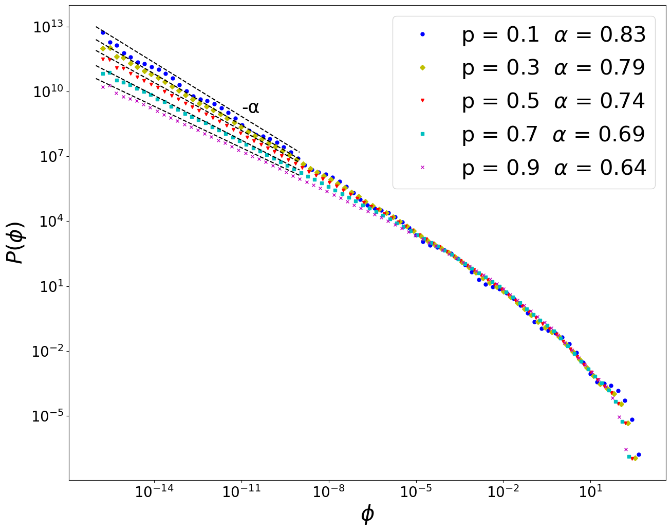
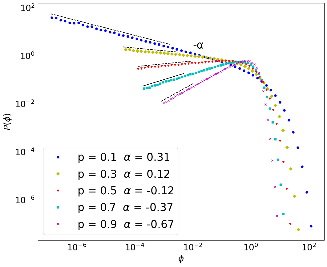
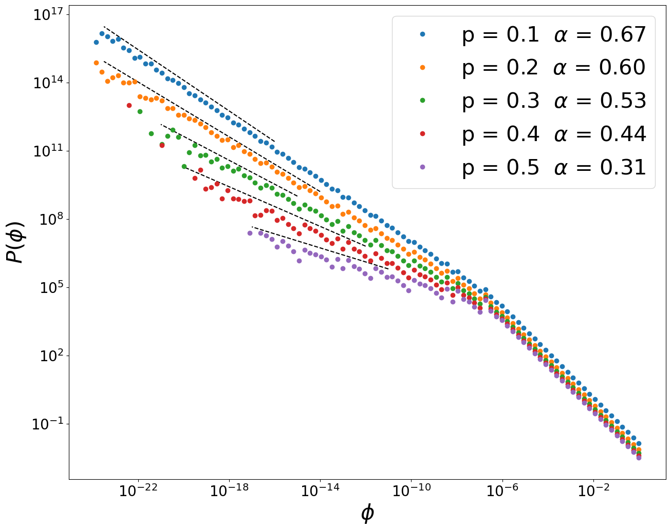
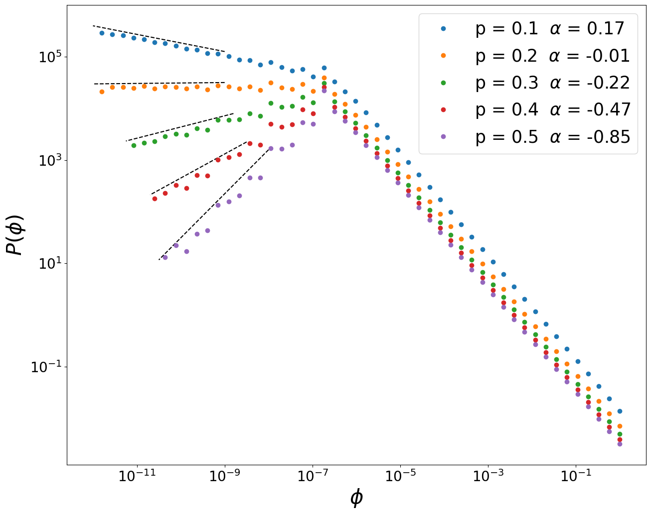
Figure 3: Results of numerical simulations demonstrating that the distribution of flux, $P(\phi)$, is asymptotic to a power law at small $\phi$. We show results for the two-dimensional model. Upper row: two-branch system: each panel illustrates different values of $p$, with $r=0.01$ (left panel) and $r=0.5$ (right panel). Lower row: four-branch system, with $r=0.025$ (left panel) and $r=0.25$ (right panel).

To calculate $\alpha$ we shall determine a master equation for the PDF of the variable $\psi$, valid in the limit as $\psi\to-\infty$. Because coalescence almost inevitably results in the value of $\psi$ making a large jump to the right, we must consider the fate of sites which are occupied and which have not experienced a coalescence for a large number of iterations. The latter requirement is imposed because it is only those sites which have very small values of $\phi$. For this subset of sites we introduce the following probabilities:

$$P_{1} \equiv {\rm\ probability\ of\ moving\ without\ branching\ or\ coalescence}$$

$$P_{2} \equiv {\rm\ probability\ of\ moving\ without\ branching\ and\ undergoing\ coalescence}$$

$$P_{3+k} \equiv {\rm\ probability\ of\ branching\ }K{\rm\ ways,\ with\ }k{\rm\ branches\ undergoing\ coalescence}$$

Note that $P_{1}+P_{2}=1-p$ and $P_{3}+\ldots+P_{3+K}=p$. In practice, when we estimate the $P_{k}$ from numerical simulations, we only accumulate statistics for those sites which have not undergone coalescence in the preceding $N_{\rm thr}$ iterations. We take a sufficiently large value for this threshold such that the $P_{k}$ are insensitive to the value $N_{\rm thr}$.

To describe the asymptotic form of the probability of very small fluxes, we write down an equation for the PDF of $\psi$ at iteration $j+1$, which is valid in the limit as $\psi\to-\infty$. Note that, because events involving coalescence almost always induce a large increase of the flux, they do not contribute to this balance equation for very small values of $\phi$. It follows that it is only events which do not involve coalescence at iteration $j$ which contribute to $P_{\psi}(\psi,j+1)$, when $\psi\to-\infty$: these events are moving without coalescence, leaving $\psi$ unchanged (probability $P_{1}$), or splitting events where some of the daughters escape coalescence (probabilities $P_{3},\ldots,P_{2+K}$). Taking this remark into account, if $P_{\psi}(\psi,j)$ is the PDF of $\psi$ at iteration $j$, then

$$P_{\psi}(\psi,j+1)=P_{1}P_{\psi}(\psi,j)+Q\sum_{k=1}^{K}P_{\psi}(\psi-\ln(r_{k}),j)$$ (6)

with

$$Q=\frac{1}{K}\left[KP_{3}+(K-1)P_{4}+\ldots+P_{K+2}\right]\ .$$ (7)

Seeking a solution of the form (3) which is independent of $j$ gives an exact equation for the exponent $\alpha$:

$$1-P_{1}=Q\sum_{k=1}^{K}r_{k}^{\alpha-1}\ .$$ (8)

In the cases where $K=2$ and where the splitting ratios are $(r,1-r)$), (this includes the one-dimensional model and the two-branch model in two dimensions) equation (8) simplifies to

$$r^{\alpha-1}+(1-r)^{\alpha-1}=F(p)$$ (9)

with

$$F(p)\equiv\frac{1-P_{1}}{Q}=\frac{2(1-P_{1})}{2P_{3}+P_{4}}\ \ \ \ \ \ ({\rm{\bf two-way\ splitting}})\ .$$ (10)

We also simulated a model with $K=4$: when there is a four-way split, we set a weight factor of $r$ for two of the sites (chosen at random), and a factor $1-r$ for the other two sites. In this case, $\alpha$ satisfies equation (9) with

$$F(p)\equiv\frac{1-P_{1}}{2Q}=\frac{(1-P_{1})}{2P_{3}+3P_{4}/2+P_{5}+P_{6}/2}\ \ \ \ \ \ ({\rm{\bf four-way\ splitting}})\ .$$ (11)

4 Occupation probabilities in the mass-conserving case

Here we present calculations for the occupation probability $f$ in the mass-conserving case, $p_{0}=0$, assuming that the occupation of sites is statistically independent of their neighbours. For the sake of simplicity, we set $p=p_{2}$, so $p_{1}=1-p$. We limit the discussion to the two-dimensional models, because the one-dimensional case was treated in [17], where it was shown that the occupation probability is

$${f_{1}}(p)=\frac{4p}{(1+p)^{2}}\ ,$$ (12)

where the sub-index 1 indicates the one-dimensional model.

4.1 Occupation probability: two-dimensional case with double branching

We determine here the probability of occupation in the two-dimensional problem, first with $K=2$ (two-branch model), ${f_{2,2}}(p)$, where the sub-indices indicate the two-dimensional model with two branches and we recall that $p=p_{2}$. Assuming that sites are randomly occupied with probability ${f_{2,2}}$, we estimate the probability $P_{\rm empty}$ that a site will be empty at the next iteration. Note that the probability that one of the four nearby sites makes a transition to reach this site is

$$P_{\rm tr}=\frac{(1+p)}{4}{f_{2,2}}\ .$$ (13)

The probability of the site remaining empty is

$$P_{\rm empty}=\left(1-P_{\rm tr}\right)^{4}=1-{f_{2,2}}\ .$$ (14)

This leads to a cubic equation for ${f_{2,2}}$:

$$1-{f_{2,2}} = \left[1-\left(\frac{1+p}{4}\right){f_{2,2}}\right]^{4}$$ (15)

$$= 1-(1+p){f_{2,2}}+\frac{6}{16}(1+p)^{2}{f_{2,2}}^{2}$$

$$-\frac{1}{16}(1+p)^{3}{f_{2,2}}^{3}+\frac{1}{256}(1+p)^{4}{f_{2,2}}^{4}\ .$$

When $p\ll 1$, this is approximated by $-p{f_{2,2}}+\frac{3}{8}{f_{2,2}}^{2}\sim 0$, so that

$${f_{2,2}}\sim\frac{8}{3}p\ .$$ (16)

The cubic equation arising from (15) can, in fact, be solved by the method of Cardano. Within the interval $p\in(0,1)$, we have only one real root. By this method, the dependence of ${f_{2,2}}$ on $p$ is given by:

$${f_{2,2}}(p)=\frac{4}{3(1+p)}\left[4-\left(\frac{y(p)-x(p)}{1+p}\right)^{1/3}+\left(\frac{x(p)+y(p)}{1+p}\right)^{1/3}\right]\ ,$$ (17)

where

$$x(p)=44-10p\ ,\ \ \ y(p)=6\sqrt{3}\sqrt{p^{2}-8p+18}\ .$$ (18)

The maximum of ${f_{2,2}}(p)$ is ${f_{2,2}}\approx 0.9126$ at $p=1$. Figure 4(a) compares this prediction of the filling probability with the result of numerical simulation. The agreement is very good, but not perfect. In particular, we find that the fractional error is quite large at small values of $p$, as illustrated in panel 4(b). We were not able to determine whether the fractional error eventually approaches zero as $p\to 0$.

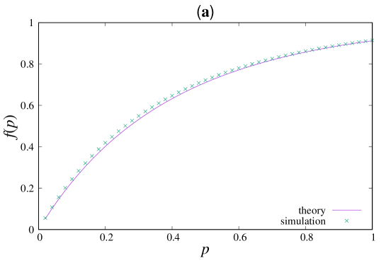
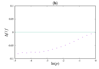
Figure 4: (a) Comparing simulated occupation fraction $f_{2,2}$ for the two-branch model with prediction from independent-occupancy approximation, equations (17) and (18). (b) Shows the fractional error, plotted against $\ln p$. (We defined the fractional error by $\Delta f/f\equiv(f_{\rm th}-f_{\rm num})/\sqrt{f_{\rm th}f_{\rm num}}$, where $f_{\rm th}$ and $f_{\rm num}$ are, respectively, the theoretical and numerically determined values of $f$.)

4.2 Occupation probability: two-dimensional case with fourfold branching

The occupation probability for the four-branch model in two dimensions will be denoted $f_{2,4}$. For this model the transition probability is

$$P_{tr}=\frac{1+3p}{4}f_{2,4}\ .$$ (19)

Then, the cubic equation for $f_{2,4}$ is:

$$1-f_{2,4}=\left[1-\left(\frac{1+3p}{4}\right)f_{2,4}\right]^{4}\ .$$ (20)

Making a comparison with equation (15), we see that $f_{2,4}(p)=f_{2,2}(3p)$, so that the occupation probability in this case is

$$f_{2,4}(p)=\frac{4}{3(1+3p)}\left[4-\left(\frac{y(3p)-x(3p)}{1+3p}\right)^{1/3}+\left(\frac{x(3p)+y(3p)}{1+3p}\right)^{1/3}\right]\ ,$$ (21)

and, when $p\ll 1$, we have $f_{2,4}\sim 8p$. In this case, the maximum value is $f_{2,4}=1$ at $p=1$. Figure 5 compares this prediction of the filling probability with the result of numerical simulation. Again, while the agreement is very good throughout most of the range of $p$, there is a substantial fraction error for small values of $p$.

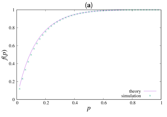
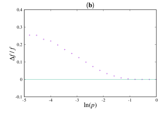
Figure 5: (a) Comparing simulated occupation probability $f_{2,4}$ for the four-branch model with prediction from independent-occupancy approximation, equation (21). (b) Shows the fractional error (defined in the same way as for figure 4), plotted against $\ln p$.

5 Estimates of transition probabilities in the mass-conserving case

In section 3 we presented an exact equation, (8), determining the exponent $\alpha$ in terms of a set of probabilities $P_{k}$, defined by equation (3). In this section we consider these probabilities, comparing numerical simulations with theoretical estimates, where these are available.

We consider different models in turn (including the one-dimensional model, because these probabilities were not given in [17]). In all cases, the theory uses the assumption that the sites are independently occupied with probability $f$, as estimated in section 4. In section 6 we shall argue that this independent-occupation assumption is exact in the one-dimensional case. Accordingly we propose that the formulae for the $P_{k}$ are exact in one dimension.

In the case of the two-dimensional model with two-way splitting, we are able to estimate the $P_{k}$ analytically using the independent-occupation model. We find close agreement with values derived from numerical simulations. In the two-dimensional model with four-way splitting, we are limited to giving values of $P_{k}$ derived from simulations.

5.1 One-dimensional model

A given trail can evolve in several ways at each iteration, with probabilities defined by equation (3). If sites are occupied with probability ${f_{1}}(p)$, we find, using Eq. (12), that there is a transition probability for a trail coalescing with one or other of its two neighbouring sites, given by

$$P_{\rm tr}=\left[\frac{1}{2}(1-p)+p\right]{f_{1}}(p)=\frac{2p}{1+p}$$ (22)

(the term $(1-p)/2$ comes from the case where the neighbouring site does not divide and moves in the direction that creates a collision, and $p$ comes from the case where the neighbouring trail divides).

The probability $P_{1}$ arises from the case where a trail does not divide, and does not collide:

$$P_{1}=(1-p)(1-P_{\rm tr})=\frac{(1-p)^{2}}{1+p}\ .$$ (23)

Similarly

$$P_{2}=(1-p)P_{\rm tr}=\frac{2p(1-p)}{1+p}\ .$$ (24)

In the case where the trail divides, there are two independent chances for the trail to be annihilated, so the probability for both daughter trails to end is

$$P_{5}=p[P_{\rm tr}]^{2}=\frac{4p^{3}}{(1+p)^{2}}\ .$$ (25)

Similarly the probability for both daughter trails to survive is

$$P_{3}=p[1-P_{\rm tr}]^{2}=\frac{p(1-p)^{2}}{(1+p)^{2}}\ .$$ (26)

And because there are two ways in which one daughter trail can continue

$$P_{4}=pP_{\rm tr}[1-P_{\rm tr}]=\frac{4p^{2}(1-p)}{(1+p)^{2}}\ .$$ (27)

Using equations (23) to (27) in equation (9), we find that for the one-dimensional flux-conserving model, $\alpha$ is a solution of

$$r^{\alpha-1}+(1-r)^{\alpha-1}=\frac{3-p}{1-p}$$ (28)

in accord with Equation (2) of [17].

5.2 Two-dimensional model with two branches

Next consider estimates for the transition probabilities for the two-dimensional model with branching into two opposite directions. Again, we use the assumption that the sites are independently occupied, with probability ${f_{2,2}}$, as approximated by equations (17), (18).

First note that a site moves to one of its nearest neighbours with a transition probability, given by equation (13), namely $P_{\rm tr}={f_{2,2}}(p)((1-p)/4+p/2)={f_{2,2}}(p)(1+p)/4$. A site remains un-branched with probability $(1-p)$, and un-combined if there is no other transition into the final site from any of its three other neighbours. Hence

$$P_{1}=(1-p)(1-P_{\rm tr})^{3}\ .$$ (29)

The value of $P_{2}$ is then determined by noting that $1-p=P_{1}+P_{2}$:

$$P_{2}=1-p-P_{1}\ .$$ (30)

If the trajectory branches (with probability $p$), it avoids collision if none of the three nearest neighbours of each of the two new sites make a transition which lands there. Hence

$$P_{3}=p(1-P_{\rm tr})^{6}\ .$$ (31)

Similarly, $P_{5}$ is the probability of an event where neither of the two branches avoids coalescence with at least on one of its three nearest neighbours:

$$P_{5}=p\left[1-(1-P_{\rm tr})^{3}\right]^{2}\ .$$ (32)

To determine $P_{4}$ we can use $P_{3}+P_{4}+P_{5}=p$ to obtain

$$P_{4}=2p(1-P_{\rm tr})^{3}\left[1-(1-P_{\rm tr})^{3}\right]\ .$$ (33)

Figure 6 compares these theoretical estimates for the $P_{k}$ with numerical simulations. The numerical simulations include only sites which had not experienced coalescence in the preceding $N_{\rm thr}=8$ iterations (the parameter $N_{\rm thr}$ was introduced in the paragraph below equation (3)). These simulations show that the true $P_{k}$ values differ slightly from the theoretical expressions, equations (29)-(33), which are plotted in figure 6. The small difference between theory and simulation becomes negligible as $p\to 0$.

We used the theoretical expression for $f(p)$, equations (17), (18), when evaluating equations (29)-(33) for figure 6. Plotting the $P_{k}$ for simulations with $N_{\rm thr}=0$ yields curves which are barely distinguishable from equations (29)-(33), indicating that the small discrepancy is due to the theory neglecting the requirement to exclude sites which have undergone recent collisions, rather than the error in equations (17), (18).

It is impractical to impose very large values of $N_{\rm thr}$ because, as $p\to 1$, very few sites satisfy the requirement to have undergone no coalescences in the last $N_{\rm thr}$ iterations: for $N_{\rm thr}=8$, we found that the probability of an occupied site satisfying this criterion falls from $0.64$ at $p=0.05$ to $0.0013$ at $p=0.75$. Simulations with $N_{\rm thr}=4$ gave points which appear coincident with those for $N_{\rm thr}=8$ when included in figure 6.

Figure 7 provides direct tests of the theoretical prediction for the exponent $\alpha$. We estimated $\alpha$ from simulations with a wide range of values of $r$ and $p$. In the left panel of Fig. 7, we compare the theoretical values of $\alpha$ obtained from equation (9) against numerically estimates, obtained by directly simulating the model: here we used the values of $P_{k}$ obtained from simulations with $N_{\rm thr}=8$. In the right panel we collapse all of the data points onto two plots of $F(p)\equiv(1-P_{1})/Q$, one obtained using equations (29) to (33), the other using values of $P_{k}$ obtained from simulations with $N_{\rm thr}=8$. The former shows small but significant deviations at larger values of $p$. The small dispersion between the symbols gives an indication of the accuracy of our determination of the exponents $\alpha$.

We remark that, if the errors in the approximations underlying equations (29)-(33) and (17), (18) are negligible as $p\to 0$, we can determine the limiting value of $F(p)$ as $p\to 0$. Using these expressions in equation (10) results in

$$\lim_{p\to 0}F(p)=3\ .$$ (34)

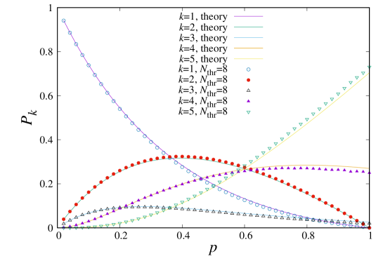
Figure 6: Estimates of the probabilities defined in (3), $P_{k}(p)$, $k=1,\ldots,5$, for the two-dimensional two-branch model. The solid lines are the theoretical predictions, equations (29) to (33). The numerical simulations imposed the requirement that the site has not recently experienced a coalescence in the preceding $N_{\rm thr}=8$ iterations. They differ significantly from the theoretical model as $p\to 1$.

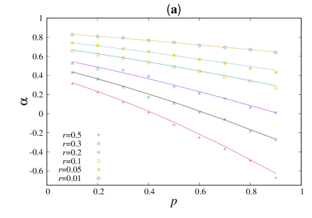
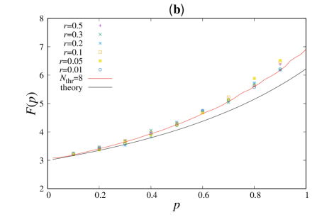
Figure 7: Testing the determination of $\alpha$ for the two-branch two-dimensional, two-branch model, using equation (8), and the $P_{k}$ derived from simulations with $N_{\rm thr}=8$. Left panel: there is satisfactory agreement between the empirical values of $\alpha$ and the values obtained from (8). Right panel: the data points collapse onto a plot of $F(p)\equiv(1-P_{1})/Q$, using values of $P_{k}$ derived from simulations (with $N_{\rm thr}=8$), compared with the values of $F(p)$ obtained from equations (29)-(33).

5.3 Two-dimensional model with four branches

In the case of the four-branch model, a theoretical calculation of the probabilities $P_{k}$ is considerably more difficult, although we can obtain formulae for $P_{1}$ and $P_{2}$ which are analogous to those obtained in the two-branch case, and find

$$P_{1}=1-7p+O(p^{2})$$ (35)

The calculation of the other $P_{k}$ is complicated, because once a site has branched from one site to its four neighbours, one has to consider transitions from the eight sites adjacent to the four newly occupied positions. Four of them can only reach one of the four new positions, but four of them could possibly reach two positions. We can, however, assert that $P_{3}=p+O(p^{2})$ and conclude that

$$\lim_{p\to 0}F(p)=\frac{3}{2}\ .$$ (36)

Numerical investigation of the probabilities $P_{k}$ for the four-way splitting model is difficult because, except when $p$ is small, the proportion of sites which do not undergo coalescence events is very small. Accordingly, we confined our numerical investigations to cases where $p<0.5$. Figures 8 and 9, illustrating investigations of the four-branch model, are similar to figures 6 and 7, but do not include theoretical predictions of $F(p)\equiv(1-P_{1})/Q$.

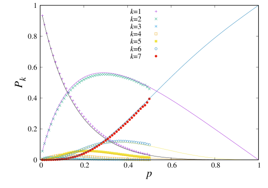
Figure 8: Numerical simulations of the functions $P_{k}(p)$, $k=1,\ldots,7$, for the two-dimensional, four-branch model. Two different numerical simulations are shown: one includes all sites (i.e. $N_{\rm thr}=0$, solid line), the other (points) imposes the requirement that the site has not experienced a coalescence in the preceding $N_{\rm thr}=6$ iterations.

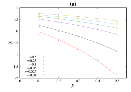
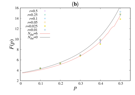
Figure 9: Testing the determination of $\alpha$ for the two-dimensional four-branch model, using (8), and the $P_{k}$ derived from simulations with $N_{\rm thr}=6$. Left panel: there is satisfactory agreement between the empirical values of $\alpha$ and the values obtained from (8). Right panel: the data points onto a plot of $F(p)\equiv(1-P_{1})/Q$, using values of $P_{k}$ derived from simulations (with $N_{\rm thr}=6$), compared with the values of $F(p)$ obtained from simulations which included all sites (i.e. setting $N_{\rm thr}=0$): there is a significant discrepancy as $p\to 1$.

6 Tests of exactness in the mass-conserving case

In the Introduction, we mentioned that, in one dimension, the case where $p_{0}=0$ appears to be exactly solvable. Here, we argue that the steady-state probability for occupying $N$ consecutive sites at step $j$ can be written as a product of independent probabilities at different sites. That is, if $s_{i}$ is the occupation of the $i^{\rm th}$ site, then we postulate the joint probability to be the product:

$$P_{N}(s_{1},s_{2},\ldots,s_{N})=\prod_{i=1}^{N}P_{1}(s_{i})=\prod_{i=1}^{N}\left[s_{i}f_{1}+(1-s_{i})(1-f_{1})\right]$$ (37)

where $f_{1}$ is the probability of occupation of a single site, given by (12). This result can be demonstrated by assuming that (37) holds at iteration $j$, and testing whether the joint probability given by Eq. 37 remains unchanged by the dynamics.

Because sites which are not adjacent to each other are not influenced by common sites at the previous iteration, non-adjacent pairs are obviously independent. In subsection 6.1 we investigate the joint probability $P_{2}(a,b)$ for two adjacent sites, and show that this factorises if we make an assumption about the relationship between the occupation probability, $f$, and the splitting probability, $p$. This relation need not necessarily be the same, as the function $f_{1}(p)$ given by (12), and we shall distinguish it by denoting this function by $\tilde{f}_{1}(p)$. The same approach is also used to determine functions $\tilde{f}_{2,2}(p)$ and $\tilde{f}_{2,4}(p)$ which would ensure that $P_{2}(a,b)=P_{1}(a)P_{1}(b)$ for the two-dimensional models. We show that $\tilde{f}_{1}(p)$ coincides with $f_{1}(p)$, implying that the one-dimensional model is exactly solvable, but that this does not hold for the two-dimensional cases.

We are also able to give an inductive demonstration of a more general result concerning the dynamics of the one-dimensional model: in section 6.2 we show that the boundary between an occupied and an unoccupied region fluctuates diffusively, while the occupation probabilities within the occupied region remain statistically independent.

6.1 Condition for factorisation

Consider two adjacent sites at step $j+1$. These were influenced by the configuration at step $j$ through their nearest neighbours. There is only one site, which will be referred to as the ‘key site’, which can influence both of the sites at step $j+1$ (see figure 10). So if we are seeking to establish whether sites are independent, this one site should receive special attention. This observation is also true in higher dimensions.

Figure 10: At iteration $j+1$, sites A an B are influenced by their nearest neighbours (illustrated here for the two-dimensional model) at iteration $j$. Correlations may result from the fact that both A and B are influenced by occupation of the ‘key site’, X.

Consider the influence of the key site, ${\rm X}$, upon its two nearest neighbours, ${\rm A}$ and ${\rm B}$. A ‘wetted bond’ connection may (probability $\tilde{P}_{1}$), or may not, (probability $\tilde{P}_{0}$), be made from the key site ${\rm X}$ to site ${\rm A}$. Let $a=0$ or $a=1$ indicate whether site ${\rm A}$ is (respectively) empty or occupied. Also let $P(a|0)$ be the probability that ${\rm A}$ becomes occupied at step $j+1$, given that no connection has been made to ${\rm A}$ from ${\rm X}$, and $P(a|1)$ be the probability that ${\rm A}$ is occupied if a connection is made from site ${\rm X}$. Clearly, $P(a|1)=a$, because ${\rm A}$ is definitely occupied if the connection is made, so that $P(1|1)=1$ and $P(0|1)=0$. With these definitions, we can write an expression for the probability of ${\rm A}$ being occupied at step $j+1$. The probability $P_{1}(a)$ of ${\rm A}$ being occupied has a contribution from a term where no connection is made from ${\rm X}$ to ${\rm A}$ (with probability $\tilde{P}_{0}$), multiplied by the probability for the independent event in which site ${\rm A}$ achieves occupancy $a$ by connections from its other neighbouring sites. Adding another term, representing events where ${\rm X}$ does connect to ${\rm A}$, we have

$$P_{1}(a)=P(a|0)\tilde{P}_{0}+P(a|1)\tilde{P}_{1}\ .$$ (38)

We shall need expressions for $\tilde{P}_{0}$ and $\tilde{P}_{1}$. These depend upon which version of the model we consider.

One-dimensional model

In the one-dimensional case, we assume that sites are occupied with probability $f$ at step $j$. So the probability of ${\rm X}$ being occupied and splitting is $fp$, and of ${\rm X}$ occupied and moving to the left without splitting is $f(1-p)/2$. Hence

$$\tilde{P}_{1}=\left(\frac{1+p}{2}\right)f\ ,\ \ \ \tilde{P}_{0}=1-\left(\frac{1+p}{2}\right)f\ .$$ (39)

Now consider the joint occupation probability of sites ${\rm A}$ and ${\rm B}$. Going from iteration $j$ to $j+1$, there is a probability $\tilde{P}_{00}$ that there is no transfer of occupation from ${\rm X}$ to either ${\rm A}$ or ${\rm B}$. The probability that ${\rm X}$ transfers to ${\rm B}$ and not ${\rm A}$ is $\tilde{P}_{01}$, and the probability to transfer to both sites is $\tilde{P}_{11}$. In the one-dimensional case, these probabilities are

$$\tilde{P}_{00}=1-f\ ,\ \ \ \tilde{P}_{01}=\frac{f}{2}(1-p)\ ,\ \ \ \tilde{P}_{11}=pf\ .$$ (40)

The joint probability at step $j+1$ for sites ${\rm A}$, ${\rm B}$ is

$$P_{2}(a,b) = P(a|0)P(b|0)\tilde{P}_{00}$$ (41)

$$+ \left[P(a|0)P(b|1)+P(a|1)P(b|0)\right]\tilde{P}_{01}$$

$$+ P(a|1)P(b|1)\tilde{P}_{11}\ .$$

Now use (41) and (38) to determine

$$P_{2}(a,b)-P_{1}(a)P_{1}(b) = P(a|0)P(b|0)\left[\tilde{P}_{00}-\tilde{P}_{0}^{2}\right]$$ (42)

$$+ \left[P(a|0)P(b|1)+P(a|1)P(b|0)\right]\left[\tilde{P}_{01}-\tilde{P}_{0}\tilde{P}_{1}\right]$$

$$+ P(a|1)P(b|1)\left[\tilde{P}_{11}-\tilde{P}_{1}^{2}\right]\ .$$

From (42), the occupations remain independent at step $j+1$ if all three of the following conditions are satisfied:

$$\tilde{P}_{00}=\tilde{P}_{0}^{2}\ ,\ \ \ \tilde{P}_{10}=\tilde{P}_{0}\tilde{P}_{1}\ ,\ \ \ \tilde{P}_{11}=\tilde{P}_{1}^{2}\ .$$ (43)

In the one-dimensional case, these conditions are

$$1-f = \left[1-\left(\frac{1+p}{2}\right)f\right]^{2}$$

$$(1-p)\frac{f}{2} = \left[1-\left(\frac{1+p}{2}\right)f\right]\left(\frac{1+p}{2}\right)f$$

$$pf = \left[\left(\frac{1+p}{2}\right)f\right]^{2}$$ (44)

These three equations all imply the same relationship between $f$ and $p$:

$$\tilde{f}_{1}(p)=\frac{4p}{(1+p)^{2}}$$ (45)

which is the same relationship between $f$ and $p$ as arises independently from the calculation of the filling fraction in the independent-site approximation, equation (12).

Note that this calculation didn’t require $P(a|0)$ or $P(b|1)$, only the probabilities $\tilde{P}_{0}$, $\tilde{P}_{00}$, $\tilde{P}_{01}$. It is, therefore, easily extended to the two-dimensional models that we considered.

Two-dimensional model

For the two-branch model

$$\tilde{P}_{00}=1-\frac{f}{2}\ ,\ \ \ \tilde{P}_{01}=\left(\frac{1-p}{4}\right)f\ ,\ \ \ \tilde{P}_{11}=p\frac{f}{2}$$

$${\bf two} - {\bf branch\ model}$$ (46)

$$\tilde{P}_{0}=1-\left(\frac{1+p}{4}\right)f\ ,\ \ \ \tilde{P}_{1}=\left(\frac{1+p}{4}\right)f\ .$$

In this case, equations (6.1) are satisfied by

$$\tilde{f}_{2,2}(p)=\frac{8p}{(1+p)^{2}}\ .$$ (47)

Similarly, for the four-branch model

$$\tilde{P}_{00}=1-\left(\frac{1+p}{2}\right)f\ ,\ \ \ \tilde{P}_{01}=\left(\frac{1-p}{4}\right)f\ ,\ \ \ \tilde{P}_{11}=pf$$

$${\bf four} - {\bf branch\ model}$$ (48)

$$\tilde{P}_{0}=1-\left(\frac{3p+1}{4}\right)f\ ,\ \ \ \tilde{P}_{1}=\left(\frac{3p+1}{4}\right)f\ .$$

In this case, equations (6.1) are satisfied by

$$\tilde{f}_{2,4}(p)=\frac{16p}{(3p+1)^{2}}\ .$$ (49)

In contrast with the one-dimensional model, in the two-dimensional cases the functions $\tilde{f}(p)$, which satisfy the factorisation condition, do not agree with the functions $f(p)$ which describe the occupation probability of the sites discussed in section 4. We conclude that the site occupations are not independent in the two-dimensional models.

6.2 One-dimensional case: finite intervals

We have shown that in the one-dimensional case, the independent-occupancy distribution is self-reproducing under iteration of the model in the mass-conserving case, $p_{0}=0$. We can also establish a stronger result on exactness of solutions of the one-dimensional case. Suppose that we know that at iteration $j$, the occupied region is bounded: it is known that sites $n_{-}$ and $n_{+}$ are occupied, and that everything to the left of $n_{-}$ and to the right of $n_{+}$ is empty. All the sites with a parity different from $j$ are empty. Let us assume that all of the sites $n$ with the same parity as $j$ satisfying $n_{-}<n<n_{+}$ are occupied with independently with probability $f_{1}$, given by (12). What can be said about the joint distribution of occupancy at the next ($j+1$) iteration?

The end values $n_{-}$ and $n_{+}$ both change by $\pm 1$, independently. At each end the boundary expands with probability $(1+p)/2$ or contracts with probability $(1-p)/2$. Let us assume that the shifts of the boundary have been determined, and consider the joint distribution of occupation of the other sites, conditional upon the new positions of the ends of the occupied interval.

We shall argue that if, at iteration $j$, the interior sites are independently occupied with probability $f_{1}$, then, they remain independently occupied with $f_{1}$ at iteration $j+1$. Because of the short range of influence of occupation probabilities at the next iteration, we can treat the two ends independently, and consider only a short interval in the vicinity of one end.

Figure 11: We consider configurations at the left-hand edge of the filled region. At iteration $j$ (blue sites), the configuration is $(0,1,a,b)$ (where $a\in\{0,1\}$ and $b\in\{0,1\}$ are variable). At iteration $j+1$ (red sites), the occupied region either expands (lower row, occupancy $(1,a^{\prime},b^{\prime})$) or else contracts (upper row, occupancy $(0,1,b^{\prime})$). We show that if $a,b$ are independent, with occupation probability $f_{1}=4p/(1+p)^{2}$, then $a^{\prime},b^{\prime}$ have the same property. Sites defined to be empty are shown as open circles, those defined filled are solid colour, and sites which are occupied with probability ${f_{1}}(p)$ are shaded.

We consider a sequence of four sites at iteration $j$, having the same parity as $j$. The first two of these have definite values $0$ and $1$, and the second two are variable, $a\in\{0,1\}$ and $b\in\{0,1\}$, as illustrated in figure 11. These four sites, $(0,1,a,b)$, influence the values of sites (of different parity) at the next iteration. We consider two cases: the case where the occupied region expands and the sequence at the next iteration is $(1,a^{\prime},b,)$, and also the contracting case where the occupations become $(0,1,b^{\prime})$.

In the contracting case, one calculates the probability of $b^{\prime}$, assuming that $a$ and $b$ are independent, with probability $f_{1}$ of being equal to $1$:

$${\rm Prob}(b^{\prime})=\sum_{(a,b)}P_{01|}(b^{\prime}|a,b)[f_{1}a+(1-f_{1})(1-a)][f_{1}b+(1-f_{1})(1-b)]$$ (50)

where $P_{01|}(b^{\prime}|a,b)$ is the conditional probability for obtaining $(0,1,b^{\prime})$ at iteration $j+1$ given $(0,1,a,b)$ at iteration $j$. Noting that the probability for a ‘contracting’ shift of the boundary is $(1-p)/2$, if the joint distribution of occupations is self-reproducing under iteration, we should expect that

$${\rm Prob}(b^{\prime})=\left(\frac{1-p}{2}\right)[f_{1}b^{\prime}+(1-f_{1})(1-b^{\prime})]\ .$$ (51)

Similarly, for the extending case, we can calculate the joint probability distribution of $(a^{\prime},b^{\prime})$:

$${\rm Prob}(a^{\prime},b^{\prime})=\sum_{(a,b)}P_{1|}(a^{\prime},b^{\prime}|a,b)[f_{1}a+(1-f_{1})(1-a)][f_{1}b+(1-f_{1})(1-b)]$$ (52)

where $P_{1|}(a^{\prime},b^{\prime}|a,b)$ is the conditional probability for obtaining $(1,a^{\prime},b^{\prime})$ at iteration $j+1$ given $(0,1,a,b)$ at iteration $j$. In this case, we expect

$${\rm Prob}(a^{\prime},b^{\prime})=\left(\frac{1+p}{2}\right)[f_{1}a^{\prime}+(1-f_{1})(1-a^{\prime})][f_{1}b^{\prime}+(1-f_{1})(1-b^{\prime})]\ .$$ (53)

There does not appear to be any transparent general expression for the conditional probabilities $P_{1|}(a,,b^{\prime}|a,b)$ and $P_{01|}(b^{\prime}|a,b)$, and we determined them on a case-by-case basis. They are tabulated in table 1. The first four rows determine $P_{1|}(a^{\prime},b^{\prime}|a,b)$, and the final two rows specify $P_{01|}(b^{\prime}|a,b)$.

Table 1: Conditional probabilities for reaching states $(1,a^{\prime},b^{\prime})$ or $(0,1,b^{\prime})$ (rows) from initial states $(0,1,a,b)$ (columns).

	(0,1,0,0)	(0,1,0,1)	(0,1,1,0)	(0,1,1,1)
(1,0,0)	$\frac{1-p}{2}$	$\left(\frac{1-p}{2}\right)^{2}$	$0$	$0$
(1,0,1)	$0$	$\left(\frac{1-p}{2}\right)\left(\frac{1+p}{2}\right)$	$\left(\frac{1-p}{2}\right)^{2}$	$\left(\frac{1-p}{2}\right)^{2}$
(1,1,0)	$p$	$\left(\frac{1-p}{2}\right)p$	$\left(\frac{1-p}{2}\right)\left(\frac{1+p}{2}\right)$	$\left(\frac{1-p}{2}\right)^{2}\left(\frac{1+p}{2}\right)$
(1,1,1)	$0$	$\left(\frac{1+p}{2}\right)p$	$2p\left(\frac{1-p}{2}\right)+p^{2}$	$1-\left(\frac{1-p}{2}\right)-\left(\frac{1-p}{2}\right)^{2}-\left(\frac{1-p}{2}\right)^{2}\left(\frac{1+p}{2}\right)$
(0,1,0)	$\left(\frac{1-p}{2}\right)$	$\left(\frac{1-p}{2}\right)^{2}$	$\left(\frac{1-p}{2}\right)^{2}$	$\left(\frac{1-p}{2}\right)^{2}$
(0,1,1)	$0$	$\left(\frac{1-p}{2}\right)\left(\frac{1+p}{2}\right)$	$\left(\frac{1-p}{2}\right)\left(\frac{1+p}{2}\right)$	$\left(\frac{1-p}{2}\right)\left[1-\left(\frac{1-p}{2}\right)^{2}\right]$

Using the expressions in table 1, we were able to verify that equations (51) and (50) are indeed equal, as are equations (53) and (52). We are not aware of any simpler route to this conclusion.

The same argument can be applied at the right-hand edge of the occupied region, so that the site occupations remain independent inside any occupied region, independent of how its boundaries fluctuate.

7 Relation to standard model for directed percolation

Here we discuss what happens, in one dimension, when $p_{0}\neq 0$. This includes the standard model for directed percolation as a special case, and we shall give emphasis to making connections with that problem. So in this section we will not consider the probability distribution of the flux $\phi$, but rather concentrate on the set of occupied sites. The model then has just two relevant parameters, $p_{0}$ and $p_{2}$.

When $p_{0}\neq 0$, there is a possibility for clusters of pathways to die out, so that the occupation fraction $f_{1}(p_{0},p_{2})$ is equal to zero when $p_{0}>p_{\rm c}$, where $p_{\rm c}$ is the percolation threshold. This percolation threshold is a function of $p_{2}$.

The standard directed bond-percolation problem is when the two bonds are filled independently with probability $p$, so that $p^{2}\equiv p_{2}$ and $(1-p)^{2}=p_{0}$. The standard directed percolation problem is therefore represented by the parametric line $p_{0}=(1-p)^{2}$, $p_{2}=p^{2}$ in the two-dimensional parameter space of our model.

In sub-section 7.1 we propose a bound on the percolation threshold, $p_{\rm c}(p_{2})$, and compare this with numerical estimates. Sub-section 7.2 presents some numerical investigations of the critical exponents of the model. We find that these appear to be identical to those of the standard directed percolation model, in accord with a hypothesis of Janssen ([5]) and Grassberger ([6]). In sub-section 7.3 we present numerical investigations of the PDF of the distribution of sizes of voids.

7.1 Phase diagram

The space of models is illustrated in figure 12. The allowed region of $p_{0}$, $p_{2}$ space is a triangle, $p_{0}\geq 0$, $p_{2}\geq 0$, $p_{0}+p_{2}\leq 1$. The line $p_{0}=0$ is exactly solvable for the equilibrium distribution as described by equation (12) and section 6. The standard directed bond-percolation problem with probability $p$ for bond occupation is the line $p_{0}=(1-p)^{2}$, $p_{2}=p^{2}$. We have plotted our numerical evaluation of the critical line, above which $f_{1}(p_{0},p_{2})=0$. The critical line crosses the line defining bond-directed percolation at $p=0.644\ldots$, as expected [12].

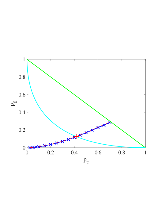
Figure 12: Parameter space of the one-dimensional model, showing the critical line for percolation transition (crosses). The conventional one-dimensional directed percolation problem, in which bonds are occupied independently with probability $p$, is represented parametrically by the line $p_{0}=(1-p)^{2}$, $p_{2}=p^{2}$, shown in blue. The red cross indicates the critical point for the standard directed bond-percolation model, at $p\approx 0.644$.

We were able to suggest an upper bound on the critical line using the following argument (which assumes that $p_{2}\ll 1$). We know that $p_{0}=0$ is exactly solvable, with those sites which are accessible on a given iteration are independently occupied with probability $f_{1}(0,p_{2})=4p_{2}/(1+p_{2})^{2}$. Because there are no correlations, the site occupation is a Poisson process. This expression implies that there are ‘voids’ between occupied sites which have a characteristic lengthscale $\langle L_{\rm v}\rangle$ which diverges as $p_{2}\to 0$. Assuming that the lattice spacing is unity, and noting that it is only every second site which is accessible, the mean length of the voids is

$$\langle L_{\rm v}\rangle\sim 1/(2p_{2})$$ (54)

when $p_{0}=0$. These voids have an exponential distribution of lengths.

A completely empty state is another possible solution. The dynamics of the system is described by the boundary between the empty state and an occupied region. This boundary is described by a single trajectory, and its treatment is more tractable than analysing the joint statistics of an occupied region. The path of the boundary is a random walk with a drift. In the limit where both $p_{0}$ and $p_{2}$ are small, we can characterise the motion of the boundary of the occupied region by a diffusion coefficient $D_{\rm b}$ and a drift velocity $v_{\rm b}$.

The diffusion coefficient is determined by writing $\langle\Delta x^{2}\rangle=2D\Delta t$, and noting that the displacement is unity (except in the rare cases where the trajectory terminates). There is a drift velocity into the empty region, which is determined by noting that when a trajectory splits, with probability $p_{2}$, the daughter trajectory on the void side become the new boundary. When $p_{0}=0$ the diffusion coefficient $D_{\rm b}$ and a drift velocity $v_{\rm b}$ (into the empty region) are.

$$D_{\rm b}=\frac{1}{2}\ ,\ \ \ v_{\rm b}=p_{2}\ .$$ (55)

Note that after coarse-graining the spatial and temporal scales, the edge of a void satisfies a stochastic differential equation of the form

$${\rm d}x=v_{\rm b}{\rm d}t+\sqrt{2D_{\rm b}}{\rm d}\eta(t)$$ (56)

where ${\rm d}\eta$ is a standard stochastic increment, satisfying $\langle{\rm d}\eta(t)\rangle=0$ and $\langle{\rm d}\eta(t){\rm d}\eta(t^{\prime})\rangle=\delta(t-t^{\prime})$. This is equivalent to a Fokker-Planck equation for the position of a void boundary:

$$\frac{\partial P}{\partial t}=-\frac{\partial}{\partial x}\left[v_{\rm b}P\right]+D_{\rm b}\frac{\partial^{2}P}{\partial x^{2}}\ .$$ (57)

A similar expression holds for the overall width of the void. Taking account of the fact that the void has two edges, both the drift velocity and the diffusion coefficient are doubled. The steady-state probability density for the distribution of large void sizes is then

$$P_{\rm v}(L)={\rm const.}\times\exp(-L/\langle L_{\rm v}\rangle)$$ (58)

where the steady state size scale for the large voids is $\langle L_{\rm v}\rangle=2D_{\rm b}/2v_{\rm b}\sim 1/2p_{2}$, which is in agreement with equation (54).

Consider what happens as $p_{0}$ is increased. When $p_{0}\neq 0$ there is a new mechanism which contributes to the drift velocity of the boundary. When a trail disappears, the boundary of the occupied region retreats by a distance $L_{1}$ equal to the length of the first void which is encountered. The velocity of the boundary is then

$$v_{\rm b}=p_{2}-p_{0}\langle L_{1}\rangle$$ (59)

which becomes negative at a critical value of $p_{0}$. The significance of this critical value is that for $p_{0}>p_{\rm c}$ the boundary of the occupied region retreats, until we are left with the empty configuration. We should expect that $\langle L_{1}\rangle$ increases when $p_{0}>0$, so that (when $p_{2}\ll 1$), $v_{\rm b}$ is bounded above:

$$v_{\rm b}\leq p_{2}-\frac{p_{0}}{2p_{2}}\ .$$ (60)

The critical value of $p_{0}$ occurs when $v_{\rm b}$ changes sign, so that

$$p_{\rm c}\leq 2p_{2}^{2}\ .$$ (61)

In figure 13 we plot $p_{0}/p_{2}^{2}$ for the transition line, as a function of $p_{2}$. The ratio is less than $2$, as predicted by equation (61). We do not have a theory for the form of this dependence.

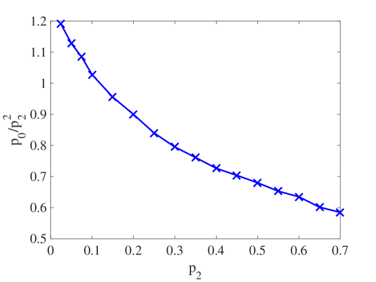
Figure 13: Ratio $p_{0}/p_{2}^{2}$ for transition line, showing consistency with equation (61).

Finally, we remark that our model is related to a model of directed percolation in which bonds are deleted with probability $1-p_{\rm bond}$, and sites are deleted with probability $1-p_{\rm site}$, as discussed in [16]. The parameters $p_{\rm bond}$ and $p_{\rm site}$ are related to our parameters as follows:

$$p_{0}=(1-p_{\rm site})+p_{\rm site}(1-p_{\rm bond})^{2}\ ,\ \ \ p_{2}=p_{\rm site}p_{\rm bond}^{2}\ .$$ (62)

This bond/site deletion model does not cover the whole parameter space of our model: the square $0\leq p_{\rm site}\leq 1$, $0\leq P_{\rm bond}\leq 1$ maps to the region to the right of the cyan line in figure 12. It can be verified that the region of the critical line of our model lying within this region is in agreement with the data in [16].

7.2 Critical exponents

The percolation process which we consider is a form of directed percolation. Grassberger [6] and Janssen [5] introduced a hypothesis that the directed percolation has universal critical exponents, and we expect that the transition in our model lies in this universality class. Thus we expect that $f_{1}(p_{0},p_{2})=0$ when $p_{0}>p_{\rm c}(p_{2})$, and that when $p_{\rm c}-p_{0}$ is small and positive we have

$$f_{1}(p_{0},p_{2})\sim|p_{\rm c}(p_{2})-p_{0}|^{\beta}\ .$$ (63)

where $\beta=0.276\ldots$ is the critical exponent for the order parameter of the directed percolation transition. Figure 14 presents evidence that the occupation fraction vanishes in accord with equation (63).

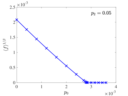
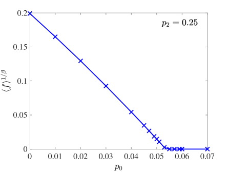
Figure 14: Occupied fraction approaching the percolation transition. The average fraction, to the power $1/\beta$, where $\beta$ is the exponent of directed percolation, shown as a function of $p_{0}$, reveals an approximately linear law. This is consistent with the expected behaviour $\langle f\rangle\propto(p_{c}(p_{2})-p_{0})^{\beta}$ when $p_{0}\rightarrow p_{c}(p_{2})$, see Eq. (63).

7.3 Void size distribution

We investigated the distribution of sizes of voids, $P_{\rm void}(n)$. The distribution, illustrated in figure 15 is highly distinctive: the is a ‘core’ region, in which $P_{\rm void}(n)$ has a rapid exponential decay, and a ‘tail’, which has a slower exponential decay, described by an exponent $\mu$:

$$P(n)\propto\exp(-\mu n)$$ (64)

The lengthscale associated with the slow decay diverges as the critical point is approached. (In figure 15 the void size $n$ is the number of potentially filled sites which are actually empty. Because sites with different parity from the iteration index are automatically empty, the void sizes disccused in sub-section 7.1 are approximately $2n$.)

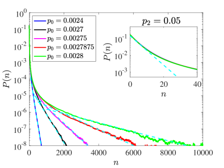
Figure 15: Void size distribution. The PDFs of the size distributions for $p_{2}=0.05$ (left) and $p_{2}=0.25$ (right) show broad tails, which can be approximately represented by an exponential form: $P(n)\propto\exp(-\mu n)$; as indicated by the dashed line in the figure. The exponent $\mu$ becoming very small when $p_{0}$ approaches the transition point. For small values of $n$, on the other hand, the distributions of $n$ are also exponential, consistent with equation (58): $P(n)\approx{f_{1}}^{n}$, with ${f_{1}}=4p_{2}/(1+p_{2}^{2})$, as indicated by the dashed line in the inset.

Figure 16 shows how values of the decay rate $\mu$ behaves as a function of the probability $p_{0}$, at the values of $p_{2}=0.05$, $0.1$ and $0.25$. In the spirit of directed percolation, one expects that the exponent $\mu\propto|p_{c}(p_{2})-p_{0}|^{\nu_{\perp}}$ when $p_{0}<p_{c}(p_{2})$. Since $\langle f\rangle\propto|p_{c}(p_{2})-p_{0}|^{\beta}$, Fig. 16 shows $\mu$ as a function of $\langle f\rangle^{\nu_{\perp}/\beta}$. Additionally, we divided the value of $\langle f\rangle^{\nu_{\perp}/\beta}$ by $p_{c}^{\nu_{\perp}}$, which reduces the various values to a unique curve. The dashed line shows a power law with a power $1$ (linear dependence), which closely agrees with the measured values of $\mu$ collapsed to a single curve.

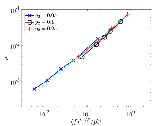
Figure 16: The decay rate $\mu$ of the void size distributions as a function of the normalised mean occupation fraction, $\langle f\rangle/p_{2}$, to the power $\nu_{\perp}/\beta$, where $\nu_{\perp}$ and $\beta$ are the classical directed percolation exponents [3]. The dashed line indicate a power $1$ corresponds to the directed percolation scaling, and describes approximately the numerical observations.

8 Conclusions, implications for elution

We introduced an alternative model for directed percolation which comes closer to addressing the questions originally posed by Broadbent and Hammersley [1]. Our model considers the distribution of fluxes $\phi$ through wetted bonds, and it has a flux-conserving regime, in which the total flux remains constant. Our model has similarities to the Scheidegger river model [18], which also involves addition of fluxes upon combining paths, and which also leads to a power-law distribution of fluxes [19]. The models differ as to the source of the flux: in our model the flux total flux is constant when $p_{0}=0$, whereas in the Scheidegger model new sources are added continuously.

We find that the distribution of fluxes $\phi$ is very broad, and in section 3 we showed that it has a power-law asymptote at small fluxes: $P(\phi)\sim\phi^{-\alpha}$. The exponent of this power law, $\alpha$, was found to vary continuously as a function of the parameters of the model. We found an exact equation for $\alpha$ (equation (8)) in terms of some probabilities $P_{k}$ (defined by (3)) which characterise the ‘wetting’ of the skeleton of bonds through which the fluxes flow.

In one dimension, the sites are independently occupied in the steady-state, implying that many quantities of interest, including the exponent $\alpha$, and the filling fraction for occupied sites, $f_{1}$, can be determined exactly.

In two dimensions, the independent-occupancy assumption gives a very good approximation for $\alpha$ and for the filling fractions, as shown in sections 4 and 5, but it is not exact. In section 6 we examined the conditions for the site occupations to remain independent under iteration. We found that these are only consistent with the predicted values of the filling fraction $f$ in the one-dimensional case.

In the case where the paths can terminate, the model is no longer flux conserving, and we find that the distribution of wetted bonds has a percolation transition. In section 7 we showed that, in the one-dimensional case, the critical exponents are in agreement with those of the standard directed percolation model. We also investigated the distribution of void sizes.

The long-tailed distribution of fluxes is expected to have practical consequences. Consider the following model for an elution process. For definiteness we discuss a solute being washed out of a solid substrate by a liquid. Leaching of a salt from a permeable rock or from land reclaimed from the sea would be a concrete example. We assume that the solid medium is permeated by randomly arranged narrow channels, but that on a large scale it appears homogeneous. We shall assume that the fluid is being forced through the medium, by gravity, or a pressure difference (or both).

If the solid contains solute with a concentration $c$ (defined as mass per unit volume), this will come into equilibrium with the salt dissolved in the liquid phase at a concentration $Kc$, where $K$ is a partition coefficient. If the liquid is flowing in very narrow channels, we can assume that the solute equilibrates between the solid and liquid phases, so that the concentration in the fluid flowing through the pore is also $Kc$. The rate at which solute is removed from the medium by flow through the pore is therefore $\dot{m}=Kc\phi$, where $\phi$ is the volume flux through the pore. The concentration is proportional to the amount of solute remaining in the solid phase, so that we expect that the concentration in the runoff through the pore reduces exponentially as a function of time. We therefore expect that the rate of loss of solute from a single pore is

$$\dot{m}=Kc(0)\phi\exp[-\nu\phi t]$$ (65)

where $\nu$ is dependent upon the geometry of the pore and the coefficient of solubility in the liquid and solid phases.

In the case of perfusion through a random medium, the liquid may follow many different channels (labelled by an index $i$), with very different volume fluxes $\phi_{i}$ in different channels. In this case, the total rate of solute out of the medium is

$$\dot{M}(t)=\sum_{i}\dot{m}_{i}(t)=Kc(0)\sum_{i}\phi_{i}\exp(-\nu_{i}\phi_{i}t)\ .$$ (66)

We shall argue that the predominant factor determining the rate of elution at long times is the existence of pores which carry very low fluxes. For this reason we adopt the simplifying assumption that the coefficients $\nu_{i}$ are the same for all of the pores. If the probability density function of $\phi$ is $P(\phi)$, and the density of pores carrying fluid is $\rho$, then the time-dependence of the eluted flux from a surface of area $A$ is

$$\dot{M}(t) = K\rho Ac(0)\int_{0}^{\infty}{\rm d}\phi\ P(\phi)\phi\exp(-\nu\phi t)$$ (67)

$$= -K\rho Ac(0)\frac{{\rm d}\bar{P}}{{\rm d}s}\bigg{|}_{\nu t}$$

where $\bar{P}(s)$ is the Laplace transform of $P(\phi)$. Determining the long-time behaviour depends upon the distribution of $\phi$ in the limit as $\phi\to 0$. We have argued that this has a power-law behaviour for a wide range of models. This indicates that there are many channels which have an extremely small flux, corresponding to a slow elution of the solute. Using (67), this corresponds to a power-law decay of the eluted solute flux:

$$\dot{M}(t) \sim c(0)A\rho\int_{0}^{\infty}{\rm d}\phi\ \phi^{1-\alpha}\exp(-\nu\phi t)$$ (68)

$$= \Gamma(2-\alpha)c(0)A\rho(\nu t)^{\alpha-2}\ .$$

It is noteworthy that, due to the power-law distribution of the flux $\phi$, despite the fact that the elution from each channel decreases exponentially as a function of time, the overall rate of elution has a much slower, power-law, decay. This is a consequence of the log-time behaviour being dominated by the channels with the smallest flux.

Acknowledgements. The authors are grateful to Robert Ziff for pointing out reference [16], and its relevance to our system, as expressed by equation (62). The project was initiated at the Kavli Institute for Theoretical Physics for support, where this research was supported in part by the National Science Foundation under Grant No. PHY11-25915.

References

References

- [1] S. R. Broadbent and J. M. Hammersley, Percolation processes: I. Crystals and mazes, Math. Proc. Cambridge Phil. Soc., 53, 629-41, (1957).
- [2] D. Stauffer and A. Aharony, Introduction To Percolation Theory, 2nd ed., Taylor & Francis, ISBN 9780748402533, (1992).
- [3] H. Hinrichsen, Non-equilibrium critical phenomena and phase transitions into absorbing states, Adv. Phys., 49, 815–958, (2000).
- [4] P. Grassberger and A. de la Torre, Reggeon field theory (Schlögl’s first model) on a lattice; Monte Carlo calculations of critical behaviour, Ann. Phys. (N.Y.), 122, 373–96, (1979).
- [5] H. K. Janssen, On the nonequilibrium phase transition in reaction-diffusion systems with an absorbing stationary state, Z. Phys. B, 42, 151–154, (1981).
- [6] P. Grassberger, On phase transitions in Schlögl’s second model, Z. Phys. B, 47, 365–374, (1982).
- [7] B. M. Arora, M. Barma, D. Dhar and M. K. Phani, Conductivity of a two-dimensional random diode-insulator network, J. Phys. C: Solid State Phys., 16, 2913-21, (1983).
- [8] S. Redner, Percolation and Conduction in Random Resistor-Diode Networks, in Percolation Structures and Processes, Annals of the Israel Physical Society, issue 5, eds. G. Deutscher, R. Zallen, J. Adler, A. Hilger, ISSN 0309-8710, (1983).
- [9] W. Kinzel, Phase transitions in cellular automata, Z. Phys. B, 58, 229-244 (1985).
- [10] E. Domany and W. Kinzel, Equivalence of cellular automata to Ising models and directed percolation, Phys. Rev. Lett., 53, 311-314 (1984).
- [11] R. M. Ziff, E. Gulari, and Y. Barshad, Kinetic phase transitions in an irreversible surface-reaction model, Phys. Rev. Lett., 56, 2553-6, (1986).
- [12] R. J. Baxter and A. J. Guttmann, Series expansion of the percolation probability for the directed square lattice, J. Phys. A: Math. Gen., 21 3193, (1988).
- [13] H. Takayasu and A. Yu. Tretyakov, Extinction, Survival, and Dynamical Phase Transition of Branching Annihilating Random Walk, Phys. Rev.Lett., 68, 3060-3, (1992).
- [14] G. Huber, M. H. Jensen and K. Sneppen, Distributions of self-interactions and voids in (1+1)-dimensional directed percolation, Phys. Rev. E, 52, R2133, (1995).
- [15] P. Grassberger, Are damage spreading transitions generically in the universality class of directed percolation?, J. Stat. Phys., 79, 13–23, (1995).
- [16] A. Yu. Tretyakov and N. Inui, Critical behaviour for mixed site-bond directed percolation, J. Phys. A: Math. Gen., 28, 3985-90, (1995).
- [17] K. Kawagoe, G. Huber, M. Pradas, M. Wilkinson, A. Pumir, and E. Ben-Naim, Aggregation-Fragmentation-Diffusion Model for Trail Dynamics, Phys. Rev. E, 96, 012142, (2017).
- [18] A. E. Scheidegger, International Association of Scientific Hydrology Bulletin, 12, (1967).
- [19] G. Huber, Scheidegger’s rivers, Takayasu’s aggregates and continued fractions, Physica A, 170, 463-470, (1991).
- [20] O. Narayan and D. S. Fisher, Nonlinear fluid flow in random media: Critical phenomena near threshold, Phys. Rev. B, 49, 9469-9502, (1993).
- [21] J. Watson and D. S. Fisher, Collective particle flow through random media, Phys. Rev. B, 54, 938-54, (1996).