DARTH: Holistic Test-time Adaptation for Multiple Object Tracking

Abstract

Multiple object tracking (MOT) is a fundamental component of perception systems for autonomous driving, and its robustness to unseen conditions is a requirement to avoid life-critical failures. Despite the urge of safety in driving systems, no solution to the MOT adaptation problem to domain shift in test-time conditions has ever been proposed. However, the nature of a MOT system is manifold - requiring object detection and instance association - and adapting all its components is non-trivial. In this paper, we analyze the effect of domain shift on appearance-based trackers, and introduce DARTH, a holistic test-time adaptation framework for MOT. We propose a detection consistency formulation to adapt object detection in a self-supervised fashion, while adapting the instance appearance representations via our novel patch contrastive loss. We evaluate our method on a variety of domain shifts - including sim-to-real, outdoor-to-indoor, indoor-to-outdoor - and substantially improve the source model performance on all metrics. Code: https://github.com/mattiasegu/darth.

1 Introduction

mot represents a cornerstone of modern perception systems for challenging computer vision applications, such as autonomous driving [17], video surveillance [16], behavior analysis [28], and augmented reality [48]. Laying the ground for safety-critical downstream perception and planning tasks - e.g. obstacle avoidance, motion estimation, prediction of vehicles and pedestrians intentions, and the consequent path planning - the robustness of mot to diverse conditions is of uttermost importance.

However, domain shift [30] could result in life-threatening failures of mot pipelines, due to the perception system’s inability to understand previously unseen environments and provide meaningful signals for downstream planning. To the best of our knowledge, despite the urge of addressing domain adaptation for mot to enable safer driving and video analysis, no solution has ever been proposed.

		$t=\hat{t}$	$t=\hat{t}+k$
Source
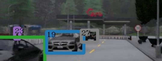
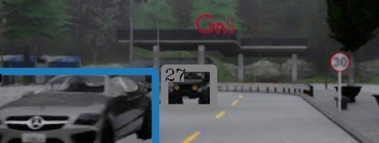
Target	No Adap.
	DARTH

Figure 1: We illustrate the effect of domain shift on mot, and how our test-time adaptation technique (DARTH) counteracts it. The top row shows the in-domain performance of a model trained on the synthetic dataset SHIFT [62] (Source); the same model (No Adap.) suffers from domain shift when deployed on the real-world BDD100K [72] (Target); the bottom row shows the benefits of DARTH. Each row shows two frames spaced by $k\mkern 1.5mu{=}\mkern 1.5mu\text{2}$ seconds; boxes of the same color correspond to the same tracking ID.

This paper analyzes the effect of domain shift on mot, and proposes a test-time adaptation solution to counteract it. We focus on appearance-based tracking, which shows state-of-the-art performance across a variety of datasets [21], outperforms motion-based trackers in complex scenarios - i.e. BDD100K [72] - and complements motion cues for superior tracking performance [77]. Since appearance-based trackers [33, 68, 1, 47] associate detections through time based on the similarity of their learnable appearance embeddings, domain shift threatens the performance of both their detection and instance association stages (Table 1).

tta offers a practical solution to domain shift by adapting a pre-trained model to any unlabeled target domain in absence of the original source domain. However, current tta techniques are tailored to classification tasks [65, 8, 66, 42] or require altering the source training procedure [63, 37, 44], and they have been shown to struggle in complex scenarios [37]. Consequently, the development of tta solutions for mot is non-trivial. While recent work further investigates tta for object detection [35, 59], solving tta for detection is not sufficient to recover mot systems (see SFOD [35] in Table 5), as instance association plays an equally crucial role in tracking.

To this end, we introduce a holistic test-time adaptation framework that addresses the manifold nature of mot (Figure 2). We propose a detection consistency formulation to adapt object detection in a self-supervised fashion and enforce its robustness to photometric changes, since tracking benefits from consistency of detection results in adjacent frames. Moreover, we adapt instance association and learn meaningful instance appearance representations on the target domain by introducing a patch contrastive loss, which enforces self-matching of the appearance of detected instances under differently augmented views of the same image. Finally, we update the teacher as an ema of the student model to benefit from the adapted student representations and gradually improve the detection targets for our consistency loss.

We name DARTH our test-time Domain Adaptation method for Recovering multiple object Tracking Holistically. To the best of our knowledge, our proposal is the first solution to the domain adaptation problem for mot. We evaluate DARTH on a variety of domain shifts across the driving datasets SHIFT [62] and BDD100K [72], and the pedestrian datasets MOT17 [41] and DanceTrack [60], showing substantial improvements over the source model performance on all the evaluated metrics and settings.

We summarize our contributions: (i) we study the domain shift problem for mot and introduce the first test-time adaptation solution; (ii) we propose a detection consistency formulation to adapt object detection and enforce its consistency to photometric changes; (iii) we introduce a patch contrastive approach to adapt the appearance representations for better data association.

Source	Target	DetA	MOTA	HOTA	IDF1	AssA
	[HTML]E0FCE0SHIFT	[HTML]E0FCE046.9	[HTML]E0FCE048.4	[HTML]E0FCE055.2	[HTML]E0FCE060.6	[HTML]E0FCE065.8
SHIFT	BDD100K	12.0	-66.4	17.3	18.5	28.9
	[HTML]E0FCE0MOT17	[HTML]E0FCE057.2	[HTML]E0FCE068.2	[HTML]E0FCE057.1	[HTML]E0FCE068.5	[HTML]E0FCE057.4
	DanceTrack	52.4	57.2	21.5	19.5	9.0
MOT17	BDD100K	23.2	10.5	27.2	33.3	32.4
	[HTML]E0FCE0MOT17	[HTML]E0FCE059.8	[HTML]E0FCE071.7	[HTML]E0FCE059.7	[HTML]E0FCE071.6	[HTML]E0FCE058.7
	DanceTrack	61.8	74.0	31.1	29.6	15.8
MOT17 (+CH)	BDD100K	32.4	28.3	33.7	41.7	35.4
	[HTML]E0FCE0DanceTrack	[HTML]E0FCE068.5	[HTML]E0FCE079.2	[HTML]E0FCE043.5	[HTML]E0FCE042.3	[HTML]E0FCE028.0
	MOT17	24.7	23.3	32.6	35.4	43.5
DanceTrack	BDD100K	9.3	-16.0	14.1	12.3	21.8
	[HTML]E0FCE0BDD100K	[HTML]E0FCE036.5	[HTML]E0FCE014.2	[HTML]E0FCE039.6	[HTML]E0FCE048.2	[HTML]E0FCE043.3
	MOT17	28.6	31.4	36.0	43.5	45.8
BDD100K	DanceTrack	41.9	41.6	18.0	17.0	7.9

Table 1: Domain shift in mot. We assess the impact of domain shift on the performance of a QDTrack model based on Faster R-CNN with a ResNet-50 backbone. In green the performance on the source domain. The ${\text{SHIFT}\rightarrow\text{BDD100K}}$ metrics are averaged across all object categories; only the pedestrian category is considered for all other experiments. CH: CrowdHuman.

2 Related Work

Multiple Object Tracking. Tracking-by-detection, i.e. detecting objects in individual frames of a video and associating them over time, is the dominant paradigm in mot. Motion- [3, 4, 20, 6, 77], appearance- [33, 68, 1, 47], and query-based [40, 61, 73] trackers are commonly used to associate the instances detected by an object detector. In this work, we focus on domain adaptation of appearance-based trackers, building on the state-of-the-art QDTrack [47, 21]. QDTrack introduces a quasi-dense paradigm for learning appearance representations, exceeding the association ability of motion- and query-based trackers. Moreover, appearance provides a complementary cue to motion [77]. Nevertheless, Table 1 shows that domain shift threatens both object detection and the learned appearance representations of QDTrack, negatively affecting instance association in mot. Previous work partially investigated mot under diverse conditions [22] and limited labels [38]. Our paper provides the first comprehensive analysis of domain shift in mot, and introduces an holistic framework to counteract its effect on the object detection and data association stages of appearance-based trackers.

Test-time Adaptation. Differently from uda [67], which assumes the availability of target samples when training on the source domain, test-time adaptation aims at adapting a source pre-trained model on any unlabeled target domain in absence of the original source domain. A popular approach to tta consists in learning, together with the main task, an auxiliary task with easy self-supervision on the target domain, e.g. geometric transformations prediction [15, 23, 63], colorizing images [75, 32], solving jigsaw puzzles [44]. However, such techniques require to alter the training procedure on the source domain to also learn the auxiliary task. Recent approaches allow instead to perform fully test-time adaptation without altering the source training. [55, 43, 42, 56] show the benefits of simply tuning on the target domain the batch normalization statistics of a frozen model. Tent [65] minimizes the output self-entropy on the target domain to learn the shift and scale parameters of the bn layers while using the batch statistics. Such techniques do not finetune the task-specific head while altering its expected input distribution, deteriorating the model performance under severe distribution shifts [37]. AdaContrast [8] and CoTTA [66] instead enforce prediction consistency under augmented views, learning global representations on the target domain for image classification. In contrast, the combination of our detection consistency formulation and our patch contrastive learning enables DARTH to simultaneously learn global and local representations on the target domain, while adapting respectively the task-specific detection and appearance heads.

Domain Adaptation for Object Detection. Object detection [50, 49] plays a key role in tracking-by-detection. Several works [45] focus on the unsupervised domain adaptation problem for object detection, adopting traditional techniques such as adversarial feature learning [10, 53, 27, 58], image-to-image translation [74, 7, 51], pseudo-label self-training [29, 31, 52], and mean-teacher training [5, 14]. However, such techniques require the availability of the labeled source domain. A more practical test-time adaptation solution [34] shows promising results by self-training with high-confidence pseudo-labels, though only on arbitrary and mild domain discrepancies such as Cityscapes [12] to Foggy Cityscapes [54] or to BDD100K [72] daytime. Similarly, normalization perturbation [18, 19] trains object detectors invariant to domain shift. Finally, object detection adaptation techniques do not seamlessly extend to mot adaptation, since the latter requires a further data association stage and detection consistency through time.

3 DARTH

We here introduce DARTH, our test-time adaptation method for mot. We first introduce the tta setting (Section 3.1) and give an overview of DARTH (Section 3.2). We further detail our patch contrastive learning and detection consistency formulation in Sections 3.3 and 3.4.

3.1 Test-time Adaptation for mot

Test-time adaptation addresses the problem of adapting a model previously trained on a source domain ${\mathcal{S}=\{(x_{s}^{i},y_{s}^{i},)\}_{i=1}^{N_{s}}}$ to an unlabeled target domain ${\mathcal{T}=\{x_{t}^{i}\}_{i=1}^{N_{t}}}$, without accessing the source domain.

In this work, we tackle the tta problem for mot, building on the state-of-the-art appearance-based tracker QDTrack [47]. Following the tracking-by-detection paradigm, modern mot methods [47, 6, 77] rely on a detection stage and a data association stage. QDTrack extends a Faster R-CNN [50] detector with an additional embedding head, and learns appearance similarity via a multi-positive contrastive loss that enforces discriminative instance representations. Under domain shift, all the components of the tracking pipeline fail, with significant performance drops on both detection and association metrics (Table 1).

3.2 Overview

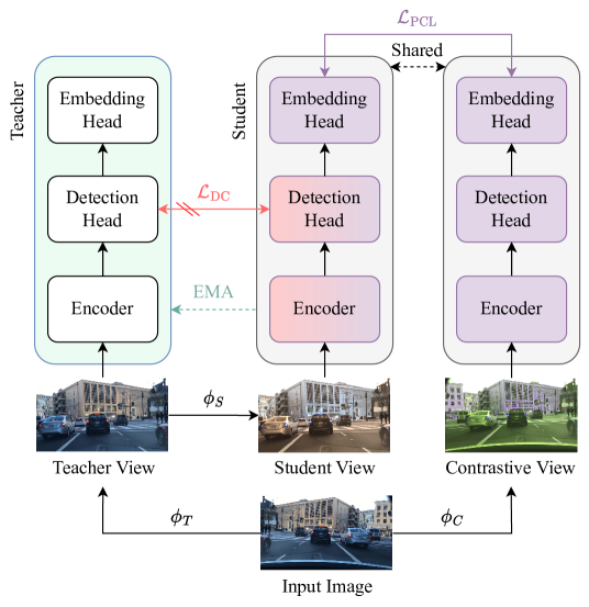
Figure 2: Schematic representation on the target domain of DARTH, our test-time adaptation method for mot. Our patch contrastive loss $\mathcal{L}_{\text{PCL}}$ between the siamese student’s instance embeddings adapts instance association. Our detection consistency loss $\mathcal{L}_{\text{DC}}$ enforces consistency to photometric changes. The EMA updates to the teacher gradually improve the detection targets for our consistency loss. $\phi_{T}$, $\phi_{S}$, and $\phi_{C}$ are the image transformations described in Section 3.2. ‘\\’ = stop gradient.

mot systems are composed of an object detection and a data association stage, tightly-coupled with each other. Adapting the one does not necessarily have a positive effect on the other (Table 6). To address this problem, we introduce DARTH, a holistic tta framework that addresses the manifold nature of mot by emphasizing the importance of the whole and the interdependence of its parts.

Architecture. DARTH relies on a teacher model and a siamese student (Figure 2). Given a set of QDTrack weights $\hat{\theta}$ trained on the source domain following [47], the student network is defined by a set of weights ${\theta\coloneqq\hat{\theta}}$. The teacher shares the same architecture with the student and its weights $\xi$ are initialized from the student weights $\hat{\theta}$ and updated as an ema of the student parameters $\theta$ during adaptation: ${\xi\leftarrow\tau\xi+(1-\tau)\theta}$. $\tau$ is the momentum of the update. The momentum teacher provides the targets to our detection consistency loss (Section 3.4) between teacher and student detection outputs under two differently augmented versions (views) of the same image. The siamese student enables learning discriminative appearance representations via our patch contrastive loss (Section 3.3) between the detections of two views of the same image. At inference time, we use our DARTH-adapted model to detect objects and extract instance embeddings, and apply the standard QDTrack inference strategy described in [47] to track objects in a video.

Views Definition. Figure 2 illustrates a schematic view of our framework and of the generation process of the different input views. Given an input image $x$, we apply a geometric augmentation $\phi_{T}$ to generate the teacher view $x_{T}$, and apply a subsequent photometric augmentation $\phi_{S}$ to produce the student view $x_{S}$. We generate $x_{S}$ from $x_{T}$ to satisfy the assumption of geometric alignment of teacher and student views in our detection consistency loss. The contrastive view $x_{C}$ used in the siamese pair is independently generated by applying a sequence $\phi_{C}$ of geometric and photometric augmentations on the original input image. We ablate on the impact of different augmentation strategies in Section 4.3. Details on the choice and parameters of geometric and photometric augmentations are in the Appendix.

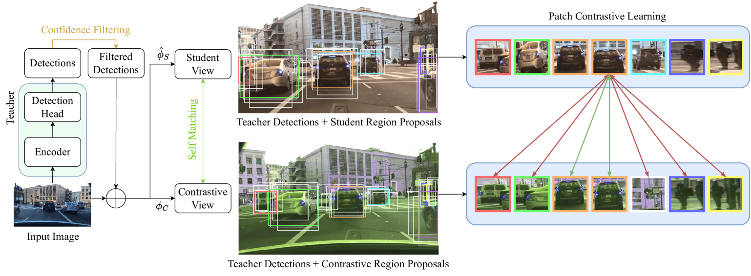
Figure 3: We here illustrate our novel patch contrastive formulation (Section 3.3). First, we identify object regions by applying the teacher detector on the input image and filtering the detections based on their confidence. We then apply on the input image and detected bounding boxes the transformations $\hat{\phi}_{S}$ and $\phi_{C}$ to generate the student and contrastive view, deriving association pseudo-labels by considering a match as positive when proposed regions (white) on different views match to a same teacher detection (identified by the same color across both views). Finally, we apply a multi-positive patch contrastive loss on the projections of the proposed regions obtained via the student embedding head. We here show an example of positive (green) and negative (red) matches for one of the student-view proposed regions.

3.3 Patch Contrastive Learning

To adapt the data association stage and learn discriminative appearance representations on the target domain, we introduce a novel pcl formulation, whose functioning is illustrated in Figure 3.

Localizing Objects. The goal of this step is identifying on the two views object regions over which learning instance-discriminative appearance representations, and filter out false positive detections. Given an image $x$ from the target domain $\mathcal{T}$ and the set of $K$ detections $D\mkern 1.5mu{=}\mkern 1.5mu\{d_{i}\}_{i=1}^{K}$ extracted by the teacher detector, we filter the detections by retaining only those with confidence higher than a threshold $\gamma$, i.e. ${\hat{D}\mkern 1.5mu{=}\mkern 1.5mu\{d\in D|\text{conf}(d)\geq\gamma\}}$. We then generate the student and contrastive views $x_{S}$ and $x_{C}$ by respectively applying on $x$ the image transformations $\hat{\phi}_{S}=\phi_{T}\circ\phi_{S}$ and $\phi_{C}$, and coherently warping the detections to $\hat{D}_{S}$ and $\hat{D}_{T}$.

Quasi-dense Formulation. We then phrase the patch contrastive learning problem as quasi-dense self-matching of the contrastive-view roi $R_{C}$ - i.e. Faster R-CNN region proposals - to the student-view proposals $R_{S}$. Since the student- and contrastive-view detections $\hat{D}_{S}$ and $\hat{D}_{C}$ are generated by augmenting the same teacher detections $\hat{D}$, instance correspondences between $x_{S}$ and $x_{C}$ are known in advance. In particular, we output image-level features through the student encoder, use the rpn to generate roi from the two images and RoI Align [25] to pool their feature maps at different levels in the fpn [36] according to their scales. For each roi we extract deeper appearance features via the additional embedding head. A roi in a view $x_{i}$ is considered a positive match to a detection $\hat{D}_{i}$ on the same view if they have iou higher than $\alpha_{1}=0.7$, negative if lower than $\alpha_{2}=0.3$. The matching of roi under the two views $x_{S}$ and $x_{C}$ is positive if both regions are associated to the same teacher detection $\hat{D}$; negative otherwise.

Patch Contrastive Learning. Assuming that $V$ positive roi are proposed on the student view $x_{S}$ as training samples and $K$ roi on the contrastive view $x_{C}$ as contrastive targets, we use the non-parametric softmax [70, 64] with cross-entropy to optimize the appearance embeddings of each training sample. We here only show the loss for one training sample, but average it over all of them:

$$\mathcal{L}_{\text{embed}} =-\sum_{\textbf{k}^{+}}\text{log}\frac{\text{exp}(\textbf{v}\cdot\textbf{k}^{+})}{\text{exp}(\textbf{v}\cdot\textbf{k}^{+})+\sum_{\textbf{k}^{-}}\text{exp}(\textbf{v}\cdot\textbf{k}^{-})},$$ (1)

where v are roi embeddings on $x_{S}$, and $\textbf{k}^{+}$, $\textbf{k}^{-}$ are their positive and negative targets on $x_{C}$.

Analogously to [47], we reformulate Eq. (1) to avoid considering each negative target $\textbf{k}^{-}$ multiple times per training sample v, while only once the positive one $\textbf{k}^{+}$:

$$\mathcal{L}_{\text{embed}}=\text{log}[1+\sum_{\textbf{k}^{+}}\sum_{\textbf{k}^{-}}\text{exp}(\textbf{v}\cdot\textbf{k}^{-}-\textbf{v}\cdot\textbf{k}^{+})].$$ (2)

We further adopt an L2 auxiliary loss to constrain the logit magnitude and cosine similarity:

$$\mathcal{L}_{\text{aux}}=\left(\frac{\textbf{v}\cdot\textbf{k}}{||\textbf{v}||\cdot||\textbf{k}||}-\mathbbm{1}_{\{\textbf{k}\in\left\{\textbf{k}^{+}\}\right\}}\right)^{2},$$ (3)

where $\mathbbm{1}$ is the indicator function and k an roi embedding such that $\textbf{k}\in\{\textbf{k}^{-}\}\cup\{\textbf{k}^{+}\}$. We calculate the auxiliary loss over all positive pairs and three times more negative pairs.

3.4 Detection Consistency

While our pcl adapts the local appearance representations to the target domain and improves instance association, not imposing any additional constraint might let the global image features deviate from the distribution expected by the detection head and damage the overall performance (Table 6). Inspired by self-supervised representation learning for image classification [24], we introduce a dc loss between predictions of the teacher and student detection heads under different image augmentations to adapt object detection to the target domain, while ema updates to the teacher model gradually incorporate the improved student representations and enable better targets for the consistency loss.

A by-product of our self-consistency to different augmentations is fostering better global representations on the target domain, complementary to the local representations learned via our pcl. Moreover, tracking-by-detection is negatively affected by flickering of detections through time, and domain shift exacerbates this issue. We find that enforcing detection consistency under different photometric augmentations stabilizes detection outputs in adjacent frames, significantly improving MOTA [2] (Table 7).

In particular, our detection consistency loss is composed of an RPN- and an RoI-consistency component applied on the RPN and roi heads in Faster R-CNN. Notice that our method applies to other two-stage detectors, and extends to one-stage detectors by ignoring the RPN consistency loss. We now present the details of our method.

Views Definition. We contextualize our choices on the views generation protocol (Section 3.2). We generate the teacher image $x_{T}$ by applying a geometric augmentation $\phi_{T}$ on the input image $x$. Since the teacher predictions should provide high-quality targets for the student, we do not further corrupt $x_{T}$ with photometric augmentations. Moreover, our dc loss requires geometric alignment of $x_{T}$ and $x_{S}$. We thus generate $x_{S}$ by applying a photometric augmentation $\phi_{S}$ on the teacher view $x_{T}$ to satisfy geometric alignment and allow consistency under photometric changes.

RPN Consistency. We implement RPN consistency as an $\mathcal{L}_{2}$ loss between the teacher $\xi$ and student $\theta$ RPN regression - i.e. displacement w.r.t. anchors - and classification outputs on $x_{T}$ and $x_{S}$. Inspired by model compression [9], we control the regression consistency by a threshold $\epsilon=0.1$ on the difference between the teacher and student classification outputs. We define the RPN consistency loss as:

$$\mathcal{L}^{\text{\ac{rpn}}}_{\text{DC}}=\frac{1}{N}\sum\left(\begin{Vmatrix}s_{\xi}-s_{\theta}\end{Vmatrix}_{2}^{2}+\mathbbm{1}_{\{s_{\xi}>s_{\theta}+\epsilon\}}\begin{Vmatrix}r_{\xi}-r_{\theta}\end{Vmatrix}_{2}^{2}\right),$$ (4)

where $\mathbbm{1}$ is the indicator function, $N$ the number of anchors, $s$ the rpn classification logits, $r$ the rpn regression output.

roi Consistency. We feed the teacher proposals into the student roi head and enforce an $\mathcal{L}_{2}$ consistency loss with the final teacher regression - i.e. displacement w.r.t. region proposals - and classification outputs. For each roi classification output - the logits $p$ - we subtract the mean over the class dimension to get the zero-mean classification result, $\tilde{p}$. Given $K$ sampled roi, $C$ classes including background, and the bounding box regression result $t$, we derive the roi consistency loss as:

$$\mathcal{L}^{\text{\ac{roi}}}_{\text{DC}}=\frac{1}{K\cdot C}\sum\left(\begin{Vmatrix}\tilde{p}_{\xi}-\tilde{p}_{\theta}\end{Vmatrix}_{2}^{2}+\begin{Vmatrix}t_{\xi}-t_{\theta}\end{Vmatrix}_{2}^{2}\right)$$ (5)

3.5 Total Loss

The entire framework is jointly optimized under a weighted sum of the individual losses:

$$\mathcal{L} =\gamma_{1}\mathcal{L}_{\text{embed}}+\gamma_{2}\mathcal{L}_{\text{aux}}+\gamma_{3}\mathcal{L}^{\text{\ac{rpn}}}_{\text{DC}}+\gamma_{4}\mathcal{L}^{\text{\ac{roi}}}_{\text{DC}}$$ (6)

$$=\mathcal{L}_{\text{PCL}}+\gamma_{3}\mathcal{L}^{\text{\ac{rpn}}}_{\text{DC}}+\gamma_{4}\mathcal{L}^{\text{\ac{roi}}}_{\text{DC}},$$ (7)

where $\gamma_{1}$, $\gamma_{2}$, $\gamma_{3}$ and $\gamma_{4}$ are set to 0.25, 1.0, 1.0 and 1.0. $\mathcal{L}_{\text{PCL}}=\gamma_{1}\mathcal{L}_{\text{embed}}+\gamma_{2}\mathcal{L}_{\text{aux}}$ is the total pcl loss.

In Section 4.3 we ablate on the need for each individual component, showing the importance of a holistic adaptation solution for mot that emphasizes the importance of the whole and the interdependence of its parts.

4 Experiments

We provide a thorough experimental analysis of the benefits of our proposal. We detail the experimental setting in Section 4.1, evaluate DARTH on a variety mot adaptation benchmarks (Section 4.2), and ablate on different method components and data augmentation strategies (Section 4.3). Further experimental results are in the Appendix.

4.1 Experimental Setting

We tackle the offline tta problem for mot. Each model is initially supervised on the Source dataset, and adapted/tested on the combined validation set of the Target dataset. Only the categories shared across both datasets are considered. To evaluate the impact of domain shift on the individual components of mot systems and how each tta method can address them, we choose a set of 5 metrics here ordered by the extent to which they measure the detection (left) or association (right) performance: DetA [39], MOTA [2], HOTA [39], IDF1 [2], AssA [39].

Benchmark. We validate DARTH on a variety of domain shifts across the driving datasets SHIFT [62] and BDD100K [72], and the pedestrian datasets MOT17 [41] and DanceTrack [60]. The sim-to-real gap provided by ${\text{SHIFT}\rightarrow\text{BDD100K}}$ offers a comprehensive scenario to analyze the impact of domain shift on multi-category multiple object tracking. By training and adapting on both datasets only on the set of shared categories - i.e. pedestrian, car, truck, bus, motorcycle, bicycle - we can assess how different adaptation methods deal with class imbalance. Moreover, we analyze the outdoor-to-indoor shift on ${\text{MOT17}\rightarrow\text{DanceTrack}}$ and ${\text{BDD100K}\rightarrow\text{DanceTrack}}$, and indoor-to-outdoor shift in the opposite direction. Finally, we investigate how trackers trained on small datasets can be improved via large amounts of unlabeled and diverse data (small-to-large) in ${\text{MOT17}\rightarrow\text{BDD100K}}$ and ${\text{DanceTrack}\rightarrow\text{BDD100K}}$, while the opposite direction tells us more about the generality of trackers trained on large-scale driving datasets. Experiments on additional domain shift settings are reported in the Appendix.

Baselines. Although no method for tta of mot was previously proposed, we compare against extensions to QDTrack [47] of popular tta techniques for image classification and object detection: the No Adaptation (No Adap.) baseline, which applies the source pre-trained model directly on the target domain without further finetuning; Tent [65], originally proposed for image classification, we extend it to adapt the encoder’s batch normalization parameters by minimizing the entropy of the RoI classification head; SFOD [35], a tta method for object detection which adapts a student model on the confidence-filtered detections of a source model on the target domain; Oracle, the optimal baseline provided by an oracle model trained directly on the target domain with full supervision and access to the privileged information provided by the target labels.

Implementation Details. We build on the state-of-the-art appearance-based tracker, QDTrack [47]. QDTrack equips an object detector with a further embedding head to learn instance similarities. As object detector, we use the Faster R-CNN [50] architecture with a ResNet-50 [26] backbone and fpn [36]. Our embedding head is a 4conv1fc head with group normalization [69] to extract 256-dimensional features. For additional source model implementation details and tracking algorithm, refer to the original paper [47].

During the adaptation phase, the teacher model is updated as an ema of the student weights with a momentum $\tau\mkern 1.5mu{=}\mkern 1.5mu0.998$. For our patch contrastive loss we sample 128 roi via IoU-balanced sampling [46] from the student view and 256 from the contrastive view, with a positive-negative ratio of 1.0 for the contrastive targets. We use the SGD optimizer, with an initial learning rate of 0.001 decayed following a dataset-dependent step schedule. The gradients’ norm is clipped to 35. Further dataset- and method-specific hyperparameters are reported in the Appendix.

4.2 DARTH

Domain Shift in mot. We analyze the effect of different types of domain shift on a QDTrack model pre-trained on a given source domain (Table 1). Sim-to-real drastically affects all the components of the tracking pipeline, with the detection accuracy (DetA) dropping by -74.4%, the association accuracy (AssA) more than halving, and the MOTA suffering a catastrophic -118.8. Interestingly, ${\text{MOT17}\rightarrow\text{DanceTrack}}$ provides a contextual shift fatal to the AssA (-84.3%), while the DetA remains stable. This can be explained by the identical clothing of dancers in DanceTrack, causing problems to embedding heads learned on datasets where diverse clothing is a discriminative feature. Inversely, indoor trackers trained on DanceTrack fail to generalize their DetA, but retain high AssA on outdoor datasets. These findings call for a solution that addresses adaptation of the tracking pipeline as a whole.

$\text{SHIFT}\rightarrow\text{BDD100K}$.

Method	Source	Target	DetA	MOTA	HOTA	IDF1	AssA
No Adap.	SHIFT	BDD100K	12.0	-66.4	17.3	18.5	28.9
Tent [65]			0.1	0.0	0.7	0.2	4.5
SFOD [35]			12.4	-57.3	17.7	19.0	29.1
DARTH			15.2	8.3	20.6	23.7	33.1
[HTML]EFEFEFOracle	BDD100K	BDD100K	29.6	35.8	35.1	56.0	42.6

Table 2: State of the art on ${\textbf{SHIFT}\rightarrow\textbf{BDD100K}}$. We compare DARTH (ours) against baseline tta methods for adapting QDTrack from the synthetic driving dataset SHIFT to the real-world BDD100K. Metrics are averaged across all object categories.

We analyze the impact of different tta adaptation strategies on this sim-to-real setting in Table 2, and report each metric averaged across all object categories. Compared to the SFOD baseline, which produces only marginal improvements, DARTH effectively boosts all the components of the mot system, with a noteworthy +74.7 MOTA over the non-adapted source model (No Adap.). This result highlights the effectiveness of DARTH under severe domain shift and in class-imbalanced conditions. Notably, using Tent [65] out-of-the-box fails in this scenario. While in other settings (Tables 3, 4 and 5) Tent’s failure is less striking, we argue that it is expected since: (i) the entropy minimization objective harms localization; (ii) object detectors commonly keep the encoder’s ImageNet [13] normalization statistics frozen, while Tent updates the batch statistics during adaptation and the model cannot cope with such a large internal distribution shift. Recent work also shows that Tent deteriorates the source model under strong distribution shift in both image classification [71] and semantic segmentation [76]. Finally, Figure 1 shows qualitative results before and after adaptation with DARTH. While No Adap. fails at consistently detecting across frames the cars on the right side of the road, DARTH successfully recovers missing detections and correctly tracks them.

Method	Source	Target	DetA	MOTA	HOTA	IDF1	AssA
No Adap.	MOT17	DT	52.4	57.2	21.5	19.5	9.0
Tent [65]			32.6	27.7	11.9	10.9	4.6
SFOD [35]			53.5	59.0	22.0	20.3	9.3
Ours			57.2	70.1	31.6	32.8	17.7
[HTML]EFEFEFOracle	DT	DT	68.5	79.2	43.5	42.3	28.0
No Adap.	MOT17 (+ CH)	DT	61.8	74.0	31.1	29.6	15.8
Tent [65]			25.5	26.7	12.2	11.3	6.0
SFOD [35]			62.5	74.1	30.1	27.5	14.7
Ours			64.7	78.9	35.4	35.3	19.6
[HTML]EFEFEFOracle	DT	DT	68.5	79.2	43.5	42.3	28.0
No Adap.	DT	MOT17	24.7	23.3	32.6	35.4	43.5
Tent [65]			18.9	-4.8	26.0	25.1	37.4
SFOD [35]			25.1	23.7	33.1	35.7	44.3
Ours			26.4	25.5	34.3	37.9	45.2
[HTML]EFEFEFOracle	MOT17	MOT17	57.2	68.2	57.1	68.5	57.4

Table 3: State of the art on ${\textbf{MOT17}\rightarrow\textbf{DanceTrack}}$ and ${\textbf{DanceTrack}\rightarrow\textbf{MOT17}}$. We compare DARTH (ours) against baseline tta methods for multiple object tracking across pedestrian tracking datasets. DT: DanceTrack; CH: CrowdHuman.

Method	Source	Target	DetA	MOTA	HOTA	IDF1	AssA
No Adap.	BDD100K	MOT17	28.6	31.4	36.0	43.5	45.8
Tent [65]			17.3	-86.8	24.6	23.9	35.9
SFOD [35]			29.6	31.7	35.4	42.4	42.8
Ours			29.4	32.6	36.6	44.4	45.9
[HTML]EFEFEFOracle	MOT17	MOT17	57.2	68.2	57.1	68.5	57.4
No Adap.	BDD100K	DT	41.9	41.6	18.0	17.0	7.9
Tent [65]			9.9	-45.9	6.1	4.7	3.8
SFOD [35]			43.8	42.3	18.1	17.0	7.6
Ours			45.1	50.2	21.5	21.4	10.4
[HTML]EFEFEFOracle	DT	DT	68.5	79.2	43.5	42.3	28.0

Table 4: State of the art on ${\textbf{BDD100K}\rightarrow\textbf{MOT17/DanceTrack}}$. We compare DARTH (ours) against baseline tta methods for adapting a pedestrian mot model trained on the large-scale driving dataset BDD100K to the pedestrian datasets MOT17 and DanceTrack (DT).

Method	Source	Target	DetA	MOTA	HOTA	IDF1	AssA
No Adap.	DT	BDD100K	9.3	-16.0	14.1	12.3	21.8
Tent [65]			3.6	-29.5	8.1	5.7	18.6
SFOD [35]			9.5	-23.2	14.8	12.9	23.4
Ours			12.8	-1.5	17.8	17.4	25.1
No Adap.	MOT17	BDD100K	23.2	10.5	27.2	33.3	32.4
Tent [65]			13.4	-29.5	18.9	19.7	27.2
SFOD [35]			24.5	-7.4	27.8	32.9	32.2
Ours			31.6	21.4	32.4	40.4	33.6
No Adap.	MOT17 (+ CH)	BDD100K	32.4	28.3	33.7	41.7	35.4
Tent [65]			3.6	-29.5	8.1	5.7	18.6
SFOD [35]			34.9	17.0	35.1	41.9	35.8
Ours			36.3	23.4	36.3	44.4	36.8
[HTML]EFEFEFOracle	BDD100K	BDD100K	36.5	14.2	39.6	48.2	43.3

Table 5: State of the art on ${\textbf{MOT17/DanceTrack}\rightarrow\textbf{BDD100K}}$. We compare DARTH (ours) against baseline tta methods for adapting pedestrian mot models to the large-scale driving dataset BDD100K. DT: DanceTrack; CH: CrowdHuman.

	$t=\hat{t}$	$t=\hat{t}+k$
No Adap.
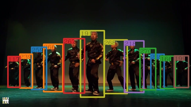
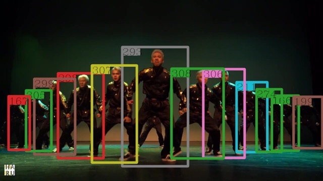
DARTH

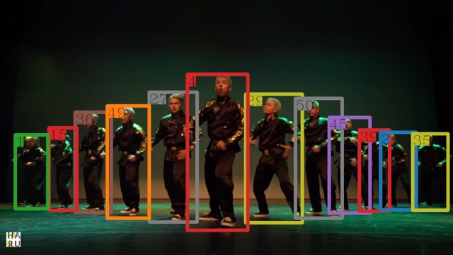
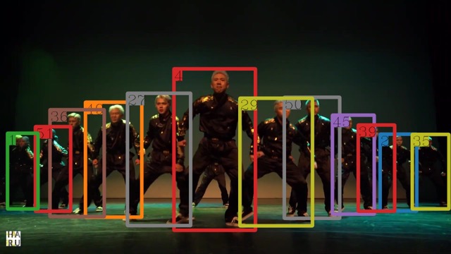
Figure 4: Tracking results on the sequence 0034 of the DanceTrack validation set in the adaptation setting $\text{MOT17}\rightarrow\text{DanceTrack}$. We analyze 2 frames spaced by $k\mkern 1.5mu{=}\mkern 1.5mu\text{0.5}$ seconds and visualize the No Adap. baseline (top row) and DARTH (bottom row). On each row, boxes of the same color correspond to the same tracking ID.

$\text{MOT17}\leftrightarrow\text{DanceTrack}$. We compare different tta adaptation methods on indoor-outdoor and contextual shifts on the MOT17 and DanceTrack datasets in Table 3. As reported in Table 1, DanceTrack poses a great challenge to the data association of a tracker trained on MOT17. We show that DARTH almost doubles the initial AssA of the non-adapted source model, and increases the MOTA and HOTA by a remarkable +12.9 and +10.1, considerably bridging the gap with an Oracle model directly trained on the target domain DanceTrack. More limited is the performance boost in the opposite direction, where our proposal improves the source model over all metrics, but the DetA gap with the Oracle model remains large. Qualitative results before and after adaptation with DARTH on $\text{MOT17}\rightarrow\text{DanceTrack}$ are shown in Figure 4. The unadapted source model correctly detects the dancers but fails at associating them, while DARTH effectively recovers instance association.

$\text{Pedestrians}\leftrightarrow\text{BDD100K}$. Data annotation is an expensive procedure, especially in video tasks such as mot. Being able to train on limited labeled data and generalize to large and diverse unlabeled datasets would save enormous annotation costs and time. Table 5 shows how, after adapting an MOT17 model to BDD100K with DARTH, the gap with the Oracle trained on BDD100K is drastically reduced, with our DARTH model far exceeding the Oracle’s MOTA. When pre-training on CrowdHuman, DARTH even ties the Oracle’s DetA, although there is still room for improving data association. In contrast, SFOD only marginally satisfies its objective of improving the DetA, while worsening all tracking-related metrics by not adapting data association.

Our method reports improvements also in the opposite direction (Table 4), where the tracker is first trained on the large scale dataset BDD100K and then asked to generalize to the smaller scale datasets MOT17 and DanceTrack. Nevertheless, the SFOD baseline also shows improvements on ${\text{BDD100K}\rightarrow\text{MOT17}}$, slightly exceeding DARTH’s DetA.

4.3 Ablation Studies

We here ablate on different design choices and components of DARTH, highlighting the importance of a holistic solution to the mot adaptation problem. Additional ablations and visual results are provided in the Appendix.

Method Components. We ablate on the impact of different method components - i.e. exponential moving average (EMA), detection consistency (DC), and patch contrastive learning (PCL) - on ${\text{SHIFT}\rightarrow\text{BDD100K}}$ in Table 6. We find that applying pcl alone is detrimental, since the newly learned features become incompatible with the unadapted detection head. Applying dc alone produces instead improvements over all metrics, and in particular over the MOTA, hinting at the enhanced consistency of detection results in adjacent frames. Enabling the momentum updates to the teacher (EMA + DC) causes a remarkable boost, meaning that the adapted global representations fostered by DC and gradually injected into the teacher generate better targets for our DC formulation. Finally, the pcl further boosts the performance of ema + dc, proving how all tracking components are interconnected and a holistic solution is required to achieve the best adaptation performance.

Data Augmentation.

EMA	DC	PCL	DetA	MOTA	HOTA	IDF1	AssA
[HTML]EFEFEF-	-	-	12.0	-66.4	17.3	18.5	28.9
[HTML]FEF4E7-	[HTML]FEF4E7-	[HTML]FEF4E7✓	9.4	-40.5	14.3	14.5	27.6
[HTML]FEF4E7-	[HTML]FEF4E7✓	[HTML]FEF4E7-	12.6	-37.6	18.0	19.5	29.5
[HTML]FEF4E7✓	[HTML]FEF4E7✓	[HTML]FEF4E7-	14.5	6.1	19.7	22.0	31.0
[HTML]FEF4E7✓	[HTML]FEF4E7✓	[HTML]FEF4E7✓	15.2	8.3	20.6	23.7	33.1

Table 6: Ablation study on the impact of different method components on DARTH (Average). We analyze the effect of different method components on DARTH (ours) on ${\text{SHIFT}\rightarrow\text{BDD100K}}$. We report with a ✓whether exponential moving average (EMA), detection consistency (DC) and Patch Contrastive Learning (PCL) are applied. For each metric we report its average across all object categories. No Adap. is in gray.

Teacher	Student	Contrastive	DetA	MOTA	HOTA	IDF1	AssA
[HTML]EFEFEF-	-	-	12.0	-66.4	17.3	18.5	28.9
[HTML]FEF4E7-	[HTML]FEF4E7-	[HTML]FEF4E7-	12.0	-39.9	14.2	13.1	21.7
[HTML]FEF4E7g	[HTML]FEF4E7-	[HTML]FEF4E7g	13.7	-7.4	19.3	21.4	32.3
[HTML]FEF4E7g	[HTML]FEF4E7-	[HTML]FEF4E7g + p	13.5	-5.8	18.9	20.8	31.3
[HTML]FEF4E7g + p	[HTML]FEF4E7-	[HTML]FEF4E7g + p	13.2	-6.8	18.5	20.4	30.5
[HTML]FEF4E7g	[HTML]FEF4E7p	[HTML]FEF4E7g	15.1	7.4	20.2	23.0	32.2
[HTML]FEF4E7g	[HTML]FEF4E7p	[HTML]FEF4E7g + p	15.2	8.3	20.6	23.7	33.1

Table 7: Ablation study on different data augmentation settings for DARTH (Average). We analyze the effect of different data augmentation settings on DARTH on ${\text{SHIFT}\rightarrow\text{BDD100K}}$. We report the augmentations applied on the Teacher, Student and Contrastive view, chosen from geometric (g) and photometric (p) augmentations as detailed in Section 3.2. For each metric we report its average across all object categories. No Adap. is in gray.

We ablate on the effect of different data augmentation strategies to generate the teacher, student, and contrastive views. The results, reported in Table 7, show how applying independent geometric augmentations to the teacher/student and contrastive views already boosts the overall performance. However, a significant additional improvement is caused by adding a subsequent photometric augmentation when generating the student view from the teacher view, making the detection consistency a consistency to photometric augmentations problem. This results in a further +15.1 in MOTA, proving that a by-product of our photometric detection consistency formulation is stabilization of detections through time.

Stronger Source Model. We investigate the impact of a stronger source model by pre-training Faster R-CNN on CrowdHuman (CH) [57] before training QDTrack on MOT17. Although this results in a marginal improvement on the source domain MOT17 (Table 1), it significantly boosts the robustness of the source model by up to +9.4 DetA and +6.8 AssA when tested on DanceTrack or BDD100K compared to the model only trained on MOT17. The experiments on ${\text{MOT17 (+CH)}\rightarrow\text{DanceTrack}}$ (Table 3) and on ${\text{MOT17 (+CH)}\rightarrow\text{BDD100K}}$ (Table 5) demonstrate that, even when starting from a more robust initialization, DARTH still significantly improves No Adap. by up to +4.0 DetA, +4.3 HOTA, and +3.8 AssA.

5 Conclusion

Playing a pivotal role in perception systems for safety-critical applications such as autonomous driving, mot algorithms must cope with unseen conditions to avoid life-critical failures. In this paper, we introduce DARTH, the first domain adaptation method for multiple object tracking. DARTH provides a holistic framework for tta of appearance-based mot by jointly adapting all the tracking components and their intrinsic relationship to the target domain. Our detection consistency formulation adapts the object detection stage by learning global representations on the target domain while enforcing detection consistency to view changes. Our patch contrastive loss adapts the appearance representations to the target domain, fostering discriminative local instance representations suitable for downstream association. Experimental results validate the remarkable effectiveness of DARTH, fostering an all-round improvement to mot in both the object detection and instance association stages on a variety of domain shifts.

Appendix

We here present additional details on the experimental setting (Section A), investigate the effect of domain shift on motion-based tracking (Section B), report additional results and ablations (Section C), and provide extensive qualitative results on the effectiveness of DARTH (Section D).

An additional video teasing DARTH and its tta efficacy is attached to this submission.

A Experimental Setting

All our models are trained with a total batch size of 16 across 8 GPU NVIDIA RTX 2080Ti.

A.1 Source Model Training

We train QDTrack on the source dataset using the SGD optimizer and a total batch size of 16, starting from an initial lr of 0.01 which is decayed on a dataset-dependent schedule.

MOT17/DanceTrack. We train QDTrack on MOT17 and DanceTrack for 4 epochs, decaying the learning rate by a factor of 10 after 3 epochs. We follow the training hyperparameters provided in MMTracking [11]. Images are first rescaled to a random width within [0.8$\cdot$1088, 1.2$\cdot$1088] maintaining the original aspect ratio, and horizontally flipped with a probability of 0.5. We then apply an ordered sequence of the following photometric augmentations, each with probability 0.5, following the MMTracking [11] implementation of the SeqPhotoMetricDistortion class with the default parameters: random brightness, random contrast (mode 0), convert color from BGR to HSV, random saturation, random hue, convert color from HSV to BGR, random contrast (mode 1), randomly swap channels. Images are then cropped to a maximum width of 1088. Finally, we normalize images using the reference ImageNet statistics, i.e. channel-wise mean (123.675, 116.28, 103.53) and standard deviation (58.395, 57.12, 57.375). When generating a training batch, all images are padded with zeros on the bottom-right corner to the size of the largest image in the batch.

SHIFT. When training on SHIFT, we train for 5 epochs and decay the learning rate by a factor of 10 after 4 epochs. Images are rescaled to the closest size in the set {(1296, 640), (1296, 672), (1296, 704), (1296, 736), (1296, 768), (1296, 800), (1296, 720)} and horizontally flipped with a probability of 0.5. Finally, images are normalized using the reference ImageNet statistics, i.e. channel-wise mean (123.675, 116.28, 103.53) and standard deviation (58.395, 57.12, 57.375). When generating a training batch, all images are padded with zeros on the bottom-right corner to the size of the largest image in the batch.

BDD100K. When training on BDD100K, we train for 12 epochs and decay the learning rate by a factor of 10 after 8 and 11 epochs. Images are rescaled to the closest size in the set {(1296, 640), (1296, 672), (1296, 704), (1296, 736), (1296, 768), (1296, 800), (1296, 720)} and horizontally flipped with a probability of 0.5. Finally, images are normalized using the reference ImageNet statistics, i.e. channel-wise mean (123.675, 116.28, 103.53) and standard deviation (58.395, 57.12, 57.375). When generating a training batch, all images are padded with zeros on the bottom-right corner to the size of the largest image in the batch.

A.2 Adapting to the Target Domain

We train DARTH on the target domain using the SGD optimizer and a total batch size of 16, starting from an initial lr of 0.001 which is decayed on a dataset-dependent schedule. In particular, we train DARTH on MOT17 and DanceTrack for 4 epochs, decaying the learning rate by a factor of 10 after 3 epochs. When training on BDD100K, we train for 10 epochs and decay the learning rate by a factor of 10 after 8 epochs. For each dataset, we adopt the same image normalization parameters as the one used for the original source model.

During the adaptation phase, the teacher model is updated as an ema of the student weights with a momentum $\tau\mkern 1.5mu{=}\mkern 1.5mu\mkern 1.5mu0.998$.

Data Augmentation. We here provide details and hyperparameters for the data augmentation transformations employed in the generation of our target, student and constrastive view. To generate the teacher view, we apply a sequence of geometric transformations. Images are first rescaled to a random width within [0.8$\cdot$1088, 1.2$\cdot$1088] maintaining the original aspect ratio, and then cropped to a maximum width of 1088 pixels. Random horizontal flipping is also applied with a probability of 0.5. When generating a training batch, all images are padded with zeros on the bottom-right corner to the size of the largest image in the batch. Given the teacher view, we generate the student view by consecutive application of photometric augmentations. Generating the student view from the teacher view is necessary to ensure geometric consistency between teacher and student views, as required by our detection consistency losses (Section 3.4). In particular, we apply an ordered sequence of the following augmentations, each with probability 0.5, following the MMTracking [11] implementation of the SeqPhotoMetricDistortion class with the default parameters: random brightness, random contrast (mode 0), convert color from BGR to HSV, random saturation, random hue, convert color from HSV to BGR, random contrast (mode 1), randomly swap channels. The contrastive view is generated using the same strategy as the student view but from independently sampled parameters of the geometric and photometric augmentations.

Table 8: Appearance-based mot (QDTrack [47])

Source	Target	DetA	MOTA	HOTA	IDF1	AssA
	[HTML]E0FCE0SHIFT	[HTML]E0FCE046.9	[HTML]E0FCE048.4	[HTML]E0FCE055.2	[HTML]E0FCE060.6	[HTML]E0FCE065.8
SHIFT	BDD100K	12.0	-66.4	17.3	18.5	28.9
	[HTML]E0FCE0MOT17	[HTML]E0FCE057.2	[HTML]E0FCE068.2	[HTML]E0FCE057.1	[HTML]E0FCE068.5	[HTML]E0FCE057.4
	DanceTrack	52.4	57.2	21.5	19.5	9.0
MOT17	BDD100K	23.2	10.5	27.2	33.3	32.4
	[HTML]E0FCE0MOT17	[HTML]E0FCE059.8	[HTML]E0FCE071.7	[HTML]E0FCE059.7	[HTML]E0FCE071.6	[HTML]E0FCE058.7
	DanceTrack	61.8	74.0	31.1	29.6	15.8
MOT17 (+CH)	BDD100K	32.4	28.3	33.7	41.7	35.4
	[HTML]E0FCE0DanceTrack	[HTML]E0FCE068.5	[HTML]E0FCE079.2	[HTML]E0FCE043.5	[HTML]E0FCE042.3	[HTML]E0FCE028.0
	MOT17	24.7	23.3	32.6	35.4	43.5
DanceTrack	BDD100K	9.3	-16.0	14.1	12.3	21.8
	[HTML]E0FCE0BDD100K	[HTML]E0FCE036.5	[HTML]E0FCE014.2	[HTML]E0FCE039.6	[HTML]E0FCE048.2	[HTML]E0FCE043.3
	MOT17	28.6	31.4	36.0	43.5	45.8
BDD100K	DanceTrack	41.9	41.6	18.0	17.0	7.9

Table 9: Motion-based mot (ByteTrack^† [77])

Source	Target	DetA	MOTA	HOTA	IDF1	AssA
	[HTML]E0FCE0SHIFT	[HTML]E0FCE046.7	[HTML]E0FCE046.6	[HTML]E0FCE055.1	[HTML]E0FCE060.6	[HTML]E0FCE065.7
SHIFT	BDD100K	11.8	-70.5	15.2	14.8	23.4
	[HTML]E0FCE0MOT17	[HTML]E0FCE056.7	[HTML]E0FCE065.8	[HTML]E0FCE057.5	[HTML]E0FCE068.9	[HTML]E0FCE058.9
	DanceTrack	52.2	62.2	31.6	35.5	19.4
MOT17	BDD100K	22.6	-12.0	21.3	22.4	20.5
	[HTML]E0FCE0MOT17	[HTML]E0FCE060.0	[HTML]E0FCE070.3	[HTML]E0FCE058.8	[HTML]E0FCE071.4	[HTML]E0FCE058.1
	DanceTrack	61.1	75.2	36.1	38.9	21.5
MOT17 (+ CH)	BDD100K	32.9	8.2	27.9	30.4	24.0
	[HTML]E0FCE0DanceTrack	[HTML]E0FCE065.9	[HTML]E0FCE077.8	[HTML]E0FCE040.4	[HTML]E0FCE041.5	[HTML]E0FCE025.0
	MOT17	25.3	21.6	34.4	38.2	47.3
DanceTrack	BDD100K	7.6	-19.2	13.1	10.0	22.9
	[HTML]E0FCE0BDD100K	[HTML]E0FCE035.8	[HTML]E0FCE09.4	[HTML]E0FCE029.1	[HTML]E0FCE031.9	[HTML]E0FCE024.0
	MOT17	31.0	29.5	36.3	43.8	43.2
BDD100K	DanceTrack	43.7	44.6	25.2	27.1	14.7

Table 10: Domain shift in mot. We assess the impact of domain shift on appearance-based (QDTrack [47], left), and motion-based (ByteTrack [77], right) mot. $\dagger$ indicates that we use the motion-only version of ByteTrack. We compare both trackers using a Faster R-CNN [50] object detector with a ResNet-50 [26] backbone and fpn [36]. In green the performance on the source domain. The ${\text{SHIFT}\rightarrow\text{BDD100K}}$ metrics are averaged across all object categories; only the pedestrian category is considered for other experiments. CH: CrowdHuman. The in-domain performance is aligned for both trackers, although QDTrack excels on the complex BDD100K [72]. Domain shift affects equally the DetA of both trackers, while threatening more the AssA of appearance-based mot.

B Domain Shift in Motion-based MOT

We here study the effect of domain shift on motion-based mot, and justify the importance of solving domain adaptation for appearance-based tracking. Motion- [3, 4, 20, 6, 77], appearance- [33, 68, 1, 47], and query-based [40, 61, 73] trackers are commonly used to associate instances detected by an object detector. Appearance-based tracking has proven the most versatile formulation, showing SOTA performance on a variety of benchmarks [21] and complementing motion cues for superior tracking performance [77]. On the other hand, motion-based tracking achieves competitive performance on datasets with high frame rates and low relative speed of tracked objects, while failing on complex datasets (e.g. BDD100K [21]) or on any domain at lower frame rates ([21], Fig. 3).

B.1 Domain Shift in Appearance- and Motion-based Multiple Object Tracking

Intuitively, all categories (appearance-, motion-, and query-based) suffer from domain shift in their detection stage. Moreover, query-based tracking can be seen as an instance of appearance-based, where the queries serve as appearance representation. We study in Table 10 the effect of domain shift on appearance- and motion-based tracking.

We choose QDTrack [47] as representative of appearance-only tracking as it provides the most effective formulation [21] to learn appearance representations for downstream instance association. We choose ByteTrack [77] as representative of motion-only tracking, as its motion-based matching scheme reports state-of-the-art performance. Although ByteTrack can also be extended to use appearance-cues, for the scope of this comparison we only use its motion component, as we intend to disentangle the effect of domain shift on appearance-only and motion-only mot. In our experiments, we compare both tracking algorithms using a Faster R-CNN [50] object detector with a ResNet-50 [26] backbone and fpn [36]. We choose the same detector for a fair comparison.

In-domain Comparison. Table 10 shows that both QDTrack (left) and the motion-only version of ByteTrack (right) obtain comparable in-domain performance (green rows) on almost all datasets. However, motion-based tracking suffers from the complexity and low frame rate of BDD100K, making a case for the use of appearance-based trackers in complex scenarios.

Domain Shift Comparison. Despite the superior versatility of appearance-based trackers, we find (Table 10, left) that appearance-based tracking suffers from domain shift in both its detection and instance association stage, due to the learning-based nature of the object detector and the appearance embedding head. On the other hand, motion-based tracking is affected less by domain shift in its data association stage. In particular, we observe that (1) the in-domain performance is aligned for both trackers, except on BDD100K, highlighting that appearance-based trackers work best in complex scenarios; (2) the drop in DetA under domain shift is comparable for both types of trackers; (3) except when shifting to BDD100K, the motion-based ByteTrack generally retains higher AssA than the appearance-based QDTrack under domain shift. This highlights the importance of domain adaptation for appearance-based mot. Although appearance-based mot achieves SOTA performance in-domain, it suffers significantly more from domain shift, making a solution to the adaptation problem desirable.

Method	Source	Target	DetA	MOTA	HOTA	IDF1	AssA
QDTrack [47]	SHIFT	BDD100K	12.0	-66.4	17.3	18.5	28.9
ByteTrack [77]			11.8	-70.5	15.2	14.8	23.4
DARTH			15.2	8.3	20.6	23.7	33.1
QDTrack [47]	MOT17	DT	52.4	57.2	21.5	19.5	9.0
ByteTrack [77]			52.2	62.2	31.6	35.5	19.4
DARTH			57.2	70.1	31.6	32.8	17.7
QDTrack [47]	MOT17 (+ CH)	DT	61.8	74.0	31.1	29.6	15.8
ByteTrack [77]			61.1	75.2	36.1	38.9	21.5
DARTH			64.7	78.9	35.4	35.3	19.6
QDTrack [47]	DT	MOT17	24.7	23.3	32.6	35.4	43.5
ByteTrack [77]			25.3	21.6	34.4	38.2	47.3
DARTH			26.4	25.5	34.3	37.9	45.2
QDTrack [47]	BDD100K	MOT17	28.6	31.4	36.0	43.5	45.8
ByteTrack [77]			31.0	29.5	36.3	43.8	43.2
DARTH			29.4	32.6	36.6	44.4	45.9
QDTrack [47]	BDD100K	DT	41.9	41.6	18.0	17.0	7.9
ByteTrack [77]			43.7	44.6	25.2	27.1	14.7
DARTH			45.1	50.2	21.5	21.4	10.4
QDTrack [47]	DT	BDD100K	9.3	-16.0	14.1	12.3	21.8
ByteTrack [77]			7.6	-19.2	13.1	10.0	22.9
DARTH			12.8	-1.5	17.8	17.4	25.1
QDTrack [47]	MOT17	BDD100K	23.2	10.5	27.2	33.3	32.4
ByteTrack [77]			22.6	-12.0	21.3	22.4	20.5
DARTH			31.6	21.4	32.4	40.4	33.6
QDTrack [47]	MOT17 (+ CH)	BDD100K	32.4	28.3	33.7	41.7	35.4
ByteTrack [77]			32.9	8.2	27.9	30.4	24.0
DARTH			36.3	23.4	36.3	44.4	36.8

Table 11: Comparison of appearance- and motion-based mot under domain shift. We compare the performance under domain shift of appearance-based (QDTrack), motion-based (ByteTrack), and domain adaptive appearance-based (DARTH, ours) mot. We use the motion-only version of ByteTrack. Both trackers use a Faster R-CNN [50] object detector with a ResNet-50 [26] backbone and fpn [36]. The ${\text{SHIFT}\rightarrow\text{BDD100K}}$ metrics are averaged across all categories; only the pedestrian category is considered in other experiments. DT: DanceTrack; CH: CrowdHuman.

Recovering Appearance-based MOT. We now investigate whether our proposed method (DARTH) can recover the performance of appearance-based trackers under domain shift, closing the gap with motion-based trackers under domain shift or even outperforming them. Table 11 compares the performance of QDTrack (appearance-based), ByteTrack (motion-based), and DARTH (domain-adaptive QDTrack) on the shifted domain. DARTH consistently outperforms DetA and MOTA of both QDTrack and ByteTrack. Moreover, it considerably recovers the AssA of QDTrack, outperforming also ByteTrack on shifts to BDD100K and reporting competitive performance to it on pedestrian datasets. Such results highlight the effectiveness of our proposed method DARTH, making a case for the use of our domain adaptive appearance-based tracker under domain shift instead of motion-based ones.

C Additional Results

We extend Section 4 with additional results.

C.1 Extension of the Ablation Study

${\text{SHIFT}\rightarrow\text{BDD100K}}$ (Overall). We here complement the main manuscript results by reporting the Overall performance on the ${\text{SHIFT}\rightarrow\text{BDD100K}}$ experiments. By Overall we mean that for each metric we report the results over all the identities available in the dataset and across all categories, as opposed to the Average results reported in the main paper which are averaged over the category-specific metrics. We make the choice of reporting the Average performance in the main paper because we believe that it is significant towards the evaluation of tta in a class-imbalanced setting. Nevertheless, we here report the absolute performance over the whole dataset for completeness. Table 12 confirms the superiority of DARTH over the considered baselines; Table 13 confirms that our chosen augmentation policy outperforms all possible alternatives; Table 14 confirms the effectiveness and complementarity of each of our method components.

${\text{MOT17}\rightarrow\text{DanceTrack}}$. We extend the ablations on method components (Table 15) and data augmentation settings (Table 16) to the ${\text{MOT17}\rightarrow\text{DanceTrack}}$ setting, further confirming the findings reported in Section 4.3.

C.2 Ablation on Confidence Threshold

We ablate on the sensitivity to the confidence threshold value in SFOD and DARTH on ${\text{SHIFT}\rightarrow\text{BDD100K}}$ and ${\text{MOT17}\rightarrow\text{DanceTrack}}$. Notice that SFOD and DARTH use the threshold differently. SFOD uses it to only retain high-confidence detections as pseudo-labels for self-training the detector. DARTH leverages a confidence threshold over the teacher detections to identify the object regions used in our patch contrastive learning formulation, as described in Section 3.3 and illustrated in Figure 3.

SFOD. We report the average (Table 17) and overall (Table 18) performance of SFOD under different thresholds on the ${\text{SHIFT}\rightarrow\text{BDD100K}}$ setting, and find that SFOD is highly sensitive to the confidence threshold choice. In particular, the average performance always worsens except when the threshold is set at 0.7, while the overall performance improves also with a threshold of 0.5. This indicates that domain shift impacts differently each category and a unique threshold for all categories is suboptimal.

DARTH. First, we report the average (Table 17) and overall (Table 18) performance of DARTH under different thresholds on the ${\text{SHIFT}\rightarrow\text{BDD100K}}$ setting, and find that DARTH is highly sensitive to the confidence threshold choice. Table 19 Table 20 The same trend is confirmed on the ${\text{MOT17}\rightarrow\text{DanceTrack}}$ setting (Table 21).

Method	Source	Target	DetA	MOTA	HOTA	IDF1	AssA
No Adap.	SHIFT	BDD100K	27.2	20.4	35.1	39.5	46.4
Tent [65]			0.3	0.2	1.9	0.5	14.8
SFOD [35]			27.7	22.7	35.7	40.0	47.1
Ours			36.5	33.3	43.1	50.9	51.8
[HTML]EFEFEFOracle	BDD100K	BDD100K	55.9	58.5	59.7	69.2	64.6

Table 12: State of the art on ${\textbf{SHIFT}\rightarrow\textbf{BDD100K}}$ (Overall). We benchmark DARTH (ours) against baseline test-time adaptation methods for adapting a mot model from the synthetic driving dataset SHIFT to the real-world BDD100K. For each metric we report the overall result across all categories.

Teacher	Student	Contrastive	DetA	MOTA	HOTA	IDF1	AssA
[HTML]EFEFEF-	-	-	27.2	20.4	35.1	39.5	46.4
[HTML]FEF4E7-	[HTML]FEF4E7-	[HTML]FEF4E7-	26.8	12.5	27.7	25.8	29.7
[HTML]FEF4E7g	[HTML]FEF4E7-	[HTML]FEF4E7g	31.4	28.5	39.2	45.2	50.0
[HTML]FEF4E7g	[HTML]FEF4E7-	[HTML]FEF4E7g + p	31.2	28.8	39.0	45.1	49.6
[HTML]FEF4E7g + p	[HTML]FEF4E7-	[HTML]FEF4E7g + p	30.3	27.9	38.5	44.3	49.8
[HTML]FEF4E7g	[HTML]FEF4E7p	[HTML]FEF4E7g	37.0	32.8	43.2	50.8	51.6
[HTML]FEF4E7g	[HTML]FEF4E7p	[HTML]FEF4E7g + p	36.5	33.3	43.1	50.9	51.8

Table 13: Ablation study on different data augmentation settings for DARTH (Overall). We analyze the effect of different data augmentation settings on DARTH on ${\text{SHIFT}\rightarrow\text{BDD100K}}$. We report the augmentations applied on the Teacher, Student and Contrastive view, chosen from geometric (g) and photometric (p) augmentations as detailed in Section 3.2. For each metric we report the overall result across all categories. No Adap. is in gray.

EMA	DC	PCL	DetA	MOTA	HOTA	IDF1	AssA
[HTML]EFEFEF-	-	-	27.2	20.4	35.1	39.5	46.4
[HTML]FEF4E7-	[HTML]FEF4E7-	[HTML]FEF4E7✓	23.8	8.3	29.6	34.7	37.6
[HTML]FEF4E7-	[HTML]FEF4E7✓	[HTML]FEF4E7-	28.0	23.0	36.1	40.6	47.6
[HTML]FEF4E7✓	[HTML]FEF4E7✓	[HTML]FEF4E7-	33.8	32.0	40.8	46.9	50.3
[HTML]FEF4E7✓	[HTML]FEF4E7✓	[HTML]FEF4E7✓	36.5	33.3	43.1	50.9	51.8

Table 14: Ablation study on the impact of different method components on DARTH (Overall). We analyze the effect of different method components on DARTH (ours) on ${\text{SHIFT}\rightarrow\text{BDD100K}}$. We report with a ✓whether exponential moving average (EMA), detection consistency (DC) and Patch Contrastive Learning (PCL) are applied. For each metric we report the overall result across all categories. No Adap. is in gray.

EMA	DC	PCL	DetA	MOTA	HOTA	IDF1	AssA
[HTML]EFEFEF-	-	-	52.4	57.2	21.5	19.5	9.0
[HTML]FEF4E7-	[HTML]FEF4E7-	[HTML]FEF4E7✓	51.2	54.1	28.3	28.6	16.0
[HTML]FEF4E7-	[HTML]FEF4E7✓	[HTML]FEF4E7-	52.7	58.0	21.8	19.7	9.2
[HTML]FEF4E7✓	[HTML]FEF4E7✓	[HTML]FEF4E7-	55.3	62.0	23.3	21.4	10.0
[HTML]FEF4E7✓	[HTML]FEF4E7✓	[HTML]FEF4E7✓	57.2	70.1	31.6	32.8	17.7

Table 15: Ablation study on the impact of different method components on DARTH (${\textbf{MOT17}\rightarrow\textbf{DanceTrack}}$). We analyze the effect of different method components on DARTH (ours) on ${\text{MOT17}\rightarrow\text{DanceTrack}}$. We report with a ✓whether exponential moving average (EMA), detection consistency (DC) and Patch Contrastive Learning (PCL) are applied. No Adap. is in gray.

Teacher	[HTML]FFFFFFStudent	[HTML]FFFFFFContrastive	DetA	MOTA	HOTA	IDF1	AssA
[HTML]EFEFEF-	-	-	52.4	57.2	21.5	19.5	9.0
[HTML]FEF4E7-	-	-	52.5	29.9	12.4	9.2	3.1
[HTML]FEF4E7g	-	g	54.7	66.9	30.8	32.2	17.6
[HTML]FEF4E7g	-	g + p	54.7	66.9	31.5	33.6	18.3
[HTML]FEF4E7g + p	-	g + p	54.6	66.7	30.7	32.2	17.5
[HTML]FEF4E7g	p	g + p	57.2	70.1	31.6	32.8	17.7

Table 16: Ablation study on different data augmentation settings for DARTH (${\textbf{MOT17}\rightarrow\textbf{DanceTrack}}$). We analyze the effect of different data augmentation settings on DARTH on ${\text{MOT17}\rightarrow\text{DanceTrack}}$. We report the augmentations applied on the Teacher, Student and Contrastive view, chosen from geometric (g) and photometric (p) augmentations as detailed in Section 3.2. No Adap. is in gray.

Conf. Thr.	DetA	MOTA	HOTA	IDF1	AssA
[HTML]EFEFEF-	12.0	-66.4	17.3	18.5	28.9
[HTML]FEF4E70.0	7.9	-841.7	12.8	10.8	28.5
[HTML]FEF4E70.3	11.2	-258.2	16.2	16.2	29.2
[HTML]FEF4E70.5	12.0	-135.1	17.2	17.8	29.6
[HTML]FEF4E70.7	12.4	-57.3	17.7	19.0	29.1
[HTML]FEF4E70.9	11.9	-5.4	17.5	19.3	28.7

Table 17: Ablation study on confidence thresholds for SFOD [35] (Average). We analyze the sensitivity of SFOD to different confidence thresholds for the detection pseudo labels filtering on ${\text{SHIFT}\rightarrow\text{BDD100K}}$. For each metric we report its average across all object categories. No Adap. is in gray.

Conf. Thr.	DetA	MOTA	HOTA	IDF1	AssA
[HTML]EFEFEF-	27.2	20.4	35.1	39.5	46.4
[HTML]FEF4E70.0	19.4	-81.4	27.8	26.3	41.9
[HTML]FEF4E70.3	27.0	1.9	34.4	37.5	45.3
[HTML]FEF4E70.5	27.8	15.2	35.6	39.5	46.7
[HTML]FEF4E70.7	27.7	22.7	35.7	40.0	47.1
[HTML]FEF4E70.9	25.0	25.2	34.4	37.7	48.1

Table 18: Ablation study on confidence thresholds for SFOD [35] (Overall). We analyze the sensitivity of SFOD to different confidence thresholds for the detection pseudo labels filtering on ${\text{SHIFT}\rightarrow\text{BDD100K}}$. For each metric we report the overall result across all categories. No Adap. is in gray.

Conf. Thr.	DetA	MOTA	HOTA	IDF1	AssA
[HTML]EFEFEF-	12.0	-66.4	17.3	18.5	28.9
[HTML]FEF4E70.0	14.6	5.2	19.8	22.2	31.4
[HTML]FEF4E70.3	14.9	7.8	20.0	22.8	31.7
[HTML]FEF4E70.5	15.2	7.6	20.3	23.0	32.2
[HTML]FEF4E70.7	15.2	8.3	20.6	23.7	33.1
[HTML]FEF4E70.9	14.7	7.5	19.6	22.3	31.4

Table 19: Ablation study on confidence thresholds for DARTH (Average). We analyze the sensitivity of DARTH (Ours) to different confidence thresholds for filtering detection in our self-matching stage on ${\text{SHIFT}\rightarrow\text{BDD100K}}$. For each metric we report its average across all object categories. No Adap. is in gray.

Conf. Thr.	DetA	MOTA	HOTA	IDF1	AssA
[HTML]EFEFEF-	27.2	20.4	35.1	39.5	46.4
[HTML]FEF4E70.0	35.2	32.5	42.2	49.4	51.7
[HTML]FEF4E70.3	36.2	33.2	43.2	50.9	52.5
[HTML]FEF4E70.5	36.6	33.3	43.0	50.8	51.7
[HTML]FEF4E70.7	36.5	33.3	43.1	50.9	51.8
[HTML]FEF4E70.9	36.4	32.7	42.8	50.2	51.2

Table 20: Ablation study on confidence thresholds for DARTH (Overall). We analyze the sensitivity of DARTH (Ours) to different confidence thresholds for filtering detection in our self-matching stage on ${\text{SHIFT}\rightarrow\text{BDD100K}}$. For each metric we report the overall result across all categories. No Adap. is in gray.

Conf. Thr.	DetA	MOTA	HOTA	IDF1	AssA
[HTML]EFEFEF-	52.4	57.2	21.5	19.5	9.0
[HTML]FEF4E70.0	56.4	68.4	30.1	30.8	16.3
[HTML]FEF4E70.3	56.6	69.5	31.6	33.0	17.9
[HTML]FEF4E70.5	56.8	69.4	31.7	32.9	17.9
[HTML]FEF4E70.7	57.2	70.1	31.6	32.8	17.7
[HTML]FEF4E70.9	57.0	70.1	32.0	33.5	18.2

Table 21: Ablation study on confidence thresholds for DARTH (${\textbf{MOT17}\rightarrow\textbf{DanceTrack}}$). We analyze the sensitivity of DARTH (Ours) to different confidence thresholds for filtering detections in our self-matching stage on ${\text{MOT17}\rightarrow\text{DanceTrack}}$. No Adap. is in gray.

Momentum	DetA	MOTA	HOTA	IDF1	AssA
[HTML]EFEFEF-	12.0	-66.4	17.3	18.5	28.9
[HTML]FEF4E71.0	12.8	-32.1	17.9	19.4	28.5
[HTML]FEF4E70.998	15.2	8.3	20.6	23.7	33.1
[HTML]FEF4E70.98	5.9	-21.6	9.1	9.3	17.5

Table 22: Ablation study on EMA momentum for DARTH (Average). We analyze the sensitivity of DARTH (Ours) to different values of the ema momentum used to update the teacher on ${\text{SHIFT}\rightarrow\text{BDD100K}}$. For each metric we report its average across all object categories. No Adap. is in gray.

Momentum	DetA	MOTA	HOTA	IDF1	AssA
[HTML]EFEFEF-	27.2	20.4	35.1	39.5	46.4
[HTML]FEF4E71.0	28.2	23.5	36.3	41.1	47.8
[HTML]FEF4E70.998	36.5	33.3	43.1	50.9	51.8
[HTML]FEF4E70.98	17.3	-102.9	26.8	26.0	43.4

Table 23: Ablation study on EMA momentum for DARTH (Overall). We analyze the sensitivity of DARTH (Ours) to different values of the ema momentum used to update the teacher on ${\text{SHIFT}\rightarrow\text{BDD100K}}$. For each metric we report the overall result across all categories. No Adap. is in gray.

C.3 Ablation on EMA Momentum.

We ablate on the effect on DARTH of different momentum choices for the EMA update of the teacher model, as described in Section 3.2. We report the average (Table 17) and overall (Table 18) performance of DARTH under different momentum values on the ${\text{SHIFT}\rightarrow\text{BDD100K}}$ setting. We find that, while DARTH improves the baseline performance also with a frozen teacher (momentum 1.0), a suitable choice of the momentum (momentum 0.998) allows to incorporate in the teacher model the improved student weights and provide better targets for the detection consistency loss, remarkably boosting the overall performance. However, if the update to the teacher is too fast (momentum 0.98), we hypothesize that the encoder and its adapted representations may update the teacher too quickly and deviate from the expected distribution to the detection head.

D Qualitative Results

We provide extensive qualitative results on the effectiveness of DARTH on the ${\text{MOT17}\rightarrow\text{DanceTrack}}$ and ${\text{SHIFT}\rightarrow\text{BDD100K}}$ settings. In particular, we compare the No Adap. baseline and DARTH by visualizing representative examples of their tracking results, their false negative detections, and their ID switches. For each method, we show 5 adjacent frames.

D.1 MOT17 $\rightarrow$ DanceTrack

We compare the No Adap. baseline and DARTH on the MOT17 $\rightarrow$ DanceTrack setting, providing qualitative results on how DARTH can recover false negative detections and ID switches.

Recovering False Negative Detections. We analyze two crowded scenes and visualize for each the tracking results, the false positive detections, and the ID switches: (Figures 5, 6 and 7), and (Figures 8, 9 and 10). It appears evident in Figure 6 and Figure 9 how DARTH drastically recovers false negative detections (orange) by identifying correct matches (green). At the same time, even though DARTH is able to detect and track more objects, also the number of ID switches reduces (Figures 7 and 10), hinting at the improved association performance.

Recovering ID Switches. We further consider a variety of scenes with a reduced amount of objects where the No Adap. baseline already does not suffer from false negatives, and show how DARTH drastically reduces ID switches. This can be seen on the following pairs of tracking results and visualizations of ID switches: (Figures 11 and 12), (Figures 13 and 14), (Figures 15 and 16), and (Figures 17 and 18). In most of these cases, DARTH does not suffer ID switches in the considered frames, as opposed to the No Adap. baseline. Nevertheless, an example of ID switch (blue) with DARTH can be identified in Figure 18 at $t\mkern 1.5mu{=}\mkern 1.5mu\hat{t}+k$, where an ID switches when two dancers switch position and overlap with each other.

D.2 SHIFT $\rightarrow$ BDD100K

We compare the No Adap. baseline and DARTH on the SHIFT $\rightarrow$ BDD100K setting, providing qualitative results on how DARTH can recover false negative detections and ID switches.

Recovering False Negative Detections. We show examples of tracking results and the respective visualization of false negative detections in (Figures 19 and 20), (Figures 21 and 22), (Figures 23 and 24), and (Figures 25 and 26). DARTH is able to recover a large amount of false negative detections, especially on the road side vehicles, and correctly track them through time.

Recovering ID Switches. We show examples of tracking results and the respective visualization of ID switches in (Figures 27 and 28), (Figures 29 and 30), and (Figures 31 and 32). DARTH reduces the number of ID switches, consistently detect objects through time and correctly assigns them to the same tracklet.

	$t=\hat{t}-2k$	$t=\hat{t}-k$	$t=\hat{t}$	$t=\hat{t}+k$	$t=\hat{t}+2k$
No Adap.
DARTH

Figure 5: Tracking results on the sequence 0025 of the DanceTrack validation set in the adaptation setting $\text{MOT17}\rightarrow\text{DanceTrack}$. We analyze 5 consecutive frames centered around the frame #28 at time $\hat{t}$ and spaced by $k\mkern 1.5mu{=}\mkern 1.5mu\text{0.05}$ seconds. We visualize the No Adap. baseline (top row) and DARTH (bottom row). On each row, boxes of the same color correspond to the same tracking ID.

	$t=\hat{t}-2k$	$t=\hat{t}-k$	$t=\hat{t}$	$t=\hat{t}+k$	$t=\hat{t}+2k$
No Adap.
DARTH

Figure 6: Tracking results on the sequence 0025 of the DanceTrack validation set in the adaptation setting $\text{MOT17}\rightarrow\text{DanceTrack}$. We analyze 5 consecutive frames centered around the frame #28 at time $\hat{t}$ and spaced by $k\mkern 1.5mu{=}\mkern 1.5mu\text{0.05}$ seconds. We visualize the No Adap. baseline (top row) and DARTH (bottom row). On each row, green boxes represent correctly tracked objects, and orange boxes represent false negatives. We omit false positive boxes and ID switches for ease of visualization.

	$t=\hat{t}-2k$	$t=\hat{t}-k$	$t=\hat{t}$	$t=\hat{t}+k$	$t=\hat{t}+2k$
No Adap.
DARTH

Figure 7: Tracking results on the sequence 0025 of the DanceTrack validation set in the adaptation setting $\text{MOT17}\rightarrow\text{DanceTrack}$. We analyze 5 consecutive frames centered around the frame #28 at time $\hat{t}$ and spaced by $k\mkern 1.5mu{=}\mkern 1.5mu\text{0.05}$ seconds. We visualize the No Adap. baseline (top row) and DARTH (bottom row). On each row, green boxes represent correctly tracked objects, and blue boxes represent ID switches. We omit false positive and false negative boxes for ease of visualization.

	$t=\hat{t}-2k$	$t=\hat{t}-k$	$t=\hat{t}$	$t=\hat{t}+k$	$t=\hat{t}+2k$
No Adap.
DARTH

Figure 8: Tracking results on the sequence 0026 of the DanceTrack validation set in the adaptation setting $\text{MOT17}\rightarrow\text{DanceTrack}$. We analyze 5 consecutive frames centered around the frame #54 at time $\hat{t}$ and spaced by $k\mkern 1.5mu{=}\mkern 1.5mu\text{0.05}$ seconds. We visualize the No Adap. baseline (top row) and DARTH (bottom row). On each row, boxes of the same color correspond to the same tracking ID.

	$t=\hat{t}-2k$	$t=\hat{t}-k$	$t=\hat{t}$	$t=\hat{t}+k$	$t=\hat{t}+2k$
No Adap.
DARTH

Figure 9: Tracking results on the sequence 0026 of the DanceTrack validation set in the adaptation setting $\text{MOT17}\rightarrow\text{DanceTrack}$. We analyze 5 consecutive frames centered around the frame #54 at time $\hat{t}$ and spaced by $k\mkern 1.5mu{=}\mkern 1.5mu\text{0.05}$ seconds. We visualize the No Adap. baseline (top row) and DARTH (bottom row). On each row, green boxes represent correctly tracked objects, and orange boxes represent false negatives. We omit false positive boxes and ID switches for ease of visualization.

	$t=\hat{t}-2k$	$t=\hat{t}-k$	$t=\hat{t}$	$t=\hat{t}+k$	$t=\hat{t}+2k$
No Adap.
DARTH

Figure 10: Tracking results on the sequence 0026 of the DanceTrack validation set in the adaptation setting $\text{MOT17}\rightarrow\text{DanceTrack}$. We analyze 5 consecutive frames centered around the frame #54 at time $\hat{t}$ and spaced by $k\mkern 1.5mu{=}\mkern 1.5mu\text{0.05}$ seconds. We visualize the No Adap. baseline (top row) and DARTH (bottom row). On each row, green boxes represent correctly tracked objects, and blue boxes represent ID switches. We omit false positive and false negative boxes for ease of visualization.

	$t=\hat{t}-2k$	$t=\hat{t}-k$	$t=\hat{t}$	$t=\hat{t}+k$	$t=\hat{t}+2k$
No Adap.
DARTH

Figure 11: Tracking results on the sequence 0034 of the DanceTrack validation set in the adaptation setting $\text{MOT17}\rightarrow\text{DanceTrack}$. We analyze 5 consecutive frames centered around the frame #143 at time $\hat{t}$ and spaced by $k\mkern 1.5mu{=}\mkern 1.5mu\text{0.05}$ seconds. We visualize the No Adap. baseline (top row) and DARTH (bottom row). On each row, boxes of the same color correspond to the same tracking ID.

	$t=\hat{t}-2k$	$t=\hat{t}-k$	$t=\hat{t}$	$t=\hat{t}+k$	$t=\hat{t}+2k$
No Adap.
DARTH

Figure 12: Tracking results on the sequence 0034 of the DanceTrack validation set in the adaptation setting $\text{MOT17}\rightarrow\text{DanceTrack}$. We analyze 5 consecutive frames centered around the frame #143 at time $\hat{t}$ and spaced by $k\mkern 1.5mu{=}\mkern 1.5mu\text{0.05}$ seconds. We visualize the No Adap. baseline (top row) and DARTH (bottom row). On each row, green boxes represent correctly tracked objects, and blue boxes represent ID switches. We omit false positive and false negative boxes for ease of visualization.

	$t=\hat{t}-2k$	$t=\hat{t}-k$	$t=\hat{t}$	$t=\hat{t}+k$	$t=\hat{t}+2k$
No Adap.
DARTH

Figure 13: Tracking results on the sequence 0058 of the DanceTrack validation set in the adaptation setting $\text{MOT17}\rightarrow\text{DanceTrack}$. We analyze 5 consecutive frames centered around the frame #783 at time $\hat{t}$ and spaced by $k\mkern 1.5mu{=}\mkern 1.5mu\text{0.05}$ seconds. We visualize the No Adap. baseline (top row) and DARTH (bottom row). On each row, boxes of the same color correspond to the same tracking ID.

	$t=\hat{t}-2k$	$t=\hat{t}-k$	$t=\hat{t}$	$t=\hat{t}+k$	$t=\hat{t}+2k$
No Adap.
DARTH

Figure 14: Tracking results on the sequence 0058 of the DanceTrack validation set in the adaptation setting $\text{MOT17}\rightarrow\text{DanceTrack}$. We analyze 5 consecutive frames centered around the frame #783 at time $\hat{t}$ and spaced by $k\mkern 1.5mu{=}\mkern 1.5mu\text{0.05}$ seconds. We visualize the No Adap. baseline (top row) and DARTH (bottom row). On each row, green boxes represent correctly tracked objects, and blue boxes represent ID switches. We omit false positive and false negative boxes for ease of visualization.

	$t=\hat{t}-2k$	$t=\hat{t}-k$	$t=\hat{t}$	$t=\hat{t}+k$	$t=\hat{t}+2k$
No Adap.
DARTH

Figure 15: Tracking results on the sequence 0035 of the DanceTrack validation set in the adaptation setting $\text{MOT17}\rightarrow\text{DanceTrack}$. We analyze 5 consecutive frames centered around the frame #248 at time $\hat{t}$ and spaced by $k\mkern 1.5mu{=}\mkern 1.5mu\text{0.05}$ seconds. We visualize the No Adap. baseline (top row) and DARTH (bottom row). On each row, boxes of the same color correspond to the same tracking ID.

	$t=\hat{t}-2k$	$t=\hat{t}-k$	$t=\hat{t}$	$t=\hat{t}+k$	$t=\hat{t}+2k$
No Adap.
DARTH

Figure 16: Tracking results on the sequence 0035 of the DanceTrack validation set in the adaptation setting $\text{MOT17}\rightarrow\text{DanceTrack}$. We analyze 5 consecutive frames centered around the frame #248 at time $\hat{t}$ and spaced by $k\mkern 1.5mu{=}\mkern 1.5mu\text{0.05}$ seconds. We visualize the No Adap. baseline (top row) and DARTH (bottom row). On each row, green boxes represent correctly tracked objects, and blue boxes represent ID switches. We omit false positive and false negative boxes for ease of visualization.

	$t=\hat{t}-2k$	$t=\hat{t}-k$	$t=\hat{t}$	$t=\hat{t}+k$	$t=\hat{t}+2k$
No Adap.
DARTH

Figure 17: Tracking results on the sequence 0007 of the DanceTrack validation set in the adaptation setting $\text{MOT17}\rightarrow\text{DanceTrack}$. We analyze 5 consecutive frames centered around the frame #143 at time $\hat{t}$ and spaced by $k\mkern 1.5mu{=}\mkern 1.5mu\text{0.05}$ seconds. We visualize the No Adap. baseline (top row) and DARTH (bottom row). On each row, boxes of the same color correspond to the same tracking ID.

	$t=\hat{t}-2k$	$t=\hat{t}-k$	$t=\hat{t}$	$t=\hat{t}+k$	$t=\hat{t}+2k$
No Adap.
DARTH

Figure 18: Tracking results on the sequence 0007 of the DanceTrack validation set in the adaptation setting $\text{MOT17}\rightarrow\text{DanceTrack}$. We analyze 5 consecutive frames centered around the frame #143 at time $\hat{t}$ and spaced by $k\mkern 1.5mu{=}\mkern 1.5mu\text{0.05}$ seconds. We visualize the No Adap. baseline (top row) and DARTH (bottom row). On each row, green boxes represent correctly tracked objects, and blue boxes represent ID switches. We omit false positive and false negative boxes for ease of visualization.

	$t=\hat{t}-2k$	$t=\hat{t}-k$	$t=\hat{t}$	$t=\hat{t}+k$	$t=\hat{t}+2k$
No Adap.
DARTH

Figure 19: Tracking results on the sequence b1c66a42-6f7d68ca of the BDD100K validation set in the adaptation setting ${\text{SHIFT}\rightarrow\text{BDD100K}}$. We analyze 5 consecutive frames centered around the frame #7 at time $\hat{t}$ and spaced by $k\mkern 1.5mu{=}\mkern 1.5mu\text{0.2}$ seconds. We visualize the No Adap. baseline (top row) and DARTH (bottom row). On each row, boxes of the same color correspond to the same tracking ID.

	$t=\hat{t}-2k$	$t=\hat{t}-k$	$t=\hat{t}$	$t=\hat{t}+k$	$t=\hat{t}+2k$
No Adap.
DARTH

Figure 20: Tracking results on the sequence b1c66a42-6f7d68ca of the BDD100K validation set in the adaptation setting ${\text{SHIFT}\rightarrow\text{BDD100K}}$. We analyze 5 consecutive frames centered around the frame #7 at time $\hat{t}$ and spaced by $k\mkern 1.5mu{=}\mkern 1.5mu\text{0.2}$ seconds. We visualize the No Adap. baseline (top row) and DARTH (bottom row). On each row, green boxes represent correctly tracked objects, and orange boxes represent false negatives. We omit false positive boxes and ID switches for ease of visualization.

	$t=\hat{t}-2k$	$t=\hat{t}-k$	$t=\hat{t}$	$t=\hat{t}+k$	$t=\hat{t}+2k$
No Adap.
DARTH

Figure 21: Tracking results on the sequence b1cac6a7-04e33135 of the BDD100K validation set in the adaptation setting ${\text{SHIFT}\rightarrow\text{BDD100K}}$. We analyze 5 consecutive frames centered around the frame #44 at time $\hat{t}$ and spaced by $k\mkern 1.5mu{=}\mkern 1.5mu\text{0.2}$ seconds. We visualize the No Adap. baseline (top row) and DARTH (bottom row). On each row, boxes of the same color correspond to the same tracking ID.

	$t=\hat{t}-2k$	$t=\hat{t}-k$	$t=\hat{t}$	$t=\hat{t}+k$	$t=\hat{t}+2k$
No Adap.
DARTH

Figure 22: Tracking results on the sequence b1cac6a7-04e33135 of the BDD100K validation set in the adaptation setting ${\text{SHIFT}\rightarrow\text{BDD100K}}$. We analyze 5 consecutive frames centered around the frame #44 at time $\hat{t}$ and spaced by $k\mkern 1.5mu{=}\mkern 1.5mu\text{0.2}$ seconds. We visualize the No Adap. baseline (top row) and DARTH (bottom row). On each row, green boxes represent correctly tracked objects, and orange boxes represent false negatives. We omit false positive boxes and ID switches for ease of visualization.

	$t=\hat{t}-2k$	$t=\hat{t}-k$	$t=\hat{t}$	$t=\hat{t}+k$	$t=\hat{t}+2k$
No Adap.
DARTH

Figure 23: Tracking results on the sequence b250fb0c-01a1b8d3 of the BDD100K validation set in the adaptation setting ${\text{SHIFT}\rightarrow\text{BDD100K}}$. We analyze 5 consecutive frames centered around the frame #114 at time $\hat{t}$ and spaced by $k\mkern 1.5mu{=}\mkern 1.5mu\text{0.2}$ seconds. We visualize the No Adap. baseline (top row) and DARTH (bottom row). On each row, boxes of the same color correspond to the same tracking ID.

	$t=\hat{t}-2k$	$t=\hat{t}-k$	$t=\hat{t}$	$t=\hat{t}+k$	$t=\hat{t}+2k$
No Adap.
DARTH

Figure 24: Tracking results on the sequence b250fb0c-01a1b8d3 of the BDD100K validation set in the adaptation setting ${\text{SHIFT}\rightarrow\text{BDD100K}}$. We analyze 5 consecutive frames centered around the frame #114 at time $\hat{t}$ and spaced by $k\mkern 1.5mu{=}\mkern 1.5mu\text{0.2}$ seconds. We visualize the No Adap. baseline (top row) and DARTH (bottom row). On each row, green boxes represent correctly tracked objects, and orange boxes represent false negatives. We omit false positive boxes and ID switches for ease of visualization.

	$t=\hat{t}-2k$	$t=\hat{t}-k$	$t=\hat{t}$	$t=\hat{t}+k$	$t=\hat{t}+2k$
No Adap.
DARTH

Figure 25: Tracking results on the sequence b2064e61-2beadd45 of the BDD100K validation set in the adaptation setting ${\text{SHIFT}\rightarrow\text{BDD100K}}$. We analyze 5 consecutive frames centered around the frame #100 at time $\hat{t}$ and spaced by $k\mkern 1.5mu{=}\mkern 1.5mu\text{0.2}$ seconds. We visualize the No Adap. baseline (top row) and DARTH (bottom row). On each row, boxes of the same color correspond to the same tracking ID.

	$t=\hat{t}-2k$	$t=\hat{t}-k$	$t=\hat{t}$	$t=\hat{t}+k$	$t=\hat{t}+2k$
No Adap.
DARTH

Figure 26: Tracking results on the sequence b2064e61-2beadd45 of the BDD100K validation set in the adaptation setting ${\text{SHIFT}\rightarrow\text{BDD100K}}$. We analyze 5 consecutive frames centered around the frame #100 at time $\hat{t}$ and spaced by $k\mkern 1.5mu{=}\mkern 1.5mu\text{0.2}$ seconds. We visualize the No Adap. baseline (top row) and DARTH (bottom row). On each row, green boxes represent correctly tracked objects, and orange boxes represent false negatives. We omit false positive boxes and ID switches for ease of visualization.

	$t=\hat{t}-2k$	$t=\hat{t}-k$	$t=\hat{t}$	$t=\hat{t}+k$	$t=\hat{t}+2k$
No Adap.
DARTH

Figure 27: Tracking results on the sequence b23493b1-3200de1c of the BDD100K validation set in the adaptation setting ${\text{SHIFT}\rightarrow\text{BDD100K}}$. We analyze 5 consecutive frames centered around the frame #99 at time $\hat{t}$ and spaced by $k\mkern 1.5mu{=}\mkern 1.5mu\text{0.2}$ seconds. We visualize the No Adap. baseline (top row) and DARTH (bottom row). On each row, boxes of the same color correspond to the same tracking ID.

	$t=\hat{t}-2k$	$t=\hat{t}-k$	$t=\hat{t}$	$t=\hat{t}+k$	$t=\hat{t}+2k$
No Adap.
DARTH

Figure 28: Tracking results on the sequence b23493b1-3200de1c of the BDD100K validation set in the adaptation setting ${\text{SHIFT}\rightarrow\text{BDD100K}}$. We analyze 5 consecutive frames centered around the frame #99 at time $\hat{t}$ and spaced by $k\mkern 1.5mu{=}\mkern 1.5mu\text{0.2}$ seconds. We visualize the No Adap. baseline (top row) and DARTH (bottom row). On each row, green boxes represent correctly tracked objects, and blue boxes represent ID switches. We omit false positive and false negative boxes for ease of visualization.

	$t=\hat{t}-2k$	$t=\hat{t}-k$	$t=\hat{t}$	$t=\hat{t}+k$	$t=\hat{t}+2k$
No Adap.
DARTH

Figure 29: Tracking results on the sequence b1f4491b-97465266 of the BDD100K validation set in the adaptation setting ${\text{SHIFT}\rightarrow\text{BDD100K}}$. We analyze 5 consecutive frames centered around the frame #32 at time $\hat{t}$ and spaced by $k\mkern 1.5mu{=}\mkern 1.5mu\text{0.2}$ seconds. We visualize the No Adap. baseline (top row) and DARTH (bottom row). On each row, boxes of the same color correspond to the same tracking ID.

	$t=\hat{t}-2k$	$t=\hat{t}-k$	$t=\hat{t}$	$t=\hat{t}+k$	$t=\hat{t}+2k$
No Adap.
DARTH

Figure 30: Tracking results on the sequence b1f4491b-97465266 of the BDD100K validation set in the adaptation setting ${\text{SHIFT}\rightarrow\text{BDD100K}}$. We analyze 5 consecutive frames centered around the frame #32 at time $\hat{t}$ and spaced by $k\mkern 1.5mu{=}\mkern 1.5mu\text{0.2}$ seconds. We visualize the No Adap. baseline (top row) and DARTH (bottom row). On each row, green boxes represent correctly tracked objects, and blue boxes represent ID switches. We omit false positive and false negative boxes for ease of visualization.

	$t=\hat{t}-2k$	$t=\hat{t}-k$	$t=\hat{t}$	$t=\hat{t}+k$	$t=\hat{t}+2k$
No Adap.
DARTH

Figure 31: Tracking results on the sequence b1e8ad72-c3c79240 of the BDD100K validation set in the adaptation setting ${\text{SHIFT}\rightarrow\text{BDD100K}}$. We analyze 5 consecutive frames centered around the frame #107 at time $\hat{t}$ and spaced by $k\mkern 1.5mu{=}\mkern 1.5mu\text{0.2}$ seconds. We visualize the No Adap. baseline (top row) and DARTH (bottom row). On each row, boxes of the same color correspond to the same tracking ID.

	$t=\hat{t}-2k$	$t=\hat{t}-k$	$t=\hat{t}$	$t=\hat{t}+k$	$t=\hat{t}+2k$
No Adap.
DARTH

Figure 32: Tracking results on the sequence b1e8ad72-c3c79240 of the BDD100K validation set in the adaptation setting ${\text{SHIFT}\rightarrow\text{BDD100K}}$. We analyze 5 consecutive frames centered around the frame #107 at time $\hat{t}$ and spaced by $k\mkern 1.5mu{=}\mkern 1.5mu\text{0.2}$ seconds. We visualize the No Adap. baseline (top row) and DARTH (bottom row). On each row, green boxes represent correctly tracked objects, and blue boxes represent ID switches. We omit false positive and false negative boxes for ease of visualization.

References

- [1] Philipp Bergmann, Tim Meinhardt, and Laura Leal-Taixe. Tracking without bells and whistles. In Proceedings of the IEEE/CVF International Conference on Computer Vision, pages 941–951, 2019.
- [2] Keni Bernardin and Rainer Stiefelhagen. Evaluating multiple object tracking performance: the clear mot metrics. EURASIP Journal on Image and Video Processing, 2008:1–10, 2008.
- [3] Alex Bewley, Zongyuan Ge, Lionel Ott, Fabio Ramos, and Ben Upcroft. Simple online and realtime tracking. In 2016 IEEE international conference on image processing (ICIP), pages 3464–3468. IEEE, 2016.
- [4] Erik Bochinski, Volker Eiselein, and Thomas Sikora. High-speed tracking-by-detection without using image information. In 2017 14th IEEE international conference on advanced video and signal based surveillance (AVSS), pages 1–6. IEEE, 2017.
- [5] Qi Cai, Yingwei Pan, Chong-Wah Ngo, Xinmei Tian, Lingyu Duan, and Ting Yao. Exploring object relation in mean teacher for cross-domain detection. In Proceedings of the IEEE/CVF Conference on Computer Vision and Pattern Recognition, pages 11457–11466, 2019.
- [6] Jinkun Cao, Xinshuo Weng, Rawal Khirodkar, Jiangmiao Pang, and Kris Kitani. Observation-centric sort: Rethinking sort for robust multi-object tracking. arXiv preprint arXiv:2203.14360, 2022.
- [7] Chaoqi Chen, Zebiao Zheng, Xinghao Ding, Yue Huang, and Qi Dou. Harmonizing transferability and discriminability for adapting object detectors. In Proceedings of the IEEE/CVF Conference on Computer Vision and Pattern Recognition, pages 8869–8878, 2020.
- [8] Dian Chen, Dequan Wang, Trevor Darrell, and Sayna Ebrahimi. Contrastive test-time adaptation. In Proceedings of the IEEE/CVF Conference on Computer Vision and Pattern Recognition, pages 295–305, 2022.
- [9] Guobin Chen, Wongun Choi, Xiang Yu, Tony Han, and Manmohan Chandraker. Learning efficient object detection models with knowledge distillation. Advances in neural information processing systems, 30, 2017.
- [10] Yuhua Chen, Wen Li, Christos Sakaridis, Dengxin Dai, and Luc Van Gool. Domain adaptive faster r-cnn for object detection in the wild. In Proceedings of the IEEE conference on computer vision and pattern recognition, pages 3339–3348, 2018.
- [11] MMTracking Contributors. MMTracking: OpenMMLab video perception toolbox and benchmark. https://github.com/open-mmlab/mmtracking, 2020.
- [12] Marius Cordts, Mohamed Omran, Sebastian Ramos, Timo Rehfeld, Markus Enzweiler, Rodrigo Benenson, Uwe Franke, Stefan Roth, and Bernt Schiele. The cityscapes dataset for semantic urban scene understanding. In Proceedings of the IEEE conference on computer vision and pattern recognition, pages 3213–3223, 2016.
- [13] Jia Deng, Wei Dong, Richard Socher, Li-Jia Li, Kai Li, and Li Fei-Fei. Imagenet: A large-scale hierarchical image database. In 2009 IEEE conference on computer vision and pattern recognition, pages 248–255. Ieee, 2009.
- [14] Jinhong Deng, Wen Li, Yuhua Chen, and Lixin Duan. Unbiased mean teacher for cross-domain object detection. In Proceedings of the IEEE/CVF Conference on Computer Vision and Pattern Recognition, pages 4091–4101, 2021.
- [15] Alexey Dosovitskiy, Jost Tobias Springenberg, Martin Riedmiller, and Thomas Brox. Discriminative unsupervised feature learning with convolutional neural networks. Advances in neural information processing systems, 27, 2014.
- [16] Mohamed Elhoseny. Multi-object detection and tracking (modt) machine learning model for real-time video surveillance systems. Circuits, Systems, and Signal Processing, 39(2):611–630, 2020.
- [17] Andreas Ess, Konrad Schindler, Bastian Leibe, and Luc Van Gool. Object detection and tracking for autonomous navigation in dynamic environments. The International Journal of Robotics Research, 29(14):1707–1725, 2010.
- [18] Qi Fan, Mattia Segu, Yu-Wing Tai, Fisher Yu, Chi-Keung Tang, Bernt Schiele, and Dengxin Dai. Normalization perturbation: A simple domain generalization method for real-world domain shifts. arXiv preprint arXiv:2211.04393, 2022.
- [19] Qi Fan, Mattia Segu, Yu-Wing Tai, Fisher Yu, Chi-Keung Tang, Bernt Schiele, and Dengxin Dai. Towards robust object detection invariant to real-world domain shifts. In The Eleventh International Conference on Learning Representations, 2022.
- [20] Christoph Feichtenhofer, Axel Pinz, and Andrew Zisserman. Detect to track and track to detect. In Proceedings of the IEEE international conference on computer vision, pages 3038–3046, 2017.
- [21] Tobias Fischer, Jiangmiao Pang, Thomas E Huang, Linlu Qiu, Haofeng Chen, Trevor Darrell, and Fisher Yu. Qdtrack: Quasi-dense similarity learning for appearance-only multiple object tracking. arXiv preprint arXiv:2210.06984, 2022.
- [22] Adrien Gaidon and Eleonora Vig. Online domain adaptation for multi-object tracking. arXiv preprint arXiv:1508.00776, 2015.
- [23] Spyros Gidaris, Praveer Singh, and Nikos Komodakis. Unsupervised representation learning by predicting image rotations. arXiv preprint arXiv:1803.07728, 2018.
- [24] Jean-Bastien Grill, Florian Strub, Florent Altché, Corentin Tallec, Pierre Richemond, Elena Buchatskaya, Carl Doersch, Bernardo Avila Pires, Zhaohan Guo, Mohammad Gheshlaghi Azar, et al. Bootstrap your own latent-a new approach to self-supervised learning. Advances in neural information processing systems, 33:21271–21284, 2020.
- [25] Kaiming He, Georgia Gkioxari, Piotr Dollár, and Ross Girshick. Mask r-cnn. In Proceedings of the IEEE international conference on computer vision, pages 2961–2969, 2017.
- [26] Kaiming He, Xiangyu Zhang, Shaoqing Ren, and Jian Sun. Deep residual learning for image recognition. In Proceedings of the IEEE conference on computer vision and pattern recognition, pages 770–778, 2016.
- [27] Cheng-Chun Hsu, Yi-Hsuan Tsai, Yen-Yu Lin, and Ming-Hsuan Yang. Every pixel matters: Center-aware feature alignment for domain adaptive object detector. In European Conference on Computer Vision, pages 733–748. Springer, 2020.
- [28] Weiming Hu, Tieniu Tan, Liang Wang, and Steve Maybank. A survey on visual surveillance of object motion and behaviors. IEEE Transactions on Systems, Man, and Cybernetics, Part C (Applications and Reviews), 34(3):334–352, 2004.
- [29] Naoto Inoue, Ryosuke Furuta, Toshihiko Yamasaki, and Kiyoharu Aizawa. Cross-domain weakly-supervised object detection through progressive domain adaptation. In Proceedings of the IEEE conference on computer vision and pattern recognition, pages 5001–5009, 2018.
- [30] Aditya Khosla, Tinghui Zhou, Tomasz Malisiewicz, Alexei A Efros, and Antonio Torralba. Undoing the damage of dataset bias. In European Conference on Computer Vision, pages 158–171. Springer, 2012.
- [31] Seunghyeon Kim, Jaehoon Choi, Taekyung Kim, and Changick Kim. Self-training and adversarial background regularization for unsupervised domain adaptive one-stage object detection. In Proceedings of the IEEE/CVF International Conference on Computer Vision, pages 6092–6101, 2019.
- [32] Gustav Larsson, Michael Maire, and Gregory Shakhnarovich. Learning representations for automatic colorization. In European conference on computer vision, pages 577–593. Springer, 2016.
- [33] Laura Leal-Taixé, Cristian Canton-Ferrer, and Konrad Schindler. Learning by tracking: Siamese cnn for robust target association. In Proceedings of the IEEE conference on computer vision and pattern recognition workshops, pages 33–40, 2016.
- [34] Xianfeng Li, Weijie Chen, Di Xie, Shicai Yang, Peng Yuan, Shiliang Pu, and Yueting Zhuang. A free lunch for unsupervised domain adaptive object detection without source data. arXiv preprint arXiv:2012.05400, 2020.
- [35] Xianfeng Li, Weijie Chen, Di Xie, Shicai Yang, Peng Yuan, Shiliang Pu, and Yueting Zhuang. A free lunch for unsupervised domain adaptive object detection without source data. In Proceedings of the AAAI Conference on Artificial Intelligence, volume 35, pages 8474–8481, 2021.
- [36] Tsung-Yi Lin, Piotr Dollár, Ross Girshick, Kaiming He, Bharath Hariharan, and Serge Belongie. Feature pyramid networks for object detection. In Proceedings of the IEEE conference on computer vision and pattern recognition, pages 2117–2125, 2017.
- [37] Yuejiang Liu, Parth Kothari, Bastien van Delft, Baptiste Bellot-Gurlet, Taylor Mordan, and Alexandre Alahi. Ttt++: When does self-supervised test-time training fail or thrive? Advances in Neural Information Processing Systems, 34, 2021.
- [38] Zhizheng Liu, Mattia Segu, and Fisher Yu. Cooler: Class-incremental learning for appearance-based multiple object tracking. In DAGM German Conference on Pattern Recognition. Springer, 2023.
- [39] Jonathon Luiten, Aljosa Osep, Patrick Dendorfer, Philip Torr, Andreas Geiger, Laura Leal-Taixé, and Bastian Leibe. Hota: A higher order metric for evaluating multi-object tracking. International journal of computer vision, 129(2):548–578, 2021.
- [40] Tim Meinhardt, Alexander Kirillov, Laura Leal-Taixe, and Christoph Feichtenhofer. Trackformer: Multi-object tracking with transformers. In Proceedings of the IEEE/CVF conference on computer vision and pattern recognition, pages 8844–8854, 2022.
- [41] Anton Milan, Laura Leal-Taixé, Ian Reid, Stefan Roth, and Konrad Schindler. Mot16: A benchmark for multi-object tracking. arXiv preprint arXiv:1603.00831, 2016.
- [42] M Jehanzeb Mirza, Jakub Micorek, Horst Possegger, and Horst Bischof. The norm must go on: Dynamic unsupervised domain adaptation by normalization. In Proceedings of the IEEE/CVF Conference on Computer Vision and Pattern Recognition, pages 14765–14775, 2022.
- [43] Zachary Nado, Shreyas Padhy, D Sculley, Alexander D’Amour, Balaji Lakshminarayanan, and Jasper Snoek. Evaluating prediction-time batch normalization for robustness under covariate shift. arXiv preprint arXiv:2006.10963, 2020.
- [44] Mehdi Noroozi and Paolo Favaro. Unsupervised learning of visual representations by solving jigsaw puzzles. In European conference on computer vision, pages 69–84. Springer, 2016.
- [45] Poojan Oza, Vishwanath A Sindagi, Vibashan VS, and Vishal M Patel. Unsupervised domain adaptation of object detectors: A survey. arXiv preprint arXiv:2105.13502, 2021.
- [46] Jiangmiao Pang, Kai Chen, Jianping Shi, Huajun Feng, Wanli Ouyang, and Dahua Lin. Libra r-cnn: Towards balanced learning for object detection. In Proceedings of the IEEE/CVF conference on computer vision and pattern recognition, pages 821–830, 2019.
- [47] Jiangmiao Pang, Linlu Qiu, Xia Li, Haofeng Chen, Qi Li, Trevor Darrell, and Fisher Yu. Quasi-dense similarity learning for multiple object tracking. In Proceedings of the IEEE/CVF conference on computer vision and pattern recognition, pages 164–173, 2021.
- [48] Youngmin Park, Vincent Lepetit, and Woontack Woo. Multiple 3d object tracking for augmented reality. In 2008 7th IEEE/ACM International Symposium on Mixed and Augmented Reality, pages 117–120. IEEE, 2008.
- [49] Joseph Redmon, Santosh Divvala, Ross Girshick, and Ali Farhadi. You only look once: Unified, real-time object detection. In Proceedings of the IEEE conference on computer vision and pattern recognition, pages 779–788, 2016.
- [50] Shaoqing Ren, Kaiming He, Ross Girshick, and Jian Sun. Faster r-cnn: Towards real-time object detection with region proposal networks. Advances in neural information processing systems, 28, 2015.
- [51] Adrian Lopez Rodriguez and Krystian Mikolajczyk. Domain adaptation for object detection via style consistency. arXiv preprint arXiv:1911.10033, 2019.
- [52] Aruni RoyChowdhury, Prithvijit Chakrabarty, Ashish Singh, SouYoung Jin, Huaizu Jiang, Liangliang Cao, and Erik Learned-Miller. Automatic adaptation of object detectors to new domains using self-training. In Proceedings of the IEEE/CVF Conference on Computer Vision and Pattern Recognition, pages 780–790, 2019.
- [53] Kuniaki Saito, Yoshitaka Ushiku, Tatsuya Harada, and Kate Saenko. Strong-weak distribution alignment for adaptive object detection. In Proceedings of the IEEE/CVF Conference on Computer Vision and Pattern Recognition, pages 6956–6965, 2019.
- [54] Christos Sakaridis, Dengxin Dai, and Luc Van Gool. Semantic foggy scene understanding with synthetic data. International Journal of Computer Vision, 126(9):973–992, 2018.
- [55] Steffen Schneider, Evgenia Rusak, Luisa Eck, Oliver Bringmann, Wieland Brendel, and Matthias Bethge. Improving robustness against common corruptions by covariate shift adaptation. Advances in Neural Information Processing Systems, 33:11539–11551, 2020.
- [56] Mattia Segu, Alessio Tonioni, and Federico Tombari. Batch normalization embeddings for deep domain generalization. Pattern Recognition, 135:109115, 2023.
- [57] Shuai Shao, Zijian Zhao, Boxun Li, Tete Xiao, Gang Yu, Xiangyu Zhang, and Jian Sun. Crowdhuman: A benchmark for detecting human in a crowd. arXiv preprint arXiv:1805.00123, 2018.
- [58] Vishwanath A Sindagi, Poojan Oza, Rajeev Yasarla, and Vishal M Patel. Prior-based domain adaptive object detection for hazy and rainy conditions. In European Conference on Computer Vision, pages 763–780. Springer, 2020.
- [59] Samarth Sinha, Peter Gehler, Francesco Locatello, and Bernt Schiele. Test: Test-time self-training under distribution shift. arXiv preprint arXiv:2209.11459, 2022.
- [60] Peize Sun, Jinkun Cao, Yi Jiang, Zehuan Yuan, Song Bai, Kris Kitani, and Ping Luo. Dancetrack: Multi-object tracking in uniform appearance and diverse motion. In Proceedings of the IEEE/CVF Conference on Computer Vision and Pattern Recognition, pages 20993–21002, 2022.
- [61] Peize Sun, Jinkun Cao, Yi Jiang, Rufeng Zhang, Enze Xie, Zehuan Yuan, Changhu Wang, and Ping Luo. Transtrack: Multiple object tracking with transformer. arXiv preprint arXiv:2012.15460, 2020.
- [62] Tao Sun, Mattia Segu, Janis Postels, Yuxuan Wang, Luc Van Gool, Bernt Schiele, Federico Tombari, and Fisher Yu. Shift: A synthetic driving dataset for continuous multi-task domain adaptation. In Proceedings of the IEEE/CVF Conference on Computer Vision and Pattern Recognition, pages 21371–21382, 2022.
- [63] Yu Sun, Xiaolong Wang, Zhuang Liu, John Miller, Alexei Efros, and Moritz Hardt. Test-time training with self-supervision for generalization under distribution shifts. In International Conference on Machine Learning, pages 9229–9248. PMLR, 2020.
- [64] Aaron Van den Oord, Yazhe Li, and Oriol Vinyals. Representation learning with contrastive predictive coding. arXiv e-prints, pages arXiv–1807, 2018.
- [65] Dequan Wang, Evan Shelhamer, Shaoteng Liu, Bruno Olshausen, and Trevor Darrell. Tent: Fully test-time adaptation by entropy minimization. arXiv preprint arXiv:2006.10726, 2020.
- [66] Qin Wang, Olga Fink, Luc Van Gool, and Dengxin Dai. Continual test-time domain adaptation. In Proceedings of the IEEE/CVF Conference on Computer Vision and Pattern Recognition, pages 7201–7211, 2022.
- [67] Garrett Wilson and Diane J Cook. A survey of unsupervised deep domain adaptation. ACM Transactions on Intelligent Systems and Technology (TIST), 11(5):1–46, 2020.
- [68] Nicolai Wojke, Alex Bewley, and Dietrich Paulus. Simple online and realtime tracking with a deep association metric. In 2017 IEEE international conference on image processing (ICIP), pages 3645–3649. IEEE, 2017.
- [69] Yuxin Wu and Kaiming He. Group normalization. In Proceedings of the European conference on computer vision (ECCV), pages 3–19, 2018.
- [70] Zhirong Wu, Yuanjun Xiong, Stella X Yu, and Dahua Lin. Unsupervised feature learning via non-parametric instance discrimination. In Proceedings of the IEEE conference on computer vision and pattern recognition, pages 3733–3742, 2018.
- [71] Fuming You, Jingjing Li, and Zhou Zhao. Test-time batch statistics calibration for covariate shift. arXiv preprint arXiv:2110.04065, 2021.
- [72] Fisher Yu, Wenqi Xian, Yingying Chen, Fangchen Liu, Mike Liao, Vashisht Madhavan, and Trevor Darrell. Bdd100k: A diverse driving video database with scalable annotation tooling. arXiv preprint arXiv:1805.04687, 2(5):6, 2018.
- [73] Fangao Zeng, Bin Dong, Yuang Zhang, Tiancai Wang, Xiangyu Zhang, and Yichen Wei. Motr: End-to-end multiple-object tracking with transformer. In Computer Vision–ECCV 2022: 17th European Conference, Tel Aviv, Israel, October 23–27, 2022, Proceedings, Part XXVII, pages 659–675. Springer, 2022.
- [74] Dan Zhang, Jingjing Li, Lin Xiong, Lan Lin, Mao Ye, and Shangming Yang. Cycle-consistent domain adaptive faster rcnn. IEEE Access, 7:123903–123911, 2019.
- [75] Richard Zhang, Phillip Isola, and Alexei A Efros. Colorful image colorization. In European conference on computer vision, pages 649–666. Springer, 2016.
- [76] Yizhe Zhang, Shubhankar Borse, Hong Cai, and Fatih Porikli. Auxadapt: Stable and efficient test-time adaptation for temporally consistent video semantic segmentation. In Proceedings of the IEEE/CVF Winter Conference on Applications of Computer Vision, pages 2339–2348, 2022.
- [77] Yifu Zhang, Peize Sun, Yi Jiang, Dongdong Yu, Fucheng Weng, Zehuan Yuan, Ping Luo, Wenyu Liu, and Xinggang Wang. Bytetrack: Multi-object tracking by associating every detection box. In European Conference on Computer Vision, pages 1–21. Springer, 2022.