Building A Theoretical Foundation for RUV-III

Abstract

We establish an asymptotic theory that justifies the third method of removing the unwanted variation (RUV-III) theoretically.

t1Jiang’s research was partially supported by the NSF grants DMS-1713129 and DMS-1914465.

t2Gagnon-Bartsch’s research was partially supported by

t3Speed’s research was partially supported by

1 Introduction

This paper presents some asymptotic theory for RUV-III, a method of removing unwanted variation from multi-dimensional datasets. The method was developed for normalizing datasets consisting of thousands of gene expression measurements from tens to thousands of assays done on collections of cells obtained from tumor biopsies or brain or other tissue samples. Although much more generally applicable, we will keep this context in mind in the discussion which follows. Our use of the term unwanted variation is broad, encompassing what are known as batch effects due to sample collection, duration and conditions of sample storage, assay details, including reagents, equipment, operators, see (Gerard and Stephens, 2021) for more background on this type of application. We can also include unwanted biological features such as the extent of normal cell contamination in tumor tissue. The term normalization refers to adjusting the measurements in such gene expression datasets with a view to removing the effects of unwanted variation; this is the goal of RUV-III. Before we introduce the linear model which underlies RUV-III, we will give an informal description of the method and summarize some relevant history. RUV-III combines two notions that were used for removing unwanted variation in agronomy in the late 19th and early 20th century: replicates, and what we now call negative control measurements.

In the late 1800s, plant breeders began interspersing plots containing a single check variety among the plots containing un-replicated test varieties, and adjusting the yields of the test varieties using the yields from nearby check plots,(Holtsmark and Larsen, 1905), (Thorne, 1907), and (Kempton, 1984). This practice was almost killed by (Yates, 1936), when Yates showed the advantages of Fisher’s randomized block experiments and his recently developed incomplete block experiments, see also (Atiqullah and Cox, 1962). However, the need for large un-replicated trials has remained and the use of check plots with a replicated variety has continued in agronomy to this day, (Haines, 2021). More recently the same idea has been used in other contexts where replication is difficult or expensive: proteomics, (Neve et al., 2006), microarrays, (Walker et al., 2008), and mass cytometry, (Van Gassen et al., 2020) and (Schuyler et al., 2019). In addition to being called check varieties, other names for the replicated units include standard, reference, control, and anchor samples.

By the term negative controls we mean variables that should have no true association with the factors of interest in a study. For example, they could be bacterial DNA probes spiked-in on a human microarray or so-called housekeeping genes. For such variables, all variation is unwanted. An agronomic analogue is the field uniformity trial, where an area is divided into plots and the same variety of a crop is grown under the same conditions on every plot. The yield of each plot is then recorded at harvest. That yield may be regarded as a negative control, as there is no factor of interest. Such trials played valuable role in agronomic experimentation in the early part of the 20th century, (Cochran, 1937), and they have continued to be carried out, (Jones et al., 2021). The main use of uniformity trials is to learn the spatial nature and magnitude of unwanted variation in order to determine the best size and shape of plots, (Smith, 1938). However (Sanders, 1930) analyzed the published results of uniformity trials carried out on two fields in Denmark between 1906 and 1911 to see whether soil variations were sufficiently stable from year to year to the permit removing unwanted variation from the yields of experimental plots using their yields from previous uniformity trials. In doing so Sanders used the analysis of covariance. His paper was the first publication of this technique, which appeared two years later as §49.1 of (Fisher, 1932). Sanders’ results for annual crops such as oats, barley and rye were mixed, but within a few years his approach was found to be very effective for perennials: tea trees in Ceylon (now Sri Lanka), (Eden, 1931), cacao in the West Indies, (Cheesman and Pound, 1932) and rubber trees in Sumatra, (Murray, 1934). Although Sanders’ method does not seem to be used today in agronomy, it is striking that his rationale is identical to the that adopted in (Lucas et al., 2006) over 70 years later, who wrote “The model in [1] utilizes multiple principal components of the set of normalisation control probes, and a selection of the housekeeping probes, as covariates.”

As we will see, RUV-III takes the deviations (residuals) of replicate gene expression measurements (on the log scale) from their averages, and combines them across replicate sets to give estimates $\hat{\alpha}$ of the gene-level responses to unwanted variation. Negative control measurements are then regressed against these estimates to obtain estimates $\hat{W}$ of unobserved sample-level covariates for unwanted variation. These are not refitted but simply multiplied by the estimated gene-level responses, and the resulting product $\hat{W}\hat{\alpha}$ is subtracted from the data. This idea is executed below via a linear model, and some linear algebra.

Before we can describe the linear model underlying RUV-III (Molania et al., 2019) we need to introduce an $m\times s$ mapping matrix, $M$, connecting assays to distinct samples, which captures the pattern of replication in our assays. Here, $m$ is the number of assays and $s$ the number of distinct samples being assayed. Let $M(i,h)=1$ if assay $i$ is on sample $h$, and $M(i,h)=0$ otherwise. There is exactly one $1$ in each row of $M$. Each column of $M$ sums to a distinct sample replication number. By rearranging the order of the assays according to the distinct samples, $h=1,\dots,s$, one can rewrite the $M$ matrix as

$$M={\rm diag}(1_{m_{h}},1\leq h\leq s),$$ (1)

where $1_{d}$ is the $d\times 1$ vector of $1$s, $m_{h}$ is the total number of assays that are on sample $h,1\leq h\leq s$ (so that $\sum_{h=1}^{s}m_{h}=m$), and ${\rm diag}(M_{h},1\leq h\leq s)$ denote the block-diagonal matrix with $M_{h},1\leq h\leq s$ on the diagonal. We also define an $s\times p$ matrix, $X$, to capture the biological factor(s) of interest indexed by sample rather than assay. There is no restriction on $p$; indeed $X$ could be the $s\times s$ identity matrix. A linear mixed model (LMM; e.g.(Jiang and Nguyen, 2021)) can be expressed as

$$Y=1_{m}\mu+MX\beta+W\alpha+\epsilon,$$ (2)

where $Y=(y_{ij})_{1\leq i\leq m,1\leq j\leq n}$ and $\epsilon=(\epsilon_{ij})_{1\leq i\leq m,1\leq j\leq n}$ are the data matrix and matrix of unobserved errors; $1_{m}$ is the $m\times 1$ vector of $1$s, and $\mu$ is the $1\times n$ row vector of gene means; $\beta$ is an $p\times n$ matrix of unknown regression parameters; $W$ is an $m\times k$ matrix whose columns capture the unwanted variation. It is assumed that $W\perp 1_{m}$, that is, $1_{m}^{\prime}W=0$.

Also, we suppose that we have a subset of $n_{\rm c}$ negative control genes whose $m\times n_{\rm c}$ submatrix of $Y$, $Y_{\rm c}$, satisfies (2) with the corresponding submatrix of $\beta$, $\beta_{\rm c}=0$, that is, we have

$$Y_{\rm c}=1_{m}\mu_{\rm c}+W\alpha_{\rm c}+\epsilon_{\rm c},$$ (3)

where $\alpha_{\rm c}$ and $\epsilon_{\rm c}$ are the corresponding submatrices of $\alpha$ and $\epsilon$, respectively; in other words, there is no true association between these genes and the biology of interest.

The projection matrix, $P_{M}=M(M^{\prime}M)^{-1}M^{\prime}$ replaces the entries of $Y$, $y_{ij}$, by the averages of the assays on the same distinct sample, that is, the average of $y_{i^{\prime}j}$ such that $y_{i^{\prime}j}$ and $y_{ij}$ are replicate assays of the same distinct sample. Let $P_{M^{\perp}}=I_{m}-P_{M}$ be the orthogonal projection to $P_{M}$, where $I_{m}$ denotes the $m$-dimensional identity matrix. If the replication is technical at some level, then $P_{M^{\perp}}Y$ mainly contains information about unwanted variation in the system after the technical replicates were created. Depending on the study details, technical replicates could be created immediately before the assay was run, in parallel with or immediately after sample was collected, or somewhere in between. The earlier the creation of technical replicates the more unwanted variation will be captured in their differences.

Now consider the eigenvalue decomposition

$$P_{M^{\perp}}YY^{\prime}P_{M^{\perp}}=UDU^{\prime},$$ (4)

where $U$ is an $m\times m$ orthogonal matrix and $D$ is an $m\times m$ diagonal matrix with the diagonal elements being the eigenvalues of the left side of (4), ordered from the largest to the smallest. Let $P_{1}=P_{1_{m}}=1_{m}1_{m}^{\prime}/m$ and $P_{1^{\perp}}=I_{m}-P_{1}$. For any $1\leq k\leq m-s$, define $\hat{\alpha}_{(k)}=U_{(k)}^{\prime}Y$, where $U_{(k)}$ is the submatrix consisting of the first $k$ columns of $U$, and

$$\hat{W}_{(k)} = P_{1^{\perp}}Y_{\rm c}\{U_{(k)}^{\prime}Y_{\rm c}\}^{\prime}\{(U_{(k)}^{\prime}Y_{\rm c})(U_{(k)}^{\prime}Y_{\rm c})^{\prime}\}^{-1}$$ (5)

$$= P_{1^{\perp}}Y_{\rm c}Y_{\rm c}^{\prime}U_{(k)}\{U_{(k)}^{\prime}Y_{\rm c}Y_{\rm c}^{\prime}U_{(k)}\}^{-1}.$$

Note that $\hat{W}_{(k)}$ may be viewed as an estimator of $W$ obtained by regressing the centered negative controls, $P_{1^{\perp}}Y_{\rm c}$, on $\hat{\alpha}_{(k){\rm c}}^{\prime}$, where $\hat{\alpha}_{(k){\rm c}}$ is the c part of $\hat{\alpha}_{(k)}$.

Note that the definition in the last paragraph does not require that $k$ is the true dimension of $\alpha$, which may be unknown (see Section 3). The unwanted variation is estimated, for the given $k$, by $\hat{W}_{(k)}\hat{\alpha}_{(k)}$ so that, after RUV, the adjusted $Y$ is $Y_{(k)}=Y-\hat{W}_{(k)}\hat{\alpha}_{(k)}$. We anticipate that, with a suitable choice of $k$, we will have $\hat{W}_{(k)}\hat{\alpha}_{(k)}\approx W\alpha$, hence the adjustment, $Y_{(k)}$, achieves the goal of RUV. A couple of points are noteworthy. First, the dimension of the unwanted variation, $W\alpha$, is $m\times n$, and both $m$ and $n$ are increasing under our (realistic) asymptotic setting, so the approximation $\approx$ here needs to be defined in a suitable sense. Second, $k$ is typically unknown in practice. In Section 2, we first consider a simpler case in which $k$, the true dimensionality of $\alpha$, is known. The more realistic situation where $k$ is unknown is considered in Section 3. Specifically, here we show that RUV-III has very different asymptotic behaviors when $k<k_{0}$, and when $k\geq k_{0}$, where $k_{0}$ is the true dimension of $\alpha$. Although the the goal of RUV is achieved for any $k\geq k_{0}$, because the latter is unknown, we propose to choose $k$ by maximizing the squared Euclidean norm of the estimated unwanted variation to be removed, that is, $\|\hat{W}_{(k)}\hat{\alpha}_{(k)}\|_{2}^{2}$, where for any matrix $V$, its Euclidean norm is defined as $\|V\|_{2}=\{{\rm tr}(V^{\prime}V)\}^{1/2}$. This is totally intuitive, and we show that it is also sound theoretically because, asymptotically, such a choice of $k$, $\hat{k}$, is guaranteed to be greater than or equal to $k_{0}$, and the RUV-III with $k=\hat{k}$ achieves the goal of RUV. Another choice of $k$ that is commonly used in practice is $\tilde{k}=m-s$; in fact, the asymptotic theory can be used to justify any given $\tilde{k}$ with the property that $\tilde{k}\geq k_{0}$ with probability tending to one.

The remaining sections of the paper are organized as follows. Section 4 concerns what we call pseudo-replicates of pseudo-samples, abbreviated by PRPS. It is a general practice that significantly improves computational efficiency of RUV-III. We show that similar asymptotic results hold for PRPS as well. Some empirical results, including a simulation study regarding the finite-sample performance of $\hat{k}$, and a real-data example are provided in Section 5. Proofs of the theoretical results are provided in Section 6.

2 Asymptotic analysis when $k$ is known

Let us first consider a simpler case, in which the dimension of the random effects representing the unwanted variation, $\alpha$, is known, that is, $k={\rm dim}(\alpha_{j})$ ($1\leq j\leq n$) is known, where $\alpha_{j}$ is the $j$th column of $\alpha$.

As noted, the estimated unwanted variation, $\hat{W}_{(k)}\hat{\alpha}_{(k)}$, is an $m\times n$ matrix, and $m,n\rightarrow\infty$. Therefore, the approximation, $\hat{W}_{(k)}\hat{\alpha}_{(k)}\approx W\alpha$ needs to be defined in a suitable way.

Definition 1. We say $\hat{W}_{(k)}\hat{\alpha}_{(k)}$ approximates $W\alpha$, or $\hat{W}_{(k)}\hat{\alpha}_{(k)}\approx W\alpha$, if $\hat{W}_{(k)}\hat{\alpha}_{(k)}$ can be expressed as $\hat{W}_{(k)}\hat{\alpha}_{(k)}=W\alpha+L_{1}$ such that $\|L_{1}\|=o(\|W\alpha\|)$.

When the above approximation holds, we say the RUV-III under such a $k$ achieves the goal of RUV. Note that the definition of RUV-III [see (5)] naturally requires that $U_{(k)}^{\prime}Y_{\rm c}Y_{\rm c}^{\prime}U_{(k)}$, which is $k\times k$, to be non-singular. This is guaranteed by the conditions of the following theorem. Without loss of generality, let $Y_{\rm c}$ be the first $n_{\rm c}$ columns of $Y$ such that $Y=(Y_{\rm c}\;Y_{\rm d})$, where $Y_{\rm d}$ represents the remaining columns; similar notation also applies to $\alpha$ and $\epsilon$. Let $w_{i}^{\prime}$ denote the $i$th row of $W$, and ${\cal I}_{h}=\{1\leq i\leq m,M(i,h)=1\}$, that is, the subset of indexes of the replicate assays corresponding to sample $h$. Let $W_{h}=(w_{ij})_{i\in{\cal I}_{h},1\leq j\leq k}$ be the $m_{h}\times k$ submatrix so that $W=(W_{h})_{1\leq h\leq s}$, and $\bar{W}_{h}=m_{h}^{-1}W_{h}^{\prime}1_{m_{h}}$. We assume that the following regularity conditions regarding $W$ hold:

$$\lambda_{M}=\lambda_{m}O(1),$$ (6)

where $\lambda_{M}=\lambda_{\max}(W^{\prime}W)$ and $\lambda_{m}=\lambda_{\min}[\sum_{h=1}^{s}(W_{h}-1_{m_{h}}\bar{W}_{h}^{\prime})^{\prime}(W_{h}-1_{m_{h}}\bar{W}_{h}^{\prime})]$ such that

$$\lim\lambda_{m}=\infty.$$ (7)

Intuitively, condition (7) means that asymptotically there is variation of the unwanted variation within the samples; condition (6) means that the unwanted variation is of the same order as the variation of the unwanted variation within the samples. The latter holds quite typically. For example, in the case of i.i.d. random variables $X_{1},\dots,X_{n}$, this means that $S_{1}=\sum_{i=1}^{n}X_{i}^{2}$ is of the same order as $S_{2}=\sum_{i=1}^{n}(X_{i}-\bar{X})^{2}$, where $\bar{X}=n^{-1}\sum_{i=1}^{n}X_{i}$. Note that $n^{-1}\sum_{i=1}^{n}X_{i}^{2}\stackrel{{\scriptstyle\rm P}}{{\longrightarrow}}{\rm E}(X_{1}^{2})$ and $n^{-1}\sum_{i=1}^{n}(X_{i}-\bar{X})^{2}\stackrel{{\scriptstyle\rm P}}{{\longrightarrow}}{\rm var}(X_{1})$, provided that ${\rm E}(X_{1}^{2})<\infty$. Thus, if further ${\rm var}(X_{1})>0$, $S_{1}$ and $S_{2}$ are of the same order.

We now state the main result of this section. We use the customary notation that, for a symmetric matrix $A$, $A>0$ means that $A$ is positive definite.

Theorem 1. We have $\hat{W}_{(k)}\hat{\alpha}_{(k)}\approx W\alpha$, where $k={\rm dim}(\alpha_{j})$ ($1\leq j\leq n$), provided that
(I) $n,m-s\rightarrow\infty$, and $\liminf(n_{\rm c}/n)>0$;
(II) $\alpha_{1},\dots,\alpha_{n}$ are i.i.d. with ${\rm E}(\alpha_{j})=0$, ${\rm Var}(\alpha_{j})=\Sigma>0$, and ${\rm E}(|\alpha_{j}|^{4})<\infty$;
(III) the entries of $\epsilon$ are i.i.d. with mean $0$ and finite fourth moment; and
(IV) conditions (6) and (7) hold.

The proof of Theorem 1 is given in Section 6.1. A basic idea is the following expression:

$$\hat{W}_{(k)}\hat{\alpha}_{(k)}=W\alpha+\sum_{s=1}^{4}T_{s},$$ (8)

where $T_{s}=L_{1},s=1,2,3,4$. Hereafter, $L_{1}$ denotes a generic term satisfying $\|L_{1}\|=o(\|W\alpha\|)$ (see Definition 1). Note that the specific expression of an $L_{1}$ term may be different at different places. We refer the details to the proof.

It is possible to weaken the i.i.d. assumption about the entries of $\epsilon$. Let $\epsilon_{ij}$ denote the entries of $\epsilon$. It is reasonable to assume that ${\rm var}(\epsilon_{ij})=\tau_{j}^{2}$, which may depend on $j$. In such a case, the entries of $\epsilon$ are not i.i.d., because the variance depends on $j$. To deal with this complication in a way that one is still able to utilize results from random matrix theory (RMT; e.g., Jiang 2022, ch. 16), which is largely built on the i.i.d. assumption, we replace the previous $\epsilon$ by $\epsilon\tau$, where $\tau={\rm diag}(\tau_{j},1\leq j\leq n)$. Here, the $\epsilon$ is still assumed to satisfy assumption (III) above; it is further assumed that ${\rm E}(\epsilon_{ij}^{2})=1$. It is seen that, provided that the $\tau_{j}$’s are constants, the $j$ column of $\epsilon\tau$ now has variance $\tau_{j}^{2}$, $1\leq j\leq n$; this is in line with the note above regarding the unequal variance. The result of Theorem 1 can be extended to this situation without essential difficulty (details omitted).

3 Asymptotic analysis when $k$ is unknown

In practice, the true dimensionality of $\alpha$, $k$, is unknown. Typically, one would choose a relatively large number, $K$, and assume that it is an overestimate of $k$. One then uses $K$ in place of $k$ in RUV-III. Is there a rationale for such a strategy? Let $k_{0}$ denote the true and unknown dimension of $\alpha$. In this section, we study the consequences of choosing $k<k_{0}$, or $k>k_{0}$, in RUV-III. We do not need to study the consequence of choosing $k=k_{0}$ (i.e., we happen to be right about $k$) because it was already studied in the previous section (see Theorem 1).

To this end, let us revisit expression (8). This expression was derived under the assumption that one knows the true $k$; hence, the matrix $B=U_{(k)}^{\prime}W$ is $k\times k$ [this is because $U_{(k)}$, by definition, is $m\times k$, and $W$ is $m\times k_{0}$; under the assumption that $k_{0}=k$, $B$ is $k\times k$]. Without assuming $k=k_{0}$, however, $B$ is $k\times k_{0}$; in this case, expression (8) becomes

$$\hat{W}_{(k)}\hat{\alpha}_{(k)}=HG^{-1}B\alpha+\sum_{s=1}^{4}T_{s},$$ (9)

where $G=BA_{\rm c}B^{\prime}$ with $A_{\rm c}=\alpha_{\rm c}\alpha_{\rm c}^{\prime}$, $H=WA_{\rm c}B^{\prime}$, and $T_{s},s=1,2,3,4$ are the same as in (8); see the proof of Theorem 1. It is seen that the key difference is $HG^{-1}B\alpha=WA_{\rm c}B^{\prime}(BA_{\rm c}B^{\prime})^{-1}B\alpha$, which equals $W\alpha$ when $k=k_{0}$. Note that, however, when $k>k_{0}$, the matrix $BA_{\rm c}B^{\prime}$ is not invertible. This is because $B$ is $k\times k_{0}$, hence ${\rm rank}(B)\leq k_{0}$; therefore, ${\rm rank}(BA_{\rm c}B^{\prime})\leq k_{0}<k$ [e.g., (5.37) (Jiang, 2022), but $BA_{\rm c}B^{\prime}$ is $k\times k$. We will deal with this case later. For now, let us first consider $k<k_{0}$.

3.1 $k<k_{0}$

As is for doing virtually everything, an idea is most important. Intuitively, the left side of (9) is intended to capture the unwanted variation; thus, the larger $k$ is the more variation is captured (let us ignore, for now, some potential biology, and noise, that are also captured). This seems to suggest that one should choose $k$ that maximizes $\|\hat{W}_{(k)}\hat{\alpha}_{(k)}\|_{2}^{2}$. Then, by (8) and focusing on the leading term, we should be looking at

$$\|HG^{-1}B\alpha\|_{2}^{2} = {\rm tr}(\alpha^{\prime}B^{\prime}G^{-1}H^{\prime}HG^{-1}B\alpha)$$ (10)

$$= {\rm tr}\{(BA_{\rm c}B^{\prime})^{-1}BA_{\rm c}W^{\prime}WA_{\rm c}B^{\prime}(BA_{\rm c}B^{\prime})^{-1}B\alpha\alpha^{\prime}B^{\prime}\}.$$

Note that $\alpha\alpha^{\prime}=\sum_{j=1}^{n}\alpha_{j}\alpha_{j}^{\prime}\approx n\Sigma$ and $A_{\rm c}=\sum_{j=1}^{n_{\rm c}}\alpha_{j}\alpha_{j}^{\prime}\approx n_{\rm c}\Sigma$, by the law of large numbers. Thus, if we replace the $A_{\rm c}$ and $\alpha\alpha^{\prime}$ on the right side of (10) by $n_{\rm c}\Sigma$ and $n\Sigma$, respectively, the right side of (10) is approximately equal to

$$n{\rm tr}\{(B\Sigma B^{\prime})^{-1}B\Sigma W^{\prime}W\Sigma B^{\prime}\}=n{\rm tr}\{W\Sigma B^{\prime}(B\Sigma B^{\prime})^{-1}B\Sigma W^{\prime}\}.$$ (11)

Note that $\Sigma^{1/2}B^{\prime}(B\Sigma B^{\prime})^{-1}B\Sigma^{1/2}$ is a projection matrix; thus, we have

$$\Sigma^{1/2}B^{\prime}(B\Sigma B^{\prime})^{-1}B\Sigma^{1/2}\leq I_{k_{0}}$$ (12)

for any $k\leq k_{0}$. It follows that the right side of (11) is bounded by $n{\rm tr}(W\Sigma W^{\prime})$, and this upper bound is achieved when $k=k_{0}$. Essentially, this is the idea for dealing with $k<k_{0}$. Namely, we are going to show that, asymptotically, there is a gap in $\|\hat{W}_{(k)}\hat{\alpha}_{(k)}\|_{2}^{2}$ between any $k<k_{0}$ and $k=k_{0}$. We now formally execute this idea.

Theorem 2. Under the conditions of Theorem 1 (with $k=k_{0}$), there is a constant $\delta_{1}>0$ such that, with probability tending to one, we have

$$\min_{1\leq k<k_{0}}\left\{\|\hat{W}_{(k_{0})}\hat{\alpha}_{(k_{0})}\|_{2}^{2}-\|\hat{W}_{(k)}\hat{\alpha}_{(k)}\|_{2}^{2}\right\}\geq\delta_{1}\lambda_{\min}(\Sigma)\lambda_{m}n.$$ (13)

The proof of Theorem 2 is given in Section 6.2. A direct implication of the theorem is the following. Let $\hat{k}$ be the maximum of $\|\hat{W}_{(k)}\hat{\alpha}_{(k)}\|_{2}^{2}$ over $1\leq k\leq K$, where $K$ is a known upper bound such that $k_{0}\leq K$. It is fairly convenient to choose such a $K$ in practice.

Corollary 1. Under the conditions of Theorem 2, we have ${\rm P}(\hat{k}\geq k_{0})\rightarrow 1$.

Corollary 1 ensures that, asymptotically, $\hat{k}$ is an overestimate of $k_{0}$. It turns out that (see below) this is sufficient for approximating $W\alpha$ via RUV-III, which is our ultimate goal.

3.2 $k>k_{0}$

As noted (see the paragraph before sec. 3.1), in this case, $BA_{\rm c}B^{\prime}$ is not invertible. Among the key techniques in analyzing RUV-III in this case are block-matrix algebra, and projection decomposition. First note that (4) can be written as

$$P_{M^{\perp}}YY^{\prime}P_{M^{\perp}}=\sum_{l=1}^{m-s}\lambda_{l}u_{l}u_{l}^{\prime},$$ (14)

where $\lambda_{1}\geq\cdots\geq\lambda_{m-s}\geq 0=\cdots=0$ are the eigenvalues of the left-side matrix, and $u_{l}$ is the $l$th column of $U$. Let us first consider a special case. Suppose that $n=n_{\rm c}$, that is, all of the genes are negative controls. Then, we have $Y=Y_{\rm c}$ and $\hat{\alpha}_{(k)}=U_{(k)}^{\prime}Y_{\rm c}$. Write $U_{(k)}=[U_{(k_{0})}\;U_{(+)}]$, where $U_{(+)}=[u_{k_{0}+1}\;\dots\;u_{k}]$. It follows that

$$U_{(k)}^{\prime}Y_{\rm c}Y_{\rm c}^{\prime}U_{(k)}=\left[\begin{array}[]{cc}U_{(k_{0})}^{\prime}Y_{\rm c}Y_{\rm c}^{\prime}U_{(k_{0})}&U_{(k_{0})}^{\prime}Y_{\rm c}Y_{\rm c}^{\prime}U_{(+)}\\ U_{(+)}^{\prime}Y_{\rm c}Y_{\rm c}^{\prime}U_{(k_{0})}&U_{(+)}^{\prime}Y_{\rm c}Y_{\rm c}^{\prime}U_{(+)}\end{array}\right].$$

By (14) and the fact that $u_{k_{1}}^{\prime}u_{l}u_{l}^{\prime}u_{k_{2}}=0$ for any $k_{1}\neq k_{2}$, we have

$$U_{(k_{0})}^{\prime}Y_{\rm c}Y_{\rm c}^{\prime}U_{(+)}=U_{(k_{0})}^{\prime}P_{M^{\perp}}YYP_{M^{\perp}}U_{(+)}=\sum_{l=1}^{m-s}\lambda_{l}U_{(k_{0})}^{\prime}u_{l}u_{l}^{\prime}U_{(+)}$$

$$=\sum_{l=1}^{m-s}\lambda_{l}[u_{k_{1}}^{\prime}u_{l}u_{l}^{\prime}u_{k_{2}}]_{1\leq k_{1}\leq k_{0},k_{0}+1\leq k_{2}\leq k}=0.$$ (15)

Recall, for any matrix $Z$, $P_{Z}=Z(Z^{\prime}Z)^{-1}Z^{\prime}$. Then, (15) implies

$$P=P_{0}+P_{+},$$ (16)

where $P=P_{Y_{\rm c}^{\prime}U_{(k)}}$, $P_{0}=P_{Y_{\rm c}^{\prime}U_{(k_{0})}}$, and $P_{+}=P_{Y_{\rm c}^{\prime}U_{(+)}}$. (16) is what we call a projection (orthogonal) decomposition, from which it can be shown that $\hat{W}_{(k)}\hat{\alpha}_{(k)}\approx W\alpha$ for every $k\geq k_{0}$ (see the proof of Theorem 3).

In the general case, that is, without assuming $n=n_{\rm c}$, the nice decomposition of (16) no longer holds. However, some deeper block-matrix algebra still carries through the final approximation result (again, see the proof of Theorem 3). We state the result as follows.

Without loss of generality, let $Y=(Y_{\rm c}\;Y_{\rm d})$. Define $\xi_{\rm c}=W\alpha_{\rm c}+\epsilon_{\rm c}$ and $\xi_{\rm d}=W\alpha_{\rm d}+\epsilon_{\rm d}$, where $\alpha_{\rm d},\epsilon_{\rm d}$ are defined similarly. We assume that

$$\|(\xi_{\rm c}\xi_{\rm c}^{\prime})^{-1/2}\xi_{\rm d}\xi_{\rm d}^{\prime}(\xi_{\rm c}\xi_{\rm c}^{\prime})^{-1/2}\|=O_{\rm P}(1),$$ (17)

where the spectral norm of a matrix, $V$, is defined as $\|V\|=\{\lambda_{\max}(V^{\prime}V)\}^{1/2}$. To see that (17) is a reasonable assumption, note that the expression inside the spectral norm on the left side can be written as

$$\frac{n_{\rm d}}{n_{\rm c}}\left(\frac{1}{n_{\rm c}}\sum_{j=1}^{n_{\rm c}}\xi_{j}\xi_{j}^{\prime}\right)^{-1/2}\left(\frac{1}{n_{\rm d}}\sum_{j=n_{\rm c}+1}^{n_{\rm c}+n_{\rm d}}\xi_{j}\xi_{j}^{\prime}\right)\left(\frac{1}{n_{\rm c}}\sum_{j=1}^{n_{\rm c}}\xi_{j}\xi_{j}^{\prime}\right)^{-1/2},$$

where $\xi_{j}=W\alpha_{j}+\epsilon_{j},1\leq j\leq n=n_{\rm c}+n_{\rm d}$. Thus, assuming that $n_{\rm d}/n_{\rm c}$ is bounded, and some sort of weak law of large numbers holds for the averages of $\xi_{j}\xi_{j}^{\prime}$ so that the limit is bounded from above, and away from zero (in a suitable sense), (17) is expected to hold. In fact, (17) can be weakened to that with the right side replaced by $o_{\rm P}(\|W\alpha\|^{2}/L_{2})$ for a certain $L_{2}$, which can be specified, such that $\|L_{2}\|=o(\|W\alpha\|^{2})$.

Theorem 3. Suppose that, in addition to the conditions of Theorem 1 (with $k=k_{0}$), (17) holds. Then, we have $\hat{W}_{(k)}\hat{\alpha}_{(k)}\approx W\alpha$ for every $k>k_{0}$. In fact, the approximation holds for any fixed sequence $k=k_{N}$, where $N$ denotes the combination of $m,n,n_{\rm c}$, etc. that may increase, such that $k_{N}\leq m-s$ and $k_{N}\rightarrow\infty$.

Corollary 2. Under the conditions of Theorem 3, we have $\hat{W}_{(k)}\hat{\alpha}_{(k)}\approx W\alpha$ for $k=m-s$.

The result of Theorem 3 can also cover certain random sequence (i.e., data-dependent) of $k$. For example, recall that $\hat{k}$ is the maximizer of $\|\hat{W}_{(k)}\hat{\alpha}_{(k)}\|_{2}$ over $1\leq k\leq K$. Combining Theorems 1, Corollary 1, and Theorem 3, we obtain the following result.

Theorem 4. Under the conditions of Theorem 3 we have $\hat{W}_{(\hat{k})}\hat{\alpha}_{(\hat{k})}\approx W\alpha$.

Note that the difference between the conclusion of Theorem 1 and that of Theorem 4 is that the (true) $k$ in Theorem 1, which is unknown in practice, is replaced by $\hat{k}$ in Theorem 4, which is an estimator of $k$; yet, the same approximation still holds. The proofs of Theorem 3 is given in Section 6.3; the proof of Theorem 4 is straightforward, and therefore omitted.

4 Pseudo-replicates of pseudo-samples

Suppose that we have study data consisting of the results of a large number of assays labelled $i=1,\dots,m$ on cells from tissue samples from patients. Some of these assays may be technical replicates, that is, some may be carried out on (different) sets of cells from the same tissue sample. They can be used in RUV-III in the usual way, but we will not be mentioning them in the discussion which follows, as the notion of pseudo-replicates of pseudo-samples [PRPS;(Molania et al., 2022)] is specifically designed for the common case (e.g. TCGA), where the study involved no technical replicates.

We require some knowledge of the (in general unknown) biology which we designate by $\{x_{i},i=1,\dots,m\}$ embodied in some of the tissue samples. For example, if the tissue samples are from a breast cancer biopsy, we may know the subtype (e.g. basal, luminal A, luminal B, Her2, normal-like) of the breast cancer. This is partial knowledge of the samples’ $\{x_{i},i=1,\dots,m\}$ and is only required for the samples used to create PRPS. Similarly we require some knowledge of the (in general unknown) unwanted variation designated by $\{w_{i},i=1,\dots,m\}$ associated with some of the tissue samples and assays. For example, we may know the date on which the assay was performed and the plate number in which the assay was carried out. This is partial knowledge of the samples’ $\{w_{i},i=1,\dots,m\}$ and is only required for the assays used to create PRPS. See (Molania et al., 2022) pp. 39–41 for more detail.

The underlying idea is to create in silico pseudo-samples, that is, the assay results for samples that do not actually exist, which concentrate the partial knowledge of the biology and the partial knowledge of the unwanted variation. To do this we select a set of assay results labelled by $i\in{\cal I}_{\rm ps}$ that share the same (partially known) biology $\{x_{i},i\in{\cal I}_{\rm ps}\}$ and the same (partially known) unwanted variation $\{w_{i},i\in{\cal I}_{\rm ps}\}$. We then form the component-wise average (across genes) of the (log scale) gene expression measurements from the assays in ${\cal I}_{\rm ps}$, giving the pseudo-sample (PS) assay results. The hope here is that the pseudo-sample will share the same (partially known) biology and share the same (partially known) unwanted variation as the samples contributing to it. Indeed, we anticipate that, it being an average, the biology of the pseudo-sample is more typical of its kind and its unwanted variation is also more typical and more concentrated of its kind. The assay results for these pseudo-samples created are now added to the assay results that originally labelled $i=1,\dots,m$, expanding the rows of our data matrix. Now suppose that we have created two or more pseudo-samples ${\rm ps1},{\rm ps2},\dots$ with the same shared biology but different levels of shared unwanted variation. We can then form the pseudo-replicate (PR) set $\{{\rm ps1},{\rm ps2},\dots\}$ of two or more PS. The PS in this PR set will have the same shared biology but different levels of unwanted variation, and so declaring them to be PR (i.e., adding a new column) in the $M$ matrix for the enlarged set of sample plus pseudo-samples will, upon implementation of RUV-III, preserve the biology embodied in them but consign their differences to unwanted variation by permitting these differences to contribute to the definition of $\hat{\alpha}$.

In practice we will create as many PS as we can to allow us to remove all the partially known unwanted variation we have within all the partially known sample biology, with size of the ${\rm ps}$ ranging from 5 to 20 or more, but at times going as low as 3. In a sense we are building up an $M$ matrix from what was in the case of zero technical replicates originally the identity matrix, by adding new rows corresponding to PS we create and new columns corresponding to PR sets we define, until we feel that we have covered all the unwanted variation we know about to the extent we can within all the biology we know about. It has been found that when applying RUV-III-PRPS with all the unwanted variation that is (partially) known and examining the results, visible unwanted variation that was originally unknown is found; one is then in a position to define yet more PS and PR sets and remove more unwanted variation. See (Molania et al., 2022) for an illustration with the TCGA breast cancer data.

To formulate PRPS mathematically in a way similar to (2), Suppose that we initially have $m_{0}$ assays. Some of these are non-replicated, that is, each assay corresponds to a different sample. Let $s_{\rm nr}$ be the total number of such samples/assays (nr stands for non-replicated). The $M$ matrix corresponding to these assays is the $s_{\rm nr}$-dimensional identity matrix.

The rest of the $m_{0}$ assays are real replicated assays, that is, multiple assays correspond to the same sample. For these $m_{\rm rr}=m_{0}-s_{\rm nr}$ assays (rr stands for real replicated), the $M$ matrix has $m_{\rm rr}$ rows and $s_{\rm rr}$ columns so that each column has multiple $1$s. Without loss of generality, let this $M$ be expressed as $M_{\rm rr}={\rm diag}(1_{m_{h}},s_{\rm pr}+1\leq h\leq s_{\rm pr}+s_{\rm rr})$, where $s_{\rm pr}$ is the total number of pseudo replicated samples to be produced below.

The model for the initial assays, according to the formulation of (2), can be written as

$$Y_{\rm 0}=1_{m_{0}}\mu+M_{0}X_{0}\beta+W_{0}\alpha+\epsilon_{0}$$ (18)

with $M_{0}={\rm diag}(M_{\rm rr},I_{s_{\rm nr}})$, where the components of $\epsilon_{0}$ satisfy the previous assumptions for the components of $\epsilon$. We then produce the pseudo assays, which satisfy

$$Y_{\rm pa}=A_{\rm a}Y_{0}=1_{m_{\rm pa}}\mu+A_{\rm a}M_{0}X_{0}\beta+A_{\rm a}W_{0}\alpha+A_{\rm a}\epsilon_{0},$$ (19)

where $A_{\rm a}$ is the matrix corresponding to taking the averages in producing the pseudo assays (the subscript a refers to average), and $m_{\rm pa}$ is the number of pseudo assays such produced (that is, the number of row of $A_{\rm a}$). Note that $A_{\rm a}1_{m_{0}}=1_{m_{\rm pa}}$.

Now suppose that there exist, at least, approximate relationships so that one can write

$$A_{\rm a}M_{0}X_{0}=M_{\rm pr}X_{\rm pr}$$ (20)

for some matrix $m_{\rm pa}\times s_{\rm pr}$ matrix $M_{\rm pr}$, whose entries are $0$ or $1$ with exactly one $1$ in each row and multiple $1$s in each column, and possibly unknown sub-matrix, $X_{\rm pr}$. Without loss of generality, let $M_{\rm pr}={\rm diag}(1_{m_{h}},1\leq h\leq s_{\rm pr})$. Then, we can rewrite (19) as

$$Y_{\rm pa}=1_{m_{\rm pa}}\mu+M_{\rm pr}X_{\rm pr}\beta+A_{\rm a}W_{0}\alpha+A_{\rm a}\epsilon_{0},$$ (21)

so that, when combining (18) and (21), we have

$$Y=\left(\begin{array}[]{c}Y_{\rm pa}\\ Y_{\rm 0}\end{array}\right)=1_{m}\mu+\left(\begin{array}[]{cc}M_{\rm pr}&0\\ 0&M_{0}\end{array}\right)\left(\begin{array}[]{c}X_{\rm pr}\\ X_{0}\end{array}\right)\beta+\left(\begin{array}[]{c}A_{\rm a}\\ I_{m_{0}}\end{array}\right)W_{0}\alpha+\left(\begin{array}[]{c}A_{\rm a}\\ I_{m_{0}}\end{array}\right)\epsilon_{0}$$ (32)

$$=1\mu+MX\beta+W\alpha+\epsilon=1\mu+M\eta+W\alpha+\epsilon,$$ (33)

with notations defined in obvious ways, that is, $1=1_{m}$ with $m=m_{0}+m_{\rm pa}$,

$$M=\left(\begin{array}[]{cc}M_{\rm pr}&0\\ 0&M_{0}\end{array}\right),X=\left(\begin{array}[]{c}X_{\rm pr}\\ X_{0}\end{array}\right),W=\left(\begin{array}[]{c}A_{\rm a}\\ I_{m_{0}}\end{array}\right)W_{0},\epsilon=\left(\begin{array}[]{c}A_{\rm a}\\ I_{m_{0}}\end{array}\right)\epsilon_{0},$$ (42)

and $\eta=X\beta$. What is important about expression (42) is that $M$ is known; it does not really matter whether $X$ is known or not because, in the end, $X\beta$ will be treated together as an unknown matrix, which we denote by $\eta$.

To proceed further, we need to separate the non-diagonal part of $M$ from the diagonal part, that is, write [see below (18)] $M={\rm diag}(M_{\rm pr},M_{\rm rr},I_{s_{\rm nr}})={\rm diag}(M_{\rm r},I_{s_{\rm nr}})$ with

$$M_{\rm r}={\rm diag}(M_{\rm pr},M_{\rm rr})={\rm diag}(1_{m_{h}},1\leq h\leq s_{\rm r}=s_{\rm pr}+s_{\rm rr}).$$ (43)

Because, in practice, $m_{\rm r}<<m$, and always $s_{\rm r}\leq s$, an important contribution to the speed-up of computation via $M_{\rm r}$ comes from the fact that the eigenvectors involved in defining $\hat{\alpha}$ can be obtained by averaging and taking residuals using the $m_{\rm r}\times s_{\rm r}$ matrix $M_{\rm r}$, with $m_{\rm r}=m_{\rm pa}+m_{\rm rr}$, and just the $m_{\rm r}$ rows of the $m\times n$ data matrix $Y$ corresponding to assays or pseudo-assays involved in the replicate or pseudo-replicate sets.

We are now ready to extend the previous theoretical results to PRPS. First, some regularity conditions are needed for the matrix $A_{\rm a}$ of operation via averages. We assume that
(a) each average (corresponding to a row of $A_{\rm a}$) involves a bounded number, say, $b_{1}$, of original assays (i.e., rows of $Y_{0}$); and
(b) each original assay (i.e., row of $Y_{0}$) is involved in a bounded number, say, $b_{2}$, of averages (i.e., rows of $A_{\rm a}$).
Also, two sequences $a_{N}$ and $b_{N}$ are said to be of the same order if $\liminf(a_{N}/b_{N})>0$ and $\limsup(a_{N}/b_{N})<\infty$; multiple sequences $a_{r,N},1\leq r\leq t$ are of the same order if $a_{r,N}$ and $a_{s,N}$ are of the same order for all $1\leq r\neq s\leq t$.

Theorem 5. Suppose that the follow hold, where (II), (III) refer to those in Theorem 1:
(i) $s,n,m-s,m_{\rm r}-s_{\rm r}\rightarrow\infty$, $\liminf(n_{\rm c}/n)>0$.
(ii) Condition (II) for $\alpha$, and condition (III) for the entries of $\epsilon_{0}$.
(iii) The averaging matrix, $A_{\rm a}$, satisfies the assumptions (a), (b) above.
(iv) (6), (7) hold with $W$ replaced by $W_{\rm r}$, which is the first $m_{\rm r}$ rows of the $W$ in (42).
(v) (17) holds with $\xi_{\rm c}=W_{\rm r}\alpha_{\rm c}+\epsilon_{\rm rc}$, $\xi_{\rm d}=W_{\rm r}\alpha_{\rm d}+\epsilon_{\rm rd}$, where $\epsilon_{\rm r}=(\epsilon_{\rm rc}\;\epsilon_{\rm rd})$ is the first $m_{\rm r}$ rows of the $\epsilon$ in (42).
Then, the conclusions of Theorems 2, Theorem 3, and Theorem 4 hold for PRPS, that is, RUV-III based on the combined data matrix satisfying (33), with the $k_{N}$ in Theorem 3 being any sequence $k_{N}$ satisfying $k_{N}\leq m_{\rm r}-s_{\rm r}$ and $k_{N}\rightarrow\infty$.

5 Some empirical results

5.1 Simulation study

We conduct a simulation study to provide empirical support for the theorems, to investigate rates of convergence, and to explore the impact of $k$.

Our simulation study consists of multiple “runs.” In each simulation run, we allow $m$ to consecutively take on the values $2^{4},2^{5},...,2^{9}$, and for each value of $m$ we generate 100 datasets (details below). We fit each of the 100 datasets by RUV-III, then calculate the error-term ratio

$$q=\frac{||\widehat{W\alpha}-W\alpha||}{||W\alpha||}.$$

We then compute the average of the 100 values of $q$ for each value of $m$. In this way we are able to see empirically how $q$ varies with $m$, e.g., to check that it goes to 0 and to see how quickly it does so.

In all simulation runs we set $n=m^{2}$. In addition, we always fix the true value of $k$ to be $k_{0}=3$. What we vary between runs are (1) how $n_{c}$ scales with $m$; (2) the replication structure; (3) the distributions of $W$, $\alpha$, and $\epsilon$; and (4) the choice of $k$ when fitting RUV-III.

More specifically, we consider three possible scalings for $n_{c}$. In the first, we set $n_{c}=m^{2}/8=n/8$ so that $n_{c}/n$ is a fixed constant. In the second, we set $n_{c}=m^{3/2}/2$ so that $n_{c}/n\to 0$, but also $m/n_{c}\to 0$. In the third, we set $n_{c}=2m$. Note that in all three cases, we have that $n_{c}=32$ at the smallest sample size, i.e., $n_{c}=32$ when $m=2^{4}=16$.

We consider two replication structures, samples increasing and replicates increasing. In samples increasing, we let the number of samples $s$ grow with $m$ and set $s=m/4$; each sample has four replicates. In replicates increasing we do the opposite — we fix $s=4$ but let each sample have $m/4$ replicates.

When generating $W$, $\alpha$, and $\epsilon$ we consider two options: normal and Pareto. In the first, all entries of $W$, $\alpha$, and $\epsilon$ are IID standard normal. In the second, we replace the standard normal distribution with a rescaled, recentered Pareto distribution with parameters $x_{m}=1$ and $\alpha=5$. The rescaling and recentering standardizes the distribution to have mean 0 and variance 1 so that it is comparable to the normal setting. Note that we do not generate a $\mu$ term nor an $MX\beta$ term, and simply set $Y=W\alpha+\epsilon$. Importantly, the RUV-III estimate $\widehat{W\alpha}$ is not a function of $MX\beta$ (assuming $\beta_{c}=0$ and $k\leq m-s$), and $q$ is therefore also not a function of $MX\beta$. We do however compute $M$ itself, which is used by RUV-III.

Finally, we consider three cases for $k$. In the first, we set $k$ equal to its true value, i.e., $k=k_{0}=3$. In the second, we slightly overestimate $k$ and set $k=10$. In the third, we completely overestimate $k$ and set it equal to its maximum possible value, $k=k_{\mathrm{max}}\equiv m-s$.

	$K=3$	$K=10$	$K=K_{\mathrm{max}}$
Number of samples increasing
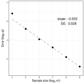
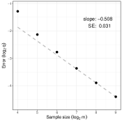
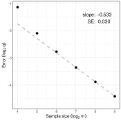
Number of replicates increasing

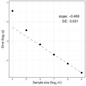
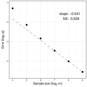
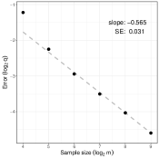
Figure 7: Like Figure 1, but with Pareto distributed data.

Figure 1 shows results for the case $n_{c}=m^{2}/8$ with normally distributed data. The horizontal axis is $m$ on a $\log_{2}$ scale and the vertical axis is the average value of $q$, also on a $\log_{2}$ scale. The dotted line is fitted to the final two points (when $m$ is $2^{8}$ and $2^{9}$), and its slope therefore gives an indication of how $q$ decays with $m$ asymptotically. This slope and its standard error are provided in each plot. We see that in all cases, $q$ tends to 0, and appears to do so at a $m^{-1/2}$ rate. This is true for both replication structures and even when $k$ is overestimated. A similar plot, Figure 7, is provided in the appendix for the Pareto case and the results are essentially the same.

	$k=3$	$k=10$	$k=k_{\mathrm{max}}$
Number of samples increasing
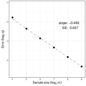
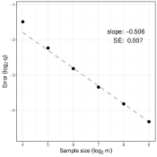
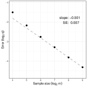
Number of replicates increasing

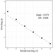
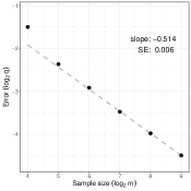
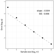
Figure 1: Simulation results for the case $n_{c}=m^{2}/8$ with normally distributed data.

Figure 2 compares the three cases of $n_{c}$. Interestingly, when $k=3$, the results are almost identical for all three cases, suggesting that we may obtain a good adjustment even with a fairly limited number of negative controls. However, when $k$ is overestimated, especially when $k=k_{\mathrm{max}}$, the quality of the adjustment is more sensitive to the number of negative controls. From a practical point of view, this suggests that when the number of negative controls is limited, extra attention should be given to the selection of $k$ (Gagnon-Bartsch and Speed, 2012; Molania et al., 2019, 2022). Nonetheless, we note that even when $n_{c}=2m$ and $k=k_{\mathrm{max}}$, it still appears that $q\to 0$, although not at a $m^{-1/2}$ rate.

$k=3$	$k=10$	$k=k_{\mathrm{max}}$

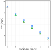
Figure 2: Simulation results comparing the cases $n_{c}=m^{2}/8$ (red circle), $n_{c}=m^{3/2}/2$ (green triangle), and $n_{c}=2m$ (blue square). Data is normally distributed, and samples increasing.

Figure 3 shows the same results as Figure 2, but arranged differently to more directly compare the impact of $k$. Of particular note are the left and center panels, which suggest that asymptotically there is effectively no penalty for overestimating $k$ when the number of negative controls is moderately large, relative to the sample size. However, at smaller sample sizes or with a limited number of negative controls the choice of $k$ has a modest impact.

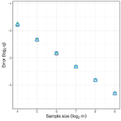
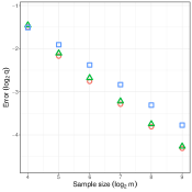
Figure 8: Like Figure 2, but with Pareto distributed data.

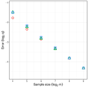
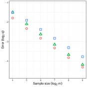
Figure 9: Like Figure 3, but with Pareto distributed data.

Figures 8 and 9 in the appendix are similar to Figures 2 and 3 but with the Pareto distribution, and look essentially the same.

$n_{c}=\frac{1}{8}m^{2}$	$n_{c}=\frac{1}{2}m^{\frac{3}{2}}$	$n_{c}=2m$

Figure 3: Simulation results comparing the cases $k=3$ (red circle), $k=10$ (green triangle), and $k=k_{\mathrm{max}}$ (blue square). Data is normally distributed, and samples increasing.

5.2 A real-data example

We apply RUV-III to a microarray dataset both to demonstrate the efficacy of RUV-III, as well as to highlight the role that negative controls and replicates can play in essentially defining what variation is wanted and what is unwanted.

We use the dataset of Vawter et al. (2004), which is the same dataset analyzed in Gagnon-Bartsch and Speed (2012). Briefly, the goal of the original study was to find genes differentially expressed in the brain with respect to sex. Tissue samples were collected post-mortem from 10 individuals, 5 male and 5 female. Three tissue samples were taken from each individual — one from the anterior cingulate cortex (ACC), one from the dorsolateral prefrontal cortex (DLPFC), and one from the cerebellum (CB). Thus, $10\times 3=30$ tissue samples were collected in total. Three aliquots were derived from each sample, and sent to three different laboratories for analysis (UC Davis, UC Irivine, U. Michigan); this was for sake of replication, and the analysis at each laboratory was in principle the same. In particular, each laboratory assayed their 30 aliquots on Affymetrix HG U95 microarrays, resulting in a total of $30\times 3=90$ microarray assays. Data from 6 of the 90 are unavailable, presumably due to quality control issues, so we only have a final sample size of $m=84$. Each microarray measures the gene expression of $n=12,600$ probesets (genes). 33 of these probesets correspond to spike-in controls, exogenous RNA added at a fixed concentration to each sample for quality control. For additional details, see Vawter et al. (2004) and Gagnon-Bartsch and Speed (2012).

In Figure 4, top-left panel, we plot the first two PCs of the data. We see that the primary clustering is by laboratory, indicating strong batch effects. Notably, these batch effects persist even though the data have been quantile normalized by RMA.

We now apply RUV-III as follows. As negative controls, we use the $n_{c}=33$ spike-in probesets. The mapping matrix is the $84\times 30$ matrix in which each column corresponds to a single tissue sample. We set $k=10$ as in Gagnon-Bartsch and Speed (2012). The results are shown in Figure 4, top-right panel. The laboratory batch effects have been removed, and the primary clustering is now by brain region; cerebellum forms one cluster, and the two types of cortex form the other cluster. Thus RUV-III has succeeded in its primary goal — it has removed unwanted technical variation while preserving biological variation.

No Adjustment	“Technical” Adjustment
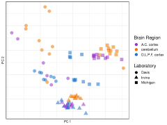
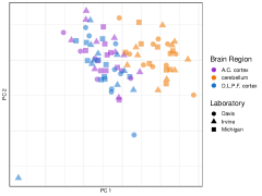
“Bio” Adjustment	“Bio” Adjustment (colored by patient)

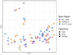
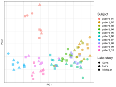
Figure 4: PC plots of the brain dataset before and after adjustment by RUV-III. The “technical” adjustment uses spike-in controls and define replicates purely as technical replicates (same sample but different lab). The “bio” adjustment uses housekeeping genes and defines to include all assays from a single individual.

One of the advantages of RUV-III is flexibility in the choice of negative controls and flexibility in the specification of replicates. This flexibility can be used to effectively define which sources of variation are wanted and which are unwanted. For example, although brain region effects might be of interest in some contexts, if the primary goal of the analysis is to find genes differentially expressed by sex, then we might wish to remove brain region effects in addition to batch effects.

In this spirit, we consider an alternative application of RUV-III. As negative controls, we use $n_{c}=799$ housekeeping genes (Eisenberg and Levanon, 2003). Housekeeping genes tend to have relatively stable expression, and we expect them to be negative controls with respect to sex. Nonetheless, even housekeeping genes may exhibit expression differences across tissue types, and we therefore expect some of these genes to capture brain region differences. As the mapping matrix we use the $84\times 10$ matrix in which each column corresponds to an individual person. Thus the “replicates” span the three tissue types, allowing us to capture tissue-type variation in $W$. On the other hand, since each set of replicates corresponds to one individual, the replicates should not capture sex differences.

The results are shown in Figure 4, bottom-left panel. Indeed, there is no longer clustering by brain region (nor by laboratory). The bottom-right panel of Figure 4 is the same plot but colored by individual. We see that now the assays cluster by person. Thus in this application of RUV-III we have preserved some sources of biological variation while removing others.

Figure 5 reveals how these adjustments impact a differential expression analysis. We regress each gene on sex and compute a p-value. A histogram of the 12,600 p-values should ideally be mostly flat, with a spike on the left corresponding to the genes that are truly differentially expressed. As seen in Figure 5, however, prior to RUV-III the p-value histogram is skewed to the right, with only a small spike on the left. After the “technical” adjustment, the p-value distribution is improved, and more so after the “bio” adjustment. In addition, we rank the genes by p-value, and check to see how many of the top-ranked genes lie on the sex chromosomes (X or Y). More specifically, for each value of $N$ from 1 to 50 we count the number of genes located on X or Y that are ranked in the top $N$ genes. The results are plotted on the right side of Figure 5, and we see that the “bio” adjustment substantially increases the number of top-ranked genes on the sex chromosomes. For example, before adjustment 15 of the 50 top-ranked genes are on the X or Y chromosome, but this increases to 24 after the “bio” adjustment. (For context, 488 of the 12,600 genes — fewer than 4% — lie on the X or Y chromosome.)

No Adjustment
“Technical” Adjustment
“Bio” Adjustment

Figure 5: P-value histograms (left) and rank plots (right) before and after RUV-III. Histogram break points are at 0.001, 0.01, 0.05, 0.1, 0.15, 0.2, …, 0.95.

To further investigate the ability of RUV-III to remove unwanted variation while preserving variation of interest, in Figure 6 we create PC plots similar to those of Figure 4, but using only genes from the sex chromosomes. (The application of RUV-III is exactly the same as in Figure 4; the only difference is which genes are used to calculate the PCs.) We expect many of these genes to be differentially expressed with respect to sex, and therefore might naturally expect males and females to form clusters on a PC plot. Panels (a) and (b) plot the first two PCs before adjustment. Perhaps surprisingly, we see that even when we focus on just the sex chromosomes, there is no clustering by male/female apparent in the first two PCs. In panel (a) we see that the strongest factor is still the laboratory batch effect, and in panel (b) we see that there is no discernible clustering by sex even within labs; the plusses and diamonds appear randomly distributed. Likewise, in panel (b) we see that the primary signal after the “technical” adjustment is still brain region. Again, although we have limited our PC analysis to X/Y genes, there is no discernible clustering by sex. In panel (d), however, after applying the “bio” adjustment, sex differences appear prominently in the first PC.

(a)	(b)
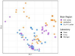
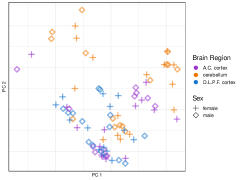
(c)	(d)

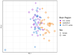
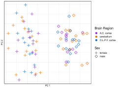
Figure 6: PC plots of X/Y genes before and after adjustment. (a) No adjustment. Like top-left panel of Figure 4, but with PCs computed only on X/Y genes. (b) No adjustment. Like panel (a), but plot symbol denotes sex. (c) “Technical” Adjustment. Like panel (b), but after RUV-III technical adjustment. (d) “Bio” Adjustment. Like panel (b), but after RUV-III bio adjustment.

We emphasize that this example is not intended to suggest intrinsic superiority of housekeeping genes over spike-in controls, or of using biological replicates over technical replicates. Rather, we emphasize that the choice of negative controls and the specification of what constitutes a replicate plays a critical role in determining which variation is captured and removed by RUV-III and which variation is preserved.

6 Acknowledgement

TPS would like to thank the Institute of Mathematical Sciences of the National University of Singapore for the invitation to speak at their January 2022 Workshop on Statistical Methods in Genetic/Genomic Studies at which a rudimentary version of the ideas in this paper were presented. Jiming Jiang’s research was supported by the National Science Foundation of the United States grant DMS-1713120.

7 Code and Data

Code and data are available at https://github.com/johanngb/ruvIIItheory and a Docker image is available at https://osf.io/yhvna/.

8 Proofs

Throughout the proofs, $L_{r}$ denotes a generic matrix satisfying $\|L_{r}\|=o(\|W\alpha\|^{r})$, $r=1,2$. We use w. p. $\rightarrow 1$ for “with probability tending to one”.

8.1 Proof of Theorem 1

Assumption (I) implies $1\leq k\leq m-s$ w. p. $\rightarrow 1$. We have

$$P_{1^{\perp}}Y_{\rm c} = W\alpha_{\rm c}+P_{1^{\perp}}\epsilon_{\rm c},$$ (44)

$$U_{(k)}^{\prime}Y_{\rm c} = U_{(k)}^{\prime}W\alpha_{\rm c}+U_{(k)}^{\prime}\epsilon_{\rm c},$$ (45)

$$\hat{\alpha}_{(k)} = U_{(k)}^{\prime}W\alpha+U_{(k)}^{\prime}\epsilon,$$ (46)

For (45), note that, by (1), we have

$$P_{M} = {\rm diag}(1_{m_{h}},1\leq h\leq s){\rm diag}(m_{h}^{-1},1\leq h\leq s){\rm diag}(1_{m_{h}}^{\prime},1\leq h\leq s)$$ (47)

$$= {\rm diag}(P_{1_{m_{h}}},1\leq h\leq s),$$

where $P_{1_{d}}=d^{-1}1_{d}1_{d}^{\prime}$. It then follows that $P_{M^{\perp}}1=0$. Also, identity (14) implies

$$0=P_{M^{\perp}}YY^{\prime}P_{M^{\perp}}1=\sum_{l=1}^{m-s}\lambda_{l}u_{l}u_{l}^{\prime}1.$$ (48)

The assumptions imply (see the arguments below) that $\lambda_{j}>0,1\leq j\leq k$ w. p. $\rightarrow 1$. For any $1\leq j\leq k$, by the orthonormality of the $u_{l}$’s, we have [by multiplying $u_{j}^{\prime}$ from the left on both sizes of (48)], $\lambda_{j}u_{j}^{\prime}1=0$; then, because $\lambda_{j}>0$, we have $u_{j}^{\prime}1=0$, and this holds for any $1\leq j\leq k$, implying $U_{(k)}^{\prime}1=0$. Similarly, it can be shown that $U_{(k)}^{\prime}M=0$, leading to (46).

We now establish (8). We use the following notation: Define $A_{\rm c}$, $B$, $G$ and $H$ as below (9). Let $\xi=U_{(k)}^{\prime}\epsilon$, $\xi_{\rm c}=U_{(k)}^{\prime}\epsilon_{\rm c}$, $\eta_{\rm c}=P_{1^{\perp}}\epsilon_{\rm c}$; then let $\Delta_{1}=B\alpha_{\rm c}\xi_{\rm c}^{\prime}$, $\Delta_{2}=\xi_{\rm c}\xi_{\rm c}^{\prime}$, $\Delta=\Delta_{1}+\Delta_{1}^{\prime}+\Delta_{2}$; $\Gamma_{1}=W\alpha_{\rm c}\xi_{\rm c}^{\prime}$, $\Gamma_{2}=\eta_{\rm c}\alpha_{\rm c}^{\prime}B^{\prime}$, $\Gamma_{3}=\eta_{\rm c}\xi_{\rm c}^{\prime}$, $\Gamma=\Gamma_{1}+\Gamma_{2}+\Gamma_{3}$. By (5), (44)–(46), it can be shown that $U_{(k)}^{\prime}Y_{\rm c}Y_{\rm c}^{\prime}U_{(k)}=G+\Delta$, $P_{1^{\perp}}Y_{\rm c}Y_{\rm c}^{\prime}U_{(k)}=H+\Gamma$, thus, we have

$$\hat{W}_{(k)}=HG^{-1}(I_{k}+\Delta G^{-1})^{-1}+\Gamma G^{-1}(I_{k}+\Delta G^{-1})^{-1}.$$

Thus, it can be verified that (8) holds with $T_{1}=HG^{-1}(Q-I_{k})B\alpha$, $T_{2}=\Gamma G^{-1}QB\alpha$, $T_{3}=HG^{-1}Q\xi$, $T_{4}=\Gamma G^{-1}Q\xi$, where $Q=(I_{k}+\Delta G^{-1})^{-1}$.

It remains to show that all of the terms $T_{s},s=1,2,3,4$ are $L_{1}$ (see notation at the beginning of this section). A main task is working on $G$. Write

$$G = U_{(k)}^{\prime}W\alpha_{\rm c}\alpha_{\rm c}^{\prime}W^{\prime}U_{(k)}$$ (49)

$$= n_{\rm c}U_{(k)}^{\prime}W\Sigma W^{\prime}U_{(k)}+n_{\rm c}U_{(k)}^{\prime}W(n_{\rm c}^{-1}\alpha_{\rm c}\alpha_{\rm c}^{\prime}-\Sigma)W^{\prime}U_{(k)}.$$

Assumption (II) implies $n_{\rm c}^{-1}\alpha_{\rm c}\alpha_{\rm c}^{\prime}-\Sigma=n_{\rm c}^{-1}\sum_{j=1}^{n_{\rm c}}(\alpha_{j}\alpha_{j}^{\prime}-\Sigma)=O_{\rm P}(1)/\sqrt{n_{\rm c}}$. Furthermore, (6) implies $\|W\|^{2}=\lambda_{m}O(1)$, hence $\|U_{(k)}^{\prime}W(n_{\rm c}^{-1}\alpha_{\rm c}\alpha_{\rm c}^{\prime}-\Sigma)W^{\prime}U_{(k)}\|\leq(\lambda_{m}/\sqrt{n_{\rm c}})O_{\rm P}(1)$. It then follows, by (49), that we can write

$$G=n_{\rm c}U_{(k)}^{\prime}W\Sigma W^{\prime}U_{(k)}+\lambda_{m}\sqrt{n_{\rm c}}O_{\rm P}(1).$$ (50)

On the other hand, because $P_{M^{\perp}}Y=P_{M^{\perp}}(W\alpha+\epsilon)$, we have

$$P_{M^{\perp}}YY^{\prime}P_{M^{\perp}} = P_{M^{\perp}}W\alpha\alpha^{\prime}W^{\prime}P_{M^{\perp}}+P_{M^{\perp}}(\epsilon\epsilon^{\prime}+\epsilon\alpha^{\prime}W^{\prime}+W\alpha\epsilon^{\prime})P_{M^{\perp}}$$ (51)

$$= nP_{M^{\perp}}W\Sigma W^{\prime}P_{M^{\perp}}+nP_{M^{\perp}}W(n^{-1}\alpha\alpha^{\prime}-\Sigma)W^{\prime}P_{M^{\perp}}$$

$$+P_{M^{\perp}}(\epsilon\epsilon^{\prime}+\epsilon\alpha^{\prime}W^{\prime}+W\alpha\epsilon^{\prime})P_{M^{\perp}}.$$

By similar arguments, the second term on the right side of (51) is $\lambda_{m}\sqrt{n}O_{\rm P}(1)$. Furthermore, note that $\|P_{M^{\perp}}\|\leq 1$, $\|\epsilon\|=\sqrt{n}O_{\rm P}(1)$ by the RMT (e.g., (Jiang, 2022), ch. 16); also, it can be shown that $\|\alpha\|=\sqrt{n}O_{\rm P}(1)$. It follows that the third term on the right side of (51) is $n\sqrt{\lambda_{m}}O_{\rm P}(1)$. Note that $U_{(k)}^{\prime}P_{M^{\perp}}YY^{\prime}P_{M^{\perp}}U_{(k)}=[u_{g}^{\prime}P_{M^{\perp}}YY^{\prime}P_{M^{\perp}}u_{h}]_{1\leq g,h\leq k}$. Thus, assuming $k\leq m-s$, which holds w. p. $\rightarrow 1$, we have, by (14), $u_{g}^{\prime}P_{M^{\perp}}YY^{\prime}P_{M^{\perp}}u_{h}=\sum_{l=1}^{m-s}\lambda_{l}u_{g}^{\prime}u_{l}u_{l}^{\prime}u_{h}$, which is $0$ if $g\neq h$; if $g=h$, the expression is equal to $\lambda_{g}$. Thus, combining the above results, we have

$$\lambda_{k}I_{k} \leq {\rm diag}(\lambda_{1},\dots,\lambda_{k})$$ (52)

$$= U_{(k)}^{\prime}P_{M^{\perp}}YY^{\prime}P_{M^{\perp}}U_{(k)}$$

$$= nU_{(k)}^{\prime}W\Sigma W^{\prime}U_{(k)}+(\lambda_{m}\sqrt{n}+n\sqrt{\lambda_{m}})O_{\rm P}(1),$$

noting that $P_{M^{\perp}}U_{(k)}=U_{(k)}$ and $\|U_{(k)}\|=1$. Combining (50) and (52), we have

$$G = \left(\frac{n_{\rm c}}{n}\right)nU_{(k)}^{\prime}W\Sigma W^{\prime}U_{(k)}+\lambda_{m}\sqrt{n_{\rm c}}O_{\rm P}(1)$$ (53)

$$\geq \left(\frac{n_{\rm c}}{n}\right)\{\lambda_{k}I_{k}-(\lambda_{m}\sqrt{n}+n\sqrt{\lambda_{m}})O_{\rm P}(1)\}+\lambda_{m}\sqrt{n_{\rm c}}O_{\rm P}(1)$$

$$= \lambda_{k}\left(\frac{n_{\rm c}}{n}\right)I_{k}-(\lambda_{m}\sqrt{n}+n\sqrt{\lambda_{m}})O_{\rm P}(1).$$

We now utilize a result from the eigenvalue perturbation theory. For any $m\times m$ symmetric matrix $A$, let $\lambda_{1}(A)\geq\cdots\geq\lambda_{m}(A)$ denote its eigenvalues arranged in decreasing order. We have the following inequality (e.g., (Jiang, 2022), p. 156).

Lemma 1 (Weyl’s eigenvalue perturbation theorem). For any symmetric matrices $A,B$, we have $\max_{1\leq i\leq m}|\lambda_{i}(A)-\lambda_{i}(B)|\leq\|A-B\|$.

Now $\lambda_{1},\dots,\lambda_{m}$ are the eigenvalues of $P_{M^{\perp}}YY^{\prime}P_{M^{\perp}}$ arranged in decreasing order. Let $\gamma_{1},\dots,\gamma_{m}$ denote the eigenvalues of $F_{M}=P_{M^{\perp}}W\alpha\alpha^{\prime}W^{\prime}P_{M^{\perp}}$, also arranged in decreasing order. Then, by Lemma 1 and (51), we have

$$\max_{1\leq i\leq k}|\lambda_{i}-\gamma_{i}|\leq\|P_{M^{\perp}}(\epsilon\epsilon^{\prime}+\epsilon\alpha^{\prime}W^{\prime}+W\alpha\epsilon^{\prime})P_{M^{\perp}}\|=n\sqrt{\lambda_{m}}O_{\rm P}(1).$$ (54)

Next, we have $F_{M}=nP_{M^{\perp}}W(n^{-1}\alpha\alpha^{\prime})W^{\prime}P_{M^{\perp}}=nJ_{M}+nP_{M^{\perp}}W(n^{-1}\alpha\alpha^{\prime}-\Sigma)W^{\prime}P_{M^{\perp}}$, where $J_{M}=P_{M^{\perp}}W\Sigma W^{\prime}P_{M^{\perp}}$. Let $\rho_{1},\dots,\rho_{m}$ denote the eigenvalues of $J_{M}$, arranged in decreasing order. Then, again, by Lemma 1, we have

$$\max_{1\leq i\leq k}|\gamma_{i}-n\rho_{i}|\leq n\|P_{M^{\perp}}W(n^{-1}\alpha\alpha^{\prime}-\Sigma)W^{\prime}P_{M^{\perp}}\|=\lambda_{m}\sqrt{n}O_{\rm P}(1).$$ (55)

Note that $J_{M}$ is $m\times m$. Thus, assuming ${\rm rank}(J_{M})\geq k$, which holds w. p. $\rightarrow 1$ under the assumptions, we have $\rho_{k}\geq$ the smallest nonzero eigenvalue of $J_{M}$, which is the same as the smallest eigenvalue of $\Sigma^{1/2}W^{\prime}P_{M^{\perp}}W\Sigma^{1/2}$, provided that the latter, which is $k\times k$, is positive definite, which again holds w. p. $\rightarrow 1$ under the assumptions. It can be shown that $W^{\prime}P_{M^{\perp}}W=\sum_{h=1}^{s}(W_{h}-1_{m_{h}}\bar{W}_{h}^{\prime})^{\prime}(W_{h}-1_{m_{h}}\bar{W}_{h}^{\prime})$. Thus, we have $\rho_{k}\geq\lambda_{\min}(W^{\prime}P_{M^{\perp}}W)\lambda_{\min}(\Sigma)=\lambda_{\min}(\Sigma)\lambda_{m}$. Note that $\rho_{k}>0$ implies ${\rm rank}(J_{M})=k$. Combining the above results, we have obtained a asymptotic lower bound for $\lambda_{k}$:

$$\lambda_{k} = n\rho_{k}+\lambda_{k}-n\rho_{k}$$ (56)

$$\geq n\lambda_{m}\lambda_{\min}(\Sigma)-\max_{1\leq i\leq k}|\lambda_{i}-n\rho_{i}|$$

$$\geq \lambda_{m}n\left\{\lambda_{\min}(\Sigma)-\frac{O_{\rm P}(1)}{\sqrt{\lambda_{m}}}-\frac{O_{\rm P}(1)}{\sqrt{n}}\right\}.$$

Combining (53) and (56), we have

$$G \geq \left(\frac{n_{\rm c}}{n}\right)\lambda_{m}n\left\{\lambda_{\min}(\Sigma)-\frac{O_{\rm P}(1)}{\sqrt{\lambda_{m}}}-\frac{O_{\rm P}(1)}{\sqrt{n}}\right\}I_{k}-(\lambda_{m}\sqrt{n}+n\sqrt{\lambda_{m}})O_{\rm P}(1)$$ (57)

$$= \lambda_{m}n\left[\left(\frac{n_{\rm c}}{n}\right)\left\{\lambda_{\min}(\Sigma)-\frac{O_{\rm P}(1)}{\sqrt{\lambda_{m}}}-\frac{O_{\rm P}(1)}{\sqrt{n}}\right\}I_{k}-\frac{O_{\rm P}(1)}{\sqrt{n}}-\frac{O_{\rm P}(1)}{\sqrt{\lambda_{m}}}\right]$$

$$= \lambda_{m}n\left[\left(\frac{n_{\rm c}}{n}\right)\lambda_{\min}(\Sigma)I_{k}-\frac{O_{\rm P}(1)}{\sqrt{\lambda_{m}}}-\frac{O_{\rm P}(1)}{\sqrt{n}}\right].$$

It then follows, by assumption (I), that we have the following key result:

$$G^{-1}=(\lambda_{m}n)^{-1}O_{\rm P}(1).$$ (58)

Also, we have $\Delta_{1}=U_{(k)}^{\prime}W\alpha\epsilon^{\prime}U_{(k)}=U_{(k)}^{\prime}P_{M^{\perp}}W\alpha\epsilon^{\prime}U_{(k)}$, hence $|\Delta_{1}|\leq\|P_{M^{\perp}}W\alpha\epsilon^{\prime}\|$. We have $\|P_{M^{\perp}}\|=\sqrt{\lambda_{m}}O(1)$ by (6); $\|\alpha\|=\sqrt{n}O_{\rm P}(1)$ by assumption (II); and $\|\epsilon\|=\sqrt{n}O_{\rm P}(1)$ by assumption (III) and the RMT. It follows that $|\Delta_{1}|=\sqrt{\lambda_{m}}nO_{\rm P}(1)$. Similarly, it can be shown that $|\Delta_{2}|=nO_{\rm P}(1)$. Thus, we have $|\Delta|=\sqrt{\lambda_{m}}nO_{\rm P}(1)$, hence $\Delta G^{-1}=O_{\rm P}(1)/\sqrt{\lambda_{m}}=o_{\rm P}(1)$ by (58), assumption (I) and (7), hence $Q-I_{k}=O_{\rm P}(1)/\sqrt{\lambda_{m}}$.

Note that $T_{1}=HG^{-1}(Q-I_{k})U_{(k)}^{\prime}W\alpha$, and $H=W\alpha_{\rm c}\alpha_{\rm c}^{\prime}W^{\prime}P_{M^{\perp}}U_{(k)}$. Thus, we have

$$|H|\leq\|W\alpha_{\rm c}\|\sqrt{U_{(k)}^{\prime}P_{M^{\perp}}W\alpha_{\rm c}\alpha_{\rm c}^{\prime}W^{\prime}P_{M^{\perp}}U_{(k)}}=\lambda_{m}n_{\rm c}O_{\rm P}(1),$$

which is implied by the assumptions [in particular, (7)]. It follows that

$$\|HG^{-1}(Q-I_{k})U_{(k)}^{\prime}\|\leq\lambda_{m}n_{\rm c}O_{\rm P}(1)\left\{\frac{O_{\rm P}(1)}{\lambda_{m}n}\right\}\left\{\frac{O_{\rm P}(1)}{\sqrt{\lambda_{m}}}\right\}\leq\frac{O_{\rm P}(1)}{\sqrt{\lambda_{m}}}.$$

Thus, by (7), we have $T_{1}=o_{\rm P}(1)W\alpha=L_{1}$ (see notation at the beginning of this section).

Next, by (58), we have $T_{2}=\Gamma\{(\lambda_{m}n)^{-1}O_{\rm P}(1)\}U_{(k)}^{\prime}W\alpha$. By similar arguments, it can be shown that $\|\Gamma\|=\sqrt{\lambda_{m}}nO_{\rm P}(1)$, and $\|U_{(k)}\|=1$. Thus, we have $T_{2}=o_{\rm P}(1)W\alpha=L_{1}$.

As for $T_{j},j=3,4$, we first obtain an asymptotic lower bound for $\|W\alpha\|$. By the following inequalities (e.g., Ex. 5.27 of (Jiang, 2022) 2022):

$$\lambda_{\max}(A)+\lambda_{\min}(B)\leq\lambda_{\max}(A+B)\leq\lambda_{\max}(A)+\lambda_{\max}(B)$$

for matrices $A,B$ of same dimensions, and the arguments above, it can be shown that

$$\left|\|W\alpha\|^{2}-n\lambda_{\max}(W\Sigma W^{\prime})\right|\leq\lambda_{m}\sqrt{n}O_{\rm P}(1).$$

Furthermore, using the fact that $W^{\prime}W\geq\lambda_{\min}(W^{\prime}W)I_{k}$ and some known matrix inequalities [e.g., (ii), (iii) of (Jiang, 2022), sec. 5.3.1], we have

$$\lambda_{\max}(W\Sigma W^{\prime})=\lambda_{\max}(\Sigma^{1/2}W^{\prime}W\Sigma^{1/2})\geq\lambda_{\min}(W^{\prime}W)\lambda_{\max}(\Sigma)$$

$$\geq\lambda_{\min}(W^{\prime}P_{M^{\perp}}W)\lambda_{\max}(\Sigma)=\lambda_{\max}(\Sigma)\lambda_{m}.$$

It follows that, w. p. $\rightarrow 1$, $\|W\alpha\|/\sqrt{\lambda_{m}n}$ has a positive lower bound. On the other hand, it can be shown that, under assumptions (II) and (III), and (6), one has $\|T_{3}\|=\sqrt{n}O_{\rm P}(1)$, and $\|T_{4}\|=\sqrt{n/\lambda_{m}}O_{\rm P}(1)$. Therefore, by (7), both $T_{3}$ and $T_{4}$ are $L_{1}$.

The proof is complete by (8) and Definition 1 in Section 2.

8.2 Proof of Theorem 2

First, let us obtain a lower bound for the difference between the right side of (11), denoted by $g(k)$, and its maximum, $g(k_{0})$. We have

$$g(k_{0})-g_{(}k)=n{\rm tr}\{W\Sigma^{1/2}P_{\perp}(k)\Sigma^{1/2}W^{\prime}\},$$ (59)

where $P_{\perp}(k)=I_{k_{0}}-\Sigma^{1/2}B^{\prime}(B\Sigma B^{\prime})^{-1}B\Sigma^{1/2}$ is a projection matrix. Thus, we have

$${\rm tr}\{W\Sigma^{1/2}P_{\perp}(k)\Sigma^{1/2}W^{\prime}\} = {\rm tr}\{P_{\perp}(k)\Sigma^{1/2}W^{\prime}W\Sigma^{1/2}P_{\perp}(k)\}$$ (60)

$$\geq \lambda_{\min}(W^{\prime}W){\rm tr}\{P_{\perp}(k)\Sigma P_{\perp}(k)\}$$

$$\geq \lambda_{\min}(W^{\prime}P_{M^{\perp}}W)\lambda_{\min}(\Sigma){\rm tr}\{P_{\perp}(k)\}$$

$$= \lambda_{\min}(\Sigma)(k_{0}-k)\lambda_{m}.$$

Thus, under (6), the right side of (60) has an asymptotic lower bound, $a_{1}\lambda_{\min}(\Sigma)(k_{0}-k)\lambda_{m}$, for some constant $a_{1}>0$. It follows that the right side of (59) has an asymptotic lower bound, which is $a_{1}\lambda_{\min}(\Sigma)(k_{0}-k)\lambda_{m}n$.

Next, consider the difference between the right sides of (10) and (11). It can be shown that the difference can be written as $\sum_{s=1}^{5}d_{s}$, where

$$d_{1} = {\rm tr}[\{(BA_{\rm c}B^{\prime})^{-1}-(Bn_{\rm c}\Sigma B^{\prime})^{-1}\}BA_{\rm c}W^{\prime}WA_{\rm c}B^{\prime}(BA_{\rm c}B^{\prime})^{-1}B\alpha\alpha^{\prime}B^{\prime}],$$

$$d_{2} = {\rm tr}\{(Bn_{\rm c}\Sigma B^{\prime})^{-1}B(A_{\rm c}-n_{\rm c}\Sigma)W^{\prime}WA_{\rm c}B^{\prime}(BA_{\rm c}B^{\prime})^{-1}B\alpha\alpha^{\prime}B^{\prime}\},$$

$$d_{3} = {\rm tr}\{(Bn_{\rm c}\Sigma B^{\prime})^{-1}Bn_{\rm c}\Sigma W^{\prime}W(A_{\rm c}-n_{\rm c}\Sigma)B^{\prime}(BA_{\rm c}B^{\prime})^{-1}B\alpha\alpha^{\prime}B^{\prime}\},$$

$$d_{4} = {\rm tr}[(Bn_{\rm c}\Sigma B^{\prime})^{-1}Bn_{\rm c}\Sigma W^{\prime}Wn_{\rm c}\Sigma B^{\prime}\{(BA_{\rm c}B^{\prime})^{-1}-(Bn_{\rm c}\Sigma B^{\prime})^{-1}\}B\alpha\alpha^{\prime}B^{\prime}],$$

$$d_{5} = {\rm tr}\{(Bn_{\rm c}\Sigma B^{\prime})^{-1}Bn_{\rm c}\Sigma W^{\prime}Wn_{\rm c}\Sigma B^{\prime}(Bn_{\rm c}\Sigma B^{\prime})^{-1}B(\alpha\alpha^{\prime}-n\Sigma)B^{\prime}\}.$$

By the previous arguments [in particular, (50) and (58)], it can be shown that

$$d_{j}=\lambda_{m}no_{\rm P}(1),\;\;j=1,2,3,4,5.$$ (61)

By similar arguments, it can be also shown that

$$\|T_{j}\|_{2}^{2}=\lambda_{m}no_{\rm P}(1),\;\;j=1,2,3,4$$ (62)

for the $T_{j}$ in (9). It follows, by (9) and the Cauchy-Schwarz inequality that

$$\|\hat{W}_{(k)}\hat{\alpha}_{(k)}\|_{2}^{2}=\|HG^{-1}B\alpha\|_{2}^{2}+\lambda_{m}no_{\rm P}(1),$$ (63)

Combining (10), (11), and the above results, we have, w. p. $\rightarrow 1$,

$$\min_{1\leq k<k_{0}}\left\{\|\hat{W}_{(k_{0})}\hat{\alpha}_{(k_{0})}\|_{2}^{2}-\|\hat{W}_{(k)}\hat{\alpha}_{(k)}\|_{2}^{2}\right\}\geq\frac{a_{1}}{2}\lambda_{\min}(\Sigma)\lambda_{m}n;$$ (64)

in other words, (13) holds with $\delta_{1}=a_{1}/2$.

8.3 Proof of Theorem 3

First, let us continue on with the special case of $n=n_{\rm c}$, discussed in the early part of Section 3.2. By (16), we have

$$\hat{W}_{(k)}\hat{\alpha}_{(k)}=P_{1^{\perp}}Y_{\rm c}P=P_{1^{\perp}}Y_{\rm c}P_{0}+P_{1^{\perp}}Y_{\rm c}P_{+}.$$ (65)

We have $P_{1^{\perp}}Y_{\rm c}=P_{1^{\perp}}W\alpha+P_{1^{\perp}}\epsilon=W\alpha+L_{1}$, because $\|P_{1^{\perp}}\epsilon\|\leq\|\epsilon\|=\sqrt{n}O_{\rm P}(1)$ by the RMT. Thus (using the Cauchy-Schwarz inequality for the cross products), we have

$$P_{1^{\perp}}Y_{\rm c}PY_{\rm c}^{\prime}P_{1^{\perp}}=(W\alpha+L_{1})P(\alpha^{\prime}W^{\prime}+L_{1}^{\prime})$$

$$=W\alpha P\alpha^{\prime}W^{\prime}+L_{2}\leq W\alpha\alpha^{\prime}W^{\prime}+L_{2}$$ (66)

(see notation introduced at the beginning of Section 6). Furthermore, according to the proof of Theorem 1, we have $P_{1^{\perp}}Y_{\rm c}P_{0}=W\alpha+L_{1}$. Thus, we have

$$(P_{1^{\perp}}Y_{\rm c}P_{0}+P_{1^{\perp}}Y_{\rm c}P_{+})(P_{0}Y_{\rm c}^{\prime}P_{1^{\perp}}+P_{+}Y_{\rm c}^{\prime}P_{1^{\perp}})$$ (67)

$$= P_{1^{\perp}}Y_{\rm c}P_{0}Y_{\rm c}^{\prime}P_{1^{\perp}}+P_{1^{\perp}}Y_{\rm c}P_{+}Y_{\rm c}^{\prime}P_{1^{\perp}}$$

$$= (W\alpha+L_{1})(\alpha^{\prime}W^{\prime}+L_{1}^{\prime})+P_{1^{\perp}}Y_{\rm c}P_{+}Y_{\rm c}^{\prime}P_{1^{\perp}}$$

$$= W\alpha\alpha^{\prime}W^{\prime}+L_{2}+P_{1^{\perp}}Y_{\rm c}P_{+}Y_{\rm c}^{\prime}P_{1^{\perp}},$$

using the fact that $P_{0}P_{+}=P_{+}P_{0}=0$ and, again, the Cauchy-Schwarz inequality for the cross products. Combining the second equation in (65), (66), and (67), we have $W\alpha\alpha^{\prime}W^{\prime}+L_{2}+P_{1^{\perp}}Y_{\rm c}P_{+}Y_{\rm c}^{\prime}P_{1^{\perp}}\leq W\alpha\alpha^{\prime}W^{\prime}+L_{2}$, hence $P_{1^{\perp}}Y_{\rm c}P_{+}Y_{\rm c}^{\prime}P_{1^{\perp}}\leq L_{2}$, which implies $P_{1^{\perp}}Y_{\rm c}P_{+}=L_{1}$. Thus, by (65) and combining the above results, we have established that

$$\hat{W}_{(k)}\hat{\alpha}_{(k)}=W\alpha+L_{1}$$ (68)

for every fixed $k_{0}<k\leq K$, where $K$ is the maximum number of $k$ under consideration.

It is worth noting that, in fact, the arguments of the above proof apply to any fixed sequence of $k$, say, $k=k_{N}$, which $N$ denotes the combination of $m,n,n_{\rm c}$, etc. that may increase, such that $k_{N}\leq m-s$ and $k_{N}\rightarrow\infty$. In particular, the arguments apply to $k_{N}=m-s$.

Now let us remove the $n=n_{\rm c}$ assumption. In this case, $U_{(k)}^{\prime}Y_{\rm c}Y_{\rm c}^{\prime}U_{(k)}$ is not necessarily block-diagonal. However, by the inversion of blocked matrices (e.g., (Bernstein, 2009) p.44), we have

$$\{U_{(k)}^{\prime}Y_{\rm c}Y_{\rm c}^{\prime}U_{(k)}\}^{-1}$$

$$= \left[\begin{array}[]{cc}U_{(k_{0})}^{\prime}Y_{\rm c}Y_{\rm c}^{\prime}U_{(k_{0})}&U_{(k_{0})}^{\prime}Y_{\rm c}Y_{\rm c}^{\prime}U_{(+)}\\ U_{(+)}^{\prime}Y_{\rm c}Y_{\rm c}^{\prime}U_{(k_{0})}&U_{(+)}^{\prime}Y_{\rm c}Y_{\rm c}^{\prime}U_{(+)}\end{array}\right]^{-1}$$

$$= {\footnotesize\left[\begin{array}[]{cc}Q_{00}^{-1}+Q_{00}^{-1}Q_{0+}\{U_{(+)}^{\prime}Y_{\rm c}P_{0}^{\perp}Y_{\rm c}^{\prime}U_{(+)}\}^{-1}Q_{+0}Q_{00}^{-1}&-Q_{00}^{-1}Q_{0+}\{U_{(+)}^{\prime}Y_{\rm c}P_{0}^{\perp}Y_{\rm c}^{\prime}U_{(+)}\}^{-1}\\ -\{U_{(+)}^{\prime}Y_{\rm c}P_{0}^{\perp}Y_{\rm c}^{\prime}U_{(+)}\}^{-1}Q_{+0}Q_{00}^{-1}&\{U_{(+)}^{\prime}Y_{\rm c}P_{0}^{\perp}Y_{\rm c}^{\prime}U_{(+)}\}^{-1}\end{array}\right]},$$

where $Q_{00}=U_{(k_{0})}^{\prime}Y_{\rm c}Y_{\rm c}^{\prime}U_{(k_{0})}$, $Q_{0+}=U_{(k_{0})}^{\prime}Y_{\rm c}Y_{\rm c}^{\prime}U_{(+)}$, $Q_{+0}=Q_{0+}^{\prime}$, and $P_{0}^{\perp}=I_{n_{\rm c}}-P_{0}$ with $P_{0}$ defined above. Also retain the notation $P$ previously define. It follows that

$$P = P_{0}+Y_{\rm c}^{\prime}U_{(k_{0})}Q_{00}^{-1}Q_{0+}\{U_{(+)}^{\prime}Y_{\rm c}P_{0}^{\perp}Y_{\rm c}^{\prime}U_{(+)}\}^{-1}Q_{+0}Q_{00}^{-1}U_{(k_{0})}^{\prime}Y_{\rm c}$$ (71)

$$-Y_{\rm c}^{\prime}U_{(+)}\{U_{(+)}^{\prime}Y_{\rm c}P_{0}^{\perp}Y_{\rm c}^{\prime}U_{(+)}\}^{-1}Q_{+0}Q_{00}^{-1}U_{(k_{0})}^{\prime}Y_{\rm c}$$

$$-Y_{\rm c}^{\prime}U_{(k_{0})}Q_{00}^{-1}Q_{0+}\{U_{(+)}^{\prime}Y_{\rm c}P_{0}^{\perp}Y_{\rm c}^{\prime}U_{(+)}\}^{-1}U_{(+)}^{\prime}Y_{\rm c}$$

$$+Y_{\rm c}^{\prime}U_{(+)}\{U_{(+)}^{\prime}Y_{\rm c}P_{0}^{\perp}Y_{\rm c}^{\prime}U_{(+)}\}^{-1}U_{(+)}^{\prime}Y_{\rm c}$$

$$= P_{0}+Y_{\rm c}^{\prime}\Lambda\{U_{(+)}^{\prime}Y_{\rm c}P_{0}^{\perp}Y_{\rm c}^{\prime}U_{(+)}\}^{-1}\Lambda^{\prime}Y_{\rm c}$$

$$= P_{0}+P_{\Lambda}$$

where $\Lambda=U_{(+)}-U_{(k_{0})}Q_{00}^{-1}Q_{0+}$ and $P_{\Lambda}=P_{Y_{\rm c}^{\prime}\Lambda}$. Note that $U_{(+)}^{\prime}Y_{\rm c}P_{0}^{\perp}Y_{\rm c}^{\prime}U_{(+)}=\Lambda^{\prime}Y_{\rm c}Y_{\rm c}^{\prime}\Lambda$. Also note that $U_{(k_{0})}^{\prime}Y_{\rm c}Y_{\rm c}^{\prime}\Lambda=0$, which implies $P_{0}P_{\Lambda}=0$. Furthermore, by the previous argument, we have $P_{1^{\perp}}Y_{\rm c}P_{0}=W\alpha_{\rm c}+L_{1}$. Thus, by similar argument to (67), we have

$$P_{1^{\perp}}Y_{\rm c}PY_{\rm c}^{\prime}P_{1^{\perp}}=W\alpha_{\rm c}\alpha_{\rm c}^{\prime}W^{\prime}+L_{2}+P_{1^{\perp}}Y_{\rm c}P_{\Lambda}Y_{\rm c}^{\prime}P_{1^{\perp}}.$$ (72)

On the other hand, by similar argument to (66), we have

$$P_{1^{\perp}}Y_{\rm c}PY_{\rm c}^{\prime}P_{1^{\perp}}\leq W\alpha_{\rm c}\alpha_{\rm c}^{\prime}W+L_{2}.$$ (73)

Combining (72) and (73), we have $0\leq P_{1^{\perp}}Y_{\rm c}P_{\Lambda}Y_{\rm c}^{\prime}P_{1^{\perp}}\leq L_{2}$, from which, it follows that $P_{1^{\perp}}Y_{\rm c}P_{\Lambda}=L_{1}$. Thus, combining the above results, we have

$$P_{1^{\perp}}Y_{\rm c}P=W\alpha_{\rm c}+L_{1}.$$ (74)

Next, similar to (71), we have the following expression:

$$Q=Q_{0}+Q_{\Lambda},$$ (75)

where the $Q$’s are the corresponding $P$’s with the last multiplication factor, $Y_{\rm c}$, replaced by $Y_{\rm d}$, and $Y=(Y_{\rm c}\;Y_{\rm d})$. Note that the $Y_{\rm d}$ in $Q_{\Lambda}$ can be replaced by $\xi_{\rm d}$ [because $U_{(k)}^{\prime}1=0$ and $U_{(k)}^{\prime}M=0$ for every $1\leq k\leq m-s$; see below (47) and (48)]. Thus, we have

$$P_{1^{\perp}}Y_{\rm c}Q_{\Lambda}Q_{\Lambda}^{\prime}Y_{\rm c}^{\prime}P_{1^{\perp}}$$

$$= P_{1^{\perp}}Y_{\rm c}Y_{\rm c}^{\prime}\Lambda(\Lambda^{\prime}Y_{\rm c}Y_{\rm c}^{\prime}\Lambda)^{-1}\Lambda^{\prime}\xi_{\rm d}\xi_{\rm d}^{\prime}\Lambda(\Lambda^{\prime}Y_{\rm c}Y_{\rm c}^{\prime}\Lambda)^{-1}Y_{\rm c}Y_{\rm c}^{\prime}P_{1^{\perp}}$$

$$= P_{1^{\perp}}\cdots\Lambda^{\prime}(\xi_{\rm c}\xi_{\rm c}^{\prime})^{1/2}(\xi_{\rm c}\xi_{\rm c}^{\prime})^{-1/2}\xi_{\rm d}\xi_{\rm d}^{\prime}(\xi_{\rm c}\xi_{\rm c}^{\prime})^{-1/2}(\xi_{\rm c}\xi_{\rm c}^{\prime})^{1/2}\Lambda\cdots P_{1^{\perp}}$$

$$\leq \|(\xi_{\rm c}\xi_{\rm c}^{\prime})^{-1/2}\xi_{\rm d}\xi_{\rm d}^{\prime}(\xi_{\rm c}\xi_{\rm c}^{\prime})^{-1/2}\|P_{1^{\perp}}\cdots\Lambda^{\prime}\xi_{\rm c}\xi_{\rm c}^{\prime}\Lambda\cdots P_{1^{\perp}}$$

$$= O_{\rm P}(1)P_{1^{\perp}}Y_{\rm c}P_{\Lambda}Y_{\rm c}^{\prime}P_{1^{\perp}}$$

$$= L_{2},$$

by (17) and a previously established result. It follows that $P_{1^{\perp}}Y_{\rm c}Q_{\Lambda}=L_{1}$.

On the other hand, write $\tilde{W}=W/\sqrt{\lambda_{m}}$, $\tilde{\alpha}_{\rm c}=\alpha_{\rm c}/\sqrt{n_{\rm c}}$, and $\tilde{\alpha}_{\rm d}=\alpha_{\rm d}/\sqrt{n_{\rm d}}$. According to the previous arguments, we have

$$\left\{\frac{U_{(k_{0})}^{\prime}Y_{\rm c}Y_{\rm c}^{\prime}U_{(k_{0})}}{\lambda_{m}n_{\rm c}}\right\}^{-1} = \{U_{(k_{0})}^{\prime}\tilde{W}\tilde{\alpha}_{\rm c}\tilde{\alpha}_{\rm c}^{\prime}\tilde{W}^{\prime}U_{(k_{0})}\}^{-1}+O_{\rm P}\left(\frac{1}{\sqrt{\lambda_{m}}}+\frac{1}{\sqrt{n}}\right),$$

$$\frac{Y_{\rm c}Y_{\rm c}^{\prime}U_{(k_{0})}}{\lambda_{m}n_{\rm c}} = \tilde{W}\tilde{\alpha}_{\rm c}\tilde{\alpha}_{\rm c}^{\prime}\tilde{W}^{\prime}U_{(k_{0})}+O_{\rm P}\left(\frac{1}{\sqrt{\lambda_{m}}}+\frac{1}{\sqrt{n}}\right),$$

$$\frac{U_{(k_{0})}^{\prime}Y_{\rm d}}{\sqrt{\lambda_{m}n_{\rm d}}} = U_{(k_{0})}^{\prime}\tilde{W}\tilde{\alpha}_{\rm d}+O_{\rm P}\left(\frac{1}{\sqrt{\lambda_{m}}}\right),$$ (76)

and all of the none $O_{\rm P}$ expressions in (76) are $O_{\rm P}(1)$. Thus, we have

$$P_{1^{\perp}}Y_{\rm c}Q_{0} = \sqrt{\lambda_{m}n_{\rm d}}P_{1^{\perp}}\frac{Y_{\rm c}Y_{\rm c}^{\prime}U_{(k_{0})}}{\lambda_{m}n_{\rm c}}\left\{\frac{U_{(k_{0})}^{\prime}Y_{\rm c}Y_{\rm c}^{\prime}U_{(k_{0})}}{\lambda_{m}n_{\rm c}}\right\}^{-1}\frac{U_{(k_{0})}^{\prime}Y_{\rm d}}{\sqrt{\lambda_{m}n_{\rm d}}}$$ (77)

$$= \sqrt{\lambda_{m}n_{\rm d}}P_{1^{\perp}}\left\{\tilde{W}\tilde{\alpha}_{\rm c}\tilde{\alpha}_{\rm c}^{\prime}\tilde{W}^{\prime}U_{(k_{0})}+O_{\rm P}\left(\frac{1}{\sqrt{\lambda_{m}}}+\frac{1}{\sqrt{n}}\right)\right\}$$

$$\times\left[\{U_{(k_{0})}^{\prime}\tilde{W}\tilde{\alpha}_{\rm c}\tilde{\alpha}_{\rm c}^{\prime}\tilde{W}^{\prime}U_{(k_{0})}\}^{-1}+O_{\rm P}\left(\frac{1}{\sqrt{\lambda_{m}}}+\frac{1}{\sqrt{n}}\right)\right]$$

$$\times\left\{U_{(k_{0})}^{\prime}\tilde{W}\tilde{\alpha}_{\rm d}+O_{\rm P}\left(\frac{1}{\sqrt{m}}\right)\right\}$$

$$= \sqrt{\lambda_{m}n_{\rm d}}P_{1^{\perp}}\tilde{W}\tilde{\alpha}_{\rm c}\tilde{\alpha}_{\rm c}^{\prime}\tilde{W}^{\prime}U_{(k_{0})}\{U_{(k_{0})}^{\prime}\tilde{W}\tilde{\alpha}_{\rm c}\tilde{\alpha}_{\rm c}^{\prime}\tilde{W}^{\prime}U_{(k_{0})}\}^{-1}U_{(k_{0})}^{\prime}\tilde{W}\tilde{\alpha}_{\rm d}$$

$$+O_{\rm P}(\sqrt{\lambda_{m}}+\sqrt{n_{\rm d}})$$

$$= W\tilde{\alpha}_{\rm c}\tilde{\alpha}_{\rm c}^{\prime}\tilde{W}^{\prime}U_{(k_{0})}\{\tilde{W}^{\prime}U_{(k_{0})}\}^{-1}(\tilde{\alpha}_{\rm c}\tilde{\alpha}_{\rm c}^{\prime})^{-1}\{U_{(k_{0})}^{\prime}\tilde{W}\}^{-1}U_{(k_{0})}^{\prime}\tilde{W}\alpha_{\rm d}$$

$$+O_{\rm P}(\sqrt{\lambda_{m}}+\sqrt{n_{\rm d}})$$

$$= W\alpha_{d}+L_{1}.$$

Combining the above results, we have

$$P_{1^{\perp}}Y_{\rm c}Q=W\alpha_{\rm d}+L_{1}.$$ (78)

Combining (74) and (78), we have, for any $k>k_{0}$,

$$\hat{W}_{(k)}\hat{\alpha}_{(k)}=P_{1^{\perp}}Y_{\rm c}(P\;Q)=[P_{1^{\perp}}Y_{\rm c}P\;\;P_{1^{\perp}}Y_{\rm c}Q]$$

$$=[W\alpha_{\rm c}+L_{1}\;\;W\alpha_{\rm d}+L_{1}]=W\alpha+L_{1}.$$ (79)

Once again, it is seen that the above arguments apply to any fixed $k>k_{0}$, including a fixed sequence $k=k_{N}$ such that $k_{N}\leq m-s$ and $k_{N}\rightarrow\infty$, including $k_{N}=m-s$.

8.4 Proof of Theorem 5

Let us begin with expression (43). It can be derived that, in this case, we have $P_{M}={\rm diag}(P_{M_{\rm r}},I_{m_{\rm nr}})$ and $P_{M^{\perp}}={\rm diag}(P_{M_{\rm r}^{\perp}},0)$, and

$$P_{M^{\perp}}YY^{\prime}P_{M^{\perp}}={\rm diag}(P_{M_{\rm r}^{\perp}}Y_{\rm r}Y_{\rm r}^{\prime}P_{M_{\rm r}^{\perp}},0).$$ (80)

Let $S_{\rm r}=P_{M_{\rm r}^{\perp}}Y_{\rm r}Y_{\rm r}^{\prime}P_{M_{\rm r}^{\perp}}=U_{\rm r}D_{\rm r}U_{\rm r}^{\prime}$ be the eigenvalue decomposition of $S_{\rm r}$, where $U_{\rm r}$ is an $m_{\rm r}\times m_{\rm r}$ orthogonal matrix, and $D_{\rm r}$ the diagonal matrix of eigenvalues of $S_{\rm r}$ such that the eigenvalues are arranged in decreasing order on the diagonal. Let $U={\rm diag}(U_{\rm r},I_{s_{\rm nr}})$ and $D={\rm diag}(D_{\rm r},0)$. Then, we can express (80) as

$$P_{M^{\perp}}YY^{\prime}P_{M^{\perp}}={\rm diag}(U_{\rm r}D_{\rm r}U_{\rm r},0)=UDU^{\prime}.$$ (81)

Note that (81) is in exactly the same form of (4). In practice, one would choose $K$ such that $K\leq m_{\rm r}$ (recall $K$ is the maximum $k$ under consideration), which holds with probability tending to one because $m_{\rm r}\rightarrow\infty$ [implied by assumption (i)]. Then, we have

$$U_{(k)}=\left[\begin{array}[]{c}U_{{\rm r}(k)}\\ 0\end{array}\right],$$

for any $1\leq k\leq K$, where $U_{{\rm r}(k)}$ is the first $k$ columns of $U_{\rm r}$. Now write

$$Y=\left(\begin{array}[]{c}Y_{\rm r}\\ Y_{\rm nr}\end{array}\right)=(Y_{\rm c}\;Y_{\rm d})=\left(\begin{array}[]{cc}Y_{\rm rc}&Y_{\rm rd}\\ Y_{\rm nrc}&Y_{\rm nrd}\end{array}\right).$$

Then, it can be shown that

$$\hat{W}_{(k)}\hat{\alpha}_{(k)}=P_{1^{\perp}}Y_{\rm c}(P_{\rm r}\;Q_{\rm r}),$$ (82)

where the $P_{\rm r}$ and $Q_{\rm r}$ have the same expressions as the $P$ and $Q$ in (79) [defined below (16) and (75), respectively], with the $Y$ replaced by $Y_{\rm r}=(Y_{\rm rc}\;Y_{\rm rd})$, and $U_{(k)}$ by $U_{{\rm r}(k)}$, that is, $P_{\rm r}=Y_{\rm rc}^{\prime}U_{{\rm r}(k)}\{U_{{\rm r}(k)}^{\prime}Y_{\rm rc}Y_{\rm rc}^{\prime}U_{{\rm r}(k)}\}^{-1}U_{{\rm r}(k)}^{\prime}Y_{\rm rc}$, $Q_{\rm r}=Y_{\rm rc}^{\prime}U_{{\rm r}(k)}\{U_{{\rm r}(k)}^{\prime}Y_{\rm rc}Y_{\rm rc}^{\prime}U_{{\rm r}(k)}\}^{-1}U_{{\rm r}(k)}^{\prime}Y_{\rm rd}$.

The proof essentially is to extend the previous results to PRPS. Two notable differences are that the $W$ and $\epsilon$ are different from those in (2) in that $W,\epsilon$ now have some special forms [see (42)]. For the $W$ this difference is relatively minor. For the $\epsilon$, note that, with the form in (42), the elements of $\epsilon$ are not necessarily independent. However, upon checking the previous proofs, it turns out that what we need for $\epsilon$ is really an upper-bound order of $\|\epsilon\|$. Note that

$$\|\epsilon\|\leq\left\|\left(\begin{array}[]{c}A_{\rm a}\\ I_{m_{0}}\end{array}\right)\right\|\cdot\|\epsilon_{0}\|\leq(\|A_{\rm a}\|+1)\|\epsilon_{0}\|=(\|A_{\rm a}\|+1)\sqrt{n}O_{\rm P}(1).$$ (85)

Note that the elements of $A_{\rm a}$ can be expressed by $a_{gi}=I_{gi}/n_{g},1\leq g\leq m_{\rm pa},1\leq i\leq m_{0}$, where $I_{gi}=1$ if assay $i$ is involved in average $g$, and $I_{gi}=0$ otherwise, and $n_{g}>1$. Then, for any vector $v=(v_{i})_{1\leq i\leq m_{0}}\in R^{m_{0}}$, we have, by assumptions (a), (b) for $A_{\rm a}$,

$$|A_{\rm a}v|^{2}=\sum_{g=1}^{m_{\rm pa}}\left(\sum_{i=1}^{m_{0}}\frac{I_{gi}}{n_{g}}v_{i}\right)^{2}\leq\sum_{g=1}^{m_{\rm pa}}\left(\sum_{i=1}^{m_{0}}I_{gi}\right)\left(\sum_{i=1}^{m_{0}}\frac{I_{gi}}{n_{g}^{2}}v_{i}^{2}\right)$$

$$\leq b_{1}\sum_{g=1}^{m_{\rm pa}}\sum_{i=1}^{m_{0}}\frac{I_{gi}}{n_{g}^{2}}v_{i}^{2}=b_{1}\sum_{i=1}^{m_{0}}\left(\sum_{g=1}^{m_{\rm pa}}\frac{I_{gi}}{n_{g}^{2}}\right)v_{i}^{2}$$

$$\leq\frac{b_{1}b_{2}}{4}\sum_{i=1}^{m_{0}}v_{i}^{2}=\left(\frac{b_{1}b_{2}}{4}\right)|v|^{2}.$$

Thus, we have come up with the following inequality

$$\|A_{\rm a}\|=\sqrt{\lambda_{\max}(A_{\rm a}^{\prime}A_{\rm a})}=\sqrt{\|A_{\rm a}^{\prime}A_{\rm a}\|}\leq\frac{\sqrt{b_{1}b_{2}}}{2}.$$ (86)

Combining (86) with (85), it follows that $\|\epsilon\|=\sqrt{n}O_{\rm P}(1)$; in other words, the upper-bound order of $\|\epsilon\|$ has not changed, and this is all we need technically from $\epsilon$.

The rest of the proof can be completed by checking step by step the previous proofs in making sure that the conclusions of the current theorem hold. The details are omitted.

Appendix A Appendix

$K=3$	$K=10$	$K=K_{\mathrm{max}}$

$n_{c}=\frac{1}{8}m^{2}$	$n_{c}=\frac{1}{2}m^{\frac{3}{2}}$	$n_{c}=2m$

References

- Atiqullah and Cox [1962] M Atiqullah and DR Cox. The use of control observations as an alternative to incomplete block designs. Journal of the Royal Statistical Society: Series B (Methodological), 24(2):464–471, 1962.
- Bernstein [2009] Dennis S Bernstein. Matrix mathematics. Princeton University Press, 2009.
- Cheesman and Pound [1932] EE Cheesman and FJ Pound. Uniformity trials on cacao. Tropical Agriculture, 9(9), 1932.
- Cochran [1937] WG Cochran. A catalogue of uniformity trial data. Supplement to the Journal of the Royal Statistical Society, 4(2):233–253, 1937.
- Eden [1931] T Eden. Studies in the yield of tea. i. the experimental errors of field experiments with tea. The Journal of Agricultural Science, 21(3):547–573, 1931.
- Eisenberg and Levanon [2003] E. Eisenberg and E.Y. Levanon. Human housekeeping genes are compact. TRENDS in Genetics, 19(7):362–365, 2003. ISSN 0168-9525.
- Fisher [1932] Ronald Aylmer Fisher. Statistical methods for research workers. Genesis Publishing Pvt Ltd, 4th edition, 1932.
- Gagnon-Bartsch and Speed [2012] Johann A Gagnon-Bartsch and Terence P Speed. Using control genes to correct for unwanted variation in microarray data. Biostatistics, 13(3):539–552, 2012.
- Gerard and Stephens [2021] D. Gerard and M. Stephens. Unifying and generalizing methods for removing unwanted variation based on negative controls. Statistica Sinica, 31(3), 2021.
- Haines [2021] Linda M Haines. Augmented block designs for unreplicated trials. Journal of Agricultural, Biological and Environmental Statistics, 26(3):409–427, 2021.
- Holtsmark and Larsen [1905] G Holtsmark and Bastian R Larsen. Om muligheder for at indskrænke de fejl, som ved markforsøg betinges af jordens uensartethed. Tiddskr. Landbr. Planteavl., 12:330–351, 1905.
- Jiang [2022] Jiming Jiang. Large sample techniques for statistics. Springer Nature, Switzerland, 2nd edition, 2022.
- Jiang and Nguyen [2021] Jiming Jiang and Thuan Nguyen. Linear and generalized linear mixed models and their applications, volume 1. Springer, 2021.
- Jones et al. [2021] Marcus Jones, Marin Harbur, and Ken J Moore. Automating uniformity trials to optimize precision of agronomic field trials. Agronomy, 11(6):1254, 2021.
- Kempton [1984] RA Kempton. The design and analysis of unreplicated field trials. Vortraege fuer Pflanzenzuechtung (Germany), 7:219–242, 1984.
- Lucas et al. [2006] Joe Lucas, Carlos Carvalho, Quanli Wang, Andrea Bild, Joseph R Nevins, and Mike West. Sparse statistical modelling in gene expression genomics. In Kim-Anh Do, Peter Müller, and Marina Vannucci, editors, Bayesian inference for gene expression and proteomics, chapter 8, pages 155–176. Cambridge University Press, Cambridge, 2006.
- Molania et al. [2019] Ramyar Molania, Johann A Gagnon-Bartsch, Alexander Dobrovic, and Terence P Speed. A new normalization for nanostring ncounter gene expression data. Nucleic acids research, 47(12):6073–6083, 2019.
- Molania et al. [2022] Ramyar Molania, Momeneh Foroutan, Johann A Gagnon-Bartsch, Luke C Gandolfo, Aryan Jain, Abhishek Sinha, Gavriel Olshansky, Alexander Dobrovic, Anthony T Papenfuss, and Terence P Speed. Removing unwanted variation from large-scale rna sequencing data with prps. Nature Biotechnology, pages 1–14, 2022.
- Murray [1934] EKS Murray. The value of a uniformity trial in field experimentation with rubber. The Journal of Agricultural Science, 24(2):177–184, 1934.
- Neve et al. [2006] Richard M Neve, Koei Chin, Jane Fridlyand, Jennifer Yeh, Frederick L Baehner, Tea Fevr, Laura Clark, Nora Bayani, Jean-Philippe Coppe, Frances Tong, et al. A collection of breast cancer cell lines for the study of functionally distinct cancer subtypes. Cancer Cell, 10(6):515–527, 2006.
- Sanders [1930] HG Sanders. A note on the value of uniformity trials for subsequent experiments. The Journal of Agricultural Science, 20(1):63–73, 1930.
- Schuyler et al. [2019] Ronald P Schuyler, Conner Jackson, Josselyn E Garcia-Perez, Ryan M Baxter, Sidney Ogolla, Rosemary Rochford, Debashis Ghosh, Pratyaydipta Rudra, and Elena WY Hsieh. Minimizing batch effects in mass cytometry data. Frontiers in Immunology, 10:2367, 2019.
- Smith [1938] H Fairfield Smith. An empirical law describing heterogeneity in the yields of agricultural crops. The Journal of Agricultural Science, 28(1):1–23, 1938.
- Thorne [1907] Chas E Thorne. The interpretation of field experiments. Agronomy Journal, 1(1):45–55, 1907.
- Van Gassen et al. [2020] Sofie Van Gassen, Brice Gaudilliere, Martin S Angst, Yvan Saeys, and Nima Aghaeepour. Cytonorm: a normalization algorithm for cytometry data. Cytometry Part A, 97(3):268–278, 2020.
- Vawter et al. [2004] M.P. Vawter, S. Evans, P. Choudary, H. Tomita, J. Meador-Woodruff, M. Molnar, J. Li, J.F. Lopez, R. Myers, D. Cox, S.J. Watson, H. Akil, E.G. Jones, and W.E. Bunney. Gender-specific gene expression in post-mortem human brain: Localization to sex chromosomes. Neuropsychopharmacology, 29(2):373–384, 2004.
- Walker et al. [2008] Wynn L Walker, Isaac H Liao, Donald L Gilbert, Brenda Wong, Katherine S Pollard, Charles E McCulloch, Lisa Lit, and Frank R Sharp. Empirical bayes accomodation of batch-effects in microarray data using identical replicate reference samples: application to rna expression profiling of blood from duchenne muscular dystrophy patients. BMC Genomics, 9(1):1–13, 2008.
- Yates [1936] Frank Yates. A new method of arranging variety trials involving a large number of varieties. The Journal of Agricultural Science, 26(3):424–455, 1936.