Generalized open-loop Nash equilibria in linear-quadratic difference games with coupled-affine inequality constraints

Abstract

In this note, we study a class of deterministic finite-horizon linear-quadratic difference games with coupled-affine inequality constraints involving both state and control variables. We show that the necessary conditions for the existence of generalized open-loop Nash equilibria in this game class lead to two strongly coupled discrete-time linear complementarity systems. Subsequently, we derive the sufficient conditions by establishing an equivalence between the solutions of these systems and the convexity of players’ objective functions. These existence conditions are then reformulated as a solution to a linear complementarity problem, providing a numerical method for computing these equilibria. We illustrate our results using a network flow game with constraints.

Difference games; coupled-affine inequality constraints; generalized open-loop Nash equilibrium; linear complementarity problem

1 Introduction

Dynamic game theory (DGT) provides a mathematical framework for analyzing multi-agent decision processes that evolve over time. DGT has found successful applications in engineering, management science, and economics, where dynamic multi-agent decision problems naturally arise (see [1, 2, 3, 4]). Some representative engineering applications include cyber-physical systems [5], communication and networking [6], and smart grids [7]. A significant portion of existing DGT models in the aforementioned works is formulated in an unconstrained setting. However, real-world multi-agent decision situations involve practical aspects like saturation constraints, bandwidth limitations, production capacity, budget constraints, and emission limits. These considerations translate into equality and inequality constraints when specifying the dynamic game model. Consequently, the decisions available to each player become intricately linked to the choices made by other players at every stage of the game. As a result, players’ decision sets are interdependent, often referred to as being coupled or non-rectangular.

In the literature on static games, which deal with decision problems where players act only once, generalized Nash equilibrium (GNE) has been proposed as a solution concept (as an extension of Nash equilibrium), when the decision sets of the players are interdependent or non-rectangular; see [8], [9]. The existence conditions of GNE in general settings were studied in the operations research community using variational inequalities; see [10] and [11]. Recently, dynamical systems based methods for computing a GNE, referred to as GNE-seeking, have gained attention due to applicability in the control of large-scale networked engineering systems; see the recent review article [12] and references therein for a detailed coverage.

This note is primarily concerned with the existence conditions of generalized Nash equilibria within a class of dynamic games where players’ decision sets at each stage are coupled. In contrast to static games, Nash equilibrium strategies in dynamic games are known [3] to vary qualitatively based on available information. In the open-loop information structure, decisions of the players are functions of the time and initial state variable, while in the feedback information structure, they are functions of the current state variable. Linear quadratic (LQ) differential games with implicit equality constraints, modeled by differential algebraic equations (DAEs), have been studied in the works [13] and [14, 15] with open-loop and feedback information structures, respectively. Further, stochastic formulations of DAE constrained LQ differential games were investigated in [16] with feedback information structure. Scalar LQ multi-stage games arising in resource extraction, where decision variables at every stage have a state-dependent upper bound, were studied in [17]. Linear and nonlinear difference games with equality and inequality constraints, and numerical methods for computing approximated generalized feedback Nash equilibria were studied in [18]. In [19, 20], the authors study a specific class of LQ difference games with affine inequality constraints and provide conditions for the existence of constrained open-loop and feedback Nash equilibria. Here, two types of control variables are considered: one influencing state evolution independently, and another exclusively affecting constraints. This means that the control variables associated with the first type are not coupled. A class of difference games with inequality constraints, referred to as dynamic potential games were studied in [6]. Here, the state dynamics and the objective functions are restricted to satisfy certain conservative vector field conditions, which enables to compute generalized open-loop Nash equilibria by solving a constrained optimal control problem. However, these sufficient conditions are quite restrictive and limit the possible strategic situations. In [21], scalar mean-field LQ difference games with restrictive coupled-affine inequality constraints were explored, providing sufficient conditions for mean-field-type solutions. In summary, to the best of our knowledge, both necessary and sufficient conditions for the existence of generalized open-loop Nash equilibrium (GOLNE) strategies are not available for deterministic LQ difference games where players’ control variables are completely coupled through inequality constraints.

Contributions

We consider a deterministic, finite-horizon, non-zero-sum, LQ difference game with inequality constraints. In particular, we assume that players’ decision sets at each stage are interdependent or coupled, and characterized by affine-inequality constraints involving state and control variables. In this note, we aim to derive both the necessary and sufficient conditions for the existence of GOLNE strategies within this class of dynamic games. The contributions of our work are summarized as follows.

1. In subsection 3.1, we show that the necessary conditions associated with GOLNE results in discrete-time coupled linear complementarity system (LCS).

2. In Theorem 1, we transform the dynamic game to a static game with coupled constraints to show that the necessary conditions for generalized Nash equilibrium in this static game results in another discrete-time LCS.

3. In Theorems 2 and 3, and Corollary 1, we demonstrate an equivalence between solutions of these two LCSs. Using an existence result from static games with coupled constraints [9], we provide sufficient conditions for GOLNE in Theorem 4.

4. Under some additional assumptions on problem data, in Theorem 6, we reformulate the conditions characterizing GOLNE as solution of a linear complementarity problem.

Novelty and differences with previous literature

The novelty and contribution of this note lie in the generalization of the restrictive class of LQ difference games studied in [19, 20]. Specifically, in this paper, the decision variables influencing the state evolution are fully coupled, whereas in [19, 20], these decision variables are independent or rectangular. Since the decision variables in our paper are completely coupled, the necessary conditions for the existence of GOLNE result in two strongly coupled discrete-time linear complementarity systems. The novelty of this paper, as demonstrated in Theorems 2 and 3, and Corollary 1, lies in the analysis of solutions of these systems and in establishing equivalence between the solutions. These results are then used to obtain the required sufficient conditions. Furthermore, the results obtained in this paper extend the work of [22], which applies to LQ difference games without constraints. Unlike [6], we do not impose any structural assumptions on the state dynamics and quadratic objective functions. Moreover, we derive both necessary and sufficient conditions for the existence of GOLNE in this class of LQ difference games, whereas the conditions provided in [6] are sufficient with additional restrictions on the possible strategic scenarios. Finally, our work differs from [13, 14, 15, 16] in that the control variables are coupled through inequality constraints.

This note is organized as follows. In Section 2, we introduce the LQ difference games with coupled-affine inequality constraints. The necessary and sufficient conditions for the existence of GOLNE are presented in subsections 3.1 and 3.2 respectively. The existence conditions for GOLNE are reformulated as a large-scale linear complementarity problem in subsection 3.3. In Section 4 we illustrate our results with a network-flow game with capacity constraints. Finally, conclusions are provided in Section 5.

Notation

We denote the set of natural numbers, real numbers, $n$-dimensional Euclidean space, $n$-dimensinal non-negative orthant, and $n\times m$ real matrices by $\mathbb{N}$, $\mathbb{R}$, $\mathbb{R}^{n}$, $\mathbb{R}^{n}_{+}$ and $\mathbb{R}^{n\times m}$, respectively. The transpose of a vector $a$ and matrix $A$ are $a^{\prime}$ and $A^{\prime}$, respectively. $\|a\|_{A}$ denote the quadratic form $a^{\prime}Aa$. For $A\in\mathbb{R}^{n\times n}$ and $a\in\mathbb{R}^{n}$, where $n=n_{1}+n_{2}+\cdots+n_{K}$, we use $[A]_{ij}$ for the $n_{i}\times n_{j}$ sub-matrix and $[a]_{i}$ for the $n_{i}\times 1$ sub-vector. Column vectors $[v_{1}^{\prime},\cdots,v_{n}^{\prime}]^{\prime}$ are represented by $\mathrm{col}\{v_{1},\cdots,v_{n}\}$ or $\mathrm{col}\{v_{k}\}_{k=1}^{n}$. The block diagonal matrix with $M_{1},M_{2},\cdots,M_{K}$ as diagonal elements is $\oplus_{k=1}^{K}M_{k}$. The Kronecker product is denoted by $\otimes$. Two vectors $x,y\in\mathbb{R}^{n}$ are complementary if $x\geq 0$, $y\geq 0$, and $x^{\prime}y=0$, denoted as $0\leq x\perp y\geq 0$.

2 Dynamic game with coupled constraints

We denote the set of players by $\mathsf{N}=\{1,2,\cdots,N\}$, the set of time instants or decision stages by $\mathsf{K}=\{0,1,...,K\}$ for $N,K\in\mathbb{N}$. We define the following two sets as $\mathsf{K}_{l}:=\mathsf{K}\setminus\{K\}$ and $\mathsf{K}_{r}:=\mathsf{K}\setminus\{0\}$. At each time instant $k\in\mathsf{K}_{l}$, each player $i\in\mathsf{N}$ chooses an action $u^{i}_{k}\in\mathbb{R}^{m_{i}}$ and influences the evolution of state variable $x_{k}\in\mathbb{R}^{n}$ according to the following discrete-time linear dynamics

$$x_{k+1}=A_{k}x_{k}+\sum_{i\in\mathsf{N}}B^{i}_{k}u_{k}^{i}=A_{k}x_{k}+B_{k}\mathsf{u}_{k},$$ (1a)

where $$A_{k}\in\mathbb{R}^{n\times n},B_{k}^{i}\in\mathbb{R}^{n\times m_{i}} B_{k}:=[B_{k}^{1},\cdots,B_{k}^{N}] \mathsf{u}_{k}:=\mathrm{col}\{u_{k}^{i}\}_{i=1}^{N}\in\mathbb{R}^{m} m=\sum_{i\in\mathsf{N}}m_{i} x_{0}\in\mathbb{R}^{n} i\in\mathsf{N} k\in\mathsf{K}_{l}$$, , and (), with a given initial condition . We further assume that these decision variables for each player at every satisfy the following mixed coupled-affine inequality constraints

$$M_{k}^{i}x_{k}+N_{k}^{i}\mathsf{u}_{k}+r_{k}^{i}\geq 0,$$ (1b)

where $$M_{k}^{i}\in\mathbb{R}^{c_{i}\times n},N_{k}^{i}\in\mathbb{R}^{c_{i}\times m},r_{k}^{i}\in\mathbb{R}^{c_{i}} i\in\mathsf{N} -i:=\mathsf{N}\setminus\{i\} k\in\mathsf{K}_{l} i u^{-i}_{k}:=\mathrm{col}\{u_{k}^{1},\cdots,u_{k}^{i-1},u_{k}^{i+1},\cdots,u_{k}^{N}\} i\in\mathsf{N} \mathsf{u}^{i}:=\mathrm{col}\{u_{k}^{i}\}_{k=0}^{K-1} i \mathsf{u}^{-i}:=\mathrm{col}\{u_{k}^{-i}\}_{k=0}^{K-1} i\in\mathsf{N} \mathsf{u}^{i}$$. For player we denote . At any instant the collection of actions of all players except player be denoted by . The profile of actions, also referred to as a strategy, of player be denoted by , and the strategies of all players except player be denoted by . Each player , using his strategy , seeks to minimize the following interdependent stage-additive cost functional

$${J^{i}}\big{(}\mathsf{u}^{i},\mathsf{u}^{-i}\big{)}=\tfrac{1}{2}\|x_{K}\|_{Q^{i}_{K}}+{p_{K}^{i}}^{\prime}x_{K}\\ +\tfrac{1}{2}\sum_{k\in\mathsf{K}_{l}}\big{(}\|x_{k}\|_{Q^{i}_{k}}+2{p_{k}^{i}}^{\prime}x_{k}+\sum_{j\in\mathsf{N}}\|u_{k}^{j}\|_{R^{ij}_{k}}\big{)},$$ (1c)

where $R^{ij}_{k}\in{\mathbb{R}^{m_{i}\times m_{j}}}$ for $i,j\in\mathsf{N}$, $k\in\mathsf{K}_{l}$ and $Q^{i}_{k}\in\mathbb{R}^{n\times n},\,Q^{i}_{k}={Q^{i}_{k}}^{\prime},\,p^{i}_{k}\in\mathbb{R}^{n}$ for $k\in\mathsf{K}$.

Due to linear dynamics, coupled constraints and interdependent quadratic objectives, (1) constitutes a $N$-player finite-horizon non-zero-sum linear-quadratic difference game with coupled inequality constraints, which we refer to as DGC for the remainder of the paper.

3 Generalized Open-loop Nash Equilibrium

In this section we derive both the necessary and sufficient conditions for the existence of generalized open-loop Nash equilibrium for DGC. First, we define the admissible strategy spaces for the players and state the required assumptions. Eliminating the state variable in (1b) using (1a), and collecting the constraints (1b) of all the players, the joint constraints at stage $k\in\mathsf{K}_{l}$ are given by

$$\overline{\mathbf{M}}_{k}(A_{k-1}\cdots A_{0}x_{0}+A_{k-1}\cdots A_{1}B_{0}\mathsf{u}_{0}+\cdots\\ +A_{k-1}B_{k-2}\mathsf{u}_{k-2}+B_{k-1}\mathsf{u}_{k-1})+\overline{\mathbf{N}}_{k}\mathsf{u}_{k}+\mathbf{r}_{k}\geq 0,$$ (2)

where $\overline{\textbf{M}}_{k}=\mathrm{col}\{M_{k}^{i}\}_{i=1}^{N}\in\mathbb{R}^{c\times n}$, $\overline{\textbf{N}}_{k}=\mathrm{col}\{N_{k}^{i}\}_{i=1}^{N}\in\mathbb{R}^{c\times m}$, $\textbf{r}_{k}=\mathrm{col}\{r_{k}^{i}\}_{i=1}^{N}\in\mathbb{R}^{c}$ and $c=\sum_{i\in\mathsf{N}}c_{i}$. The joint admissible strategy space of the players, denoted by $R(x_{0})$, is given by

$$R(x_{0}):=\{ (\mathsf{u}^{i},\mathsf{u}^{-i})\in\mathbb{R}^{Km}:\eqref{eq:vectorC1}~{}\textrm{holds }\forall k\in\mathsf{K}_{l}\}.$$ (3)

For a given $x_{0}\in\mathbb{R}^{n}$, using (3), the admissible strategy space of Player $i\in\mathsf{N}$ is coupled with decisions taken by other players $\mathsf{u}^{-i}$, and is given by

$$\mathsf{U}^{i}(\mathsf{u}^{-i}):=\{\mathsf{u}^{i}\in\mathbb{R}^{Km_{i}}:(\mathsf{u}^{i},\mathsf{u}^{-i})\in R(x_{0})\}.$$ (4)

We have the following assumptions regarding DGC.

Assumption 1.

1. For a given $x_{0}\in\mathbb{R}^{n}$, $R(x_{0})\subseteq\mathbb{R}^{Km}$ is non-empty, convex, closed and bounded.

2. The matrices $\{[N_{k}^{i}]_{i},k\in\mathsf{K}_{l},i\in\mathsf{N}\}$ have full rank.

3. The matrices $\{R_{k}^{ii},k\in\mathsf{K}_{l},i\in\mathsf{N}\}$ are positive definite.

The non-emptiness of $R(x_{0})$ in item (i) ensures the existence of a solution of (1a) satisfying (1b). Item (ii) is required to satisfy the constraint qualification conditions. Item (iii) is a technical assumption required for obtaining individual players’ controls.

Definition 1.

An admissible strategy profile $\mathsf{u}^{\star}\in R(x_{0})$ is a generalized open-loop Nash equilibrium (GOLNE) for DGC if for each player $i\in\mathsf{N}$ the following inequality is satisfied

$$J^{i}(\mathsf{u}^{i\star},\mathsf{u}^{-i\star})\leq J^{i}(\mathsf{u}^{i},\mathsf{u}^{-i\star}),~{}\forall\mathsf{u}^{i}\in\mathsf{U}^{i}(\mathsf{u}^{-i\star}).$$ (5)

In a GOLNE, each player $i\in\mathsf{N}$ is committed to using the course of actions at all stages, which is pre-determined according to the strategy $\mathsf{u}^{i\star}$, when other players do the same.

3.1 Necessary conditions

Player $i$’s problem (5) is given by the following discrete-time constrained optimal control problem

$$\underset{\mathsf{u}^{i}\in\mathsf{U}^{i}(\mathsf{u}^{-i\star})}{\textrm{min}}\,J^{i}(\mathsf{u}^{i},\mathsf{u}^{-i\star}),$$ (6a)

sub. to $$x_{k+1}=A_{k}x_{k}+B^{i}_{k}u_{k}^{i}+\sum_{j\in-i}B^{j}_{k}u_{k}^{j\star},~{}k\in\mathsf{K}_{l}.$$ (6b)

Player $$i \mathsf{U}(\mathsf{u}^{-i\star})$$’s feasible set depends on the GOLNE strategies of the remaining players as follows

$$M^{i}_{k}x_{k}+[N^{i}_{k}]_{i}u_{k}^{i}+\sum_{j\in-i}[N^{i}_{k}]_{j}u_{k}^{j\star}+r^{i}_{k}\geq 0,~{}k\in\mathsf{K}_{l}.$$ (6c)

The Lagrangian associated with Player $i$’s problem (6) is given by

$$\mathsf{L}_{k}^{i} =\tfrac{1}{2}\big{(}\|x_{k}\|_{Q^{i}_{k}}+2{p_{k}^{i}}^{\prime}x_{k}+\|u_{k}^{i}\|_{R^{ii}_{k}}+\sum_{j\in-i}\|u_{k}^{j\star}\|_{R^{ij}_{k}}\big{)}$$

$$\quad+{\lambda_{k+1}^{i}}^{\prime}\big{(}A_{k}x_{k}+B^{i}_{k}u_{k}^{i}+\sum_{j\in-i}B^{j}_{k}u_{k}^{j\star}\big{)}$$

$$\quad-{\mu_{k}^{i}}^{\prime}\big{(}M^{i}_{k}x_{k}+[N^{i}_{k}]_{i}u_{k}^{i}+\sum_{j\in-i}[N^{i}_{k}]_{j}u_{k}^{j\star}+r^{i}_{k}\big{)},$$ (7)

where $\lambda_{k+1}^{i}{\in\mathbb{R}^{n}}$ and $\mu_{k}^{i}{\in\mathbb{R}^{c_{i}}_{+}}$ be the multipliers associated with state dynamics (6b) and the inequality constraints (6c), respectively. The necessary conditions for the existence of GOLNE for DGC are then obtained by applying the discrete-time Pontryagin’s maximum principle [23] to the constrained optimal control problem (6) for each $i\in\mathsf{N}$, and are given by the following equations:

$$x_{k+1}^{\star}=A_{k}x_{k}^{\star}-\sum_{j\in\mathsf{N}}{B}^{j}_{k}(R_{k}^{jj})^{-1}\big{(}{B^{j}_{k}}^{\prime}\lambda_{k+1}^{j}-[N^{j}_{k}]_{j}^{\prime}\mu_{k}^{j\star}\big{)},$$ (8a)

$$\lambda_{k}^{i}=Q_{k}^{i}x_{k}^{\star}+p_{k}^{i}+A^{\prime}_{k}\lambda_{k+1}^{i}-{M^{i}_{k}}^{\prime}\mu_{k}^{i\star},$$ (8b)

$$0\leq M_{k}^{i}x_{k}^{\star}-\sum_{j\in\mathsf{N}}[N^{j}_{k}]_{j}(R_{k}^{jj})^{-1}\big{(}{B^{j}_{k}}^{\prime}\lambda_{k+1}^{j}-[N^{j}_{k}]_{j}^{\prime}\mu_{k}^{j\star}\big{)}+r_{k}^{i}\perp\mu_{k}^{i\star}\geq 0,$$ (8c)

with boundary conditions $x_{0}^{\star}=x_{0}$ and ${\lambda}^{i}_{K}={Q}^{i}_{K}x_{K}^{\star}+{p}^{i}_{K}$, $i\in\mathsf{N}$. Following Assumption 1.(iii), on the positive-definiteness of $R_{k}^{ii}$, the GOLNE control of Player $i$ is obtained uniquely as

$$u_{k}^{i\star}:=-(R_{k}^{ii})^{-1}\big{(}{B^{i}_{k}}^{\prime}\lambda_{k+1}^{i}-[N^{i}_{k}]_{i}^{\prime}\mu_{k}^{i\star}\big{)},~{}k\in\mathsf{K}_{l}.$$ (9)

Note, (8a) is a forward difference equation, (8b) is a backward difference equation, and (8c) is a complementarity condition. As a result, the necessary conditions (8) for all players constitute a coupled discrete-time linear complementarity system (LCS1); see [24] and [25, Chapter 4]. We denote solution of LCS1, if it exists, by

$$\{\bm{x}^{\star},\bm{\lambda},\bm{\mu}^{\star}\}^{1}:=\{{x}_{k}^{\star},\lambda_{k}^{i},~{}k\in\mathsf{K},~{}\mu_{k}^{i\star},~{}k\in\mathsf{K}_{l},~{}i\in\mathsf{N}\}.$$ (10)

Remark 1.

Since the conditions (8) are necessary, a solution of LCS1, if it exists, provides a candidate GOLNE for DGC. Further, we observe that if LCS1 admits a unique solution then there exists at most one GOLNE for DGC.

Remark 2.

The necessary conditions (8) demonstrate a strong coupling between the variables $\{x^{\star}_{k},\lambda_{k}^{i},~{}k\in\mathsf{K},~{}\mu_{k}^{i\star},~{}k\in\mathsf{K}_{l},~{}i\in\mathsf{N}\}$ due to the interdependence of the players’ action sets (1b). In contrast, the necessary conditions in [19, Theorem III.1] exhibit weak coupling. This is because, for restricted class of games studied in [19], the decision sets associated with the controls, which influence the evolution of the state variable, are independent and not coupled.

3.2 Sufficient conditions

In this subsection, we derive sufficient conditions under which the candidate equilibrium, obtained from the solution of LCS1, is indeed a GOLNE. To this end, for each Player $i$ ($i\in\mathsf{N}$) we define the following quadratic function

$$V_{k}^{i}=\tfrac{1}{2}\|x_{k}\|_{E_{k}^{i}}+{e_{k}^{i}}^{\prime}x_{k}+f_{k}^{i},$$ (11)

where $E_{k}^{i}\in\mathbb{R}^{n\times n}$, $e_{k}^{i}\in\mathbb{R}^{n}$, $f_{k}^{i}\in\mathbb{R}$ for $k\in\mathsf{K}$. The next result, aimed at transforming DGC to a static game, is given as follows.

Theorem 1.

Let $\{\bm{x}^{\star},\bm{\lambda},\bm{\mu}^{\star}\}^{1}$ be a solution of LCS1. Let the solutions $\{E_{k}^{i},~{}k\in\mathsf{K}\}$ of the following symmetric difference matrix Riccati equations

$$E_{k}^{i} =A_{k}^{\prime}E_{k+1}^{i}A_{k}+Q^{i}_{k}-A_{k}^{\prime}E_{k+1}^{i}B_{k}^{i}\big{(}Y_{k}^{i}\big{)}^{-1}{B_{k}^{i}}^{\prime}E_{k+1}^{i}A_{k},$$

$$E_{K}^{i} =Q^{i}_{K},$$ (12)

exist, and thus the matrices $Y_{k}^{i}:=R^{ii}_{k}+{B_{k}^{i}}^{\prime}E_{k+1}^{i}B_{k}^{i}$ are invertible for all $k\in\mathsf{K}_{l}$. Then for any strategy $(\mathsf{u}^{i},\mathsf{u}^{-i})\in R(x_{0})$, the difference equations

$$Y_{k}^{i}b_{k}^{i}={B_{k}^{i}}^{\prime}(E_{k+1}^{i}\eta_{k}^{i}+e_{k+1}^{i}\big{)}-[N^{i}_{k}]_{i}^{\prime}\mu_{k}^{i\star},$$ (13a)

$$e_{k}^{i}=A_{k}^{\prime}e_{k+1}^{i}+A_{k}^{\prime}E_{k+1}^{i}\eta_{k}^{i}-A_{k}^{\prime}E_{k+1}^{i}B_{k}^{i}b_{k}^{i}+p_{k}^{i}-{M_{k}^{i}}^{\prime}\mu_{k}^{i\star},$$ (13b)

$$f_{k}^{i}=f_{k+1}^{i}+\tfrac{1}{2}{\eta_{k}^{i}}^{\prime}(E_{k+1}^{i}\eta_{k}^{i}+2e_{k+1}^{i})$$

$$\hskip 36.135pt+\tfrac{1}{2}\sum_{j\in-i}\|u_{k}^{j}\|_{R^{ij}_{k}}-\tfrac{1}{2}\|b_{k}^{i}\|_{Y_{k}^{i}}-{\mu_{k}^{i\star}}^{\prime}\big{(}\alpha_{k}^{i}+r_{k}^{i}\big{)}.$$ (13c)

with boundary conditions $e_{K}^{i}=p_{K}^{i}$, $b_{K}^{i}=0$ and $f_{K}^{i}=0$ are solvable for all $k\in\mathsf{K}$, where $\eta_{k}^{i}:=\sum_{j\in-i}B^{j}_{k}u_{k}^{j}$ and $\alpha_{k}^{i}:=\sum_{j\in-i}[N^{i}_{k}]_{j}u_{k}^{j}$. Further, the objective function of each player $i\in\mathsf{N}$ is given by

$$J^{i}(\mathsf{u}^{i},\mathsf{u}^{-i}) =V_{0}^{i}+\tfrac{1}{2}\sum_{k\in\mathsf{K}_{l}}\|u_{k}^{i}+y_{k}^{i}\|_{Y_{k}^{i}}$$

$$\quad+\sum_{k\in\mathsf{K}_{l}}{\mu_{k}^{i\star}}^{\prime}\big{(}M_{k}^{i}x_{k}+[N_{k}^{i}]_{i}u_{k}^{i}+\alpha_{k}^{i}+r_{k}^{i}\big{)}.$$ (14)

where $y_{k}^{i}:=(Y_{k}^{i})^{-1}{B_{k}^{i}}^{\prime}E_{k+1}^{i}A_{k}x_{k}+b_{k}^{i}$, and $x_{k}$, $k\in\mathsf{K}$ is a solution of (1a).

Proof.

The steps involved in the proof are similar to [22, Theorem 2.1]. First, we compute the term $V_{k+1}^{i}-V_{k}^{i}$ as

$$V_{k+1}^{i}-V_{k}^{i}=-\tfrac{1}{2}\big{(}\|x_{k}\|_{Q^{i}_{k}}+2{p_{k}^{i}}^{\prime}x_{k}+\sum_{j\in\mathsf{N}}\|u_{k}^{j}\|_{R^{ij}_{k}}\big{)}+\tfrac{1}{2}{u_{k}^{i}}^{\prime}Y_{k}^{i}u_{k}^{i}$$

$$\quad+{u_{k}^{i}}^{\prime}\big{(}{B_{k}^{i}}^{\prime}(E_{k+1}^{i}(A_{k}x_{k}+\eta_{k}^{i})+e_{k+1}^{i}\big{)}+\tfrac{1}{2}x_{k}^{\prime}\big{(}A_{k}^{\prime}E_{k+1}^{i}A_{k}$$

$$\quad-E_{k}^{i}+Q^{i}_{k}\big{)}x_{k}+\big{(}A_{k}^{\prime}E_{k+1}^{i}\eta_{k}^{i}+A_{k}^{\prime}e_{k+1}^{i}+p_{k}^{i}-e_{k}^{i}\big{)}^{\prime}x_{k}$$

$$\quad+\tfrac{1}{2}{\eta_{k}^{i}}^{\prime}(E_{k+1}^{i}\eta_{k}^{i}+2e_{k+1}^{i})+\tfrac{1}{2}\sum_{j\in-i}\|u_{k}^{j}\|_{R^{ij}_{k}}+f_{k+1}^{i}-f_{k}^{i}$$

Then, we add and subtract the term ${\mu_{k}^{i\star}}^{\prime}\big{(}M_{k}^{i}x_{k}+[N_{k}^{i}]_{i}u_{k}^{i}+\alpha_{k}^{i}+r_{k}^{i}\big{)}$ on the right-hand side of the above expression. Upon some algebraic simplifications, we take the telescopic sum of $V_{k+1}^{i}-V_{k}^{i}$ for all $k\in\mathsf{K}_{l}$, and using (13), we obtain the relation (14). ∎

Remark 3.

Theorem 1 extends [22, Theorem 2.1] to the setting where the admissible strategy sets of the players are interdependent as characterized by the coupled inequality constraints (1b). Clearly, [22, Theorem 2.1], which deals with unconstrained dynamic games, can be recovered by setting $\mu_{k}^{i\star}=0,~{}\forall k\in\mathsf{K}_{l},~{}i\in\mathsf{N}$ in Theorem 1.

3.2.1 Related static game with coupled constraints

Using Theorem 1 we have transformed the DGC as a static game with coupled constraints (SGCC) with Player $i$’s objective function given by (14) and the feasible strategy space of the players by (3). Next, we have the following assumption.

Assumption 2.

The symmetric matrix Riccati equations (12) admit solutions $\{E_{k}^{i},~{}k\in\mathsf{K},~{}i\in\mathsf{N}\}$ and thus the matrices in the set $\{Y_{k}^{i}=R^{ii}_{k}+{B_{k}^{i}}^{\prime}E_{k+1}^{i}B_{k}^{i},~{}k\in\mathsf{K}_{l},~{}i\in\mathsf{N}\}$ are invertible.

Let $(\bar{\mathsf{u}}^{i},\bar{\mathsf{u}}^{-i})\in R(x_{0})$ be a generalized Nash equilibrium associated with SGCC. This implies for each Player $i$ ($i\in\mathsf{N}$), $\bar{\mathsf{u}}^{i}$ solves the following constrained optimization problem

$$J^{i}(\bar{\mathsf{u}}^{i},\bar{\mathsf{u}}^{-i})\leq J^{i}(\mathsf{u}^{i},\bar{\mathsf{u}}^{-i}),~{}\forall\mathsf{u}^{i}\in\mathsf{U}(\bar{\mathsf{u}}^{-i}).$$ (15)

The Lagrangian associated with Player $i$’s problem (15) is given by

$$\bar{\mathsf{L}}_{k}^{i} =V_{0}^{i}+\tfrac{1}{2}\sum_{k\in\mathsf{K}_{l}}\|u_{k}^{i}+y_{k}^{i}\|_{Y_{k}^{i}}$$

$$\quad-\sum_{k\in\mathsf{K}_{l}}({\mu_{k}^{i}}-\mu_{k}^{i\star})^{\prime}(M_{k}^{i}x_{k}+[N_{k}^{i}]_{i}u_{k}^{i}+\bar{\alpha}_{k}^{i}+r_{k}^{i}),$$ (16)

where the constrained set $\mathsf{u}^{i}\in\mathsf{U}(\bar{\mathsf{u}}^{-i})$ is explicitly represented by $M_{k}^{i}x_{k}+[N_{k}^{i}]_{i}u_{k}^{i}+\bar{\alpha}_{k}^{i}+r_{k}^{i}\geq 0$, with $\bar{\alpha}^{i}_{k}=\sum_{j\in-i}[N^{i}_{k}]_{j}\bar{u}_{k}^{j}$ for all $k\in\mathsf{K}_{l}$. From Assumption 2, the associated KKT conditions are given by

$$\bar{u}_{k}^{i}=-\bar{y}_{k}^{i}+(Y_{k}^{i})^{-1}\beta_{k}^{i},$$ (17a)

$$0\leq M_{k}^{i}\bar{x}_{k}+[N_{k}^{i}]_{i}\bar{u}_{k}^{i}+\bar{\alpha}_{k}^{i}+r_{k}^{i}\perp\bar{\mu}_{k}^{i}\geq 0,$$ (17b)

where

$$\beta_{k}^{i} ={[N_{k}^{i}]_{i}}^{\prime}(\bar{\mu}_{k}^{i}-\mu_{k}^{i\star})+{B_{k+1}^{i}}^{\prime}{M_{k+1}^{i}}^{\prime}(\bar{\mu}_{k+1}^{i}-\mu_{k+1}^{i\star})$$

$$\quad+\sum_{\tau=k+2}^{K-1}(A_{\tau-1}\cdots A_{k+1}B_{k}^{i})^{\prime}{M_{\tau}^{i}}^{\prime}(\bar{\mu}_{\tau}^{i}-\mu_{\tau}^{i\star}),$$ (18a)

$$\bar{y}_{k}^{i} =(Y_{k}^{i})^{-1}{B_{k}^{i}}^{\prime}E_{k+1}^{i}A_{k}\bar{x}_{k}+b_{k}^{i},$$ (18b)

and the vectors $\{b_{k}^{i},k\in\mathsf{K}_{l}\}$ are obtained from (13a). Here, $\{\bar{\mu}_{k}^{i}\in\mathbb{R}^{c_{i}}_{+},~{}k\in\mathsf{K}_{l}\}$ denotes the set of optimal multipliers associated with the constraint $\mathsf{U}(\bar{\mathsf{u}}^{-i})$ and $\{\bar{x}_{k},~{}k\in\mathsf{K}\}$ denotes the state trajectory generated by the generalized Nash equilibrium strategy $(\bar{\mathsf{u}}^{i},\bar{\mathsf{u}}^{-i})$.

Next, substituting for the control $\bar{u}_{k}^{i}$ from (17a) in the state equation (1a), and using (13) and (17), the KKT conditions associated with minimization problems of all the players are collected as the following discrete-time coupled linear complementarity system (LCS2)

$$\bar{x}_{k+1}=\big{(}\mathbf{I}-B_{k}^{i}\big{(}Y_{k}^{i}\big{)}^{-1}{B_{k}^{i}}^{\prime}E_{k+1}^{i}\big{)}A_{k}\bar{x}_{k}-B_{k}^{i}b_{k}^{i}$$

$$\hskip 54.2025pt+B_{k}^{i}(Y_{k}^{i})^{-1}\beta_{k}^{i}+\bar{\eta}_{k}^{i},$$ (19a)

$$e_{k}^{i}=A_{k}^{\prime}e_{k+1}^{i}+A_{k}^{\prime}E_{k+1}^{i}\bar{\eta}_{k}^{i}-A_{k}^{\prime}E_{k+1}^{i}B_{k}^{i}b_{k}^{i}+p_{k}^{i}-{M_{k}^{i}}^{\prime}\mu_{k}^{i\star},$$ (19b)

$$0\leq[N_{k}^{i}]_{i}(Y_{k}^{i})^{-1}\beta_{k}^{i}+(M_{k}^{i}-[N_{k}^{i}]_{i}(Y_{k}^{i})^{-1}{B_{k}^{i}}^{\prime}E_{k+1}^{i}A_{k})\bar{x}_{k}$$

$$\hskip 54.2025pt-[N_{k}^{i}]_{i}b_{k}^{i}+\bar{\alpha}_{k}^{i}+r_{k}^{i}\perp\bar{\mu}_{k}^{i}\geq 0,$$ (19c)

$$Y_{k}^{i}b_{k}^{i}={B_{k}^{i}}^{\prime}(E_{k+1}^{i}\bar{\eta}_{k}^{i}+e_{k+1}^{i})-[N^{i}_{k}]_{i}^{\prime}\mu_{k}^{i\star},$$ (19d)

where $\bar{\eta}_{k}^{i}=\sum_{j\in-i}B^{j}_{k}\bar{u}_{k}^{j}$ with the boundary conditions are $\bar{x}_{0}=x_{0}$, $e_{K}^{i}=p_{K}^{i}$ and $b_{K}^{i}=0$ for $i\in\mathsf{N}$. We denote the solution of LCS2 (with parameters $\bm{\mu}^{\star}$), if it exists, by

$$\{\bm{\bar{x}},\bm{e},\bm{\bar{\mu}};\bm{b}\}^{2}_{\bm{\mu}^{\star}}:=\{\bar{x}_{k},e_{k}^{i},b_{k}^{i},~{}k\in\mathsf{K},~{}\bar{\mu}_{k}^{i},~{}k\in\mathsf{K}_{l},~{}i\in\mathsf{N}\}.$$ (20)

From (19d), we note that the variables $\bm{b}$ in (20) are dependent and derived from the independent variables $\{\bm{\bar{x}},\bm{e},\bm{\bar{\mu}}\}$. We define a solution of LCS2 with the following property.

Definition 2.

A solution $\{\bm{\bar{x}},\bm{e},\bm{\bar{\mu}};\bm{b}\}^{2}_{\bm{\mu}^{\star}}$ of LCS2 is referred to as a consistent solution of LCS2 if $\bm{\bar{\mu}}=\bm{\mu}^{\star}$.

Remark 4.

Following Definition 2 and (18a), we note that a consistent solution of LCS2 is characterized by $\beta_{k}^{i}=0$ for all $k\in\mathsf{K}_{l}$ and $i\in\mathsf{N}$.

We note that the optimization problems (6) and (15) are essentially the same, with the later being a static representation of the former. Consequently, the necessary conditions of these problems characterized by the solutions of LCS1 and LCS2 must be related. The next two results establish this relationship.

Theorem 2.

Let Assumptions 1 and 2 hold. Let $\{\bm{x}^{\star},\bm{\lambda},\bm{\mu}^{\star}\}^{1}$ be a solution of LCS1, and using this, construct the control sequence as

$$\bar{u}_{k}^{i}=-(R^{ii}_{k})^{-1}({B^{i}_{k}}^{\prime}\lambda_{k+1}^{i}-[N^{i}_{k}]_{i}^{\prime}\mu_{k}^{i\star}),~{}k\in\mathsf{K}_{l},$$ (21a)

and define the following sequence as

$$e_{k}^{i} =\lambda_{k}^{i}-E_{k}^{i}x_{k}^{\star},~{}k\in\mathsf{K},$$ (21b)

$$b_{k}^{i} =\big{(}Y_{k}^{i}\big{)}^{-1}\big{(}{B_{k}^{i}}^{\prime}\big{(}E_{k+1}^{i}\sum_{j\in-i}B^{j}_{k}\bar{u}_{k}^{j}+e_{k+1}^{i}\big{)}$$

$$\quad-[N^{i}_{k}]_{i}^{\prime}\mu_{k}^{i\star}\big{)},~{}k\in\mathsf{K}_{l},~{}b_{K}^{i}=0,$$ (21c)

for all $i\in\mathsf{N}$. Then, this derived sequence $\{\bm{x}^{\star},\bm{e},\bm{\mu}^{\star};\bm{b}\}^{2}_{\bm{\mu}^{\star}}$ provides a consistent solution for LCS2 (19).

Proof.

We show that if we choose $\bm{\bar{x}}=\bm{x}^{\star}$, $\bm{\bar{\mu}}=\bm{\mu}^{\star}$, and construct $\bm{e},\bm{b}$, and the controls using (21), then the derived sequence $\{\bm{x}^{\star},\bm{e},\bm{\mu}^{\star};\bm{b}\}^{2}_{\bm{\mu}^{\star}}$ provides a consistent solution for LCS2; see also Remark 4.

First, using the equation ${B_{k}^{i}}^{\prime}E_{k+1}^{i}(A_{k}x_{k}^{\star}+\sum_{j\in\mathsf{N}}B^{j}_{k}\bar{u}_{k}^{j}-x_{k+1}^{\star})=0$ in (21a) we get

$$\big{(}R^{ii}_{k}+{B_{k}^{i}}^{\prime}E_{k+1}^{i}B_{k}^{i}\big{)}\bar{u}_{k}^{i}+{B_{k}^{i}}^{\prime}E_{k+1}^{i}(A_{k}x_{k}^{\star}+\sum_{j\in-i}B^{j}_{k}\bar{u}_{k}^{j})\\ -{B_{k}^{i}}^{\prime}E_{k+1}^{i}x_{k+1}^{\star}+{B_{k}^{i}}^{\prime}\lambda_{k+1}^{i}-[N^{i}_{k}]_{i}^{\prime}\mu_{k}^{i\star}=0.$$

Also using $e_{k+1}^{i}=\lambda_{k+1}^{i}-E_{k+1}^{i}x_{k+1}^{\star}$ and $Y_{k}^{i}=R^{ii}_{k}+{B_{k}^{i}}^{\prime}E_{k+1}^{i}B_{k}^{i}$ in the above relation we obtain $Y_{k}^{i}\bar{u}_{k}^{i}+{B_{k}^{i}}^{\prime}E_{k+1}^{i}A_{k}x_{k}^{\star}+{B_{k}^{i}}^{\prime}\big{(}E_{k+1}^{i}\sum_{j\in-i}B^{j}_{k}\bar{u}_{k}^{j}+e_{k+1}^{i}\big{)}-[N^{i}_{k}]_{i}^{\prime}\mu_{k}^{i\star}=0$, which results in

$$\bar{u}_{k}^{i} =-(R^{ii}_{k})^{-1}({B^{i}_{k}}^{\prime}\lambda_{k+1}^{i}-[N^{i}_{k}]_{i}^{\prime}\mu_{k}^{i\star})$$

$$=-\big{(}Y_{k}^{i}\big{)}^{-1}{B_{k}^{i}}^{\prime}E_{k+1}^{i}A_{k}x_{k}^{\star}-b_{k}^{i}.~{}(\text{using}~{}\eqref{eq:ThmbDef})$$ (22)

Using (22), we can write (8a) as follows

$$x_{k+1}^{\star} =A_{k}x_{k}^{\star}-B^{i}_{k}\big{(}R^{ii}_{k}\big{)}^{-1}({B^{i}_{k}}^{\prime}\lambda_{k+1}^{i}-[N^{i}_{k}]_{i}^{\prime}\mu_{k}^{i\star})+\bar{\eta}_{k}^{i}$$

$$=\big{(}\mathbf{I}-B_{k}^{i}\big{(}Y_{k}^{i}\big{)}^{-1}{B_{k}^{i}}^{\prime}E_{k+1}^{i}\big{)}A_{k}x_{k}^{\star}-B^{i}_{k}b_{k}^{i}+\bar{\eta}_{k}^{i},$$ (23a)

where $$\bar{\eta}_{k}^{i}=\sum_{j\in-i}B^{j}_{k}\bar{u}_{k}^{j} k\in\mathsf{K}_{l} x_{0}^{\star}=x_{0} \beta_{k}^{i}=0,~{}\forall k\in\mathsf{K}_{l}$$, and . We note that (23a) verifies (19a) for a consistent solution of LCS2, i.e., with (see Remark 4).

Next, define $\Psi:=A_{k}^{\prime}e_{k+1}^{i}+A_{k}^{\prime}E_{k+1}^{i}\bar{\eta}_{k}^{i}-A_{k}^{\prime}E_{k+1}^{i}B_{k}^{i}b_{k}^{i}+p_{k}^{i}-{M_{k}^{i}}^{\prime}\mu_{k}^{i\star}$. Adding and subtracting the term $A_{k}^{\prime}E_{k+1}^{i}(A_{k}x_{k}^{\star}+B_{k}^{i}\bar{u}_{k}^{i})$ we get $\Psi=A_{k}^{\prime}e_{k+1}^{i}+A_{k}^{\prime}E_{k+1}^{i}(A_{k}x_{k}^{\star}+\sum_{j\in\mathsf{N}}B^{j}_{k}\bar{u}_{k}^{j})-A_{k}^{\prime}E_{k+1}^{i}(A_{k}x_{k}^{\star}+B_{k}^{i}\bar{u}_{k}^{i})-A_{k}^{\prime}E_{k+1}^{i}B_{k}^{i}b_{k}^{i}+p_{k}^{i}-{M_{k}^{i}}^{\prime}\mu_{k}^{i\star}=A_{k}^{\prime}(e_{k+1}^{i}+E_{k+1}^{i}x_{k+1}^{\star})-A_{k}^{\prime}E_{k+1}^{i}A_{k}x_{k}^{\star}-A_{k}^{\prime}E_{k+1}^{i}B_{k}^{i}(\bar{u}_{k}^{i}+b_{k}^{i})+p_{k}^{i}-{M_{k}^{i}}^{\prime}\mu_{k}^{i\star}$. Using (21b) for $k+1$ and (22) in this equation we get $\Psi=A_{k}^{\prime}\lambda_{k+1}^{i}-A_{k}^{\prime}E_{k+1}^{i}A_{k}x_{k}^{\star}+A_{k}^{\prime}E_{k+1}^{i}B_{k}^{i}\big{(}Y_{k}^{i}\big{)}^{-1}{B_{k}^{i}}^{\prime}E_{k+1}^{i}A_{k}x_{k}^{\star}+p_{k}^{i}-{M_{k}^{i}}^{\prime}\mu_{k}^{i\star}=\big{(}Q_{k}^{i}x_{k}^{\star}+A_{k}^{\prime}\lambda_{k+1}^{i}+p_{k}^{i}-{M_{k}^{i}}^{\prime}\mu_{k}^{i\star}\big{)}-\big{(}A_{k}^{\prime}E_{k+1}^{i}A_{k}+Q^{i}_{k}-A_{k}^{\prime}E_{k+1}^{i}B_{k}^{i}\big{(}Y_{k}^{i}\big{)}^{-1}{B_{k}^{i}}^{\prime}E_{k+1}^{i}A_{k}\big{)}x_{k}^{\star}$. Using (8b) and (12), we obtain $\Psi=\lambda_{k}^{i}-E_{k}^{i}x_{k}^{\star}=e_{k}^{i}$, which implies

$$e_{k}^{i}=A_{k}^{\prime}e_{k+1}^{i}+A_{k}^{\prime}E_{k+1}^{i}\bar{\eta}_{k}^{i}-A_{k}^{\prime}E_{k+1}^{i}B_{k}^{i}b_{k}^{i}+p_{k}^{i}-{M_{k}^{i}}^{\prime}\mu_{k}^{i\star},$$ (23b)

with the boundary condition $e_{K}^{i}=\lambda_{K}^{i}-E_{K}^{i}x_{K}^{\star}=Q_{K}^{i}x_{K}^{\star}+p_{K}^{i}-Q^{i}_{K}x_{K}^{\star}=p_{K}^{i}$. So, (23b) verifies the backward equation (19b).

Using $\bar{\alpha}^{i}_{k}=\sum_{j\in-i}[N^{i}_{k}]_{j}\bar{u}_{k}^{j}$, (8c) is written as

$$0\leq M_{k}^{i}x_{k}^{\star}-[N^{i}_{k}]_{i}(R_{k}^{ii})^{-1}({B^{i}_{k}}^{\prime}\lambda_{k+1}^{i}-[N^{i}_{k}]_{i}^{\prime}\mu_{k}^{i\star})+\bar{\alpha}^{i}_{k}+r_{k}^{i}\perp\mu_{k}^{i\star}\geq 0.$$

Then, from (22) the above expression can be written as

$$0\leq M_{k}^{i}x_{k}^{\star}-[N_{k}^{i}]_{i}\big{(}Y_{k}^{i}\big{)}^{-1}{B_{k}^{i}}^{\prime}E_{k+1}^{i}A_{k}x_{k}^{\star}$$

$$\qquad-[N_{k}^{i}]_{i}b_{k}^{i}+\bar{\alpha}_{k}^{i}+r_{k}^{i}\perp\mu_{k}^{i\star}\geq 0,$$ (23c)

and this verifies (19c) for a consistent solution of LCS2. Finally, using $\bar{\eta}_{k}^{i}=\sum_{j\in-i}B^{j}_{k}\bar{u}_{k}^{j}$, (21c), is written as

$$Y_{k}^{i}b_{k}^{i}={B_{k}^{i}}^{\prime}(E_{k+1}^{i}\bar{\eta}_{k}^{i}+e_{k+1}^{i}\big{)}-[N^{i}_{k}]_{i}^{\prime}\mu_{k}^{i\star},$$ (23d)

which verifies (19d). So, along with the boundary conditions $x_{0}^{\star}=x_{0}$ and $e_{K}^{i}=p_{K}^{i}$, the equations (23) are exactly same as those which characterize LCS2 given by (19). This implies, that the derived sequence $\{\bm{x}^{\star},\bm{e},\bm{\mu}^{\star};\bm{b}\}^{2}_{\bm{\mu}^{\star}}$ is a consistent solution of LCS2. ∎

In the next theorem we provide the converse result, that is, every consistent solution of LCS2, if it exists, provides a solution for LCS1.

Theorem 3.

Let Assumptions 1 and 2 hold. Let $\{\bm{\bar{x}},\bm{e},\bm{\bar{\mu}};\bm{b}\}^{2}_{\bm{\bar{\mu}}}$ be a consistent solution of LCS2, and using this, construct the control sequence as

$$u_{k}^{i\star}=-\big{(}Y_{k}^{i}\big{)}^{-1}{B_{k}^{i}}^{\prime}E_{k+1}^{i}A_{k}\bar{x}_{k}-b_{k}^{i},~{}k\in\mathsf{K}_{l},$$ (24a)

and the co-state sequence as

$$\lambda_{k}^{i}:=E_{k}^{i}\bar{x}_{k}+e_{k}^{i},~{}k\in\mathsf{K},$$ (24b)

for all $i\in\mathsf{N}$. Then, this derived sequence $\{\bm{\bar{x}},\bm{\lambda},\bm{\bar{\mu}}\}^{1}$ is a solution for LCS1 (8).

Proof.

We show that if we choose $\bm{x}^{\star}=\bm{\bar{x}}$, $\bm{\mu}^{\star}=\bm{\bar{\mu}}$ and construct $\bm{\lambda}$ and the controls using (24), then the derived sequence $\{\bm{\bar{x}},\bm{\lambda},\bm{\bar{\mu}}\}^{1}$ provides a solution for LCS1, that is, they satisfy (8).

Using definition of $b_{k}^{i}$ from (19d) with $\eta_{k}^{i\star}=\sum_{j\in-i}B^{j}_{k}u_{k}^{j\star}$, (24a) is written as $Y_{k}^{i}u_{k}^{i\star}+{B_{k}^{i}}^{\prime}E_{k+1}^{i}A_{k}\bar{x}_{k}+{B_{k}^{i}}^{\prime}\big{(}E_{k+1}^{i}\eta_{k}^{i\star}+e_{k+1}^{i}\big{)}-[N^{i}_{k}]_{i}^{\prime}\bar{\mu}_{k}^{i}=0$. Next, using $Y_{k}^{i}=R^{ii}_{k}+{B_{k}^{i}}^{\prime}E_{k+1}^{i}B_{k}^{i}$, $e_{k+1}^{i}=\lambda_{k+1}^{i}-E_{k+1}^{i}\bar{x}_{k+1}$, and writing the state equation (1a) as $A_{k}\bar{x}_{k}+\sum_{j\in\mathsf{N}}B^{j}_{k}u_{k}^{j\star}-\bar{x}_{k+1}=0$, the previous equation simplifies to

$$u_{k}^{i\star} =-\big{(}Y_{k}^{i}\big{)}^{-1}{B_{k}^{i}}^{\prime}E_{k+1}^{i}A_{k}\bar{x}_{k}-b_{k}^{i},~{}(\text{from }\eqref{eq:ConvThmUdefn})$$

$$=-(R^{ii}_{k})^{-1}({B^{i}_{k}}^{\prime}\lambda_{k+1}^{i}-[N^{i}_{k}]_{i}^{\prime}\bar{\mu}_{k}^{i}).$$ (25)

Recall, from Remark 4, that for a consistent solution of LCS2, we have $\beta_{k}^{i}=0$ for all $k\in\mathsf{K}_{l}$ and $i\in\mathsf{N}$. Then, using (25) in (19a), we get

$$\bar{x}_{k+1} =\big{(}\mathbf{I}-B_{k}^{i}\big{(}Y_{k}^{i}\big{)}^{-1}{B_{k}^{i}}^{\prime}E_{k+1}^{i}\big{)}A_{k}\bar{x}_{k}-B_{k}^{i}b_{k}^{i}+\sum_{j\in-i}B^{j}_{k}u_{k}^{j\star}$$

$$=A_{k}\bar{x}_{k}-\sum_{j\in\mathsf{N}}{B}^{j}_{k}(R_{k}^{jj})^{-1}\big{(}{B^{j}_{k}}^{\prime}\lambda_{k+1}^{j}-[N^{j}_{k}]_{j}^{\prime}\bar{\mu}_{k}^{j}\big{)},$$ (26a)

with initial condition $$\bar{x}_{0}=x_{0} \Phi=Q_{k}^{i}\bar{x}_{k}+p_{k}^{i}+A^{\prime}_{k}\lambda_{k+1}^{i}-{M^{i}_{k}}^{\prime}\bar{\mu}_{k}^{i} \Phi=Q_{k}^{i}\bar{x}_{k}+p_{k}^{i}+A^{\prime}_{k}(E_{k+1}^{i}\bar{x}_{k+1}+e_{k+1}^{i})-{M^{i}_{k}}^{\prime}\bar{\mu}_{k}^{i} A_{k}^{\prime}E_{k+1}^{i}(A_{k}\bar{x}_{k}+B_{k}^{i}u_{k}^{i\star}) \Phi=Q_{k}^{i}\bar{x}_{k}+A^{\prime}_{k}(E_{k+1}^{i}(\bar{x}_{k+1}-(A_{k}\bar{x}_{k}+B_{k}^{i}u_{k}^{i\star}))+e_{k+1}^{i})+A_{k}^{\prime}E_{k+1}^{i}(A_{k}\bar{x}_{k}+B_{k}^{i}u_{k}^{i\star})+p_{k}^{i}-{M^{i}_{k}}^{\prime}\bar{\mu}_{k}^{i}=\big{(}A_{k}^{\prime}E_{k+1}^{i}A_{k}+Q^{i}_{k}-A_{k}^{\prime}E_{k+1}^{i}B_{k}^{i}\big{(}Y_{k}^{i}\big{)}^{-1}{B_{k}^{i}}^{\prime}E_{k+1}^{i}A_{k}\big{)}\bar{x}_{k}+A_{k}^{\prime}E_{k+1}^{i}\eta_{k}^{i\star}-A_{k}^{\prime}E_{k+1}^{i}B_{k}^{i}b_{k}^{i}+A_{k}^{\prime}e_{k+1}^{i}+p_{k}^{i}-{M_{k}^{i}}^{\prime}\bar{\mu}_{k}^{i} \Phi=E_{k}^{i}\bar{x}_{k}+e_{k}^{i}=\lambda_{k}^{i}$$, and this verifies (8a). Next, define . Using (24b), we get . Adding and subtracting the term , and using (25) we get . Then, using (12) and (19b), we obtain , which implies

$$\lambda_{k}^{i} =Q_{k}^{i}\bar{x}_{k}+p_{k}^{i}+A^{\prime}_{k}\lambda_{k+1}^{i}-{M^{i}_{k}}^{\prime}\bar{\mu}_{k}^{i},$$ (26b)

with the boundary condition $$\lambda_{K}^{i}=E_{K}^{i}\bar{x}_{K}+e_{K}^{i}=Q_{K}^{i}\bar{x}_{K}+p_{K}^{i} \alpha^{i\star}_{k}=\sum_{j\in-i}[N^{i}_{k}]_{j}u_{k}^{i\star} \bm{\bar{\mu}}=\bm{\mu}^{\star} \beta_{k}^{i}=0$$, which verifies (8b). Finally, using , , and (25), we can write (19c) as follows

$$0\leq M_{k}^{i}\bar{x}_{k}-\sum_{j\in\mathsf{N}}[N^{j}_{k}]_{j}(R_{k}^{jj})^{-1}\big{(}{B^{j}_{k}}^{\prime}\lambda_{k+1}^{j}-[N^{j}_{k}]_{j}^{\prime}\bar{\mu}_{k}^{j}\big{)}+r_{k}^{i}\perp\bar{\mu}_{k}^{i}\geq 0,$$ (26c)

which verifies (8c). So, along with the boundary conditions $\bar{x}_{0}=x_{0}$ and $\lambda_{K}^{i}=Q_{K}^{i}\bar{x}_{K}+p_{K}^{i}$, the equations (34) are exactly same as those which characterize LCS1 given by (8). This implies, that the derived sequence $\{\bm{\bar{x}},\bm{\lambda},\bm{\bar{\mu}}\}^{1}$ is a solution of LCS1. ∎

The next result establishes the relationship between the candidate GOLNE controls synthesized from a solution of LCS1 and the derived consistent solution of LCS2 (and vice-versa).

Corollary 1.

Let Assumptions 1 and 2 hold. Then, the control strategy (9) synthesized using the solution of LCS1 is exactly same as the control strategy (17a) synthesized using the derived consistent solution of LCS2 (and vice-versa).

Proof.

Let $\{\bm{x}^{\star},\bm{\lambda},\bm{\mu}^{\star}\}^{1}$ be a solution of LCS1. Then from (9) $u_{k}^{i\star}:=-(R_{k}^{ii})^{-1}\big{(}{B^{i}_{k}}^{\prime}\lambda_{k+1}^{i}-[N^{i}_{k}]_{i}^{\prime}\mu_{k}^{i\star}\big{)}$ is the candidate GOLNE strategy synthesized using this solution. Recall, from Theorem 2 $\{\bm{x}^{\star},\bm{\lambda},\bm{\mu}^{\star}\}^{1}$ provides a consistent solution $\{\bm{x}^{\star},\bm{e}^{\star},\bm{\mu}^{\star};\bm{b}^{\star}\}^{2}_{\bm{\mu}^{\star}}$ for LCS2. Further, from (22) in the proof of Theorem 2 we have

$$u_{k}^{i\star} =-(R^{ii}_{k})^{-1}({B^{i}_{k}}^{\prime}\lambda_{k+1}^{i}-[N^{i}_{k}]_{i}^{\prime}\mu_{k}^{i\star})$$

$$=-\big{(}Y_{k}^{i}\big{)}^{-1}{B_{k}^{i}}^{\prime}E_{k+1}^{i}A_{k}x_{k}^{\star}-b_{k}^{i\star}=\bar{u}_{k}^{i},$$ (27)

which is exactly the candidate equilibrium strategy $\bar{u}_{k}^{i}$, given by (17a) and (18b), synthesized using the (derived) consistent solution $\{\bm{x}^{\star},\bm{e}^{\star},\bm{\mu}^{\star};\bm{b}^{\star}\}^{2}_{\bm{\mu}^{\star}}$ of LCS2; recall also Remark 4. The proof in the other direction follows with similar arguments as above, and from (25) in the proof of Theorem 3. ∎

3.2.2 Main result

Using the equivalence between the necessary conditions (8) and (19), we are now ready to state the sufficient conditions under which a solution of LCS1 is a GOLNE. The next lemma uses an existence result from static games with coupled constraints [9, Theorem 1] adapted to SGCC.

Lemma 1.

Let Assumptions 1 and 2 hold. Let the matrices $\{Y_{k}^{i},~{}k\in\mathsf{K}_{l},~{}i\in\mathsf{N}\}$ be positive-definite. Then, SGCC is a convex game and a GOLNE exists for SGCC.

Proof.

Under Assumption 1.(i) the feasible strategy space $R(x_{0})$ is non-empty, convex, closed and bounded. Further, following positive-definiteness of the matrices $\{Y_{k}^{i},~{}k\in\mathsf{K}_{l}\}$, Player $i$’s objective function (14) is a strictly convex function in $\mathsf{u}^{i}$. Then, from Theorem [9, Theorem 1], SGCC is a convex game, and consequently, a GOLNE exists for SGCC, which is synthesized from a solution of LCS2 using (17a) and (18b). ∎

Theorem 4.

Let Assumptions 1 and 2 hold. Let the matrices $\{Y_{k}^{i},~{}k\in\mathsf{K}_{l},~{}i\in\mathsf{N}\}$ be positive-definite. Let $\{\bm{x}^{\star},\bm{\lambda},\bm{\mu}^{\star}\}^{1}$ be a solution of LCS1, then $\{u_{k}^{i\star},~{}k\in\mathsf{K}_{l},~{}i\in\mathsf{N}\}$, given by (9) is a GOLNE for DGC.

Proof.

For any Player $i\in\mathsf{N}$, we fix the other players’ strategies at $\mathsf{u}^{-i\star}$. Then, for any $\mathsf{u}^{i}\in\mathsf{U}(\mathsf{u}^{-i\star})$ let $\{x_{k},~{}k\in\mathsf{K}\}$ be the generated state trajectory. From Theorem 1, Player $i$’s cost (1c) can be rewritten in the form (14) as

$$J^{i}(\mathsf{u}^{i},\mathsf{u}^{-i\star}) =V_{0}^{i\star}+\tfrac{1}{2}\sum_{k\in\mathsf{K}_{l}}\|u_{k}^{i}+y_{k}^{i}\|_{Y_{k}^{i}}$$

$$\quad+\sum_{k\in\mathsf{K}_{l}}{\mu_{k}^{i\star}}^{\prime}\big{(}M_{k}^{i}x_{k}+[N_{k}^{i}]_{i}u_{k}^{i}+{\alpha}_{k}^{i}+r_{k}^{i}\big{)},$$ (28)

where $\alpha_{k}^{i}=\sum_{j\in i^{-}}[N_{k}^{i}]_{j}u_{k}^{j\star}$. Further, $V_{0}^{i\star}$ is obtained using (13) with $\eta_{k}^{i}=\sum_{j\in i^{-}}B_{k}^{j}u_{k}^{j\star}$. We note that $V_{0}^{i\star}$ is independent of Player $i$’s strategy $\mathsf{u}^{i}$. From Theorem 2, a solution $\{\bm{x}^{\star},\bm{\lambda},\bm{\mu}^{\star}\}^{1}$ of LCS1 provides a consistent solution $\{\bm{x}^{\star},\bm{e}^{\star},\bm{\mu}^{\star};\bm{b}^{\star}\}^{2}_{\bm{\mu}^{\star}}$ for LCS2. From Lemma 1, we know that a GOLNE exists for SGCC. Next, we show that the controls synthesized from $\{\bm{x}^{\star},\bm{e}^{\star},\bm{\mu}^{\star};\bm{b}^{\star}\}^{2}_{\bm{\mu}^{\star}}$ (using (17a) and (18b)) is a GOLNE for SGCC, and consequently for DGC. We set $\mathsf{u}^{i}=\mathsf{u}^{i\star}$ in (28), with the corresponding state trajectory as $\{x_{k}^{\star},~{}k\in\mathsf{K}\}$. Following Corollary 1, we have $\bar{u}_{k}^{j}=u_{k}^{j\star}$, $j\in\mathsf{N}$ from (27), and this implies the second term on the right-hand-side of (28) vanishes. Then, the third term also vanishes due to consistency of $\{\bm{x}^{\star},\bm{e}^{\star},\bm{\mu}^{\star};\bm{b}^{\star}\}^{2}_{\bm{\mu}^{\star}}$, that is, $\beta_{k}^{i}=0,~{}\forall k\in\mathsf{K}_{l},~{}i\in\mathsf{N}$ in (19c). This implies, we have

$$J^{i}(\mathsf{u}^{i\star},\mathsf{u}^{-i\star}) =V_{0}^{i\star}.$$ (29)

Next, we compare the costs (28) and (29) for all $\mathsf{u}^{i}\in\mathsf{U}(\mathsf{u}^{-i\star})$. As $\mu_{k}^{i\star}\geq 0$, $M_{k}^{i}x_{k}+[N_{k}^{i}]_{i}u_{k}^{i}+\bar{\alpha}_{k}^{i}+r_{k}^{i}\geq 0$ for all $\mathsf{u}^{i}\in\mathsf{U}(\mathsf{u}^{-i\star})$, and from positive definiteness of $\{Y_{k}^{i},~{}k\in\mathsf{K}_{l}\}$, the second and third term on the right-hand-side of (28) are non-negative, and this implies

$$J^{i}(\mathsf{u}^{i\star},\mathsf{u}^{-i\star})\leq J^{i}(\mathsf{u}^{i},\mathsf{u}^{-i\star}),~{}\forall\mathsf{u}^{i}\in\mathsf{U}(\mathsf{u}^{-i\star}).$$

As the choice of Player $i$ is arbitrary, the above condition holds for each player $i\in\mathsf{N}$. So, the strategy profile $\{u_{k}^{i\star},~{}k\in\mathsf{K}_{l},~{}i\in\mathsf{N}\}$ is a GOLNE for SGCC. Further, from Definition 1, it is a GOLNE for DGC‘ as well. ∎

Figure 1: N.C. (S.C.) refer to necessary (sufficient) conditions. Replace $\dagger$ with $\star$ for Theorem 2 and $\dagger$ with $-$ for Theorem 3.

Figure 1 illustrates the dependency of results associated with necessary and sufficient conditions. The following theorem summarizes the existence conditions of a GOLNE for DGC.

Theorem 5.

Let Assumption 1 and 2 hold. Let the matrices $\{Y_{k}^{i},~{}k\in\mathsf{K}_{l},~{}i\in\mathsf{N}\}$ are positive definite. Then,

1. $\{u_{k}^{i\star},~{}k\in\mathsf{K}_{l},~{}i\in\mathsf{N}\}$, given by (9), is a GOLNE if and only if LCS1 (8) has a solution.

2. the GOLNE $\{u_{k}^{i\star},k\in\mathsf{K}_{l},i\in\mathsf{N}\}$ is unique if and only if LCS1 (8) is uniquely solvable.

3. the GOLNE cost of Player $i$ ($i\in\mathsf{N}$) is given by

   $$J^{i}(\mathsf{u}^{i\star},\mathsf{u}^{-i\star})=\tfrac{1}{2}\|x_{0}\|_{E_{0}^{i}}+{e_{0}^{i}}^{\prime}x_{0}+f_{0}^{i}.$$ (30)

Proof.

1. We note that LCS1 provides necessary conditions for a GOLNE. So, if $\{u_{k}^{i\star},k\in\mathsf{K}_{l},i\in\mathsf{N}\}$, given by (9), is a GOLNE then LCS1, must be solvable. Conversely, when LCS1 has a solution then from Theorem 4 we have that $\{u_{k}^{i\star},k\in\mathsf{K}_{l},i\in\mathsf{N}\}$, given by (9), is a GOLNE.

2. From Theorem 4, each solution of LCS1 provides a GOLNE. Thus, if the GOLNE is unique then LCS1 cannot have more than one solution. Conversely, when LCS1 is uniquely solvable, then due to assumption $R_{k}^{ii}>0$, and from Remark 1, there cannot exist more than one GOLNE.

3. The GOLNE cost of Player $i$ follows from (29).

∎

Remark 5.

In Theorem 5, we do not impose positive semi-definite assumption on the matrices $\{Q_{k},~{}k\in\mathsf{K}\}$. The only requirement is that the matrices $\{Y_{k}^{i}=R^{ii}_{k}+{B_{k}^{i}}^{\prime}E_{k+1}^{i}B_{k}^{i},~{}k\in\mathsf{K}_{l},~{}i\in\mathsf{N}\}$ are positive definite.

3.3 Solvability

In this section, we reformulate LCS1 (8) as a large-scale linear complementarity problem (LCP) using an approach similar to the one outlined in [19]. This reformulation involves lengthy algebraic calculations. Initially, the state and co-state variables associated with LCS1 (8) can be eliminated, allowing us to express these conditions implicitly in terms of the multipliers $\bm{\mu}^{\star}$. To this end, we have the following assumption.

Assumption 3.

The co-state variable $\lambda_{k}^{i}$ is an affine function of $x_{k}^{\star}$, that is, $\lambda_{k}^{i}=P^{i}_{k}x_{k}^{\star}+\zeta^{i}_{k}$, where $P_{k}^{i}\in\mathbb{R}^{n\times n},\zeta_{k}^{i}\in\mathbb{R}^{n}$ for all $k\in\mathsf{K}$ and $i\in\mathsf{N}$. Further, the matrices $\Lambda_{k}=\mathbf{I}+\sum_{j\in\mathsf{N}}B_{k}^{j}(R_{k}^{jj})^{-1}{B_{k}^{j}}^{\prime}P_{k+1}^{j}$ are invertible for all $k\in\mathsf{K}_{l}$.

Under Assumption 3, and from (9), we obtain

$$u_{k}^{i\star}=-(R^{ii}_{k})^{-1}\big{(}{B^{i}_{k}}^{\prime}(P^{i}_{k+1}x_{k+1}^{\star}+\zeta^{i}_{k+1})-[N^{i}_{k}]_{i}^{\prime}\mu_{k}^{i\star}\big{)}.$$ (31)

Substituting (31) in (8a), and upon using the affine form of the co-state variable in (8b), for $k\in\mathsf{K}_{l}$, we obtain the following backward recursive equations (after equating the coefficients of $x_{k}$ terms on both sides of (8b))

$$P^{i}_{k} =Q_{k}^{i}+A^{\prime}_{k}P^{i}_{k+1}(\Lambda_{k})^{-1}A_{k},$$ (32a)

$$\zeta_{k}^{i} =A^{\prime}_{k}\zeta^{i}_{k+1}-{M^{i}_{k}}^{\prime}\mu_{k}^{i\star}-A^{\prime}_{k}P^{i}_{k+1}(\Lambda_{k})^{-1}$$

$$\quad\times\sum_{j\in\mathsf{N}}B^{j}_{k}(R^{jj}_{k})^{-1}({B^{j}_{k}}^{\prime}\zeta^{j}_{k+1}-[N^{j}_{k}]_{j}^{\prime}\mu_{k}^{j\star})+p_{k}^{i},$$ (32b)

with boundary conditions $P_{K}^{i}=Q_{K}^{i}$ and $\zeta_{K}^{i}=p_{K}^{i}$.

Remark 6.

If the set of backward equations (32) admits a solution i.e., the matrices $\{\Lambda_{k},k\in\mathsf{K}_{l}\}$ are invertible, then for a given $\{\upmu_{k}^{i\star},k\in\mathsf{K}_{l},i\in\mathsf{N}\}$, the two-point boundary value problem (8a)-(8b) has a unique solution. To see this, let $\tilde{\lambda}_{k}^{i}=\lambda_{k}^{i}-(P_{k}^{i}x_{k}^{\star}+\zeta_{k}^{i})$ be any other solution of (8a)-(8b). Upon substituting this in (8a)-(8b) we obtain the following set of equations in $(x^{\star},\tilde{\lambda})$ coordinates as

$$x_{k+1}^{\star} =(\Lambda_{k})^{-1}\Big{(}A_{k}x_{k}^{\star}-\sum_{j\in\mathsf{N}}(B^{j}_{k}(R^{jj}_{k})^{-1}{B^{j}_{k}}^{\prime}(\tilde{\lambda}_{k+1}^{j}+\zeta^{j}_{k+1})$$

$$\hskip 72.26999pt+\sum_{j\in\mathsf{N}}(B^{j}_{k}(R^{jj}_{k})^{-1}[N^{j}_{k}]_{j}^{\prime}\mu_{k}^{j\star})\Big{)}$$

$$\tilde{\lambda}_{k}^{i} =A_{k}^{\prime}\tilde{\lambda}_{k+1}^{i}-A_{k}^{\prime}P_{k+1}^{i}(\Lambda_{k})^{-1}\sum_{j\in\mathsf{N}}B^{j}_{k}(R^{jj}_{k})^{-1}{B^{j}_{k}}^{\prime}\tilde{\lambda}_{k+1}^{j}.$$

The above system of equations is decoupled. From the terminal conditions we have $\tilde{\lambda}_{K}^{i}=0$, and as a result, we have $\tilde{\lambda}^{i}_{k}=0$ for all $k\in\mathsf{K}$, and therefore the solution is unique.

Using the notations defined in the Appendix, and with Assumption 3, the vector representation of LCS1 (8) is given by

$$x_{k+1}^{\star}=\mathbf{G}_{k}x_{k}^{\star}+\overline{\mathbf{G}}_{k+1}\bm{\zeta}_{k+1}+\tilde{\mathbf{G}}_{k}\bm{\upmu}_{k}^{\star},~{}x_{0}^{\star}=x_{0},$$ (33a)

$$\bm{\zeta}_{k}=\mathbf{H}_{k+1}\bm{\zeta}_{k+1}+\overline{\mathbf{H}}_{k}\bm{\upmu}_{k}^{\star}+\mathbf{p}_{k},~{}\bm{\zeta}_{K}=\mathbf{p}_{K},$$ (33b)

$$0\leq(\overline{\mathbf{M}}_{k}+\overline{\mathbf{N}}_{k}\mathbf{F}_{k})x_{k}^{\star}+\overline{\mathbf{N}}_{k}\overline{\mathbf{F}}_{k+1}\bm{\zeta}_{k+1}+\overline{\mathbf{N}}_{k}\tilde{\mathbf{F}}_{k}\bm{\upmu}_{k}^{\star}+\mathbf{r}_{k}\perp\bm{\upmu}_{k}^{\star}\geq 0,$$ (33c)

and the joint GOLNE strategy profile (9) is given by

$$\mathsf{u}_{k}^{\star} =\mathbf{F}_{k}x_{k}^{\star}+\overline{\mathbf{F}}_{k+1}\bm{\zeta}_{k+1}+\tilde{\mathbf{F}}_{k}\bm{\upmu}_{k}^{\star}.$$ (33d)

We note that (33b) is a linear backward difference equation, which can be solved as

$$\bm{\zeta}_{k}=\sum_{\tau=k}^{K-1}\varphi(k,\tau)\overline{\mathbf{H}}_{\tau}\bm{\upmu}_{\tau}^{\star}+\sum_{\tau=k}^{K}\varphi(k,\tau)\mathbf{p}_{\tau},$$ (34a)

where $$\varphi(k,\tau)$$ represents the state transition matrix associated with the linear backward difference equation (33b), i.e.

$$\varphi(k,\tau)=\begin{cases}\mathbf{H}_{k+1}\mathbf{H}_{k+2}\cdots\mathbf{H}_{\tau},&\;\textrm{for}\,\,k<\tau\\ \mathbf{I},&\;\textrm{for}\,\,k=\tau\\ \end{cases}~{}~{}\textrm{with}~{}~{}k,\tau\in\mathsf{K}_{l}$$

Similarly let $$\phi(k,\tau)$$ be the state transition matrix associated with the linear forward difference equation (33a), i.e.

$$\phi(k,\tau)=\begin{cases}\mathbf{G}_{k-1}\mathbf{G}_{k-2}\cdots\mathbf{G}_{\tau},&\;\textrm{for}\,\,k<\tau\\ \mathbf{I},&\;\textrm{for}\,\,k=\tau\\ \end{cases}~{}~{}\textrm{with}~{}~{}k,\tau\in\mathsf{K}$$

Then the linear forward difference equation (33a) can be solved as

$$x_{k}^{\star} =\phi(k,0)x_{0}+\sum_{\tau=1}^{k}\phi(k,\tau)\big{(}\overline{\mathbf{G}}_{\tau}\bm{\zeta}_{\tau}+\tilde{\mathbf{G}}_{\tau-1}\bm{\upmu}_{\tau-1}^{\star}\big{)}.$$

Now using (34a), the above equation can be written as

$$x_{k}^{\star} =\phi(k,0)x_{0}+\sum_{\tau=1}^{K}\bigg{(}\sum_{\rho=1}^{\mathrm{min}\,\,(k,\tau)}\phi(k,\rho)\overline{\mathbf{G}}_{\rho}\varphi(\rho,\tau)\bigg{)}\mathbf{p}_{\tau}$$

$$\quad+\sum_{\tau=1}^{K-1}\bigg{(}\sum_{\rho=1}^{\mathrm{min}\,\,(k,\tau)}\phi(k,\rho)\overline{\mathbf{G}}_{\rho}\varphi(\rho,\tau)\bigg{)}\overline{\mathbf{H}}_{\tau}\bm{\upmu}_{\tau}^{\star}$$

$$\quad+\sum_{\tau=1}^{k}\phi(k,\tau)\tilde{\mathbf{G}}_{\tau-1}\bm{\upmu}_{\tau-1}^{\star}.$$ (34b)

Next, aggregating the variables for all $k\in\mathsf{K}_{l}$ and using the notations defined in the Appendix, equations (33c)-(33d) and (34) are compactly written as

$$\mathsf{u}_{\mathsf{K}}^{\star}=\mathbf{F}_{\mathsf{K}}x_{\mathsf{K}}^{\star}+\overline{\mathbf{F}}_{\mathsf{K}}\bm{\zeta}_{\mathsf{K}}+\tilde{\mathbf{F}}_{\mathsf{K}}\bm{\upmu}_{\mathsf{K}}^{\star},$$ (35a)

$$x_{\mathsf{K}}^{\star}=\bm{\Phi}_{0}x_{0}+\bm{\Phi}_{1}\mathbf{p}_{\mathsf{K}}+\bm{\Phi}_{2}\bm{\upmu}_{\mathsf{K}}^{\star},$$ (35b)

$$\bm{\zeta}_{\mathsf{K}}=\bm{\Psi}_{1}\mathbf{p}_{\mathsf{K}}+\bm{\Psi}_{2}\bm{\upmu}_{\mathsf{K}}^{\star},$$ (35c)

$$0\leq\mathsf{M}_{\mathsf{K}}x_{\mathsf{K}}^{\star}+\mathsf{N}_{\mathsf{K}}\bm{\zeta}_{\mathsf{K}}+\tilde{\mathsf{N}}_{\mathsf{K}}\bm{\upmu}_{\mathsf{K}}^{\star}+\mathbf{r}_{\mathsf{K}}\perp\bm{\upmu}_{\mathsf{K}}^{\star}\geq 0.$$ (35d)

The following theorem provides a reformulation of LCS1 (8), which characterizes GOLNE, as a large-scale LCP.

Theorem 6.

Let Assumptions 1, 2 and 3 hold true. In addition to this let the matrices $\{Y_{k}^{i}=R^{ii}_{k}+{B_{k}^{i}}^{\prime}E_{k+1}^{i}B_{k}^{i},~{}k\in\mathsf{K}_{l},~{}i\in\mathsf{N}\}$ be positive definite. Then, the joint GOLNE strategy profile is given by

$$\mathsf{u}_{\mathsf{K}}^{\star}=\mathsf{F}\bm{\upmu}_{\mathsf{K}}^{\star}+\mathsf{P}.$$ (36)

Here, $\bm{\upmu}_{\mathsf{K}}^{\star}$ represents a solution of the following large-scale linear complementarity problem

$$\mathrm{LCP}(x_{0}):\quad 0\leq\mathsf{M}\bm{\upmu}_{\mathsf{K}}^{\star}+\mathsf{q}\perp\bm{\upmu}_{\mathsf{K}}^{\star}\geq 0,$$ (37)

where $\mathsf{M}:=\mathsf{M}_{\mathsf{K}}\bm{\Phi}_{2}+\mathsf{N}_{\mathsf{K}}\bm{\Psi}_{2}+\tilde{\mathsf{N}}_{\mathsf{K}}$, $\mathsf{q}:=\mathsf{M}_{\mathsf{K}}\bm{\Phi}_{0}x_{0}+(\mathsf{M}_{\mathsf{K}}\bm{\Phi}_{1}+\mathsf{N}_{\mathsf{K}}\bm{\Psi}_{1})\mathbf{p}_{\mathsf{K}}+\mathbf{r}_{\mathsf{K}}$, $\mathsf{F}:=\mathbf{F}_{\mathsf{K}}\bm{\Phi}_{2}+\overline{\mathbf{F}}_{\mathsf{K}}\bm{\Psi}_{2}+\tilde{\mathbf{F}}_{\mathsf{K}}$, $\mathsf{P}:=\mathbf{F}_{\mathsf{K}}\bm{\Phi}_{0}x_{0}+(\mathbf{F}_{\mathsf{K}}\bm{\Phi}_{1}+\overline{\mathbf{F}}_{\mathsf{K}}\bm{\Psi}_{1})\mathbf{p}_{\mathsf{K}}$.

Proof.

Substitution of (35b) and (35c) in (35a) and (35d) respectively results the strategy profile (36) and the $\mathrm{LCP}$ (37). As the matrices $Y_{k}^{i}$ are positive definite for all $k\in\mathsf{K}_{l}$ and $i\in\mathsf{N}$, it follows from Theorem 5 that strategy profile given by (36) is indeed a GOLNE. ∎

Remark 7.

We observe that $\mathrm{LCP}(x_{0})$ is parametric with respect to $x_{0}\in\mathbb{R}^{n}$. It is evident that the set $\left\{x_{0}\in\mathbb{R}^{n}~{}|~{}\mathrm{LCP}(x_{0})\neq\emptyset\right\}$ constitutes the collection of all initial conditions for which a GOLNE exists for DGC. In cases where $\mathrm{LCP}(x_{0})$ yields multiple solutions, each of these solutions, in accordance with Theorem 6, is a GOLNE. The conditions for the existence of LCP solutions, along with the associated numerical methods, have been extensively studied in the optimization community; refer to [26] for details.

4 Numerical Illustration

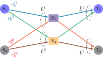
Figure 2: Network flow game with two players and two relay nodes.

In this section, we illustrate our results using a simplified version of the network-flow control game analyzed in [6]. The flow control problem involves two sources, denoted as $S_{1}$ and $S_{2}$, two destinations $T_{1}$ and $T_{2}$, and two relay nodes $N_{1}$ and $N_{2}$, as shown in Figure 2. Each player, represented by $i\in\{1,2\}$, can choose one of two possible paths ($S_{i}-N_{l}-T_{i}$, where $l\in\{1,2\}$) to transmit data from their respective source to the corresponding destination. We denote the flow along relay nodes $N_{1}$ and $N_{2}$ for player $i$ at time $k$ as $v_{k}^{i1}$ and $v_{k}^{i2}$, respectively. The relay nodes are equipped with batteries that deplete proportionally to the outgoing flow. The battery level evolution for relay node $l\in\{1,2\}$ is described by the following equation:

$$x_{k+1}^{l}=x_{k}^{l}-\delta^{l}(v_{k}^{1l}+v_{k}^{2l}),$$ (38)

where $\delta^{l}>0$ represents the proportional factor by which the battery level depletes due to data transmission through the relay node. Each user $i$ aims to maximize a rate-dependent concave utility function given by $\sum_{l=1}^{2}(w^{il}v_{k}^{il}-\tfrac{1}{2}t^{il}(v_{k}^{il})^{2})$, where $w^{il}$ and $t^{il}$ are positive constants, and $v_{k}^{il}$ represents the flow rate along path $l\in\{1,2\}$. Additionally, to conserve battery life, each player derives a payoff that depends on the battery level. This payoff is determined by the concave function $\sum_{l=1}^{2}(d^{il}x_{k}^{l}-\tfrac{1}{2}s^{il}(x_{k}^{l})^{2})$ during the decision time instants $k\in\mathsf{K}_{l}$, and by $\sum_{l=1}^{2}(D^{il}x_{K}^{l}-\tfrac{1}{2}S^{il}(x_{K}^{l})^{2})$ at time $K$. Consequently, each player $i\in\{1,2\}$ minimizes the cost function defined as:

$$J^{i}=-\beta^{K}\sum_{l=1}^{2}\big{(}D^{il}x_{K}^{l}-\tfrac{1}{2}S^{il}(x_{K}^{l})^{2}\big{)}\\ -\sum_{k=0}^{K-1}\sum_{l=1}^{2}\beta^{k}\Big{(}d^{il}x_{k}^{l}-\tfrac{1}{2}s^{il}(x_{k}^{l})^{2}+w^{il}v_{k}^{il}-\tfrac{1}{2}t^{il}(v_{k}^{il})^{2}\Big{)},$$ (39)

where $\beta\in(0,1)$ represents the discount factor. The constraints at each time instant $k\in\mathsf{K}_{l}$ are given by

$$\text{Relay: }L_{k}^{l}=v_{k}^{1l}+v_{k}^{2l}\leq c^{l}>0,~{}l=1,2,$$ (40a)

$$\text{Destination: }\tilde{L}_{k}^{i}=v_{k}^{i1}+v_{k}^{i2}\leq\tilde{c}^{i}>0,~{}i=1,2,$$ (40b)

$$\text{Battery: }x_{k+1}^{l}=x_{k}^{l}-\delta^{l}(v_{k}^{1l}+v_{k}^{2l})\geq{b^{l}_{min}},~{}l=1,2,$$ (40c)

$$\text{Transmission: }0\leq v_{k}^{il}\leq\bar{v}^{il}=\tfrac{w^{il}}{t^{il}},~{}i,l=1,2.$$ (40d)

Here, both coupled constraint (40a) and individual constraint (40b) indicate capacity constraints for both relay and destination nodes. Mixed constraint (40c) specifies that a relay node $l\in\{1,2\}$ cannot transmit data below its minimum battery level, ${b^{l}_{min}}\geq 0$. Additionally, constraint (40d) ensures that data transmitted from each source remains non-negative and is upper-bounded by $\frac{w^{il}}{t^{il}}$ (related to the concave increasing region of the rate-dependent payoff). Importantly, both players share relay nodes for data transmission. Due to capacity and battery level constraints, expressed respectively by (40a) and (40c), the transmission rates of the players are interdependent or coupled. With linear state dynamics (38), quadratic objectives (39), and inequality constraints (40), the network flow game fits into the DGC class. The network flow game is represented in standard form (1), with the state variable as $x_{k}=\mathrm{col}\{x_{k}^{1},x_{k}^{2},z_{k}\}$, where $z_{k}=1$ for $k\in\mathsf{K}$, and the decision variable for player $i$ on path $l$ as $u_{k}^{il}=v_{k}^{il}-\tfrac{w^{il}}{t^{il}}$ for $i=1,2$ and $l=1,2$. The parameters associated with this network flow game in standard form are given as follows

$$A_{k}=\begin{bmatrix}1&0&-\delta^{1}\alpha^{1}\\ 0&1&-\delta^{2}\alpha^{2}\\ 0&0&1\end{bmatrix},~{}B_{k}^{1}=B_{k}^{2}=\begin{bmatrix}-\delta^{1}&0\\ 0&-\delta^{2}\\ 0&0\end{bmatrix},$$

$$M^{i}_{k}=\mathrm{col}\{\mathbf{0}_{6\times 3},\tilde{M},\mathbf{0}_{1\times 3}\},~{}r_{k}^{i}=\mathrm{col}\{[r^{i}]_{l}\}_{l=1}^{9},~{}i=1,2,$$

$$[N^{1}_{k}]_{2}=[N^{2}_{k}]_{1}=\mathrm{col}\{\mathbf{0}_{4\times 2},\tilde{N}_{1},\tilde{N}_{2},\mathbf{0}_{1\times 2}\},$$

$$[N^{1}_{k}]_{1}=[N^{2}_{k}]_{2}=\mathrm{col}\{\mathbf{I}_{2\times 2},-\mathbf{I}_{2\times 2},\tilde{N}_{1},\tilde{N}_{2},[-1~{}-1]\},$$

$$\tilde{M}=\begin{bmatrix}1&0&0\\ 0&1&0\\ \end{bmatrix},~{}\tilde{N}_{1}=-\mathbf{I}_{2\times 2},~{}\tilde{N}_{2}=\begin{bmatrix}-\delta^{1}&0\\ 0&-\delta^{2}\end{bmatrix},$$

$$Q^{i}_{k}=\beta^{k}\begin{bmatrix}s^{i}&-d^{i}\\ -d^{i\prime}&-\alpha^{i+4}\end{bmatrix},~{}Q^{i}_{K}=\beta^{K}\begin{bmatrix}S^{i}&-D^{i}\\ -D^{i\prime}&0\end{bmatrix},$$

$$R_{k}^{ii}=\beta^{k}\oplus_{l=1}^{2}t^{il},~{}p_{k}^{i}=0,~{}R_{k}^{ij}=0,~{}i,j=1,2,~{}i\neq j,$$

$$\alpha^{1}=\tfrac{w^{11}}{t^{11}}+\tfrac{w^{21}}{t^{21}},~{}\alpha^{2}=\tfrac{w^{12}}{t^{12}}+\tfrac{w^{22}}{t^{22}},~{}\alpha^{3}=\tfrac{w^{11}}{t^{11}}+\tfrac{w^{12}}{t^{12}},$$

$$\alpha^{4}=\tfrac{w^{21}}{t^{21}}+\tfrac{w^{22}}{t^{22}},~{}\alpha^{5}=\tfrac{(w^{11})^{2}}{t^{11}}+\tfrac{(w^{12})^{2}}{t^{12}},~{}\alpha^{6}=\tfrac{(w^{21})^{2}}{t^{21}}+\tfrac{(w^{22})^{2}}{t^{22}},$$

$$[r^{i}]_{1}=\tfrac{w^{i1}}{t^{i1}},~{}[r^{i}]_{2}=\tfrac{w^{i2}}{t^{i2}},~{}[r^{i}]_{3}=[r^{i}]_{4}=0,~{}[r^{i}]_{5}=c^{1}-\alpha^{1},$$

$$[r^{i}]_{6}=c^{2}-\alpha^{2},~{}[r^{i}]_{7}=-\delta^{1}\alpha^{1}-b,[r^{i}]_{8}=-\delta^{2}\alpha^{2}-b,$$

$$[r^{1}]_{9}=\tilde{c}^{1}-\alpha^{3},~{}[r^{2}]_{9}=\tilde{c}^{2}-\alpha^{4},~{}S^{i}=\oplus_{l=1}^{2}S^{il},~{}s^{i}=\oplus_{l=1}^{2}s^{il},$$

$$d^{i}=\mathrm{col}\{d^{il}\}_{l=1}^{2},~{}D^{i}=\mathrm{col}\{D^{il}\}_{l=1}^{2},~{}i=1,2.$$

(a)

(b)

(c)

(d)

Figure 3: Flow-rates/controls of the players (panel (a)), battery levels (panel (b)), aggregate flow-rates at the relay nodes (panel (c)) and destination nodes (panel (d)). Arrow with equation number pointing to a dashed dark line indicates that one of the constraints (40) is active.

Remark 8.

By imposing the following constraints on the parameters: $s^{11}=s^{21}$, $s^{12}=s^{22}$, $S^{11}=S^{21}$, and $S^{21}=S^{22}$, we observe that the game parameters satisfy the sufficient conditions for an open-loop potential difference game, as outlined in [6, Lemma 3 and Lemma 4]. Nevertheless, these constraints restrict the range of strategic scenarios within the flow-control game. Consequently, the approach presented in [6] is unsuitable for computing a GOLNE in such cases.

The problem parameters are set as follows: $K=60,~{}x_{0}^{1}=9,~{}x_{0}^{2}=6,~{}b^{1}_{\min}=1,~{}b_{\min}^{2}=0.5,~{}\delta^{1}=0.125,~{}\delta^{2}=0.075,~{}\beta=0.95,~{}w^{11}=30,~{}w^{12}=16,~{}w^{21}=26,~{}w^{22}=10,~{}t^{i1}=t^{i2}=10,~{}d^{il}=6,~{}D^{il}=8.0,~{}s^{11}=6,~{}s^{12}=5.5,~{}s^{21}=7,~{}s^{22}=7.5,~{}S^{11}=8,~{}S^{12}=7.5,~{}S^{21}=9,~{}S^{22}=9.5,~{}{c}^{1}=5.4,~{}{c}^{2}=2.6,~{}\tilde{c}^{1}=4,~{}\tilde{c}^{2}=3$. We observe that these parameter values do not meet the sufficient conditions for an open-loop potential difference game, as indicated in Remark 8. Therefore, the optimization-based approach employed in [6] is not applicable for computing GOLNE. It is easily verified that the conditions required in Theorems 6 are satisfied for the chosen parameter values. We used the freely available PATH solver (available at https://pages.cs.wisc.edu/ferris/path.html) for solving the LCP (37). The flow-rate constraints (40), with the above parameter values are given by

Transmission: $$0\leq v_{k}^{11}\leq 3,~{}0\leq v_{k}^{12}\leq 1.6$$

$$0\leq v_{k}^{21}\leq 2.6,~{}0\leq v_{k}^{22}\leq 1$$

Relay: $$v_{k}^{11}+v_{k}^{21}\leq 5.4,~{}v^{12}_{k}+v_{k}^{22}\leq 2.6$$

Destination: $$v_{k}^{11}+v_{k}^{12}\leq 4,~{}v_{k}^{21}+v_{k}^{22}\leq 3$$

Battery: $$x_{k}^{1}-0.125(v_{k}^{11}+v_{k}^{21})\geq 1$$

$$x_{k}^{2}-0.075(v_{k}^{12}+v_{k}^{22})\geq 0.5.$$

We note that the transmission rate-dependent utility is concave, indicating that players receive higher payoffs by increasing their flow rates. However, they are also incentivized to reduce their flow rates due to the concave, increasing battery-level-dependent payoff. Fig. 3 illustrates a comparison of individual and aggregate flow rates, as well as the relay battery levels, with GOLNE strategies. Initially, both players reduce their flows through relay node $N_{1}$, which depletes faster than relay node $N_{2}$; see Fig. 3a. They then increase their flows through relay node $N_{2}$. At relay node $N_{2}$, players transmit at their peak individual rates, i.e., $v_{k}^{12}=1.6$ and $v_{k}^{22}=1$, which also meet the maximum capacity of the relay node; see Fig. 3a and 3c. Since players cannot transmit any further through node $N_{2}$, they maintain a constant rate through node $N_{1}$, which has a larger capacity. These constant levels are determined by the capacity constraints at the destination nodes, specifically $\tilde{c}^{1}=v_{k}^{11}+v_{k}^{12}\rightarrow v_{k}^{11}=4-1.6=2.4$ and $\tilde{c}^{2}=v_{k}^{21}+v_{k}^{22}\rightarrow v_{k}^{21}=3-1=2$; see Fig. 3a and 3d. We observe that the aggregate flow rates through node $N_{1}$ are not saturated at maximum capacity because players self-limit their flows to conserve battery life. On the other hand, at relay node $N_{2}$, the capacity constraint is more restrictive than the self-limitation incentive towards conserving battery life. Consequently, the players’ GOLNE flow rates reflect a trade-off between these conflicting objectives. The players stop transmitting once the battery levels at the relay nodes reach the minimum levels, that is, relay node $N_{1}$ at $t=25$ and relay node $N_{2}$ at $t=48$; see Fig. 3b.

5 Conclusions

We studied a class of linear quadratic difference games with coupled-affine inequality constraints. We derived both the necessary and sufficient conditions for the existence of a generalized open-loop Nash equilibrium by establishing an equivalence between solutions of specific discrete-time linear complementarity systems and the convexity of players’ objective functions. With additional assumptions, we demonstrated that GOLNE strategies can be obtained by solving a large-scale linear complementarity problem. As part of our future work, we plan to investigate the existence of a generalized feedback Nash equilibrium within this class of dynamic games.

Notations for Section 3.3

We define $\mathbf{R}_{k}=\oplus_{i=1}^{N}R_{k}^{ii}$, $\mathbf{B}_{k}=\oplus_{i=1}^{N}B_{k}^{i}$, $\mathbf{N}_{k}=\oplus_{i=1}^{N}[N^{i}_{k}]_{i}$, $\mathbf{M}_{k}=\oplus_{i=1}^{N}M^{i}_{k}$, $\mathbf{r}_{k}=\mathrm{col}\{r_{k}^{i}\}_{i=1}^{N}$, $\mathsf{u}_{k}^{\star}=\mathrm{col}\{u_{k}^{i\star}\}_{i=1}^{N}$, $\bm{\upmu}_{k}^{\star}=\mathrm{col}\{\mu_{k}^{i\star}\}_{i=1}^{N}$,  $k\in\mathsf{K}_{l}$, $\mathbf{p}_{k}=\mathrm{col}\{p_{k}^{i}\}_{i=1}^{N}$, $P_{k}=\mathrm{col}\{P_{k}^{i}\}_{i=1}^{N}$, $\bm{\zeta}_{k}=\mathrm{col}\{\zeta_{k}^{i}\}_{i=1}^{N}$, $k\in\mathsf{K}$.   In (33): $\mathbf{G}_{k}=(\Lambda_{k})^{-1}A_{k}$, $[\overline{\mathbf{G}}_{k+1}]_{i}=-(\Lambda_{k})^{-1}B^{i}_{k}(R^{ii}_{k})^{-1}{B^{i}_{k}}^{\prime}$, $[\tilde{\mathbf{G}}_{k}]_{i}=(\Lambda_{k})^{-1}B^{i}_{k}(R^{ii}_{k})^{-1}[N^{i}_{k}]_{i}^{\prime}$, $\mathbf{F}_{k}=-(\mathbf{R}_{k})^{-1}\mathbf{B}_{k}^{\prime}P_{k+1}\mathbf{G}_{k}$, $\overline{\mathbf{F}}_{k+1}=-(\mathbf{R}_{k})^{-1}\mathbf{B}_{k}^{\prime}(\mathbf{I}+P_{k+1}\overline{\mathbf{G}}_{k+1})$, $\tilde{\mathbf{F}}_{k}=(\mathbf{R}_{k})^{-1}(\mathbf{N}_{k}^{\prime}-\mathbf{B}_{k}^{\prime}P_{k+1}\tilde{\mathbf{G}}_{k})$, $\mathbf{H}_{k+1}=(\mathbf{I}_{N}\otimes A_{k}^{\prime})(\mathbf{I}+P_{k+1}\overline{\mathbf{G}}_{k+1})$, $\overline{\mathbf{H}}_{k}=(\mathbf{I}_{N}\otimes A_{k}^{\prime})P_{k+1}\tilde{\mathbf{G}}_{k}-\mathbf{M}_{k}^{\prime}$ for $k\in\mathsf{K}_{l}$.  For the state transition matrices in (33a)-(33b): $\phi(k,\tau)=\mathbf{G}_{k-1}\mathbf{G}_{k-2}\cdots\mathbf{G}_{\tau}$ for $k>\tau$ and $\phi(k,\tau)=\mathbf{I}$ for $k=\tau$, $k,\tau\in\mathsf{K}$. $\varphi(k,\tau)=\mathbf{H}_{k+1}\mathbf{H}_{k+2}\cdots\mathbf{H}_{\tau}$ for $k<\tau$ and $\varphi(k,\tau)=\mathbf{I}$ for $k=\tau$, $k,\tau\in\mathsf{K}_{l}$.  In (35): $x_{\mathsf{K}}^{\star}=\mathrm{col}\{x_{k}^{\star}\}_{k=0}^{K-1}$, $\mathsf{u}^{\star}_{\mathsf{K}}=\mathrm{col}\{\mathsf{u}^{\star}_{k}\}_{k=0}^{K-1}$, $\bm{\upmu}^{\star}_{\mathsf{K}}=\mathrm{col}\{\bm{\upmu}^{\star}_{k}\}_{k=0}^{K-1}$, $\mathbf{p}_{\mathsf{K}}=\mathrm{col}\{\mathbf{p}_{k+1}\}_{k=0}^{K-1}$, $\bm{\zeta}_{\mathsf{K}}=\mathrm{col}\{\bm{\zeta}_{k+1}\}_{k=0}^{K-1}$, $\textbf{r}_{\mathsf{K}}=\mathrm{col}\{\textbf{r}_{k}\}_{k=0}^{K-1}$, $\mathbf{F}_{\mathsf{K}}=\oplus_{k=0}^{K-1}\mathbf{F}_{k}$, $\overline{\mathbf{F}}_{\mathsf{K}}=\oplus_{k=0}^{K-1}\overline{\mathbf{F}}_{k+1}$, $\tilde{\mathbf{F}}_{\mathsf{K}}=\oplus_{k=0}^{K-1}\tilde{\mathbf{F}}_{k}$, $[\bm{\Phi}_{0}]_{k}=\phi(k-1,0)$, $[\bm{\Phi}_{1}]_{1\tau}=\mathbf{0}$, $[\bm{\Phi}_{2}]_{1\tau}=\mathbf{0}$, $[\bm{\Phi}_{1}]_{k\tau}=\sum_{\rho=1}^{\mathrm{min}\,\,(k-1,\tau-1)}\phi(k-1,\rho)\overline{\mathbf{G}}_{\rho}\varphi(\rho,\tau-1)$ for $k>1$, $[\bm{\Phi}_{2}]_{k\tau}=\phi(k-1,1)\tilde{\mathbf{G}}_{0}$ for $k>\tau=1$, $[\bm{\Phi}_{2}]_{k\tau}=\big{(}\sum_{\rho=1}^{\tau-1}\phi(k-1,\rho)\overline{\mathbf{G}}_{\rho}\varphi(\rho,\tau-1)\big{)}\overline{\mathbf{H}}_{\tau-1}+\phi(k-1,\tau)\tilde{\mathbf{G}}_{\tau-1}$ for $1<\tau<k$, $[\bm{\Phi}_{2}]_{k\tau}=\big{(}\sum_{\rho=1}^{k-1}\phi(k-1,\rho)\overline{\mathbf{G}}_{\rho}\varphi(\rho,\tau-1)\big{)}\overline{\mathbf{H}}_{\tau-1}$ for $\tau\geq k$ $[\bm{\Psi}_{1}]_{k\tau}=\varphi(k,\tau)$, $[\bm{\Psi}_{2}]_{k\tau}=\varphi(k,\tau-1)\overline{\mathbf{H}}_{\tau-1}$ for $\tau\geq k$, $[\bm{\Psi}_{1}]_{k\tau}=\mathbf{0}$, $[\bm{\Psi}_{2}]_{k\tau}=\mathbf{0}$ for $\tau<k$ with $k,\tau\in\mathsf{K}_{r}$, $\mathsf{M}_{\mathsf{K}}=\oplus_{k=0}^{K-1}(\overline{\mathbf{M}}_{k}+\overline{\mathbf{N}}_{k}\mathbf{F}_{k})$, $\mathsf{N}_{\mathsf{K}}=\oplus_{k=0}^{K-1}(\overline{\mathbf{N}}_{k}\overline{\mathbf{F}}_{k+1})$ and $\tilde{\mathsf{N}}_{\mathsf{K}}=\oplus_{k=0}^{K-1}(\overline{\mathbf{N}}_{k}\tilde{\mathbf{F}}_{k})$.

References

- [1] R. Isaacs, Differential Games. John Wiley and Sons, 1965.
- [2] J. Engwerda, LQ dynamic optimization and differential games. John Wiley & Sons, 2005.
- [3] T. Başar and G. Olsder, Dynamic Noncooperative Game Theory, ser. Classics in Applied Mathematics. SIAM, 1999.
- [4] E. Dockner, S. Jorgensen, N. Van Long, and G. Sorger, Differential Games in Economics and Management Science. Cambridge University Press, 2000.
- [5] Q. Zhu and T. Basar, “Game-theoretic methods for robustness, security, and resilience of cyberphysical control systems: games-in-games principle for optimal cross-layer resilient control systems,” IEEE Control Systems Magazine, vol. 35, no. 1, pp. 46–65, 2015.
- [6] S. Zazo, S. V. Macua, M. Sánchez-Fernández, and J. Zazo, “Dynamic potential games with constraints: Fundamentals and applications in communications,” IEEE Transactions on Signal Processing, vol. 64, no. 14, pp. 3806–3821, 2016.
- [7] J. Chen and Q. Zhu, “A game-theoretic framework for resilient and distributed generation control of renewable energies in microgrids,” IEEE Transactions on Smart Grid, vol. 8, no. 1, pp. 285–295, 2016.
- [8] K. J. Arrow and G. Debreu, “Existence of an equilibrium for a competitive economy,” Econometrica, vol. 22, no. 3, pp. 265–290, 1954.
- [9] J. B. Rosen, “Existence and uniqueness of equilibrium points for concave n-person games,” Econometrica, pp. 520–534, 1965.
- [10] P. T. Harker, “Generalized Nash games and quasi-variational inequalities,” European journal of Operational research, vol. 54, no. 1, pp. 81–94, 1991.
- [11] F. Facchinei and C. Kanzow, “Generalized Nash equilibrium problems,” 4OR, vol. 5, no. 3, pp. 173–210, Sep 2007.
- [12] G. Belgioioso, P. Yi, S. Grammatico, and L. Pavel, “Distributed generalized Nash equilibrium seeking: An operator-theoretic perspective,” IEEE Control Systems Magazine, vol. 42, no. 4, pp. 87–102, 2022.
- [13] J. C. Engwerda and Salmah, “The open-loop linear quadratic differential game for index one descriptor systems,” Automatica, vol. 45, no. 2, pp. 585–592, 2009.
- [14] ——, “Feedback Nash equilibria for linear quadratic descriptor differential games,” Automatica, vol. 48, no. 4, pp. 625–631, 2012.
- [15] P. V. Reddy and J. C. Engwerda, “Feedback properties of descriptor systems using matrix projectors and applications to descriptor differential games,” SIAM Journal on Matrix Analysis and Applications, vol. 34, no. 2, pp. 686–708, 2013.
- [16] A. Tanwani and Q. Zhu, “Feedback Nash equilibrium for randomly switching differential–algebraic games,” IEEE Transactions on Automatic Control, vol. 65, no. 8, pp. 3286–3301, 2020.
- [17] R. Singh and A. Wiszniewska-Matyszkiel, “Discontinuous Nash equilibria in a two-stage linear-quadratic dynamic game with linear constraints,” IEEE Transactions on Automatic Control, vol. 64, no. 7, pp. 3074–3079, 2019.
- [18] F. Laine, D. Fridovich-Keil, C.-Y. Chiu, and C. Tomlin, “The computation of approximate generalized feedback Nash equilibria,” SIAM Journal on Optimization, vol. 33, no. 1, pp. 294–318, 2023.
- [19] P. V. Reddy and G. Zaccour, “Open-Loop Nash Equilibria in a Class of Linear-Quadratic Difference Games With Constraints,” IEEE Transactions on Automatic Control, vol. 60, no. 9, pp. 2559–2564, 2015.
- [20] ——, “Feedback Nash Equilibria in Linear-Quadratic Difference Games With Constraints,” IEEE Transactions on Automatic Control, vol. 62, no. 2, pp. 590–604, 2017.
- [21] P. S. Mohapatra and P. V. Reddy, “Linear-quadratic mean-field-type difference games with coupled-affine inequality constraints,” IEEE Control Systems Letters, vol. 7, pp. 1987–1992, 2023.
- [22] G. Jank and H. Abou-Kandil, “Existence and uniqueness of open-loop Nash equilibria in linear-quadratic discrete time games,” IEEE Transactions on Automatic Control, vol. 48, no. 2, pp. 267–271, 2003.
- [23] S. Sethi and G. Thompson, Optimal Control Theory: Applications to Management Science and Economics. Springer, 2006.
- [24] W. P. M. H. Heemels, J. M. Schumacher, and S. Weiland, “Linear complementarity systems,” SIAM Journal on Applied Mathematics, vol. 60, no. 4, pp. 1234–1269, 2000.
- [25] A. J. van der Schaft and H. Schumacher, An Introduction to Hybrid Dynamical Systems, ser. Lecture Notes in Control and Information Sciences. Springer London, 2007.
- [26] R. W. Cottle, J.-S. Pang, and R. E. Stone, The linear complementarity problem, ser. Classics in Applied Mathematics. SIAM, 2009.