Abstract

Heavy particles in vortical fluid flow cluster strongly, forming singular structures termed caustics for their resemblance to focal surfaces in optics. We show here that such extreme aggregation onto low-dimensional submanifolds can arise without inertia for self-propelled particles (SPPs). We establish that a singular perturbation is at the heart of caustic formation by SPPs around a single vortex, and our numerical studies of SPPs in two-dimensional Navier-Stokes turbulence shows intense caustics in the straining regions of the flow, peaking at intermediate levels of self-propulsion. Our work offers a route to singularly high local concentrations in a macroscopically dilute suspension of zero-Reynolds number swimmers, with potentially game-changing implications for communication and sexual reproduction. An intriguing open direction is whether the active turbulence of a suspension of swimming microbes could serve to generate caustics in its own concentration.

Introduction

The motion of particles in an ambient flow governs the formation of droplets in clouds PINSKY19971177 , the drift of atmospheric pollutants Fernando2010 and the biological pump of the oceans Boyd , and is central to a wide range of industrial processes SAMBORSKA2022110960 . When the particles have appreciable inertia, the coupling between their velocity and the local flow profile can lead to long-wavelength inhomogeneities in their spatial distribution Lillo2004 . Heavy particles in a background turbulent flow are known to get centrifuged out of regions of high vorticity. Vortices thus promote particle collisions, aggregation, and caustics MR1983 ; Maxey1986 ; Croor2015 ; Wilkinson_2005 , offering a plausible mechanism for droplet growth in clouds Croor2017 . In this article we explore theoretically the possibility that such singular enhancement of encounters might occur in suspensions of motile particles lauga2009hydrodynamics without particle inertia, dramatically increasing opportunities for communication and sexual reproduction BUSKEY199813 among small, slow, persistent swimmers in marine environments Tuval2020 ; StockerARFM2012 .

Biological motility in a fluid medium Tuval2020 is dynamic, and flows can strongly influence the dispersal of swimmers PhysRevLett.129.064502 ; PhysRevFluids.6.L012501 yielding features such as preferential sampling in turbulence Durham2013 ; PhysRevLett.116.108104 . The competition between autonomous motion and systematic reorientation by the mean ambient flow field $\mathbf{U}$ is characterised by the ratio $\beta/\mathinner{\!\left\lVert\nabla\mathbf{U}\right\rVert}$ where $1/\beta$ is the time it takes for a swimmer to move by its own body length. Our focus in this work is on swimmers with vanishingly small Stokes and Reynolds numbers, with self-propelling stresses small compared to those created by the ambient flow. We therefore ignore particle inertia as well as the effect of the particles on the flow. Microscopic marine plankton, in particular, operate in this regime, in a vortex-laden turbulent ecosystem, and the coupling of their motility with ambient flow Denny1997 ; Tuval2020 ; StockerARFM2012 ; Krishnamurthy2020 ; mousavi2023efficient ; Durham2013 plays a central role in their lives. Fig. 1 (a) depicts typical values of $\beta/\mathinner{\!\left\lVert\nabla\mathbf{U}\right\rVert}$ and $Re$ for various swimmers, based on published data on swimming speed and size, and typical shear-rates in the upper mixed layer of the open ocean StockerARFM2012 [see Supplementary].

Micro-swimmers in externally driven flows, through the coupling of their orientation to velocity gradients pedley1992hydrodynamic ; Torney2007 ; Zhan2014 , display focusing Kessler1985 , aggregation GENIN20043 ; Ardekani2012 , and expulsion out of vortical regions Sokolov2016 , in a manner reminiscent of inertial particles Croor2015 ; Wilkinson_2005 . Although their inertia is negligible, their motion is persistent because of self-propulsion Durham2013 . Moreover, the Hamiltonian structure of bound orbits of microswimmers in certain flows Stark2016 ; Lushi2015 ; Shelley2019 ; Arguedas_Leiva_2020 suggests a role for the effective inertial dynamics of active Stokesian suspensions in imposed flows, where the orientation vector behaves like momentum Chajwa2019 ; Ronojoy2020 ; Chajwa2020 .

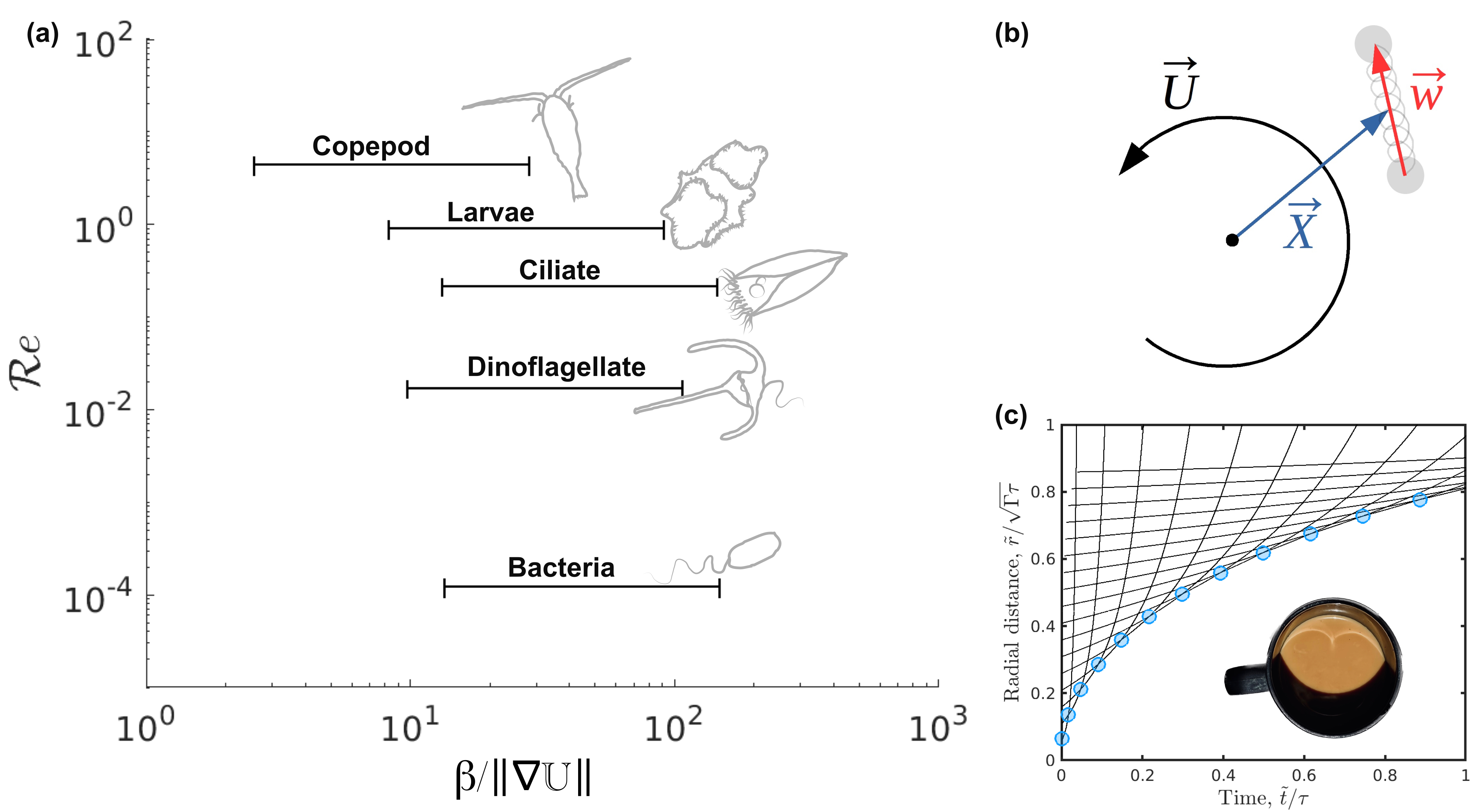
Figure 1: Active dimer model for self-propelled particles in ambient flow (a) We depict typical values of the ratio of flow time scale $1/\mathinner{\!\left\lVert\nabla\mathbf{U}\right\rVert}$ to swimming time scale $1/\beta$, and Reynolds number $Re$ for a marine bacterium Vibrio alginolyticus doi:10.1073/pnas.1602307113 , various dinoflagellates, ciliates Lauga2019 , invertebrate larvae FUCHS2016109 and copepods FUCHS2016109 . For $\mathinner{\!\left\lVert\nabla\mathbf{U}\right\rVert}$ we substitute the Kolmogorov shear rate for the range of previously measured energy dissipation rates in the upper mixed layer of the ocean $10^{-8}-10^{-6}$ m²s^-3 StockerARFM2012 (see Supplementary). (b) Schematic of an active dimer of extension $\mathbf{w}$ in a flow $\mathbf{U}$. (c) Caustics based on the inner solution are marked by the intersection of representative trajectories (blue circles) of particles starting at closely separated initial radial distances, with $\alpha=0.1$. A continuous variation in $\tilde{r}_{0}$ would give a continuous curve. The inset (Photo credit: R. Chajwa) is an image of optical caustics with a similar cusp on the surface of coffee in a mug.

We ask if inertia-less swimmers pedley1992hydrodynamic can display caustics, a conspicuous encounter-promoting feature of the dynamics of inertial particles (IPs) in flows, where the calculated worldlines of suspended particles cross, so the solute velocity field is multivalued Wilkinson_2005 ; Croor2015 . We investigate this intriguing possibility theoretically, in the simple setting of a dilute suspension of neutrally buoyant swimmers in two-dimensional vortical flows. We find that non-inertial active particles, like passive but inertial particles, can display caustics even near a single vortex, a building block of turbulence. We show how far the analogy with IP may be carried, and where the two differ fundamentally. Our flow geometry allows unambiguous demarcation of the regimes of caustic formation, and forms the basis for understanding the behavior of active particles in unsteady vortical flows like turbulence. We examine the flow-coupled dynamics of two simple models of single motile particles: Hookean and preferred-length active dimers, corresponding, in the presence of noise, to active Ornstein-Uhlenbeck particles (AOUPs) Howfar2016 and active Brownian particles (ABPs) Romanczuk2012 respectively.

Results

Connecting active and inertial dynamics

The motion of an IP with position vector $\mathbf{X}$ in a background flow-field $\mathbf{U}$ is governed by the Maxey-Riley MR1983 equation which, to leading order in gradients, reads $\dot{\mathbf{X}}=\mathbf{v}$ and $\text{St}\,\dot{\mathbf{v}}=\,(\mathbf{U}-\mathbf{v})$, when non-dimensionalised using a characteristic particle length scale $d$ and a flow velocity scale $U_{0}$. The Stokes number $\text{St}=\tau U_{0}/d$ is a non-dimensional measure of inertia, characterised by the relaxation time $\tau$ ($=$ mass/Stokes drag coefficient) of a particle. The centrifugation of these particles away from the vortex centre results in the formation of caustics within a critical distance from the vortex origin Croor2015 . Setting $\text{St}=0$ yields tracer particles, which move with $\mathbf{v}=\mathbf{U}$.

To demonstrate analytically that caustics and the consequent discontinuities in particle number densities can arise due to activity, even without inertia, we consider a Hookean active dimer, with centroid position $\mathbf{X}$ and end-to-end vector $\mathbf{w}$, placed in an imposed background flow field $\mathbf{U}$. We work at zero Stokes number and thus neglect particle inertia, but, as we see below, self-propulsion allows the particle to cross streamlines. In the absence of translational diffusion the equations of motion for $\mathbf{X}$ and $\mathbf{w}$ then take the first-order form

$$\dot{\mathbf{X}}=\mu\mathbf{F}\,+\mathbf{U}\,+\beta\mathbf{w}\,\equiv\,\mathbf{v},$$ (1a)

$$\dot{\mathbf{w}}=-\frac{\mathbf{w}}{\tau}\,+\,(\alpha\,\textsf{{S}}+\textsf{{A}}\,)\cdot\,\mathbf{w}-\ell^{2}\nabla^{2}\mathbf{U}\,+\sqrt{2D}\bm{\eta},$$ (1b)

where $\mu$ is the Stokesian mobility of the particle, and $\mathbf{U}$, $\nabla^{2}\mathbf{U}$ and the external force field $\mathbf{F}$ are evaluated at $\mathbf{X}(t)$. In (1b) $\beta$, with units of inverse time but indefinite sign, endows a dimer with self-propulsion proportional to its extension, and the polar flow-alignment parameter $\ell$, with units of length, orients the dimer along a locally parabolic flow, and vanishes for an apolar, i.e., fore-aft symmetric, particle. For a review of microswimmers in imposed flow-fields, though without the polar coupling $\ell$, see Stark2016 . The analog of $\ell$ for a collective orientation vector appears in maitra2014activating . Apolar flow-orientation couplings Jeffery1922 enter through the strain-rate and vorticity tensors $\textsf{{S}}\equiv(\nabla\mathbf{U}+\nabla\mathbf{U}^{\top})/2$ and $\textsf{{A}}\equiv(\nabla\mathbf{U}-\nabla\mathbf{U}^{\top})/2$ respectively, with a response parameter $\alpha$ determined by particle shape. In (1b) $\bm{\eta}$ is a zero-mean, isotropic, gaussian white noise with unit variance.

For $\beta\neq 0$, (1a) and (1b) yield an equation for the total active-particle velocity ${\bf v}$ [see (1a)] viewed as a dynamical variable, displayed here for constant spatially uniform external force ${\bf F}$, and in general form in the Supplement:

$$\frac{\tau}{\mu}\dot{\mathbf{v}}=\left[-\frac{1}{\mu}\textsf{{I}}+\frac{\tau}{\mu}(\alpha+1)\textsf{{S}}\right]({\bf v}-{\bf U})+{\bf F}+\frac{\tau}{\mu}(D_{t}-\beta\ell^{2}\nabla^{2}){\bf U}+\frac{\tau\beta}{\mu}\sqrt{2D}\bm{\eta}$$ (2)

where $D_{t}=\partial_{t}+{\bf U}\cdot\nabla$, and all fields are evaluated at $\mathbf{X}(t)$. In the absence of $\ell^{2}\nabla^{2}\mathbf{U}$ and $\bm{\eta}$ (1b) is homogeneous, so that $\beta$ can be absorbed into $\mathbf{w}$ in (1). This is why $\beta$ appears only as a prefactor of $\nabla^{2}\mathbf{U}$ and $\bm{\eta}$ in (2). However, (1) can be recast as (2) only if $\mathbf{w}$, i.e., self-propulsion, enters (1a); the degree to which it does is governed by $\tau$. For $\tau\to 0$, (1b) implies $\mathbf{w}=0$.

The presence in (2) of the external force and the drag, unmodified by prefactors, means that $\tau/\mu$ plays the role of an effective mass for this inertia-less active system. Indeed (2) resembles the Maxey-Riley equation for inertial particles in a flow MR1983 . There are differences, such as the absence in (2) of the Basset-Boussinesq history term MR1983 ; prasath2019accurate , but the intriguing similarities prompt us to explore analogs to passive inertial-particle behavior in the dynamics of active inertia-less particles in external flows.

Caustics near a point vortex flow

We begin with the classical case of motion in the flow field of a point vortex at the origin. In plane polar coordinates $(r,\theta)$, $\mathbf{U}=\hat{\theta}\tilde{\Gamma}/r$, with circulation $2\pi\tilde{\Gamma}$. Note that $\textsf{{A}}=0$ for this flow everywhere except at the origin. Non-dimensionalizing (2) using the natural length $\sqrt{\tilde{\Gamma}\tau}$ Croor2015 and time $\tau$ gives the coupled equations

$$\ddot{r}-\frac{L^{2}}{r^{3}}=-\dot{r}+\frac{\alpha}{r^{3}}-\frac{(1+\alpha)L}{r^{3}},$$ (3a)

$$\dot{L}=1-L-\frac{(1+\alpha)\dot{r}}{r}+\frac{\lambda}{r^{2}},$$ (3b)

(see Supplementary) for the Lagrangian dynamics of the active particle whose centroid is at a radial distance of $r$ from a point vortex, where $L\equiv r^{2}\dot{\theta}$ is the angular momentum per unit mass of the particle and $\lambda\equiv\beta\ell^{2}/\tilde{\Gamma}$.

Effective centrifugal accelerations, reinforcing the similarity to an IP, arise through the $L^{2}/r^{3}$ term. Due to the terms containing $\alpha$, our equations are distinct from those for true IP Croor2015 . In this part of our analysis we limit ourselves to particles with apolar, i.e., fore-aft symmetric, shape, so that $\lambda=0$. We treat the nonlinearities in (3a) & (3b) perturbatively. A regular perturbation approach yields absurd solutions near the origin; in fact equations (3a) and (3b) constitute a singular perturbation problem BO1999 . The behaviour at very small times and small distances away from the vortex is singular, and relatively violent, unlike the more gentle relaxation to the final state at late times. We exploit this feature to understand the different physics at small and large time.

We seek an inner solution at the lowest order for $t\ll 1$ and $r\ll 1$, and an outer solution for $t\gg 1$, where $r$ could be $O(1)$ or larger. In contrast to an IP which centrifuges out forever, the outer solution for an active Hookean dimer is steady rotation with $\mathbf{w}$ and $\dot{\theta}=1/r_{f}^{2}$ at a constant final distance $r_{f}$ from the vortex, rendering the particle passive and lifeless at large times. Intriguing physics appears in the inner region, which sets the stage for the rest of this article. As is standard in singular perturbation theory, we recast (3a) and (3b) in the stretched spatial $\tilde{r}\equiv r/\delta_{i}$ and temporal $\tilde{t}\equiv t/\epsilon_{i}$ variables, where $\epsilon_{i}$ and $\delta_{i}$ are as yet unknown, but will be selected to ensure that all derivatives in the stretched variables are $\mathcal{O}(1)$. Dominant balance necessitates $\epsilon_{i}=\delta_{i}^{2}$, yielding the inner solution $L(\tilde{r})=L_{0}-(1+\alpha)\log{\tilde{r}/\tilde{r}_{0}}$, and the dynamics $\dot{\tilde{r}}=\partial\mathcal{H}/\partial p$ and $\dot{p}=-\partial\mathcal{H}/\partial\tilde{r}$ with an effective Hamiltonian

$$\mathcal{H}=\frac{p^{2}}{2}+\frac{\alpha+[L(\tilde{r})-1-\alpha]^{2}}{2\tilde{r}^{2}}$$ (4)

where $p\equiv d\tilde{r}/d\tilde{t}$ is the radial momentum per unit mass of the particle, and the subscript $0$ indicates an initial value.

Each solution is a ray in the $(t,r)$ plane, and some representative rays are shown in Fig. 1. We start out with two rings of particles around the vortex at initial radii $r_{0}$ and $r_{0}+\Delta r$. The intersection of their rays in the $r,t$ plane represents an overtaking of the outer ring by the inner, i.e., the occurrence of caustics. Caustics for a few chosen $r_{0}$ are shown by the blue circles in Fig.1(c), along with the envelope (continuous line) for all $r_{0}$, representing the smallest radial distance at a given time for the occurrence of caustics. For the purpose of demonstration we have taken $L_{0}=-(1+\alpha)\log\tilde{r}_{0}$, and equal initial speeds. This picture is akin to geometrical optics, where a caustic is an envelope tangent to the light rays eggers_fontelos_2015 .

In an alternative approach to demarcating caustics, which yields the same answers, we assume a continuum of particles described by its velocity field $\mathbf{v}(x,t)$. Caustics occur when $\mathbf{\nabla}\cdot\mathbf{v}\to-\infty$ meibohm2d2021 . We can define a particle velocity gradient Z whose evolution equation can be obtained directly from (2) (see equation 36 Supplementary Material). This equation may be solved in the Lagrangian frame of an individual particle, and caustics form where $\operatorname{Tr}{\textsf{{Z}}}\to-\infty$ meibohm2d2021 .

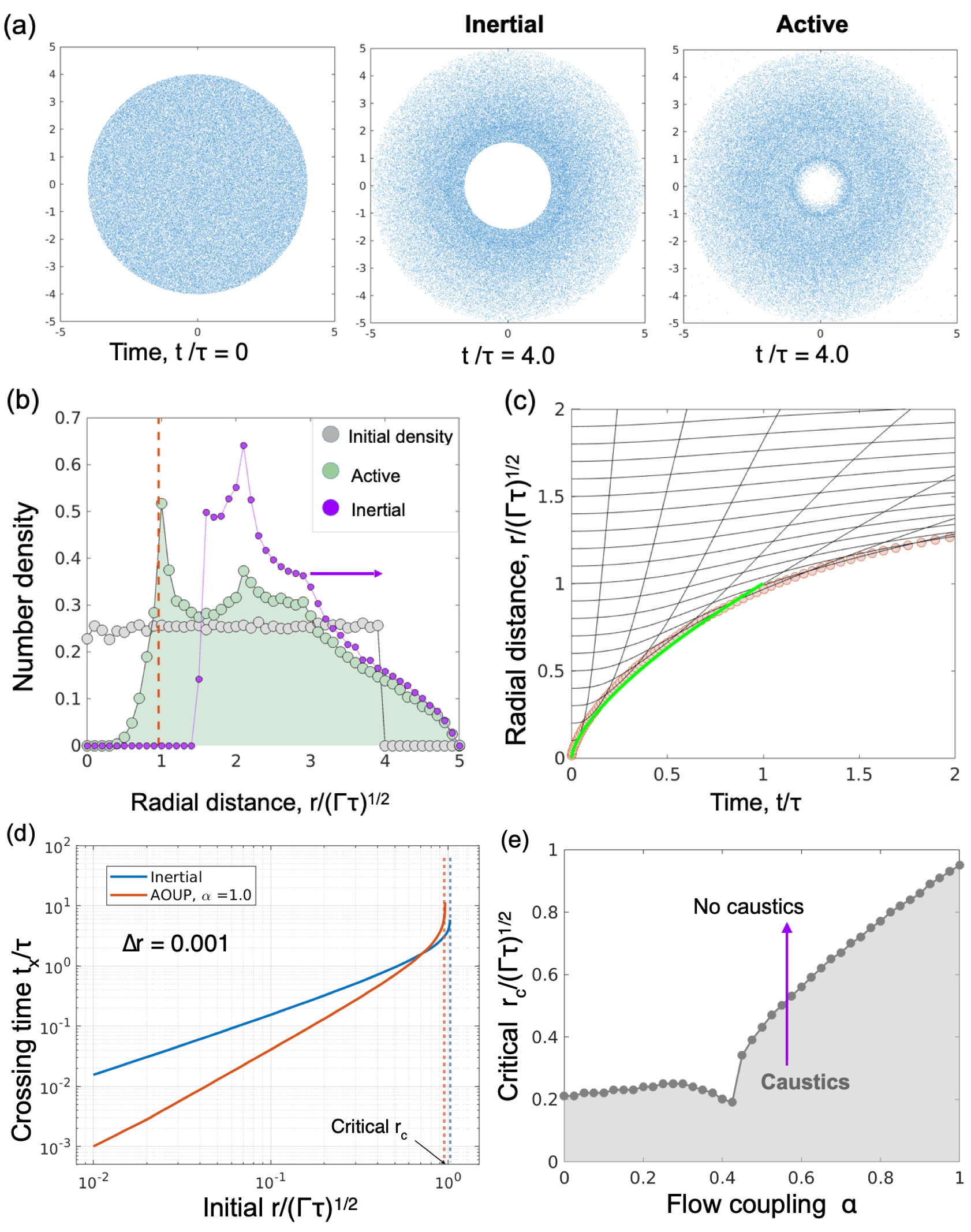
Figure 2: Centrifugation and caustics of dimer in point vortex: (a) Time frames showing the positions of the particles (blue dots) around a point vortex at the origin for IP and noiseless AOUP respectively [see Supplementary video 3.1 & 3.2]. Particles were initialised with uniformly random initial positions and orientations/velocities. (b) An initially homogeneous number-density (grey circles) peaks near a critical radial distance (green) in the steady state, compared to unsteady density of IP (purple) at a representative $t\gg 1$. (c) Trajectory (rays) of particles averaged over all initial orientations. The envelope of rays, for particles starting at various initial $r$, gives rise to caustics (red circles). The green curve shows $R=t^{\nu}$, with $\nu=2/3$. In (b), (c) & (d), $\alpha=1$. (d) The crossing time of adjacent rays separated by $\Delta r=0.001$ starting at various radial distances $r$, averaged over uniformly random initial orientations, diverges at a finite critical radius $r_{c}$ for an active particle (red) and for an inertial particle (blue) averaged over uniformly random initial velocity of unit magnitude. (e) For various $\alpha$, plotting $r_{c}$ demarcates the region of caustics, which is the radial distance below which adjacent rays cross each other in a finite time.

We now numerically solve the full equations (1a) and (1b), with the noise, the external force ${\bf F}$, and the polar flow coupling $\lambda$ set to zero (see Supplementary Video 1). In this case the self-propulsion $\beta$ can be absorbed in the definition of $\mathbf{w}$.

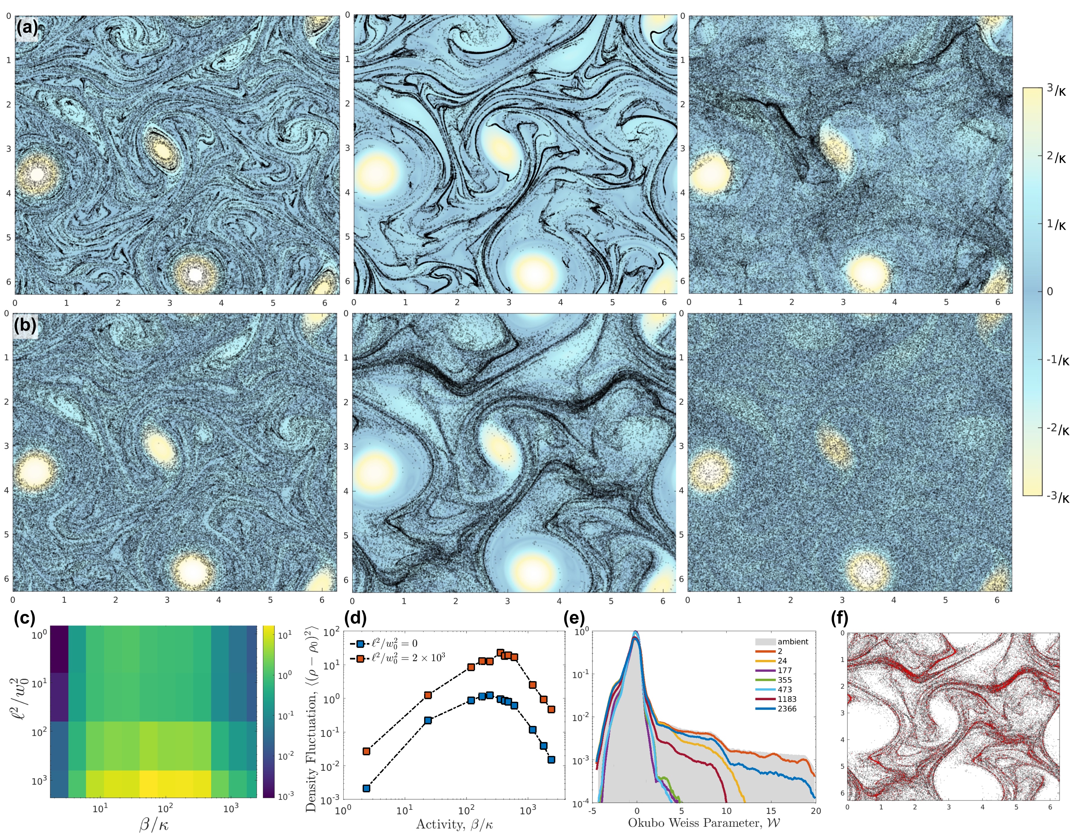
Figure 3: Caustics in turbulent flow. The blue-yellow colorbar represents the vorticity magnitude in the ambient turbulent flow scaled by the root-mean-square velocity gradient $\kappa=0.8454$s^-1 and black speckles are the locations of the geometric centers of $10^{5}$ active dimers with preferred length $w_{0}=500\mu m$. (a) $\ell^{2}/w_{0}^{2}=2\times 10^{3}$ with (from left to right) $\beta/\kappa=23.6$, $236$, and $2360$. (b) $\ell^{2}/w_{0}^{2}=0$ with (left to right) $\beta/\kappa=23.6$, $236$, and $2360$. For intermediate activity the particles display pronounced caustics [see Supplementary video].(c) heat-map of the number-density fluctuation plotted in $(\beta/\kappa,\ell^{2}/w_{0}^{2})$ plane. For comparison with plankton motility see Fig. 1 (a). (d) number-density fluctuation as a function of activity, showing pronounced agglomeration for intermediate levels of activity. (e) Okubo-Weiss parameter plotted for $l=0$ and various values of activity $\beta/\kappa$. (f) For $\ell^{2}/w_{0}^{2}=0$, $\beta/\kappa=236$, the colliding pairs of particles are colored red; pronounced in caustics regions.

Early in the process, when $t=\mathcal{O}(\tau)$, we find that noiseless AOUP, i.e., active Hookean dimers, behave similar to IP, in that they both display centrifugation close to the vortex [see middle panel of Fig. 2(a)]. Such voiding of vortical regions has been observed previously for rigid gyrotactic swimmers Durham2011 and bacteria Sokolov2016 , and is shown to be critical for their transport in turbulent environments Zhan2014 ; Torney2007 . However, the identification of a singularity, namely caustics, for this flow- and motility-induced spatial organisation was missing. At long times, the radial profile of number density reaches a steady state, with a peak at a particular radius [Fig. 2(b)] The extension of the dimer relaxes to zero, so in the absence of noise the AOUP at long time behaves like a tracer particle, consistent with our asymptotic analysis. In contrast, IPs centrifuge out forever, though more slowly as time progresses. This feature of IPs is closely mimicked by a more robustly motile particle, which we discuss below. The sharp peak in the number density at a particular radial distance coincides with the formation of caustics, which we obtain by averaging over uniformly random initial orientations. The caustics are seen in Fig. 2(c) with an envelope as predicted by the inner solution in the paragraph leading up to (4). The scaling of this caustics curve near the vortex singularity is $r\sim t^{2/3}$ [green curve in Fig. 2(c)], is akin to the power law scaling of the optical caustics near its singular tip eggers_fontelos_2015 [Fig. 1(c) inset], and is distinct from the scaling in IP.

We demarcate the regions in the $r_{0}-\alpha$ plane where caustics occur as those where an intersection of adjacent rays (see Fig 2) takes place in finite time, $t_{x}$. At a particular $r_{0}=r_{c}$, $t_{x}$ diverges [see Fig. 2 (d)], and caustics do not occur when the initial particle position is beyond this critical radius. This behaviour is similar to that of IPs Croor2015 .

The flow coupling $\alpha$ has a dual role at small to moderate distances from the vortex: (i) it aligns the dimer along the stable principal axis of S, which has a non-zero radial component; (ii) once aligned, it extends the dimer along this axis, thus competing with the $1/\tau$ relaxation to zero motility. However, when the dimers have been centrifuged out to large $r$, the relaxation term takes over, leading to tracer-like dynamics, and the caustics radii lie at intermediate values of $r$ [see Fig 2 (b)].

Active caustics in turbulent flows

Although Active Hookean dimers are analytically tractable and offer a conceptual understanding of the coupling between flow and the activity of deformable swimmers, their extension, and hence their intrinsic speed, relax to zero in the absence of noise and flow. The motility parameter $\beta$ defines a speed only when multiplied by a preferred scale of ${\bf w}$, say its RMS value. In nature, motile organisms generally possess an intrinsic speed independent of noise. To study such a case, we consider the equations for position $\mathbf{X}$ and extension $\mathbf{w}$ for an active dimer with a strongly preferred value of $|\mathbf{w}|=w_{0}$ and speed $v=\beta w_{0}$,

$$\dot{\mathbf{X}}=\mu\mathbf{F}+\mathbf{U}+\beta{\mathbf{w}}$$ (5)

$$\dot{\mathbf{w}} =\frac{1}{\tau}\left(1-\frac{|\mathbf{w}|^{2}}{w_{0}^{2}}\right)\mathbf{w}\,+\,(\alpha\textsf{{S}}+\textsf{{A}})\cdot\mathbf{w}$$

$$-{\ell}^{2}\nabla^{2}\mathbf{U}\,+\sqrt{2D}\bm{\eta}(t).$$ (6)

Equations (5) and (6) describe an active Brownian particle (ABP) in a flow. The difference between our preferred-length model and the traditional ABP, in which $|{\bf w}|$ is constant, is unimportant. The dynamics resulting from the preferred-length dimer in a point vortex flow also gives rise to caustics in the inner region [see Supplementary Text and Video 2], with the motility $\beta$ playing a more conspicuous role than in AOUP dynamics.

To explore the dynamics of a collection of ABPs in unsteady vortical flows, we write a pseudospectral code to solve the Navier-Stokes equations in a $2\pi$ periodic domain with $512^{2}$ collocation points and a deterministic external forcing $F_{0}q\cos{qx}$, in the stream-function/vorticity formulation [see Methods]. This gives the flow velocity field $\mathbf{U}$ that drives the particle dynamics. A one-way coupling is assumed, wherein the ambient flow stirs the particles but particles do not generate flows.

We use $w_{0}$ and the inverse of the root-mean-square velocity gradient $\kappa\equiv\sqrt{\langle\nabla\mathbf{U}\mathrel{\mathop{\mathchar 58\relax}}\nabla\mathbf{U}\rangle}$ of the background flow in the turbulent steady state as length and time scales respectively, which gives the non-dimensional parameters, $({\beta/\kappa},\tau\kappa,\alpha,{\ell}^{2}/w^{2}_{0})$ and noise strength $\sqrt{2D/w^{2}_{0}\kappa}$. We fix $\alpha=1$ and $\tau=1$, leaving a two-dimensional parameter space $({\beta/\kappa},\,{\ell}^{2}/w^{2}_{0})$ of activity and polar alignability respectively.

In a turbulent steady state, we initialise the particles with uniformly random initial position and orientations. In the steady state of particle dynamics, we find tracer-like behavior for small values of motility strength $\beta/\kappa$ in which the swimmers get trapped within the vortices, consistent with the single vortex study. For large values of $\beta/\kappa$, swimmers exhibit ballistic dynamics, leading to a homogeneous number density of particles. The compelling features of caustics appear at intermediate values of $\beta/\kappa$ [see Supplementary Video 3], where we see preferential sampling and clustering [see Fig. 3 (a) & (b)]. We quantify caustics-induced clustering by measuring the density fluctuation with respect to the initial homogeneous state [see Supplementary Methods], and find pronounced caustics for a range of $\ell^{2}/w_{0}^{2}$ and $\beta/\kappa$ [see Fig. 3 (c)]. We find that for intermediate values of activity $\beta/\kappa$, increasing $\ell^{2}/w_{0}^{2}$ sharpens the caustics filaments [see Supplementary Video 4]. The density fluctuation exhibits a peak around $\beta/\kappa\simeq 10^{2}$ [see Fig. 3 (d)], which is similar to the dynamics of IP, where for intermediate values of Stokes number $St$, particles display clustering EATON1994169 and sharp caustics Wilkinson_2005 , as compared to large and small values of $St$. The distribution of the Okubo-Weiss parameter $\mathcal{W}$ sampled over all particle locations gives the deviation from homogeneous sampling of the flow [see Methods]; when compared with the distribution of $\mathcal{W}$ over the entire flow domain [see Fig. 3 (e)]. We find that particles cluster preferentially in the straining regions, in a manner similar to that of gyrotactic swimmers Durham2013 ; PhysRevLett.116.108104 . This clustering coincides with pronounced collisions or path-crossing (see Fig. 3 f and Supplementary Video 5), that marks caustics of active particles in flow, akin to the inertial case Wilkinson_2005 , as might have been anticipated from our stationary vortex studies, and as argued to arise for gyrotactic swimmers in turbulence PhysRevLett.116.108104 . We have studied the effect of realistic levels of noise, which results in some smearing of caustics while retaining its qualitative feature.

We expect some manifestation of “active caustics” in small swimming organisms like ciliates, invertebrate larvae and copepods when the turbulence energy dissipation rates are towards the lower end of the range of values observed in the upper mixed layer of the ocean $10^{-8}-10^{-6}$ m²s^-3 StockerARFM2012 [see Fig. 1 (a)].

Summary

We investigate the dynamics of two models of active dimers, Hookean and fixed-length, in vortical flows. In the presence of noise these would correspond to Active Ornstein-Uhlenbeck and Active Brownian particles, but our studies are mainly in the noise-free limit. In the illustrative setting of a single point vortex, we highlight the distinctions and similarities between the centrifugation of IP and the effective centrifugation of motile inertialess particles. We show the formation of caustics in both the dimer types, by analysing the intersection of rays in the $r-t$ plane. For a range of the strain-rate/orientation coupling parameter $\alpha$, we demarcate the regimes in the ${\alpha}-r$ plane where caustics occur. We study the effect of advection by more general vortical flows in the form of two-dimensional Navier-Stokes turbulence generated by direct numerical simulation. We use the Okubo-Weiss parameter to characterise the preferential sampling of straining regions by the swimmers. We find that for intermediate values of the dimensionless motility $\beta/\kappa$ (self-propulsion speed scaled by flow-velocity difference on the scale of a swimmer), clustering and caustics are more pronounced, similar to the dynamics of IP as the Stokes number St is varied, suggesting that $\beta/\kappa$ plays the same role as St. This hitherto unexplored caustics regime is of interest for two reasons. In a formal sense the crossing of worldlines of active particles renders their velocity field multiple-valued. Arguably more important, it is a strikingly effective natural mechanism for close encounters between organisms at low mean concentrations, which should enhance communication and reproduction. Although coarse-graining eliminates multivaluedness of the velocity field, the accompanying singularity in the density field persists. In natural systems, however, the divergence in particle number density would likely be regularised by inter-particle hydrodynamic, steric and/or behavioral interactions. The possibility of caustics in scenarios like the clustering of phytoplankton in upwelling GENIN20043 , or biofilm formation in microfluidic vortices Ardekani2012 , offers a mechanism for enhanced interactions in such systems even when quite dilute on the average, and poses formal challenges for describing singular particle-velocity fields.

Methods

Pseudospectral Navier-Stokes DNS

The two-dimensional Navier-Stokes equation in the stream function $\psi$ and vorticity $\omega$ formulation in the Fourier space becomes $\hat{\psi}=-\hat{\omega}/k^{2}$ and

$$\frac{\partial\hat{\omega}}{\partial t}=i(k_{x}\widehat{u_{x}\omega}+k_{y}\widehat{u_{y}\omega})-(\nu k^{2}+\mu)\hat{\omega}+\hat{f},$$ (7)

where $\hat{.}$ is the Fourier transform, $(u_{x},u_{y})=(-\partial_{y}\psi,\partial_{x}\psi)$, and $\hat{f}$ is the curl of the forcing term. To avoid piling up of energy at long-wavelengths due to the inverse cascade, we include the Ekman friction $\mu$ Boffetta2012 , in addition to the kinematic viscosity $\nu$. We solve the spectral DNS in $512\times 512$ numerical grids with a $2\pi$ periodic domain with $2/3$ de-aliasing rule Boffetta2012 , and the following parameters

Domain	$k_{f}$	$F_{0}$	$\nu$	$\mu$
5122	3 m-1	0.1 ms-2	$5\times 10^{-6}$ m2s-1	0.01 s-1

Table 1: Spectral DNS Parameters

The real space forcing is $f=F_{0}k_{f}\cos k_{f}x$, with the forcing wavenumber $k_{f}$. We use bilinear interpolation to get the value of $\mathbf{U}=(u_{x},u_{y})$, $\mathbf{\nabla U}$ and $\nabla^{2}\mathbf{U}$ at the particle location $(x,y)$, to solve the particle dynamics. We treat other field components by similar interpolation. We evolve the particles [Eqn. (5) - (6)] and the fluid fields using the Runge-Kutta-4 algorithm with time step $10^{-3}$s.

Quantifying Preferential Sampling and Clustering

To quantify how swimmers sample the flow, we calculate the Okubo-Weiss parameter, $\mathcal{W}=\omega^{2}-2\textsf{{S}}\mathrel{\mathop{\mathchar 58\relax}}\textsf{{S}}$ at the location of particles, where S is the symmetric part of the velocity gradient tensor Jason2018 and $\omega$ the vorticity. $\mathcal{W}>0$ implies that the particles are in a vortical region, and $\mathcal{W}<0$ means they are located in a straining region. We use local density fluctuation as a statistical measure for the intensity of caustic induced clustering. To do so, the space is numerically discretized into $N\times N$ cells such that there is on an average 1 particle per cell in the initial uniformaly random state ${\Delta\rho_{ij}}^{2}=\sum_{i,j}(\rho_{ij}-1)^{2}/N^{2}$. Here, $i,j$ are the cell index corresponding to the spatial location. The initial state itself contributes a residual density fluctuation which we subtract, to see purely the caustics induced clustering. To quantify collisions in 3(f) we do a pairwise calculation to find swimmer trajectories that intersect within the numerical time step.

Supplementary Material for Active Caustics

Rahul Chajwa ^1,2, Rajarshi ², Sriram Ramaswamy ³, Rama Govindarajan ^2
1Department of Bioengineering, Stanford University, Stanford CA 94305 USA.
²International Centre for Theoretical Sciences, Tata Institute of Fundamental Research, Bengaluru 560 089.
³Centre for Condensed Matter Theory, Department of Physics, Indian Institute of Science, Bengaluru 560 012.

I Supplementary Videos

Video 1: Active Hookean dimers with $\alpha=1$, $\lambda=0$ in a point vortex flow. It is compared with the dynamics of inertial particles.

Video 2: Active Preferred-length dimers with $\alpha=1$, $\lambda=0$, $\beta\sqrt{\tau/\Gamma}=0.5$ in a point vortex flow.

Video 3: Preferred-length dimers in turbulence with flow parameters given by Table I of methods section, and with $\alpha=1$, $\tau=1$, $\ell^{2}/w_{0}^{2}=0$, $\beta/\kappa=23.6$, $236$, and $236$ (increasing from left to right). The intermediate values of activity $\beta/\kappa$ presents the regime of most pronounced caustics as shown in Fig. 3 (b).

Video 4: Preferred-length dimers in turbulence with $\alpha=1$, $\tau=1$, $\beta/\kappa=236$, and $\ell^{2}/w_{0}^{2}=0$ (left) and $\ell^{2}/w_{0}^{2}=2\times 10^{3}$ (right). Increasing the polar aligning parameter $\ell^{2}/w_{0}^{2}$ intensifies the caustics [comparison between the middle column of Fig. 3 (a) & (b)].

Video 5: Preferred-length dimers in turbulence with $\alpha=1$, $\tau=1$, $\beta/\kappa=236$, and $\ell^{2}/w_{0}^{2}=0$, where the pairs of particles whose trajectories intersect within the numerical time step $10^{-3}$ s are coloured red; showing extreme path-crossing events in the regions of high number density.

II Plotting Reynolds number and $\beta/\mathinner{\!\left\lVert\nabla\mathbf{U}\right\rVert}$ for various marine organisms

We use the kinematic viscosity of water, $\nu=10^{-6}$ m²s^-1 with previously measured energy dissipation rates in the upper mixed layer of the ocean, $\epsilon=10^{-8}-10^{-6}$ m²s^-3 StockerARFM2012 , to calculate the Reynolds number and shear-rate using the relation $\langle\mathinner{\!\left\lVert\nabla\mathbf{U}\right\rVert}\rangle_{rms}=(\epsilon/\nu)^{1/2}$.

The table below is a compilation of data-sets published previously by other researchers (source is given in the table). Each creature type exhibits a distribution of size and swimming speed. We use the average value from the known data. There is limited data on the size and swimming statistics of marine bacteira; we use the data for Vibrio alginolyticus, which is studied due to its bio-medical importance.

Data used to make Fig.1 (a)
Creature	size ($\mu$m)	Speed ($\mu$m s-1)	$\beta$	Re	Data Source
Dinoflagellate	63.7	261.6	9.7	0.01	M. Lisicki et al., eLife 8:e44907 (2019).
Ciliate	180.2	1184.2	13.1	0.2	M. Lisicki et al., eLife 8:e44907 (2019).
Larvae	396.6	2275	8.2	0.9	1) H. L. Fuchs and G. P. Gerbi, Progress in Oceanography, vol. 141, pp. 109–129, 2016, 2) D. Wendt, The Biological Bulletin, vol. 198, no. 3, pp. 346–356, 2000, 3) H. L. Fuchs et al., Limnology and Oceanography, vol. 49, no. 6, pp. 1937–1948, 2004
Copepod	1284	3440	2.5	4.4	H. L. Fuchs and G. P. Gerbi, Progress in Oceanography, vol. 141, pp. 109–129, 2016
Marine Bacteria	3	40	13.3	0.0001	1) M. Chen et al. eLife, vol. 6, p. e22140, jan 2017. 2) K. Son et al. PNAS, vol. 113, no. 31, pp. 8624–8629, 2016

III Effective inertial dynamics of active Hookean dimer

The position $\mathbf{X}$ and extension $\mathbf{w}$ of an active Hookean dimer in an imposed flow $\mathbf{U}$ and in the presence of a conservative force field $\mathbf{F}$ obey the dynamical equations

$$\mathbf{v}\equiv\frac{d\mathbf{X}}{dt}=\mu\mathbf{F(X)}+\beta\mathbf{w}+\mathbf{U}$$ (8)

and

$$\frac{d\mathbf{w}}{dt}=-\frac{\mathbf{w}}{\tau}+\left(\alpha\textsf{{S}}+\textsf{{A}}\right)\cdot\mathbf{w}-\ell^{2}\nabla^{2}\mathbf{U}+\sqrt{2D}\mathbf{\eta},$$ (9)

where $\mu$ is the mobility of the swimmer, $\beta$ is the strength of self-propulsion, $\mathbf{\eta}$ is a gaussian white noise, and the tensors $\textsf{{S}}=(\nabla\mathbf{U}+\nabla\mathbf{U}^{\intercal})/2$ and $\textsf{{A}}=(\nabla\mathbf{U}-\nabla\mathbf{U}^{\intercal})/2$ are respectively the symmetric and antisymmetric parts of the velocity gradient. Note that $\mathbf{U}$, $\mathbf{F}$, S and A are evaluated at $\mathbf{X(t)}$ and hence are implicitly time-dependent, making the syetem nonlinear. Also $d/dt\to\partial_{t}+\dot{\mathbf{X}}\cdot\nabla=\partial_{t}+\mathbf{v}\cdot\nabla$. Based on the definition of $\mathbf{v}$, equations (8) and (9) may be written as

$$\frac{d\mathbf{v}}{dt} =\mu\mathbf{v}\cdot\nabla\mathbf{F}+\mathbf{v}\cdot\nabla\mathbf{U}-\frac{\beta}{\tau}\mathbf{w}+\beta\left(\alpha\textsf{{S}}+\textsf{{A}}\right)\cdot\mathbf{w}+\partial_{t}\mathbf{U}-\beta\ell^{2}\nabla^{2}\mathbf{U}+\beta\sqrt{2D}\mathbf{\eta}$$

$$=\left[-\frac{1}{\tau}\textsf{{I}}+(\alpha\textsf{{S}}+\textsf{{A}})\right]\cdot(\mathbf{v}-\mathbf{U}-\mu\mathbf{F})+\left[\mu(\nabla\mathbf{F})^{\intercal}+(\nabla\mathbf{U})^{\intercal}\right]\cdot\mathbf{v}+\partial_{t}\mathbf{U}-\beta\ell^{2}\nabla^{2}\mathbf{U}+\beta\sqrt{2D}\mathbf{\eta}.$$

Using

$$\textsf{{A}}\cdot\mathbf{v}+(\nabla\mathbf{U})^{\intercal}\cdot\mathbf{v} =\frac{1}{2}\left[\nabla\mathbf{U}-(\nabla\mathbf{U})^{\intercal}\right]\cdot\mathbf{v}+(\nabla\mathbf{U})^{\intercal}\cdot\mathbf{v}$$

$$=\frac{1}{2}\left[\nabla\mathbf{U}+(\nabla\mathbf{U})^{\intercal}\right]\cdot\mathbf{v}$$

$$=\textsf{{S}}\cdot\mathbf{v},$$

and multiplying both sides by $\tau/\mu$, gives

$$\frac{\tau}{\mu}\frac{d\mathbf{v}}{dt} =\underbrace{\left[\textsf{{I}}-\tau(\alpha\textsf{{S}}+\textsf{{A}})\right]\cdot(\mathbf{F}+\frac{1}{\mu}\mathbf{U})+\frac{\tau}{\mu}(\partial_{t}-{\beta\ell^{2}}\nabla^{2})\mathbf{U}}_{\text{generalised reversible force}}+\underbrace{\left[-\frac{1}{\mu}\textsf{{I}}+\frac{\tau}{\mu}(\alpha+1)\textsf{{S}}+\tau(\nabla\mathbf{F})^{\intercal}\right]\cdot\mathbf{v}}_{\text{generalised velocity-dependent force}}$$

$$+\underbrace{\frac{\tau\beta}{\mu}\sqrt{2D}\mathbf{\eta}}_{\text{noise}},$$ (10)

where $\tau/\mu$ can be identified as an effective mass or inertia of this system.

III.1 Dynamics around a point vortex

In the absence of external force field $\mathbf{F}$, and redefining a flow-dependent relaxation time, $\tilde{\tau}^{-1}\equiv\textsf{{I}}/\tau-(\alpha\,\textsf{{S}}+\textsf{{A}}\,)$, gives the equation

$$\frac{d\mathbf{v}}{dt}-\mathbf{v}\cdot\nabla\mathbf{U}=\,(\mathbf{U}-\mathbf{v})\cdot\tilde{\tau}^{-1}.$$ (11)

The velocity field generated by a point-vortex in polar coordinates is

$$\mathbf{U}=\frac{\Gamma}{2\pi r}\hat{\theta}\equiv\frac{\bar{\Gamma}}{r}\bf{\hat{\theta}}.$$ (12)

In polar coordinates the position derivatives are

$$\mathbf{X} =r\mathbf{\hat{r}},$$

$$\frac{d\mathbf{X}}{dt} =\frac{dr}{dt}\mathbf{\hat{r}}\,+\,r\frac{d\theta}{dt}\bf{\hat{\theta}},$$ (13)

$${\rm and}\quad\frac{d^{2}\mathbf{X}}{dt^{2}} =\frac{d^{2}r}{dt^{2}}\mathbf{\hat{r}}+2\frac{dr}{dt}\frac{d\theta}{dt}\mathbf{\hat{\theta}}-r\left(\frac{d\theta}{dt}\right)^{2}\mathbf{\hat{r}}+r\frac{d^{2}\theta}{dt^{2}}\mathbf{\hat{\theta}}.$$ (14)

To demonstrate the emergence of an effective centrifugal force due to the coupling of activity with the background flow, we neglect the potential term and the Gaussian white noise in the original equations (8) and (9). For a point vortex, the antisymmetric tensor A is zero everywhere except at the origin, and the symmetric part is

$$\textsf{{S}}=\left(\begin{array}[]{cc}0&-\tilde{\Gamma}/r^{2}\\ -\tilde{\Gamma}/r^{2}&0\end{array}\right).$$ (17)

Using (12)-(17) in (11) gives

$$\tau\left[\frac{d^{2}r}{dt^{2}}\mathbf{\hat{r}}+2\frac{dr}{dt}\frac{d\theta}{dt}\mathbf{\hat{\theta}}-r\left(\frac{d\theta}{dt}\right)^{2}\mathbf{\hat{r}}+r\frac{d^{2}\theta}{dt^{2}}\mathbf{\hat{\theta}}+\frac{\tilde{\Gamma}}{r}\frac{d\theta}{dt}\mathbf{\hat{r}}+\frac{\tilde{\Gamma}}{r^{2}}\frac{dr}{dt}\mathbf{\hat{\theta}}\right] =\frac{\bar{\Gamma}}{r}\mathbf{\hat{\theta}}-\frac{dr}{dt}\mathbf{\hat{r}}\,-\,r\frac{d\theta}{dt}\mathbf{\hat{\theta}}$$

$$+\frac{\alpha\tau\tilde{\Gamma}}{r^{3}}\mathbf{\hat{r}}-\frac{\tau\alpha\tilde{\Gamma}}{r}\frac{d\theta}{dt}\mathbf{\hat{r}}-\frac{\tau\alpha\tilde{\Gamma}}{r^{2}}\frac{dr}{dt}\mathbf{\hat{\theta}}.$$ (18)

Separating equations in the $\mathbf{\hat{r}}$ and $\mathbf{\hat{\theta}}$ directions in (18), we get two coupled equations

$$\tau\frac{d^{2}r}{dt^{2}}-\tau r\left(\frac{d\theta}{dt}\right)^{2}=-\frac{dr}{dt}+\frac{\alpha\tau\tilde{\Gamma}^{2}}{r^{3}}-\frac{\tau(1+\alpha)\tilde{\Gamma}}{r}\frac{d\theta}{dt},$$ (19)

$$2\tau\frac{dr}{dt}\frac{d\theta}{dt}+\tau r\frac{d^{2}\theta}{dt^{2}}=\frac{\bar{\Gamma}}{r}-r\frac{d\theta}{dt}-\frac{\tau(1+\alpha)\tilde{\Gamma}}{r^{2}}\frac{dr}{dt}.$$ (20)

Choosing $\sqrt{\tilde{\Gamma}\tau}$ and $\tau$ as the length and time scales respectively, we arrive at the following non-dimensional equations involving non-dimensional variables $r,t$ and $L=r^{2}\dot{\theta}$.

$$\begin{split}\ddot{r}-\frac{L^{2}}{r^{3}}&=-\dot{r}+\frac{\alpha-(1+\alpha)L}{r^{3}}\\ \dot{L}&=1-L-(1+\alpha)\frac{\dot{r}}{r}\ ,\end{split}$$ (21)

where $\dot{(.)}\equiv d(.)/dt$.

III.2 Asymoptotic analysis of Active Hookean dimer around a point vortex

(a) Inner solution, $r\ll 1$: A particle starting well within the vortex spends only a short time in this vicinity, and we may write a dominant balance equation applicable to this region. To do this, we rescale $r$ and $t$ to new variables $\tilde{t}=t/\epsilon_{i}$ and $\tilde{r}=r/\delta_{i}$, where $\epsilon_{i},\delta_{i}\ll 1$ are as yet unknown and will be chosen so as to set $\tilde{t}$ and $\tilde{r}$ of $\mathcal{O}(1)$. Examining equation (21) tells us that for centrifugation to occur, the time derivatives must be much larger than $O(1)$ in the $r\to 0$ limit. The dominant balance gives the following asymptotic equation for $L$,

$$\dot{L}=-\frac{(1+\alpha)\dot{\tilde{r}}}{\tilde{r}},$$ (22)

where $\dot{(.)}=d(.)/d\tilde{t}$. The above equation has the solution: $L=L_{0}-(1+\alpha)\log{\tilde{r}/\tilde{r}_{0}}$, where $L=L_{0}$ when $r=r_{0}$, a constant. Similarly, the equation for $r$ becomes,

$$\begin{split}\frac{\delta_{i}}{\epsilon_{i}^{2}}\left(\ddot{\tilde{r}}-\frac{L^{2}}{\tilde{r}^{3}}\right)&=\frac{\delta_{i}}{\epsilon_{i}}\dot{\tilde{r}}+\frac{1}{\delta^{3}\tilde{r}^{3}}\left(\alpha-\frac{\delta_{i}^{2}}{\epsilon_{i}}(\alpha+1)L\right).\end{split}$$ (23)

The above immediately provides the relationship $\epsilon_{i}\sim\delta_{i}^{2}$ between the two small quantities. Without loss of generality we may choose $\epsilon_{i}=\delta_{i}^{2}$, and so the lowest order equation for $r$ may be written as

$$\tilde{r}^{3}\ddot{\tilde{r}}=(L-1)(L+\alpha),$$ (24)

which is an autonomous equation. Using $\ddot{\tilde{r}}=v_{r}dv_{r}/d\tilde{r}$ where $v_{r}=\dot{\tilde{r}}$, and the solution for $L$, one can integrate equation (24) and find

$$v_{r}^{2}={v_{0}}^{2}-\frac{\alpha+(L-1-\alpha)^{2}}{\tilde{r}^{2}}+\frac{\alpha+(L_{0}-1-\alpha)^{2}}{\tilde{r}_{0}^{2}},$$ (25)

where $(r_{0},v_{0})$ are the initial radial position and velocity respectively. Equations (22) and (24) along with a momentum coordinate $p\equiv v$, yields an effective hamiltonian dynamics in the radial coordinate $\dot{r}=\partial\mathcal{H}/\partial p$ and $\dot{p}=-\partial\mathcal{H}/\partial r$, with the Hamiltonian

$$\mathcal{H}\equiv\frac{p^{2}}{2}+\frac{\alpha+[L_{0}-(1+\alpha)(\log{r/r_{0}}-1)]^{2}}{2\tilde{r}^{2}}\ .$$ (26)

Equation (25) can be solved for $t$ as a function of $r$,

$$\int\limits_{r_{0}}^{r}\frac{dr}{v_{r}(r)}=t,$$ (27)

giving rays in the $(t,r)$ plane. It will be recalled that this inner solution is valid only at small $r$ and $t$. Fig 4 compares the inner solution of $v_{r}$ with the full numerical solution for different $\alpha$ of a particle starting from $r_{0}=0.05$. The plot is averaged over different initial conditions of unit velocity varying in different directions.

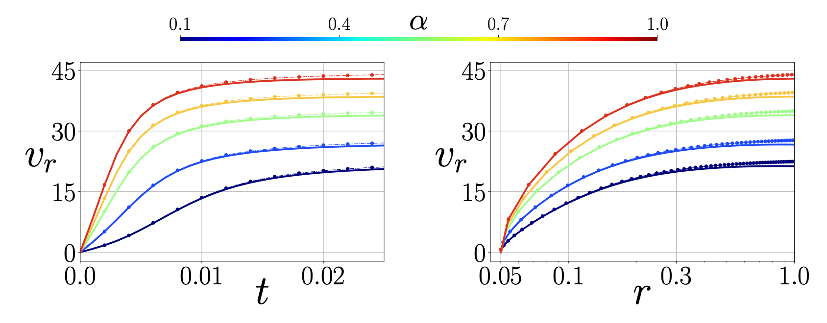
Figure 4: Comparison of trajectories obtained analytically from the inner solution (dotted lines with symbols) with the numerically solved trajectories for the complete dynamics (solid lines), of a particle starting from $r_{0}=0.05$, for different $\alpha$.

(b) Outer solution, $r\gg 1$: At large time, particles move well outside the inner layer, and we may rescale $r$ and $t$ in equation (21) such that the new scales (outer variables) are $\mathcal{O}(1)$: $t\to t/\epsilon_{o}$ and $r\to r/\delta_{o}$, for small $\epsilon_{o}$ and $\delta_{o}$. Substituting this in the equation for $r$ gives a constant $r(t)$, with no further caustics, and in fact no further activity. Thus, there is a critical radial distance $R_{0}$ above which caustics do not occur.

For completeness, we solve for the particle’s approach to this final state. Active particles and inertial particles have significantly different long-term behaviour if they start close to the vortex origin. Both active and inertial particles get thrown out to large radial distances because of the strong centrifugal force and effective centrifugal force respectively, close to the vortex. Thereafter, inertial particles keep centrifuging out and at long times, the radial acceleration becomes negligible. The drag force balances the centrifugal force and radial velocity decays as $r^{-3}$ Croor2022 . For active Hookean dimers on the other hand, if $r_{f}$ is their final radius, it is convenient to define

$$\begin{split}r(t)=r_{f}-R(t)\ ,\end{split}$$ (28)

where $r_{f}=q/\delta_{o}$ with $q,R\sim\mbox{O}(1)$ and $\delta_{o}\ll 1$. Using this in the non-dimensional form of equation (19) we get

$$\begin{split}-\ddot{R}&=\dot{R}+\frac{\delta_{o}^{3}}{q^{3}}\left(L-1\right)\left(L-\alpha\right)+\mbox{O}(\delta_{o}^{4}),\\ \dot{L}&=1-L+\frac{\delta_{o}(\alpha+1)}{q}\dot{R}+\mbox{O}(\delta_{o}^{2})\ .\end{split}$$ (29)

If we expand $R$ and $L$ in orders of $\delta_{o}$ and write

$$\begin{split}R=\sum\limits_{n=0}^{\infty}R_{n}\delta_{o}^{n}\qquad;\qquad L=\sum\limits_{n=0}^{\infty}L_{n}\delta_{o}^{n}\,\end{split},$$ (30)

the solutions to $\mbox{O}(\delta_{o}^{0})$ are

$$\begin{split}R_{0}=v_{r}^{*}(\alpha)e^{-(t-t^{*})}\qquad;\qquad L_{0}=1-(1-L^{*}(\alpha))e^{-(t-t^{*})}\ ,\end{split}$$ (31)

where $v_{r}(t=t^{*})=v_{r}^{*}$ and $L(t=t^{*})=L^{*}$. In other words, far away from the origin

$$\begin{split}r=r_{f}(\alpha)-v_{r}^{*}(\alpha)e^{-(t-t^{*})}+\mbox{O}(\delta_{o})\qquad;\qquad L=1-(1-L^{*}(\alpha))e^{-(t-t^{*})}+\mbox{O}(\delta_{o})\ .\end{split}$$ (32)

Finding the $\mbox{O}(\delta_{o})$ correction to the solution is straightforward. The equation of $R$ remains the same at this order and so does its solution. The $\mbox{O}\left(\delta_{o}\right)$ correction to the equation for $L$ is

$$\begin{split}\dot{L}_{1}&=-L_{1}+\frac{(\alpha+1)}{q}\dot{R}_{0}\,\end{split}$$ (33)

and this equation can be integrated. To $\mbox{O}(\delta_{o})$ we then have

$$\begin{split}L&=1-(1-L^{*}(\alpha))e^{-(t-t^{*})}+\left(t-t^{*}\right)\left(\alpha+1\right)\frac{v_{r}^{*}}{r_{f}}\,e^{-(t-t^{*})}+\mbox{O}(\delta_{o}^{2}),\\ r&=r_{f}-v_{r}^{*}e^{-(t-t^{*})}+\mbox{O}(\delta_{o}^{2})\ .\end{split}$$ (34)

For every particle, $r_{f}$ and the initial conditions $L^{*},v_{r}^{*}$ vary with $\alpha$. This is evident in Fig. 5 which shows the outer solution alongside the full numerical solution for different $\alpha$.

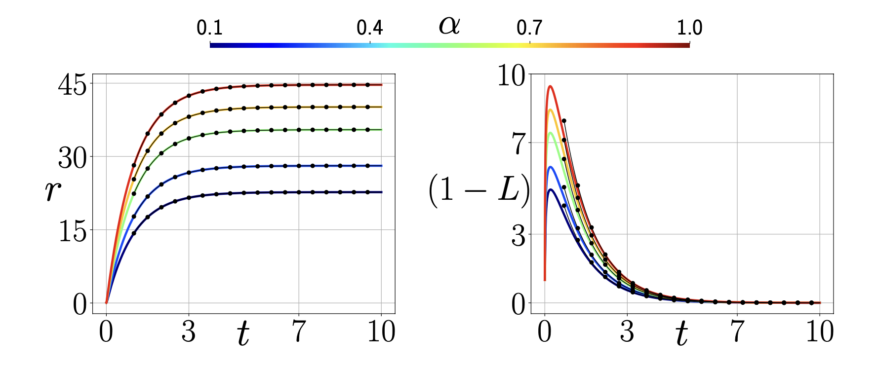
Figure 5: Comparison of the outer solution (symbols) with the complete solution (lines) for particles starting from close to the vortex ($r_{0}=0.05$).

III.3 Caustics from the distribution of final states

If two rings of particles start with initial radii $r_{01}$ and $r_{02}$ with $r_{01}<r_{02}$ and end at final radii $r_{f1}$ and $r_{f2}$ respectively, with $r_{f1}>r_{f2}$, they must have undergone caustics during their evolution. We can thus identify, from the regions of negative slope, that caustics occur in almost everywhere in the range of initial locations shown in Fig. 6.

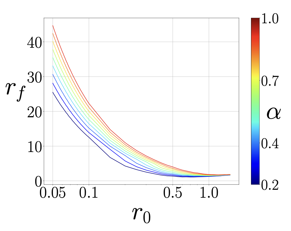
Figure 6: Average final radius for a range of initial radius, for different activity levels $\alpha$, of particles near a point vortex.

IV Caustics from the continuum limit of active particles

So far, we have obtained caustics by evolving pairs of particles close to each other and then checking if their paths cross. The initial separation between the two particles is a free parameter, and we have made sure that its choice does not affect our answers. We may confirm our findings by following an alternative approach that does not contain this free parameter. In this approach, we imagine a continuum of particles described by its velocity field $\mathbf{v}=\mathbf{v}(\mathbf{x},t)$ obeying

$$\begin{split}\frac{\tau}{\mu}d_{t}v_{i}=-\left[\frac{1}{\mu}-\frac{\tau}{\mu}\left(\alpha+1\right)\textsf{{S}}_{ik}\right]\left(v_{k}-U_{k}\right)+F_{i}+\frac{\tau}{\mu}\left(D_{t}-\beta\ell^{2}\nabla^{2}\right)U_{i}+\frac{\beta}{\mu}\sqrt{2D}\,\eta_{i}\ ,\end{split}$$ (35)

where $d_{t}\equiv\partial_{t}+v_{k}\partial_{k}$ is the time derivative convected by the particle velocity. The particle velocity field is continuous everywhere except in caustics regions and generally has a non-zero divergence since the particle flow is compressible. Caustics occur when this divergence $\mathbf{\nabla}.\mathbf{v}\to-\infty$ meibohm2d2021 . Upon defining a non-dimensional particle gradient tensor $\textsf{{Z}}=\tau\mathbf{\nabla}\mathbf{v}$, this condition translates to $\operatorname{Tr}{\textsf{{Z}}}\to-\infty$. An equation for the quantity Z follows readily from equation (35):

$$\begin{split}d_{t}\textsf{{Z}}_{ij}=&-\frac{1}{\tau}\left(\textsf{{Z}}_{ij}-\tilde{\textsf{{O}}}_{ij}+\textsf{{Z}}^{2}_{ij}\right)+\mu\partial_{j}F_{i}+\left(D_{t}-\beta\ell^{2}\nabla^{2}\right)\tilde{\textsf{{O}}}_{ij}+\frac{1}{\tau}\tilde{\textsf{{O}}}^{2}_{ij}+\beta\sqrt{2D}\,\partial_{j}\eta_{i}\\ &+\frac{\alpha+1}{2}\left[\left(\mathbf{v}-\mathbf{U}\right).\mathbf{\nabla}\tilde{\textsf{{O}}}_{ij}+\left(v_{k}-U_{k}\right)\partial_{i}\tilde{\textsf{{O}}}_{kj}+\frac{2}{\tau}\tilde{\textsf{{S}}}_{ik}\left(\textsf{{Z}}_{kj}-\tilde{\textsf{{O}}}_{kj}\right)\right],\end{split}$$ (36)

where $\tilde{\textsf{{O}}}=\tau\mathbf{\nabla}\mathbf{u}=\tau\left(\textsf{{S}}+\textsf{{A}}\right)$ is the non-dimensional fluid gradient tensor with $\tilde{\textsf{{S}}}=\tau\textsf{{S}}$ and $\tilde{\textsf{{A}}}=\tau\textsf{{A}}$ being its symmetric and anti-symmetric part respectively. The benefit of equation (36) is that it can be solved in the Lagragian frame of an individual particle and can thus predict whether a given particle will undergo caustics. Furthermore, as the field description assumes a continuum of particles everywhere in the domain, Z at a single point measures the differences in particle velocities in the neighbourhood of that point.

In the following, we identify caustics formation by active Hookean Dimers near a point vortex using both equations (35) and (36) and show that they give the same results.

Defining non-dimensional number $\lambda=\beta\tau\ell^{2}/L^{2}$ and setting $\mathbf{F},\mathbf{\eta}$ and $\lambda$ to zero, equation (35) reduces to the non-dimensional form

$$\begin{split}d_{t}v_{i}=-\left[1-\left(\alpha+1\right)\tilde{\textsf{{S}}}_{ik}\right]\left(v_{k}-U_{k}\right)+D_{t}U_{i}\ ,\end{split}$$ (37)

where $\tilde{\textsf{{S}}}$ in $x,y,z$ system takes the form

$$\begin{split}\tilde{\textsf{{S}}}_{ij}\equiv-\frac{1}{r^{2}}\left[\begin{array}[]{ccc}-\sin 2\theta&\cos 2\theta&0\\ \cos 2\theta&\sin 2\theta&0\\ 0&0&0\end{array}\right]=\tilde{\textsf{{O}}}_{ij}\ ,\end{split}$$ (38)

with $\theta=\tan^{-1}(y/x)$, everywhere except at the origin. Similarly, equation (36) becomes

$$d_{t}\textsf{{Z}}_{ij}=-\left(\textsf{{Z}}_{ij}-\tilde{\textsf{{S}}}_{ij}+\textsf{{Z}}^{2}_{ij}\right)+D_{t}\tilde{\textsf{{S}}}_{ij}+\tilde{\textsf{{S}}}^{2}_{ij}+\left(\alpha+1\right)\left[\left(\mathbf{v}-\mathbf{U}\right).\mathbf{\nabla}\tilde{\textsf{{S}}}_{ij}+\tilde{\textsf{{S}}}_{ik}\left(\textsf{{Z}}_{kj}-\tilde{\textsf{{S}}}_{kj}\right)\right]\ ,$$ (39)

where

$$\begin{split}D_{t}U_{i}=\mathbf{U}.\mathbf{\nabla}U_{i}\quad{\rm and}\quad D_{t}\tilde{\textsf{{S}}}_{ij}=\mathbf{U}.\mathbf{\nabla}\tilde{\textsf{{S}}}_{ij}.\end{split}$$ (40)

With these equations, we initialise active hookean particles at different radii and evaluate where and when they form caustics. Fig. 7 shows the time taken for different particles to form caustics starting from a radius $r_{0}$ for different values of $\alpha$. The initial velocity was taken to be $\mathbf{v}(0)=\sin(r)\mathbf{U}$. The caustics detected by the $\operatorname{Tr}{\textsf{{Z}}}\to-\infty$ (crosses) practically overlap with those obtained from computing particle trajectories (lines) and identifying overtaking events.

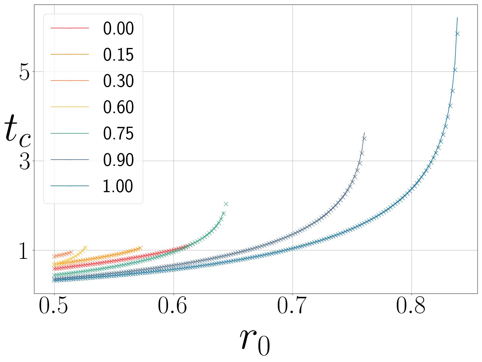
Figure 7: Caustics times for particles starting from different initial radii as calculated from equations (37) (lines) and (39) (crosses).

V Active Preferred-length dimer in a point vortex

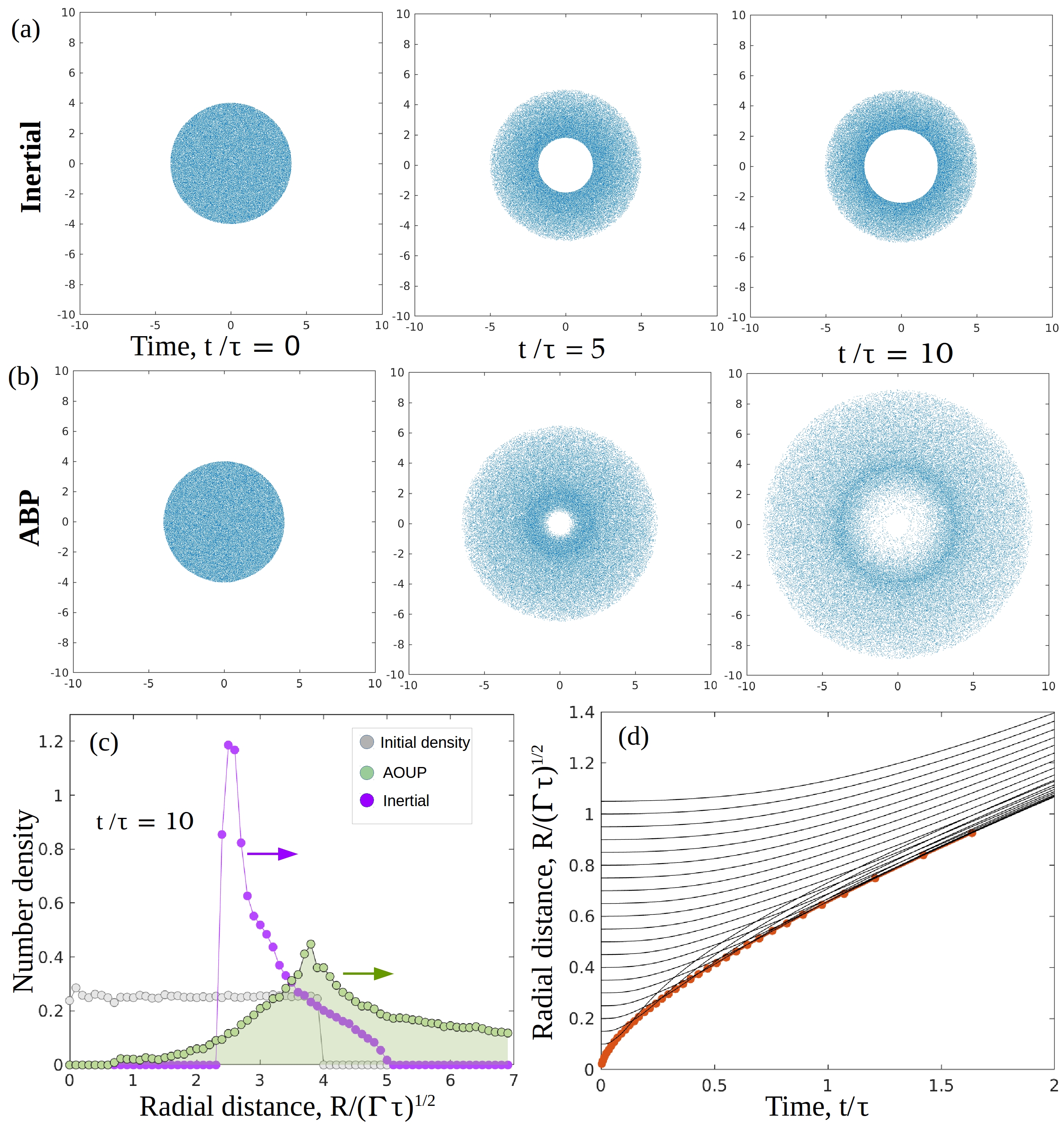
Figure 8: Centrifugation and caustics of persistent active dimers (noiseless ABP) in a point vortex: (a) & (b) show time frames of particle positions around a point vortex for inertial particles and noiseless ABP respectively, shown for $\tilde{\beta}=0.5$ and $\alpha=1.0$ in (41) - (42). (c) radial number-density of active particles (green) compared with inertial particles (purple) shown for time $10\tau$, and the number-density at $t=0$ (grey). Arrows schematically depict the radial drift of the unsteady state. (d) Intersections of adjacent trajectories marking the caustics curve (red circles) obtained for $\tilde{\beta}=0.5$, $\alpha=1.0$ and $\Delta r=0.01$.

The equations for an active dimer which has a preferred length are given by

$$\dot{\mathbf{X}} =\mathbf{U}+\beta\mathbf{w}$$ (41)

$$\dot{\mathbf{w}} =\frac{1}{\tau}(1-|\mathbf{w}|^{2})\mathbf{w}+(\alpha\textsf{{S}}+\textsf{{A}})\cdot\mathbf{w}{+{\bf f}(t)},$$ (42)

They can be recast as

$$\frac{d\mathbf{v}}{dt}-\mathbf{v}\cdot\nabla\mathbf{U}=\,(\mathbf{U}-\mathbf{v})\cdot\tilde{\tau}^{-1}$$ (43)

where $\tilde{\tau}^{-1}\equiv\frac{\textsf{{I}}}{\tau}\left(\frac{||V-U||}{\beta^{2}}-1\right)-(\alpha\,\textsf{{S}}+\textsf{{A}}\,)$. The non-dimensional equations with $R=\sqrt{\tilde{\Gamma}\tau}$ and $T=\tau$, in cylindrical polar coordinates become

$$\tilde{\beta}^{2}\frac{d^{2}r}{dt^{2}} =\tilde{\beta}^{2}r\left(\frac{d\theta}{dt}\right)^{2}+\frac{dr}{dt}\left\{2\frac{d\theta}{dt}-\left(\frac{dr}{dt}\right)^{2}-r^{2}\left(\frac{d\theta}{dt}\right)^{2}+\tilde{\beta}^{2}-\frac{1}{r^{2}}\right\}+\frac{\tilde{\beta}^{2}\alpha}{r^{3}}$$

$$-\frac{\tilde{\beta}^{2}(1+\alpha)}{r}\frac{d\theta}{dt},$$ (44)

$$\tilde{\beta}^{2}r\frac{d^{2}\theta}{dt^{2}} =-2\tilde{\beta}^{2}\frac{d\theta}{dt}\frac{d\theta}{dt}+\left(r\frac{d\theta}{dt}-\frac{1}{r}\right)\left\{2\frac{d\theta}{dt}-\left(\frac{dr}{dt}\right)^{2}-r^{2}\left(\frac{d\theta}{dt}\right)^{2}+\tilde{\beta}^{2}-\frac{1}{r^{2}}\right\}$$

$$-\frac{\tilde{\beta}^{2}(1+\alpha)}{r^{2}}\frac{dr}{dt},$$ (45)

where $\tilde{\beta}\equiv\beta\sqrt{\tau/{\tilde{\Gamma}}}$ is the non-dimensional motility. These may be recast as a system of first-order equations as

$$\frac{dr}{dt} =v_{r},$$ (46)

$$\tilde{\beta}^{2}\frac{dv_{r}}{dt} =\tilde{\beta}^{2}r\omega^{2}+v_{r}\left\{2\omega-{v_{r}}^{2}-r^{2}{\omega}^{2}+\tilde{\beta}^{2}-\frac{1}{r^{2}}\right\}+\frac{\tilde{\beta}^{2}\alpha}{r^{3}}-\frac{\tilde{\beta}^{2}(1+\alpha)\,\omega}{r},$$ (47)

$$\frac{d\theta}{dt} =\omega,$$ (48)

$$\tilde{\beta}^{2}\frac{d\omega}{dt} =-\frac{2\tilde{\beta}^{2}\,v_{r}\,\omega}{r}+\left(\omega-\frac{1}{r^{2}}\right)\left\{2\omega-{v_{r}}^{2}-r^{2}{\omega}^{2}+\tilde{\beta}^{2}-\frac{1}{r^{2}}\right\}-\frac{\tilde{\beta}^{2}(1+\alpha)\,v_{r}}{r^{3}}.$$ (49)

Similar to the active Hookean dimer case, we numerically explore the dynamics of a suspension of active preferred-length dimers in a point vortex, by integrating equations (41) - (42) with random initial orientations uniformly distributed on a disk of radius $4\sqrt{\tilde{\Gamma}\tau}$. We find persistent centrifugation, similar to that seen for bacteria in a vortex Sokolov2016 . In Figure 8, we compare this effective centrifugation of active particles with that of their inertial counterparts, for $\tilde{\beta}=0.5$ and $\alpha=1.0$ for various time frames. The radial number density does not have a steady state, and particles keep drifting radially outward on average, akin to inertial particles. A crucial distinction is the display of sharper caustics by inertial particles, with complete expulsion of particles within a ring that expands radially outwards with a velocity that asymptotically goes to $0$ as $r\to\infty$ Croor2015 . In contrast, the radial drift of active particles approaches a constant velocity for $r\gg 1$. The outer solution from the asymptotic analysis of (46) - (49) predicts this constant radial velocity to be the non-dimensional motility $\tilde{\beta}$ of a “free” particle, consistent with the linearity of the rays at late times in Fig 8 (d). Note that this velocity is independent of the shape-dependent flow coupling $\alpha$. We also find a caustics curve in the $r-t$ plane by measuring the intersection of adjacent trajectories with $\Delta r=0.01$. The caustics radius for ABPs depends on both $\alpha$ and $\tilde{\beta}$. For a fixed $\tilde{\beta}=1.0$, we get the caustics phase in the $r-\alpha$ plane, by measuring the divergence of crossing time, similar to the AOUP case. We compare this phase of dimer with the rigid spheroid of changing $\alpha$ that depends on the eccentricity of the spheroid, with $\alpha=0$ being the spherical limit. Note that rigid spherical microswimmers Stark2012 ; Stark2016 in vortical flow can also display caustics, depending on whether $\tilde{\beta}$ is large or small.

VI Pseudospectral Direct Numerical Simulations (DNS) of Active Dimer in Turbulence

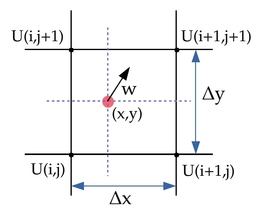
Figure 9: Bilinear interpolation scheme to evaluate fluid fields in the continuous domain of particle dynamics.

The two-dimensional Navier-Stokes equation in the stream function $\psi$ and vorticity $\omega$ formulation in the Fourier space is

$$\hat{\psi}=-\hat{\omega}/k^{2},$$ (50)

$$\frac{\partial\hat{\omega}}{\partial t}=i(k_{x}\widehat{u_{x}\omega}+k_{y}\widehat{u_{y}\omega})-(\nu k^{2}+\mu)\hat{\omega}+\hat{f},$$ (51)

where $\hat{.}$ is the Fourier transform, $(u_{x},u_{y})=(-\partial_{y}\psi,\partial_{x}\psi)$, and $\hat{f}$ is the curl of the forcing term in Fourier space. In two dimensions, the inverse cascade feeds energy into long wavelengths, which we avoid by including the Ekman friction $\mu$ Boffetta2012 , in addition to the viscous dissipation $\nu$. We solve the spectral DNS in $512\times 512$ numerical grids with a $2\pi$ periodic domain. We initialize the flow with a Taylor-Green vortex array

$$u_{x}=\frac{1}{2}\sin(x)\cos(y)\exp{(-2\nu t)}, u_{y}=-\frac{1}{2}\cos(x)\sin(y)\exp{(-2\nu t)},$$ (52)

which gives the vorticity field $\omega(x,y)=\sin x\sin y$, at $t=0$. We take kinematic viscosity $\nu=5\times 10^{-5}\,\text{m}^{2}\text{s}^{-1}$, Ekman friction coefficient $\mu=0.01\,\text{s}^{-1}$ and the real space forcing $f=f_{0}k_{f}\cos(k_{f}x)$ with forcing wavenumber $k_{f}=3\,\text{m}^{-1}$ and $f_{0}=0.1\,\text{m s}^{-2}$. Since the flow in $x$ and $y$ directions are coupled, the forcing wavenumber along $x$ suffices to drive the flow in both directions in wavenumber space.

The Fourier and inverse Fourier transforms at each time step were carried out using the C library fftw3. To eliminate aliasing errors, a third of the large wavenumber Fourier modes were set to zero at each time step Boffetta2012 . At each time step the fourier transform of forcing $f=f_{0}k_{f}\cos(k_{f}x)$ is added to 51 which drives the fluid. This at long enough time scales leads to a steady state turbulence, after which we introduce self propelled particles with uniformly random positions and orientations, and thereafter the particle and fluid evolves simultaneously. We calculate the fluid dynamics leading to the steady state turbulence only once, and use it as an initial condition for the DNS in subsequent simulations. The dynamics of particles happen in a continuous space, whereas fluid dynamics happen on the numerical grid points separated by $\Delta x=\Delta y=2\pi/512$ [see Figure 9]. Particle dynamics at position $(x,y)$ require the velocity field $\mathbf{U}$ and the tensor field $\nabla\mathbf{U}$ at $(x,y)$. We use bilinear interpolation to get the value of $\mathbf{U}=(u_{x},u_{y})$ and $\mathbf{\nabla U}$ at a point $(x,y)$ lying in a grid specified by the indices $(i,j)$, $(i+1,j)$, $(i,j+1)$, $(i+1,j+1)$, which can be written in the matrix form to leading order in $\Delta x,\Delta y$

$$u_{x}(x,y)=\frac{1}{\Delta x\Delta y}\begin{pmatrix}(i+1)\Delta x-x&x-i\Delta x\end{pmatrix}\begin{pmatrix}u_{x}(i,j)&u_{x}(i+1,j)\\ u_{x}(i,j+1)&u_{x}(i+1,j+1)\end{pmatrix}\begin{pmatrix}(j+1)\Delta y-y\\ y-j\Delta y\end{pmatrix},$$ (53)

where $i,j=1,2..,511$. For $i,j=512$ we take $i+1,j+1=1$ to satisfy periodic boundary conditions. We treat other field components by similar interpolation. We evolve the particles [Eqn. (41) - (42)] and the fields [Eqn. (50)-(51)] using the Runge-Kutta-4 algorithm with the time step $\Delta t=10^{-3}$.

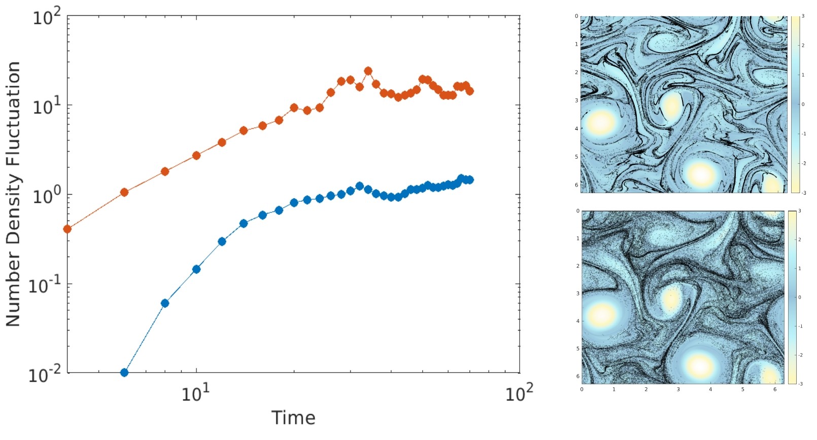
Figure 10: Number-density fluctuations: The fluctuations saturate as a function of time as the particulate structure evolves from a uniformly random state to exhibiting caustics. Red and blue curves correspond to $\ell^{2}/w_{0}^{2}=2\times 10^{3}$ and $\ell^{2}/w_{0}^{2}=0$ respectively. The activity $\beta/\kappa=236$ in both cases. The top and bottom panels on the right correspond to the top and bottom curves on the left respectively.

VII Number density fluctuation, clustering and collisions

Local number-density fluctuations can be used as a statistical measure for the intensity of caustic induced clustering. The space is numerically discretized into $N\times N$ cells such that there is on an average 1 particle per cell in the initial uniformaly random state

$${\Delta\rho_{ij}}^{2}=\frac{1}{N^{2}}\sum_{i,j}(\rho_{ij}-1)^{2}.$$ (54)

Here, $i,j$ are the cell index corresponding to a given spatial location. The initial state itself contributes a residual density fluctuation which we subtract, to obtain purely caustics-induced clustering.

To measure collisions we find pairs of particles whose trajectories intersect within the numerical time step $\Delta t=10^{-3}$, as shown in 11. Such particles are colored red in Supplementary Video 5; where find that the regions with high number-density coincides with the crossing of particle trajectories.

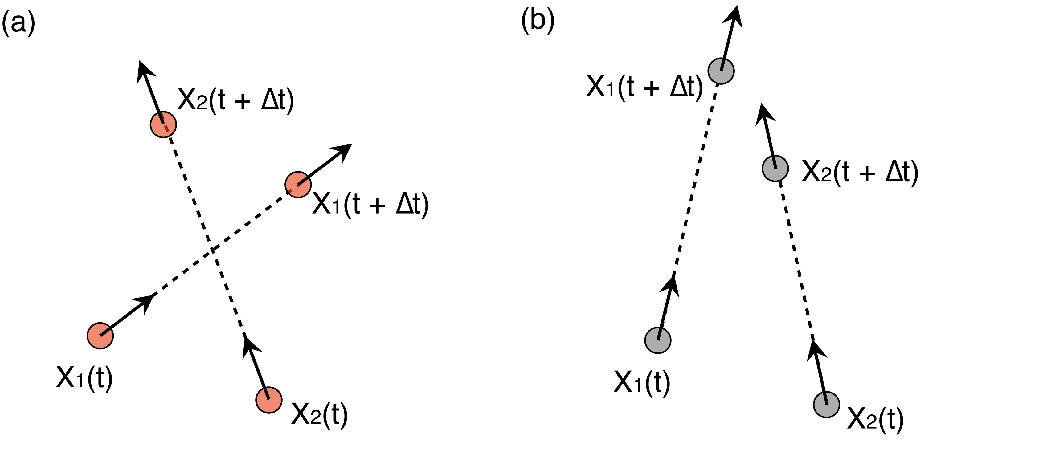
Figure 11: Collisions: A schematic of (a) colliding (red) and (b) non-colliding (grey) pairs of particles, where the intersection of paths within the numerical time step $\Delta t$ marks the collision event.

References

- (1) M. Pinsky and A. Khain, “Turbulence effects on droplet growth and size distribution in clouds—a review,” Journal of Aerosol Science, vol. 28, no. 7, pp. 1177–1214, 1997.
- (2) H. J. S. Fernando, D. Zajic, S. Di Sabatino, R. Dimitrova, B. Hedquist, and A. Dallman, “Flow, turbulence, and pollutant dispersion in urban atmospheres,” Physics of Fluids, vol. 22, no. 5, p. 051301, 2010.
- (3) P. W. Boyd, H. Claustre, M. Levy, D. A. Siegel, and T. Weber, “Multi-faceted particle pumps drive carbon sequestration in the ocean,” Nature, vol. 568, pp. 327–335, 2019.
- (4) K. Samborska, S. Poozesh, A. Barańska, M. Sobulska, A. Jedlińska, C. Arpagaus, N. Malekjani, and S. M. Jafari, “Innovations in spray drying process for food and pharma industries,” Journal of Food Engineering, vol. 321, p. 110960, 2022.
- (5) G. Boffetta, F. De Lillo, and A. Gamba, “Large scale inhomogeneity of inertial particles in turbulent flows,” Physics of Fluids, vol. 16, no. 4, pp. L20–L23, 2004.
- (6) M. R. Maxey and J. J. Riley, “Equation of motion for a small rigid sphere in a nonuniform flow,” The Physics of Fluids, vol. 26, no. 4, pp. 883–889, 1983.
- (7) M. R. Maxey and S. Corrsin, “Gravitational settling of aerosol particles in randomly oriented cellular flow fields,” Journal of Atmospheric Sciences, vol. 43, no. 11, pp. 1112 – 1134, 1986.
- (8) S. Ravichandran and R. Govindarajan, “Caustics and clustering in the vicinity of a vortex,” Physics of Fluids, vol. 27, no. 3, p. 033305, 2015.
- (9) M. Wilkinson and B. Mehlig, “Caustics in turbulent aerosols,” Europhysics Letters (EPL), vol. 71, pp. 186–192, jul 2005.
- (10) P. Deepu, S. Ravichandran, and R. Govindarajan, “Caustics-induced coalescence of small droplets near a vortex,” Phys. Rev. Fluids, vol. 2, p. 024305, Feb 2017.
- (11) E. Lauga and T. R. Powers, “The hydrodynamics of swimming microorganisms,” Reports on progress in physics, vol. 72, no. 9, p. 096601, 2009.
- (12) E. J. Buskey, “Components of mating behavior in planktonic copepods,” Journal of Marine Systems, vol. 15, no. 1, pp. 13–21, 1998.
- (13) G. Basterretxea, J. S. Font-Muñoz, and I. Tuval, “Phytoplankton orientation in a turbulent ocean: A microscale perspective,” Frontiers in Marine Science, vol. 7, 2020.
- (14) J. S. Guasto, R. Rusconi, and R. Stocker, “Fluid mechanics of planktonic microorganisms,” Annual Review of Fluid Mechanics, vol. 44, no. 1, pp. 373–400, 2012.
- (15) R. Monthiller, A. Loisy, M. A. R. Koehl, B. Favier, and C. Eloy, “Surfing on turbulence: A strategy for planktonic navigation,” Phys. Rev. Lett., vol. 129, p. 064502, Aug 2022.
- (16) S. A. Berman, J. Buggeln, D. A. Brantley, K. A. Mitchell, and T. H. Solomon, “Transport barriers to self-propelled particles in fluid flows,” Phys. Rev. Fluids, vol. 6, p. L012501, Jan 2021.
- (17) W. M. Durham, E. Climent, M. Barry, F. De Lillo, G. Boffetta, M. Cencini, and R. Stocker, “Turbulence drives microscale patches of motile phytoplankton,” Nature Communications, vol. 4, no. 2148, 2013.
- (18) K. Gustavsson, F. Berglund, P. R. Jonsson, and B. Mehlig, “Preferential sampling and small-scale clustering of gyrotactic microswimmers in turbulence,” Phys. Rev. Lett., vol. 116, p. 108104, Mar 2016.
- (19) A. Abelson and M. Denny, “Settlement of marine organisms in flow,” Annual Review of Ecology and Systematics, vol. 28, no. 1, pp. 317–339, 1997.
- (20) D. Krishnamurthy, H. Li, F. B. du Rey, P. Cambournac, A. G. Larson, E. Li, and M. Prakash, “Scale-free vertical tracking microscopy,” Nature Methods, vol. 17, pp. 1040–1051, Aug. 2020.
- (21) N. Mousavi, J. Qiu, B. Mehlig, L. Zhao, and K. Gustavsson, “Efficient survival strategy for zooplankton in turbulence,” 2023.
- (22) T. Pedley and J. O. Kessler, “Hydrodynamic phenomena in suspensions of swimming microorganisms,” Annual Review of Fluid Mechanics, vol. 24, no. 1, pp. 313–358, 1992.
- (23) C. Torney and Z. Neufeld, “Transport and aggregation of self-propelled particles in fluid flows,” Phys. Rev. Lett., vol. 99, p. 078101, Aug 2007.
- (24) C. Zhan, G. Sardina, E. Lushi, and L. Brandt, “Accumulation of motile elongated micro-organisms in turbulence,” Journal of Fluid Mechanics, vol. 739, p. 22–36, 2014.
- (25) J. O. Kessler, “Hydrodynamic focusing of motile algal cells,” Nature, vol. 313, pp. 218–220, Jan. 1985.
- (26) A. Genin, “Bio-physical coupling in the formation of zooplankton and fish aggregations over abrupt topographies,” Journal of Marine Systems, vol. 50, no. 1, pp. 3–20, 2004. The Role of Biophysical Coupling in Concentrating Marine Organisms Around Shallow Topographies.
- (27) S. Yazdi and A. M. Ardekani, “Bacterial aggregation and biofilm formation in a vortical flow,” Biomicrofluidics, vol. 6, no. 4, p. 044114, 2012.
- (28) A. Sokolov and I. S. Aranson, “Rapid expulsion of microswimmers by a vortical flow,” Nature Communications, vol. 7, no. 11114, 2016.
- (29) H. Stark, “Swimming in external fields,” The European Physical Journal Special Topics, vol. 225, p. 2369–2387, 2016.
- (30) E. Lushi and P. M. Vlahovska, “Periodic and chaotic orbits of plane-confined micro-rotors in creeping flows,” Journal of Nonlinear Science, vol. 25, p. 1111–1123, October 2015.
- (31) N. Oppenheimer, D. B. Stein, and M. J. Shelley, “Rotating membrane inclusions crystallize through hydrodynamic and steric interactions,” Phys. Rev. Lett., vol. 123, p. 148101, Oct 2019.
- (32) J.-A. Arguedas-Leiva and M. Wilczek, “Microswimmers in an axisymmetric vortex flow,” New Journal of Physics, vol. 22, p. 053051, may 2020.
- (33) R. Chajwa, N. Menon, and S. Ramaswamy, “Kepler orbits in pairs of disks settling in a viscous fluid,” Phys. Rev. Lett., vol. 122, p. 224501, Jun 2019.
- (34) A. Bolitho, R. Singh, and R. Adhikari, “Periodic orbits of active particles induced by hydrodynamic monopoles,” Phys. Rev. Lett., vol. 124, p. 088003, Feb 2020.
- (35) R. Chajwa, N. Menon, S. Ramaswamy, and R. Govindarajan, “Waves, algebraic growth, and clumping in sedimenting disk arrays,” Phys. Rev. X, vol. 10, p. 041016, Oct 2020.
- (36) K. Son, F. Menolascina, and R. Stocker, “Speed-dependent chemotactic precision in marine bacteria,” Proceedings of the National Academy of Sciences, vol. 113, no. 31, pp. 8624–8629, 2016.
- (37) M. Lisicki, M. F. Velho Rodrigues, R. E. Goldstein, and E. Lauga, “Swimming eukaryotic microorganisms exhibit a universal speed distribution,” eLife, vol. 8, p. e44907, jul 2019.
- (38) H. L. Fuchs and G. P. Gerbi, “Seascape-level variation in turbulence- and wave-generated hydrodynamic signals experienced by plankton,” Progress in Oceanography, vol. 141, pp. 109–129, 2016.
- (39) E. Fodor, C. Nardini, M. E. Cates, J. Tailleur, P. Visco, and F. van Wijland, “How far from equilibrium is active matter?,” Phys. Rev. Lett., vol. 117, p. 038103, Jul 2016.
- (40) P. Romanczuk, M. Bär, W. Ebeling, B. Lindner, and L. Schimansky-Geier, “Active brownian particles,” The European Physical Journal Special Topics, vol. 202, no. 1, pp. 1–162, 2012.
- (41) A. Maitra, P. Srivastava, M. Rao, and S. Ramaswamy, “Activating membranes,” Physical review letters, vol. 112, no. 25, p. 258101, 2014.
- (42) G. B. Jeffery and L. N. G. Filon, “The motion of ellipsoidal particles immersed in a viscous fluid,” Proceedings of the Royal Society of London. Series A, Containing Papers of a Mathematical and Physical Character, vol. 102, no. 715, pp. 161–179, 1922.
- (43) S. G. Prasath, V. Vasan, and R. Govindarajan, “Accurate solution method for the maxey-riley equation, and the effects of basset history,” Journal of Fluid Mechanics, vol. 868, pp. 428–460, 2019.
- (44) C. M. Bender and S. A. Orzag, Advanced mathematical methods for scientists and engineers i: Asymptotic methods and perturbation theory. New York: Springer, 1999.
- (45) J. Eggers and M. A. Fontelos, Singularities: Formation, Structure, and Propagation. Cambridge Texts in Applied Mathematics, Cambridge University Press, 2015.
- (46) M. et al., “Paths to caustic formation in turbulent aerosols,” Physical Review Fluids, vol. 6, no. 6, p. L062302, 2021.
- (47) W. M. Durham, E. Climent, and R. Stocker, “Gyrotaxis in a steady vortical flow,” Phys. Rev. Lett., vol. 106, p. 238102, Jun 2011.
- (48) J. Eaton and J. Fessler, “Preferential concentration of particles by turbulence,” International Journal of Multiphase Flow, vol. 20, pp. 169–209, 1994.
- (49) G. Boffetta and R. E. Ecke, “Two-dimensional turbulence,” Annual Review of Fluid Mechanics, vol. 44, no. 1, pp. 427–451, 2012.
- (50) J. R. Picardo, D. Vincenzi, N. Pal, and S. S. Ray, “Preferential sampling of elastic chains in turbulent flows,” Phys. Rev. Lett., vol. 121, p. 244501, Dec 2018.
- (51) S. Ravichandran and R. Govindarajan, “Waltz of tiny droplets and the flow they live in,” Physical Review Fluids, vol. 7, no. 11, p. 110512, 2022.
- (52) A. Zöttl and H. Stark, “Nonlinear dynamics of a microswimmer in poiseuille flow,” Phys. Rev. Lett., vol. 108, p. 218104, May 2012.