Unifying Safety Approaches for Stochastic Systems: From Barrier Functions to Uncertain Abstractions via Dynamic Programming

Abstract

Providing safety guarantees for stochastic dynamical systems has become a central problem in many fields, including control theory, machine learning, and robotics. Existing methods either employ Stochastic Barrier Functions (SBFs) or rely on numerical approaches based on abstractions. While SBFs are analogous to Lyapunov functions to prove (probabilistic) set invariance, abstraction-based approaches approximate the stochastic system into a finite model for the computation of safety probability bounds. In this paper, we offer a new perspective on these seemingly different methods. We show that both these approaches arise as approximations of a stochastic dynamic programming problem. Such a new and unifying perspective allows us to formally show the correctness of both approaches, characterise their convergence and optimality properties, and examine advantages and disadvantages of each. Our analysis reveals that abstraction-based methods can provide more accurate certificates of safety, but generally at a higher computational cost. We conclude the article with a discussion that highlights possible future directions.

Finite Abstraction, Barrier Function, Probabilistic Safety, Robustness, Stochastic Systems

1 Introduction

In the age of autonomous systems, control systems have become ubiquitous, playing a pivotal role in safety-critical applications. Examples span from autonomous vehicles [1] to medical robots [2], where the consequences of bad decisions are not only costly but can also prove fatal. A common characteristic of these systems is the inherent complexity and nonlinearity of the dynamics that are subject to uncertainty due to physics (e.g., sensor or actuation noise) or algorithms (e.g., black-box controllers or perception). Consequently, the question, how to ensure the safety of stochastic control systems? has emerged as a central research topic in various disciplines, including control theory, machine learning, formal methods, and robotics [3, 4, 5].

Safety for a stochastic system generalizes the standard notion of stochastic stability [5]. It is defined as the probability that the system does not exhibit unsafe behavior, i.e., that with high probability the first exit time from a safe set is greater than a given threshold or infinite. As exact computation of the safety probability is generally infeasible even in the case of stochastic systems with linear dynamics, existing formal approaches rely on under-approximations, with the two most-commonly employed approaches being stochastic barrier functions (SBFs) [6, 4] and abstraction-based methods [7, 8]. Similar to Lyapunov functions for stability, stochastic barrier functions are energy-like functions that allow one to lower bound the probability of a stochastic system remaining within a given set. On the other hand, abstraction-based methods abstract the original system into a finite, discrete-space stochastic process, generally a variant of a Markov chain, for which efficient algorithms that compute safety probability exist [9, 10, 11, 12]. A fundamental component of the abstraction process is the computation of the abstraction error, which can be used to formally bound the safety probability for the original system.

This paper presents a unified treatment of safety for discrete-time continuous-space stochastic systems under the framework of dynamic programming (DP), bridging the gap between SBFs and abstraction-based methods. While traditionally seen as distinct approaches, with SBFs typically derived from super-martingale conditions [5], this work seeks to harmonize these concepts to provide a more comprehensive perspective on safety verification of stochastic systems. We first show that, for this class of systems, the safety probability can be computed via DP and that there always exists a deterministic Markov policy (strategy) that optimizes this probability. Then, we show that both SBFs and abstraction-based methods arise as an approximation of this DP. In particular, for SBFs we show that existing bounds can be obtained by over-approximating the indicator function of the unsafe set with a barrier function, i.e., a non-negative function that is greater than one in the unsafe set. In contrast, existing approaches that perform abstractions to (uncertain) Markov process arise as piecewise-constant over- and under-approximations of the defined DP.

Viewing both SBF and abstraction-based methods as approximations for a DP problem has several advantages: (i) it gives a unified treatment of safety for stochastic systems, (ii) it allows us to establish formal bounds and guarantees on the precision and correctness of these approaches, and (iii) it enables us to fairly compare these methods and highlight their strengths and weaknesses. Specifically, we show that abstraction-based methods often return tighter bounds on the safety probability compared to SBFs, and it generally comes at the cost of an increased computation effort.

The paper is organized as follows. In Section 2, we introduce the class of systems we consider and formally define probabilistic safety. In Section 3, we define Stochastic Barrier Functions (SBFs). We present abstraction-based methods in Section 4. Finally, in Section 5, we analyze strengths and weaknesses of each method. We conclude the paper with Section 6, where we highlight important open research questions. We provide all the proofs in Section 7.

2 Probabilistic Safety for Discrete-Time Stochastic Processes

Consider a discrete-time controlled stochastic system described by the following stochastic difference equation:

$$\mathbf{x}[k+1]=F(\mathbf{x}[k],\mathbf{u}[k],\mathbf{v}[k])$$ (1)

where $\mathbf{x}[k]$ is the state of the system at time $k$ taking values in $X\subseteq\mathbb{R}^{n_{x}}$, $\mathbf{u}[k]\in U\subset\mathbb{R}^{n_{u}}$ denotes the control or action at time $k$ for $U$ being a compact set, and $\mathbf{v}[k]$ is an independent random variable distributed according to a time-invariant distribution $p(v)$ over an uncertainty space $V\subseteq\mathbb{R}^{n_{v}}$. Sets $X$, $U$, and $V$ are all assumed to be appropriately measurable sets. $F:X\times U\times V\to X$ is a possibly non-linear function representing the one-step dynamics. System (1) represents a general model of nonlinear controlled stochastic system. For instance, this model includes stochastic difference equations with additive or multiplicative noise as well as stochastic dynamical systems with neural networks in the loop [3, 13].

Definition 1 (Policy).

A feedback policy (or strategy) $\pi=(\pi_{0},\pi_{1},...)$ for System (1) is a sequence of possibly random and history-dependent universally measurable functions $\pi_{k}:X^{k+1}\to\mathcal{P}(U)$, where $\mathcal{P}(U)$ is the set of probability measures over $U$. Let $p_{u_{k}}$ denote a universally measurable kernel such that $p_{u_{k}}(\pi_{k}(x_{0},...,x_{k})\in U)=1$. Plicy $\pi$ is called deterministic if for each $k$ and $(x_{0},...x_{k})$, $p_{u_{k}}$ assigns mass one to some $u\in U$. If for each $k$, $\pi_{k}$ is only parametrized by $x_{k},$ $\pi$ is a Markov policy. A policy is stationary if, for every $k_{1},k_{2}\in\mathbb{N}$, it holds that $\pi_{k_{1}}=\pi_{k_{2}},$ in which case, with an abuse of notation, we use $\pi$ to denote any of these functions. The set of all policies is denoted by $\Pi,$ while the set of deterministic Markov policies by $\Pi^{M,D}$.

For a given initial condition $x_{0},$ a time horizon $H\in\mathbb{N}$, and a policy $\pi=(\pi_{0},...,\pi_{H-1})$, ${\mathbf{{x}}}[k]$ is a stochastic process with a well defined probability measure $P$ generated by the noise distribution $p(v)$ [14, Proposition 7.45] such that for measurable sets $X_{0},X_{k+1}\subseteq X$, it holds that

$$\begin{split}&P({\mathbf{x}}[0]\in X_{0}\mid\mathbf{u}[0]=a)=\mathbbm{1}(x_{0},X_{0}),\\ &P({\mathbf{x}}[k+1]\in X_{k+1}\mid{\mathbf{x}}[k]=x,\mathbf{u}_{k}=a)\\ &\hskip 85.35826pt:=\int_{V}\mathbbm{1}(F(x,v,a),X_{k+1})p(v)dv\\ &\hskip 85.35826pt:=T(X_{k+1}\mid x_{k},a)dx,\end{split}$$

where

$$\mathbbm{1}(x_{k},X_{k})=\begin{cases}1&\text{if }x_{k}\in X_{k}\\ 0&\text{otherwise}\end{cases}$$

is the indicator function. We refer to $T(X_{k+1}\mid x_{k},a)$ as the stochastic kernel of System (1), and we assume that for each measurable $X_{j}\subseteq X,$ $x\in X,a\in U,\,T(X_{j}\mid x,a)$ is Lipschitz continuous in both $x$ and $a$.

2.1 Probabilistic Safety

For a given policy $\pi$ and a time horizon $H\in\mathbb{N}$, probabilistic safety is defined as the probability that ${\mathbf{x}}[k]$ stays within a measurable safe set $X_{\mathrm{s}}\subseteq X$ for the next $H$ time steps. That is, the first exit time from $X_{s}$ is greater than $H.$

Definition 2 (Probabilistic Safety).

Given a policy $\pi,$ safe set $X_{\mathrm{s}}\subset X$, time horizon $H\in\mathbb{N}$, and initial set of states $X_{0}\subseteq X_{\mathrm{s}}$, probabilistic safety is defined as

$$P_{\mathrm{s}}(X_{\mathrm{s}},X_{0},H\mid\pi)=\\ \inf_{x_{0}\in X_{0}}P(\forall k\in[0,H],{{\mathbf{x}}}[k]\in X_{\mathrm{s}}\mid\mathbf{x}[0]=x_{0},\pi).$$

Probabilistic safety and its equivalent dual probabilistic reachability are widely used to certify the safety of a dynamical system [15] and represent a generalization of the notion of invariance that is commonly employed for analysis of deterministic systems [16].

Remark 1.

Note that, in Definition 2, we only consider a finite-horizon $H$. This is without lost of generality. In fact, for an infinite horizon, either there is a sub-region of $X_{\mathrm{s}}$ from which the system does not exit, in which case $P_{\mathrm{s}}$ is simply the probability of eventually reaching this region while being safe, or $P_{\mathrm{s}}=0$ as in the case that $\mathbf{v}$ is additive and has unbounded support, e.g., a Gaussian distribution.

In the rest of this section, we show that, to compute a policy that maximizes probabilistic safety, it is sufficient to restrict to deterministic Markov policies. To that end, we first show that $P_{\mathrm{s}}$ can be characterized as the solution of a DP problem. In particular, for $k\in\{H,H-1,\ldots,0\}$ and $X_{\mathrm{u}}:=X\setminus X_{\mathrm{s}}$, consider value functions $V^{*}_{k}:X\to[0,1]$ defined recursively (backwardly in time) as:

$$V^{*}_{H}(x)=\mathbbm{1}(x,X_{\mathrm{u}}),$$ (2)

$$V^{*}_{k}(x)=\inf_{a\in U}\Big{(}\mathbbm{1}(x,X_{\mathrm{u}})+\mathbbm{1}(x,X_{\mathrm{s}})\,\mathbb{E}_{x^{\prime}\sim T(\cdot\mid x,a)}[V^{*}_{k+1}(x^{\prime})]\Big{)},$$ (3)

where notation ${x^{\prime}\sim T(\cdot\mid x,a)}$ means that $x^{\prime}$ is distributed according to $T(\cdot\mid x,a)$. Intuitively, at each time step $k$, $V^{*}_{k}$ selects the (deterministic) action that minimizes the probability of reaching a state from which the system may reach $X_{\mathrm{u}}$ in the next $H-k$ time steps. Consequently, by propagating $V^{*}_{k}$ backward over time, we compute the probability of reaching $X_{\mathrm{u}}$ in the future. The following theorem guarantees that $\sup_{\pi\in\Pi}P_{\mathrm{s}}(X_{\mathrm{s}},x_{0},H\mid\pi)$ is equal to $1-V^{*}_{0}(x_{0})$. Note that while $\Pi$ also includes history-dependent random policies, in obtaining $V_{0}^{*}$ via (2)-(3), we only consider deterministic Markov policies.

Theorem 1.

For an initial state $x_{0}\in X_{\mathrm{s}}$, it holds that

$$\sup_{\pi\in\Pi}P_{\mathrm{s}}(X_{\mathrm{s}},x_{0},H\mid\pi)=1-V^{*}_{0}(x_{0}).$$

A straightforward consequence of Theorem 1 is Corollary 1, which guarantees that deterministic Markov deterministic policies are optimal.

Corollary 1.

It holds that

$$\sup_{\pi\in\Pi}P_{\mathrm{s}}(X_{\mathrm{s}},x_{0},H\mid\pi)=\sup_{\pi\in\Pi^{M,D}}P_{\mathrm{s}}(X_{\mathrm{s}},x_{0},H\mid\pi).$$

Furthermore, for every $\pi\in\Pi^{M,D}$, it holds that

$$P_{\mathrm{s}}(X_{\mathrm{s}},x_{0},H\mid\pi)=1-V_{0}^{\pi}(x_{0}),$$

where $V_{0}^{\pi}(x_{0})$ is defined recursively as

$$V^{\pi}_{H}(x)=\mathbbm{1}(x,X_{\mathrm{u}}),$$ (4)

$$V_{k}^{\pi}(x)=\mathbbm{1}(x,X_{\mathrm{u}})+\mathbbm{1}(x,X_{\mathrm{s}})\,\mathbb{E}_{x^{\prime}\sim T(\cdot\mid x,\pi_{k}(x))}[V^{\pi}_{k+1}(x^{\prime})].$$ (5)

Theorem 1 and Corollary 1 guarantee that in order to synthesize optimal policies, it is enough to consider deterministic Markov policies, and these policies can be computed via DP.

We should stress that without the assumptions made in this paper (compactness of $U$, continuity of $T$, and measurability of the various sets), $V^{*}_{k}$ may not be measurable and the infimum in $U$ in (3) may not be attained. In that case, the integrals in the expectations in (3)-(5) have to be intended as outer integrals [14]. However, under the assumptions in this paper, the expectations in the above DP are well-defined and a universally measurable deterministic Markov optimal policy exists [14], i.e., the $\inf$ is attainable for every point in the state space by a universally measurable function. However, even if $V^{*}_{0}$ and $V^{\pi}_{0}$ are well-defined, computation of (3) is infeasible in practice due to the need to solve uncountably many optimization problems. Thus, computing $P_{\mathrm{s}}$ requires approximations.

In what follows, we consider the two dominant approaches in the literature that (with certified error bounds) compute probabilistic safety and synthesize policies for System (1), namely, stochastic barrier functions (SBFs) and abstraction-based methods. We show that both approaches arise as over-approximations of the value functions $V^{\pi}_{k}$. Such a unified framework provides a basis for a fair comparison of these approaches, which consequently reveals their advantages and disadvantages.

3 Stochastic Barrier Functions

We start with the setting, where a deterministic Markov policy $\pi$ is given, and we aim to compute a (non-trivial) lower bound of $P_{\mathrm{s}}(X_{\mathrm{s}},X_{0},H\mid{\pi})$. We first show how one can use SBFs to compute an upper bound on $V_{0}^{\pi}$ (hence a lower bound on $P_{\mathrm{s}}$) without the need to directly evolve the dynamics of System (1). Then, we focus on the key challenge with SBFs: how to find an SBF that allows one to bound $P_{\mathrm{s}}$ without leading to overly conservative results. The control synthesis case is considered in Section 3.1.

An SBF [6, 17] is simply a continuous almost everywhere function $B:\mathbb{R}^{n_{x}}\to\mathbb{R}_{\geq 0}$ that over-approximates $V^{\pi}_{H}(x)$. In particular, we say function $B$ is an SBF iff it over-approximates the indicator function for the unsafe set, i.e.,

$$\forall x\in X,\,B(x)\geq 0\quad\text{and}\quad\forall x\in X_{\mathrm{u}},\,B(x)\geq 1.$$ (6)

The intuition is that when $B$ is propagated backwards over time in a DP fashion, it produces an over-approximation for $V^{\pi}_{k}(x)$. That is, for the value functions $\bar{V}^{\pi}_{k}:\mathbb{R}^{n_{x}}\to[0,1]$ with $k\in\{0,\ldots,H\}$ defined recursively as

$$\bar{V}^{\pi}_{H}(x)=B(x),$$ (7)

$$\bar{V}_{k}^{\pi}(x)=\mathbbm{1}(x,X_{\mathrm{u}})+\mathbbm{1}(x,X_{\mathrm{s}})\,\mathbb{E}_{x^{\prime}\sim T(\cdot\mid x,\pi_{k}(x))}[\bar{V}^{\pi}_{k+1}(x^{\prime})],$$ (8)

the following Lemma holds.

Lemma 1.

For every $k\in\{0,\ldots,H\}$ and every $x\in X$, it holds that $\bar{V}^{\pi}_{k}(x)\geq V^{\pi}_{k}(x).$

Now, define constant $\beta\geq 0$ as

$$\beta\geq\sup_{x\in X_{\mathrm{s}},k\in\{0,...,H-1\}}\Big{(}\mathbb{E}_{x^{\prime}\sim T(\cdot\mid x,\pi_{k}(x))}[B(x^{\prime})]-B(x)\Big{)}.$$ (9)

That is, $\beta$ bounds how much the probability of reaching $X_{\mathrm{u}}$ can grow in a single time step. Then, by rearranging terms in (8), we obtain

$${V}_{k}^{\pi}(x)\;\leq\;\bar{V}_{k}^{\pi}(x)\;\leq\;(H-k)\beta+B(x).$$ (10)

This leads to Theorem 2 below.

Theorem 2.

Let $B:X\to\mathbb{R}_{\geq 0}$ be a function that satisfies (6). Call $\eta=\sup_{x\in X_{0}}B(x).$ Then, it holds that

$$\inf_{x_{0}\in X_{0}}P_{\mathrm{s}}(X_{\mathrm{s}},x_{0},H\mid{\pi})\geq 1-(\eta+\beta H).$$

Theorem 2 guarantees that once constants $\eta$ and $\beta$ are computed, one can lower-bound $P_{\mathrm{s}}(X_{\mathrm{s}},x_{0},H\mid{\pi})$ without the need to propagate the system dynamics over time.

Remark 2.

From (7) and (8), we can observe that the closer $B(x)$ is to the indicator function, the closer $\bar{V}_{k}^{\pi}$ gets to $V_{k}^{\pi}$, and thus the tighter the bound computation becomes for $P_{\mathrm{s}}$. This may lead the reader to wonder why we do not simply assume $B(x)=\mathbbm{1}(x,X_{\mathrm{u}}).$ To clarify this, note that, in the derivation of Theorem 2, another source of conservatism comes from the choice of $\beta$. In fact, $\beta$ is the supremum expected change over all $x\in X_{\mathrm{s}}$. Hence, setting $B(x)=\mathbbm{1}(x,X_{\mathrm{u}})$ may lead to overly conservative results, e.g., cases where there are only few regions from which the probability that the system transition to the unsafe set is not negligible. This is illustrated in Figure 1, where an indicator barrier function is compared against a SBF synthesized using Sum-of-Square (SoS) optimization as proposed in [17], showing the impact of the choice of $B$ on $\beta$ and $\eta$.

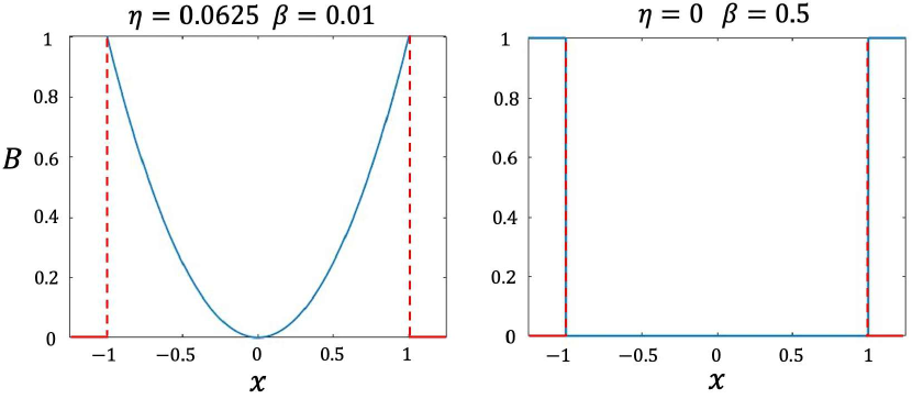
Figure 1: For a stochastic system $\mathbf{x}[k+1]=\mathbf{x}[k]+\mathbf{v}$, where $\mathbf{v}\sim\mathcal{N}(0,0.1^{2})$ is an independent additive zero-mean Gaussian noise with standard deviation $0.1$. We consider $X_{\mathrm{s}}=[-1,1]$ and $X_{0}=[-0.25,0.25]$. Two different stochastic barrier functions are shown: (right) the indicator function on the unsafe set, and (left) a 4th degree polynomial as synthesized via SoS optimization for a time horizon $H=10$.

Following Remark 2, it is clear that the key challenge in the SBF approach is in finding a valid $B$ that does not lead to excessively conservative results. Let $\mathcal{B}\subset\{f:\mathbb{R}^{n_{x}}\to\mathbb{R}_{\geq 0}\}$ be a class of non-negative functions, e.g., exponential or Sum or Square (SoS). Then, the problem of searching for a valid barrier can be formulated as the solution of the following optimization problem:

$$\max_{B\in\mathcal{B}}\;1-(\eta+\beta H)$$ (11)

subject to:

$$\qquad\qquad\inf_{x\in X_{\mathrm{u}}}B(x)\geq 1$$

$$\qquad\qquad\eta=\sup_{x\in X_{0}}B(x)$$

$$\qquad\qquad\beta=\sup_{x\in X_{\mathrm{s}}}\big{(}\mathbb{E}_{x^{\prime}\sim T(x^{\prime}\mid x,\pi(x))}[B(x^{\prime})]-B(x)\big{)}.$$

In the case, where $\mathcal{B}$ is the class of exponential or SoS functions and dynamics function $F$ is polynomial in $\mathbf{x}$ and linear in $\mathbf{v}$, the above optimization problem can be reformulated as a convex optimization problem [17, 18]. However, in the more general setting, the optimization problem in (11) is non-convex, and relaxations, which generally lead to partitioning of $X_{s}$, or ad-hoc methods are required to solve it efficiently [19, 13, 20].

Remark 3.

Note that Theorem 2 only requires $B$ to be almost surely continuous. That is, $B$ can be discontinuous in a set of (Lebesque) measure $0$. Consequently, $B$ can be taken to be a piecewise continuous functions. In practice, this can often be advantageous especially in the cases where $F$ is nonlinear [21].

3.1 Control Synthesis with SBFs

We now study how to find a policy $\pi$ that maximizes $P_{\mathrm{s}}$ using SBFs. In particular, consider a stationary policy (feedback controller) $\pi(\cdot\mid\theta):X\to U$ parameterized in some parameters $\theta\in\mathbb{R}^{n_{\theta}}$. Then, control synthesis with SBFs can be performed by modifying the optimization problem in (11) to the following:

$$\max_{B\in\mathcal{B},\theta\in\mathbb{R}^{n_{\theta}}}1-(\eta+\beta H)$$ (12)

subject to:

$$\qquad\qquad\inf_{x\in X_{\mathrm{u}}}B(x)\geq 1$$

$$\qquad\qquad\eta=\sup_{x\in X_{0}}B(x)$$

$$\qquad\qquad\beta=\sup_{x\in X_{\mathrm{s}}}\big{(}\mathbb{E}_{x^{\prime}\sim T(x^{\prime}\mid x,\pi(x\mid\theta))}[B(x^{\prime})]-B(x)\big{)}.$$

This optimization problem aims to simultaneously synthesize a barrier function $B$ and a stationary policy (feedback controller) $\pi$. Unfortunately, because the expectation in the $\beta$ term depends on both $\pi$ and $B$, the resulting optimization problem is generally non-convex [22, 23]. To address this problem, recent approaches employ iterative methods [13, 6, 8]. They generally proceed by first finding a $B$ for a fixed $\pi$ and then updating $\pi$ to maximize the lower bound on $P_{\mathrm{s}}$, i.e., $1-(\eta+\beta H)$, for the fixed $B$. By repeating this process, the lower bound on $P_{\mathrm{s}}$ is shown to improve. Additionally, approaches employing machine learning have been recently developed [24].

As discussed, there are two main sources of conservatism in bounding $P_{\mathrm{s}}$ using SBFs: (i) the choice of the barrier, and (ii) the $\beta$ term in (9), which is obtained as a uniform bound over the safe set. Both of these sources of errors can be mitigated by abstraction-based approaches, usually at the price of an increased computational effort.

4 Discrete Abstraction

Another class of well-established approaches to computing (a lower bound) for $P_{\mathrm{s}}$ and a policy $\pi$ that maximizes $P_{\mathrm{s}}$ is based on (discrete) abstraction. Intuitively, these approaches aim to numerically solve the continuous DP in (4)-(5) by discretizing $X$, while accounting for the error induced by discretization. We again start with the case where a deterministic Markov policy $\pi$ is given, and consider the control synthesis case in Section 4.2.

Abstraction-based methods first partition the safe set $X_{\mathrm{s}}$ into $n_{p}$ sets $X_{1},\ldots,X_{n_{p}}$ and treat $X_{\mathrm{u}}$ as another discrete region (i.e., $X_{n_{p}+1}=X_{\mathrm{u}}$), resulting in a total of $n_{p}+1$ regions. For $k\in\{0,...,H-1\}$ and a given policy $\pi$, one can then define piecewise-constant functions

$$\gamma^{\pi}_{k}(x)=\begin{cases}\gamma^{\pi}_{k,1}&\text{if }x\in X_{1}\\ \;\;\vdots&\quad\;\vdots\\ \gamma^{\pi}_{k,n_{p}}&\text{if }x\in X_{n_{p}}\\ \gamma^{\pi}_{k,n_{p}+1}&\text{otherwise}\end{cases}$$

recursively, for $i\in\{1,\ldots,n_{p}+1\}$, as:

$$\gamma^{\pi}_{H}(x)=\gamma^{\pi}_{H,i}:=\max_{x\in X_{i}}\mathbbm{1}(x,X_{\mathrm{u}})$$ (13)

$$\gamma^{\pi}_{k}(x)=\gamma^{\pi}_{k,i}:=\max_{x\in X_{i}}\Big{(}\mathbbm{1}(x,X_{\mathrm{u}})+$$

$$\qquad\qquad\qquad\qquad\mathbbm{1}(x,X_{\mathrm{s}})\sum_{j=1}^{n_{p}+1}\gamma^{\pi}_{k+1,j}T(X_{j}\mid x,\pi_{k}(x))\Big{)}.$$ (14)

Because of the maximum operator in (13)-(14), $\gamma^{\pi}_{k}(x)$ over-approximates $V^{\pi}_{k}(x)$, which is the probability of reaching the unsafe set starting from $x$ in the next $H-k$ time steps. This leads to the following theorem.

Theorem 3.

Let $\gamma^{\pi}_{k}$ be defined as in (13)-(14). Then, it holds that

$$P_{\mathrm{s}}(X_{\mathrm{s}},x_{0},H\mid\pi)\geq 1-\gamma^{\pi}_{0}(x_{0}).$$

Proof.

Because of Theorem 1 it is enough to show that for each $k\in\{0,...,H\}$ and $x\in X$, it holds that $V_{k}(x)\leq\gamma^{\pi}_{k}(x).$ The case $x\in X_{i}$ for $X_{i}\cap X_{\mathrm{u}}\neq\emptyset$ is trivially verified. Consequently, in what follows we assume $x\in X_{i}\subseteq X_{\mathrm{s}}$. The proof is by induction. Base case is $k=H-1$, in this case we have

$$V^{\pi}_{H-1}(x) =T(X_{\mathrm{u}}\mid x,\pi_{H-1}(x))$$

$$\leq\max_{x\in X_{i}}T(X_{\mathrm{u}}\mid x,\pi_{H-1}(x))$$

$$\leq\max_{x\in X_{i}}\sum_{j=1}^{n_{p}+1}\gamma^{\pi}_{H,j}T(X_{j}\mid x,\pi_{H-1}(x))$$

$$=\gamma^{\pi}_{H-1}(x)$$

For the induction case, assume $x\in X_{\mathrm{s}}.$ Then, under the assumption that $V^{\pi}_{k+1}(x)\leq\gamma^{\pi}_{k+1}(x)$ (induction hypothesis), it follows that:

$$V^{\pi}_{k}(x) =\mathbb{E}_{x^{\prime}\sim T(\cdot\mid x,\pi_{k}(x))}[V^{\pi}_{k+1}(x^{\prime})]$$

$$\leq\mathbb{E}_{x^{\prime}\sim T(\cdot\mid x,\pi_{k}(x))}[\gamma^{\pi}_{k+1}(x^{\prime})]$$

$$=\sum_{j=1}^{n_{p}+1}\gamma^{\pi}_{k+1,j}T(X_{j}\mid x,\pi_{k}(x))$$

$$=\gamma^{\pi}_{k}(x)$$

∎

Remark 4.

Note that if in (13)-(14), we replace the maximum operators with the minimum, then the solution of the resulting program returns a lower bound of $V^{\pi}_{0}$ and consequently an upper-bound on $P_{\mathrm{s}}$.

Since $\gamma_{0}^{\pi}$ is a piecewise-constant function and $\gamma_{0,i}^{\pi}$ is the unsafety probability bound for region $X_{i}$, (13)-(14) can be viewed as a DP for a discrete abstraction of System (1). In that view, the abstraction is a (time-inhomogenous) Markov chain (MC) $\mathcal{M}=(Q,P_{\mathcal{M}})$, where $Q=\{q_{1},\ldots,q_{n_{p}+1}\}$ is the state space such that $q_{i}$ represents region $X_{i}$, and $P_{\mathcal{M}}:Q\times Q\times\mathbb{N}_{<H}\to[0,1]$ is the transition probability function such that $P_{\mathcal{M}}(q_{i},q_{j},k)$ is the probability of transitioning from partition $X_{i}$ to $X_{j}$ at time step $k\in\mathbb{N}_{<H}$, i.e.,

$$P_{\mathcal{M}}(q_{i},q_{j},k)=\begin{cases}T(X_{j}\mid x^{*},\pi(x^{*}))&\text{if }i\neq n_{p}+1\\ 1&\text{if }i,j=n_{p}+1\\ 0&\text{otherwise,}\end{cases}$$

where $x^{*}=\arg\max_{x\in X_{i}}\sum_{j=1}^{n_{p}+1}\gamma^{\pi}_{k+1,j}T(X_{j}\mid x,\pi_{k}(x))$.

Computation of $\gamma^{\pi}_{k}$ reduces to recursively solving the following maximization problem:

$$\max_{x\in X_{i}}\sum_{j=1}^{n_{p}+1}\gamma^{\pi}_{k+1,j}T(X_{j}\mid x,\pi(x)).$$ (15)

That is, to find the input point that maximizes a linear combination of the transition probabilities for System (1). Since a positive weighted combination of convex (concave) functions is still convex (concave), (15) can be solved exactly in the case $T$ is either concave or convex in $x$. Nevertheless, in the more general case, obtaining exact solutions of this optimization problem becomes infeasible. In what follows, we consider a relaxation of (15) into a linear programming problem that leads to a well-known model, called interval Markov chains (IMC) or decision processes (IMDPs).

4.1 Abstraction to Interval Markov Processes

To relax the maximization problem in (15), we note that for each $x\in X_{i}$, $T(\cdot\mid x,\pi(x))$ is a discrete probability distribution over regions $X_{1},\ldots,X_{n_{p}},X_{\mathrm{u}}$. Consequently, (15) weighs term $\gamma^{\pi}_{k+1,j}$ with the probability of transitioning to any of the $n_{p}+1$ partitions of $X$. This observation leads to Proposition 1 below, where (15) is relaxed to a linear programming problem.

Proposition 1.

For partition $X_{i}\subseteq X_{\mathrm{s}},$ let $\bar{\gamma}^{k}_{i}$ be the solution of the following linear programming problem:

$$\bar{\gamma}^{k}_{i}=\max_{t\in[0,1]^{n_{p}+1}}\sum_{j=1}^{n_{p}+1}\gamma^{\pi}_{k+1,j}\,t_{j}$$

subject to:

$$\qquad t_{j}\in\big{[}\min_{x\in X_{i}}T(X_{j}\mid x,\pi_{k}(x)),\max_{x\in X_{i}}T(X_{j}\mid x,\pi_{k}(x))\big{]}$$

$$\qquad\sum_{j=1}^{n_{p}+1}t_{j}=1,$$

where $t_{j}$ is the j-th component of vector $t$. Then, it holds that $\bar{\gamma}^{k}_{i}\geq{\gamma}^{k}_{i}=\max_{x\in X_{i}}\sum_{j=1}^{n_{p}+1}\gamma^{\pi}_{k+1,j}T(X_{j}\mid x,\pi(x)).$

In Proposition 1, we model the likelihood of transitioning between each pair of states as intervals of probabilities, where the intervals are composed of all the valid transition probabilities for each point in the starting partition. In this view, the introduced relaxation is in fact a relaxation of the MC abstraction $\mathcal{M}$ of System (1) to an Interval MC (IMC) [25, 26] $\mathcal{I}=(Q,\check{P}_{\mathcal{I}},\hat{P}_{\mathcal{I}})$, where $Q$ is the same as in MC $\mathcal{M}$, and $\check{P}_{\mathcal{I}},\hat{P}_{\mathcal{I}}:Q\times Q\to[0,1]$ are, respectively, the lower and upper bound of the transition probability between each pair of states such that

$$\check{P}(q_{i},q_{j})=\begin{cases}\min_{x\in X_{i}}T(X_{j}\mid x,\pi_{k}(x))&\text{if }i\neq n_{p}+1\\ 1&\text{if }i,j=n_{p}+1\\ 0&\text{otherwise,}\end{cases}$$

$$\hat{P}(q_{i},q_{j})=\begin{cases}\max_{x\in X_{i}}T(X_{j}\mid x,\pi_{k}(x))&\text{if }i\neq n_{p}+1\\ 1&\text{if }i,j=n_{p}+1\\ 0&\text{otherwise.}\end{cases}$$

Consequently, it follows that, in solving the LP in Proposition 1, we select the more conservative feasible distribution w.r.t. probabilistic safety within the set of feasible distributions.

Approach	Soundness	Optimality	Accuracy	Computational Effort*	Scalability	Nonlinear Dynamics
Stochastic Barrier Function	$+$	$-$	$-$	$+$	$-$	$+$
Discrete Abstraction	$+$	$+$	$+$	$-$	$-$	$+$

Table 1: Summary of pros and cons of stochastic barrier function and discrete abstraction methods. *Computational Effort is w.r.t. the number of required optimization problems.

Remark 5.

The optimization problem in Proposition 1 can be solved particularly efficiently due to the specific structure of the linear program. In particular, as shown in [26], one can simply order states based on the value of $\gamma_{k+1}^{\pi}$ and then assign upper or lower bounds based on the ordering and on the fact that $\sum_{j=1}^{n_{p}+1}t_{j}=1.$ However, note that to solve the DP in (13)-(14), the resulting linear program problem needs to be solved $H$ times for each of the $n_{p}+1$ states in $Q$.

Remark 6.

Abstraction based methods are numerical methods. As a consequence, their precision is dependent on the discretization of the state space. An example is illustrated in Figure 2, where we show how for a finer partition, the precision of approach increases (a proof of convergence to $P_{s}$ is given in Section 4) and the resulting bound is greater than $0.8375$, the value obtained in Figure 1 for stochastic barrier functions with SoS optimization for the same setting. How to optimally discretizing the safe set, while limiting the explosion of the partition size, is still an active area of research, e.g., [3, 27].

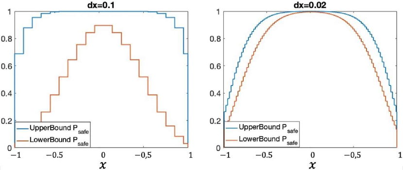
Figure 2: We consider the same setting as in Figure 1 and for each state in the safe set, we plot upper and lower bound of the probability of remaining within the safe set $[-1,1]$ for $10$ time steps starting from that state using two IMC abstractions: one obtained by discretizing the safe set uniformly with discretization step $dx=0.1$ and the other with $dx=0.02.$ For the initial set $X_{0}=[-0.25,0.25]$ we obtain a lower bound on $P_{\mathrm{s}}$ of $0.756$ for the case $dx=0.1$ and $0.975$ for $dx=0.02$.

Remark 7.

Note that an alternative approach for approximately solving (14) would be to associate a representative point $x_{i}\in X_{i}$ to each partition and then consider the following approximation

$$\max_{x\in X_{i}}\sum_{j=1}^{n_{p}+1}\gamma^{\pi}_{k+1,j}T(X_{j}\mid x,\pi_{k}(x))\approx\\ \sum_{j=1}^{n_{p}+1}\gamma^{\pi}_{k+1,j}T(X_{j}\mid x_{i},\pi_{k}(x_{i})).$$ (16)

The resulting abstraction leads to an MC with the same state space $Q$, and the transition probabilities between each pair of states are computed using representative points in the starting region as shown in (16). Similar numerical approaches have been widely studied in the literature, including also for continuous-time systems [28], and approaches to quantify the resulting error have been developed [29, 30]. However, similar to SBF (see Theorem 2), the resulting error grows linearly with time and is generally more conservative compared to abstracting to an IMC (or IMDP).

4.2 Control Synthesis with IMDPs

For control policy computation, the set of controls or actions $U$ should be included in the abstraction model. Hence, the abstraction becomes an Interval Markov Decision Process (IMDP) $\mathcal{I}=(Q,U,\check{P},\hat{P})$, where the transition probability bounds $\check{P},\hat{P}:Q\times U\times Q\to[0,1]$ are now also functions of $U$, i.e., given $q_{i},q_{j}\in Q$ and $a\in U$, $\check{P}(q_{i},a,q_{j})$ and $\hat{P}(q_{i},a,q_{j})$ are the lower- and upper-bound transition probability from $q_{i}$ to $q_{j}$ under action $a$, respectively. An optimal policy via IMDP abstractions for region $X_{i}\subseteq X_{s}$ can then be computed by solving the following value iteration, which combines Proposition 1 with (13)-(14), and where we iteratively seek for the action that minimizes the probability that $\mathbf{x}_{k}$ enters the unsafe region $X_{\mathrm{u}}$.

$$\bar{\gamma}^{*}_{H,i}=\max_{x\in X_{i}}\mathbbm{1}(x,X_{\mathrm{u}})$$ (17)

$$\bar{\gamma}^{*}_{k,i}=\min_{a\in U}\max_{t\in T^{i}_{a}}\sum_{j=1}^{n_{p}+1}\bar{\gamma}^{*}_{k+1,j}t_{j},$$ (18)

where for $i\leq n_{p}$ we define

$$T^{i}_{a}=\Big{\{}t\in[0,1]^{n_{p}+1}\mid t_{j}\in\big{[}\inf_{x\in X_{i}}T(X_{j}\mid x,a),\\ \sup_{x\in X_{i}}T(X_{j}\mid x,a)\big{]},\;\sum_{j=1}^{n_{p}+1}t_{j}=1\Big{\}}.$$

and

$$T^{n_{p}+1}_{a}=\{t\in[0,1]^{n_{p}+1}\mid t_{j}=0\text{ for $j\leq n_{p}$},\;\,t_{n_{p}+1}=1\}.$$

Note that in the inner maximization problem in (18), we seek for the feasible distribution maximizing the problem posed in Proposition 1. Consequently, synthesizing a policy according to (17)-(18) boils down to recursively solving the following min-max optimization problem for each partition $X_{i}\subseteq X_{\mathrm{s}}$

$$\min_{a\in U}\max_{t\in T^{i}_{a}}\sum_{j=1}^{n_{p}+1}\bar{\gamma}^{*}_{k+1,j}t_{j}.$$ (19)

If $U$ is discrete, then we simply need to apply Proposition 1 $|U|$ times, one for each action, and then take the action that minimizes the expression. If $U$ is uncountable, then in the case where $T$ is a convex or concave function of $a$, a solution to (19) can be found efficiently via convex optimization [31]. For the more general cases, where one cannot rely on convex optimization, a sub-optimal policy can be found via heuristics or by discretizing $U$ [12].

The following theorem guarantees that the solution of the DP in (17)-(18) returns a lower bound on probabilistic safety for System (1) and that the resulting policy converges to the optimal policy in the limit of a fine enough partition.

Theorem 4.

Let $\bar{\gamma}^{*}_{k}$ be as defined in (17)-(18). Then, for any $x\in X,$ it holds that $\bar{\gamma}^{*}_{0}(x)\geq V^{*}_{0}(x).$ Furthermore, assume that $X_{\mathrm{s}}$ is a bounded hyper-rectangle that it is discretized uniformly. Then for every $x\in X$, in the limit of $n_{p}\to\infty$, we have that $\bar{\gamma}^{*}_{0}(x)$ converges uniformly to $V^{*}_{0}(x).$

Remark 8.

Note that in the proof of Theorem 4, reported in Section 7, we characterize the convergence rate of (17)-(18) to the optimal policy and to $P_{s}$. Nevertheless, the resulting convergence rate is generally conservative and to bound the error of abstraction-based methods, a much less conservative approach is as follows. For a given policy $\pi$, possibly obtained by solving (17)-(18), solve (13)-(14), to get a lower bound of $P_{\mathrm{s}}(X_{\mathrm{s}},x,H\mid\pi)$. Then, an upper bound can be similarly obtained by solving the following DP:

$$\gamma^{\pi,L}_{H}(x)=\gamma^{\pi,L}_{H,i}:=\min_{x\in X_{i}}\mathbbm{1}(x,X_{\mathrm{u}}),$$ (20)

$$\gamma^{\pi,L}_{k}(x)=\gamma^{\pi,L}_{k,i}:=\min_{t\in T^{i}_{\pi_{k}(x)}}\sum_{j=1}^{n_{p}+1}\bar{\gamma}^{*}_{k+1,j}t_{j},$$ (21)

where $T^{i}_{\pi_{k}(x)}$ is defined as in (18). Intuitively, in the above problem we iteratively seek for the feasible distribution that minimizes the probability of reaching the unsafe region, thus $1-\gamma^{\pi,L}_{k}(x)$ returns an upper bound of $1-P_{\mathrm{s}}(X_{\mathrm{s}},x,H\mid\pi)$, as also illustrated in Figure 2.

5 Abstractions vs Barriers: Pros and Cons

Since both IMDP abstractions and SBFs are introduced under the framework of DP, we can now discuss pros and cons of the two approaches in terms of: soundness, optimality, accuracy, computational effort, and scalability.

• Soundness: As we show in Theorem 2 and 4, both approaches are guaranteed to return a valid lower bound on $P_{s}$.

• Optimality Guarantees: As the $\beta$ term in Theorem 2 is obtained by the supremum expected change for all points in $X_{\mathrm{s}},$ the policy synthesized with SBF-based approaches are necessarily sub-optimal. Similarly, there are no convergence guarantees of the safety certificate to $P_{s}.$ In contrast, for IMDP based approaches, as proved in Theorem 4, for a fine enough partition, both the policy and the certificate of safety converges to the optimal values for System (1).

• Accuracy: As illustrated in Figures 1 and 2, IMDP based approaches can generally provide less conservative bounds on $P_{\mathrm{s}}$. However, this comes at the price of a fine enough partition.

• Computational Effort: IMDP abstraction methods always require to partition the state space and to solve a DP over the resulting discretized space. Consequently, IMDP approaches necessitate to solve a number of linear programs that depends linearly on both the number of states in the partition and of the time horizon. While, as explained in Remark 5, each of these problems can be solved efficiently and they are highly parallelizible, SBF-based approaches only require to solve a single (in general non-convex) optimization process. Furthermore, in the case of linear or polynomial dynamics, the resulting optimization problem can often be solved without any partitioning by employing existing tools from convex optimization.

• Scalability: In terms of scalability w.r.t. the dimensionality of $X$, both methods generally suffer. Abstraction-based methods face the state-space explosion problem since the size of discretization grows exponentially with dimensionality. Similarly, as dimensionality grows, existing SBF methods face exponential increase in complexity. For instance, SoS-based approaches [17] experience a (exponential) blow up in the number of basis functions, e.g., number of monomials, leading to exponential growth in the optimization parameters. Alternative approaches that parameterise an SBF as a neural network [19, 24, 20] also experience exponential complexity in the dimension of $X$ to prove that a neural network is a valid SBF and to compute $\eta$ and $\beta$ as defined in Theorem 2.

A summary of the pros and cons is reported in Table 1. In this table, computational effort is w.r.t. the number of optimization problems that each method is required to solve. As explained above, this is not necessarily equivalent to time complexity of the algorithms.

From the above discussion it becomes clear how abstraction-based methods and SBFs are complementary approaches, with a trade-off between computational demands and accuracy. Consequently, the choice of the method should depend on the particular application. We should also mention that often one is interested in properties beyond safety and reachability, such as temporal logic properties. While this problem has been well studied for abstraction-based methods [10], only few works have recently considered this problem for SBFs [23].

6 Conclusion and Future Directions

Safety analysis of stochastic systems is a major problem in today’s world, of which autonomous cyber-physical systems are becoming an integral part. Existing methods that allow such analysis are either based on stochastic barrier functions or discrete abstraction. Our analysis shows that both of these methods arise as approximations of a stochastic DP problem. This view unifies these approaches and allows a fair comparison, which in turn reveals that the methods are complementary with their own strengths and weaknesses. Hence, the choice of the approach should depends on the particular application under consideration.

Our demonstration of the effectiveness of these methods in solving the safety DP problem in this work gives rise to several open research questions. The first question is rooted in the connection that this paper establishes between the SBFs and abstraction-based methods and the revealed fact that they are complementary approaches with their own pros and cons. Specifically, the open question is, given that knowledge, is it possible to devise new approaches that integrate their strengths and mitigate their weaknesses and improve scalability of existing approaches? The second question comes from the observation that only a few approaches for controller synthesis algorithms exist, and they are generally limited to discrete or convex settings [23, 31, 17]. Therefore, there is a need for more research to tackle the control synthesis problem with better and more general algorithms. Another interesting question is related to what this paper does not consider. That is, in this paper, we only consider systems with uncertainty rooted in the noise in the dynamics of the system (i.e., aleatoric uncertainty); however, often the noise characteristics or the dynamics of the system are themselves uncertain. This setting is recently attracting interest from the control and machine learning communities [32]. However, how to provide guarantees of safety and synthesize controllers for this more general setting is still an open question.

This work poses a theoretical foundation for the computation of safety guarantees for stochastic systems. By developing a common ground from which both SBFs and abstraction-based methods are developed, we hope that this work stimulates new research at the intersection of these frameworks. We believe that these methods may finally allow one to obtain safety guarantees for real-world control systems.

7 Proofs

7.1 Proof of Theorem 1

Define $P_{\mathrm{u}}(X_{\mathrm{s}},x_{0},H\mid\pi):=1-P_{\mathrm{s}}(X_{\mathrm{s}},x_{0},H\mid\pi).$ Then, to prove the result it is enough to show that

$$\inf_{\pi\in\Pi}P_{\mathrm{u}}(X_{\mathrm{s}},x_{0},H\mid\pi)=V^{*}_{0}(x_{0}).$$

In the proof we are going to require the following lemma, which, for $\pi\in\Pi$ allows us to represent $P_{\mathrm{u}}(X_{\mathrm{s}},x_{0},H\mid\pi)$ via dynamic programming for history-dependent, possibly random, policies.

Lemma 2.

For any $\pi=(\pi_{0},...,\pi_{H-1})\in\Pi,$ $k\in\{0,...,H\}$, let $\bar{V}_{k}^{\pi}:X^{k+1}\to[0,1]$ be defined as:

$$\bar{V}^{\pi}_{H}(x_{0},...,x_{H})=\mathbbm{1}(x_{H},X_{\mathrm{u}})$$

$$\bar{V}_{k}^{\pi}(x_{0},...,x_{k})=\mathbbm{1}(x_{k},X_{\mathrm{u}})+$$

$$\qquad\mathbbm{1}(x_{k},X_{\mathrm{s}})\mathbb{E}_{x^{\prime}\sim T(\cdot\mid x_{k},\pi_{k}(x_{0},...,x_{k}))}[\bar{V}^{\pi}_{k+1}(x_{0},...,x_{k},x^{\prime})].$$

Then, it holds that

$$P_{\mathrm{u}}(X_{\mathrm{s}},x_{0},H\mid\pi)=\bar{V}^{\pi}_{0}(x_{0}).$$

Proof.

The proof is by induction over the time index $k$. Define

$$P_{\mathrm{u}}^{[x_{0},...,x_{k}]}(X_{\mathrm{s}},[k,H]\mid\pi)=$$

$$\quad P[\exists k^{\prime}\in[k,H]\;s.t.\;\mathbf{x}_{k^{\prime}}\in X_{\mathrm{u}}\mid\mathbf{x}_{0}=x_{0},...,\mathbf{x}_{k}=x_{k},\pi].$$

Then, base case is for $k=H,$ that is $P_{\mathrm{u}}^{[x_{0},...,x_{H}]}(X_{\mathrm{s}},[H,H]\mid\pi)=\bar{V}_{H}(x_{0},...,x_{H}),$ which follows trivially. Then, assuming that

$$P_{\mathrm{u}}^{[x_{0},...,x_{k+1}]}(X_{\mathrm{s}},[k+1,H]\mid\pi)=\bar{V}_{k+1}^{\pi}(x_{0},...,x_{k+1}),$$

it holds that

$$P_{\mathrm{u}}^{[x_{0},...,x_{k}]}(X_{\mathrm{s}},[k,H]\mid\pi)$$

$$= P[\exists k^{\prime}\in[k,H]\;s.t.\;\mathbf{x}_{k^{\prime}}\in X_{\mathrm{u}}\mid\mathbf{x}_{0}=x_{0},...,\mathbf{x}_{k}=x_{k},\pi]$$

$$= P[\mathbf{x}_{k}\in X_{\mathrm{u}}\vee\exists k^{\prime}\in[k+1,H]\,s.t.\,\mathbf{x}_{k^{\prime}}\in X_{\mathrm{u}}$$

$$\hskip 136.5733pt\mid\mathbf{x}_{0}=x_{0},...,\mathbf{x}_{k}=x_{k},\pi]$$

$$= P[\mathbf{x}_{k}\in X_{\mathrm{u}}|\mathbf{x}_{k}=x_{k}]$$

$$+P[\exists k^{\prime}\in[k+1,H]\,s.t.\,\mathbf{x}_{k^{\prime}}\in X_{\mathrm{u}}\mid\mathbf{x}_{0}=x_{0},...,\mathbf{x}_{k}=x_{k},\pi]$$

$$-P[\mathbf{x}_{k}\in X_{\mathrm{u}}\wedge\exists k^{\prime}\in[k+1,H]\,s.t.\,\mathbf{x}_{k^{\prime}}\in X_{\mathrm{u}}$$

$$\hskip 136.5733pt\mid\mathbf{x}_{0}=x_{0},...,\mathbf{x}_{k}=x_{k},\pi]$$

$$= \mathbbm{1}(x_{k},X_{\mathrm{u}})+P[\exists k^{\prime}\in[k+1,H]\,s.t.\,\mathbf{x}_{k^{\prime}}\in X_{\mathrm{u}}$$

$$\hskip 136.5733pt\mid\mathbf{x}_{0}=x_{0},...,\mathbf{x}_{k}=x_{k},\pi]$$

$$-\mathbbm{1}(x_{k},X_{\mathrm{u}})P[\exists k^{\prime}\in[k+1,H]\,s.t.\,\mathbf{x}_{k^{\prime}}\in X_{\mathrm{u}}$$

$$\hskip 136.5733pt\mid\mathbf{x}_{0}=x_{0},...,\mathbf{x}_{k}=x_{k},\pi]$$

$$= \mathbbm{1}(x_{k},X_{\mathrm{u}})+\big{(}1-\mathbbm{1}(x_{k},X_{\mathrm{u}})\big{)}P[\exists k^{\prime}\in[k+1,H]\,s.t.\,\mathbf{x}_{k^{\prime}}\in X_{\mathrm{u}}$$

$$\hskip 136.5733pt\mid\mathbf{x}_{0}=x_{0},...,\mathbf{x}_{k}=x_{k},\pi]$$

$$= \mathbbm{1}(x_{k},X_{\mathrm{u}})+\mathbbm{1}(x_{k},X_{\mathrm{s}})P[\exists k^{\prime}\in[k+1,H]\,s.t.\,\mathbf{x}_{k^{\prime}}\in X_{\mathrm{u}}$$

$$\hskip 136.5733pt\mid\mathbf{x}_{0}=x_{0},...,\mathbf{x}_{k}=x_{k},\pi]$$

$$= \mathbbm{1}(x_{k},X_{\mathrm{u}})+\mathbbm{1}(x_{k},X_{\mathrm{s}})\int_{X}P[\exists k^{\prime}\in[k+1,H]\,s.t.\,\mathbf{x}_{k^{\prime}}\in X_{\mathrm{u}}$$

$$\quad\mid\mathbf{x}_{0}=x_{0},...,\mathbf{x}_{k}=x_{k},\mathbf{x}_{k+1}=x^{\prime},\pi]P[\mathbf{x}_{k+1}=x^{\prime}$$

$$\hskip 113.81102pt\mid\mathbf{x}_{0}=x_{0},...,\mathbf{x}_{k}=x_{k},\pi]dx^{\prime}$$

$$= \mathbbm{1}(x_{k},X_{\mathrm{u}})+\mathbbm{1}(x_{k},X_{\mathrm{s}})\int_{X}\bar{V}_{k+1}^{\pi}(x_{0},...,x_{k},x^{\prime})P[\mathbf{x}_{k+1}=x^{\prime}$$

$$\hskip 113.81102pt\mid\mathbf{x}_{0}=x_{0},...,\mathbf{x}_{k}=x_{k},\pi]dx^{\prime}$$

$$= \bar{V}^{\pi}_{k}(x_{0},...,x_{k})$$

∎

We can now prove the main statement. As $\Pi^{M,D}\subset\Pi$, it holds that

$$\inf_{\pi\in\Pi}P_{\mathrm{u}}(X_{\mathrm{s}},X_{0},H\mid\pi)\leq\inf_{\pi\in\Pi^{M,D}}P_{\mathrm{u}}(X_{\mathrm{s}},X_{0},H\mid\pi).$$

Consequently, the proof is concluded if we can show that also holds that $\inf_{\pi\in\Pi}P_{\mathrm{u}}(X_{\mathrm{s}},X_{0},H\mid\pi)\geq\inf_{\pi\in\Pi^{M,D}}P_{\mathrm{u}}(X_{\mathrm{s}},X_{0},H\mid\pi).$ This can be done by induction over the time index $k\in\{0,H\}$. The base case is $k=H$, which follows trivially as $\forall x_{0}\in X$ it holds that for any $\pi\in\Pi,$

$$\bar{V}_{H}^{\pi}(x_{0},...,x_{H})={V}_{H}^{*}(x_{H})=\mathbbm{1}(x_{H},X_{\mathrm{u}}),$$

which is independent of the action and of the previous states. Now assume that $\forall(x_{0},...,x_{k+1})\in X^{k+1},\inf_{\pi\in\Pi}V^{\pi}_{k+1}(x_{0},...,x_{k+1})\geq V^{*}_{k+1}(x_{k+1})$, then it holds that

$$\inf_{\pi\in\Pi}\bar{V}_{k}^{\pi}(x_{0},...,x_{k})$$

$$=\inf_{\pi\in\Pi}\mathbbm{1}(x_{k},X_{\mathrm{u}})+$$

$$\qquad\quad\mathbbm{1}(x_{k},X_{\mathrm{s}})\mathbb{E}_{x^{\prime}\sim T(\cdot\mid x_{k},\pi_{k}(x_{0},...,x_{k}))}[\bar{V}^{\pi}_{k+1}(x_{0},...,x_{k},x^{\prime})]$$

$$\geq\mathbbm{1}(x_{k},X_{\mathrm{u}})+$$

$$\qquad\qquad\quad\;\;\mathbbm{1}(x_{k},X_{\mathrm{s}})\inf_{\pi\in\Pi}\mathbb{E}_{x^{\prime}\sim T(\cdot\mid x_{k},\pi_{k}(x_{0},...,x_{k}))}[{V}^{*}_{k+1}(x^{\prime})]$$

$$=\mathbbm{1}(x_{k},X_{\mathrm{u}})+\mathbbm{1}(x_{k},X_{\mathrm{s}})\inf_{a\in U}\mathbb{E}_{x^{\prime}\sim T(\cdot\mid x_{k},a)}[V^{*}_{k+1}(x^{\prime})]$$

$$=V^{*}_{k}(x_{k})$$

7.2 Proof of Theorem 4

We recall that $\bar{\gamma}^{*}_{k}$ is the solution of the following dynamic programming problem

$$\bar{\gamma}^{*}_{H}(x)=\bar{\gamma}^{*}_{H,i}:=\max_{x\in X_{i}}\mathbbm{1}(x,X_{\mathrm{u}})$$

$$\bar{\gamma}^{*}_{k}(x)=\bar{\gamma}^{*}_{k,i}:=\min_{a\in U}\max_{t\in T^{i}_{a}}\Big{(}\mathbbm{1}(x,X_{\mathrm{u}})+$$

$$\hskip 142.26378pt\mathbbm{1}(x,X_{\mathrm{s}})\sum_{j=1}^{n_{p}+1}\bar{\gamma}^{*}_{k+1,j}t_{j}\Big{)},$$

where for $i\leq n_{p}$

$$T^{i}_{a}=\Big{\{}t\in[0,1]^{n_{p}+1}\mid t_{j}\in\big{[}\inf_{x\in X_{i}}T(X_{j}\mid x,a),\\ \sup_{x\in X_{i}}T(X_{j}\mid x,a)\big{]},\;\sum_{j=1}^{n_{p}+1}t_{j}=1\Big{\}}$$

and for $i=n_{p}+1$ we have $T^{n_{p}+1}_{a}=\{t\in[0,1]^{n_{p}+1}\mid t_{j}=0\text{ for $j\leq n_{p}$}\,\wedge\,t_{n_{p}+1}=1\}.$ Then, we first have to show that for any $k\in\{0,...,H\}$ and $x\in X$ in holds that $\bar{\gamma}^{*}_{0}(x)\geq V^{*}_{0}(x).$ This can be easily proved by contradiction. In fact, assume that this statement is not true, then there must exist a strategy $\pi$ such that for $x\in X$ and $k\in\{0,...,H\}$ it holds that $\bar{\gamma}^{\pi}_{k}(x)\leq V^{\pi}_{k}(x).$ However, this contradicts Theorem 3 and Proposition 1, thus concluding the proof that $\bar{\gamma}^{*}_{0}(x)\geq V^{*}_{0}(x).$ A consequence of this result is that for any $\bar{x}\in X_{i}$, if we consider $a^{*}\in\operatorname*{arg\,min}_{a\in U}\mathbb{E}_{x^{\prime}\sim T(\cdot\mid\bar{x},a)}[V^{*}_{k+1}(x^{\prime})],$ it holds that

$$0\leq\min_{a\in U}\max_{x\in X_{i}}\mathbb{E}_{x^{\prime}\sim T(\cdot\mid x,a)}[\bar{\gamma}^{*}_{k+1}(x^{\prime})]-\mathbb{E}_{x^{\prime}\sim T(\cdot\mid\bar{x},a^{*})}[V^{*}_{k+1}(x^{\prime})]$$

$$\leq\max_{x\in X_{i}}\mathbb{E}_{x^{\prime}\sim T(\cdot\mid x,a^{*})}[\bar{\gamma}^{*}_{k+1}(x^{\prime})]-\mathbb{E}_{x^{\prime}\sim T(\cdot\mid\bar{x},a^{*})}[V^{*}_{k+1}(x^{\prime})].$$

We will use this result to prove that for any $\epsilon>0$ there exists a partition of $X$ in $n_{p}+1$ regions such that $\forall x\in X,\,\bar{\gamma}^{*}_{0}(x)-V^{*}_{0}(x)\leq\epsilon.$ That, is $\bar{\gamma}^{*}_{0}(x)$ converges uniformly to $V^{*}_{0}(x)$, thus concluding the proof.

Without any lost of generality assume that $X_{\mathrm{s}}$ is uniformly partitioned in $n_{p}$ hyper-cubes with edge of size $\delta$. Further, consider an additional set in the partition $X_{n_{p}+1}=X_{\mathrm{u}}.$ Then, the proof is as follows. We first show that for any $\bar{\epsilon}>0$ such that $\max_{x\in X}\big{(}\bar{\gamma}^{*}_{k+1}(x)-V_{k+1}^{*}(x)\big{)}\leq\bar{\epsilon}$, then for all $x\in X$ it holds that $\bar{\gamma}^{*}_{k}(x)-V_{k}^{*}(x)\leq\bar{\epsilon}+L\delta,$ where $L$ is such that for any $x,x^{\prime}\in X_{s}$ and $X_{j}\subseteq X$

$$L|x-x^{\prime}|_{\infty}\geq\max_{a\in U}|T(X_{j}\mid x,a)-T(X_{j}\mid x^{\prime},a)|,$$

which is guaranteed to exist because of the Lipschitz continuity of $T(X_{j}\mid x,a^{*})$ wrt $x$. Then, we derive a bound for $\bar{\epsilon}$ by considering the case $k=H-1$. We start with the first part of the proof.

As mentioned, we start by assuming that $\forall x\in X,\bar{\gamma}^{*}_{k+1}(x)-V_{k+1}^{*}(x)\leq\bar{\epsilon}$. Under this assumption, for $x\in X_{i}$ with $i\leq n_{p}$ select $a^{*}\in\operatorname*{arg\,min}_{a\in U}\mathbb{E}_{x^{\prime}\sim t(x^{\prime}\mid x,a)}[V^{*}_{k+1}(x^{\prime})],$ then the following holds

$$\bar{\gamma}^{*}_{k}(x) -V_{k}^{*}(x)$$

$$\leq \max_{t\in T^{i}_{a^{*}}}\sum_{j=1}^{n_{p}+1}\bar{\gamma}^{*}_{k+1,j}t_{j}-\mathbb{E}_{x^{\prime}\sim T(\cdot\mid\bar{x},a^{*})}[V^{*}_{k+1}(x^{\prime})]$$

$$\leq \max_{t\in T^{i}_{a^{*}}}\sum_{j=1}^{n_{p}+1}\bar{\gamma}^{*}_{k+1,j}t_{j}-\sum_{j=1}^{n_{p}+1}\min_{x^{\prime}\in X_{j}}V_{k+1}^{*}(x^{\prime})T(X_{j}\mid x,a^{*})$$

$$\leq \max_{t\in T^{i}_{a^{*}}}\sum_{j=1}^{n_{p}+1}\big{(}\min_{x^{\prime}\in X_{j}}V_{k+1}^{*}(x^{\prime})+\bar{\epsilon}\big{)}t_{j}-$$

$$\hskip 85.35826pt\sum_{j=1}^{n_{p}+1}\min_{x^{\prime}\in X_{j}}V_{k+1}^{*}(x^{\prime})T(X_{j}\mid x,a^{*})$$

$$\leq \bar{\epsilon}+\max_{t\in T^{i}_{a^{*}}}\sum_{j=1}^{n_{p}+1}\min_{x^{\prime}\in X_{j}}V_{k+1}^{*}(x^{\prime})\big{(}t_{j}-T(X_{j}\mid x,a^{*})\big{)}$$

$$\leq \bar{\epsilon}+\max_{t\in T^{i}_{a^{*}}}\max_{j\in\{1,...,n_{p}+1\}}\big{|}t_{j}-T(X_{j}\mid x,a^{*})\big{|}$$

$$\leq \bar{\epsilon}+L\delta,$$

where last two inequalities hold because $\sum_{j=1}^{n_{p}+1}\min_{x^{\prime}\in X_{j}}V_{k+1}^{*}(x^{\prime})\leq\min_{x^{\prime}\in X_{j}}\sum_{j=1}^{n_{p}+1}V_{k+1}^{*}(x^{\prime})\leq 1$ and becasue $t$ is a feasible distribution satisfying the constraints of Proposition 1. Note that the case $x\in X_{n_{p}+1}=X_{u}$ follows trivially as in that case $\bar{\gamma}^{*}_{k}(x)=\mathbbm{1}(x,X_{u})=V_{k}^{*}(x).$ What is left to do in order to complete the proof is to obtain a bound of $\bar{\epsilon}$ as a function of $\delta.$ We can do that by noticing that

$$\bar{\gamma}^{*}_{H-1}(x)-V_{H-1}^{*}(x)=\\ \max_{t\in T^{i}_{a^{*}}}\big{(}t_{n_{p}+1}-T(X_{\mathrm{u}}\mid x,a^{*})\big{)}\leq L\delta.$$

Consequently, to guarantee an error smaller than $\epsilon>0$, we can take $\delta\leq\frac{\epsilon}{HL},$ which results in $n_{p}\geq\big{(}\frac{lHL}{\epsilon}\big{)}^{n}+1,$ where $l=\max_{x,x^{\prime}\in X_{s}}|x-x^{\prime}|_{\infty}$.

Luca Laurenti is an assistant professor at the Delft Center for Systems and Control at TU Delft and co-director of the HERALD Delft AI Lab . He received his PhD from the Department of Computer Science, University of Oxford (UK), where he was a member of the Trinity College. Luca has a background in stochastic systems, control theory, formal methods, and artificial intelligence. His research work focuses on developing data-driven systems provably robust to interactions with a dynamic and uncertain world.

Morteza Lahijanian (Member, IEEE) is an assistant professor in the Aerospace Engineering Sciences department, an affiliated faculty at the Computer Science department, and the director of the Assured, Reliable, and Interactive Autonomous (ARIA) Systems group at the University of Colorado Boulder. He received a B.S. in Bioengineering at the University of California, Berkeley and a PhD in Mechanical Engineering at Boston University. He served as a postdoctoral scholar in Computer Science at Rice University. Prior to joining CU Boulder, he was a research scientist in the department of Computer Science at the University of Oxford. His awards include Ella Mae Lawrence R. Quarles Physical Science Achievement Award, Jack White Engineering Physics Award, and NSF GK-12 Fellowship. Dr. Lahijanian’s research interests span the areas of control theory, stochastic hybrid systems, formal methods, machine learning, and game theory with applications in robotics, particularly, motion planning, strategy synthesis, model checking, and human-robot interaction.

References

- [1] W. Schwarting, J. Alonso-Mora, and D. Rus, “Planning and decision-making for autonomous vehicles,” Annual Review of Control, Robotics, and Autonomous Systems, vol. 1, pp. 187–210, 2018.
- [2] P. E. Dupont, B. J. Nelson, M. Goldfarb, B. Hannaford, A. Menciassi, M. K. O’Malley, N. Simaan, P. Valdastri, and G.-Z. Yang, “A decade retrospective of medical robotics research from 2010 to 2020,” Science robotics, vol. 6, no. 60, p. eabi8017, 2021.
- [3] S. Adams, M. Lahijanian, and L. Laurenti, “Formal control synthesis for stochastic neural network dynamic models,” IEEE Control Systems Letters, vol. 6, pp. 2858–2863, 2022.
- [4] A. Clark, “Control barrier functions for stochastic systems,” Automatica, vol. 130, p. 109688, 2021.
- [5] H. J. Kushner, “Stochastic stability and control,” Brown Univ Providence RI, Tech. Rep., 1967.
- [6] S. Prajna, A. Jadbabaie, and G. J. Pappas, “A framework for worst-case and stochastic safety verification using barrier certificates,” IEEE Transactions on Automatic Control, vol. 52, no. 8, pp. 1415–1428, 2007.
- [7] H. J. Kushner and D. S. Clark, Stochastic approximation methods for constrained and unconstrained systems. Springer Science & Business Media, 2012, vol. 26.
- [8] A. Lavaei, S. Soudjani, A. Abate, and M. Zamani, “Automated verification and synthesis of stochastic hybrid systems: A survey,” Automatica, vol. 146, p. 110617, 2022.
- [9] M. Lahijanian, S. B. Andersson, and C. Belta, “Approximate Markovian abstractions for linear stochastic systems,” in Proceedings of the IEEE Conference on Decision and Control. Maui, HI, USA: IEEE, Dec 2012, pp. 5966–5971.
- [10] ——, “Formal verification and synthesis for discrete-time stochastic systems,” IEEE Transactions on Automatic Control, vol. 60, no. 8, pp. 2031–2045, 2015.
- [11] N. Cauchi, L. Laurenti, M. Lahijanian, A. Abate, M. Kwiatkowska, and L. Cardelli, “Efficiency through uncertainty: Scalable formal synthesis for stochastic hybrid systems,” in Proceedings of the 2019 22nd ACM International Conference on Hybrid Systems: Computation and Control. Montreal, QC, Canada: ACM, Apr. 2019.
- [12] M. Dutreix, J. Huh, and S. Coogan, “Abstraction-based synthesis for stochastic systems with omega-regular objectives,” Nonlinear Analysis: Hybrid Systems, vol. 45, p. 101204, 2022.
- [13] R. Mazouz, K. Muvvala, A. Ratheesh Babu, L. Laurenti, and M. Lahijanian, “Safety guarantees for neural network dynamic systems via stochastic barrier functions,” in Advances in Neural Information Processing Systems, 2022, pp. 9672–9686.
- [14] D. Bertsekas and S. E. Shreve, Stochastic optimal control: the discrete-time case. Athena Scientific, 1996, vol. 5.
- [15] A. Abate, M. Prandini, J. Lygeros, and S. Sastry, “Probabilistic reachability and safety for controlled discrete time stochastic hybrid systems,” Automatica, vol. 44, no. 11, pp. 2724–2734, 2008.
- [16] A. D. Ames, X. Xu, J. W. Grizzle, and P. Tabuada, “Control barrier function based quadratic programs for safety critical systems,” IEEE Transactions on Automatic Control, vol. 62, no. 8, pp. 3861–3876, 2016.
- [17] C. Santoyo, M. Dutreix, and S. Coogan, “A barrier function approach to finite-time stochastic system verification and control,” Automatica, vol. 125, p. 109439, 2021.
- [18] J. Steinhardt and R. Tedrake, “Finite-time regional verification of stochastic non-linear systems,” The International Journal of Robotics Research, vol. 31, no. 7, pp. 901–923, 2012.
- [19] F. B. Mathiesen, S. C. Calvert, and L. Laurenti, “Safety certification for stochastic systems via neural barrier functions,” IEEE Control Systems Letters, vol. 7, pp. 973–978, 2022.
- [20] A. Abate, M. Giacobbe, and D. Roy, “Learning probabilistic termination proofs,” in Computer Aided Verification: 33rd International Conference, CAV 2021, Virtual Event, July 20–23, 2021, Proceedings, Part II 33. Springer, 2021, pp. 3–26.
- [21] F. B. Mathiesen, L. Romao, S. C. Calvert, A. Abate, and L. Laurenti, “Inner approximations of stochastic programs for data-driven stochastic barrier function design,” arXiv preprint arXiv:2304.04505, 2023.
- [22] A. Agrawal and K. Sreenath, “Discrete control barrier functions for safety-critical control of discrete systems with application to bipedal robot navigation.” in Robotics: Science and Systems, vol. 13. Cambridge, MA, USA, 2017, pp. 1–10.
- [23] P. Jagtap, S. Soudjani, and M. Zamani, “Formal synthesis of stochastic systems via control barrier certificates,” IEEE Transactions on Automatic Control, vol. 66, no. 7, pp. 3097–3110, 2020.
- [24] D. Vzikelic, M. Lechner, T. A. Henzinger, and K. Chatterjee, “Learning control policies for stochastic systems with reach-avoid guarantees,” in Proceedings of the AAAI Conference on Artificial Intelligence, vol. 37, no. 10, 2023, pp. 11 926–11 935.
- [25] A. Nilim and L. El Ghaoui, “Robust control of markov decision processes with uncertain transition matrices,” Operations Research, vol. 53, no. 5, pp. 780–798, 2005.
- [26] R. Givan, S. Leach, and T. Dean, “Bounded-parameter Markov decision processes,” Artificial Intelligence, vol. 122, no. 1-2, pp. 71–109, 2000.
- [27] M. Dutreix and S. Coogan, “Efficient verification for stochastic mixed monotone systems,” in 2018 ACM/IEEE 9th International Conference on Cyber-Physical Systems (ICCPS). IEEE, 2018, pp. 150–161.
- [28] H. J. K. Kushner, H. J. Kushner, P. G. Dupuis, and P. Dupuis, Numerical methods for stochastic control problems in continuous time. Springer Science & Business Media, 2001, vol. 24.
- [29] A. Abate, J.-P. Katoen, J. Lygeros, and M. Prandini, “Approximate model checking of stochastic hybrid systems,” European Journal of Control, vol. 16, no. 6, pp. 624–641, 2010.
- [30] Z. Esmaeil, S. Soudjani, C. Gevaerts, and A. Abate, “Faust 2: Formal abstractions of uncountable-state stochastic processes,” in 21st International Conference on Tools and Algorithms for the Construction and Analysis of Systems (TACAS 2015). Newcastle University, 2015.
- [31] G. Delimpaltadakis, M. Lahijanian, M. Mazo Jr, and L. Laurenti, “Interval markov decision processes with continuous action-spaces,” HSCC, 2023.
- [32] I. Gracia, D. Boskos, L. Laurenti, and M. Mazo Jr, “Distributionally robust strategy synthesis for switched stochastic systems,” in Proceedings of the 26th ACM International Conference on Hybrid Systems: Computation and Control, 2023, pp. 1–10.