A Bayesian approach to estimate the completeness of death registration

Abstract

Civil registration and vital statistics (CRVS) systems should be the primary source of mortality data for governments. Accurate and timely measurement of the completeness of death registration helps inform interventions to improve CRVS systems and to generate reliable mortality indicators. In this work we propose the use of hierarchical Bayesian linear mixed models with Global-Local (GL) priors to estimate the completeness of death registration at global, national and subnational levels. The use of GL priors in this paper is motivated for situations where demographic covariates can explain much of the observed completeness but where unexplained within-country (i.e. by year) and between-country variability also play an important role. The use of our approach can allow institutions improve model parameter estimates and more accurately predict completeness of death registration. Our models are based on a dataset which uses Global Burden of Disease (GBD) death estimates based on the GBD 2019 and comprises 120 countries and 2,748 country-years from 1970-2019 (Demographics Collaborators, 2020). To illustrate the effectiveness of our proposal we consider the completeness of death registration in the departments of Colombia in 2017.

Keywords: Completeness of death registration, Unit-Level models, Global-Local priors, Mortality, Vital statistics, Data quality.

1. Introduction

The primary source of mortality data for national governments should be a complete civil registration and vital statistics (CRVS) (Mikkelsen et al., 2015). However, only 59% of all deaths that occur globally are estimated to be registered, with almost all unregistered deaths occurring in low- and middle-income countries (Dicker et al., 2018), hence this severely limits the utility of this data source to provide evidence on mortality trends to inform government policymaking. Reliable measurement of the completeness of death registration – that is, the percentage of deaths that are registered – is important firstly to measure the extent of under-registration of deaths and to inform interventions that aim to attain complete registration. The completeness of registration can also be used to adjust data from a death registration system and, together with model life tables, produce estimates of key mortality indicators.

Various methods to estimate completeness of death registration have been developed over several decades. A group of demographic methods named death distribution methods (DDMs) estimate completeness at ages five years and above by assessing the internal consistency of the age pattern of population and registered deaths, and make assumptions of population dynamics (Brass et al., 1975; Preston et al., 1980; Bennett and Horiuchi, 1984; Hill, 1987; Adair and Lopez, 2018; Dorrington, 2013a, b, c). DDMs either measure completeness of death registration assuming a stable population (i.e., a constant population growth rate and no migration) and using population data from a specific point in time, or assuming a closed population (i.e., no migration) and using population from two censuses to enable measurement of completeness of inter-censal death registration. The most reliable DDM has been identified as a hybrid approach using the Generalised Growth Balance and Bennett-Horiuchi methods to estimate inter-censal death registration, together with the use of age trims to minimize the impact of the assumption of no migration (Murray et al., 2010) on the accuracy of completeness. However, DDMs have several limitations, including inaccuracy of estimates and limited applicability at the subnational level because of the incompatibility of the restrictive assumptions to contemporary population dynamics, and the lack of timeliness of estimates where they are made for the period between the most recent two censuses (Adair and Lopez, 2018). Another set of methods to estimate completeness are capture-recapture methods, which involved linking of death registration data with another independent data source (Rao and Kelly, 2017). However, limitations of these methods are the availability of another independent data source, and the time required to link data sources where data quality is suboptimal. A more straightforward means of calculating completeness is to divide the number of registered deaths by the number of deaths in the population estimated by either the Global Burden of Disease (GBD) Study or United Nations (UN) World Population Prospects (Wang et al., 2020). However, with the exception of very few countries where the GBD estimates deaths for subnational populations, these estimates are only available nationally.

More recently, the empirical completeness method has been proposed to estimate completeness of death registration (Adair and Lopez, 2018). The method, which was developed from an extensive database of 110 countries from 1970 to 2015 reported in the Global Burden of Disease 2015 database, models completeness based on the key drivers of a population’s crude death rate (the number of deaths per 1,000 population). The empirical completeness method, compared with DDMs, uses only relatively limited data (and which are readily available at subnational levels), provides completeness estimates for the most recent year of death registration data, and is not reliant on assumptions about population dynamics such as closed migration that adversely affect subnational estimates. A limitation of the method, however, is that it is less reliable where the level of adult mortality is relatively high given the level of under-five mortality, such as where HIV/AIDS mortality is high or there has been a mortality shock such as a natural disaster. The method has been applied in several settings, including to estimate excess mortality from COVID-19 in Peru, to calculate subnational completeness for Indian states and 2,844 Chinese counties, to monitor completeness of community death reporting systems in Bangladesh, and to estimate cause-specific mortality rates to track attainment of Sustainable Development Goals in Myanmar (Zeng et al., 2020; Sempé et al., 2021; Adair et al., 2021; Basu and Adair, 2021; Shawon et al., 2021).

The probabilistic empirical method proposed by (Adair and Lopez, 2018) considers two linear mixed models with random effects at the country level. The covariates in the model of (Adair and Lopez, 2018) include information typically available from multiple sources, e.g., surveys, censuses and administrative records. Specifically, the first model includes predictors with information about the registered crude death rate, fraction of the population aged 65 years and over, under-five mortality rate and calendar year of death, while the second model also includes also covariate of the completeness of registration for children ages less than five years. (Adair and Lopez, 2018) also consider models for males and females to allow predictions of completeness in each case.

The modeling of demographic components using Bayesian methods is a growing and active research area with important recent advances, for example in population projections (Raftery et al., 2014; Wheldon et al., 2016), international migration flows (Azose and Raftery, 2015), projections of life expectancy (Godwin and Raftery, 2017) and estimation of maternal mortality (Alkema et al., 2017). Although the use of new Bayesian methods for demographic indicators is extensive, there have not been any attempts to use these models to estimate the completeness of death registration. Therefore, this paper adapts the empirical completeness method (Adair and Lopez, 2018) to a Bayesian framework, using first a common prior for the scale of the errors and random effects respectively and extending this to a more flexible Bayesian modeling that considers Global-Local priors (GL) for the scales of the errors and random effects respectively. The use of GL priors in this paper is motivated for situations where demographic covariates can explain much of the observed completeness but where unexplained within-country (i.e. by year) and between-country variability also play an important role.

The new models are based on a dataset updated to 2019, which uses GBD death estimates based on the GBD 2019 and now comprises 120 countries and 2,748 country-years from 1970-2019 (Demographics Collaborators, 2020). The dataset calculates observed completeness for a country-year as the number of registered deaths divided by the GBD’s estimate of total deaths. The GBD estimates total deaths by estimating under-five mortality and adult mortality rates and then using model life tables to develop complete life tables; further detail of their methods can be found in GBD 2019 Demographics Collaborators (2020). Consistent with Adair and Lopez (2018), some country-years were excluded from the database because they either experienced mortality shocks (e.g. natural disaster, conflict) or high adult mortality compared with child mortality due to, for example, HIV/AIDS or alcohol (e.g. sub-Saharan Africa, Russia in the 1990s). In such countries, the under-five mortality rate is not a reliable proxy for mortality level because of the high level of adult mortality.

To assess the performance of the proposed models to national and subnational levels we consider the completeness of death registration for the country of Colombia and its 33 departments in 2017 for both sexes, males and females based on a question in the Colombian Population Census 2018 (DANE, 2018) that asks if households experienced a death during the calendar year 2017 and whether that death was registered with the civil registration system. This comparator dataset is not included in GBD 2019 data used to develop the models.

We found the Census data can be regarded as a reliable independent estimate of completeness in departments because its estimate of national completeness of 90% (i.e. the % of reported household deaths that were reported as being registered with the civil registration system) is close to the completeness of 85% calculated by using vital registration data as the numerator and UN estimated deaths for Colombia as the denominator (UN, 2019). Also, an estimated 90% of deaths in 2017 in Colombia were reported in the Census (UN, 2019).

This paper is organized as follows. Section 2 introduces the methodology implemented in this work. Next, we introduce GL priors for the scales of the random effects and errors respectively in hierarchical linear mixed models and study their theoretical properties to allow small and large random effects when it is required. Section 3 contains the Markov chain Monte Carlo (MCMC) schemes for posterior inference of the parameters and the prior elicitation. In Section 4 we implement our proposal to estimate the completeness of the death registration at the global level and consider a prior sensitivity study. The application of the models to national and subnational levels in Colombia are given in Section 5. Finally, the concluding remarks and discussion are presented in Section 6.

2. Methodology

2.1. Linear mixed models with Global-Local priors for random effects and errors

Consider the proposed model

$$y_{ij} =\theta_{ij}+\epsilon_{ij}, j =1,...,n_{i},$$

(2.1) $$\theta_{ij} =\bm{x}_{ij}^{\textsf{T}}\bm{\beta}+u_{i}, i =1,...,m,$$

where $n_{i}>p=\dim(\bm{x}_{ij})$ and the errors $\epsilon_{ij}$ and random effects $u_{i}$ are independent and normally distributed and $\epsilon_{ij}\overset{\mathrm{ind}}{\sim}\text{Normal}(\epsilon_{ij};0,1/(\lambda_{i}\tau))$ and $u_{i}\overset{\mathrm{iid}}{\sim}\text{Normal}(u_{i};0,1/(\omega_{i}\phi))$ and where $\lambda_{i}$ and $\omega_{i}$ denote the Local scales and $\tau$ and $\phi$ denote the Global scales for the errors and random effects, respectively. In this work $y_{ij}=\log(c_{ij}/(1-c_{ij}))$ denote the logit of the completeness of registration at all ages for country $i$ and year $j$. GL priors where originally proposed by Carvalho et al. (2010) and Polson and Scott (2012). These priors have been implemented in an important number of proposals for variable selection, estimation and model selection (e.g., Armagan et al. (2013); Ghosh et al. (2016); Tang et al. (2018b); Bhattacharya et al. (2015); Bhadra et al. (2017); Bai and Ghosh (2018); Tang et al. (2018a). The global parameter in model (2.1) controls the total shrinkage of the random effects (posterior mean) towards zero (country-mean) and the local parameter allows random effects (posterior mean) to avoid this shrinkage. In the context of model (2.1) the local priors produces a conditional posterior distribution for the random effects (posterior mean) with a peak at zero to shrink small random effects (posterior mean) and heavy tails to avoid this shrinkage when required. In this work we consider, for the first time to the best of our knowledge, the use of GL priors for the random effects and errors in the linear mixed model given by (2.1). As we will discuss, the use of GL priors is motivated for the applied site where demographic covariates can explain the completeness of death registration well but variability of the data at the country and country-year levels play an important role. The list of shrinkage priors in the literature is extensive. To evaluate the performance of different GL priors in model (2.1) to estimate the completeness of death registration we use local shrinkage behaviors with different shrinkage behaviors around the origin and tails. Specifically, we consider the Horseshoe (Carvalho et al., 2010), Laplace (Frühwirth-Schnatter and Wagner, 2011; Brown and Griffin, 2010) and local Student-t (Griffin and Brown, 2005) priors for $\omega_{i}$. The priors are illustrated in Table 1 where HS and Half-Cauchy priors belong to the family of polynomial heavy tailed priors while the LA priors correspond to the family of exponential heavy tailed priors. We also consider the local Student-t prior with a weakly informative prior for the degrees of freedom we present in Section 3. Although both the HS and local Student-t priors produce a conditional distributions for the random effects with polynomial tails, the conditional distribution under the HS is more peaked around zero than the conditional distribution obtained with the local Student-t prior. As a result, more shrinkage towards zero for small random effects is produced under the HS than under the local Student-t. For the local scale of the errors $\lambda_{i}$ we consider the Half-Cauchy prior proposed by Polson and Scott (2012) for top-levels scale parameters in Bayesian hierarchical models.

Name	$\pi_{\omega}(x)$	Reference	Tail
Laplace	$x^{-2}\exp(-1/x)$	Frühwirth-Schnatter and Wagner (2011); Brown and Griffin (2010)	Exponential
Horseshoe	$x^{-1/2}(1+x)^{-1}$	Carvalho et al. (2010)	Polynomial
Local Student-t	$x^{\nu/2-1}\exp(-x\nu/2)$	Griffin and Brown (2005)	Polynomial
	$\pi_{\lambda}(x)$	Reference
Half-Cauchy	$(1+x)^{-2}$	Polson and Scott (2012)	Polynomial

Table 1. Priors distributions $\pi_{\omega}(x)$ and $\pi_{\lambda}(x)$ for the local scales of the random effects and errors respectively. Tails refer to the tail behavior of the marginal distribution for $u_{i}$ and $\bm{\theta}_{i}$.

We assume non-informative Gamma priors for each of the global scales, $\tau$ and $\phi$. To compare the performance of our proposal we also consider non-informative Gamma priors under the assumption of a common scale $\zeta_{\epsilon}$ for the errors, $\epsilon_{ij}\overset{\mathrm{ind}}{\sim}\text{Normal}(\epsilon_{ij};0,1/\zeta_{\epsilon})$. In addition, in order to compare the frequentist version of model (2.1) we also consider a common scale $\zeta_{u}$ for the random effects, $u_{i}\overset{\mathrm{iid}}{\sim}\text{Normal}(u_{i};0,1/\zeta_{u})$, and a common scale $\zeta_{\epsilon}$ for the errors, respectively. We consider the same covariates given in Adair and Lopez (2018) in our proposed Bayesian models given in (2.1) to estimate the completeness of death registration for both sexes (males and females) as follow

Model 1: $$\;\;\;x_{ij}=(1,\text{RegCDR}_{ij},\text{RegCDR}_{ij}^{2},\%65_{ij}^{2},\text{ln(5q0)}_{ij},\text{C5q0}_{ij},\text{year}_{ij}),$$

(2.2) Model 2: $$\;\;\;x_{ij}=(1,\text{RegCDR}_{ij},\text{RegCDR}_{ij}^{2},\%65_{ij}^{2},\text{ln(5q0)}_{ij},\text{year}_{ij}),$$

where RegCDR is the registered crude death rate (registered deaths divided by population multiplied by 1000), RegCDR² is the registered crude death rate squared, %65 is the fraction of the population aged 65 years and over, ln(5q0) is the natural log of the estimate of the true under-five mortality rate, C5q0 is the is the completeness of registered under-five deaths (estimated as the under-five mortality rate from registration data divided by the estimate of the true under-five mortality rate), and year is calendar year of death. As is pointed out by Adair and Lopez (2018), the under-five mortality rate and the population aged 65 years and over are important drivers of the registered crude death rates in populations. We also consider in (2.1) models for males and females independently with the same predictors but sharing the same information for C5q0 which are likely to be similar for males and females as is pointed out by Wang et al. (2014) and successfully implemented in Adair and Lopez (2018).

The joint prior distribution for the parameters $\bm{\beta}$, $\bm{\omega}=(\omega_{1},...,\omega_{m})^{\textsf{T}}$, $\bm{\lambda}=(\lambda_{1},...,\lambda_{m})^{\textsf{T}}$, $\tau$ and $\phi$ is given as follows:

(2.3) $$\pi(\bm{\beta},\bm{\lambda},\tau,\bm{\omega},\phi)\propto\pi(\phi)\pi(\tau)\prod_{i=1}^{m}\pi(\omega_{i})\pi(\lambda_{i}),$$

where the conditional posterior mean of the random effects $u_{i}$ is given by

(2.4) $$E(u_{i}|\bm{\beta},\bm{\lambda},\tau,\bm{\omega},\phi,\bm{y}_{i})=\gamma_{i}(\bar{\bm{y}}_{i}-\bar{\bm{x}}_{i}^{\textsf{T}}\bm{\beta}_{i}),$$

and $\gamma_{i}=(\lambda_{i}\tau)/(\lambda_{i}\tau+\omega_{i}\phi/n_{i})$ is the shrinkage factor associated with the conditional posterior mean of the random effect $u_{i}$. According to (2.4) the shrinkage factors $\gamma_{i}\in(0,1)$ control the values of the random effects and measure the unexplained between-country variability $(\omega_{i}\phi)^{-1}$ and the within-country-year $(\lambda_{i}\tau)^{-1}/n_{i}$ variability. If the unexplained between-country variability is relative small (i.e., $\phi$ large) then the shrinkage factors $\gamma_{i}$ will be closer to zero and therefore the random effects will be smaller. On the other hand, given the scale of the random effects, if the within-country-year variability is relative small (i.e., $\tau$ large) then the shrinkage factor will concentrate near one, leading to random effects obtained by the difference of the logit of the observed completeness and the regression fit, i.e., $\bar{\bm{y}}_{i}-\bar{\bm{x}}_{i}^{\textsf{T}}\bm{\beta}_{i}$. Then to produce smaller or larger random effects according to the quality of the regression fit and also to the unexplained between country and within country-year variabilities we should consider GL priors for the scales of the random effects and errors, respectively. This is theoretically supported in the following Theorem.

Theorem 2.1.

Under model (2.1), the shrinkage factor $\gamma_{i}$ has the following properties

1. Suppose $\pi(\omega_{i})$ is a proper probability density function with support $(0,\infty)$, for any $\epsilon\in(0,1)$ if $\phi\rightarrow\infty$

   $$P(\gamma_{i}>\epsilon\mid\bm{\beta},\bm{\lambda},\tau,\bm{y}_{i})\rightarrow 0.$$

   Specifically,

   • For the Beta-Prime distribution, $\pi(\omega_{i})=\dfrac{\Gamma(a+b)}{\Gamma(b)\Gamma(a)}\dfrac{\omega_{i}^{b-1}}{(1+\omega_{i})^{a+b}}$ with hyperparameters $0<a\leq 1$ and $0<b\leq 1$

     $$P(\gamma_{i}>\epsilon\mid\bm{\beta},\bm{\lambda},\tau,\bm{y}_{i})\asymp(1/\phi)^{b}$$

     as $\phi\rightarrow\infty,$

   • For the LA prior, $\pi(\omega_{i})=(\omega_{i})^{-2}\exp(-1/\omega_{i})$

     $$P(\gamma_{i}>\epsilon\mid\bm{\beta},\bm{\lambda},\tau,\bm{y}_{i})\asymp\exp(-\phi/c_{1})$$

     as $\phi\rightarrow\infty.$

2. Suppose $\pi(\lambda_{i})$ is the either the LA or Beta-Prime distribution with $a=1$ and $b\in(0,\infty)$, for any $\epsilon\in(0,1)$

   $$P(\gamma_{i}<\epsilon\mid\bm{\beta},\bm{\omega},\phi,\bm{y}_{i})\rightarrow 0$$

   as $\tau\rightarrow\infty$.

3. Suppose $\pi(\omega_{i})$ is a proper probability density function with support $(0,\infty)$, for any $\epsilon>0$,

   $$P(\gamma_{i}<\epsilon\mid\bm{\beta},\bm{\lambda},\tau,\bm{y}_{i})\rightarrow 0,$$

   as $|\bar{\bm{y}}_{i}-\bar{\bm{x}}_{i}^{\textsf{T}}\bm{\beta}_{i}|\rightarrow\infty$.

Proof.

The proof is in the supplementary material, Section 7.2. ∎

In Theorem 2.1 for any real-valued functions $f$ and $g$ we write $f(\xi)\asymp g(\xi)$ for $\xi\rightarrow\infty$ when $K_{1}\leq\liminf_{\xi\rightarrow\infty}f(\xi)/g(\xi)\leq\limsup_{\xi\rightarrow\infty}f(\xi)/g(\xi)\leq K_{2}$. Theorem 2.1 part (i) shows that given the scale $1/(n_{i}\lambda_{i}\tau)$ if the global scale (variance) for the random effects is large (small) then the posterior distribution of the shrinkage factor will concentrate near of zero. The rate of concentration of $\gamma_{i}$ near to one is polynomial for the HS prior and exponential for the LA prior. On the other hand, according to (ii) in Theorem 2.1, given the scale $1/(\omega_{i}\phi)$ if the global scale (variance) for the errors is large (small) then the posterior distribution of the shrinkage factor will concentrate near of one. In addition, part (iii) of Theorem 2.1 shows that the shrinkage can be offset for large differences of logit completeness and regression fit at the country-level, i.e., $|\bar{\bm{y}}_{i}-\bar{\bm{x}}_{i}^{\textsf{T}}\bm{\beta}_{i}|\rightarrow\infty$.

The methodological proposal in this paper is fully general and can be applied not only to the important problem of estimating the completeness of death registration but also to other relevant problems involving linear mixed models with GL priors as in (2.1).

3. Computational Algorithms and prior formulation

Consider $\bm{\xi}=(\bm{\beta},\phi,\bm{\omega},\tau,\bm{\lambda},\bm{u})$ and the full joint posterior for model (2.1) using the prior formulation in (2.3) as follow

$$p(\bm{\xi}\mid\bm{y}) \propto\prod_{i=1}^{m}\prod_{j=1}^{n_{i}}(\lambda_{i}\tau)^{1/2}\exp\left\{-\frac{1}{2}(\lambda_{i}\tau)(y_{ij}-\bm{x_{ij}}^{T}\bm{\beta}-u_{i})^{2}\right\}$$

(3.1) $$\hskip 99.58464pt\times(\omega_{i}\phi)^{1/2}\exp\left\{-\frac{1}{2}u_{i}^{2}\omega_{i}\phi\right\}\pi(\phi)\pi(\tau)\pi(\omega_{i})\pi(\lambda_{i}),$$

The full conditionals distributions for the parameters $\bm{\xi}=(\bm{\beta},\phi,\bm{\omega},\tau,\bm{\lambda},\bm{u})$ are obtained in closed form for and Gibbs Sample algorithms (Gelfand and Smith, 1990) can be implemented. Algorithms 1 to 3 display the MCMC schemes to obtained samples from the full conditional distributions of the parameters in (3). Algorithm 1 (See supplementary material, Section 8) contains the full conditionals when a common Gamma prior is considered for the scales of the errors and GL priors are considered for the scales of the random effects. Algorithm 2 (See supplementary material, Section 8) shows the scheme when a Half-Cauchy prior is considered for the local scale of the errors. Algorithm 3 (See supplementary material, Section 8) contains the steps to sampling from the full conditionals when HS, LA and Student-t local scale priors for the random effects are implemented. We consider Gamma distributions for the global-scale parameters $\phi$ and $\tau$ where $\phi\sim\text{Gamma}(\phi;a_{\phi},b_{\phi})$ and $\tau\sim\text{Gamma}(\tau;a_{\tau},b_{\tau})$. For $\phi$ and $\tau$ we assign small values for the hyperparameters following the results in Tang et al. (2018a), then $a_{\phi}=b_{\phi}=a_{\tau}=b_{\tau}=10^{-10}$. In the common Gamma priors for the scales of the random effects and errors denoted by $\zeta_{\epsilon}$ and $\zeta_{u}$ respectively we also consider $a_{\zeta_{\epsilon}}=b_{\zeta_{\epsilon}}=a_{\zeta_{u}}=b_{\zeta_{u}}=10^{-10}$.

The conditional distributions of the local-scales of the random effects are obtained in closed form given that the full conditional can be obtained in closed form, i.e., $p(\omega_{i}\mid\bm{\beta},\phi,\bm{\omega},\tau,\bm{\lambda})\propto(\omega_{i}\phi)^{1/2}\exp\{-\frac{1}{2}u_{i}^{2}\omega_{i}\phi\}\pi(\omega_{i})$. Specifically, the conditional distribution under the LA is a Generalized Inverse Gaussian (GIG) distribution and posterior samples under the HS are obtained using Gamma distributions in two steps. The local Student-t prior leads to a Student-t conditional distribution for the random effects with $\nu_{i}$ degrees of freedom and scale $\phi$. There is a large number of proposals for the prior distribution of the degrees of freedom of the Student-t distribution in the literature (see for instance, Villa and Walker (2014); Rubio and Steel (2015)). However, we consider in this work the proposed gamma-gamma prior in Juárez and Steel (2010) also implemented by Rossell and Steel (2019) where the prior for $\nu_{i}$ is weakly informative and given by $\pi(\nu_{i})\propto\nu_{i}/(\nu_{i}+k_{\nu_{i}})$. We use $k_{\nu_{i}}=2.84$ as in Rossell and Steel (2019) in order $\pi(\nu_{i})$ assigns a prior probability of $P(\nu_{i}\leq 2)=0.25$ and a prior median equal to 5. We also consider a discrete support with prior probabilities $\nu_{i}\in\{1,...,30\}$ as in Rossell and Steel (2019) where samples from $\nu_{i}$ are obtained using probabilities proportional to $(\nu_{i}/(k_{\nu_{i}}+\nu_{i}))^{3}\text{Student-t}_{\nu_{i}^{(t)}=k}(u^{(t)}_{i},0,\sqrt{1/\phi^{(t)}})$ as is illustrated in algorithm 3 (See supplementary material, Section 8).

Theorem 3.1.

The posterior distribution resulting from the GL priors for the scales of the random effects and errors respectively in model (2.1) is proper if the priors $\pi(\phi)$, $\pi(\tau)$, $\pi(\omega_{i})$ and $\pi(\lambda_{i})$ are proper.

Proof.

The proof is in the supplementary material, Section 7.1. ∎

Because we consider an improper uniform prior for $\bm{\beta}$ we need to verify if the resulting posterior in (3) is proper. Theorem 3.1 shows that if $\pi(\phi)$, $\pi(\tau)$, $\pi(\omega_{i})$ and $\pi(\lambda_{i})$ are proper then the resulting posterior is proper. Then our proposal is not limited to the suitable priors considered in Table 1 and can implemented to other shrinkage GL priors with the only requirement of having local and global proper prior distributions.

The posterior estimates of the completeness for all country-years are obtained considering the inverse of the logit proportions, $\delta_{ij}=e^{\theta_{ij}}/(1+e^{\theta_{ij}})$. Then, for each fit we estimate $\delta_{ij}$ using its posterior mean $\hat{\delta}_{ij}$ obtained from the MCMC samples in Algorithms 1-3 (See supplementary material, Section 8). To evaluate the performance of the models and GL priors we consider two deviance measures, the Mean Absolute Error (MAE) and the Root Mean Square Error (RMSE) given by,

(3.2) MAE $$=\dfrac{1}{n}\sum_{i=1}^{m}\sum_{j=1}^{n_{i}}\mid\hat{\delta}_{ij}-c_{ij}\mid, =\sqrt{\dfrac{1}{n}\sum_{i=1}^{m}\sum_{j=1}^{n_{i}}(\hat{\delta}_{ij}-c_{ij})^{2}}.$$ RMSE

We also evaluate the goodness of fit of the models under GL priors using an estimate of the R-square as follow,

(3.3) $$\text{R-square}=1-\dfrac{\sum_{i=1}^{m}\sum_{j=1}^{n_{i}}(c_{ij}-\bar{c}_{ij})^{2}}{\sum_{i=1}^{m}\sum_{j=1}^{n_{i}}(c_{ij}-\hat{\delta}_{ij,-u})},$$

where the posterior predictive mean $\hat{\delta}_{ij,-u}$ is computed by excluding the country level-random effects and $\bar{c}_{ij}$ is the mean of the observed completeness, $c_{ij}$. To asses the posterior estimates by different levels of observed completeness we stratified the MAE and RMSE results as follow

(3.4) $$\text{MAE}_{k} =\dfrac{1}{n_{j}}\sum_{\{(i,j):\varrho_{i}=k\}}\mid\hat{\delta}_{ij}-c_{ij}\mid, \text{RMSE}_{k} =\sqrt{\dfrac{1}{n_{j}}\sum_{\{(i,j):\varrho_{i}=k\}}(\hat{\delta}_{ij}-c_{ij})^{2}},$$

where $n_{j}$ is the cardinality of $\{(i,j):\varrho_{i}=k\}$ and $k$ indicates the observed level of completeness, where $k\in\{(0,30\%)$, $[30\%,60\%)$, $[60\%,80\%)$, $[80\%,90\%)$ and $[90\%,100\%]\}$.

4. Results: implementing the models at the Global level

Tables 8 to 13 in the supplementary material in Section 9 show the posterior mean estimates for the regression parameters in the models and the corresponding credible intervals. According to the credible intervals, the covariates are good predictors of the logit of completeness of the death registration. Positive and negative values of the parameters are as expected and consistent with those of Adair and Lopez (2018). For instance, the under-five mortality rates and percentage of the population over the age of 65 have a negative relationship with the observed logit of the completeness (i.e., as these variables are higher, expected deaths increase and therefore completeness declines).

Both sexes (Half Cauchy)	Females (Half Cauchy)	Males (Half Cauchy)
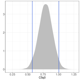
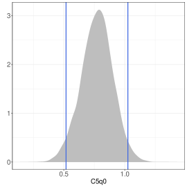
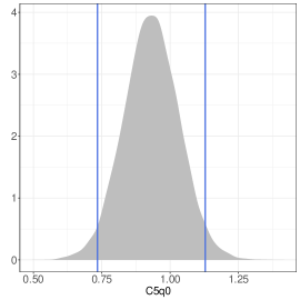
Both sexes (Gamma)	Females (Gamma)	Males (Gamma)

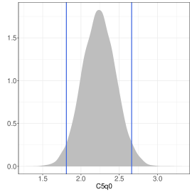
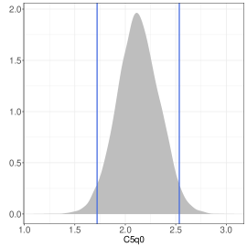
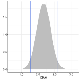
Figure 1. Marginal posterior of C5q0 with quantile-based credible intervals in blue lines for model 1 considering both sexes, females and males with LA prior for the local scales of the random effects and local Half-Cauchy and a common Gamma prior for the scale of the errors respectively.

Table 2. R-squared, RMSE and MAE for the considered models using different HS, LA and Student-t priors for the local scales of the random effects and a common Gamma prior for the scale of the random effects and errors respectively (without Global-Local structure). Frequentist refers to the original model proposed in Adair and Lopez (2018) fitted using restricted maximum likelihood estimation.

Prior for the errors: Gamma
				Model 1					Model 2
		Frequentist	Gamma	Student-t	HS	LA	Frequentist	Gamma	Student-t	HS	LA
Both sexes	R-square	0.8360	0.8362	0.8348	0.8370	0.8386	0.7894	0.7895	0.7930	0.7947	0.7982
	RMSE	2.6172	2.6171	2.6276	2.6319	2.6612	2.6153	2.6154	2.6210	2.6225	2.6449
	MAE	4.2804	4.2795	4.2971	4.3016	4.3384	4.4552	4.4558	4.4701	4.4738	4.5268
Females	R-square	0.8477	0.8474	0.8454	0.8461	0.8432	0.8108	0.8104	0.8145	0.8151	0.8206
	RMSE	2.6380	2.6389	2.6505	2.6564	2.6974	2.6459	2.6466	2.6546	2.6589	2.7088
	MAE	4.2391	4.2398	4.2564	4.2636	4.3160	4.3755	4.3778	4.4007	4.4100	4.5087
Males	R-square	0.8227	0.8229	0.8222	0.8243	0.8261	0.7795	0.7795	0.7851	0.7883	0.7971
	RMSE	2.7053	2.7041	2.7132	2.7180	2.7483	2.7841	2.7831	2.7896	2.7938	2.8163
	MAE	4.3582	4.3566	4.3691	4.3759	4.4143	4.6852	4.6842	4.6895	4.6999	4.7435

Table 3. R-squared, RMSE and MAE for the considered models using different Gamma, HS, LA and Student-t priors for the local scales of the random effects and a Half-Cauchy for the local scale of the errors and a common Gamma for the scale of the random effects, respectively. Frequentist refers to the original model proposed in Adair and Lopez (2018) fitted using restricted maximum likelihood estimation.

Prior for the errors: Local prior - Half-Cauchy and Global prior - Gamma
				Model 1					Model 2
		Frequentist	Gamma	Student-t	HS	LA	Frequentist	Gamma	Student-t	HS	LA
Both sexes	R-square	0.836	0.795	0.799	0.805	0.827	0.789	0.802	0.807	0.808	0.815
	RMSE	2.617	2.329	2.332	2.334	2.349	2.615	2.477	2.480	2.482	2.494
	MAE	4.280	3.863	3.866	3.872	3.900	4.455	4.199	4.206	4.209	4.230
Females	R-square	0.848	0.826	0.828	0.829	0.830	0.811	0.825	0.830	0.829	0.832
	RMSE	2.638	2.399	2.404	2.409	2.450	2.646	2.507	2.510	2.515	2.542
	MAE	4.239	3.873	3.877	3.889	3.964	4.376	4.144	4.157	4.163	4.215
Males	R-square	0.823	0.783	0.793	0.803	0.822	0.780	0.790	0.793	0.797	0.798
	RMSE	2.705	2.385	2.389	2.392	2.412	2.784	2.585	2.586	2.587	2.593
	MAE	4.358	3.901	3.904	3.911	3.934	4.685	4.382	4.383	4.387	4.386

However, the posterior mean of the constant parameter and C5q0 are slightly different when Gamma and Half-Cauchy priors are considered for the local scale of the errors. Figure 1 illustrates that the posterior mean of C5q0 is around 0.75 and 2.2 when a local Half-Cauchy and a common Gamma prior is considered for scales of the errors, respectively. This suggests that models using the Gamma prior are less sensitive to the completeness of under-five death registration when compared to those using the Half-Cauchy prior. Considering GL priors for the errors and random effects in both models 1 and 2 improves the estimation of the completeness of death registration. This is illustrated in Tables 3-3 where there are important reductions in terms of RMSE and MAE when a Half-Cauchy prior is considered for the scale of the errors in model (2.1) and implemented in models 1 and 2 and for both sexes, males and females. The differences of RMSE and MAE are practically negligible when Gamma, Student-t, HS or LA priors are considered for the local scales of the random effects. Interesting, similar values of RMSE, MAE and R-square are obtained under the HS and the local Student-t priors likely due to the similar tail behavior in the resulting marginal posterior distribution of the random effects.

Model 1 (Both sexes)	Model 2 (Both sexes)

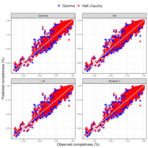
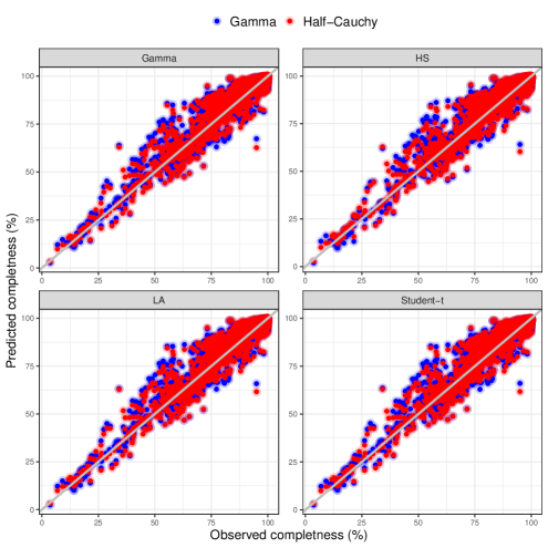
Figure 2. Posterior predicted mean versus observed death registration completeness, and using HS LA and Student-t priors for the local scales of the random effects and a Half Cauchy prior for the local scale of the errors and common Gamma distributions for the random effects and errors respectively. The models are based on an dataset updated to 2019, which uses GBD death estimates based on the GBD 2019 and comprises 120 countries and 2,748 country-years from 1970-2019 (Demographics Collaborators, 2020). Both sexes with model 1 and model 2.

As we expected, similar but larger values of the RMSE and MAE are obtained by considering the Frequentist model and the Bayesian model under a common Gamma prior for the scales of the random effects and errors, respectively. However, when LA priors are considered for the random effects the R-square values are higher and around 80% of those obtained with Gamma, Student-t and HS local priors and similar of those obtained with the frequentist (and the Bayesian approach) model. This result shows that the use of GL priors rather than a common Gamma priors is crucial because observed completeness and covariates may exhibit considerable inter-country variability. This result also supports that the use of Half-Cauchy priors for the local scales of the errors rather than a common Gamma prior is particularly important because observed completeness may exhibit considerable within-country variability, particularly for the 30%-90% completeness range where the data is concentrated. This is illustrated in Figure  2 where a large amount of the observed completeness is between around 30% to 90%.

Model 1 - Half-Cauchy (Both Sexes)	Model 1 - Gamma (Both Sexes)

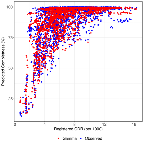
Figure 3. Predicted versus observed death registration completeness by registered CDR Student-t priors for the local scales of the random effects.The models are based on an dataset updated to 2019, which uses GBD death estimates based on the GBD 2019 and comprises 120 countries and 2,748 country-years from 1970-2019 (Demographics Collaborators, 2020). Model 1, both sexes with Half-Cauchy and Gamma priors for the scales, respectively.

Figure  2 also displays how GL priors and the completeness of registered under-five deaths as a predictor dramatically improves the estimation over this range of completeness. This is also confirmed in Tables  4 and  5 where the suitable posterior predictive estimates of completeness are obtained according to the RMSE and MAE. Taking a closer look at the results for ranges of observed completeness between 0% to 30% for model 1 and for both sexes and males, the MAE values are lower when a Gamma prior is considered for the scale of the errors of the random effects. However, for other models and also for higher completeness levels the reduction in terms of RMSE and MAE is large when a Half-Cauchy prior is considered for the scale of the errors for each country $i=1,...,m$. The predictor RegCDR shows a curvilinear relationship with observed completeness, as was first pointed out by (Adair and Lopez, 2018), and in this paper the posterior predictive mean estimates also show this relationship.

Importantly, Figure  3 (left) for Half-Cauchy priors illustrates how the observed variability of the registered CDR in the completeness range 30% to 90% is captured for the proposed models, with the posterior predictive mean estimates and observed completeness close to each other. This range of completeness is particularly important because for these populations the method has greatest utility (i.e. where completeness is above 90% there is more certainty about the true level of completeness, while where completeness is less than 30% it is not recommended to use estimated completeness to adjust mortality rates). This makes Half-Cauchy priors suitable choices for the scale of the errors.

Global-Prior		Gamma				Half-Cauchy
Local-Prior	Gamma	Student-t	HS	LA	Gamma	Student-t	HS	LA
Model 1 (both sexes)
90$<$100	1.87	1.88	1.88	1.90	1.96	1.97	1.97	2.00
80$<$90	5.36	5.37	5.37	5.36	4.83	4.83	4.82	4.76
60$<$80	7.92	7.94	7.93	7.95	6.85	6.88	6.89	6.96
30$<$60	9.14	9.21	9.26	9.48	7.71	7.66	7.71	7.91
$<$30	4.67	4.77	4.86	5.34	6.12	6.12	6.08	5.96
Model 2 (both sexes)
90$<$100	2.08	2.09	2.09	2.10	2.11	2.13	2.13	2.15
80$<$90	5.10	5.09	5.08	5.00	4.98	4.97	4.96	4.89
60$<$80	7.33	7.35	7.37	7.49	6.88	6.88	6.89	6.92
30$<$60	10.10	10.15	10.19	10.48	9.00	9.04	9.06	9.22
$<$30	4.84	4.84	4.80	4.71	4.13	4.14	4.12	4.15
Model 1 (females)
90$<$100	1.89	1.91	1.91	1.95	1.95	1.97	1.97	1.99
80$<$90	5.42	5.43	5.43	5.47	4.96	4.97	4.98	5.04
60$<$80	7.80	7.82	7.82	7.81	6.96	6.97	6.99	7.18
30$<$60	8.53	8.57	8.62	8.83	7.20	7.13	7.19	7.40
$<$30	5.15	5.33	5.38	5.99	5.91	5.94	5.92	5.66
Model 2 (females)
90$<$100	2.06	2.08	2.07	2.10	2.07	2.09	2.09	2.11
80$<$90	5.26	5.27	5.28	5.30	5.13	5.14	5.14	5.15
60$<$80	7.26	7.30	7.31	7.44	6.92	6.92	6.93	7.01
30$<$60	9.70	9.78	9.83	10.26	8.65	8.68	8.71	8.89
$<$30	4.34	4.29	4.32	4.44	3.80	3.83	3.84	4.04
Model 1 (males)
90$<$100	1.90	1.92	1.92	1.96	1.97	1.98	1.99	2.04
80$<$90	5.24	5.24	5.24	5.24	4.69	4.70	4.70	4.67
60$<$80	7.94	7.96	7.95	7.93	6.91	6.93	6.94	6.99
30$<$60	8.69	8.73	8.80	9.06	7.29	7.22	7.25	7.25
$<$30	5.39	5.41	5.46	5.71	5.62	5.61	5.56	5.66
Model 2 (males)
90$<$100	2.12	2.13	2.14	2.18	2.15	2.16	2.17	2.23
80$<$90	5.05	5.05	5.04	4.98	4.82	4.82	4.80	4.73
60$<$80	7.72	7.73	7.73	7.77	7.39	7.39	7.37	7.33
30$<$60	10.27	10.27	10.36	10.64	8.73	8.71	8.76	8.82
$<$30	6.24	6.22	6.19	5.94	5.91	5.88	5.88	5.82

Table 4. RMSE measures and sensitivity analysis of the Half-Cauchy local scale prior and a common Gamma prior for the errors in model 1 and 2 considering different levels of completeness.

Global-Prior		Gamma				Half-Cauchy
Local-Prior	Gamma	Student-t	HS	LA	Gamma	Student-t	HS	LA
Model 1 (both sexes)
90$<$100	1.18	1.18	1.18	1.18	1.18	1.19	1.19	1.20
80$<$90	4.49	4.48	4.49	4.47	3.79	3.79	3.78	3.72
60$<$80	6.63	6.67	6.67	6.72	5.47	5.49	5.51	5.59
30$<$60	6.90	7.01	7.07	7.45	5.53	5.53	5.56	5.70
$<$30	3.78	3.87	3.91	4.11	4.74	4.76	4.74	4.68
Model 2 (both sexes)
90$<$100	1.25	1.25	1.25	1.25	1.24	1.24	1.24	1.25
80$<$90	3.99	3.98	3.98	3.94	3.85	3.85	3.84	3.79
60$<$80	5.66	5.68	5.69	5.80	5.22	5.22	5.23	5.27
30$<$60	7.47	7.52	7.53	7.73	6.64	6.67	6.69	6.83
$<$30	3.33	3.40	3.41	3.35	2.95	2.98	2.98	3.03
Model 1 (females)
90$<$100	1.24	1.24	1.25	1.26	1.26	1.26	1.26	1.27
80$<$90	4.50	4.51	4.51	4.55	3.94	3.94	3.95	4.01
60$<$80	6.39	6.41	6.41	6.44	5.39	5.40	5.42	5.53
30$<$60	6.59	6.68	6.75	7.07	5.50	5.51	5.55	5.84
$<$30	4.34	4.48	4.51	4.89	4.73	4.77	4.76	4.66
Model 2 (females)
90$<$100	1.32	1.32	1.32	1.33	1.30	1.30	1.30	1.31
80$<$90	4.15	4.16	4.18	4.27	3.98	3.99	3.99	4.03
60$<$80	5.60	5.63	5.63	5.74	5.20	5.19	5.20	5.24
30$<$60	7.36	7.39	7.41	7.63	6.53	6.55	6.59	6.75
$<$30	3.58	3.53	3.54	3.54	3.20	3.21	3.22	3.33
Model 1 (males)
90$<$100	1.20	1.20	1.20	1.21	1.19	1.20	1.20	1.22
80$<$90	4.38	4.38	4.39	4.40	3.68	3.69	3.69	3.68
60$<$80	6.61	6.65	6.64	6.66	5.51	5.53	5.54	5.58
30$<$60	6.29	6.35	6.43	6.80	5.16	5.16	5.17	5.21
$<$30	4.59	4.64	4.66	4.73	4.24	4.23	4.21	4.27
Model 2 (males)
90$<$100	1.29	1.29	1.30	1.31	1.26	1.26	1.27	1.29
80$<$90	3.89	3.89	3.88	3.87	3.69	3.69	3.68	3.64
60$<$80	5.96	5.98	5.98	6.03	5.66	5.66	5.66	5.61
30$<$60	7.85	7.87	7.91	8.06	6.25	6.26	6.28	6.38
$<$30	3.95	4.03	4.06	3.94	3.02	3.02	3.02	3.05

Table 5. MAE measures and sensitivity analysis of the Half-Cauchy local scale prior and a common Gamma prior for the errors in model 1 and 2 considering different levels of completeness..

To illustrate that the inclusion of GL priors affect the predictions of the logit of completeness we consider two deviances at the country and at the country-year levels with

$$\text{Deviance}^{\text{countr- level}} =(\bar{y}_{i}-\bm{\bar{x}_{i}^{\textsf{T}}}\hat{\bm{\beta}})^{2}, \text{Deviance}^{\text{country-year level}} =\sum\limits_{j=1}^{n_{i}}(y_{ij}-\bm{x_{ij}}^{T}\hat{\bm{\beta}})^{2}/n_{i}$$

where $\hat{\bm{\beta}}$ denotes the ordinary least squares estimates from a multiple regression model. Notice that these two deviances in some sense measure the within country and between country-year variabilities. According to Theorem 2.1 when the difference $|\bar{\bm{y}}_{i}-\bar{\bm{x}}_{i}^{\textsf{T}}\bm{\beta}_{i}|$ increases then the shrinkage under the posterior mean of the random effects towards zero is offset and the random effects depend on the observed completeness and the regression fit. This is illustrated in Figure 4 where the random effects increases under GL priors with the deviance at the country-level. However as is pointed out in Theorem 2.1 the posterior concentration of the shrinkage factors are also affected for the GL priors of the errors. Notice that the shape of the conditional Gamma posterior distribution of the global parameter $\tau$ in algorithm 2 depends on the country-year level variability. This behavior is also illustrated in Figure 4 where the values of the random effects under GL priors are very sensible even to smaller values of within country-year variability.

Both sexes	Females	Males

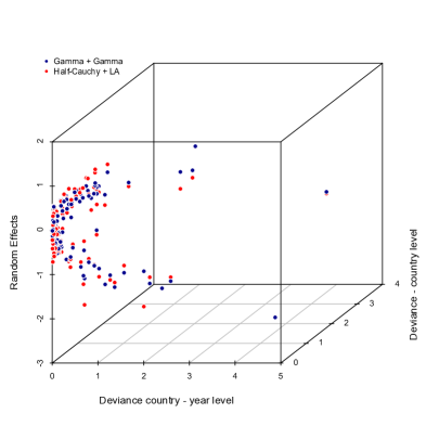
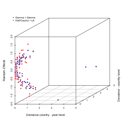
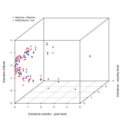
Figure 4. Posterior means of random effects from model 1 using the LA local prior for the scales of the random effects and a common Gamma or a Half-Cauchy prior for the scales of the errors versus the deviances at country and country - year levels.

5. National and subnational implementation: completeness of death registration in Colombia and its Departments in 2017

To evaluate the performance and demonstrate the utility of the models in Section 4, in this section we use them to estimate the completeness of death registration $c_{k}$ for both sexes, males and females for the Country of Colombia and the corresponding regional division by 33 departments in 2017, $k=1,...,33$. The results are compared to data from the Colombian population census described earlier. We call the estimates from the Census the observed estimates $c_{k}$ during for the purpose of analysis of the results. The models estimated completeness of deaths in 2017 from vital registration, the same data source for which Census respondents report whether a household death was registered (DANE, 2017a). The 5q0 was estimated considering the same procedure implemented in Adair and Lopez (2018); we considered the average from the 2010 and 2015 Demographic and Health Surveys (DHS, 2010, 2015) and scaled those estimates to the GBD of 5q0 for Colombia in 2017. We consider the projected values of population aged 65 years and over in 2017 using the official population projections in Colombia (DANE, 2017b). To estimate C5q0 we computed the ratio between the 5q0 obtained from standard life tables using the registration data (DANE, 2017a) divided by the estimate of 5q0 as in Adair and Lopez (2018).

Table 6. MAE, MSE, and the number of departments including national level with absolute deviations of the predictive completeness $\hat{\delta}_{k}$ and the comparator $c_{k}$ less than10 percentage points. The table contains the results for HS, LA and Student-t local scale priors for the random effects and the Half-Cauchy for the local scale of the errors and common Gamma prior for the scale of the random effects and errors, respectively.

A common prior for the scale of the errors: Gamma
			Model 1				Model 2
		Gamma	Student-t	HS	LA	Gamma	Student-t	HS	LA
			Model 1				Model 2
	MAE	0.060	0.054	0.061	0.060	0.054	0.054	0.053	0.054
Both sexes	MSE	0.009	0.006	0.010	0.009	0.006	0.006	0.006	0.006
	# diff¡10%	29	28	28	29	29	28	29	28
	MAE	0.062	0.062	0.062	0.062	0.054	0.055	0.052	0.054
Males	MSE	0.009	0.009	0.009	0.009	0.006	0.006	0.005	0.006
	# diff¡10%	29	29	28	29.000	30	30	30	30
	MAE	0.059	0.059	0.061	0.060	0.052	0.052	0.054	0.052
Females	MSE	0.010	0.010	0.010	0.010	0.005	0.005	0.006	0.005
	# diff¡10%	29	29	29	30	28	28	29	28

Local scale prior for the errors: Half-Cauchy
			Model 1				Model 2
		Gamma	Student-t	HS	LA	Gamma	Student-t	HS	LA
	MAE	0.055	0.045	0.053	0.054	0.045	0.045	0.046	0.045
Both sexes	MSE	0.008	0.004	0.008	0.008	0.004	0.004	0.004	0.004
	# diff¡10%	29	30	30	29	30	30	30	30
	MAE	0.056	0.056	0.055	0.055	0.047	0.047	0.048	0.047
Males	MSE	0.008	0.007	0.007	0.007	0.005	0.005	0.005	0.005
	# diff¡10%	30	30	30	30	29	29	30	30
	MAE	0.053	0.052	0.051	0.052	0.048	0.048	0.048	0.048
Females	MSE	0.008	0.008	0.007	0.008	0.005	0.005	0.005	0.005
	# diff¡10%	30	30	30	30	30	29	29	29

To evaluate the fit of the models at the national and subnational level (the national level and the 33 departments) we consider two deviance measures, the MAE and the Mean Square Error (MSE) given by,

(5.1) MAE $$=\dfrac{1}{34}\sum_{k=1}^{34}\mid\hat{\delta}_{k}-c_{k}\mid, =\dfrac{1}{34}\sum_{k=1}^{34}(\hat{\delta}_{k}-c_{k})^{2},$$ MSE

where $\hat{\delta}_{k}$ is the posterior mean of the posterior predictive distribution. We also compute the number of departments with absolute deviations $\mid\hat{\delta}_{k}-c_{k}\mid$ smaller than 10 percentage points. Table  6 shows that in 29 or 30 departments and at the national level the absolute deviances between the observed completeness $c_{k}$ and the posterior predictive mean estimate is less than 10 percentage points for the models considering a Half-Cauchy prior for the local scale of the errors (depending on the local prior).

Model 1 (Both Sexes)	Model 2 (Both Sexes)

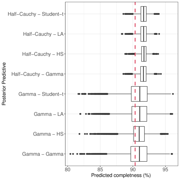
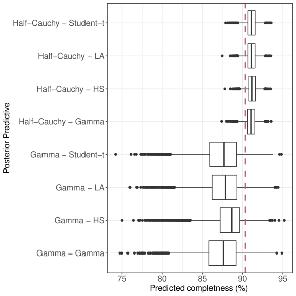
Figure 5. Marginal posterior predictive distributions of the completeness at national level under Gamma, Student-t, HS and LA local scales for the random effects and Half-Cauchy for the local scales of the errors, Gamma-Gamma refers to the model with a common Gamma prior distribution for the random effects and errors respectively, Model 1 and 2, both sexes. The red lines illustrates the observed values obtained from Census 2018.

Model 1 (Males)	Model 2 (Males)

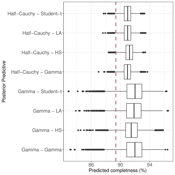
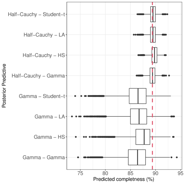
Figure 6. Marginal posterior predictive distributions of the completeness at national level under Gamma, Student-t, HS and LA local scales for the random effects and Half-Cauchy for the local scales of the errors, Gamma-Gamma refers to the model with a common Gamma prior distribution for the random effects and errors respectively, Model 1 and 2, males. The red lines illustrates the observed values obtained from Census 2018.

In addition, there are important reductions in terms of MAE and MSE and slightly better posterior predictive estimates are obtained when the HS is considered as a local scale for the random effects compared with the Gamma prior distribution. We also illustrate the posterior predictive distributions in Figures  5- 7 at the national level. The inclusion of Half-Cauchy as a local-scale prior under the errors that control the shrinkage under the posterior mean of the random effects makes a substantial difference. The posterior predictive distributions obtained at the national level are more precise in these Figures. In addition the posterior predictive mean is closer to the observed completeness at the National level in Colombia for 2017. These results are also observed for both sexes, males and females and models 1 and 2. Further, the HS prior for the local scales of random effects produces posterior predictive estimates closer to the observed completeness with higher precision than the other local scale priors, as is displayed in Figures  5- 7.

Model 1 (Females)	Model 2 (Females)

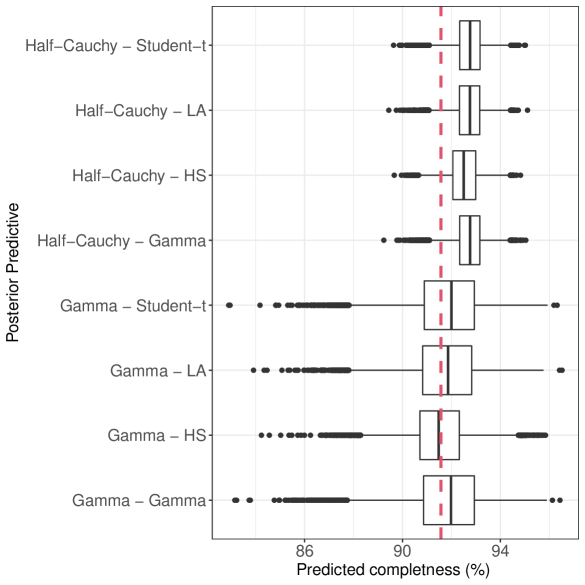
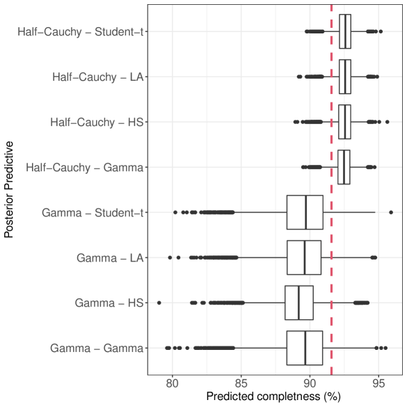
Figure 7. Marginal posterior predictive distributions of the completeness at national level under Gamma, Student-t, HS and LA local scales for the random effects and Half-Cauchy for the local scales of the errors, Gamma-Gamma refers to the model with a common Gamma prior distribution for the random effects and errors respectively, Model 1 and 2, females. The red lines illustrates the truth values obtained from Census 2018.

Table 7 and Tables 14-17 in the supplementary material in Section 11 show the posterior predictive mean estimates and the corresponding credible intervals for models 1 and 2 both sexes, females and males, respectively. As is presented in Tables 7 and 14-17 most of the posterior mean estimates are closer to the observed value of completeness in the departments of Colombia in 2017 and for almost all departments the credible intervals under GL priors contain the observed completeness. These important results are also obtained when models 1 and 2 are considered for females and males as shown in Tables 14-17. Departments such as Chocó, Amazonas, Vaupés and La Guajira with some of the higher mortality rates and historically affected by problems in the civil registration system present important lower values of completeness according to Census. Considering GL priors for the random effects and errors in models 1 and 2 allow us to obtain posterior predictive estimates closer to the observed completeness for those departments. Figure 8 displays the spatial patterns of the observed completeness according to the Census 2018 in Colombia and posterior predictive estimates obtained by considering a HS prior for the scales of the random effects and a Half-Cauchy prior for scale of the errors. As is illustrated in the Figures, Vaupés, Guainía, Vichada, Amazonas, La Guajira and Chocó have lower completeness values of death registration observed in the Census. Those completeness patterns in the departments of Colombia are also effectively estimated by considering the proposed models. Model 2 with respect to Model 1 for both sexes, females and males produce posterior predictive completeness estimates slightly closer (for those departments) to the obtained considering the comparator from Census.

					Model 1 (Both Sexes)
Department	Census	Gamma	$2.5\%$	$97.5\%$	Student-t	$2.5\%$	$97.5\%$	LA	$2.5\%$	$97.5\%$	HS	$2.5\%$	$97.5\%$
Antioquia	92	95	94	96	95	94	96	95	94	96	95	94	96
Atlántico	96	94	92	95	94	92	94	94	92	94	94	92	94
Bogotá, D.C.	96	92	91	93	92	91	93	92	91	93	92	91	93
Bolívar	88	90	89	92	90	89	92	90	89	92	90	89	91
Boyacá	93	93	91	94	93	91	94	93	91	94	93	92	94
Caldas	93	97	97	98	98	97	98	98	97	98	98	97	98
Caquetá	87	93	92	94	93	92	94	93	92	94	93	92	94
Cauca	83	86	84	88	86	84	88	86	84	88	86	84	87
Cesar	88	84	81	86	83	81	86	83	81	86	83	81	85
Córdoba	88	86	84	88	86	84	88	86	84	88	86	84	88
Cundinamarca	93	96	95	96	96	95	96	96	95	96	96	95	96
Chocó	65	61	56	66	61	56	66	61	56	65	58	54	63
Huila	92	91	89	92	91	89	92	91	89	92	91	90	92
La Guajira	39	52	46	57	51	46	56	51	45	56	48	43	52
Magdalena	88	90	88	91	90	88	91	90	88	91	89	88	91
Meta	91	96	95	97	96	95	97	96	95	97	96	96	97
Nariño	82	85	82	87	85	83	87	85	83	87	85	83	87
Norte de Santander	90	93	91	94	93	91	94	93	91	94	93	92	93
Quindio	94	96	95	96	96	95	96	96	95	96	96	95	96
Risaralda	93	96	96	97	96	96	97	96	96	97	97	96	97
Santander	94	92	91	93	92	91	93	92	91	93	92	91	93
Sucre	86	93	92	94	93	92	94	93	92	94	93	92	94
Tolima	91	91	89	92	91	89	92	91	89	92	91	89	92
Valle del Cauca	95	96	95	96	96	95	96	96	95	96	96	95	97
Arauca	85	96	95	97	96	95	97	96	95	97	96	96	97
Casanare	87	94	93	95	94	93	95	94	93	95	94	93	95
Putumayo	79	84	81	86	83	81	86	83	81	85	83	81	85
San Andrés	93	95	94	96	95	94	96	95	94	96	95	94	96
Amazonas	67	70	66	74	70	66	74	70	66	73	68	65	71
Guainía	51	87	84	89	86	83	89	86	83	88	86	83	88
Guaviare	81	94	93	95	94	93	95	94	93	95	94	93	95
Vaupés	57	60	56	65	60	55	64	59	55	64	57	54	61
Vichada	60	86	83	88	86	82	88	85	82	88	85	82	87
National	90	92	90	93	92	90	93	92	90	93	92	90	93

					Model 2 (Both Sexes)
Department	Census	Gamma	$2.5\%$	$97.5\%$	Student-t	$2.5\%$	$97.5\%$	LA	$2.5\%$	$97.5\%$	HS	$2.5\%$	$97.5\%$
Antioquia	92	95	94	95	95	94	95	95	94	95	95	94	95
Atlántico	96	92	91	93	92	91	93	92	91	93	92	91	93
Bogotá, D.C.	96	91	90	92	91	90	92	91	90	92	91	90	92
Bolívar	88	88	86	89	88	86	89	88	86	89	88	86	89
Boyacá	93	93	92	94	93	92	94	93	92	94	93	92	94
Caldas	93	97	97	98	97	97	98	97	97	98	98	97	98
Caquetá	87	92	91	93	92	91	93	92	91	93	92	91	93
Cauca	83	84	82	86	84	82	86	84	82	86	84	82	86
Cesar	88	80	78	82	80	77	82	80	77	82	80	77	82
Córdoba	88	83	80	85	83	80	85	83	80	85	83	81	85
Cundinamarca	93	94	94	95	95	94	95	95	94	95	95	94	95
Chocó	65	53	48	57	53	48	57	52	48	57	52	47	56
Huila	92	92	90	93	92	90	93	92	90	93	92	90	93
La Guajira	39	46	41	51	45	41	50	45	40	50	44	40	48
Magdalena	88	86	85	88	86	85	88	86	85	88	86	85	88
Meta	91	95	94	95	95	94	95	95	94	95	95	94	95
Nariño	82	86	83	88	86	83	88	86	83	88	86	84	88
Norte de Santander	90	93	92	94	93	92	94	93	92	94	93	92	94
Quindio	94	96	95	97	96	95	97	96	95	97	96	96	97
Risaralda	93	96	96	97	96	96	97	96	96	97	96	96	97
Santander	94	93	92	94	93	92	94	93	92	94	93	92	94
Sucre	86	91	90	92	91	90	92	91	90	92	91	90	92
Tolima	91	93	91	94	93	91	94	93	92	94	93	92	94
Valle del Cauca	95	96	95	97	96	95	97	96	95	97	96	96	97
Arauca	85	95	94	95	95	94	95	95	94	95	95	94	95
Casanare	87	91	90	92	91	90	92	91	90	92	91	90	92
Putumayo	79	82	80	85	82	80	84	82	80	84	82	80	84
San Andrés	93	94	93	94	94	93	94	94	93	94	94	93	94
Amazonas	67	63	59	67	63	59	67	63	59	67	62	59	66
Guainía	51	75	72	78	75	72	78	75	72	78	75	72	78
Guaviare	81	92	90	93	92	90	93	92	90	93	92	91	93
Vaupés	57	55	51	59	55	50	59	54	50	59	54	50	58
Vichada	60	73	69	76	73	69	76	73	69	76	72	69	76
National	90	91	90	92	91	90	92	91	90	92	91	90	92

Table 7. Posterior predictive estimates and 95% credible intervals under Gamma, HS, LA and Student-t local priors for the random effects and a Half-Cauchy local prior for the scale of the errors and the observed estimates from the census. Inf and Sup represent the 2.5% and 97.5% quantiles from the marginal posterior distribution of the completeness in each Department and at the national level. Both Sexes and models 1 and 2.

Census 2018 (Both-sexes)	Model 1 (Both Sexes)	Model 2 (Both Sexes)
	HS + Half-Cauchy	HS + Half-Cauchy
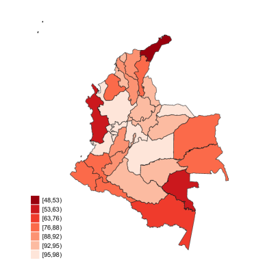
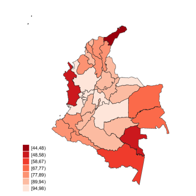
Census 2018 (Female)	Model 1 (Female)	Model 2 (Female)
	HS + Half-Cauchy	HS + Half-Cauchy
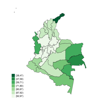
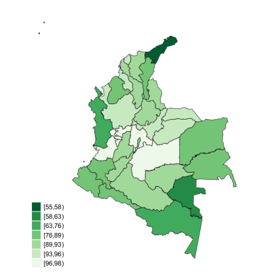
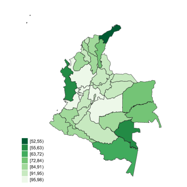
Census 2018 (Male)	Model 1 (Male)	Model 2 (Male)
	HS + Half-Cauchy	HS + Half-Cauchy

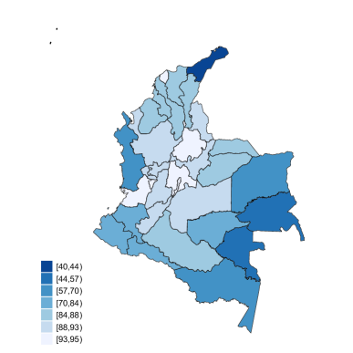
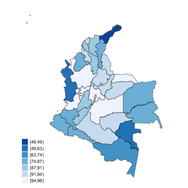
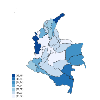
Figure 8. Completeness of death registration at departmental level in Colombia according to Census 2018 (left), Bayesian Model 1 (middle) and Bayesian model 2 (right) with HS priors for the local scales of the random effects and a Half-Cauchy for the local scales of the errors by both sexes, females and males.

6. Concluding remarks and discussion

In this work we propose the use of GL priors in this paper for situations where demographic covariates can explain much of the observed completeness but where unexplained within-country (i.e. by year) and between-country variability also plays an important role. Therefore, we introduce GL priors for the scales of the random effects and errors respectively in hierarchical linear mixed models to estimate the completeness of death registration and study their theoretical properties to allow small and large random effects when it is required. Our proposal is inspired by the original model proposed by Adair and Lopez (2018) which includes information typically available from multiple sources, e.g., surveys, censuses and administrative records.

The use of a Bayesian framework with GL priors to extend the existing Adair and Lopez (2018) models further strengthens the models effectiveness at estimating completeness of death registration. These models are immensely useful to enable estimation of completeness of death registration in a timely manner using available data, as demonstrated by their wide use in several different settings (Zeng et al., 2020; Sempé et al., 2021; Adair et al., 2021). In particular, they overcome the limitations of existing methods which rely on inaccurate assumptions of population dynamics and often provide estimates that lack timeliness. Furthermore, this paper uses an updated GBD dataset using data to 2019 from 120 countries and 2,748 country-years and also improves the model’s ability to predict completeness in contemporary populations.

A limitation of the use of the Colombia Census as a comparator is that the data are based on households responding to a question about whether reported deaths, which comprise about 90% of total deaths in the country, were registered. These figures may differ from actual death registration because of incorrect recollection by the household, whether intentional or otherwise, and also if death registration status of the 10% of unreported deaths differ substantially from the 90% of deaths that are reported. However the similarity in results for the predicted registration completeness and the completeness reported in the Census suggests that any such issues are minimal.

We also proposed new Markov chain Monte Carlo (MCMC) algorithms for hierarchical linear mixed models under GL priors to estimate the uncertainty of the estimated completeness of the death registration at the global, national and subnational levels. Finally, the methodological results in this paper are complementary to existing alternatives under GL priors and can be implemented in a general framework to estimate other demographic indicators at subnational levels.

7. Proof of Theorems

We consider in this section the proofs of Theorems 3.1 and 2.1.

7.1. Proof of Theorem 3.1

Proof.

Consider model (2.1) in matrix form as follow

(7.1) $$\bm{y_{i}} =\bm{X_{i}}\bm{\beta}+u_{i}\bm{1}_{n_{i}}+\bm{\epsilon_{i}}, i=1,...,m,$$

where $\bm{y_{i}}=(y_{i1},...,y_{in_{i}})^{\textsf{T}}$, $\bm{X_{i}}=(\bm{x}_{i1},...,\bm{x}_{in_{i}})^{\textsf{T}}$, $\bm{\epsilon_{i}}=(\bm{\epsilon}_{i1},...,\bm{\epsilon}_{in_{i}})^{\textsf{T}}$, $\bm{u}=(u_{1},...,u_{m})^{\textsf{T}}$. The joint posterior density can be written as follow

$$p(\bm{u},\phi,\bm{\omega},\bm{\beta},\tau,\bm{\lambda}\mid\bm{y}) \propto\prod_{i=1}^{m}|(\lambda_{i}\tau)^{-1}I_{m})|^{-1/2}\exp\left\{-\frac{1}{2}(\bm{z_{i}}-\bm{X_{i}}\bm{\beta})^{\textsf{T}}(\lambda_{i}\tau)I_{m}(\bm{z_{i}}-\bm{X_{i}}\bm{\beta})\right\}$$

(7.2) $$\hskip 28.45274pt\times(\omega_{i}\phi)^{1/2}\exp\left\{-\frac{1}{2}u_{i}^{2}\omega_{i}\phi\right\}\pi(\tau)\pi(\lambda_{i})\pi(\phi)\pi(\omega_{i}).$$

Consider now the block-diagonal structure for model (7.1) given by

$$\bm{z} =\text{col}_{1\leq i\leq m}(\bm{z_{i}})=(\bm{z_{1}}^{\textsf{T}},...,\bm{z_{m}})^{\textsf{T}}, \bm{X} =\text{col}_{1\leq i\leq m}(\bm{X_{i}^{\textsf{T}}}),$$

$$\bm{V} =\text{blkdiag}(\{\bm{V_{i}}\}_{i=1}^{m}), \bm{\epsilon} =\text{col}_{1\leq i\leq m}(\bm{\epsilon_{i}}),$$

where $\bm{z_{i}}=\bm{y_{i}}-u_{i}\bm{1}_{n_{i}}$ and $\bm{V_{i}}=(\lambda_{i}\tau)I_{m}$. Since $\bm{X}$ is of full range then $\bm{X}^{\textsf{T}}\bm{V}\bm{X}$ is nonsingular. Notice that

$$\exp\left\{-\frac{1}{2}(\bm{z}-\bm{X}\bm{\beta})^{\textsf{T}}\bm{V}(\bm{z}-\bm{X}\bm{\beta})\right\}$$

$$=\exp\left\{-\frac{1}{2}(\bm{\beta}-\hat{\bm{\beta}})^{\textsf{T}}\bm{X}^{\textsf{T}}\bm{V}\bm{X}(\bm{\beta}-\hat{\bm{\beta}})-\frac{1}{2}(\bm{z}-\bm{X}\hat{\bm{\beta}})^{\textsf{T}}\bm{V}(\bm{z}-\bm{X}\hat{\bm{\beta}})\right\}$$

where $\hat{\bm{\beta}}=(\bm{X}^{\textsf{T}}\bm{V}\bm{X})^{-1}\bm{X}^{\textsf{T}}\bm{V}\bm{z_{i}}$. Computing the integral of the right-hand site in (7.1) with respect to $\bm{\beta}$ and having that $\exp\left\{-\frac{1}{2}(\bm{z}-\hat{\bm{\beta}})^{\textsf{T}}\bm{V}(\bm{z}-\hat{\bm{\beta}})\right\}\leq 1$ then

(7.3) $$p(\bm{u},\phi,\bm{\omega},\tau,\bm{\lambda}\mid\bm{y}) \leq K\prod_{i=1}^{m}(\omega_{i}\phi)^{1/2}\exp\left\{-\frac{1}{2}u_{i}^{2}\omega_{i}\phi\right\}\pi(\tau)\pi(\lambda_{i})\pi(\phi)\pi(\omega_{i}),$$

where $K$ is a generic positive constant. Integrating (7.3) with respect to $\bm{u}$, we have

(7.4) $$p(\phi,\bm{\omega},\bm{\beta},\tau,\bm{\lambda}\mid\bm{y}) \leq K\prod_{i=1}^{m}\pi(\tau)\pi(\lambda_{i})\pi(\phi)\pi(\omega_{i}),$$

moreover if the priors distributions of $\pi(\tau)$, $\pi(\lambda_{i})$, $\pi(\phi)$ and $\pi(\omega_{i})$ are proper then the posterior distribution is proper. ∎

7.2. Proof of Theorem 2.1

Proof.

For (i) consider

(7.5) $$\small P(\gamma_{i}>\epsilon\mid\bm{\beta},\bm{\lambda},\tau,\bm{y}_{i})=\dfrac{\bigintss_{0}^{c_{1}/\phi}N(\bm{y_{i}};\bm{X_{i}}\bm{\beta},I_{m}(\lambda_{i}\tau)^{-1}+\bm{1}_{n_{i}}\bm{1}_{n_{i}}^{\textsf{T}}(\omega_{i}\phi)^{-1})\pi(\omega_{i})d\omega_{i}}{\bigintss_{0}^{\infty}N(\bm{y_{i}};\bm{X_{i}}\bm{\beta},I_{m}(\lambda_{i}\tau)^{-1}+\bm{1}_{n_{i}}\bm{1}_{n_{i}}^{\textsf{T}}(\omega_{i}\phi)^{-1})\pi(\omega_{i})d\omega_{i}}=\dfrac{N_{1}}{D_{1}},$$

where $c_{1}=((1-\epsilon)/\epsilon)(n_{i}\lambda_{i}\tau)$ and

$$N(\bm{y_{i}};\bm{X_{i}}\bm{\beta},I_{m}(\lambda_{i}\tau)^{-1}+\bm{1}_{n_{i}}\bm{1}_{n_{i}}^{\textsf{T}}(\omega_{i}\phi)^{-1}) =(2\pi)^{-1/2}|I_{m}(\lambda_{i}\tau)^{-1}+\bm{1}_{n_{i}}\bm{1}_{n_{i}}^{\textsf{T}}(\omega_{i}\phi)^{-1}|^{-1/2}$$

$$\times\exp\left\{-\dfrac{1}{2}(\bm{y_{i}}-\bm{X_{i}}\bm{\beta})^{\textsf{T}}(I_{m}(\lambda_{i}\tau)^{-1}+\bm{1}_{n_{i}}\bm{1}_{n_{i}}^{\textsf{T}}(\omega_{i}\phi)^{-1})(\bm{y_{i}}-\bm{X_{i}}\bm{\beta})\right\}$$

$$=(2\pi)^{-1/2}\left(1+n_{i}(\lambda_{i}\tau)/(\omega_{i}\phi)\right)^{-1/2}(\lambda_{i}\tau)^{n_{i}/2}$$

$$\times\exp\left\{-\dfrac{1}{2}\left(\sum_{j=1}^{n_{i}}\dfrac{y^{*2}_{ij}}{1/(\lambda_{i}\tau)+n_{i}/(\omega_{i}\phi)}+\sum_{j=1}^{n_{i}}\dfrac{n_{i}(y^{*}_{ij}-\bar{y}^{*}_{i})^{2}}{n_{i}/(\lambda_{i}\tau)+(\omega_{i}\phi)/(\lambda_{i}\tau)^{2}}\right)\right\}$$

$$=(2\pi)^{-1/2}\left(1+n_{i}(\lambda_{i}\tau)/(\omega_{i}\phi)\right)^{-1/2}(\lambda_{i}\tau)^{n_{i}/2}\exp\left\{-\frac{1}{2}l_{i}^{2}\right\},$$

with $y^{*}_{ij}=y_{ij}-\bm{x_{ij}}^{\textsf{T}}\bm{\beta}$ and $\bar{y}^{*}_{i}=(1/n_{i})\sum_{j=1}^{n_{i}}y_{ij}^{*}$. Since

$$\left(1+n_{i}(\lambda_{i}\tau)/(\omega_{i}\phi)\right)^{-1/2}\exp\left\{-\frac{1}{2}l_{i}^{2}\right\}\pi(\omega_{i})\leq\pi(\omega_{i})$$

and $\pi(\omega_{i})$ is proper using the Lebesgue dominated convergence theorem the denominator $D_{1}$ in (7.5) converge to $\exp\left\{-\dfrac{\lambda_{i}\tau\sum_{j=1}^{n_{i}}y^{*2}_{ij}}{2}\right\}$ as $\phi\rightarrow\infty$. For the the numerator $N_{1}$ in (7.5) we have that

$$k_{1}\int_{0}^{c_{1}/\phi}\left(1+n_{i}(\lambda_{i}\tau)/(\omega_{i}\phi)\right)^{-1/2}\pi(\omega_{i})d\omega_{i}\leq N_{1}\leq(1-\epsilon)^{1/2}\int_{0}^{c_{1}/\phi}\pi(\omega_{i})d\omega_{i},$$

with $k_{1}=\exp\left\{-\dfrac{\lambda_{i}\tau}{2}\left(\sum_{j=1}^{n_{i}}(y^{*2}_{ij}+(y^{*}_{ij}-\bar{y}^{*}_{i})^{2}\right)\right\}$. If we consider the Laplace prior $\pi(\omega_{i})=(\omega_{i})^{-2}\exp(-1/\omega_{i})$ then $N_{1}\leq(1-\epsilon)^{1/2}\exp(-\phi/c_{1})$. For the upper bound of $N_{1}$ notice that

$$N_{1} \geq k_{1}\int_{0}^{c_{1}/\phi}\left(1+n_{i}(\lambda_{i}\tau)/(\omega_{i}\phi)\right)^{-1/2}(\omega_{i})^{-2}\exp\left\{-\dfrac{1}{\omega_{i}}\right\}d\omega_{i}$$

$$\geq k_{1}\phi\int_{c_{1}/2}^{c_{1}}\left(1+n_{i}(\lambda_{i}\tau)/x\right)^{-1/2}(x)^{-2}\exp\left\{-\dfrac{\phi}{x}\right\}dx$$

$$\geq k_{1}\phi\left(1+2n_{i}(\lambda_{i}\tau)/c_{1}\right)^{-1/2}\int_{c_{1}/2}^{c_{1}}(x)^{-2}\exp\{-\dfrac{\phi}{x}\}dx$$

$$=k_{1}\left(1+2n_{i}(\lambda_{i}\tau)/c_{1}\right)^{-1/2}\exp\left\{-\dfrac{\phi}{c_{1}}\right\}\left(1-\exp\left\{-\dfrac{\phi}{c_{1}}\right\}\right),$$

hence $P(\gamma_{i}>\epsilon\mid\bm{\beta},\bm{\lambda},\tau,\bm{y}_{i})\asymp\exp(-\phi/c_{1})$ as $\phi\rightarrow\infty$. For the Beta-Prime distribution $\pi(\omega_{i})=\dfrac{\Gamma(a+b)}{\Gamma(b)\Gamma(a)}\dfrac{\omega_{i}^{b-1}}{(1+\omega_{i})^{a+b}}$ with $0<a\leq 1$ and $0<b\leq 1$ we have

$$N_{1} \leq\dfrac{\Gamma(a+b)}{\Gamma(b)\Gamma(a)}(1-\epsilon)^{1/2}\int_{0}^{c_{1}/\phi}\dfrac{\omega_{i}^{b-1}}{(1+\omega_{i})^{a+b}}d\omega_{i}$$

$$=\dfrac{\Gamma(a+b)}{\Gamma(b)\Gamma(a)}(1-\epsilon)^{1/2}\int_{0}^{c_{1}/(c_{1}+\phi)}x^{b-1}(1-x)^{a-1}dx$$

$$\leq\dfrac{\Gamma(a+b)}{\Gamma(b)\Gamma(a)}(1-\epsilon)^{1/2}\left(\dfrac{\phi}{c_{1}+\phi}\right)^{a-1}\int_{0}^{c_{1}/(c_{1}+\phi)}x^{b-1}dx$$

$$=\dfrac{\Gamma(a+b)}{\Gamma(b)\Gamma(a)}\dfrac{1}{b}(1-\epsilon)^{1/2}\left(\dfrac{\phi}{c_{1}+\phi}\right)^{a-1}\left(\dfrac{\phi c_{1}}{c_{1}+\phi}\right)^{b}\left(\dfrac{1}{\phi}\right)^{b}$$

and for the under bound of $N_{1}$ we have that

$$N_{1} \geq k_{1}\dfrac{\Gamma(a+b)}{\Gamma(b)\Gamma(a)}\int_{0}^{c_{1}/\phi}\left(1+n_{i}(\lambda_{i}\tau)/(\omega_{i}\phi)\right)^{-1/2}\dfrac{\omega_{i}^{b-1}}{(1+\omega_{i})^{a+b}}d\omega_{i}$$

$$=k_{1}\dfrac{\Gamma(a+b)}{\Gamma(b)\Gamma(a)}\int_{0}^{c_{1}/(c_{1}+\phi)}\left(1+n_{i}(\lambda_{i}\tau)(1-x)/(x\phi)\right)^{-1/2}x^{b-1}(1-x)^{a-1}dx$$

$$\geq\left(\dfrac{\phi}{c_{1}+\phi}\right)^{b-1}k_{1}\dfrac{\Gamma(a+b)}{\Gamma(b)\Gamma(a)}\int_{0}^{c_{1}/(c_{1}+\phi)}\left(1+n_{i}(\lambda_{i}\tau)(1-x)/(x\phi)\right)^{-1/2}dx$$

$$\geq\left(\dfrac{\phi}{c_{1}+\phi}\right)^{b-1}k_{1}\left(c_{1}/(c_{1}+\phi)+(n_{i}\lambda_{i}\tau)/\phi\right)^{-1/2}\dfrac{\Gamma(a+b)}{\Gamma(b)\Gamma(a)}\int_{0}^{c_{1}/(c_{1}+\phi)}x^{1/2}dx$$

$$=\dfrac{1}{3/2}\left(\dfrac{\phi}{c_{1}+\phi}\right)^{b-1}k_{1}\left(1+(n_{i}\lambda_{i}\tau)(c_{1}+\phi)/(c_{1}\phi)\right)^{-1/2}\dfrac{\Gamma(a+b)}{\Gamma(b)\Gamma(a)}\left(\dfrac{\phi c_{1}}{c_{1}+\phi}\right)^{b}\left(\dfrac{1}{\phi}\right)^{b},$$

therefore $P(\gamma_{i}>\epsilon\mid\bm{\beta},\bm{\lambda},\tau,\bm{y}_{i})\asymp(1/\phi)^{b}$ as $\phi\rightarrow\infty$. In order to show (ii) consider

(7.6) $$\small P(\gamma_{i}<\epsilon\mid\bm{\beta},\bm{\omega},\phi,\bm{y}_{i})=\dfrac{\bigintss_{0}^{c_{2}/\tau}N(\bm{y_{i}};\bm{X_{i}}\bm{\beta},I_{m}(\lambda_{i}\tau)^{-1}+\bm{1}_{n_{i}}\bm{1}_{n_{i}}^{\textsf{T}}(\omega_{i}\phi)^{-1})\pi(\lambda_{i})d\lambda_{i}}{\bigintss_{0}^{\infty}N(\bm{y_{i}};\bm{X_{i}}\bm{\beta},I_{m}(\lambda_{i}\tau)^{-1}+\bm{1}_{n_{i}}\bm{1}_{n_{i}}^{\textsf{T}}(\omega_{i}\phi)^{-1})\pi(\lambda_{i})d\lambda_{i}}=\dfrac{N_{2}}{D_{2}},$$

where $c_{2}=(\epsilon/(1-\epsilon))(\omega_{i}\phi/n_{i})$ and,

$$\dfrac{N_{2}}{D_{2}}\leq\dfrac{(1-\epsilon)^{1/2}(\epsilon/(1-\epsilon))^{n_{i}/2}\bigintss_{0}^{c_{2}/\tau}\pi(\lambda_{i})d\lambda_{i}}{k_{i}(1-\epsilon_{1})^{1/2}(\epsilon_{1}/(1-\epsilon_{1}))^{n_{i}/2}\bigintss_{c_{3}/\tau}^{c_{4}/\tau}\pi(\lambda_{i})d\lambda_{i}},$$

with

$$k_{i}=\exp\left\{-\dfrac{1}{2}\left(\sum_{j=1}^{n_{i}}\dfrac{y^{*2}_{ij}}{n_{i}(1-\epsilon_{2})+\epsilon_{2}}+\sum_{j=1}^{n_{i}}\dfrac{(y^{*}_{ij}-\bar{y}^{*}_{i})^{2}}{(n_{i}+\omega_{i}\phi)(1-\epsilon_{2})}\right)\right\},$$

where $c_{3}=(\epsilon_{1}/(1-\epsilon_{1}))(\omega_{i}\phi/n_{i})$ and $c_{4}=(\epsilon_{2}/(1-\epsilon_{2}))(\omega_{i}\phi/n_{i})$ for any $\epsilon_{1}$ with $\epsilon_{2}$ with $0<\epsilon_{1}<\epsilon_{2}<\epsilon<1$. If we consider the Laplace prior $\pi(\lambda_{i})=(\lambda_{i})^{-2}\exp\left(-1/\lambda_{i}\right)$ then $N_{2}\leq(1-\epsilon)^{1/2}(\epsilon/(1-\epsilon))^{n_{i}/2}\exp\left\{-\dfrac{\tau n_{i}(1-\epsilon)}{\omega_{i}\phi\epsilon}\right\}$ and

$$D_{2}\geq k_{i}(1-\epsilon_{1})^{1/2}(\epsilon_{1}/(1-\epsilon_{1}))^{n_{i}/2}\exp\left\{-\dfrac{\tau n_{i}(1-\epsilon_{1})}{\omega_{i}\phi\epsilon_{1}}\right\}\left(1-\exp\left\{-\dfrac{\epsilon_{2}(1-\epsilon_{1})}{\epsilon_{1}(1-\epsilon_{2})}\right\}\right),$$

therefore

$$\dfrac{N_{2}}{D_{2}}\leq\dfrac{(1-\epsilon)^{1/2}(\epsilon/(1-\epsilon))^{n_{i}/2}}{k_{i}(1-\epsilon_{1})^{1/2}(\epsilon_{1}/(1-\epsilon_{1}))^{n_{i}/2}}\left(1-\exp\left\{-\dfrac{\epsilon_{2}(1-\epsilon_{1})}{\epsilon_{1}(1-\epsilon_{2})}\right\}\right)^{-1}\exp\left\{-\dfrac{\tau n_{i}}{\omega_{i}\phi}\left(\dfrac{\epsilon}{1-\epsilon}-\dfrac{\epsilon_{1}}{1-\epsilon_{1}}\right\}\right),$$

which converges to zero at an exponential rate when $\tau\rightarrow\infty$. For the Beta prime prior $\pi(\lambda_{i})=\dfrac{\Gamma(a+b)}{\Gamma(b)\Gamma(a)}\dfrac{\lambda_{i}^{b-1}}{(1+\lambda_{i})^{a+b}}$ with $a=1$ and $b\in(0,\infty)$ we have

$$\dfrac{N_{2}}{D_{2}} \leq\dfrac{(1-\epsilon)^{1/2}(\epsilon/(1-\epsilon))^{n_{i}/2}\bigintss_{0}^{c_{2}/\tau}\dfrac{1}{(1+\lambda_{i})^{b+1}}d\lambda_{i}}{k_{i}(1-\epsilon_{1})^{1/2}(\epsilon_{1}/(1-\epsilon_{1}))^{n_{i}/2}\bigintss_{c_{3}/\tau}^{c_{4}/\tau}\dfrac{1}{(1+\lambda_{i})^{b+1}}d\lambda_{i}}$$

$$=\dfrac{(1-\epsilon)^{1/2}(\epsilon/(1-\epsilon))^{n_{i}/2}\bigintss_{0}^{c_{2}/(c_{2}+\tau)}x^{b-1}dx}{k_{i}(1-\epsilon_{1})^{1/2}(\epsilon_{1}/(1-\epsilon_{1}))^{n_{i}/2}\bigintss_{c_{3}/(c_{3}+\tau)}^{c_{4}/(c_{4}+\tau)}x^{b-1}dx}$$

$$=\dfrac{(1-\epsilon)^{1/2}(\epsilon/(1-\epsilon))^{n_{i}/2}\dfrac{1}{b}\left(\dfrac{c_{2}}{c_{2}+\tau}\right)^{b}}{k_{i}(1-\epsilon_{1})^{1/2}(\epsilon_{1}/(1-\epsilon_{1}))^{n_{i}/2}\bigintss_{c_{3}/(c_{3}+\tau)}^{c_{4}/(c_{4}+\tau)}x^{b-1}dx},$$

where

$$D_{2}\geq k_{i}(1-\epsilon_{1})^{1/2}(\epsilon_{1}/(1-\epsilon_{1}))^{n_{i}/2}\left(\dfrac{c_{4}}{c_{4}+\tau}\right)^{b-1},$$

when $b\leq 1$ and

$$D_{2}\geq k_{i}(1-\epsilon_{1})^{1/2}(\epsilon_{1}/(1-\epsilon_{1}))^{n_{i}/2}\left(\dfrac{c_{3}}{c_{3}+\tau}\right)^{b-1},$$

when $b>1$ therefore

$$P(\gamma_{i}<\epsilon\mid\bm{\beta},\bm{\omega},\phi,\bm{y}_{i})\rightarrow 0$$

at a polynomial rate when $\tau\rightarrow\infty$.

For part (iii) consider

$$\small P(\gamma_{i}<\epsilon\mid\bm{\beta},\bm{\lambda},\tau,\bm{y}_{i})=\dfrac{\bigintss_{c_{1}/\phi}^{\infty}N(\bm{y_{i}};\bm{X_{i}}\bm{\beta},I_{m}(\lambda_{i}\tau)^{-1}+\bm{1}_{n_{i}}\bm{1}_{n_{i}}^{\textsf{T}}(\omega_{i}\phi)^{-1})\pi(\omega_{i})d\omega_{i}}{\bigintss_{0}^{\infty}N(\bm{y_{i}};\bm{X_{i}}\bm{\beta},I_{m}(\lambda_{i}\tau)^{-1}+\bm{1}_{n_{i}}\bm{1}_{n_{i}}^{\textsf{T}}(\omega_{i}\phi)^{-1})\pi(\omega_{i})d\omega_{i}}=\dfrac{N_{3}}{D_{3}},$$

where where $c_{1}=((1-\epsilon)/\epsilon)(n_{i}\lambda_{i}\tau)$ and for any $0<\epsilon_{5}<1$ we have

$$\dfrac{N_{3}}{D_{3}} \leq\dfrac{\bigintss_{c_{1}/\phi}^{\infty}N(\bm{y_{i}};\bm{X_{i}}\bm{\beta},I_{m}(\lambda_{i}\tau)^{-1}+\bm{1}_{n_{i}}\bm{1}_{n_{i}}^{\textsf{T}}(\omega_{i}\phi)^{-1})\pi(\omega_{i})d\omega_{i}}{\bigintss_{((1-\epsilon)/\epsilon)(n_{i}\lambda_{i}\tau)/\phi}^{\infty}N(\bm{y_{i}};\bm{X_{i}}\bm{\beta},I_{m}(\lambda_{i}\tau)^{-1}+\bm{1}_{n_{i}}\bm{1}_{n_{i}}^{\textsf{T}}(\omega_{i}\phi)^{-1})\pi(\omega_{i})d\omega_{i}}$$

$$\leq\exp\left\{-\dfrac{(n_{i}\lambda_{i}\tau)^{2}}{2(1-\epsilon_{5})}(\bar{\bm{y}}_{i}-\bar{\bm{x}}_{i}^{\textsf{T}}\bm{\beta}_{i})^{2}\right\}\dfrac{\bigintss_{c_{1}/\phi}^{\infty}\left(1+n_{i}(\lambda_{i}\tau)/(\omega_{i}\phi)\right)^{-1/2}\pi(\omega_{i})d\omega_{i}}{(1-\epsilon_{5})^{1/2}\bigintss_{((1-\epsilon_{5})/\epsilon_{5})(n_{i}\lambda_{i}\tau)/\phi}^{\infty}\pi(\omega_{i})d\omega_{i}},$$

using that $\pi(\omega_{i})$ is proper then $P(\gamma_{i}<\epsilon\mid\bm{\beta},\bm{\lambda},\tau,\bm{y}_{i})\leq C^{*}\exp\left\{-\dfrac{(n_{i}\lambda_{i}\tau)^{2}}{2(1-\epsilon_{5})}(\bar{\bm{y}}_{i}-\bar{\bm{x}}_{i}^{\textsf{T}}\bm{\beta}_{i})^{2}\right\}$ where $C^{*}$ is a constant. Therefore $P(\gamma_{i}<\epsilon\mid\bm{\beta},\bm{\lambda},\tau,\bm{y}_{i})\rightarrow 0$ as $|\bar{\bm{y}}_{i}-\bar{\bm{x}}_{i}^{\textsf{T}}\bm{\beta}_{i}|\rightarrow\infty$.

∎

8. Markov chain Monte Carlo algorithms

We consider in this section the Markov chain Monte Carlo algorithms for implementing our propose models.

Initialize $\bm{\xi}^{(0)}$. for $t=1,...,T$ do

       Draw

$$u_{i}^{(t)}\sim\text{N}(u_{i};\gamma_{i}^{(t-1)}(\bar{y}_{i}-\bm{\bar{x}_{i}^{\textsf{T}}}\bm{\beta}^{(t-1)}),\gamma_{i}^{(t-1)}/(\zeta_{\epsilon}^{(t-1)}n_{i})).$$

with $\gamma_{i}^{(t-1)}=\zeta_{\epsilon}^{(t-1)}/(\zeta_{\epsilon}^{(t-1)}+(\phi^{(t-1)}\omega_{i}^{(t-1)})/n_{i})$. Draw

$$\bm{\beta}^{(t)}\sim\text{N}_{p}(\bm{\beta}^{(t)};(\sum\limits_{i=1}^{m}\sum\limits_{j=1}^{n_{i}}\bm{x_{ij}}\bm{x_{ij}^{\textsf{T}}})^{-1}\sum\limits_{i=1}^{m}\sum\limits_{j=1}^{n_{i}}\bm{x_{i}}(y_{ij}-u_{i}^{(t)}),\zeta^{(t-1)}_{\epsilon}(\sum\limits_{i=1}^{m}\sum\limits_{j=1}^{n_{i}}\bm{x_{ij}}\bm{x_{ij}^{\textsf{T}}})^{-1}).$$

Draw

$$\zeta^{(t)}_{\epsilon}\sim\text{Gamma}(\zeta^{(t)};\frac{m}{2}+a_{\zeta_{\epsilon}},\frac{1}{2}\sum\limits_{i=1}^{m}\sum\limits_{j=1}^{n_{i}}(y_{ij}-\bm{x_{ij}}^{T}\bm{\beta}^{(t)}-u_{i})^{2}+b_{\zeta_{\epsilon}}).$$

Draw

$$\phi^{(t)} \sim\text{Gamma}(\phi^{(t)};\frac{n}{2}+a_{\phi},\frac{1}{2}\sum\limits_{i=1}^{m}\omega_{i}^{(t-1)}u_{i}^{2}+b_{\phi}), n= \sum_{i=1}^{m}n_{i}.$$

Draw $\omega_{i}^{(t)}$ using Algorithm 3 and update $\gamma_{i}^{(t)}$.

end for

Algorithm 1 Gibbs sampling using common Gamma priors for the scales of the errors given by $\zeta^{(t)}_{\epsilon}$ and GL priors (HS, LA and Student-t) for the scales of the random effects in model (2.1).

Initialize $(\bm{\xi}^{(0)},\rho_{i}^{(0)})$. for $t=1,...,T$ do

       Draw

$$u_{i}^{(t)}\sim\text{N}(u_{i};\gamma_{i}^{(t-1)}(\bar{y}_{i}-\bm{\bar{x}_{i}^{\textsf{T}}}\bm{\beta}^{(t-1)}),\gamma_{i}^{(t-1)}/(\tau^{(t-1)}\lambda_{i}^{(t-1)})n_{i})).$$

with $\gamma_{i}^{(t-1)}=(\tau^{(t-1)}\lambda_{i}^{(t-1)})/(\tau^{(t-1)}\lambda_{i}^{(t-1)}+(\phi^{(t-1)}\omega_{i}^{(t-1)})/n_{i})$. Draw

$$\bm{\beta}^{(t)}\sim\text{N}_{p}(\bm{\beta}^{(t)};a_{\bm{\beta}^{(t)}},b_{\bm{\beta}^{(t)}}),$$

where

$$a_{\bm{\beta}^{(t)}}=(\sum\limits_{i=1}^{m}\sum\limits_{j=1}^{n_{i}}\bm{x_{ij}}\lambda_{i}^{(t-1)}\bm{x_{ij}^{\textsf{T}}})^{-1}\sum\limits_{i=1}^{m}\sum\limits_{j=1}^{n_{i}}\lambda_{i}^{(t-1)}\bm{x_{i}}(y_{ij}-u_{i}^{(t)}),$$

$$b_{\bm{\beta}^{(t)}}=\tau^{(t-1)}(\sum\limits_{i=1}^{m}\sum\limits_{j=1}^{n_{i}}\bm{x_{ij}}\lambda_{i}^{(t-1)}\bm{x_{ij}^{\textsf{T}}})^{-1}.$$

Draw

$$\tau^{(t)}\sim\text{Gamma}(\tau^{(t)};\frac{m}{2}+a_{\tau},\frac{1}{2}\sum\limits_{i=1}^{m}\sum\limits_{j=1}^{n_{i}}\lambda_{i}^{(t-1)}(y_{ij}-\bm{x_{ij}}^{T}\bm{\beta}^{(t)}-u_{i})^{2}+b_{\tau}).$$

Draw

$$\lambda_{i}^{(t)}\sim\text{Gamma}(\lambda_{i}^{(t)};\frac{n_{i}}{2}+1,\frac{1}{2}\tau^{(t)}\sum\limits_{j=1}^{n_{i}}(y_{ij}-\bm{x_{ij}}^{T}\bm{\beta}^{(t)}-u_{i})^{2}+\rho_{i}^{(t-1)}).$$

Draw

$$\rho_{i}^{(t)}\sim\text{Gamma}(\rho_{i}^{(t)};2,\lambda_{i}^{(t)}+1).$$

Draw

$$\phi^{(t)} \sim\text{Gamma}(\phi^{(t)};\frac{n}{2}+a_{\phi},\frac{1}{2}\sum\limits_{i=1}^{m}\omega_{i}^{(t-1)}u_{i}^{2}+b_{\phi}), n= \sum_{i=1}^{m}n_{i}.$$

Draw $\omega_{i}^{(t)}$ using Algorithm 3 and update $\gamma_{i}^{(t)}$.

end for

Algorithm 2 Gibbs sampling using a Half-Cauchy prior for the local scales of the errors and GL priors (HS, LA and Student-t) for the scales of the random effects in model (2.1).

for $t=1,...,T$ do

       For the HS prior draw

$$\omega_{i}^{(t)}\sim\text{Gamma}(\omega_{i}^{(t)};1,\frac{1}{2}\phi^{(t)}u_{i}^{2}+\varrho_{i}^{(t-1)}).$$

Draw

$$\varrho_{i}^{(t)}\sim\text{Gamma}(\varrho_{i}^{(t)};1,\omega_{i}^{(t)}+1).$$

For the LA prior draw

$$\omega_{i}^{(t)}\sim\text{GIG}(\omega_{i}^{(t)};-\frac{1}{2},2,\phi^{(t)}u_{i}^{2}).$$

For the Student-t draw

$$\omega_{i}^{(t)}\sim\text{Gamma}(\omega_{i}^{(t)};\frac{1}{2}\nu_{i}^{(t-1)}+\frac{1}{2},\frac{1}{2}\nu_{i}^{(t-1)}u_{i}^{2}+\frac{\nu_{i}^{(t-1)}}{2}).$$

Set $\nu_{i}^{(t)}=l$ with probability proportional to

$$\frac{l}{(l+k_{\nu_{i}})^{3}}\text{Student-t}_{\nu_{i}^{(t)}=k}(u^{(t)}_{i},0,\sqrt{1/\phi^{(t)}}).$$

end for

Algorithm 3 Gibbs sampling for the local scales of the random effects in model (2.1).

9. Posterior mean and credible intervals of the regression parameters for models 1 and 2

This section contains the posterior estimates and the corresponding credible intervals for the regression parameters of the considered models in Section 4. Tables 8 and 9 consider models 1 and 2 respectively for both sexes, Tables 10 and 11 contain the results for models 1 and 2 respectively for females and Tables 12 and 13 show the results for models 1 and 2 respectively for males.

Prior for the errors		Gamma			Half-Cauchy (local)
Parameter	Mean	Lower CI	Upper CI	Mean	Lower CI	Upper CI	Local-Prior
Constant	43.01	29.94	56.07	31.65	22.67	40.64	Gamma
RegCDR	0.73	0.61	0.85	0.77	0.69	0.84	Gamma
RegCDR squared	-0.03	-0.04	-0.02	-0.03	-0.03	-0.02	Gamma
%65+	-12.68	-16.19	-9.18	-14.33	-17.06	-11.60	Gamma
ln(5q0)	-1.22	-1.40	-1.04	-1.42	-1.56	-1.29	Gamma
C5q0	2.22	1.79	2.65	0.80	0.59	1.02	Gamma
year	-0.02	-0.03	-0.02	-0.02	-0.02	-0.01	Gamma
Constant	44.96	32.03	57.89	33.40	24.64	42.15	Student-t
RegCDR	0.74	0.61	0.86	0.77	0.69	0.85	Student-t
RegCDR squared	-0.03	-0.04	-0.02	-0.03	-0.03	-0.02	Student-t
%65+	-12.51	-16.02	-8.99	-14.14	-16.94	-11.34	Student-t
ln(5q0)	-1.25	-1.42	-1.07	-1.45	-1.58	-1.32	Student-t
C5q0	2.24	1.81	2.66	0.79	0.57	1.01	Student-t
year	-0.03	-0.03	-0.02	-0.02	-0.02	-0.01	Student-t
Constant	46.14	33.45	58.84	34.52	25.75	43.29	Exponential
RegCDR	0.73	0.61	0.86	0.77	0.70	0.85	Exponential
RegCDR squared	-0.03	-0.04	-0.02	-0.03	-0.03	-0.02	Exponential
%65+	-12.36	-15.91	-8.81	-14.02	-16.72	-11.33	Exponential
ln(5q0)	-1.26	-1.44	-1.08	-1.46	-1.59	-1.33	Exponential
C5q0	2.24	1.81	2.67	0.78	0.57	1.00	Exponential
year	-0.03	-0.03	-0.02	-0.02	-0.02	-0.02	Exponential
Constant	51.81	39.94	63.67	41.21	32.68	49.75	Horseshoe
RegCDR	0.72	0.60	0.84	0.78	0.71	0.86	Horseshoe
RegCDR squared	-0.03	-0.03	-0.02	-0.03	-0.03	-0.02	Horseshoe
%65+	-11.93	-15.49	-8.36	-13.79	-16.27	-11.32	Horseshoe
ln(5q0)	-1.32	-1.50	-1.14	-1.56	-1.68	-1.43	Horseshoe
C5q0	2.24	1.81	2.67	0.76	0.54	0.99	Horseshoe
year	-0.03	-0.04	-0.02	-0.02	-0.03	-0.02	Horseshoe

Table 8. Posterior mean and credible intervals of the regression parameters for Model 1 (both sexes).

Prior for the errors		Gamma			Half-Cauchy (local)
Parameter	Mean	Lower CI	Upper CI	Mean	Lower CI	Upper CI	Local-Prior
Constant	52.65	39.59	65.71	33.70	25.62	41.79	Gamma
RegCDR	1.06	0.95	1.16	1.03	0.98	1.09	Gamma
RegCDR squared	-0.04	-0.05	-0.04	-0.04	-0.05	-0.04	Gamma
%65+	-17.11	-20.47	-13.74	-12.81	-15.42	-10.21	Gamma
ln(5q0)	-1.56	-1.73	-1.39	-1.46	-1.58	-1.33	Gamma
year	-0.03	-0.04	-0.02	-0.02	-0.02	-0.02	Gamma
Constant	54.95	42.22	67.68	34.55	26.86	42.24	Student-t
RegCDR	1.06	0.96	1.17	1.03	0.97	1.09	Student-t
RegCDR squared	-0.04	-0.05	-0.04	-0.04	-0.05	-0.04	Student-t
%65+	-16.91	-20.29	-13.54	-12.55	-15.20	-9.91	Student-t
ln(5q0)	-1.59	-1.75	-1.43	-1.46	-1.59	-1.34	Student-t
year	-0.03	-0.04	-0.02	-0.02	-0.02	-0.02	Student-t
Constant	56.09	43.41	68.78	35.02	27.15	42.89	LA
RegCDR	1.07	0.96	1.17	1.03	0.97	1.09	LA
RegCDR squared	-0.04	-0.05	-0.04	-0.04	-0.05	-0.04	LA
%65+	-16.84	-20.25	-13.43	-12.43	-15.04	-9.82	LA
ln(5q0)	-1.60	-1.76	-1.44	-1.47	-1.60	-1.34	LA
year	-0.03	-0.04	-0.02	-0.02	-0.02	-0.02	LA
Constant	60.73	48.58	72.88	38.18	30.19	46.16	HS
RegCDR	1.08	0.98	1.19	1.02	0.97	1.08	HS
RegCDR squared	-0.04	-0.05	-0.04	-0.04	-0.05	-0.04	HS
%65+	-16.71	-20.13	-13.30	-12.04	-14.76	-9.32	HS
ln(5q0)	-1.67	-1.83	-1.50	-1.51	-1.64	-1.37	HS
year	-0.03	-0.04	-0.03	-0.02	-0.03	-0.02	HS

Table 9. Posterior mean and credible intervals of the regression parameters for Model 2 (both sexes).

Prior for the errors		Gamma			Half-Cauchy (local)
Parameter	Mean	Lower CI	Upper CI	Mean	Lower CI	Upper CI	Local-Prior
Constant	40.43	28.60	52.26	28.22	18.61	37.83	Gamma
RegCDR	0.79	0.67	0.91	0.86	0.75	0.96	Gamma
RegCDR squared	-0.03	-0.04	-0.03	-0.03	-0.04	-0.03	Gamma
%65+	-12.26	-15.36	-9.16	-14.20	-16.62	-11.79	Gamma
ln(5q0)	-1.18	-1.35	-1.01	-1.37	-1.50	-1.24	Gamma
C5q0	2.10	1.69	2.51	0.78	0.54	1.03	Gamma
year	-0.02	-0.03	-0.02	-0.02	-0.02	-0.01	Gamma
Constant	41.40	30.05	52.74	29.50	19.91	39.10	Student-t
RegCDR	0.79	0.67	0.91	0.86	0.76	0.97	Student-t
RegCDR squared	-0.03	-0.04	-0.03	-0.03	-0.04	-0.03	Student-t
%65+	-12.17	-15.26	-9.08	-14.07	-16.48	-11.65	Student-t
ln(5q0)	-1.20	-1.36	-1.03	-1.39	-1.51	-1.26	Student-t
C5q0	2.13	1.72	2.53	0.77	0.51	1.02	Student-t
year	-0.02	-0.03	-0.02	-0.02	-0.02	-0.01	Student-t
Constant	41.88	30.73	53.04	30.12	20.72	39.51	LA
RegCDR	0.79	0.67	0.91	0.86	0.76	0.97	LA
RegCDR squared	-0.03	-0.04	-0.03	-0.03	-0.04	-0.03	LA
%65+	-12.13	-15.25	-9.01	-14.01	-16.38	-11.64	LA
ln(5q0)	-1.20	-1.37	-1.04	-1.39	-1.52	-1.27	LA
C5q0	2.12	1.72	2.53	0.76	0.50	1.01	LA
year	-0.02	-0.03	-0.02	-0.02	-0.02	-0.01	LA
Constant	43.96	33.21	54.70	30.11	20.20	40.02	HS
RegCDR	0.78	0.65	0.91	0.87	0.76	0.99	HS
RegCDR squared	-0.03	-0.04	-0.03	-0.03	-0.04	-0.03	HS
%65+	-12.06	-15.20	-8.91	-14.01	-16.46	-11.56	HS
ln(5q0)	-1.22	-1.39	-1.06	-1.40	-1.53	-1.27	HS
C5q0	2.18	1.76	2.59	0.71	0.44	0.99	HS
year	-0.02	-0.03	-0.02	-0.02	-0.02	-0.01	HS

Table 10. Posterior mean and credible intervals of the regression parameters for Model 1 (females).

Prior for the errors		Gamma			Half-Cauchy (local)
Parameter	Mean	Lower CI	Upper CI	Mean	Lower CI	Upper CI	Local-Prior
Constant	50.83	39.19	62.47	26.80	18.69	34.92	Gamma
RegCDR	1.11	1.01	1.22	1.13	1.07	1.19	Gamma
RegCDR squared	-0.05	-0.05	-0.04	-0.05	-0.05	-0.04	Gamma
%65+	-16.72	-19.71	-13.74	-14.60	-16.93	-12.27	Gamma
ln(5q0)	-1.54	-1.69	-1.39	-1.41	-1.52	-1.30	Gamma
year	-0.03	-0.03	-0.02	-0.02	-0.02	-0.01	Gamma
Constant	51.36	39.80	62.92	27.45	19.45	35.44	Student-t
RegCDR	1.12	1.02	1.23	1.13	1.07	1.19	Student-t
RegCDR squared	-0.05	-0.05	-0.04	-0.05	-0.05	-0.04	Student-t
%65+	-16.47	-19.48	-13.47	-14.19	-16.46	-11.92	Student-t
ln(5q0)	-1.54	-1.69	-1.39	-1.42	-1.53	-1.31	Student-t
year	-0.03	-0.03	-0.02	-0.02	-0.02	-0.01	Student-t
Constant	51.62	40.29	62.95	27.42	19.49	35.34	LA
RegCDR	1.12	1.02	1.23	1.13	1.07	1.19	LA
RegCDR squared	-0.05	-0.05	-0.04	-0.05	-0.05	-0.04	LA
%65+	-16.43	-19.45	-13.42	-14.17	-16.47	-11.88	LA
ln(5q0)	-1.54	-1.69	-1.39	-1.42	-1.53	-1.31	LA
year	-0.03	-0.03	-0.02	-0.02	-0.02	-0.01	LA
Constant	51.59	40.47	62.71	27.07	19.96	34.17	HS
RegCDR	1.14	1.03	1.25	1.13	1.07	1.18	HS
RegCDR squared	-0.05	-0.06	-0.04	-0.05	-0.05	-0.04	HS
%65+	-15.88	-18.98	-12.77	-13.99	-16.28	-11.69	HS
ln(5q0)	-1.53	-1.68	-1.37	-1.41	-1.51	-1.31	HS
year	-0.03	-0.03	-0.02	-0.02	-0.02	-0.01	HS

Table 11. Posterior mean and credible intervals of the regression parameters for Model 2 (females).

Prior for the errors		Gamma			Half-Cauchy (local)
Parameter	Mean	Lower CI	Upper CI	Mean	Lower CI	Upper CI	Local-Prior
Constant	45.14	31.92	58.36	29.73	20.16	39.30	Gamma
RegCDR	0.62	0.51	0.72	0.72	0.66	0.77	Gamma
RegCDR squared	-0.02	-0.03	-0.02	-0.03	-0.03	-0.02	Gamma
%65+	-9.63	-13.07	-6.19	-13.94	-16.77	-11.10	Gamma
ln(5q0)	-1.12	-1.29	-0.95	-1.35	-1.48	-1.22	Gamma
C5q0	2.16	1.75	2.56	0.94	0.73	1.14	Gamma
year	-0.03	-0.03	-0.02	-0.02	-0.02	-0.01	Gamma
Constant	47.08	34.23	59.92	29.50	19.91	39.10	Student-t
RegCDR	0.62	0.52	0.72	0.86	0.76	0.97	Student-t
RegCDR squared	-0.02	-0.03	-0.02	-0.03	-0.04	-0.03	Student-t
%65+	-9.32	-12.74	-5.90	-14.07	-16.48	-11.65	Student-t
ln(5q0)	-1.14	-1.30	-0.97	-1.39	-1.51	-1.26	Student-t
C5q0	2.17	1.77	2.57	0.77	0.51	1.02	Student-t
year	-0.03	-0.03	-0.02	-0.02	-0.02	-0.01	Student-t
Constant	49.05	36.58	61.51	30.12	20.72	39.51	LA
RegCDR	0.62	0.51	0.72	0.86	0.76	0.97	LA
RegCDR squared	-0.02	-0.03	-0.02	-0.03	-0.04	-0.03	LA
%65+	-9.11	-12.55	-5.68	-14.01	-16.38	-11.64	LA
ln(5q0)	-1.16	-1.32	-0.99	-1.39	-1.52	-1.27	LA
C5q0	2.16	1.75	2.57	0.76	0.50	1.01	LA
year	-0.03	-0.03	-0.02	-0.02	-0.02	-0.01	LA
Constant	55.19	44.12	66.26	30.11	20.20	40.02	HS
RegCDR	0.61	0.51	0.72	0.87	0.76	0.99	HS
RegCDR squared	-0.02	-0.03	-0.02	-0.03	-0.04	-0.03	HS
%65+	-8.42	-11.81	-5.03	-14.01	-16.46	-11.56	HS
ln(5q0)	-1.22	-1.38	-1.06	-1.40	-1.53	-1.27	HS
C5q0	2.16	1.75	2.56	0.71	0.44	0.99	HS
year	-0.03	-0.04	-0.02	-0.02	-0.02	-0.01	HS

Table 12. Posterior mean and credible intervals of the regression parameters for Model 1 (males).

Prior for the errors		Gamma			Half-Cauchy (local)
Parameter	Mean	Lower CI	Upper CI	Mean	Lower CI	Upper CI	Local-Prior
Constant	57.43	44.32	70.53	26.80	18.69	34.92	Gamma
RegCDR	0.89	0.79	0.98	1.13	1.07	1.19	Gamma
RegCDR squared	-0.03	-0.04	-0.03	-0.05	-0.05	-0.04	Gamma
%65+	-13.33	-16.74	-9.92	-14.60	-16.93	-12.27	Gamma
ln(5q0)	-1.45	-1.61	-1.29	-1.41	-1.52	-1.30	Gamma
year	-0.03	-0.04	-0.03	-0.02	-0.02	-0.01	Gamma
Constant	59.57	46.73	72.41	27.45	19.45	35.44	Student-t
RegCDR	0.89	0.80	0.98	1.13	1.07	1.19	Student-t
RegCDR squared	-0.03	-0.04	-0.03	-0.05	-0.05	-0.04	Student-t
%65+	-12.86	-16.27	-9.45	-14.19	-16.46	-11.92	Student-t
ln(5q0)	-1.47	-1.63	-1.31	-1.42	-1.53	-1.31	Student-t
year	-0.03	-0.04	-0.03	-0.02	-0.02	-0.01	Student-t
Constant	61.10	48.65	73.55	27.42	19.49	35.34	LA
RegCDR	0.89	0.80	0.99	1.13	1.07	1.19	LA
RegCDR squared	-0.03	-0.04	-0.03	-0.05	-0.05	-0.04	LA
%65+	-12.69	-16.06	-9.33	-14.17	-16.47	-11.88	LA
ln(5q0)	-1.49	-1.64	-1.33	-1.42	-1.53	-1.31	LA
year	-0.03	-0.04	-0.03	-0.02	-0.02	-0.01	LA
Constant	64.99	53.71	76.27	27.07	19.96	34.17	HS
RegCDR	0.91	0.82	1.00	1.13	1.07	1.18	HS
RegCDR squared	-0.03	-0.04	-0.03	-0.05	-0.05	-0.04	HS
%65+	-11.73	-14.96	-8.51	-13.99	-16.28	-11.69	HS
ln(5q0)	-1.52	-1.67	-1.38	-1.41	-1.51	-1.31	HS
year	-0.04	-0.04	-0.03	-0.02	-0.02	-0.01	HS

Table 13. Posterior mean and credible intervals of the regression parameters for Model 2 (males).

10. Posterior densities and additional results of the regression parameters for the models in Section 4

This section contains the posterior densities of the regression parameters of the models in Section 4. Figures 9-10 and 11-12 consider models 1 and 2 respectively for both sexes, Figures 13-14 and 15-16 display the results for models 1 and 2 respectively for females and Figures 17-18 and 19-20 illustrate the results for models 1 and 2 respectively for males.

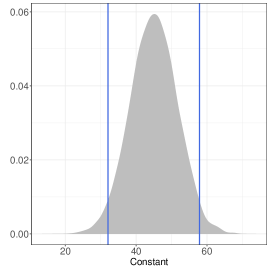
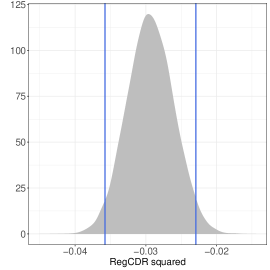
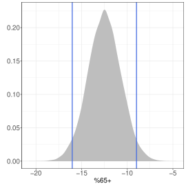
Figure 9. Densities with credible intervals (blue lines). The models are based on an dataset updated to 2019, which uses GBD death estimates based on the GBD 2019 and comprises 120 countries and 2,748 country-years from 1970-2019 [Demographics Collaborators, 2020], both sexes and model 1 using a common Gamma prior for the scale of the errors.

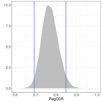
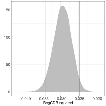
Figure 10. Densities with credible intervals (blue lines). The models are based on an dataset updated to 2019, which uses GBD death estimates based on the GBD 2019 and comprises 120 countries and 2,748 country-years from 1970-2019 [Demographics Collaborators, 2020], both sexes and model 1 using a Half-Cauchy prior for the local scale of the errors.

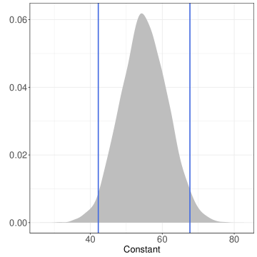
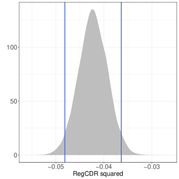
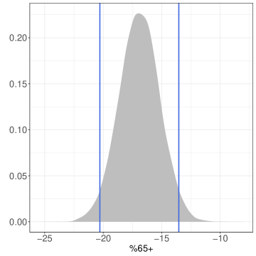
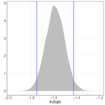
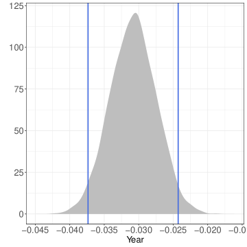
Figure 11. Densities with credible intervals (blue lines). The models are based on an dataset updated to 2019, which uses GBD death estimates based on the GBD 2019 and comprises 120 countries and 2,748 country-years from 1970-2019 [Demographics Collaborators, 2020], both sexes and model 2 using a common Gamma prior for the scale of the errors.

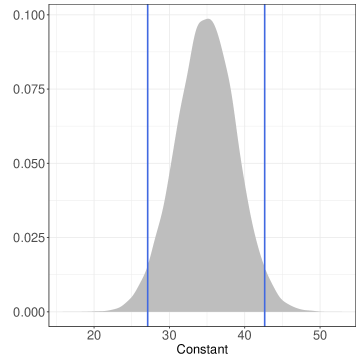
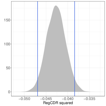
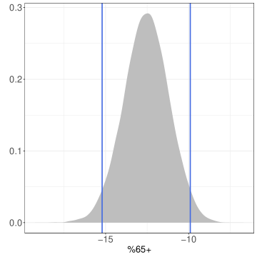
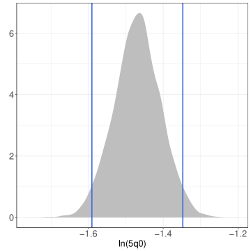
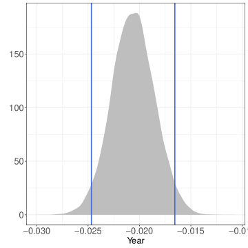
Figure 12. Densities with credible intervals (blue lines). The models are based on an dataset updated to 2019, which uses GBD death estimates based on the GBD 2019 and comprises 120 countries and 2,748 country-years from 1970-2019 [Demographics Collaborators, 2020], both sexes and model 2 using a Half-Cauchy prior for the local scale of the errors.

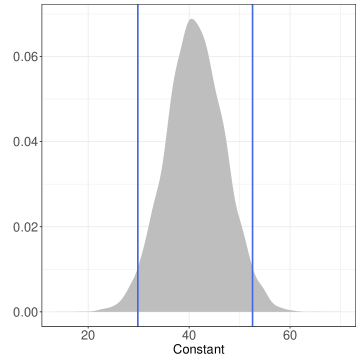
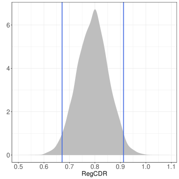
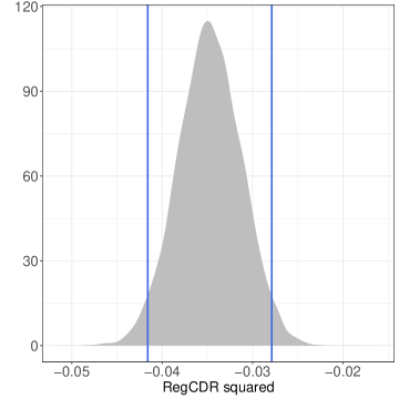
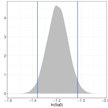
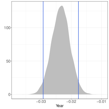
Figure 13. Densities with credible intervals (blue lines). The models are based on an dataset updated to 2019, which uses GBD death estimates based on the GBD 2019 and comprises 120 countries and 2,748 country-years from 1970-2019 [Demographics Collaborators, 2020], females and model 1 using a common Gamma prior for the scale of the errors.

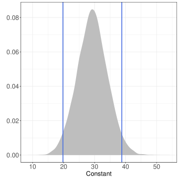
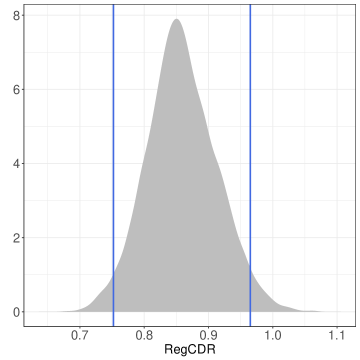
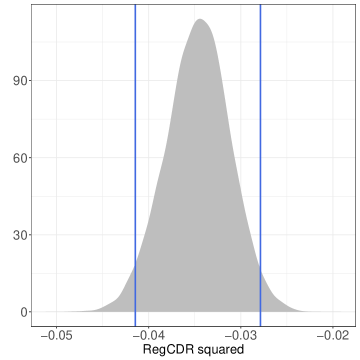
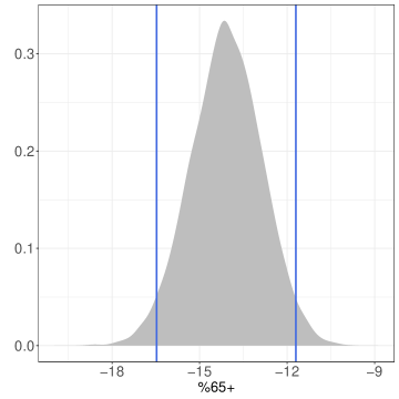
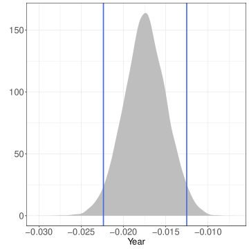
Figure 14. Densities with credible intervals (blue lines). The models are based on an dataset updated to 2019, which uses GBD death estimates based on the GBD 2019 and comprises 120 countries and 2,748 country-years from 1970-2019 [Demographics Collaborators, 2020], females and model 1 using a Half-Cauchy prior for the local scale of the errors.

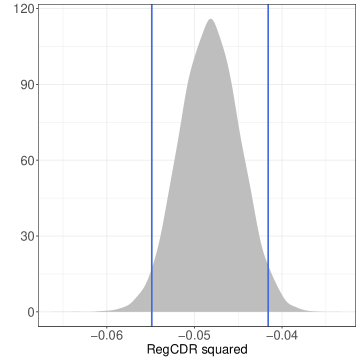
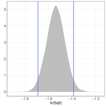
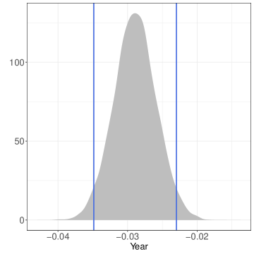
Figure 15. Densities with credible intervals (blue lines). The models are based on an dataset updated to 2019, which uses GBD death estimates based on the GBD 2019 and comprises 120 countries and 2,748 country-years from 1970-2019 [Demographics Collaborators, 2020], females and model 2 using a common Gamma prior for the scale of the errors.

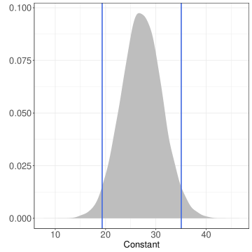
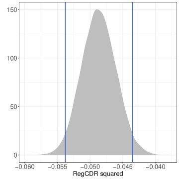
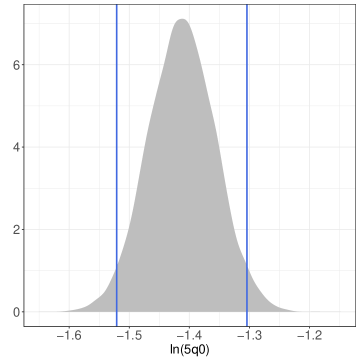
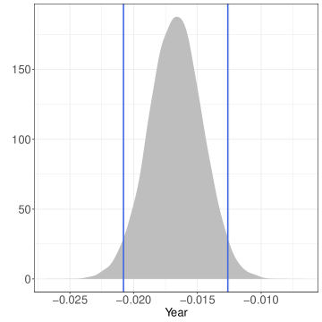
Figure 16. Densities with credible intervals (blue lines). The models are based on an dataset updated to 2019, which uses GBD death estimates based on the GBD 2019 and comprises 120 countries and 2,748 country-years from 1970-2019 [Demographics Collaborators, 2020], females and model 2 using a Half-Cauchy prior for the local scale of the errors

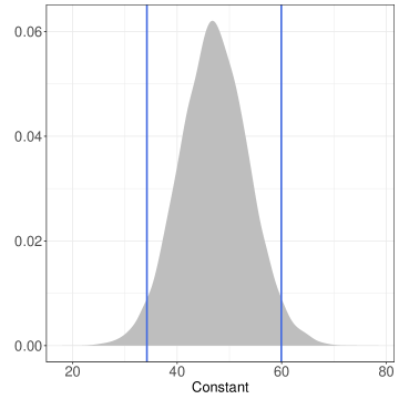
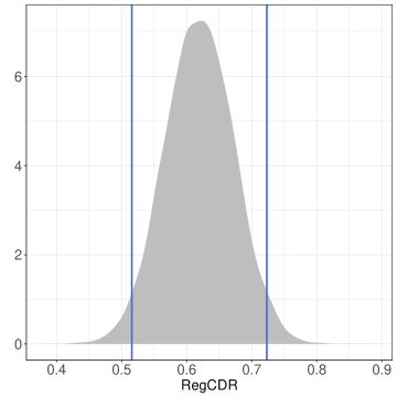
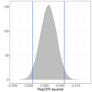
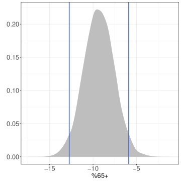
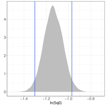
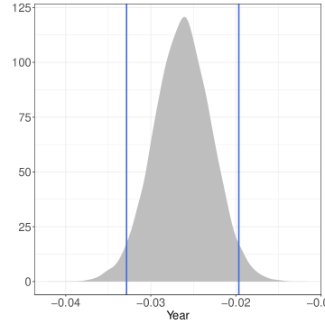
Figure 17. Densities with credible intervals (blue lines). The models are based on an dataset updated to 2019, which uses GBD death estimates based on the GBD 2019 and comprises 120 countries and 2,748 country-years from 1970-2019 [Demographics Collaborators, 2020], males and model 1 using a Half-Cauchy prior for the local scale of the errors.

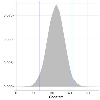
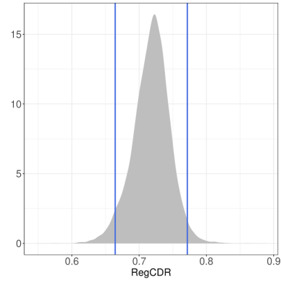
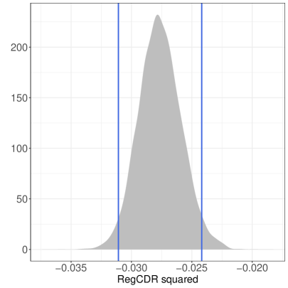
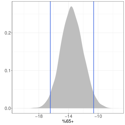
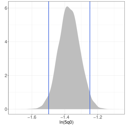
Figure 18. Densities with credible intervals (blue lines). The models are based on an dataset updated to 2019, which uses GBD death estimates based on the GBD 2019 and comprises 120 countries and 2,748 country-years from 1970-2019 [Demographics Collaborators, 2020], males and model 1 using a Half-Cauchy prior for the local scale of the errors.

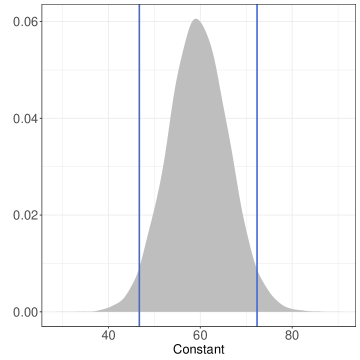
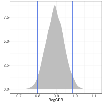
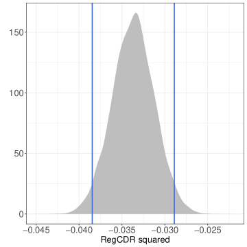
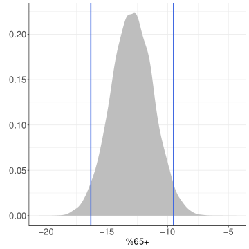
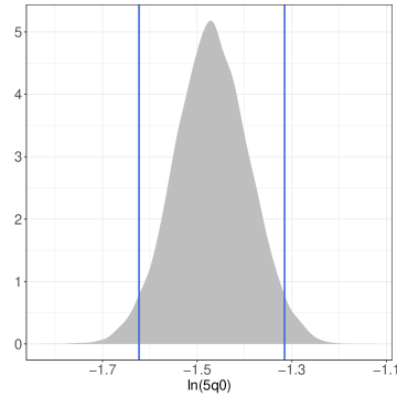
Figure 19. Densities with credible intervals (blue lines). The models are based on an dataset updated to 2019, which uses GBD death estimates based on the GBD 2019 and comprises 120 countries and 2,748 country-years from 1970-2019 [Demographics Collaborators, 2020], males and model 2 using a Half-Cauchy prior for the local scale of the errors.

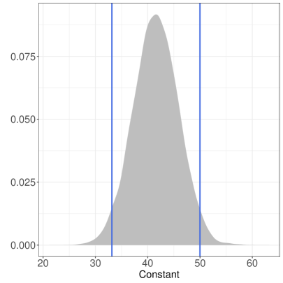
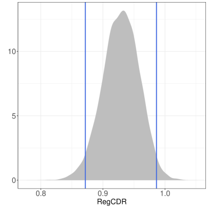
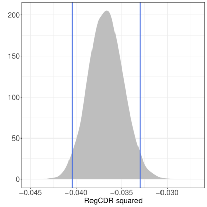
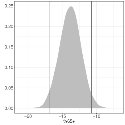
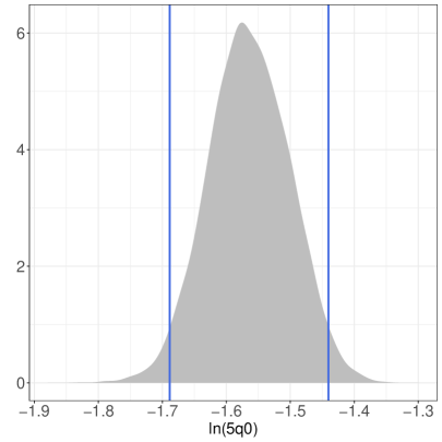
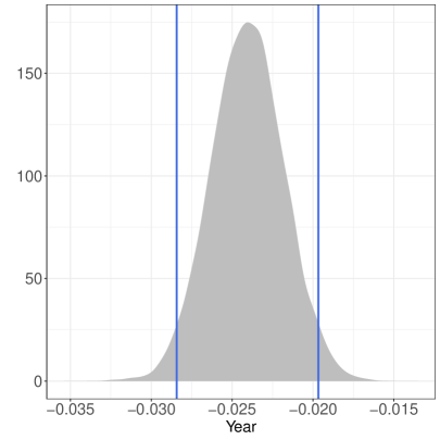
Figure 20. Densities with credible intervals (blue lines). The models are based on an dataset updated to 2019, which uses GBD death estimates based on the GBD 2019 and comprises 120 countries and 2,748 country-years from 1970-2019 [Demographics Collaborators, 2020], males and model 2 using a Half-Cauchy prior for the local scale of the errors

11. Results subnational level

This section contains the posterior predictive estimates at subnational levels (Departments) and national level and the corresponding 95% credible intervals under Gamma, HS, LA and Student-t local scale priors fro the random effects and Half-Cauchy and Gamma global scale priors for the errors. The results for model 1 and 2 for females are presented in Tables 14 and 15 and for males in Tables 16 and 17.

Department	Census	Gamma	$2.5\%$	$97.5\%$	Student-t	$2.5\%$	$97.5\%$	LA	$2.5\%$	$97.5\%$	HS	$2.5\%$	$97.5\%$
Antioquia	94	95	95	96	95	95	96	95	95	96	95	95	96
Atlántico	97	94	93	95	94	93	95	94	93	95	94	93	95
Bogotá, D.C.	97	93	92	94	93	92	94	93	92	94	93	92	94
Bolívar	90	92	91	93	92	91	93	92	91	93	92	90	93
Boyacá	95	94	92	95	94	93	95	94	93	95	94	93	95
Caldas	94	98	97	98	98	97	98	98	97	98	98	97	98
Caquetá	89	93	92	94	93	92	94	93	92	94	93	92	94
Cauca	85	87	85	89	87	85	89	87	85	89	86	84	89
Cesar	89	86	84	88	86	83	88	86	83	88	85	83	88
Córdoba	89	89	86	90	89	86	90	88	86	90	88	86	90
Cundinamarca	94	96	95	97	96	95	97	96	95	97	96	95	97
Chocó	67	67	62	72	67	62	71	67	62	71	65	61	70
Huila	93	92	91	94	92	91	94	92	91	94	92	91	94
La Guajira	38	57	51	62	56	51	62	56	51	61	55	50	60
Magdalena	90	91	89	92	91	89	92	91	89	92	91	89	92
Meta	92	96	96	97	96	96	97	96	96	97	96	95	97
Nariño	85	89	86	90	89	86	90	89	86	90	88	86	90
Norte de Santander	92	93	92	94	93	92	94	93	92	94	93	92	94
Quindio	95	96	95	97	96	95	97	96	95	97	96	95	97
Risaralda	95	97	96	97	97	96	97	97	96	97	97	96	97
Santander	95	93	92	94	93	92	94	93	92	94	93	92	94
Sucre	88	95	94	96	95	94	96	95	94	96	94	93	95
Tolima	93	93	91	94	93	91	94	93	91	94	93	91	94
Valle del Cauca	96	96	95	96	96	95	97	96	95	97	96	95	97
Arauca	86	95	94	96	95	94	96	95	94	96	95	94	96
Casanare	86	95	94	96	95	94	96	95	94	96	95	93	96
Putumayo	82	87	84	89	87	84	89	87	84	89	86	84	88
San Andrés	95	93	92	94	93	92	94	93	91	94	93	91	94
Amazonas	76	68	64	72	68	64	72	68	63	72	67	63	71
Guainía	56	89	85	91	88	85	91	88	85	91	87	84	90
Guaviare	79	93	91	94	93	91	94	93	91	94	92	90	94
Vaupés	62	63	58	68	63	58	68	63	58	67	61	57	67
Vichada	62	88	84	90	87	84	90	87	84	90	86	82	89
National	92	93	91	94	93	91	94	93	91	94	93	91	94

Table 14. Posterior predictive estimates and 95% credible intervals under Gamma, HS, LA and Student-t local priors for the random effects and Half-Cauchy local prior for the errors and census based completeness values. Inf and Sup represent the 2.5% and 97.5% quantiles from the posterior marginal distribution of the completeness in each Department and at the national level. Females and model 1.

Department	Census	Gamma	$2.5\%$	$97.5\%$	Student-t	$2.5\%$	$97.5\%$	LA	$2.5\%$	$97.5\%$	HS	$2.5\%$	$97.5\%$
Antioquia	94	95	94	96	95	94	96	95	94	96	95	94	96
Atlántico	97	94	93	95	94	93	95	94	93	95	94	92	95
Bogotá, D.C.	97	93	92	94	93	92	94	93	92	94	93	91	94
Bolívar	90	91	89	92	91	89	92	91	89	92	91	89	92
Boyacá	95	94	93	95	94	93	95	94	93	95	94	93	95
Caldas	94	98	97	98	98	97	98	98	97	98	98	97	98
Caquetá	89	92	91	93	92	91	93	92	91	93	92	90	93
Cauca	85	85	83	88	85	83	88	85	83	88	85	82	88
Cesar	89	83	81	86	83	81	86	83	81	86	83	80	86
Córdoba	89	87	84	89	87	85	89	87	84	89	87	84	89
Cundinamarca	94	95	94	96	95	95	96	95	94	96	95	94	96
Chocó	67	60	56	65	60	56	65	60	55	65	60	55	65
Huila	93	93	92	94	93	92	94	93	92	94	93	92	94
La Guajira	38	53	48	58	53	47	58	52	47	57	52	47	57
Magdalena	90	89	87	91	89	87	91	89	87	91	89	87	91
Meta	92	95	94	96	95	94	96	95	94	96	95	94	96
Nariño	85	89	87	91	89	87	91	89	87	91	89	86	91
Norte de Santander	92	93	92	94	94	92	95	93	92	94	93	92	94
Quindio	95	96	95	97	96	95	97	96	95	97	96	95	97
Risaralda	95	97	96	97	97	96	97	97	96	97	97	96	97
Santander	95	94	93	95	94	93	95	94	93	95	94	92	95
Sucre	88	93	92	94	93	92	94	93	92	94	93	92	94
Tolima	93	94	93	95	94	93	95	94	93	95	94	93	95
Valle del Cauca	96	96	95	97	96	95	97	96	95	97	96	95	97
Arauca	86	94	93	95	94	93	95	94	93	95	94	93	95
Casanare	86	92	91	94	92	91	94	92	91	94	92	91	93
Putumayo	82	87	85	89	87	85	89	87	85	89	87	85	89
San Andrés	95	90	88	91	90	88	91	90	88	91	90	88	91
Amazonas	76	66	62	70	66	62	70	66	62	70	66	61	70
Guainía	56	80	77	83	80	77	83	80	77	83	80	77	83
Guaviare	79	89	87	90	89	87	90	89	87	90	89	86	90
Vaupés	62	58	53	62	58	53	62	57	53	62	57	52	62
Vichada	62	78	75	81	78	74	81	78	74	81	78	74	81
National	92	92	91	94	93	91	94	93	91	94	93	91	94

Table 15. Posterior predictive estimates and 95% credible intervals under Gamma, HS, LA and Student-t local priors for the random effects and a Half-Cauchy local prior for the errors and census based completeness values. Inf and Sup represent the 2.5% and 97.5% quantiles from the posterior marginal distribution of the completeness in each Department and at the national level. Females and model 2.

Department	Census	Gamma	$2.5\%$	$97.5\%$	Student-t	$2.5\%$	$97.5\%$	LA	$2.5\%$	$97.5\%$	HS	$2.5\%$	$97.5\%$
Antioquia	92	94	94	95	94	94	95	94	94	95	95	94	95
Atlántico	95	93	92	94	93	92	94	93	92	94	93	92	94
Bogotá, D.C.	95	91	90	93	91	90	93	91	90	93	92	90	93
Bolívar	87	89	87	90	89	87	90	89	87	90	89	87	90
Boyacá	92	92	90	93	92	90	93	92	90	93	92	91	93
Caldas	92	97	97	98	97	97	98	97	97	98	98	97	98
Caquetá	87	93	92	94	93	92	94	93	92	94	93	92	94
Cauca	81	80	76	82	79	76	82	79	76	82	79	76	82
Cesar	87	82	79	85	82	79	84	82	79	84	81	79	83
Córdoba	87	85	82	87	85	82	87	85	82	87	85	82	87
Cundinamarca	93	95	94	96	95	94	96	95	94	96	96	95	96
Chocó	64	58	53	63	57	53	62	57	52	62	55	51	59
Huila	92	89	88	91	89	88	91	89	88	91	89	88	91
La Guajira	40	50	45	55	49	44	54	48	43	53	46	41	50
Magdalena	86	89	87	90	89	87	90	88	87	90	89	87	90
Meta	90	95	95	96	95	95	96	95	95	96	96	95	96
Nariño	79	82	79	84	82	79	84	82	79	84	82	79	84
Norte de Santander	90	92	91	93	92	91	93	92	91	93	92	91	93
Quindio	94	95	94	96	95	94	96	95	94	96	96	95	97
Risaralda	92	96	96	97	96	96	97	96	96	97	97	96	97
Santander	93	91	90	92	91	90	92	91	90	92	91	90	92
Sucre	85	92	91	93	92	91	93	92	91	93	92	91	94
Tolima	90	89	87	91	89	87	91	89	87	91	90	88	91
Valle del Cauca	94	96	95	97	96	95	97	96	95	97	96	96	97
Arauca	85	96	96	97	96	96	97	96	96	97	96	96	97
Casanare	87	93	91	94	93	91	94	93	91	94	93	92	94
Putumayo	76	81	79	84	81	78	84	81	78	83	80	77	82
San Andrés	92	96	96	97	96	96	97	96	96	97	96	96	97
Amazonas	62	72	68	76	72	68	75	71	67	75	70	66	73
Guainía	49	84	82	87	84	81	86	84	81	86	84	81	86
Guaviare	82	94	93	95	94	93	95	94	93	95	94	93	95
Vaupés	54	57	52	62	56	51	61	55	51	60	53	49	57
Vichada	59	80	77	83	79	76	82	79	76	82	79	76	82
National	89	91	90	92	91	90	92	91	90	92	91	90	92

Table 16. Posterior predictive estimates and 95% credible intervals under Gamma, HS, LA and Student-t local priors for the random effects and a Half-Cauchy local prior for the scale of the errors and the observed estimates from the census. Inf and Sup represent the 2.5% and 97.5% quantiles from the marginal posterior distribution of the completeness in each Department and at the national level. Males and model 1.

Department	Census	Gamma	$2.5\%$	$97.5\%$	Student-t	$2.5\%$	$97.5\%$	LA	$2.5\%$	$97.5\%$	HS	$2.5\%$	$97.5\%$
Antioquia	92	94	93	95	94	93	95	94	93	95	94	93	95
Atlántico	95	90	89	92	90	89	92	90	89	92	91	89	92
Bogotá, D.C.	95	89	87	90	89	87	90	89	87	90	89	88	90
Bolívar	87	85	83	87	85	83	87	85	83	87	85	83	87
Boyacá	92	91	90	93	91	90	93	91	90	93	92	90	93
Caldas	92	97	96	97	97	96	97	97	96	98	97	97	98
Caquetá	87	92	91	93	92	91	93	92	91	93	92	91	93
Cauca	81	77	73	80	77	73	80	77	73	80	77	73	80
Cesar	87	77	74	80	77	74	79	77	74	79	77	74	79
Córdoba	87	78	75	81	78	75	81	78	75	81	79	76	82
Cundinamarca	93	93	92	94	93	92	94	93	93	94	94	93	95
Chocó	64	47	42	52	47	42	51	46	42	51	46	41	51
Huila	92	90	88	91	90	88	91	90	88	91	90	88	91
La Guajira	40	41	36	45	40	36	45	40	35	44	39	35	44
Magdalena	86	84	82	86	84	82	86	84	82	86	84	82	86
Meta	90	94	93	95	94	93	95	94	93	95	94	94	95
Nariño	79	82	79	84	82	79	84	82	79	84	82	79	85
Norte de Santander	90	92	91	93	92	91	93	92	91	93	92	91	93
Quindio	94	95	94	96	95	94	96	95	94	96	96	95	97
Risaralda	92	96	95	96	96	95	96	96	95	96	96	95	97
Santander	93	92	90	93	92	91	93	92	91	93	92	91	93
Sucre	85	88	86	90	88	87	90	88	87	90	89	87	90
Tolima	90	90	88	92	91	89	92	91	89	92	91	89	93
Valle del Cauca	94	96	95	96	96	95	96	96	95	96	96	95	97
Arauca	85	95	94	95	95	94	95	95	94	95	95	94	96
Casanare	87	90	89	92	90	89	92	90	89	92	91	89	92
Putumayo	76	77	74	80	77	74	79	77	74	79	77	74	79
San Andrés	92	95	95	96	95	95	96	95	95	96	95	95	96
Amazonas	62	60	56	64	60	56	64	60	56	64	59	56	63
Guainía	49	72	68	75	72	68	75	72	68	75	71	68	75
Guaviare	82	93	92	94	93	92	94	93	92	94	93	92	94
Vaupés	54	53	49	58	53	48	57	52	48	57	52	47	56
Vichada	59	69	66	73	69	65	73	69	65	73	69	65	73
National	89	89	88	91	89	88	91	89	88	91	90	88	91

Table 17. Posterior predictive estimates and 95% credible intervals under Gamma, HS, LA and Student-t local priors for the random effects and a Half-Cauchy local prior for the scale of the errors and the observed estimates from the census. Inf and Sup represent the 2.5% and 97.5% quantiles from the marginal posterior distribution of the completeness in each Department and at the national level. Males and model 2.

References

- Adair and Lopez [2018] Tim Adair and Alan D Lopez. Estimating the completeness of death registration: An empirical method. PloS one, 13(5):e0197047, 2018.
- Adair et al. [2021] Tim Adair, Sonja Firth, Tint Pa Pa Phyo, Khin Sandar Bo, and Alan D Lopez. Monitoring progress with national and subnational health goals by integrating verbal autopsy and medically certified cause of death data. BMJ global health, 6(5):e005387, 2021.
- Alkema et al. [2017] Leontine Alkema, Sanqian Zhang, Doris Chou, Alison Gemmill, Ann-Beth Moller, Doris Ma Fat, Lale Say, Colin Mathers, and Daniel Hogan. A bayesian approach to the global estimation of maternal mortality. The Annals of Applied Statistics, 11(3):1245–1274, 2017.
- Armagan et al. [2013] Artin Armagan, David B Dunson, and Jaeyong Lee. Generalized double pareto shrinkage. Statistica Sinica, 23(1):119, 2013.
- Azose and Raftery [2015] Jonathan J Azose and Adrian E Raftery. Bayesian probabilistic projection of international migration. Demography, 52(5):1627–1650, 2015.
- Bai and Ghosh [2018] Ray Bai and Malay Ghosh. High-dimensional multivariate posterior consistency under global–local shrinkage priors. Journal of Multivariate Analysis, 167:157–170, 2018.
- Basu and Adair [2021] Jayanta Kumar Basu and Tim Adair. Have inequalities in completeness of death registration between states in india narrowed during two decades of civil registration system strengthening? International journal for equity in health, 20(1):1–9, 2021.
- Bennett and Horiuchi [1984] Neil G Bennett and Shiro Horiuchi. Mortality estimation from registered deaths in less developed countries. Demography, 21(2):217–233, 1984.
- Bhadra et al. [2017] Anindya Bhadra, Jyotishka Datta, Nicholas G Polson, and Brandon Willard. The horseshoe+ estimator of ultra-sparse signals. Bayesian Analysis, 12(4):1105–1131, 2017.
- Bhattacharya et al. [2015] Anirban Bhattacharya, Debdeep Pati, Natesh S Pillai, and David B Dunson. Dirichlet–laplace priors for optimal shrinkage. Journal of the American Statistical Association, 110(512):1479–1490, 2015.
- Brass et al. [1975] William Brass et al. Methods for estimating fertility and mortality from limited and defective data. Methods for estimating fertility and mortality from limited and defective data., 1975.
- Brown and Griffin [2010] Philip J Brown and Jim E Griffin. Inference with normal-gamma prior distributions in regression problems. Bayesian analysis, 5(1):171–188, 2010.
- Carvalho et al. [2010] Carlos M Carvalho, Nicholas G Polson, and James G Scott. The horseshoe estimator for sparse signals. Biometrika, 97(2):465–480, 2010.
- DANE [2017a] DANE. Defunciones no fetales 2017. Technical report, Departamento Administrativo Nacional de Estadística, 2017a.
- DANE [2017b] DANE. Proyecciones de población. Technical report, Departamento Administrativo Nacional de Estadística, 2017b.
- DANE [2018] DANE. Censo nacional de población y vivienda - cnpv - 2018. Technical report, Departamento Administrativo Nacional de Estadística, 2018.
- Demographics Collaborators [2020] GBD 2019 Demographics Collaborators. Global age-sex-specific fertility, mortality, healthy life expectancy (hale), and population estimates in 204 countries and territories, 1950–2019: a comprehensive demographic analysis for the global burden of disease study 2019. The Lancet, 396(10258):1160–1203, 2020.
- DHS [2010] DHS. Encuesta nacional de demografía y salud – ends 2011. profamilia. Technical report, 2010.
- DHS [2015] DHS. Encuesta nacional de demografía y salud – ends 2015. profamilia. Technical report, 2015.
- Dicker et al. [2018] Daniel Dicker, Grant Nguyen, Degu Abate, Kalkidan Hassen Abate, Solomon M Abay, Cristiana Abbafati, Nooshin Abbasi, Hedayat Abbastabar, Foad Abd-Allah, Jemal Abdela, et al. Global, regional, and national age-sex-specific mortality and life expectancy, 1950–2017: a systematic analysis for the global burden of disease study 2017. The lancet, 392(10159):1684–1735, 2018.
- Dorrington [2013a] R Dorrington. The brass growth balance method. Tools for demographic estimation. Paris: IUSSP, pages 196–208, 2013a.
- Dorrington [2013b] R Dorrington. The generalized growth balance method. Tools for demographic estimation, pages 258–274, 2013b.
- Dorrington [2013c] Rob Dorrington. Synthetic extinct generations methods. Tools for demographic estimation, pages 275–292, 2013c.
- Frühwirth-Schnatter and Wagner [2011] S Frühwirth-Schnatter and H Wagner. Bayesian variable selection for random intercept modeling of gaussian and non-gaussian data. Bayesian statistics, 9:165–185, 2011.
- Gelfand and Smith [1990] Alan E Gelfand and Adrian FM Smith. Sampling-based approaches to calculating marginal densities. Journal of the American statistical association, 85(410):398–409, 1990.
- Ghosh et al. [2016] Prasenjit Ghosh, Xueying Tang, Malay Ghosh, and Arijit Chakrabarti. Asymptotic properties of bayes risk of a general class of shrinkage priors in multiple hypothesis testing under sparsity. Bayesian Analysis, 11(3):753–796, 2016.
- Godwin and Raftery [2017] Jessica Godwin and Adrian E Raftery. Bayesian projection of life expectancy accounting for the hiv/aids epidemic. Demographic research, 37:1549, 2017.
- Griffin and Brown [2005] JE Griffin and PJ Brown. Alternative prior distributions for variable selection with very many more variables than observations. Technical report, Technical report, University of Warwick, 2005.
- Hill [1987] Kenneth Hill. Estimating census and death registration completeness. In Asian and Pacific population forum/East-West Population Institute, East-West Center, volume 1, pages 8–13. The Asian & Pacific Population Forum, 1987.
- Juárez and Steel [2010] Miguel A Juárez and Mark FJ Steel. Model-based clustering of non-gaussian panel data based on skew-t distributions. Journal of Business & Economic Statistics, 28(1):52–66, 2010.
- Mikkelsen et al. [2015] Lene Mikkelsen, David E Phillips, Carla AbouZahr, Philip W Setel, Don De Savigny, Rafael Lozano, and Alan D L opez. A global assessment of civil registration and vital statistics systems: monitoring data quality and progress. The Lancet, 386(10001):1395–1406, 2015.
- Murray et al. [2010] Christopher JL Murray, Julie Knoll Rajaratnam, Jacob Marcus, Thomas Laakso, and Alan D Lopez. What can we conclude from death registration? improved methods for evaluating completeness. PLoS medicine, 7(4):e1000262, 2010.
- Polson and Scott [2012] Nicholas G Polson and James G Scott. On the half-cauchy prior for a global scale parameter. Bayesian Analysis, 7(4):887–902, 2012.
- Preston et al. [1980] Samuel Preston, Ansley J Coale, James Trussell, and Maxine Weinstein. Estimating the completeness of reporting of adult deaths in populations that are approximately stable. Population index, pages 179–202, 1980.
- Raftery et al. [2014] Adrian E Raftery, Leontine Alkema, and Patrick Gerland. Bayesian population projections for the united nations. Statistical science: a review journal of the Institute of Mathematical Statistics, 29(1):58, 2014.
- Rao and Kelly [2017] C Rao and M Kelly. Overview of the principles and international experiences in implementing record linkage mechanisms to assess completeness of death registration. Population Division, Department of Economic and Social Affairs, United Nations, New York, (2017/5), 2017.
- Rossell and Steel [2019] David Rossell and Mark FJ Steel. Continuous mixtures with skewness and heavy tails. In Handbook of Mixture Analysis, pages 219–237. Chapman and Hall/CRC, 2019.
- Rubio and Steel [2015] FJ Rubio and MFJ Steel. Bayesian modelling of skewness and kurtosis with two-piece scale and shape distributions. Electronic Journal of Statistics, 9(2):1884–1912, 2015.
- Sempé et al. [2021] Lucas Sempé, Peter Lloyd-Sherlock, Ramón Martínez, Shah Ebrahim, Martin McKee, and Enrique Acosta. Estimation of all-cause excess mortality by age-specific mortality patterns for countries with incomplete vital statistics: a population-based study of the case of peru during the first wave of the covid-19 pandemic. The Lancet Regional Health-Americas, 2:100039, 2021.
- Shawon et al. [2021] Md Toufiq Hassan Shawon, Shah Ali Akbar Ashrafi, Abul Kalam Azad, Sonja M Firth, Hafizur Chowdhury, Robert G Mswia, Tim Adair, Ian Riley, Carla Abouzahr, and Alan D Lopez. Routine mortality surveillance to identify the cause of death pattern for out-of-hospital adult (aged 12+ years) deaths in bangladesh: introduction of automated verbal autopsy. BMC public health, 21(1):1–11, 2021.
- Tang et al. [2018a] Xueying Tang, Malay Ghosh, Neung Soo Ha, and Joseph Sedransk. Modeling random effects using global–local shrinkage priors in small area estimation. Journal of the American Statistical Association, 113(524):1476–1489, 2018a.
- Tang et al. [2018b] Xueying Tang, Xiaofan Xu, Malay Ghosh, and Prasenjit Ghosh. Bayesian variable selection and estimation based on global-local shrinkage priors. Sankhya A, 80(2):215–246, 2018b.
- UN [2019] UN. New york: United nations department of economic and social affairs. Population Division. World Population Prospects: The 2019 Revision, 2019.
- Villa and Walker [2014] Cristiano Villa and Stephen G Walker. Objective prior for the number of degrees of freedom of at distribution. Bayesian Analysis, 9(1):197–220, 2014.
- Wang et al. [2014] Haidong Wang, Chelsea A Liddell, Matthew M Coates, Meghan D Mooney, Carly E Levitz, Austin E Schumacher, Henry Apfel, Marissa Iannarone, Bryan Phillips, Katherine T Lofgren, et al. Global, regional, and national levels of neonatal, infant, and under-5 mortality during 1990–2013: a systematic analysis for the global burden of disease study 2013. The Lancet, 384(9947):957–979, 2014.
- Wang et al. [2020] Haidong Wang, Kaja M Abbas, Mitra Abbasifard, Mohsen Abbasi-Kangevari, Hedayat Abbastabar, Foad Abd-Allah, Ahmed Abdelalim, Hassan Abolhassani, Lucas Guimarães Abreu, Michael RM Abrigo, et al. Global age-sex-specific fertility, mortality, healthy life expectancy (hale), and population estimates in 204 countries and territories, 1950–2019: a comprehensive demographic analysis for the global burden of disease study 2019. The Lancet, 396(10258):1160–1203, 2020.
- Wheldon et al. [2016] Mark C Wheldon, Adrian E Raftery, Samuel J Clark, and Patrick Gerland. Bayesian population reconstruction of female populations for less developed and more developed countries. Population studies, 70(1):21–37, 2016.
- Zeng et al. [2020] Xinying Zeng, Tim Adair, Lijun Wang, Peng Yin, Jinlei Qi, Yunning Liu, Jiangmei Liu, Alan D Lopez, and Maigeng Zhou. Measuring the completeness of death registration in 2844 chinese counties in 2018. BMC medicine, 18(1):1–11, 2020.