On Squared-Variable Formulations

Abstract

We revisit a formulation technique for inequality constrained optimization problems that has been known for decades: the substitution of squared variables for nonnegative variables. Using this technique, inequality constraints are converted to equality constraints via the introduction of a squared-slack variable. Such formulations have the superficial advantage that inequality constraints can be dispensed with altogether. But there are clear disadvantages, not least being that first-order optimal points for the squared-variable reformulation may not correspond to first-order optimal points for the original problem, because the Lagrange multipliers may have the wrong sign. Extending previous results, this paper shows that points satisfying approximate second-order optimality conditions for the squared-variable reformulation also, under certain conditions, satisfy approximate second-order optimality conditions for the original formulation, and vice versa. Such results allow us to adapt complexity analysis of methods for equality constrained optimization to account for inequality constraints. On the algorithmic side, we examine squared-variable formulations for several interesting problem classes, including bound-constrained quadratic programming and linear programming. We show that algorithms built on these formulations are surprisingly competitive with standard methods. For linear programming, we examine the relationship between the squared-variable approach and primal-dual interior-point methods.

1 Introduction

Consider a smooth objective $f:^{n}\rightarrow$ and smooth vector function $c:^{n}\rightarrow^{m}$ that define an inequality constrained optimization problem

(NLP) $$\min_{x}\,f(x)\;\;\mbox{s.t.}\;\;c(x)\geq 0.$$

A formulation of this problem using squared-slack variables (SSV) is

(SSV) $$\min_{x,v}\,f(x)\;\;\mbox{s.t.}\;\;c(x)-v\odot v=0,$$

where $v\in\mathbb{R}^{m}$. Relatedly, we can use squared variables in place of nonnegative variables. Consider the problem

(BC) $$\min_{x}\,f(x)\;\;\mbox{s.t.}\;\;x\geq 0.$$

By directly substituting $x=v\odot v$, we obtain the unconstrained problem

(DSS) $$\min_{v}\,F(v):=f(v\odot v).$$

Squared-slack variables have a long history in optimization as a means of converting a problem with inequality constraints into one with equality constraints, thereby avoiding the issues involved in determining which inequality constraints are active at the solution. Despite this superficial appeal, there are potentially serious objections to the approach, including the following.

1. A first-order optimal point for (SSV) may not yield a first-order point for (NLP), because Lagrange multipliers for the constraints in (SSV) may have either sign, whereas Lagrange multipliers in (NLP) must be nonnegative.

2. Any solution $x^{*}$ of (NLP) corresponds to a multiplicity of solutions of (SSV), obtained by setting $v_{i}^{*}=\pm\sqrt{c_{i}(x^{*})}$. That is, the sign of $v_{i}$ is not well defined.

3. Convexity of the original formulation is generally lost in the squared-variable formulations.

4. The reformulated problem is “more nonlinear.” Linear inequality constraints become quadratic equality constraints, quadratic objectives may become quartic, and so on.

5. Certain issues involving conditioning and numerical stability (that depend on the choice of algorithm) arise in (SSV) that do not appear in (NLP).

Early papers of Tapia [11, 12] described Newton and quasi-Newton methods applied to the first-order optimality conditions for (SSV), but while mentioning the issue concerning the sign of the Lagrange multipliers, did not propose a strategy to address it. Bertsekas [1, Section 3.3.2] uses the squared-slack formulation for theoretical purposes, in deriving optimality conditions for inequality-constrained optimization. He shows that when the primal-dual solution $(x^{*},v^{*},s^{*})$ of (SSV) ($s^{*}$ being the Lagrange multiplier for the equality constraint) satisfies second-order necessary conditions with $v^{*}\geq 0$, then $(x^{*},s^{*})$ satisfies the first- and a weak form of second-order necessary conditions for (NLP). (In fact, it is trivial to drop the restriction $v^{*}\geq 0$.) Fukuda and Fukushima [3] show that when the primal-dual solution $(x^{*},v^{*},s^{*})$ of (SSV) satisfies second-order sufficient conditions, then $(x^{*},s^{*})$ satisfies second-order sufficient conditions for (NLP). They also discuss the relationship between LICQ in the two formulations.

The direct-square-substitution approach (DSS) for the bound-constrained problem (BC) is discussed in Gill, Murray, and Wright’s text [5, pp. 268-269]. They point out (as we discuss in Section 2) that spurious saddle points for the reformulated problem arise when some components of $v$ are zero.

The paper [8] considers optimization over the simplex, in which the constraint $\mathbf{1}_{n}^{T}x=1$ is added to the nonnegativity constraints in (BC). The paper explores the reformulation (DSS), with the constraint $\sum_{i=1}^{n}v_{i}^{2}=1$ included, and treats the resulting problem as one of minimization over the Riemannian manifold $\mathcal{S}_{n-1}:=\{v\,|\,\sum_{i=1}^{n}v_{i}^{2}=1\}$, referring to this reformulation technique as the “Hadamard parametrization.” They apply a perturbed form of Riemannian gradient descent to this formulation, with various steplength selection strategies, proving convergence to a second-order optimal point of the original problem, with a certain complexity guarantee $\mathcal{O}(\log^{4}n/\epsilon)$ (under assumptions of a strict saddle property, nondegeneracy, and no spurious local minima.) In [7], settings beyond the simplex constraint are considered, such as the set of low-rank matrices, and show landscape results concerning exact first and second-order necessary points.

Motivation, Outline, Contributions

In the paper we examine several aspects of squared-variable formulations. First, we examine points that satisfy second-order optimality conditions approximately for the direct-square-substitution and squared-slack formulations, and discuss whether such points satisfy approximate second-order optimality conditions for the original formulations. This connection allows us to perform a complexity analysis for the inequality-constrained problem (NLP) by applying recent results on complexity of equality-constrained optimization to the formulation (SSV). Second, we focus on a squared-variable formulation of linear programming, and draw connections between sequential quadratic programming applied to this formulation and the classical primal-dual interior-point method. In a final section, we report preliminary numerical results for several formulations of interest, including bound-constrained convex quadratic programming, least-squares problem with “pseudo-norm” constraints (a problem class that arises in variable selection in linear statistical models and compressed sensing), and linear programming.

Notation

The Hadamard product $\odot$ of two vectors $v$ and $w$ of identical length is defined as $v\odot w=[v_{i}w_{i}]_{i=1}^{n}$. In particular, $v\odot v=[v_{i}^{2}]_{i=1}^{n}$. We use $\mathbf{1}_{n}$ to be the vector in $\mathbb{R}^{n}$ whose components are all $1$. For a vector $v\in\mathbb{R}^{n}$, $\operatorname{diag}(v)$ is the $n\times n$ diagonal matrix whose $i$th diagonal element is $v_{i}$, $i=1,2,\dotsc,n$. We often abbreviate the term “second-order necessary” by “2N”. A “2N point” is a point that satisfies second-order necessary conditions. We occasionally use “1N” for first-order necessary conditions.

2 Nonnegativity constraints

Here we discuss the relationship between optimality conditions for the original formulation and squared-variable reformulation of problems in which the variables are constrained to be nonnegative.

Consider the bound-constrained problem (BC) and its reformulation (DSS). Using the notation $V=\operatorname{diag}(v)$, the gradients and Hessian of $F$ are, respectively,

(1a) $$\nabla F(v) =2V\nabla f(v\odot v),$$

(1b) $$\nabla^{2}F(v) =2\operatorname{diag}(\nabla f(v\odot v))+4V\nabla^{2}f(v\odot v)V.$$

Optimality conditions for (BC) are as follows.

Definition 2.1.

We say that $x^{*}$ satisfies first-order conditions to be a solution of (BC) if $0\leq x^{*}\perp\nabla f(x^{*})\geq 0$. We say that strict complementarity is satisfied at $x^{*}$ if $x^{*}$ satisfies first-order conditons and either $x^{*}_{i}>0$ or $[\nabla f(x^{*})]_{i}>0$ for each $i=1,2,\dotsc,n$. We say that $x^{*}$ satisfies weak second-order necessary conditions to be a solution of (BC) if it satisfies first-order conditions and in addition $w^{T}\nabla^{2}f(x^{*})w\geq 0$ for all $w$ such that $x^{*}_{i}=0\Rightarrow w_{i}=0$. We say that $x^{*}$ satisfies second-order sufficient conditions to be a solution of (BC) if it satisfies first-order conditions and in addition $w^{T}\nabla^{2}f(x^{*})w>0$ for all $w\neq 0$ such that $x^{*}_{i}=0,[\nabla f(x^{*})]_{i}>0\Rightarrow w_{i}=0$ and $x^{*}_{i}=0,[\nabla f(x^{*})]_{i}=0\Rightarrow w_{i}\geq 0$.

The second-order necessary conditions of this definition require a copositivity condition to be satisfied in general, which is hard to check, whereas the weak second-order necessary conditions require positive semidefiniteness to be satisfied on a subspace of $\mathbb{R}^{n}$, which is easy to check. The two kinds of conditions differ when there is degeneracy, in the sense that $x^{*}_{i}=[\nabla f(x^{*})]_{i}=0$ for some $i$.

We turn next to optimality conditions for (DSS). The following definition is standard.

Definition 2.2.

We say that $v^{*}$ satisfies first-order necessary conditions to be a solution of (DSS) when $\nabla F(v^{*})=0$. We say that $v^{*}$ satisfies second-order necessary conditions to be a solution of (DSS) if $\nabla F(v^{*})=0$ and $\nabla^{2}F(v^{*})\succeq 0$. We say that $v^{*}$ satisfies second-order sufficient conditions to be a solution of (DSS) if $\nabla F(v^{*})=0$ and $\nabla^{2}F(v^{*})\succ 0$.

The following result relates second-order necessary conditions for the two formulations (BC) and (DSS).

Theorem 2.3.

$x^{*}$ satisfies weak second-order conditions for (BC) if and only if $v^{*}$ defined by $v^{*}_{i}=\pm\sqrt{x^{*}_{i}}$ satisfies second-order necessary conditions for (DSS).

Proof 2.4.

Suppose that $x^{*}$ satisfies weak second-order conditions for (BC), and define $v^{*}$ as in the theorem. Since $x^{*}_{i}\neq 0\iff v^{*}_{i}\neq 0$, the complementarity conditions imply that $\nabla F(v^{*})=V^{*}\nabla f(v^{*}\odot v^{*})=0$, where $V^{*}:=\operatorname{diag}(v^{*})$. Given any $s\in\mathbb{R}^{n}$, we have

(2) $$s^{T}\nabla^{2}F(v^{*})s =2\sum_{i=1}^{n}s_{i}^{2}[\nabla f(x^{*})]_{i}+4(Vs)^{T}\nabla^{2}f(x^{*})(Vs)$$

$$=2\sum_{i=1}^{n}s_{i}^{2}[\nabla f(x^{*})]_{i}+4\sum_{i:x^{*}_{i}\neq 0}\sum_{j:x^{*}_{j}\neq 0}[\nabla^{2}f(x^{*})]_{ij}(Vs)_{i}(Vs)_{j}\geq 0,$$

since $\nabla f(x^{*})\geq 0$ and the weak second-order conditions hold for (BC) at $x^{*}$. Thus second-order necessary conditions hold for (DSS) hold at $v^{*}$.

Suppose now that second-order necessary conditions hold for (DSS) hold at $v^{*}$, and set $x^{*}=v^{*}\odot v^{*}$. We have $x^{*}\geq 0$ and that the complementarity condition $x^{*}\perp\nabla f(x^{*})$ holds because $0=\nabla F(x^{*})=V^{*}\nabla f(x^{*})=X^{*}\nabla f(x^{*})$. Choosing any $s\in\mathbb{R}^{n}$, we have from (1b) that

(3) $$0\leq s^{T}\nabla^{2}F(v^{*})s=2\sum_{i:x^{*}_{i}=0}s_{i}^{2}[\nabla f(x^{*})]_{i}+4\sum_{i:x^{*}_{i}\neq 0}\sum_{j:x^{*}_{j}\neq 0}(V^{*}s)_{i}(V^{*}s)_{j}[\nabla^{2}f(v^{*})]_{ij}.$$

By choosing $s=e_{i}$ for any $i$ with $x^{*}_{i}=0$ we have $0\leq[\nabla f(x^{*})]_{i}$ which implies that the first summation in (3) is nonnegative for any $s$. Given any $w$ with $x^{*}_{i}=0\Rightarrow w_{i}=0$, we have from (3), by setting $s_{i}=w_{i}/v^{*}_{i}$ for $i:x^{*}_{i}\neq 0$ and $s_{i}=0$ otherwise, that $0\leq w^{T}\nabla^{2}f(x^{*})w$, so weak second-order conditions are satisfied for (BC) at $x^{*}$.

We show next a relationship between points satisfying second-order sufficient conditions for (BC) and (DSS).

Theorem 2.5.

$x^{*}$ satisfies second-order sufficient conditions and strict complementarity for (BC) if and only if $v^{*}$ defined by $v^{*}_{i}=\pm\sqrt{x^{*}_{i}}$ satisfies second-order sufficient conditions for (DSS).

Proof 2.6.

Suppose that $x^{*}$ satisfies second-order sufficient conditions and strict complementarity for (BC), and define $v^{*}$ as described in the theorem. As in the proof of Theorem 2.3, we have that $\nabla F(v^{*})=V^{*}\nabla f(v^{*}\odot v^{*})=0$. Given any $s\in\mathbb{R}^{n}$, we have from strict complementarity that

(4) $$s^{T}\nabla^{2}F(v^{*})s =2\sum_{i=1}^{n}s_{i}^{2}[\nabla f(x^{*})]_{i}+4(Vs)^{T}\nabla^{2}f(x^{*})(Vs)$$

$$=2\sum_{i:x^{*}_{i}=0}s_{i}^{2}[\nabla f(x^{*})]_{i}+4\sum_{i:x^{*}_{i}\neq 0}\sum_{j:x^{*}_{j}\neq 0}[\nabla^{2}f(x^{*})]_{ij}(Vs)_{i}(Vs)_{j}.$$

Since $\nabla f(x^{*})\geq 0$ and since $t^{T}\nabla^{2}f(x^{*})t\geq 0$ for all $t\in\mathbb{R}^{n}$ with $x^{*}_{i}=0\Rightarrow t_{i}=0$, both terms in this expression are nonnegative. If $s_{i}\neq 0$ for any $i$ with $x^{*}_{i}\neq 0$, the second term is strictly positive, by second-order sufficient conditions for (BC). If $s_{i}\neq 0$ for any $i$ with $x^{*}_{i}=0$, we have by strict complementarity that $[\nabla f(x^{*})]_{i}>0$, so the $i$th term in the first summation is strictly positive. We conclude that $s^{T}\nabla^{2}F(v^{*})s>0$ for all $s\neq 0$, proving that $v^{*}$ is a second-order sufficient point for (DSS).

Suppose now that second-order sufficient conditions hold for (DSS) at $v^{*}$, and let $x^{*}=v^{*}\odot v^{*}$. We have as in the proof of Theorem 2.3 that $\nabla F(x^{*})=0$. By second-order sufficient conditions for (DSS), we have

(5) $$s^{T}\nabla^{2}F(x^{*})s=2\sum_{i=1}^{n}s_{i}^{2}[\nabla f(x^{*})]_{i}+4(V^{*}s)^{T}\nabla^{2}f(x^{*})(V^{*}s)>0,$$

for all $s\neq 0$, where $V^{*}=\operatorname{diag}(v_{1}^{*},v^{*}_{2},\dotsc,v^{*}_{n})$. Choose any $i$ for which $v^{*}_{i}=0$, and set $s_{i}=1$ with $s_{j}=0$ for all $j\neq i$. We have $0<s^{T}\nabla^{2}F(x^{*})s=2[\nabla f(x^{*})]_{i}$, verifying that strict complementarity holds. Now choosing any $s\neq 0$ such that $s_{i}=0$ for all $i$ with $v^{*}_{i}=0$. For all such $s$, we have from (5) that

$$0<s^{T}\nabla^{2}F(x^{*})s=4\sum_{i:v^{*}_{i}\neq 0}\sum_{j:v^{*}_{j}\neq 0}(V^{*}s)_{i}(V^{*}s)_{j}[\nabla^{2}f(x^{*})]_{ij},$$

which implies that the principal submatrix $[\nabla^{2}f(x^{*})]_{i:x^{*}_{i}>0,j:x^{*}_{j}>0}$ of $\nabla^{2}f(x^{*})$ is positive definite. This fact, together with strict complementarity, implies that second-order sufficient conditions are satisfied for (BC) at $x^{*}$, as claimed.

3 Properties of the SSV reformulation

In this section, we examine properties of the formulation (SSV) and its relation to the inequality constrained optimization problem (NLP), focusing on second-order necessary (2N) optimality conditions and approximate versions of these conditions. We begin in Section 3.1 with some definitions and discussion of the exact form of the 2N conditions. Section 3.2 discuss approximate forms of these conditions for both (NLP) and (SSV), and the relationships between them. Section 3.3 discusses constraint qualifications for the two formulations, while Section 3.4 discusses the a complexity result for solving (NLP) by applying an algorithm for equality constrained optimization to (SSV).

3.1 Second-order necessary (2N) conditions

The Lagrangians of the formulations (NLP) and (SSV) are

(6) $${\cal L}_{o}(x,s)=f(x)-\sum_{i=1}^{m}s_{i}c_{i}(x),$$

and

(7) $${\cal L}(x,v,s)=f(x)-\sum_{i=1}^{m}s_{i}(c_{i}(x)-v_{i}^{2}),$$

respectively. The second-order necessary (2N) conditions for (NLP) can be defined in terms of the “original” Lagrangian, which we denote by ${\cal L}_{o}$.

Definition 3.1 (2N conditions for (NLP)).

A point $(x,s)\in\mathbb{R}^{n}\times\mathbb{R}^{m}$ satisfies second-order necessary (2N) conditions for (NLP) if it satisfies the first-order necessary (KKT) conditions along with an additional condition (stated last) involving $\nabla^{2}_{xx}{\cal L}_{o}(x,s)$. The KKT conditions are:

(8a) $$\nabla_{x}{\cal L}_{o}(x,s)=\nabla f(x)-\sum_{i=1}^{m}s_{i}\nabla c_{i}(x)=0,$$

(8b) $$s\geq 0,\quad c(x)\geq 0,$$

(8c) $$s_{i}c_{i}(x)=0,\quad i=1,2,\dotsc,m.$$

Given $(x,s)$, we define the index sets ${\cal I}$, ${\cal A}$, and ${\cal D}$ to be a partition of $\{1,2,\dotsc,m\}$ satisfying

(9a) $$i\in{\cal I} \Rightarrow\;c_{i}(x)>0,\;s_{i}=0,$$

(9b) $$i\in{\cal A} \Rightarrow\;c_{i}(x)=0,\;s_{i}>0,$$

(9c) $$i\in{\cal D} \Rightarrow\;c_{i}(x)=0,\;s_{i}=0.$$

To complete the definition of 2N conditions, we need that for all $w$ with $\nabla c_{i}(x)^{\top}w=0$ for $i\in{\cal A}$ and $\nabla c_{i}(x)^{\top}w\geq 0$ for $i\in{\cal D}$, we have

(10) $$w^{T}\nabla^{2}_{xx}{\cal L}_{o}(x,s)w\geq 0.$$

We say that $(x,s)$ satisfies weak second-order necessary (weak 2N) conditions if it satisfies the KKT condition (8) and the following (less restrictive) condition on $\nabla^{2}_{xx}{\cal L}_{o}(x,s)$:

(11) $$w^{T}\nabla^{2}_{xx}{\cal L}_{o}(x)w\geq 0,\quad\mbox{for all $w$ with $\nabla c_{i}(x)^{\top}w=0$ for $i\in{\cal A}\cup{\cal D}$.}$$

Next we define 2N conditions for (SSV).

Definition 3.2 (2N conditions for (SSV)).

A point $(x,v,s)\in\mathbb{R}^{n}\times\mathbb{R}^{m}\times\mathbb{R}^{m}$ satisfies second-order necessary (2N) conditions for (SSV) if it satisfies the following KKT condition:

(12a) $$\nabla_{x}{\cal L}(x,v,s)=\nabla f(x)-\sum_{i=1}^{m}s_{i}\nabla c_{i}(x)=0,$$

(12b) $$\nabla_{v}{\cal L}(x,v,s)=2s\odot v=0,$$

(12c) $$c_{i}(x)=v_{i}^{2},\quad i=1,2,\dotsc,m,$$

along with the condition that for all $(w,z)\in^{n+m}$ satisfying $\nabla c_{i}(x)^{\top}w=2v_{i}z_{i}$ for $i=1,2,\dotsc,m$, we have

(13) $$w^{T}\nabla^{2}_{xx}{\cal L}(x,v,s)w+2\sum_{i=1}^{m}s_{i}z_{i}^{2}\geq 0.$$

We have the following result relating 2N points for (SSV) to weak 2N points for (NLP).

Theorem 3.3.

If $(x,v,s)$ is a 2N point of (SSV) then $(x,s)$ is a weak 2N point for (NLP). Conversely, if $(x,s)$ is a weak 2N point for (NLP), then any point $(x,v,s)$ with $v_{i}^{2}=c_{i}(x)$ is a 2N point for (SSV).

Proof 3.4.

The first claim is essentially shown in Bertsekas [1, Section 3.3.2]. (We need only observe that the requirement in that proof that $v_{i}\geq 0$ is not necessary to the argument.) Here, we provide proof of the first claim to make the paper self-contained.

First, let us prove the direction that if $(x,v,s)$ is a 2N point of (SSV), then $(x,s)$ is a weak 2N point for (NLP).

We adopt the notation of Definitions 3.1 and 3.2. Note that the last two conditions in (12) imply that $c(x)\geq 0$ and $s_{i}c_{i}(x)=0$ for all $i$. Hence,

(14) $$c_{i}(x)>0\Leftrightarrow v_{i}\neq 0\Rightarrow s_{i}=0,\;\forall\,i\in{\cal I}.$$

However, the KKT condition itself does not guarantee $s_{i}\geq 0$ for $i\in{\cal A}\cup{\cal D}$.

Due to (14), the condition (13) reduces to the requirement that for all $(w,z)\in^{n+m}$ with $\nabla c_{i}(x)^{\top}w=0$ for $i\in{\cal A}\cup{\cal D}$ and $\nabla c_{i}(x)^{\top}w=2v_{i}z_{i}$ for $i\in{\cal I}$, we have

(15) $$w^{T}\nabla^{2}_{xx}{\cal L}(x,v,s)w+2\sum_{i\in{\cal A}\cup{\cal D}}s_{i}z_{i}^{2}\geq 0.$$

Now for each $i\in{\cal A}\cup{\cal D}$, we set $w=0$ and $z_{i}=1$, and set the other entries of $z$ to $0$. We thus obtain from (15) that $s_{i}\geq 0$ for each $i\in{\cal A}\cup{\cal D}$.

Note that $\nabla_{x}{\cal L}(x,v,s)=\nabla_{x}{\cal L}_{o}(x,s)$ and $\nabla_{xx}{\cal L}(x,v,s)=\nabla_{xx}{\cal L}_{o}(x,s)$. To prove the second order condition (11), for any $w$ for which $\nabla c_{i}(x)^{T}w=0$ for all $i\in{\cal A}\cup{\cal D}$, we set $z_{i}=\nabla c_{i}(x)^{\top}w/(2v_{i})$ for $i\in{\cal I}$ and $z_{i}=0$ for $i\in{\cal A}\cup{\cal D}$ in (15). Such a choice of $z_{i}$ in (15) gives us

(16) $$w^{T}\nabla^{2}_{xx}{\cal L}_{o}(x,s)w=w^{T}\nabla^{2}_{xx}{\cal L}(x,v,s)w\geq 0,$$

for all $$w\in^{n} \nabla c_{i}(x)^{\top}w=0 i\in{\cal A}\cup{\cal D}$$ with for .

Thus we have shown that a 2N point for (SSV) is a weak 2N point for (NLP).

For the reverse implication, we let $(x,s)$ be a 2N point for (NLP). The first-order conditions (12) for (SSV) are immediate from the KKT conditions (8) for (NLP). Since $s_{i}\geq 0$, $i=1,2,\dotsc,m$, the second (summation) term in (13) is always nonnegative. For the first term, we note that any $(w,z)$ satisfying $\nabla c_{i}(x)^{\top}w=2v_{i}z_{i}$ for $i=1,2,\dotsc,m$ actually satisfies $\nabla c_{i}(x)^{T}w=0$ for $i\in{\cal A}\cup{\cal D}$, since $v_{i}=0$ for such $i$. Therefore $w^{T}\nabla_{xx}^{2}{\cal L}(x,v,s)w=w^{T}\nabla_{xx}^{2}{\cal L}_{o}(x,v,s)w\geq 0$ for such $w$, from (10). Thus the first term in (13) is also nonnegative for all $(w,z)$ satisfying $\nabla c_{i}(x)^{\top}w=2v_{i}z_{i}$ for $i=1,2,\dotsc,m$. Thus $(x,s,v)$ is a 2N point for (SSV), as claimed.

Note that the index set ${\cal D}$ is empty if strict complementarity holds for the original problem (NLP).

3.2 Approximate 2N conditions

In this section, we define approximate forms of the 2N conditions for both (NLP) and (SSV), and prove that approximate 2N points of (SSV) is approximate 2N points of (NLP).

Definition 3.5 (Approximate 2N point for (NLP)).

A point $(x,s)$ satisfies
$(\epsilon_{\rm foc},\epsilon_{\rm pf},\epsilon_{\rm cs},\epsilon_{\rm pd},\epsilon_{\rm soc},\alpha_{\rm ac})$-approximate 2N conditions for (NLP) if it satisfies the following approximate KKT conditions:

(17a) $$\mathopen{}\mathclose{{}\left\|\nabla_{x}{\cal L}_{o}(x,s)}\right\|_{2} \leq\epsilon_{\rm foc} \hfill\text{(first order condition)},$$

(17b) $$c_{i}(x) \geq-\epsilon_{\rm pf}\text{ for all $i$} \hfill\text{(primal feasibility)},$$

(17c) $$\mathopen{}\mathclose{{}\left\|s\odot c(x)}\right\|_{2} \leq\epsilon_{\rm cs} \hfill\text{(complementary slackness)},$$

(17d) $$s_{i}+c_{i}(x) \geq-\epsilon_{\rm pd}\text{ for all $i$} \hfill\text{(primal-dual feasibility)},$$

in addition to the following condition: Define the $\alpha_{\rm ac}$-active set as

(18) $${\cal A}_{\alpha_{\rm ac}}=\{i\mid|c_{i}(x)|\leq\alpha_{\rm ac}\}.$$

Then for all $w\in\mathbb{R}^{n}$ such that $\nabla c_{i}(x)^{\top}w=0$ for all $i\in{\cal A}_{\alpha_{\rm ac}}$, the following inequality holds:

(19) $$w^{T}\nabla^{2}_{xx}{\cal L}_{o}(x,s)w\geq-\epsilon_{\rm soc}\mathopen{}\mathclose{{}\left\|w}\right\|_{2}^{2}.$$

If the parameters $\epsilon_{\rm foc},\epsilon_{\rm pf},\epsilon_{\rm cs},\epsilon_{\rm pd},\epsilon_{\rm soc},\alpha_{\rm ac}$ all equal $0$, our definition reduces to the weak 2N conditions.

Definition 3.6 (Approximate 2N point for (SSV)).

A point $(x,v,s)$ satisfies $(\epsilon_{1},\epsilon_{2},\epsilon_{3})$-approximate 2N conditions for (SSV) if it satisfies the following approximate KKT condition:

(20a) $$\mathopen{}\mathclose{{}\left\|\begin{bmatrix}\nabla_{x}{\cal L}(x,v,s)\\ \nabla_{v}{\cal L}(x,v,s))\end{bmatrix}}\right\|_{2}=\mathopen{}\mathclose{{}\left\|\begin{bmatrix}\nabla f(x)-\sum_{i=1}^{m}s_{i}\nabla c_{i}(x)\\ 2s\odot v\end{bmatrix}}\right\|_{2} \leq\epsilon_{1}$$

(20b) $$\mathopen{}\mathclose{{}\left\|c(x)-v\odot v}\right\|_{2} \leq\epsilon_{2},$$

along with the following second order condition: For all $(w,z)\in\mathbb{R}^{n}\times\mathbb{R}^{m}$ with $\nabla c_{i}(x)^{\top}w=2v_{i}z_{i}$, $i=1,2,\dotsc,m$, we have

(21) $$w^{T}\nabla^{2}_{xx}{\cal L}(x,v,s)w+2\sum_{i=1}^{m}s_{i}z_{i}^{2}\geq-\epsilon_{3}\mathopen{}\mathclose{{}\left\|(w,z)}\right\|_{2}^{2}.$$

We are ready to state the theorem that relates approximate 2N points of (NLP) and (SSV) to each other.

Theorem 3.7.

Suppose that $(x,v,s)$ is an $(\epsilon_{1},\epsilon_{2},\epsilon_{3})$-approximate 2N point for (SSV). Choose $\alpha_{\rm ac}\geq 2\epsilon_{2}$ to define an approximately active set ${\cal A}_{\alpha_{\rm ac}}$ from (18), and suppose that the active constraint Jacobian $J_{{\cal A}_{\alpha_{\rm ac}}}(x)$ corresponding to the constraints in ${\cal A}_{\alpha_{\rm ac}}$ has full rank. Then there are positive quantities $\epsilon_{\rm foc}$, $\epsilon_{\rm pf}$, $\epsilon_{\rm cs}$, $\epsilon_{\rm pd}$, and $\epsilon_{\rm soc}$ satisfying

(22) $$\epsilon_{\rm foc}=\epsilon_{1},\quad\epsilon_{\rm pf}=\epsilon_{2},\quad\epsilon_{\rm cs}=O(\epsilon_{1}+\epsilon_{2}),$$

$$\epsilon_{\rm pd}=O\Big{(}\frac{\epsilon_{1}}{\alpha_{\rm ac}^{1/2}}+\epsilon_{2}+\epsilon_{3}\Big{)},\quad\epsilon_{\rm soc}=O\Big{(}\epsilon_{3}+\frac{\epsilon_{3}}{\alpha_{\rm ac}}+\frac{\epsilon_{1}}{\alpha_{\rm ac}^{3/2}}\Big{)},$$

such that $(x,s)$ is an $(\epsilon_{\rm foc},\epsilon_{\rm pf},\epsilon_{\rm cs},\epsilon_{\rm pd},\epsilon_{\rm soc},\alpha_{\rm ac})$-approximate 2N point for (NLP). Here the notation $O$ omits dependence on the constraint $c(x)$, its Jacobian matrix, and the Lagrange multiplier vector $s$.

Before proving this result, We state a corollary for the case of $\epsilon_{1}=\epsilon_{2}=\epsilon_{3}=\epsilon$.

Corollary 3.8.

Suppose a point $(x,v,s)$ is a $\epsilon_{1}=\epsilon_{2}=\epsilon_{3}=\epsilon$-approximate 2N point of (SSV) and $\alpha_{\rm ac}$ can be chosen independent of $\epsilon$ in Theorem 3.7. Then we have $\epsilon_{\rm foc}=\epsilon_{\rm pf}=\epsilon_{\rm cs}=\epsilon_{\rm pd}=\epsilon_{\rm soc}=O(\epsilon)$ in Definition 3.5.

Proof 3.9 (Proof of Theorem 3.7).

We first collect two inequalities on $v$ for future use. Using $\mathopen{}\mathclose{{}\left\|c(x)-v\odot v}\right\|_{2}\leq\epsilon_{2}$ and the definition of approximately active index set ${\cal A}_{\alpha_{\rm ac}}=\{i\mid|c_{i}(x)|\leq\alpha_{\rm ac}\}$, we know that

(23) $$v_{i}^{2}\leq\epsilon_{2}+\alpha_{\rm ac},\quad\text{for all}\quad i\in{\cal A}_{\alpha_{\rm ac}},$$

(24) $$v_{i}^{2}\geq\alpha_{\rm ac}-\epsilon_{2},\quad\text{for all}\quad i\notin{\cal A}_{\alpha_{\rm ac}}.$$

We consider next the first order condition.

First order condition

Note that the first order condition are indeed approximately satisfied, i.e., $\mathopen{}\mathclose{{}\left\|\nabla_{x}{\cal L}_{o}(x,s)}\right\|_{2}\leq\epsilon_{1}$, since we have $\mathopen{}\mathclose{{}\left\|\begin{bmatrix}\nabla_{x}{\cal L}(x,v,s)\\ \nabla_{v}{\cal L}(x,v,s))\end{bmatrix}}\right\|_{2}\leq\epsilon_{1},$ and $\nabla_{x}{\cal L}(x,v,s)$ $=\nabla_{x}{\cal L}_{o}(x,s)$.

Feasibility of $x$

From (20), for $c(x)$, since $v\odot v\in^{m}_{+}$, using the property of $\ell_{2}$ projection to ${}^{m}_{+}$, we have

(25) $$\mathopen{}\mathclose{{}\left\|c(x)_{-}}\right\|_{2}\leq\epsilon_{2},$$

where the subscript “$-$” denotes the entry-wise negative part. This proves that the current point $x$ is approximately feasible.

Complementary slackness

First note that the complementary slackness measured by $\mathopen{}\mathclose{{}\left\|s\odot c(x)}\right\|_{2}$ differs from $\mathopen{}\mathclose{{}\left\|s\odot v}\right\|_{2}$ by a factor of $v$ if $c(x)=v\odot v$. Using $\mathopen{}\mathclose{{}\left\|c(x)-v\odot v}\right\|_{2}\leq\epsilon_{2}$, we know that for all $i$,

(26) $$|v_{i}|\leq\max_{1\leq i\leq m}\{\sqrt{|c_{i}(x)|+\epsilon_{2}}\}.$$

Hence, using $\mathopen{}\mathclose{{}\left\|c(x)-v\odot v}\right\|_{2}\leq\epsilon_{2}$ again, we have

(27) $$\mathopen{}\mathclose{{}\left\|s\odot c(x)}\right\|_{2}\leq 2\epsilon_{1}\max_{1\leq i\leq m}\sqrt{|c_{i}(x)|+\epsilon_{2}}+\epsilon_{2}\max_{1\leq i\leq m}\sqrt{|s_{i}|}.$$

Primal-dual feasibility

Let us now examine the behavior of the dual variable $s$. Using (24) for those $v_{i}$ with $i\not\in\mathcal{A}_{\alpha_{\rm ac}}$ and $\mathopen{}\mathclose{{}\left\|\begin{bmatrix}\nabla_{x}{\cal L}(x,v,s)\\ \nabla_{v}{\cal L}(x,v,s))\end{bmatrix}}\right\|_{2}\leq\epsilon_{1}$, we know

(28) $$\mathopen{}\mathclose{{}\left\|s_{{\cal A}^{c}_{\alpha_{\rm ac}}}}\right\|_{2}\leq\frac{\epsilon_{1}}{2\sqrt{\alpha_{\rm ac}-\epsilon_{2}}}\leq\frac{\epsilon_{1}}{\sqrt{2\alpha_{\rm ac}}},$$

where the last inequality follows from $\frac{1}{\alpha_{\rm ac}-\epsilon_{2}}\leq\frac{2}{\alpha_{\rm ac}}$, since $\alpha_{\rm ac}\geq 2\epsilon_{2}$. Combining this with (25), we have $\mathopen{}\mathclose{{}\left\|(c_{{\cal A}^{c}_{\alpha_{\rm ac}}}(x))_{-}+s_{{\cal A}^{c}_{\alpha_{\rm ac}}}}\right\|_{2}\leq\frac{\epsilon_{1}}{\sqrt{2\alpha_{\rm ac}}}+\epsilon_{2}$ and $c_{i}(x)+s_{i}\geq-\frac{\epsilon_{1}}{\sqrt{2\alpha_{\rm ac}}}-\epsilon_{2}$ for all $i\in{\cal A}_{\alpha_{\rm ac}}^{c}$.

We now examine those $i_{0}\in{\cal A}_{\alpha_{\rm ac}}$. We might partition the constraint Jacobian matrix $J_{\text{SSV}}$ of (SSV) in the following way:

(29) $$J_{\text{SSV}}:=\begin{bmatrix}J_{{\cal A}_{\alpha_{\rm ac}}}(x)&-2\operatorname{diag}(v_{{\cal A}_{\alpha_{\rm ac}}})&0\\ J_{{\cal A}^{c}_{\alpha_{\rm ac}}}(x)&0&-2\operatorname{diag}(v_{{\cal A}_{\alpha_{\rm ac}}^{c}})\end{bmatrix}.$$

Here $J$ is the constraint Jacobian of (NLP) at $x$ and $J_{{\cal A}^{c}_{\alpha_{\rm ac}}}(x)$ corresponds to those rows that are not active according to ${\cal A}_{\alpha_{\rm ac}}$. The approximate second order condition for the SSV problem is that for all $(w,z)$ with $J(x)w=2\operatorname{diag}(v)z$, there holds the inequality

(30) $$w^{T}\nabla^{2}_{xx}{\cal L}(x,v,s)w+2\sum_{i=1}^{m}s_{i}z_{i}^{2}\geq-\epsilon_{3}\mathopen{}\mathclose{{}\left\|(w,z)}\right\|_{2}^{2}.$$

To obtain a lower bound of an $i_{0}\in{\cal A}_{\alpha_{\rm ac}}$. We first set $z_{{\cal A}_{\alpha_{\rm ac}}}=e_{i_{0}}$. From $J_{{\cal A}_{\alpha_{\rm ac}}}(x)w=2\operatorname{diag}(v_{{\cal A}_{\alpha_{\rm ac}}})z_{{\cal A}_{\alpha_{\rm ac}}}$, we could set $w=2v_{i_{0}}J_{{\cal A}_{\alpha_{\rm ac}}}^{\dagger}e_{i_{0}}$. This choice of $w$ then sets $z_{{\cal A}^{c}_{\alpha_{\rm ac}}}=v_{i_{0}}\operatorname{diag}(v_{{\cal A}^{c}_{\alpha_{\rm ac}}}^{-1})J_{{\cal A}^{c}_{\alpha_{\rm ac}}}J_{{\cal A}_{\alpha_{\rm ac}}}^{\dagger}e_{i_{0}}$. Using (23) and (24), we have

(31) $$\mathopen{}\mathclose{{}\left\|z_{{\cal A}_{\alpha_{\rm ac}}^{c}}}\right\|_{2}\leq\mathopen{}\mathclose{{}\left\|J_{{\cal A}^{c}_{\alpha_{\rm ac}}}J_{{\cal A}_{\alpha_{\rm ac}}}^{\dagger}e_{i_{0}}}\right\|_{2}\frac{\sqrt{\alpha_{\rm ac}+\epsilon_{2}}}{\sqrt{\alpha_{\rm ac}-\epsilon_{2}}}\leq\sqrt{3}\mathopen{}\mathclose{{}\left\|J_{{\cal A}^{c}_{\alpha_{\rm ac}}}J_{{\cal A}_{\alpha_{\rm ac}}}^{\dagger}e_{i_{0}}}\right\|_{2},$$

where the latter inequality follows from $\alpha_{\rm ac}\geq 2\epsilon_{2}$. Using the inequalities (31), (28), and the above choice of $w$ and $z$ in (30), we found that

(32) $$2s_{i_{0}}+4v_{i_{0}}^{2}e_{i_{0}}J_{{\cal A}_{\alpha_{\rm ac}}}^{\dagger}\nabla_{xx}^{2}{\cal L}(x,v,s)J_{{\cal A}_{\alpha_{\rm ac}}}^{\dagger}e_{i_{0}}$$

$$\geq -\epsilon_{3}\mathopen{}\mathclose{{}\left\|(w,z)}\right\|_{2}^{2}-2\sum_{i\in{\cal A}_{\alpha_{\rm ac}}^{c}}s_{i}z_{i}^{2}$$

$$\geq -\frac{3\epsilon_{1}}{\sqrt{2\alpha_{\rm ac}}}\lVert J_{{\cal A}^{c}_{\alpha_{\rm ac}}}J_{{\cal A}_{\alpha_{\rm ac}}}^{\dagger}e_{i_{0}}\rVert_{2}^{2}$$

$$-\epsilon_{3}\mathopen{}\mathclose{{}\left(4v_{i_{0}}^{2}\mathopen{}\mathclose{{}\left\|J_{{\cal A}_{\alpha_{\rm ac}}}^{\dagger}e_{i_{0}}}\right\|_{2}^{2}+1+3\mathopen{}\mathclose{{}\left\|J_{{\cal A}^{c}_{\alpha_{\rm ac}}}J_{{\cal A}_{\alpha_{\rm ac}}}^{\dagger}e_{i_{0}}}\right\|_{2}^{2}}\right).$$

Combining the above with that $v_{i}^{2}-c_{i}(x)\leq\epsilon_{2}$, we have

(33) $$s_{i_{0}}+c_{i_{0}}(x)\geq s_{i_{0}}+v_{i_{0}}^{2}-\epsilon_{2}$$

$$= \frac{2+4\mathopen{}\mathclose{{}\left|e_{i_{0}}J_{{\cal A}_{\alpha_{\rm ac}}}^{\dagger}\nabla_{xx}^{2}{\cal L}(x,v,s)J_{{\cal A}_{\alpha_{\rm ac}}}^{\dagger}e_{i_{0}}}\right|}{2+4\mathopen{}\mathclose{{}\left|e_{i_{0}}J_{{\cal A}_{\alpha_{\rm ac}}}^{\dagger}\nabla_{xx}^{2}{\cal L}(x,v,s)J_{{\cal A}_{\alpha_{\rm ac}}}^{\dagger}e_{i_{0}}}\right|}\mathopen{}\mathclose{{}\left(s_{i_{0}}+v_{i_{0}}^{2}}\right)-\epsilon_{2}$$

$$\geq \frac{1}{2+4\mathopen{}\mathclose{{}\left|e_{i_{0}}J_{{\cal A}_{\alpha_{\rm ac}}}^{\dagger}\nabla_{xx}^{2}{\cal L}(x,v,s)J_{{\cal A}_{\alpha_{\rm ac}}}^{\dagger}e_{i_{0}}}\right|}\biggr{(}-\frac{3\epsilon_{1}}{\sqrt{2\alpha_{\rm ac}}}\lVert J_{{\cal A}^{c}_{\alpha_{\rm ac}}}J_{{\cal A}_{\alpha_{\rm ac}}}^{\dagger}e_{i_{0}}\rVert_{2}^{2}$$

$$-\epsilon_{3}\mathopen{}\mathclose{{}\left(4v_{i_{0}}^{2}\mathopen{}\mathclose{{}\left\|J_{{\cal A}_{\alpha_{\rm ac}}}^{\dagger}e_{i_{0}}}\right\|_{2}^{2}+1+3\mathopen{}\mathclose{{}\left\|J_{{\cal A}^{c}_{\alpha_{\rm ac}}}J_{{\cal A}_{\alpha_{\rm ac}}}^{\dagger}e_{i_{0}}}\right\|_{2}^{2}}\right)\biggr{)}-\epsilon_{2}.$$

$$= -O\mathopen{}\mathclose{{}\left(\frac{\epsilon_{1}}{\sqrt{\alpha_{\rm ac}}}+\epsilon_{3}+\epsilon_{2}}\right)$$

Approximate weak second order stationarity

Finally, for any $w$ s.t. $\nabla c_{i}(x)^{\top}w=0$ for $i\in{\cal A}_{\alpha_{\rm ac}}$, we take $z_{i}=\frac{\nabla c_{i}^{\top}w}{2v_{i}}$ for $i\in{\cal A}^{c}_{\alpha_{\rm ac}}$, and set $z_{i}=0$ for those $i\in{\cal A}_{\alpha_{\rm ac}}$ in (30). Using this choice of $z_{i}$ in the second order stationarity condition (30) of (SSV), we have

(34) $$w^{T}\nabla^{2}_{xx}{\cal L}(x,v,s)w \geq-\epsilon_{3}\mathopen{}\mathclose{{}\left\|w}\right\|_{2}^{2}-2\sum_{i=1}^{m}(s_{i}+\epsilon_{3})z_{i}^{2}$$

$$=-\epsilon_{3}\mathopen{}\mathclose{{}\left\|w}\right\|_{2}^{2}-2\sum_{i\in{\cal A}^{c}_{\alpha_{\rm ac}}}(s_{i}+\epsilon_{3})\frac{(\nabla c_{i}^{\top}w)^{2}}{2v_{i}^{2}}.$$

With (28), $\mathopen{}\mathclose{{}\left\|s_{{\cal A}^{c}_{\alpha_{\rm ac}}}}\right\|_{2}\leq\frac{\epsilon_{1}}{2\sqrt{\alpha_{\rm ac}-\epsilon_{2}}}$, and (24), $v_{i}\geq\sqrt{\alpha_{\rm ac}-\epsilon_{2}}$ for $i\in{\cal A}_{\alpha_{\rm ac}}^{c}$, we conclude from (34) that approximate second order stationarity holds for (NLP):

(35) $$w^{T}\nabla^{2}_{xx}{\cal L}_{o}(x,s)w\geq-\mathopen{}\mathclose{{}\left(\epsilon_{3}+\lVert J_{{\cal A}_{\alpha_{\rm ac}}^{c}}\rVert^{2}\mathopen{}\mathclose{{}\left(\frac{\epsilon_{3}}{\alpha_{\rm ac}-\epsilon_{2}}+\frac{\epsilon_{1}}{(\alpha_{\rm ac}-\epsilon_{2})^{\frac{3}{2}}}}\right)}\right)\lVert w\rVert^{2}.$$

The proof is complete.

Remark 3.10.

If there are equality constraints in Problem (NLP), the conclusion of Theorem 3.7 remains valid, and one can use the above proof after minor modifications. The extra assumption needed is that the Jacobian for the equality and active constraints needs to have full row rank.

Remark 3.11.

It is also possible to add squared-slack variables for just some (not all) inequality constraints. The 1N and 2N conditions can be defined accordingly, and the results about (approximate) 2N points in this section and the previous section continue to hold.

3.3 Constraint qualifications

Our results of the previous sections discuss the relationships between optimality conditions for the original and squared-variable formulations. To ensure that points that satisfy these conditions are actually local solutions of the problems in question, we need constraint qualifications to hold. In this section, we discuss how constraint qualifications for the original and squared-variable formulations are related. Note that in Theorem 3.7, a kind of linear independence constraint qualification (LICQ) was required to show that approximate 2N points for (SSV) are approximate 2N points for (NLP).

We denoted the constraint Jacobian for (SSV) as $J_{\text{SSV}}$, defined as

(36) $$J_{\text{SSV}}:=\begin{bmatrix}J(x)&-2\operatorname{diag}(v)\end{bmatrix}\in^{m\times(n+m)}$$

where $J(x)\in^{m\times n}$ is the Jacobian matrix of the function $c$ at $x$. (See the partitioned version of $J_{\text{SSV}}$ in (29).)

3.3.1 LICQ and MFCQ for (NLP) and (SSV)

Let us consider LICQ and MFCQ for (NLP) and (SSV). We start with LICQ. Since that for those indices $i$ with $c_{i}(x)>0$, the corresponding rows in $J_{\text{SSV}}$ are always linearly independent of each other and linearly independent of those rows $i$ corresponding to the active constraints $c_{i}(x)=0$. Thus in relating LICQ between (NLP) and (SSV), we only need to consider the rows with $c_{i}(x)=0$. In fact, since $c_{i}(x)=0\iff v_{i}=0$, LICQ is essentially the same condition for (NLP) and (SSV). That is, LICQ holds at a feasible point $x$ for (NLP) if and only if LICQ holds at $(x,v)$ where $v_{i}^{2}=c_{i}(x)$, for (SSV).

The situation is quite different for the Mangasarian-Fromovitz constraint qualification (MFCQ). Since all constraints in (SSV) are equalities, MFCQ is identical to LICQ for this problem. For (NLP), by constrast, MFCQ is a less demanding condition.

We can summarize the relationship between these constraint qualifications as follows:

(37) LICQ for (NLP) $$\iff \iff$$ LICQ for (SSV) MFCQ for (SSV).

3.3.2 CQ for (NLP) and local minimizer of (SSV)

Since we aim to solve (NLP) via the reformulation (SSV), it is natural to pose CQ on (NLP) for local solutions $x$ of (NLP) instead of on (SSV) for its local solutions. Indeed, it is possible that a local solution of (SSV) does not satisfy any common CQ. Yet, it still satisfies the weak second order necessary condition because the corresponding local solutions of (NLP) is regular enough.

Fortunately, from Theorem 3.3, posing CQ on local minimizers of (NLP) so that they are weak 2N points of (NLP) is enough for local minimizers (SSV) to be 2N points of (SSV). Indeed, suppose $(x,v)$ is a local solution of (SSV). We aim to show that $(x,v)$ is a 2N point of (SSV) based on CQ of (NLP) for local solutions. Since $(x,v)$ is a local solution of (SSV), the point $x$ is a local solution of (NLP). Next, from Theorem 3.3, if any CQ guaranteeing second-order conditions is satisfied at a local solution $x$ of (NLP) , then $(x,v)$ satisfies the weak second-order necessary conditions for (SSV). Moreover, the Lagrangian multipliers are the same for the two problems.

3.3.3 Equality and inequality constraints

Suppose there are both equality and inequality constraints, denoted by

(38) $$c_{i}(x)=0,\quad i\in{\cal E},\quad c_{i}(x)\geq 0,\quad i\in{\cal I}.$$

The Jacobian of the constraints for the SSV version is (with self-explanatory notation)

(39) $$J_{\text{SSV}}:\,=\begin{bmatrix}J_{\mathcal{{\cal E}}}(x)&0\\ J_{\mathcal{{\cal I}}}(x)&-2\operatorname{diag}(v)\end{bmatrix}\in\mathbb{R}^{(|{\cal I}|+|{\cal E}|)\times(n+|{\cal I}|+|{\cal E}|)}.$$

If the constraint qualification requires the active constraints to be linearly independent, then $J_{\text{SSV}}$ also has linearly independent rows.

For the special case in which the inequality constraints are all bounds (that is, $c_{i}(x)=x_{i}\geq 0$ for $i=1,2,\dotsc,n$ and ${\cal I}=\{1,2,\dotsc,n\}$), we may use direct substitution $x=v\odot v$. In this case, the Jacobian from the direct substitution approach is

(40) $$J_{\text{DS}}(v):\,=2J_{\mathcal{E}}(v\odot v)\operatorname{diag}(v)\in\mathbb{R}^{|{\cal E}|\times n}.$$

Hence LICQ for (NLP) again implies LICQ for (SSV).

3.4 Implications for algorithmic complexity

The literature on algorithmic complexity for solving equality-constrained problems is vast. Here we consider the algorithm ProximalAL [18, Algorithm 2], which takes the augmented Lagrangian approach and uses Newton-CG procedure [10] as a subroutine. The main result [18, Theorem 4] measures the complexity in terms of the total number of iterations of the Newton-CG procedure, whose main cost for each iteration is the Hessian vector product of the function ${\cal L}(x,v,s)+\rho\frac{\|c(x)-v\odot v\|^{2}}{2}$ for some $\rho>0$. Applying this result to the SSV problem (SSV), we get that within $O(\epsilon^{-7})$ iterations of Newton-CG procedure, ProximalAL outputs an $(O(\epsilon),O(\epsilon),O(\epsilon))$-approximate 2N point $(x,s,v)$ of the SSV formulation (SSV). Hence, by Theorem 3.7, we know the same $(x,s)$ is an approximate 2N point for (NLP) with approximation measure $\epsilon_{\rm foc}=\epsilon_{\rm pf}=\epsilon_{\rm cs}=\epsilon_{\rm pd}=\epsilon_{\rm soc}=O(\epsilon)$.

4 Linear programming: SSV and interior-point methods

Here we descrive a squared-variable reformulation for linear programming in standard form, and discuss solving it with sequential quadratic programming (SQP). Steps produced by this approach are closely related to those from a standard primal-dual interior-point method. Computational performance and comparisons between the two approaches are given in Section 5.

4.1 SSV formulation

Consider the LP in standard form for variables $x\in^{n}$:

(LP) $$\min_{x}\,c^{T}x\quad\mbox{s.t. $Ax=b$, $x\geq 0$,}$$

and suppose this problem is feasible and bounded (and hence has a primal and dual solution, by strong duality). We introduce variables $v\in^{n}$ to obtain the following nonlinear equality constrained problem:

(LP-Sq) $$\min_{x,v}\,c^{T}x\quad\mbox{s.t. $Ax=b$, $x-v\odot v=0$.}$$

The KKT conditions for (LP-Sq) are that there exist Lagrange multipliers $\lambda\in^{m}$ and $s\in^{n}$ such that

(41a) $$A^{T}\lambda+s-c =0,$$

(41b) $$Ax-b =0,$$

(41c) $$x-v\odot v =0,$$

(41d) $$2s\odot v =0.$$

Consistent with the notational conventions in interior-point methods, we use the notation

$$S:=\operatorname{diag}(s),\quad V=\operatorname{diag}(v).$$

The Lagrangian is

(42) $${\cal L}(x,v,\lambda,s)=c^{T}x-\lambda^{T}(Ax-b)-s^{T}(x-v\odot v),$$

with the Hessian of ${\cal L}$ with respect to its primal variables being

(43) $$\nabla^{2}_{(x,v),(x,v)}{\cal L}(x,v)=\mathopen{}\mathclose{{}\left[\begin{matrix}0&0\\ 0&2S\end{matrix}}\right].$$

The Jacobian of the (primal) constraints is

(44) $$\mathopen{}\mathclose{{}\left[\begin{matrix}A&0\\ I&-2V\end{matrix}}\right],$$

and its null space is characterized as follows:

(45) $${\cal N} :=\operatorname{null}\mathopen{}\mathclose{{}\left[\begin{matrix}A&0\\ I&-2V\end{matrix}}\right]$$

$$=\mathopen{}\mathclose{{}\left\{\mathopen{}\mathclose{{}\left[\begin{matrix}d\\ g\end{matrix}}\right]\,:\,d\in\operatorname{null}(A),\;v_{i}=0\Rightarrow d_{i}=0,\;v_{i}\neq 0\Rightarrow g_{i}=d_{i}/(2v_{i})}\right\}.$$

Note that for indices $i$ for which $v_{i}=0$, the component $g_{i}$ of any vector $\mathopen{}\mathclose{{}\left[\begin{matrix}d\\ g\end{matrix}}\right]\in{\cal N}$ is arbitrary. Second-order conditions require that

(46) $$\mathopen{}\mathclose{{}\left[\begin{matrix}d\\ g\end{matrix}}\right]^{T}\mathopen{}\mathclose{{}\left[\begin{matrix}0&0\\ 0&2S\end{matrix}}\right]\mathopen{}\mathclose{{}\left[\begin{matrix}d\\ g\end{matrix}}\right]\geq 0\Leftrightarrow s_{i}g_{i}^{2}\geq 0,\;i=1,2,\dotsc,n\quad\mbox{for all }\mathopen{}\mathclose{{}\left[\begin{matrix}d\\ g\end{matrix}}\right]\in{\cal N}.$$

Choosing $d=0$ in (45), we have that

$$\mathopen{}\mathclose{{}\left[\begin{matrix}0\\ g\end{matrix}}\right]\in{\cal N}\Rightarrow g_{i}=0\Rightarrow s_{i}g_{i}^{2}=0\;\;\mbox{for all $i$ with $v_{i}\neq 0$,}$$

so that (46) is satisfied in the case $v_{i}\neq 0$. For indices $i$ with $v_{i}=0$, since $g_{i}$ is arbitrary for such $i$, conditions (46) require that $s_{i}\geq 0$.

Theorem 4.1.

• Let $(\bar{x},\bar{v},\bar{\lambda},\bar{s})$ satisfy first-order conditions (41) and second-order necessary conditions (46) for (LP-Sq). Then $\bar{x}$ is a solution of (LP) and $(\bar{\lambda},\bar{s})$ is a solution of the dual problem

  (LP-Dual) $$\max_{\lambda,s}\,b^{T}\lambda\quad\mbox{s.t. }A^{T}\lambda+s=c,\;\;s\geq 0.$$

• Suppose that $\bar{x}$ solves (LP) and $(\bar{\lambda},\bar{s})$ solves (LP-Dual). Then defining $\bar{v}_{i}=\pm\sqrt{\bar{x}_{i}}$, $i=1,2,\dotsc,n$, we have that $(\bar{x},\bar{v},\bar{\lambda},\bar{s})$ satisfies second-order conditions to be a solution of (LP-Sq).

Proof 4.2.

(a) From (41c) we have that $\bar{x}\geq 0$. Moreover from (41c) and (41d) we have that $\bar{x}_{i}>0\Rightarrow\bar{v}_{i}\neq 0\Rightarrow\bar{s}_{i}=0$. We showed above, invoking second-order conditions, that $\bar{x}_{i}=0\Rightarrow\bar{v}_{i}=0\Rightarrow\bar{s}_{i}\geq 0$. Hence, we have shown that the complementarity conditions $0\leq\bar{x}\perp\bar{s}\geq 0$ hold. Since in addition we have $A^{T}\bar{\lambda}+\bar{s}=c$ and $A\bar{x}=b$ (from (41a) and (41b)), it follows that all conditions for $\bar{x}$ to be a primal solution of (LP) and for $(\bar{\lambda},\bar{s})$ to be a dual solution are satisfied.

For (b), note that (41) are satisfied when $\bar{v}$ is defined as given. The second-order conditions (46) are satisfied trivially, since $\bar{s}_{i}\geq 0$.

4.2 SQP applied to SSV, and relationship to interior-point methods

Consider SQP applied to the SSV formulation (LP-Sq). The step $(\Delta x,\Delta v,\Delta\lambda,\Delta s)$ satisfies

(47) $$\min_{\Delta x,\Delta v}\,c^{T}\Delta x+ \sum_{i=1}^{n}s_{i}\Delta v_{i}^{2}$$

$$\mbox{subject to }\quad A\Delta x =(b-Ax),$$

$$\Delta x_{i}-2v_{i}\Delta v_{i} =-(x_{i}-v_{i}^{2}),\quad i=1,2,\dotsc,n,$$

with $\Delta\lambda$ and $\Delta s$ coming from the Lagrange multipliers for the equality constraints in this subproblem. Equivalently, we can linearize the KKT conditions (41) to obtain the following linear system for the SQP step:

(48a) $$A^{T}\Delta\lambda+\Delta s =r_{\lambda}:=c-A^{T}\lambda-s,$$

(48b) $$A\Delta x =r_{x}:=b-Ax,$$

(48c) $$\Delta x-2V\Delta v =r_{v}:=-x+v\odot v,$$

(48d) $$S\Delta v+V\Delta s =r_{sv}:=-s\odot v.$$

By a sequence of eliminations, we can reduce this linear system to the form $ADA^{T}\Delta\lambda=r$ for a certain diagonal matrix $D$ provided that $s$ has all components positive and $v$ has all components nonzero. (In fact, as we discuss below, we maintain positivity of all components of $s$ and $v$ at every iteration.) More precisely, we have from (48) that

(49) $$A(S^{-1}V^{2})A^{\top}\Delta\lambda=\frac{1}{2}r_{x}+A(S^{-1}V^{2})r_{\lambda}-AS^{-1}Vr_{sv}-\frac{1}{2}Ar_{v}.$$

Other quantities $\Delta x$, $\Delta v$, and $\Delta s$ can be obtained easily after solving the above equation for $\Delta\lambda$. We refer to the method based on this step as “SSV-SQP.”

Interior-point methods: PDIP and MPC

Primal-dual interior-point (PDIP) methods are derived from the optimality conditions for (LP), which are

(50a) $$A^{T}\lambda+s-c =0,$$

(50b) $$Ax-b =0,$$

(50c) $$s\odot x =0,\quad x\geq 0,\;s\geq 0.$$

(Note the similarity to (41).) The search direction for a path-following PDIP method satisfies the following linear system:

(51a) $$A^{T}\Delta\lambda+\Delta s =r_{\lambda}:=c-A^{T}\lambda-s,$$

(51b) $$A\Delta x =r_{x}:=b-Ax,$$

(51c) $$S\Delta x+X\Delta s =r_{sx}:=-s\cdot x+\sigma(s^{T}x/n),$$

for some “centering” parameter $\sigma\in[0,1]$. After a sequence of elimination, we obtain that

(52) $$AXS^{-1}A^{\top}\Delta\lambda=r_{x}+AXS^{-1}r_{\lambda}-AS^{-1}r_{sx}.$$

In Section 5.3, we compare this SSV-SQP method to the classic Mehrotra predictor-corrector (MPC), which forms the basis of most interior-point codes for linear programming. This method was described originally in [9]; see also [15, Chapter 10]. Essentially, MPC takes steps of the form (51), but chooses the centering parameter $\sigma$ adaptively by first solving for an “affine-scaling” step (a pure Newton step on the KKT conditions, obtained by setting $\sigma=0$ in (51)) and calculating how much reduction can be obtained in the complementarity gap $s^{T}x$ along this direction before the nonnegativity constraints $x\geq 0$, $s\geq 0$ are violated. When the affine-scaling step yields a large reduction in $s^{T}x$, a more aggressive (smaller) choice of $\sigma$ is made; otherwise $\sigma$ is chosen to be closer to $1$. A more precise specification of the MPC procedure can be found in Section A.2.

Relationship between SSV-SQP and PDIP

The linear systems to be solved for SSV-SQP and PDIP are similar in some respects. To probe the relationship, we consider first the simple case in which $x=v\odot v$ (that is, the final constraint in (LP-Sq) is satisfied exactly), and $\sigma=0$ in (51c). In the notation of (48) and (51), we have $Vr_{sv}=r_{sx}$, $r_{v}=0$ and $V^{2}=X$. Thus, the only difference between (49) and (52) in this case is the coefficient $\frac{1}{2}$ on $r_{x}$ in (49). This difference disappears when $x$ is feasible, that is, $r_{x}=0$. Even in this ideal case, the next iterates of SSV-SQP and PDIP differ in general. Even though $\Delta\lambda$ and $\Delta s$ are the same, the $\Delta x$ step for PDIP (51) is

(53) $$\mbox{PDIP:}\quad\Delta x=S^{-1}r_{sx}-S^{-1}X\Delta s.$$

The $\Delta v$ and $\Delta x$ for SQP (48) are

(54a) $$\mbox{SSV-SQP:}\quad\Delta v =S^{-1}r_{sv}-S^{-1}V\Delta s,$$

(54b) $$\mbox{SSV-SQP:}\quad\Delta x =2V\Delta v=2S^{-1}r_{sx}-2S^{-1}X\Delta s.$$

That is, the $\Delta x$ component of the step for SSV-SQP is twice as long as for PDIP. Moreover, we no longer have $r_{v}=0$ for SSV-SQP at the next iteration, since at the new iterates $x^{+}:=x+\alpha\Delta x$ and $v^{+}=v+\alpha\Delta v$, we have

(55) $$\mbox{SSV-SQP:}\quad v^{+}\odot v^{+} =(v+\alpha\Delta v)\odot(v+\alpha\Delta v)$$

$$=x+2\alpha v\odot\Delta v+\alpha^{2}\Delta v\odot\Delta v$$

$$=x+\alpha\Delta x+\frac{1}{4}\alpha^{2}X^{-1}\Delta x\odot\Delta x$$

$$=x^{+}+\frac{1}{4}\alpha^{2}X^{-1}\Delta x\odot\Delta x$$

where the third step in this derivation follows from (54b). Hence for the new $r_{v}$ residual, we have

$$r_{v}^{+}=v^{+}\odot v^{+}-x^{+}=\frac{1}{4}\alpha^{2}X^{-1}\Delta x\odot\Delta x,$$

which is in general not $0$. This difference is due to the nonlinearity in the formula $x=v\odot v$.

Stepsize choice

For the stepsize choice in PDIP, we choose stepsize to make sure the primal iterate $x$ and dual iterate $s$ are always positive. We also use different stepsize for primal and dual variables for better practical performance. Precisely, we set the maximum step for primal and dual as

(56) $$\mbox{PDIP:}\quad\alpha_{P}^{\max} =\min\mathopen{}\mathclose{{}\left(1,\max\{\alpha\mid x+\alpha\Delta x\geq 0\}}\right),$$

$$\mbox{PDIP:}\quad\alpha_{D}^{\max} =\min\mathopen{}\mathclose{{}\left(1,\max\{\alpha\mid s+\alpha\Delta s\geq 0\}}\right),$$

then choose the actual steplengths to be

(57) $$\mbox{PDIP:}\quad\alpha_{P}=\tau\alpha_{P}^{\max},\quad\text{and}\quad\alpha_{D}=\tau\alpha_{D}^{\max},$$

for some parameter $\tau\in[0,1)$. Typical values of $\tau$ are $.99$ and $.995$. (Values closer to $1$ are more aggressive.) The updated $x$ iterate is then $x^{+}=x+\alpha_{P}\Delta x$. We make similar updates to $\lambda$ and $s$, using stepsize $\alpha_{D}$ for both.

For the stepsize in SSV-SQP, we again use two different stepsizes for primal variables $(x,v)$ and dual variables $(\lambda,s)$. We set the maximum step for primal and dual as

(58) $$\mbox{SSV-SQP:}\quad\alpha_{P}^{\max} =\min\mathopen{}\mathclose{{}\left(1,\max\{\alpha\mid v+\alpha\Delta v\geq 0\}}\right),$$

$$\mbox{SSV-SQP:}\quad\alpha_{D}^{\max} =\min\mathopen{}\mathclose{{}\left(1,\max\{\alpha\mid s+\alpha\Delta s\geq 0\}}\right).$$

(By contrast with (56), we maintain positiveness of the iterate $v$, as required in our derivation in (48) and (49).) The actual step lengths are set to

(59) $$\mbox{SSV-SQP:}\quad\alpha_{P}=\tau\alpha_{P}^{\max},\quad\text{and}\quad\alpha_{D}=\tau\alpha_{D}^{\max},$$

where $\tau\in(0,1]$ is a fixed parameter, as for PDIP. The primal variables $x$ and $v$ are updated using $\alpha_{P}$ while $\lambda$ and $s$ are updated with $\alpha_{D}$.

We tried a version of SSV-SQP in which the value of $x$ was reset to $v\odot v$ as a final step within each iteration, but it was worse in practice than the more elementary strategy outlined here.

Extension to Nonlinear Programming

We conclude this section with some thoughts on extension of these techniques from linear programming to nonlinear programming. Effective and practical primal-dual interior-point methods have been developed for nonlinearly constrained optimization; see in particular IPOPT [14]. These are natural extensions of the PDIP and MPC techniques outlined in this section, but with many modifications to handle the additional issues caused by nonlinearity and nonconvexity. We believe that the SSV-SQP approach described here could likewise be extended to nonlinear programming. The many techniques required to make SQP practical for equality constrained problems would be needed, with additional techniques motivated by our experience with linear programming above, for example, maintaining positivity of the squared-slack variables. One possible theoretical advantage is that if the SQP algorithm can be steered toward points that satisfy second-order conditions for the squared-variable (equality constrained) formulation, then our theory of Section 3 ensures convergence to second-order points of the original problem. This contrasts with the first-order guarantees available for interior-point methods (and most other methods for nonlinear programming). The practical implications of this theoretical advantage are however minimal to nonexistent.

5 Computational Experiments

In this section, we test squared-variable formulations on three classes of problems: convex quadratic programming with bounds in Section 5.1, constrained least squares in Section 5.2, and linear programming in Section 5.3. All experiments are performed using implementations in Matlab [6] on a 2020 Macbook Pro with an Apple M1 chip and 8GB of memory.

5.1 Convex Quadratic Programming with Bounds

We test the DSS approach on randomly generated convex quadratic programs with nonnegativity constraints. These problems have the form

(60) $$\min_{x\geq 0}\,\frac{1}{2}x^{T}Qx+b^{T}x,$$

where $Q$ is symmetric positive definite with eigenvalues log-uniformly distributed in the range $[\kappa^{-1},1]$ for a chosen value of $\kappa>1$, and eigenvectors oriented randomly. The vector $b$ is chosen such that the unconstrained minimizer of the objective is at a point $x_{\text{ref}}$, whose components are drawn i.i.d from the unit normal distribution $N(0,1)$. We use the direct substitution $x=v\odot v$ to obtain the DSS formulation.

(61) $$\min_{v}\,F(v):=\frac{1}{2}(v\odot v)^{T}Q(v\odot v)+b^{T}(v\odot v).$$

Starting points for the algorithms for (60) is a vector with elements $\max(\phi,0)+1$, where $\phi$ follows the standard gaussian distribution. Similarly, for (61), the initial $v$ is the vector whose elements are $\sqrt{\max(\phi,0)+1}$, where $\phi$ follows the standard gaussian distribution.

We compare two versions of a gradient projection algorithm for (60) with a diagonally-scaled gradient descent algorithm for (61). The algorithms are as follows.

• PG. Gradient projection for (60), where each step has the form $x^{+}=\max(x-\alpha g,0)$, where $g=Qx+b$ is the gradient and $\alpha$ is a steplength chosen according to a backtracking procedure with backtracking factor $0.5$. The initial value of $\alpha$ at the next iteration is $1.5$ times the successful value of $\alpha$ at the current iteration.

• PG: Scaled. Two-metric gradient projection for (60). The approach is the same as for PG, but the components of the gradient that correspond to free variables (components of $x$ that are positive) are multiplied by the inverse of the corresponding diagonal element of $Q$.

• GD: Scaled. Scaled gradient descent for (61). When $\|\nabla F(v)\|>.1$, the algorithm takes a normal backtracking gradient descent step, with parameters for manipulating $\alpha$ chosen as in PG. When $\|\nabla F(v)\|\leq.1$, a unit step is tried in the direction $D^{-1}\nabla F(v)$, where $D=\operatorname{diag}(\nabla^{2}F(v))+\lambda I$, with $\lambda$ being the smallest positive value such that all elements of the diagonal matrix $D$ are at least $10^{-5}$. If this step yields a decrease in $F$, it is accepted; otherwise, a normal gradient descent step with backtracking is used.

Note that the cost of diagonal scaling is relatively small; it would be dominated in general by the cost of calculating the gradient.

In all cases the algorithms are terminated when the condition

$$\|x-\max(x-(Qx+b),0)\|\leq\text{tol}$$

is satisfied, for small positive values of tol. (For the formulation (61), we set $x=v\odot v$ for purposes of this test.)

Results are shown in Table 1. We report on two values for condition number $\kappa$ (10 and 100) and two values of convergence tolerance tol ($10^{-4}$ and $10^{-6}$), for dimension $n$ taking on 5 values between 100 and 2000. We show the number of iterations of each method, averaged over 25 random trials in each case, together with the standard deviation in iteration count over these trials. Importantly, the DSS formulation, despite its nonconvexity, always yielded a global solution of the original problem.

We note several trends from these tables. The scaling with diagonal of Hessian does not make much difference for the PG algorithms, but it benefits the DSS approach significantly. (Results for the non-scaled version of DSS are not shown.) The PG approach is faster, but by a (to us) surprisingly small factor, ranging from a factor of approximately $1.2$ to about $3$. This factor is lower (that is, DSS is more competitive) for smaller problems and more accurate solutions.

$n$	PG	Scaled PG	DSS GD: Scaled
100	19.4 (3.51)	20.4 (3.69)	38.8 (11.4)
200	19.0 (2.39)	20.9 (2.75)	47.2 (11.0)
500	20.5 (2.50)	22.3 (3.18)	63.2 (12.9)
1000	22.6 (2.56)	23.8 (3.15)	79.8 (15.3)
2000	21.7 (2.32)	22.7 (2.75)	96.4 (19.0)

(a) $\kappa=10$, $\text{tol}=10^{-4}$.

$n$	PG	Scaled PG	DSS GD: Scaled
100	29.1 (3.50)	29.5 (3.66)	47.5 (9.43)
200	27.7 (4.66)	28.2 (4.92)	55.1 (13.5)
500	32.5 (4.92)	33.3 (5.67)	71.2 (11.1)
1000	30.8 (3.70)	31.8 (4.49)	90.9 (19.9)
2000	31.2 (2.74)	32.0 (3.15)	104.9 (26.6)

(b) $\kappa=10$, $\text{tol}=10^{-6}$.

$n$	PG	Scaled PG	DSS GD: Scaled
100	40.5 (23.3)	43.7 (25.9)	57.6 (26.1)
200	43.4 (19.2)	47.1 (22.6)	74.5 (29.0)
500	34.3 (8.03)	37.6 (10.4)	75.5 (20.7)
1000	36.2 (12.0)	39.7 (13.9)	97.7 (23.0)
2000	40.8 (11.4)	44.4 (13.0)	117 (14.7)

(c) $\kappa=100$, $\text{tol}=10^{-4}$.

$n$	PG	Scaled PG	DSS GD: Scaled
100	54.2 (30.19)	55 (30.5)	69.9 (33.0)
200	52.7 (18.9)	56.0 (21.1)	79.2 (20.6)
500	53.6 (18.6)	56.0 (20.2)	97.3 (17.3)
1000	57.8 (20.5)	61.1(22.0)	114 (28.3)
2000	68.9 (26.4)	73.3 (28.6)	148 (32.3)

(d) $\kappa=100$, $\text{tol}=10^{-6}$.

Table 1: Iterations of projected gradient and scaled projected gradient applied to (60), compared with diagonally-scaled gradient descent applied to (61), for several values of dimension $n$, two values each of condition number $\kappa(Q)$, and convergence tolerance tol. Each entry shows mean and standard deviation over 25 random trials.

5.2 Constrained Least Squares

In this subsection, we consider the constrained least square problem with a sparse solution:

(62) $$\min\,\frac{1}{2}\|Ax-b\|_{2}^{2}\quad\mbox{s.t.}\;\|x\|_{\tau}\leq R_{\tau}^{\frac{1}{\tau}},$$

where $A\in\mathbb{R}^{m\times n}$ with $m<n$ and $R_{\tau}>0$ is given. Here the pseudo-norm $\|\cdot\|_{\tau}$ is defined as $\|x\|_{\tau}=(\sum_{i=1}^{d}|x_{i}|^{\tau})^{\frac{1}{\tau}}$. We choose $\tau\in(0,1]$ to obtain a sparse solution. For $\tau=1$, the problem (62) is the LASSO problem [13].

Making the substitution $x=v\odot v-w\odot w$ and using the fact that in order to represent $x_{i}$, only one of $v_{i}$ and $w_{i}$ needs to be nonzero, we see that (62) is equivalent to

(63) $$\min\,\frac{1}{2}\|A(v\odot v-w\odot w)-b\|_{2}^{2}\quad\mbox{s.t.}\;\sum_{i=1}^{n}(v_{i}^{2})^{\tau}+(w_{i}^{2})^{\tau}\leq R_{\tau}.$$

For $\tau=1$, the feasible region for this formulation is an $\ell_{2}$-norm ball. Projection onto this set can be performed in $\mathcal{O}(n)$ time. Using the analysis in [8] or extending our analysis here, one can show shows that second-order points for (63) are first-order points for (62) and hence optimal for (62).

Projecting to the feasible set for (63) is difficult for general $\tau\in[0,1)$. To deal with this issue, we consider $\tau=1/L$ with $L$ being even. Using the substitution $x=\underbrace{v\odot\dots\odot v}_{L\;\text{times}}-\underbrace{w\odot\dots\odot w}_{L\;\text{times}}=v^{\odot L}-w^{\odot L}$, and the fact that in order to represent $x_{i}$, only one of $v_{i}$ and $w_{i}$ needs to be nonzero, we obtain an equivalent problem of (62) (in terms of global solution):

(64) $$\min\,g_{L}(v,w):=\frac{1}{2}\|A(v^{\odot L}-w^{\odot L})-b\|_{2}^{2}\quad\mbox{s.t.}\;\sum_{i=1}^{n}|v_{i}|+|w_{i}|\leq R_{1/L}.$$

Note that the objective, in this case, is still smooth and the constraint set is an $\ell_{1}$ norm ball, for which projection is efficient.

We now explain how $A$ and $b$ are generated and what algorithm we use to solve (63) and (64). In our experiments, $A$ has i.i.d. standard Gaussian entries. We generate a sparse vector $\beta_{0}\in^{n}$ with given sparsity $s$ whose nonzero entries are drawn from the uniform distribution over $[-1,1]$. Setting a noise level $\sigma=1$, we define $b=A\beta_{0}+e_{\sigma}$, where $e_{\sigma}\sim N(0,\sigma^{2}I)$. We choose $\tau=\mathopen{}\mathclose{{}\left\{1,\frac{1}{2},\frac{1}{4},\frac{1}{6},\frac{1}{8}}\right\}$ (corresponding to $L=1,2,4,6,8$), in order. For each value of $\tau$, the parameter $R_{\tau}$ is chosen to be the value appropriate to the reference solution $\beta_{0}$, that is, $R_{\tau}=\sum_{i=1}^{n}|\beta_{0i}|^{\tau}$. We use projected gradient (PG) for solving (63) and (64) with Armijo line search, terminateing the algorithm once the following condition holds:

(65) $$\mathopen{}\mathclose{{}\left\|(v,w)-\mathcal{P}\mathopen{}\mathclose{{}\left[(v,w)-\nabla g_{L}(v,w)}\right]}\right\|_{2}\leq 10^{-6}$$

Here $\mathcal{P}$ is the projection operator of the $\ell_{2}$ norm ball with radius $R_{1}$ in ²ⁿ for $\tau=1$, and $\mathcal{P}$ is the projection operator of the $\ell_{1}$ norm ball with radius $R_{1/L}$ in ²ⁿ for other choices of $\tau$. For each value of $\tau$, we let PG run for at most $T=200$ iterations, or when the test (65) is satisfied, whichever comes first. We start with a random initialization for $\tau=1$. Then, For each subsequent value of $\tau$, we initialize at the final iterate of PG for the previous value of $\tau$.

In Figure 1, we present the numerical results of the relative objective value $g_{L}(v,w)/\mathopen{}\mathclose{{}\left\|b}\right\|_{2}^{2}$ and relative recovery error $\mathopen{}\mathclose{{}\left\|v^{\odot L}-w^{\odot L}-\beta_{0}}\right\|_{2}/\mathopen{}\mathclose{{}\left\|\beta_{0}}\right\|_{2}$ against the number of iterations, averaged over $500$ trials. A marker “$+$” appears on each trace in these figures corresponding to the average number of iterates required for termination, for each value of $\tau$. After each of the $500$ trials terminates, the values of $g_{L}(v,w)/\mathopen{}\mathclose{{}\left\|b}\right\|_{2}^{2}$ and $\mathopen{}\mathclose{{}\left\|v^{\odot L}-w^{\odot L}-\beta_{0}}\right\|_{2}/\mathopen{}\mathclose{{}\left\|\beta_{0}}\right\|_{2}$ are taken to be their respective values at the iterate of termination. In these tests, we set $n=1000$, $m=207$, $s=5$, and $\sigma=1$.

Note that the use of pseudo-norms with $\tau<1$ significantly increases the closeness of the recovered solution to the reference solution $\beta_{0}$. The final recovery error is much smaller for $\tau=1/2$ than for $\tau=1$, and slightly smaller again for $\tau=1/4$, but does not decrease significantly for smaller values of $\tau$. The warm-starting strategy leads to relatively few PG iterations being required for values of $\tau$ less than one, once the solution has been calculated for $\tau=1$.

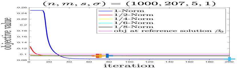
(a) Objective value against the number of iterations

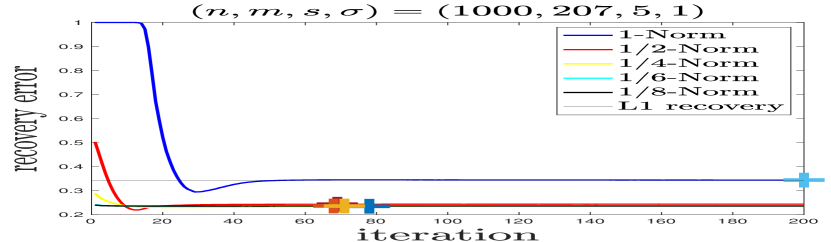
(b) Recovery error against the number of iterations

Figure 1: Performance of pseudo-norm recovery using a power-variable formulation with warm starts. Average over $500$ trials. Each trial’s reference solution $\beta_{0}$ has five nonzero components drawn from the uniform distribution over $[-1,1]$. The last iteration for each value of $\tau$ is averaged over all trials, with the average marked as $+$ in the plot.

5.3 Linear Programming

We consider linear programs (LP) with upper bounds on some variables:

(LP-u) $$\min_{x}\,c^{T}x\;\;\mbox{s.t.}\;\;Ax=b,\;\;0\leq x_{{\cal I}}\leq u,\;\;0\leq x_{{\overline{\cal I}}}.$$

Here ${\cal I}$ is a subset of $[n]$ and ${\overline{\cal I}}$ is its complement. The vector $u\in\mathbb{R}^{|{\cal I}|}$ is the vector of upper bounds. Upper bounds are common in real applications and treating them explicitly can lead to more efficient implementations (see Appendix A). Many of the Netlib problems discussed in Section 5.3.2 are solved more efficiently when upper bounds are allowed in the formulation.

By introducing variables $w$ for the upper bound constraints, we consider a form equivalent to (LP-u):

(LP-uw) $$\min_{x,w}\,c^{T}x\;\;\mbox{s.t.}\;\;Ax=b,\;\;x_{{\cal I}}+w=u,\;\;(x,w)\geq 0,$$

which is in standard form for an linear program (linear equality constraints, with all variables nonnegative). In the SSV form of (LP-uw), the nonnegativity requirements on $x$ and $w$ are replaced by equality constraints $x=v\odot v$ and $w=y\odot y$. We apply the MPC and SSV-SQP approaches introduced in Section 4. Our solvers exploit the structure of the linear constraints in (LP-uw) that arise from the presence of upper bounds. Details are given in Appendix A.

Residuals and stopping criterion

To define the primal-dual residuals, we denote the dual variables for the constraints $x\geq 0$ and $w\geq 0$ as $s\in^{n}$ and $t\in^{|{\cal I}|}$ respectively, and $\lambda$ is the dual variable for the linear constraint $Ax=b$. Define the following residuals:

(66a) $$r_{c_{\cal I}} :=-\mathopen{}\mathclose{{}\left(c_{\cal I}-s_{\cal I}+t-A_{\cal I}\lambda}\right), r_{c_{\overline{\cal I}}} :=-\mathopen{}\mathclose{{}\left(c_{\overline{\cal I}}-s_{\overline{\cal I}}-A_{\overline{\cal I}}\lambda}\right)$$

(66b) $$r_{x} :=-\mathopen{}\mathclose{{}\left(b-Ax}\right), r_{u} :=-\mathopen{}\mathclose{{}\left(u-x_{\cal I}-w}\right),$$

(66c) $$r_{xs} :=x\odot s, r_{rw} :=t\odot w.$$

The residual used to define the stopping criteria is defined as

(67) $$\text{res}:\,=\frac{\lVert(r_{c_{\cal I}},r_{c_{\overline{\cal I}}},r_{x},r_{u},r_{xs},r_{rw},x_{-},w_{-})\rVert}{1+\max\{\lVert b\rVert,\lVert c\rVert\}}.$$

Here $x_{-},w_{-}$ are the negative parts of $x$ and $w$, respectively. Note that we did not consider the nonnegativity of the dual variables $s$ and $t$ because both MPC and SSV-SQP maintain nonnegativity of these variables. We terminate the algorithm when $\text{res}\leq\epsilon$ for some threshold $\epsilon>0$, or when it reaches $2000$ iterations, or $1000$ seconds of CPU-time, whichever comes first.

Parameter choice and initialization

For the step scaling parameter $\tau$, we choose $\tau=\{0.15,0.5,0.75,0.9\}$ for SSV-SQP and $\tau=\{0.9,0.95,0.995\}$ for MPC. For MPC, to initialize $(x,w,\lambda,s,t)$, we define $M:=\max\{\mathopen{}\mathclose{{}\left\|A}\right\|_{\infty},\mathopen{}\mathclose{{}\left\|b}\right\|_{\infty},\mathopen{}\mathclose{{}\left\|c}\right\|_{\infty}\}$ and set $x_{0}=s_{0}=100M\textbf{1}_{n}$ (where $\textbf{1}_{n}$ is the vector of length $n$ whose elements are all $1$), $w_{0}=t_{0}=100M\textbf{1}_{|{\cal I}|}$, and $\lambda=0$. For SSV-SQP, we initialize $(x,w,\lambda,s,t)$ in the same way as MPC. The initial value of the squared variable is taken to be the square root of the corresponding original variable, calculated entrywise.

In the following sections, we report only the number of iterations for MPC and SSV-SQP, not the runtime. The actual runtime for the algorithms to reach a certain accuracy is usually more favorable to SSV-SQP, since it only needs to solve one linear system per iteration, while our naive implementation of MPC factors the coefficient matrix twice at each iteration. Our codes for MPC and SSV-SQP are identical to the extent possible.

5.3.1 Random Linear Programs

We compare the performance of MPC and SSV-SQP on random instances of (LP-u). We choose $n\in\{500,1000,2500\}$, while $m=0.1n$, $0.25n$, and $0.5n$. The number of upper bounds $|{\cal I}|$ is set to be $\lfloor 0.05m\rfloor$. We generate the upper-bounded component indices ${\cal I}$ by randomly drawing from the set $\{1,2,\dotsc,n\}$ without replacement, and choose the upper bounds on these components randomly from a uniform distribution on $[1,21]$. For each combination of $(m,n)$, we randomly generate ten trials of $(A,b,c,{\cal I},u)$. The matrix $A$, vector $c$, and primal feasible point $\tilde{x}$ have entries drawn randomly and i.i.d. from a uniform distribution over $[0,1]$. We set $b:=A\tilde{x}$.

For each choice of parameters and dimensions, we report the average number of iterations over 10 trials to reach a residual smaller than $10^{-8}$ (together with the standard deviation over the 10 trials) for SSV-SQP with $\tau=.5,.75,.9$ and MPC with $\tau=.995$.

The result for random LPs is shown in Table 2. The symbol $*$ indicates that the method fails to reach the desired accuracy in at least one of the ten trials.

$(n,m)$	MPC	SSV ($\tau=.5$)	SSV ($\tau=.75$)	SSV ($\tau=.9$)
(500,50)	15.5 (0.71)	61.0 (2.5)	38.5 (1.8)	$*$
(500,125)	15.8 (0.42)	60.9 (2.4)	39.2 (1.8)	$*$
(500,250)	15.9 (0.32)	61.3 (3.4)	39.4 (2.2)	32.0 (2.2)
(1000,100)	17.1 (0.74)	62.6 (2.2)	39.8 (1.5)	32.5 (1.4)
(1000,250)	17.4 (0.70)	64.8 (3.1)	42.3 (2.9)	35.1 (2.8)
(1000,500)	17.7 (0.48)	64.3 (1.6)	42.4 (1.0)	36.1 (1.4)
(2500,250)	18.2 (0.63)	67.4 (3.4)	43.7 (2.3)	37.0 (2.6)
(2500,625)	18.7 (0.68)	70.1 (2.8)	46.3 (2.2)	38.1 (1.4)
(2500,1250)	18.7 (0.48)	68.3 (2.2)	45.4 (2.1)	39.4 (2.8)

Table 2: Performance of MPC and SSV-SQP for three different values of the parameter $\tau$. Each entry shows average number of iterations together with the standard deviation over ten trials. Missing entries correspond to cases in which convergence was not attained in one or more of the trials.

We note from this table that SSV is consistently slower than MPC, by a factor of 2-4 in the number of iterations. However, this factor was surprisingly modest to us, given the relatively high sophistication and widespread use of the MPC approach (despite our rather elementary implementation), and the lack of tuning of the SSV method. For SSV, the less aggressive value $\tau=.5$ was more reliable in finding a solution, whereas the more aggressive value $\tau=.9$ required approximately half as many iterations, but was less reliable, with the iterates diverging for some trials. (Similar phenomena were noted for non-random problems, as we report below.) The standard deviation of iteration count across trials was slightly higher for SSV than for MPC.

It is possible that the SSV approach could be made significantly more efficient with more sophisticated techniques in SSV-SQP, including an adaptive, varying scheme for choosing the step scaling parameter $\tau$, and other modifications to the basic SQP approach.

5.3.2 Netlib Test Set

We test the performance of SSV-SQP against MPC on the celebrated Netlib test set [4]. which played an important role in the development of interior-point codes for linear programs in the period 1988-1998.

Since the problem data of Netlib usually have some redundancies and degeneracies, which hurts code performance and makes comparisons unreliable, we use the presolver from PCx [2] on each problem. Presolvers typically reduce the problem sizes, eliminate redundancies of many types, and improve the conditioning. This presolver output problems of the upper-bound form (LP-u).

We report the number of instances solved to several accuracies $\epsilon$ for SSV-SQP and MPC in Table 3.. We also report the average number of iterations for the solved instances in Table 4. A report on performances of SSV-SQP and MPC for each instance in Netlib with two of these accuracy levels — $10^{-2}$ and $10^{-5}$ — can be found in Appendix B.

$\epsilon$	$10^{-1}$	$10^{-2}$	$10^{-3}$	$10^{-4}$	$10^{-5}$	$10^{-6}$	$10^{-7}$	$10^{-8}$
$\tau=0.15$	88	88	87	85	83	73	50	22
$\tau=0.5$	88	86	85	83	71	49	26	12
$\tau=0.75$	88	86	81	71	54	28	14	10
$\tau=0.9$	86	82	72	51	31	18	8	2
MPC	88	86	82	81	78	75	72	68

Table 3: The number of cases solved to accuracy $\epsilon$ among $94$ instances for Netlib problems: SSV-SQP with $\tau=0.15$, $0.5$, $0.75$, $0.9$; and MPC with $\tau=0.9$ (last row).

$\epsilon$	$10^{-1}$	$10^{-2}$	$10^{-3}$	$10^{-4}$	$10^{-5}$	$10^{-6}$	$10^{-7}$	$10^{-8}$
$\tau=0.15$	177.2	212.2	242.0	274.2	288.3	315.8	328.4	332.3
$\tau=0.5$	58.3	67.3	79.5	88.5	96.7	94.4	86.8	109.6
$\tau=0.75$	41.5	52.8	59.6	72.4	73.4	53.1	55.4	58.1
$\tau=0.9$	42.8	55.1	60.2	56.4	47.3	45.8	38.6	27.0
MPC	18.8	21.3	23.2	25.3	27.3	28.5	30.1	30.8

Table 4: The average number of iterations among the solved instance with accuracy $\epsilon$ for Netlib problems: SSV-SQP with $\tau=0.15$, $0.5$, $0.75$, $0.9$; and MPC with $\tau=0.9$.

Table 3 shows that as the step-scaling parameter $\tau$ decreases, SSV-SQP is able to solve more problems but requires more iterations. SQP-SSV with $\tau=.15,.5,.75$ is even able to solve more problems than MPC for less stringent tolerances $(10^{-1}$-$10^{-2})$. SQP-SSV with $\tau=.5$ is also able to solve at least as many instances as MPC for accuracies $10^{-1}$-$10^{-4}$. Table 4 shows that for $\tau=0.5$, the number of iterations of SSV-SQP is within a factor of $4$ of that for MPC. For $\tau=0.9$, among solved instances, SSV-SQP is even more competitive with MPC, but for smaller values of $\epsilon$, many problem instances are not solved by SSV-SQP. The number of iterations required by SSV-SQP for the most conservative setting $\tau=.15$ is much worse, averaging a factor of about 10 greater than MPC.

Details of the experience with Netlib problems for two values of $\epsilon$, $10^{-2}$ and $10^{-5}$, are shown in Table LABEL:tb:_netlib_MPCvsSSV in Appendix B.

We note the low success rates for SSV-SQP with higher accuracies (smaller $\epsilon$). We believe that with tuning we could certainly improve the performance of both codes, especially SSV-SQP, for which (by contrast with MPC) there is no “folklore” concerning heuristics that improve efficiency.

6 Conclusions

We have considered both theoretical and practical aspects of squared-variables formulations for inequality-constrained optimization problems. Building on previous work, we find that some of the theoretical drawbacks are less problematic than conventional wisdom would suggest. Practically, although squared-variable approaches do not improve on the state of the art in quadratic and linear programming, they are more competitive than might be expected, and may with further development prove to be useful in some circumstances. In the case of pseudo-norm constrained least squares (a problem of interest in sparse recovery) an extension of the squared-variable approach has good computational performance.

Appendix A PDIP, MPC, and SSV for LP with upper bounds

We derive the formulas of one iteration for PDIP, MPC, and SSV-SQP for (LP-uw).

A.1 PDIP

We introduce dual variables $\lambda\in\mathbb{R}^{m}$ for $Ax=b$, $s\in\mathbb{R}^{n}$ for $x\geq 0$, $t\in\mathbb{R}^{|{\cal I}|}$ for $w\geq 0$. The KKT condition for (LP-uw) is

(68a) $$A^{T}_{{\cal I}}\lambda+s_{\cal I}-t-c_{\cal I} =0,$$

(68b) $$A^{T}_{{\overline{\cal I}}}\lambda+s_{\overline{\cal I}}-c_{\overline{\cal I}} =0,$$

(68c) $$Ax-b =0,$$

(68d) $$x_{{\cal I}}+w =u,$$

(68e) $$s\odot x =0,\quad w\odot t=0$$

(68f) $$(x,s,t,w) \geq 0.$$

Here $A_{{\cal I}}$ and $A_{{\overline{\cal I}}}$ are columns of $A$ in $I$ and $J$ respectively.

Each iteration of PDIP for (68) aims to solve:

(69a) $$A^{T}_{{\cal I}}\Delta\lambda+\Delta s_{\cal I}-\Delta r =-r_{c_{\cal I}}:\,=c_{\cal I}-s_{\cal I}+t-A_{\cal I}\lambda,$$

(69b) $$A^{T}_{{\overline{\cal I}}}\Delta\lambda+\Delta s_{\overline{\cal I}} =-r_{c_{\overline{\cal I}}}:\,=c_{\overline{\cal I}}-s_{\overline{\cal I}}-A_{\overline{\cal I}}\lambda$$

(69c) $$A\Delta x =-r_{x}:\,=b-Ax,$$

(69d) $$\Delta x_{{\cal I}}+\Delta w =-r_{u}:\;=u-x_{\cal I}-w,$$

(69e) $$X\Delta s+S\Delta x =-r_{xs}:\;=-x\odot s+\sigma(s^{T}x+w^{T}t)/(n+|{\cal I}|),$$

(69f) $$W\Delta r+T\Delta W =-r_{rw}:\;=-t\odot w+\sigma(s^{T}x+w^{T}t)/(n+|{\cal I}|),$$

where $X=\operatorname{diag}(x)$, $S=\operatorname{diag}(s)$, $W=\operatorname{diag}(w)$ and $T=\operatorname{diag}(t)$, and $\sigma\in[0,1]$ is some centering parameter. All components of $x$, $s$, $t$, and $w$ are maintained strictly positive throughout.

Let $r_{xwr}\in\mathbb{R}^{n}$ such that

(70) $$r_{xwr,{\cal I}}=X_{{\cal I}}^{-1}r_{xs,{\cal I}}-W^{-1}r_{rw}+W^{-1}Tr_{u}-r_{c_{\cal I}},$$

and

(71) $$r_{xwr,{\overline{\cal I}}}=X_{{\overline{\cal I}}}^{-1}r_{xs,{\overline{\cal I}}}-r_{c_{\cal I}}.$$

Here $X_{{\cal I}}=\operatorname{diag}(x_{{\cal I}})$ and $X_{{\overline{\cal I}}}=\operatorname{diag}(x_{{\cal I}}).$ Let $D\in\mathbb{R}^{n\times n}$ be a diagonal matrix such that

(72) $$D_{{\cal I},{\cal I}}=X_{{\cal I}}^{-1}S_{{\cal I}}+W^{-1}T,\quad\text{and}\quad D_{{\overline{\cal I}},{\overline{\cal I}}}=X_{{\overline{\cal I}}}^{-1}S_{{\overline{\cal I}}}.$$

Here $D_{{\cal I},{\cal I}}$ is the block corresponding to the index set ${\cal I}$ and $D_{{\overline{\cal I}},{\overline{\cal I}}}$ is the block corresponding to the index set ${\overline{\cal I}}$.

After a series of eliminationn in (69), we obtain $\Delta x$ and $\Delta\lambda$ by solving

(73) $$\begin{bmatrix}-D&A^{\top}\\ A&0\end{bmatrix}\begin{bmatrix}\Delta x\\ \Delta\lambda\end{bmatrix}=\begin{bmatrix}r_{vwr}\\ -r_{x}\end{bmatrix}.$$

One can then easily solve for $\Delta w$, $\Delta t$, and $\Delta s$. Reducing further, we obtain the system

(74) $$AD^{-1}A^{\top}\Delta\lambda=AD^{-1}r_{vwr}-r_{x},$$

which is the form often considered in production interior-point software. We use (73) in the experiments for the Netlib data set because this system yields more accurate solutions in a finite-precision setting than (74) [16, 17]. We take steps of the form $(x,w)+\alpha_{P}(\Delta x,\Delta w)$ and $(\lambda,s,t)+\alpha_{D}(\Delta\lambda,\Delta s,\Delta t)$. We choose $\alpha_{P}$ and $\alpha_{D}$ similarly to (56) and (57). Precisely, we set the maximum step for primal and dual as

$$\mbox{PDIP:}\quad\alpha_{P}^{\max} =\min\mathopen{}\mathclose{{}\left(1,\max\{\alpha\mid(x,w)+\alpha(\Delta x,\Delta w)\geq 0\}}\right),$$

$$\mbox{PDIP:}\quad\alpha_{D}^{\max} =\min\mathopen{}\mathclose{{}\left(1,\max\{\alpha\mid(s,t)+\alpha(\Delta s,\Delta t)\geq 0\}}\right),$$

then choose the actual steplengths to be

$$\mbox{PDIP:}\quad\alpha_{P}=\tau\alpha_{P}^{\max},\quad\text{and}\quad\alpha_{D}=\tau\alpha_{D}^{\max},$$

for some parameter $\tau\in[0,1)$.

A.2 MPC

The MPC updates the iterates $(x,w,\lambda,s,t)$ by solving the system (69) twice with a different right-hand side each time. We spell out the details here by following [15, Chapter 10]. First, MPC obtained an affine-scaling direction $(\Delta x^{\text{aff}},\Delta w^{\text{aff}},\Delta\lambda^{\text{aff}},\Delta s^{\text{aff}},\Delta t^{\text{aff}})$ by solving (69) with $\sigma=0$. Next, it computes primal and dual stepsize for these two directions:

$$\alpha_{P}^{\text{aff}} =\min\mathopen{}\mathclose{{}\left(1,\max\{\alpha\mid x+\alpha\Delta x^{\text{aff}}\geq 0,w+\alpha\Delta w^{\text{aff}}\geq 0\}}\right),$$

$$\quad\alpha_{D}^{\text{aff}} =\min\mathopen{}\mathclose{{}\left(1,\max\{\alpha\mid s+\alpha\Delta s^{\text{aff}}\geq 0,t+\alpha\Delta t^{\text{aff}}\geq 0\}}\right).$$

After computing the affine-scaling stepsizes, it computes a duality gap for the affine-scaling updates:

$$\mu_{\text{aff}}=\frac{(x+\alpha_{P}^{\text{aff}}\Delta x^{\text{aff}})^{\top}(s+\alpha_{D}^{\text{aff}}\Delta s^{\text{aff}})+(w+\alpha_{P}^{\text{aff}}\Delta w^{\text{aff}})^{\top}(t+\alpha_{D}^{\text{aff}}\Delta t^{\text{aff}})}{n+|{\cal I}|}.$$

Then it obtains the actual search direction $(\Delta x,\Delta w,\Delta\lambda,\Delta s,\Delta t)$ by solving the system (69) again with $\sigma$ set as follows:

(75) $$\sigma=\mathopen{}\mathclose{{}\left(\frac{\mu_{\text{aff}}}{\mu}}\right)^{3},\quad\text{where}\quad\mu=\frac{x^{\top}s+w^{\top}t}{n+|{\cal I}|}.$$

It then sets the maximum stepsize for primal and dual as

$$\mbox{MPC:}\quad\alpha_{P}^{\max} =\min\mathopen{}\mathclose{{}\left(1,\max\{\alpha\mid(x,w)+\alpha(\Delta x,\Delta w)\geq 0\}}\right),$$

$$\mbox{MPC:}\quad\alpha_{D}^{\max} =\min\mathopen{}\mathclose{{}\left(1,\max\{\alpha\mid(s,t)+\alpha(\Delta s,\Delta t)\geq 0\}}\right),$$

and takes the actual step length to be

$$\mbox{MPC:}\quad\alpha_{P}=\tau\alpha_{P}^{\max},\quad\text{and}\quad\alpha_{D}=\tau\alpha_{D}^{\max},$$

for some parameter $\tau\in[0,1)$. We then update the primal and dual variables as follows: $(x,w)+\alpha_{P}(\Delta x,\Delta w)$ and $(\lambda,s,t)+\alpha_{D}(\Delta\lambda,\Delta s,\Delta t)$.

A.3 SSV-SQP

We first introduce the squared variables for (LP-uw) and obtain

(LP-uw-ssv) $$\text{minimize}_{x\in\mathbb{R}^{n}} \quad c^{T}x$$

subject to $$\quad Ax=b,$$

$$\quad u=w+x_{{\cal I}}$$

$$\quad x=v\odot v\quad\text{and}\quad w=y\odot y.$$

KKT conditions for (LP-uw-ssv) is

(76a) $$A^{T}_{{\cal I}}\lambda+s_{\cal I}-t-c_{\cal I} =0,$$

(76b) $$A^{T}_{{\overline{\cal I}}}\lambda+s_{\overline{\cal I}}-c_{\overline{\cal I}} =0,$$

(76c) $$Ax-b =0,$$

(76d) $$x_{{\cal I}}+w =u,$$

(76e) $$s\odot v=0,\quad y\odot r=0$$

(76f) $$x=v\odot v,\quad w=y\odot y.$$

Each iteration of SQP for (76) aims to solve:

(77a) $$A^{T}_{{\cal I}}\Delta\lambda+\Delta s_{\cal I}-\Delta t =-r_{c_{\cal I}}:\,=c_{\cal I}-s_{\cal I}+t-A_{\cal I}\lambda,$$

(77b) $$A^{T}_{{\overline{\cal I}}}\Delta\lambda+\Delta s_{\overline{\cal I}} =-r_{c_{\overline{\cal I}}}:\,=c_{\overline{\cal I}}-s_{\overline{\cal I}}-A_{\overline{\cal I}}\lambda$$

(77c) $$A\Delta x =-r_{x}:\,=b-Ax,$$

(77d) $$\Delta x_{{\cal I}}+\Delta w =-r_{u}:\;=u-x_{\cal I}-w,$$

(77e) $$V\Delta s+S\Delta x =-r_{sv}:\;=-v\odot s,$$

(77f) $$Y\Delta t+T\Delta W =-r_{ry}:\;=-t\odot y,$$

(77g) $$\Delta x-2v\odot\Delta v =-r_{v}:\;=-x+v\odot v,$$

(77h) $$\Delta w+2y\odot\Delta y =-r_{y}:\;=-w+y\odot y.$$

where $V=\operatorname{diag}(v)$, $S=\operatorname{diag}(s)$, $Y=\operatorname{diag}(y)$, and $T=\operatorname{diag}(t)$. We maintain strict positivity of all components of $v$, $s$, $y$, and $t$ at all iterations.

Let $r_{vwr}\in\mathbb{R}^{n}$ such that

(78) $$r_{vwr,{\cal I}}=V_{{\cal I}}^{-1}r_{sv,{\cal I}}-Y^{-1}r_{ry}+\tfrac{1}{2}V_{{\cal I}}^{-2}S_{{\cal I}}r_{v,{\cal I}}-\tfrac{1}{2}Y^{-2}Tr_{y}+\tfrac{1}{2}Y^{-2}Tr_{u}-r_{c_{\cal I}},$$

and

(79) $$r_{vwr,{\overline{\cal I}}}=V_{{\overline{\cal I}}}^{-1}r_{sv,{\overline{\cal I}}}+\tfrac{1}{2}V_{{\overline{\cal I}}}^{-2}S_{{\overline{\cal I}}}r_{v,{\overline{\cal I}}}-r_{c_{\overline{\cal I}}}.$$

Here $V_{{\cal I}}=\operatorname{diag}(v_{{\cal I}})$, $V_{{\overline{\cal I}}}=\operatorname{diag}(v_{{\cal I}})$, $S_{{\cal I}}=\operatorname{diag}(s_{{\cal I}})$, and $S_{{\overline{\cal I}}}=\operatorname{diag}(s_{{\overline{\cal I}}})$. Let $D\in\mathbb{R}^{n\times n}$ be the diagonal matrix whose diagonal blocks are

(80) $$D_{{\cal I},{\cal I}}=\tfrac{1}{2}V_{{\cal I}}^{-2}S_{{\cal I}}+\tfrac{1}{2}Y^{-2}T,\quad\text{and}\quad D_{{\overline{\cal I}},{\overline{\cal I}}}=\tfrac{1}{2}V_{{\overline{\cal I}}}^{-2}S_{{\overline{\cal I}}}.$$

Here $D_{{\cal I},{\cal I}}$ is the block corresponding to the index set ${\cal I}$ and $D_{{\overline{\cal I}},{\overline{\cal I}}}$ is the block corresponding to the index set ${\overline{\cal I}}$.

After a series of elimination for (77), we obtain $\Delta x$ and $\Delta\lambda$ by solving

(81) $$\begin{bmatrix}-D&A^{\top}\\ A&0\end{bmatrix}\begin{bmatrix}\Delta x\\ \Delta\lambda\end{bmatrix}=\begin{bmatrix}r_{vwr}\\ -r_{x}\end{bmatrix}.$$

One can recover the other step components. Reducing further, we obtain the system

(82) $$AD^{-1}A^{\top}\Delta\lambda=AD^{-1}r_{xwr}-r_{x}.$$

We use (81) in the experiments for the Netlib data set because this system yields more accurate solutions in a finite-precision setting than (82). We update primal and dual variables via $(x,w,y,v)+\alpha_{P}(\Delta x,\Delta w,\Delta y,\Delta v)$ and $(\lambda,s,t)+\alpha_{D}(\Delta\lambda,\Delta s,\Delta t)$. The actual stepsizes $\alpha_{P}$ and $\alpha_{D}$ are chosen similarly to (58) and (59). We set the maximum step for primal and dual as

$$\mbox{SSV-SQP:}\quad\alpha_{P}^{\max} =\min\mathopen{}\mathclose{{}\left(1,\max\{\alpha\mid(v,y)+\alpha(\Delta v,\Delta y)\geq 0\}}\right),$$

$$\mbox{SSV-SQP:}\quad\alpha_{D}^{\max} =\min\mathopen{}\mathclose{{}\left(1,\max\{\alpha\mid(s,t)+\alpha(\Delta s,\Delta t)\geq 0\}}\right),$$

with actual step lengths defined as

$$\mbox{SSV-SQP:}\quad\alpha_{P}=\tau\alpha_{P}^{\max},\quad\text{and}\quad\alpha_{D}=\tau\alpha_{D}^{\max},$$

where $\tau\in(0,1]$ is a fixed parameter.

Appendix B Results of SSV-SQP and MPC for each problem in Netlib

Table LABEL:tb:_netlib_MPCvsSSV shows the number of iterations for each problem in Netlib of SSV-SQP with $\tau=0.5,\;0.75.\;0.9$ and MPC with $\tau=0.9$ for accuracy parameters $10^{-2}$ and $10^{-5}$. The problem dimensions $(m,n)$ are for the presolved versions, obtained from the presolver of PCx [2].

Table 5: The number of iterations of SSV-SQP (with $\tau=.5,.75,.9$) and MPC (with $\tau=.9$) for different problems in Netlib in terms of accuracy levels $\epsilon=10^{-2}$ and $\epsilon=10^{-5}$. For each value of $\epsilon$, we display the number of iterations for SSV-SQP (with $\tau=.5,.75,.9$) and MPC (with $\tau=.9$) from left to right. $*$ indicates the algorithm cannot attain the desired accuracy within $2000$ iterations or $1000$ seconds in terms of CPU time. For example, for $\epsilon=10^{-2}$ and the instance 25fv47, we have the number of iterations for SSV-SQP with $\tau=.5,.75,.9$ being 65, 66, and 57, and the number of iterations for MPC with $\tau=.9$ is 25. Problem names displayed with a superscript ”$+$” are those for which SSV-SQP solves the problem successfully for $\epsilon=10^{-5}$ when $\tau=.15$, though unsuccessful for larger values of $\tau$.

Name	$(n,m)$	$\epsilon=10^{-2}$				$\epsilon=10^{-5}$
25fv47	(1843,788)	65	66	57	25	120	$*$	$*$	34
80bau3b+	(11066,2140)	206	136	131	$*$	$*$	$*$	$*$	$*$
adlittle	(137,55)	44	29	24	18	54	35	$*$	22
afiro	(51,27)	34	21	17	14	47	29	23	17
agg2	(750,514)	93	63	52	27	109	76	67	33
agg3	(750,514)	86	60	52	26	102	71	68	32
agg	(477,390)	68	48	43	25	80	56	51	31
bandm	(395,240)	69	51	48	18	83	61	$*$	24
beaconfd	(171,86)	54	33	27	16	64	38	31	21
blend	(111,71)	40	26	24	14	55	36	$*$	18
bnl1+	(1491,610)	54	39	35	28	$*$	$*$	$*$	40
bnl2	(4008,1964)	103	125	154	30	214	185	$*$	44
boeing1	(697,331)	49	37	35	19	99	69	$*$	27
boeing2	(264,125)	60	49	49	20	$*$	$*$	$*$	27
bore3d	(138,81)	49	33	29	21	63	41	33	24
brandy	(238,133)	56	39	37	19	82	59	$*$	$*$
capri	(436,241)	100	84	92	23	117	97	$*$	29
cycle	(2780,1420)	$*$	129	$*$	33	$*$	$*$	$*$	$*$
czprob	(2779,671)	51	37	34	33	65	46	41	40
d2q06c	(5728,2132)	83	66	96	30	132	$*$	$*$	$*$
d6cube	(5443,403)	37	24	20	16	72	53	53	32
degen2	(757,444)	28	18	14	14	51	34	30	21
degen3	(2604,1503)	32	21	18	17	63	$*$	41	25
dfl001	(12143,5984)	$*$	$*$	$*$	$*$	$*$	$*$	$*$	$*$
e226	(429,198)	41	26	22	17	67	48	43	24
etamacro+	(669,334)	46	31	27	19	$*$	$*$	$*$	29
fffff800	(826,322)	87	66	61	33	114	$*$	$*$	39
finnis+	(935,438)	84	67	69	26	$*$	$*$	$*$	31
fit1d	(1049,24)	36	22	19	19	50	32	27	26
fit1p	(1677,627)	94	85	$*$	19	104	95	$*$	24
fit2d	(10524,25)	40	25	24	20	56	40	43	28
fit2p	(13525,3000)	67	72	96	20	86	$*$	$*$	26
forplan	(447,121)	53	33	31	22	82	57	53	$*$
ganges	(1510,1113)	52	35	32	18	96	68	63	23
gfrd-pnc	(1134,590)	76	60	59	22	157	123	122	26
greenbea	(4164,1933)	101	$*$	$*$	40	$*$	$*$	$*$	47
greenbeb+	(4155,1932)	107	83	83	42	$*$	$*$	$*$	$*$
grow15	(645,300)	$*$	$*$	$*$	33	$*$	$*$	$*$	38
grow22	(946,440)	$*$	$*$	$*$	34	$*$	$*$	$*$	39
grow7	(301,140)	$*$	$*$	$*$	32	$*$	$*$	$*$	36
israel	(316,174)	85	66	64	25	107	$*$	$*$	29
kb2	(68,43)	37	26	23	15	51	32	26	19
lotfi	(346,133)	69	50	48	17	87	63	$*$	25
maros-r7	(7440,2152)	98	110	132	18	127	134	153	25
maros	(1437,655)	56	35	28	$*$	105	$*$	$*$	$*$
modszk1	(1599,665)	168	133	109	22	280	267	$*$	29
nesm+	(2922,654)	51	33	37	24	$*$	$*$	$*$	34
perold	(1462,593)	118	83	73	$*$	154	$*$	$*$	$*$
pilot-ja+	(1892,810)	88	65	63	$*$	$*$	$*$	$*$	$*$
pilot-we	(2894,701)	124	94	143	$*$	145	121	$*$	$*$
pilot4	(1110,396)	132	96	88	24	183	134	$*$	34
pilot87	(6373,1971)	140	112	93	27	275	267	$*$	35
pilot	(4543,1368)	95	67	59	30	215	170	$*$	46
recipelp	(123,64)	34	16	12	11	45	27	21	15
sc105	(162,104)	33	19	14	13	57	35	27	18
sc205	(315,203)	42	28	23	14	80	54	42	20
sc50a	(77,49)	35	24	19	13	49	31	25	17
sc50b	(76,48)	32	21	17	13	44	26	20	17
scagr25	(669,469)	52	35	30	19	64	43	36	24
scagr7	(183,127)	47	36	31	18	64	44	36	22
scfxm1	(568,305)	67	52	55	22	86	65	$*$	28
scfxm2	(1136,610)	81	64	58	23	105	89	$*$	31
scfxm3	(1704,915)	80	62	59	23	108	94	96	31
scorpion	(412,340)	$*$	$*$	$*$	$*$	$*$	$*$	$*$	$*$
scrs8	(1199,421)	141	123	$*$	22	198	$*$	$*$	30
scsd1	(760,77)	30	20	16	10	45	$*$	$*$	15
scsd6	(1350,147)	31	21	18	10	46	30	$*$	17
scsd8+	(2750,397)	32	22	18	12	$*$	$*$	$*$	16
sctap1+	(644,284)	56	40	39	18	$*$	$*$	$*$	24
sctap2	(2443,1033)	50	38	41	17	128	$*$	$*$	22
sctap3+	(3268,1408)	52	40	42	18	$*$	$*$	$*$	23
seba	(901,448)	53	37	33	20	68	45	39	23
share1b	(248,112)	55	40	38	22	76	53	$*$	28
share2b+	(162,96)	33	22	18	15	$*$	$*$	$*$	19
shell	(1451,487)	93	78	79	31	106	$*$	$*$	35
ship04l	(1905,292)	84	94	177	18	94	99	$*$	22
ship04s	(1281,216)	70	68	167	18	81	74	$*$	22
ship08l	(3121,470)	105	120	230	19	122	129	$*$	$*$
ship08s	(1604,276)	65	55	125	18	77	60	$*$	$*$
ship12l	(4171,610)	107	103	183	19	120	$*$	$*$	24
ship12s	(1943,340)	65	59	74	18	79	67	$*$	23
sierra	(2705,1212)	$*$	$*$	$*$	$*$	$*$	$*$	$*$	$*$
stair	(538,356)	44	26	19	16	79	49	40	23
standata	(796,314)	61	46	52	23	80	$*$	$*$	27
standgub	(796,314)	61	46	52	23	80	$*$	$*$	27
standmps+	(1192,422)	66	49	$*$	29	$*$	$*$	$*$	42
stocfor1	(150,102)	40	26	22	18	55	$*$	$*$	22
stocfor2	(2868,1980)	71	60	62	22	112	$*$	$*$	29
stocfor3	(22228,15362)	$*$	$*$	$*$	27	$*$	$*$	$*$	$*$
truss+	(8806,1000)	45	34	31	16	$*$	$*$	$*$	23
tuff	(567,257)	45	30	26	18	111	78	$*$	28
vtp-base	(111,72)	44	30	25	17	54	35	28	20
wood1p	(1718,171)	51	31	25	24	76	49	43	41
woodw	(5364,708)	27	17	14	18	66	48	45	31

References

• [1] D. P. Bertsekas, Nonlinear Programming, Athena Scientific, second ed., 1999.
• [2] J. Czyzyk, S. Mehrotra, M. Wagner, and S. J. Wright, Pcx: An interior-point code for linear programming, Optimization Methods and Software, 11 (1999), pp. 397–430.
• [3] E. H. Fukuda and M. Fukushima, A note on the squared slack variables technique for nonlinear optimization, Journal of the Operations Research Society of Japan, 60 (2017), pp. 262–270.
• [4] D. M. Gay, Electronic mail distribution of linear programming test problems, Mathematical Programming Society COAL Newsletter, 13 (1985), pp. 10–12.
• [5] P. E. Gill, W. Murray, and M. H. Wright, Practical Optimization, Academic Press, 1981.
• [6] T. M. Inc., Matlab version: 9.10 (r2022a), 2021, https://www.mathworks.com.
• [7] E. Levin, J. Kileel, and N. Boumal, The effect of smooth parametrizations on nonconvex optimization landscapes, arXiv preprint arXiv:2207.03512, (2022).
• [8] Q. Li, D. McKenzie, and W. Yin, From the simplex to the sphere: Faster constrained optimization using the Hadamard parametrization, arXiv preprint arXiv:2112.05273, (2021).
• [9] S. Mehrotra, On the implementation of a primal-dual interior point method, SIAM Journal on optimization, 2 (1992), pp. 575–601.
• [10] C. W. Royer, M. O’ Neill, and S. J. Wright, A Newton-CG algorithm with complexity guarantees for smooth unconstrained optimization, Mathematical Programming, 180 (2020), pp. 451–488.
• [11] R. A. Tapia, A stable approach to Newton’s method for general mathematical programming problems in $\mathbb{R}^{n}$, Journal of Optimization Theory and Applications, 14 (1974), pp. 453–476.
• [12] R. A. Tapia, On the role of slack variables in quasi-Newton methods for constrained optimization, in Numerical Optimisation of Dynamic Systems, L. C. W. DIxon and G. P. Szegö, eds., North-Holland, 1980, pp. 235–246.
• [13] R. Tibshirani, Regression shrinkage and selection via the Lasso, Journal of the Royal Statistical Society: Series B (Methodological), 58 (1996), pp. 267–288.
• [14] A. Wächter and L. T. Biegler, On the implementation of a primal-dual interior point filter line search algorithm for large-scale nonlinear programming, Mathematical Programming, Series B, 106 (2006), pp. 25–57.
• [15] S. J. Wright, Primal-Dual Interior-Point Methods, SIAM, Philadelphia, PA, 1997.
• [16] S. J. Wright, Stability of augmented system factorizations in interior-point methods, SIAM Journal on Matrix Analysis and Applications, 18 (1997), pp. 191–222.
• [17] S. J. Wright, Modified cholesky factorizations in interior-point algorithms for linear programming, SIAM Journal on Optimization, 9 (1999), pp. 1159–1191.
• [18] Y. Xie and S. J. Wright, Complexity of proximal augmented Lagrangian for nonconvex optimization with nonlinear equality constraints, Journal of Scientific Computing, 86 (2021), pp. 1–30.