STAMP: Differentiable Task and Motion Planning via Stein Variational Gradient Descent

Abstract

Planning for many manipulation tasks, such as using tools or assembling parts, often requires both symbolic and geometric reasoning. Task and Motion Planning (TAMP) algorithms typically solve these problems by conducting a tree search over high-level task sequences while checking for kinematic and dynamic feasibility. This can be inefficient as the width of the tree can grow exponentially with the number of possible actions and objects. In this paper, we propose a novel approach to task and motion planning (TAMP) that relaxes discrete-and-continuous TAMP problems into inference problems on a continuous domain. Our method, Stein Task and Motion Planning (STAMP) subsequently solves this new problem using a gradient-based variational inference algorithm called Stein Variational Gradient Descent, by obtaining gradients from a parallelized differentiable physics simulator. By introducing relaxations to the discrete variables, leveraging parallelization, and approaching TAMP as an Bayesian inference problem, our method is able to efficiently find multiple diverse plans in a single optimization run. We demonstrate our method on two TAMP problems and benchmark them against existing TAMP baselines.

I Introduction

TAMP for robotics is a family of algorithms that conduct integrated logical and geometric reasoning, resulting in a symbolic action plan and a motion plan that are feasible and solve a particular goal [1]. Prior works such as [2, 3, 4] ultimately solve TAMP problems by conducting a tree search over discrete logical plans and integrating this with motion optimization and feasibility checking. While these works have shown success in solving a number of difficult problems, including long-horizon planning with tools [4], such an approach to TAMP has several limitations. First, the search over discrete symbolic plans can become highly inefficient, because the width of the tree can grow exponentially with the number of objects and possible successor states. Second, many TAMP algorithms with the exception of stochastic TAMP methods such as [5, 6] are deterministic and produce a single plan, and thus have a limited ability to deal with uncertainty in partially observable settings or settings with stochastic dynamics. On the other hand, while stochastic TAMP methods have the ability to deal with uncertain observations and dynamics, they are often computationally expensive [7].

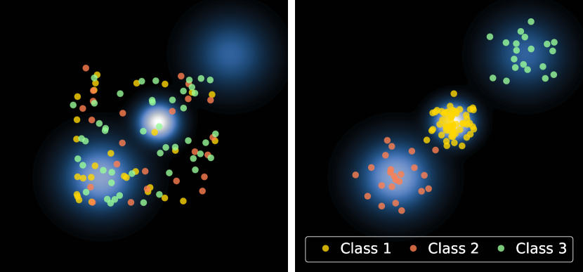
Figure 1: Fitting a Gaussian mixture with discrete-and-continuous SVGD. Left: random initialization of particles. Right: particles after 500 updates. In TAMP, classes 1-3 are analogous to the discrete symbolic plans while the particles’ positions are analogous to the continuous motion plans. The target distribution is analogous to a posterior distribution over the task and motion plan conditioned on the plan being optimal. In other words, higher density regions in the posterior correspond to plans that better solve the problem.

In this paper, we present a novel algorithm for TAMP called Stein Task and Motion Planning (STAMP) that is both efficient and able to produce a distribution of optimal plans. Unlike traditional TAMP algorithms, STAMP solves TAMP in a fully differentiable manner, forgoing the need to conduct a computationally expensive search over discrete task plans integrated with motion planning. Further, it solves TAMP as a Bayesian inference problem that is parallelized on the GPU. These two factors combined allow STAMP to efficiently find a diverse set of plans in one algorithm run.

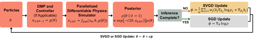
Figure 2: Overview of STAMP algorithm pipeline. The particles $\theta$ denote the action sequences and their parameters.

The main contributions of our work are (a) formulating TAMP as a Bayesian inference problem over continuous variables by relaxing the discrete symbolic actions into the continuous domain; (b) solving the new TAMP problem via a gradient-based inference algorithm, leveraging the end-to-end differentiability of differentiable physics simulators; and (c) parallelizing the inference process so that multiple diverse plans can be found in one optimization run. Our approach builds on top of a variational inference algorithm known as Stein variational gradient descent (SVGD) [8, 9] and uses a parallelized differentiable physics simulator [10]. These two ingredients allow us to approach TAMP as a probabilistic inference problem that can be solved using gradients, in parallel. In addition, we employ imitation learning to introduce action abstractions that reduce the high-dimensional variational inference problem over long trajectories to a low-dimensional inference problem. We compare our algorithm to logic-geometric programming (LGP) [4] and PDDLStream [3], two prominent TAMP baselines, and show that our method outperforms both algorithms in terms of the time required to generate a diversity of feasible plans.

II Related Work

There are many important prior works in the domain of task and motion planning. [1] [1] provide a good overview. A fundamental problem in TAMP is selecting real-valued parameters that define the mode of the motion bridging the motion planning problem with a high-level symbol. One solution introduced in PDDLStream [3] is to sample these parameters, such as an object’s grasp pose and a trajectory’s goal pose. Then, the problem can be reduced to a sequence of PDDL problems [11] and solved with a traditional symbolic planner. Our method is more closely related to a class of TAMP solvers known as LGP [4, 12, 13, 14, 15], which optimize the motion plan directly on the geometric level to minimize an arbitrary cost function. Logical states then define various kinematic, dynamic, and mode transition constraints on the trajectories. There are several extensions to this line of work. [4] [4] incorporate differentiable simulators to LGP for planning tool uses. [15] [15] introduce probabilistic LGP for uncertain environments and [13] [13] extend LGP with force-based reasoning to directly optimize physically plausible trajectories. While LGP uses branch-and-bound and tree search to solve the optimization problem, our method uses gradients from a differentiable simulator to directly optimize motions and (relaxed) symbolic variables.

Many recent works on differentiable simulators [16, 17, 18, 19, 10] have shown that they can be used to optimize trajectories [20], controls [21], or policies [22] directly. [23] [23] also use Stein variational gradient descent [8] with gradients from differential simulators for system identification. Similar to our approach, their reason for using SVGD as the inference tool is its ability to find a globally optimal distribution from local gradients. [24] [24] show that SVGD can also solve short-horizon trajectory optimizations probabilistically for model predictive control. In contrast, we optimize both high-level symbolic and detailed motion plans with differentiable simulators.

Similar to our work, [25] [25] developed a differentiable TAMP method. Their idea is to relax the kinematic switches and thereby transform TAMP into a continuous optimization problem that can be solved with gradients, using algorithms like Newton’s Method. They do not explicitly solve for task assignments and instead allow them to emerge naturally from solving the continuous optimization problem. In contrast to their approach, we introduce relaxations to the symbolic tasks, optimize for the task plan directly, and approach TAMP as a variational inference problem that is solved with a gradient-based inference algorithm. Further, unlike their approach, our algorithm finds for multiple diverse plans in parallel.

III Preliminaries

III-A Stein Variational Gradient Descent

SVGD is a variational inference algorithm that uses samples (also called particles) to fit a target distribution. Running inference via SVGD involves randomly initializing a set of samples and then updating them iteratively, using gradients of the target distribution [8]. SVGD’s iterative updates resemble gradient descent and are derived by minimizing the Kullback-Leibler (KL) divergence between the sample distribution and the target distribution within a function space [8]. SVGD is fast, parallelizable, and can be used to fit both continuous and discrete distributions. In the following, we will introduce these two flavors of SVGD.

III-A1 SVGD for Continuous Distributions [8]

Given a target distribution $p(x)$, $x\in\mathbb{R}^{d}$, a randomly initialized set of samples $\{x_{i}\}_{i=1}^{n}$, a positive definite kernel $k(x,x^{\prime})$, and a learning rate $\epsilon$, SVGD iteratively applies the following update rule on $\{x_{i}\}_{i=1}^{n}$ to approximate the target distribution $p(x)$ (where $k_{ji}=k(x_{j},x_{i})$ for brevity):

$$x_{i}\leftarrow x_{i}+\frac{\epsilon}{n}\sum_{j=1}^{n}\bigl{[}\nabla_{x_{j}}\log p(x_{j})k_{ji}+\nabla_{x_{j}}k_{ji}\bigr{]},$$ (1)

III-A2 SVGD for Discrete Distributions [9]

The aim of SVGD for discrete distributions (DSVGD) is to approximate a target distribution $p_{*}(z)$ on a discrete set $\mathcal{Z}=\{z_{1},\dots,z_{K}\}$. To employ a similar gradient-based update rule to SVGD, DSVGD relies on the construction of a differentiable and continuous distribution $\rho(x)$, $x\in\mathbb{R}^{d}$, that mimics the discrete distribution $p_{*}(z)$. A crucial step in creating the surrogate, $\rho(x)$, from $p_{*}(z)$ is to find a map $\Gamma:\mathbb{R}^{d}\rightarrow\mathcal{Z}$ that divides a base distribution $p_{0}(x)$ (which can be any distribution, e.g., a Gaussian) into $K$ partitions that have equal probability. That is,

$$\int_{\mathbb{R}^{d}}p_{0}(x)\,\mathbb{I}[z_{i}=\Gamma(x)]\,\mathrm{d}x=1/K.$$ (2)

Given this map, the authors of [9] suggest

$$\rho(x)\propto p_{0}(x)\tilde{p}_{*}\big{(}\tilde{\Gamma}(x)\big{)}$$ (3)

as one possibility of creating $\rho(x)$, where $\tilde{p}_{*}(\cdot)$ and $\tilde{\Gamma}(\cdot)$ are smooth and differentiable approximations of ${p}_{*}(\cdot)$ and ${\Gamma}(\cdot)$, respectively. DSVGD uses the surrogate to update the samples via the following (where $k_{ji}=k(x_{j},x_{i})$ and $w=\sum_{i}w_{i}$ for brevity).

$$\begin{gathered}x_{i}\leftarrow x_{i}+\frac{\epsilon}{w}\sum_{j=1}^{n}w_{j}\big{(}\nabla_{x_{j}}\log\rho(x_{j})k_{ji}+\nabla_{x_{j}}k_{ji}\big{)}\\ w_{j}=\frac{\tilde{p}_{*}\big{(}\tilde{\Gamma}(x_{j})\big{)}}{p_{*}\big{(}\Gamma(x_{j})\big{)}}\end{gathered}$$ (4)

In the summation over the samples in equations (1) and (4), the first term encourages the samples to converge towards high-density regions in the target distribution, while the second term induces a “repulsive force” that discourages mode collapse by encouraging exploration.

III-B Differentiable Physics Simulators

Differentiable physics simulators solve a mathematical model of a physical system while allowing the computation of the first-order gradient of the output directly with respect to the parameters or inputs of the system. A key step of our method relies on the ability to simulate the system and compute its gradients in parallel. Many existing differentiable simulators do not support this out-of-the-box, such as [17, 18, 19, 20]. This is because they model the rigid-body contact problem as a complementary problem and solve it with optimization methods. While this may lead to more accurate gradients [26], optimization problems are harder to scale and solve in parallel in combination with existing auto-differentiation tools. In contrast, compliant methods model the contact surface as a soft “spring-damper” that produces an elastic force as penetration occurs [16]. These models can be more easily implemented in existing auto-differentiation frameworks and even support simulation in parallel [10, 27, 28]. Lastly, position-based dynamics (PBD) manipulates positions directly by projecting positions to valid locations that satisfy kinematic and contact constraints. Because the forward pass of positions can be implemented as differentiable operators, gradients can be computed easily and even in parallel. Two such differentiable simulators are Warp [10] and Brax [27] which both support parallelization using PBD.

III-C Dynamic Motion Primitives

Dynamic Motion Primitives [29] generate trajectories from demonstrations. In practice, the framework models a movement with the following system of differential equations:

$$\tau\dot{v} =K(g-x)-Dv-K(g-x_{0})s+Kf(s)$$ (5)

$$\tau\dot{x} =v\qquad\qquad f(s)=\frac{\sum_{i}w_{i}\psi_{i}(s)s}{\sum_{i}\psi_{i}(s)}$$ (6)

$$\tau\dot{s} =-\alpha s$$ (7)

Here, $x$ and $v$ are positions and velocities; $x_{0}$ and $g$ are the start and goal positions, respectively; $\tau$ is a temporal scaling factor; $K$ and $D$ are the spring and damping constant, respectively; $s$ is a phase variable that defines a “canonical system” in equation (7); and $\psi_{i}(s)$ are typically Gaussian basis functions with different centers and widths. Lastly, $f(s(t))$ is a non-linear function which can be learned to generate arbitrary trajectories from demonstrations. Time-discretized trajectories ${x}(t),{v}(t)$ are generated by integrating the system of differential equations in (7). Thus, learning a DMP from demonstrations can be formulated as a linear regression problem given recorded $x(t)$, $v(t)$, and $\dot{v}(t)$.

Adapting learned DMPs to new goals can be achieved by specifying task-specific parameters $x_{0}$, $g$, integrating $s(t)$, and computing $f(s)$, which drives the desired behaviour. Our work uses DMPs to generate motion primitives at varying speeds, initial positions, and goals from a small set of demonstrations. DMPs can also be extended to avoid collisions with obstacles by incorporating potential fields [30, 31, 32], a key requirement for many motion planning tasks.

1Initialize: learning rate $\epsilon$, phase = SVGD, $n$ plans $\{\theta_{i}=[a_{1:K},u_{0:KT-1}]_{i}=[a_{i},u_{i}]\}_{i=1}^{n}$ randomly

2 while not converged do

       // simulate all $\{\theta_{i}\}_{i=1}^{n}$ in parallel

3       $\displaystyle[x_{1:KT}]_{i}=f_{\text{sim}}\big{(}x_{0},\theta_{i},g(\theta_{i})\big{)}$

       // compute posterior for all $\{\theta_{i}\}_{i=1}^{n}$ in parallel

4       $\displaystyle\rho(\theta_{i}\mid O=1)\propto\exp\{-C(\theta_{i},[x_{0:KT}]_{i})\}\rho(\theta_{i})$

       // compute update $\phi_{i}$ $\forall\{\theta_{i}\}_{i=1}^{n}$ in parallel

5       if phase = SVGD then

6             $\displaystyle\begin{aligned} \phi_{i}&=\frac{1}{w}\sum_{j=1}^{n}w_{j}\bigl{[}\nabla_{\theta_{j}}k(\theta_{j},\theta_{i})\\ &\qquad+k(\theta_{j},\theta_{i})\nabla_{\theta_{j}}\!\log\rho(\theta_{j}\mid O)\bigr{]}\end{aligned}$

7             if inference converged then

8                   phase = SGD

9            

10      else if phase = SGD then

11             $\displaystyle\phi_{i}=\nabla_{\theta_{i}}\log\rho(\theta_{i}\mid O=1)$

12            

13      $\theta_{i}\leftarrow\theta_{i}+\epsilon\phi_{i}$ in parallel

14      

Algorithm 1 Stein TAMP (STAMP)

IV Stein Task and Motion Planning

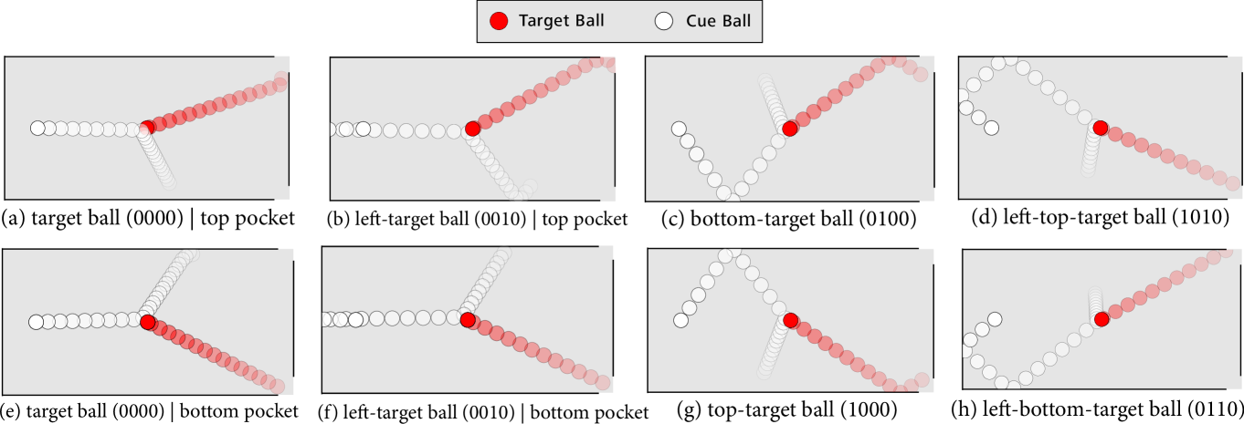
Figure 3: Sample solutions obtained from running STAMP on the billiards problem. The sub-captions indicate which walls are hit by the cue ball before hitting the target ball. That is, the first, second, third, and fourth digit correspond to hitting the top, bottom, left, and right wall, respectively. A 1 means that the wall is hit during the shot, a 0 means that it is not. The caption also indicates in which pocket the target ball is shot.

Our method, Stein TAMP (STAMP), solves for diverse task and motion plans by approaching TAMP as a joint Bayesian inference problem over discrete variables (symbolic plans) and continuous variables (geometric plans). Stein Task and Motion Planning (STAMP) begins by randomly initializing a set of candidate task and motion plans (‘particles’ or ‘samples’) and subsequently updates these via continuous and discrete SVGD. The goal of inference is to move these plans towards high density regions of a target distribution that effectively measures how optimal a plan is, based on their cost and constraints. After running inference, the plans are refined via stochastic gradient descent (SGD) to obtain exact optima in the target distribution. Formulating TAMP as a Bayesian inference problem allows us to sample optimal plans from various modes within the target distribution, which translates to finding a variety of optimal plans to a given TAMP problem. We illustrate our algorithm pipeline in Figure 2 and describe our approach in detail below.

IV-A TAMP as SVGD Inference

We first provide an analogy for STAMP in Figure 1, which illustrates using SVGD to run joint discrete-and-continuous inference on a simple Gaussian mixture. In this example, the goal is to move a set of particles towards high-density regions in the Gaussian mixture, while also ensuring that the particles obtain the correct class label post-inference. This involves inference over both discrete and continuous variables, as both the particles’ class labels and their positions must be learned. In STAMP, we similarly use SVGD to run discrete-and-continuous inference. The discrete class labels are analogous to the discrete symbolic plans, and the particles’ positions are analogous to the continuous geometric plans. The Gaussian mixture is analogous to a posterior distribution over the task and motion plan condition on the plan being optimal.

We now formalize our approach. Given a problem domain, we are interested in sampling optimal symbolic actions $\mathcal{A}_{1:K}\in\mathcal{Z}^{K}$ and controls $u_{0:KT-1}\in\mathbb{R}^{KT}$ from the posterior

$$p(\mathcal{A}_{1:K},u_{0:KT-1}\mid O=1)$$ (8)

where $O\in\{0,1\}$ indicates optimality of the plan; $K$ the number of symbolic action sequences; $T$ is the number of timesteps by which we discretize each action sequence; and $\mathcal{Z}$ is a discrete set of all $m$ possible symbolic actions that can be executed in the domain (i.e., $|\mathcal{Z}|=m$). $\mathcal{A}_{1:K}$ and $u_{0:KT-1}$ fully parameterize a task and motion plan, since they can be inputted to a physics simulator $f_{\text{sim}}$ along with the initial state $x_{0}$ to roll out states at every timestep, that is, $x_{1:KT}=f_{\text{sim}}(x_{0},\mathcal{A}_{1:K},u_{0:KT-1})$.

We use SVGD to sample optimal plans from $p(\mathcal{A}_{1:K},u_{0:KT-1}\mid O=1)$. As $p$ is defined over both continuous and discrete domains, to use SVGD’s gradient-based update rule, we follow [9]’s approach of relaxing the discrete variables to the continuous domain by constructing a map from the real domain to $\mathcal{Z}^{K}$ that evenly partitions some base distribution $p_{0}$. For any problem domain with $m$ symbolic actions, we propose defining $\mathcal{Z}=\{e_{i}\}_{i=1}^{m}$ as a collection of $m$-dimensional one-hot vectors. Then, $\mathcal{A}_{1:K}\in\mathcal{Z}^{K}$, implying that we commit to one action ($e_{i}$) in each of the $K$ action phases. Further, we propose using a uniform distribution for the base distribution $p_{0}$. Given this formulation, we can define a map $\Gamma:\mathbb{R}^{mK}\rightarrow\mathcal{Z}^{K}$ and its differentiable surrogate $\tilde{\Gamma}$ as the following (note, $x\in\mathbb{R}^{mK}$):

$$\Gamma(x) =[\max\bigl{\{}x_{1:m}\bigr{\}}\ldots\max\bigl{\{}x_{(K-1)m+1:mK}\bigr{\}}]^{\top}$$ (9)

$$\tilde{\Gamma}(x) =[\text{softmax}\bigl{\{}x_{1:m}\bigr{\}}\ldots\text{softmax}\bigl{\{}x_{(K-1)m+1:mK}\bigr{\}}]^{\top}.$$ (10)

We show in Appendix A that the above map indeed partitions $p_{0}$ evenly when $p_{0}$ is the uniform distribution.

Our relaxation of $\mathcal{A}_{1:K}$ allows us to run inference over purely continuous variables: $a_{1:K}\in\mathbb{R}^{mK}$ and $u_{0:KT-1}\in\mathbb{R}^{KT-1}$, where $\mathcal{A}_{1:K}=\Gamma(a_{1:K})$. We denote these variables as $\theta=[a_{1:K},u_{0:KT-1}]^{\top}$, and randomly initialize SVGD samples $\{\theta_{i}\}_{i=1}^{n}$ to run inference. The target distribution we aim to infer is a differentiable surrogate $\rho$ of $p$, which we define following equation (3) as:

$$\rho(a_{1:K},u_{0:KT-1}\mid O=1)$$ (11)

$$\propto p_{0}(a_{1:K})\,p(\tilde{\Gamma}(a_{1:K}),u_{0:KT-1}\mid O=1).$$ (12)

In practice, because SVGD requires $\nabla_{\theta}\log\rho$ for its updates and the gradient of $\log p_{0}$ is zero everywhere except at its boundary (which we can make arbitrarily large to avoid), we simply let

$$\rho(a_{1:K},u_{0:KT-1}\mid O=1)\propto p(\tilde{\Gamma}(a_{1:K}),u_{0:KT-1}\mid O=1).$$ (13)

Further, we note that it is not necessary to normalize the $\rho$ as the normalization constant vanishes by taking the gradient of $\log\rho$.

We now quantify the surrogate of the posterior distribution. We begin by applying Bayes’ rule and obtain the following factorization of $\rho(\theta\mid O=1)$:

$$\rho(a_{1:K},u_{0:KT-1}\mid O=1)$$ (14)

$$\propto\rho(O=1\mid a_{1:K},u_{0:KT-1})\,\rho(a_{1:K},u_{0:KT-1}).$$ (15)

We see that the likelihood function measures the optimality of a plan, and as such, we define it using the total cost $C$ associated with the task and motion plan:

$$\begin{gathered}p(O{=}1|a_{1:K},u_{0:KT-1})\propto\exp{-C(a_{1:K},u_{0:KT-1},x_{0:KT})}.\end{gathered}$$ (16)

Meanwhile, the prior $p(a_{1:K},u_{0:KT-1})$ is defined over $\theta$ only and as such, we use it to impose constraints on the plan parameters (e.g., kinematic constraints on robot joints). Our formulation closely follows the mathematical program description of LGP [4, 12, 13, 14, 15] which solves TAMP as a cost-minimization problem with multiple constraint functions. In our formulation, the total cost $C$ is designed as a weighted sum of the objective function and constraints (excluding those embedded into the prior). The objective function is typically defined as a loss on the final state $x_{KT}=f_{\text{sim}}(x_{0},a_{1:K},u_{0:KT-1})$ that penalizes large deviations from the desired goal state. Constraint functions can be defined to encode the robot’s kinematics and dynamics constraints, as well as constraints that enforce consistency between the trajectory and symbolic action variables.

Finally, we describe how we run inference over $\theta$ using SVGD as the inference algorithm. We first randomly initialize $n$ candidate task and motion plans $\{\theta_{i}\}_{i=1}^{n}$, and simulate each plan in parallel using Warp [10] as the differentiable physics simulator. This allows us to generate states $x_{0:KT}=f_{\text{sim}}(x_{0},\theta)$. Then, we compute the surrogate posterior distribution $\rho$ from equations (13), (15), and (16). We use Warp’s auto-differentiation capabilities to compute gradients of the log-posterior with respect to $\{\theta_{i}\}_{i=1}^{n}$ in parallel, and use these gradients to update each candidate plan $\theta_{i}$ via the update rule in equation (4). Since all of the above processes are parallelized on the GPU using Warp, each SVGD update is very efficient. We continue to update the plans until SVGD converges.

IV-B Plan Refinement via SGD

As an inference algorithm, SVGD will lead to few samples that converge exactly to optima in the posterior distribution. The repulsive force between the samples, $\nabla_{\theta}k(\theta,\theta^{\prime})$, encourages the particles to explore, leading to diverse plans, but can simultaneously push the plans away from optima. Since we are interested in finding a diverse set of exact solutions, we exploit both SVGD and SGD in our algorithm, which allows us to balance the trade-off between exploration and optimization. After running SVGD to obtain a distribution of plans that cover multiple modes in $\rho(a_{1:K},u_{0:KT-1}\mid O=1)$, we finetune the candidate plans with SGD to obtain optimal solutions. This approach of combining SVGD with SGD allows us to find a diverse set of optimal plans. The pseudocode for our complete optimization routine is shown in Algorithm 1.

IV-C Learning Action Abstractions

Long-horizon TAMP problems are of great interest to the robotics community. One way to more effectively solve long-horizon problems is to leverage action abstractions. In our framework, we leverage differentiable action abstractions to reduce TAMP to a lower-dimensional inference problem. This results in more effective inference as the repulsive term in the SVGD update rule negatively correlates with the particle dimensionality [33, 34]. For STAMP, the controls $u_{0:KT-1}$ are the primary cause of high-dimensionality, particularly as the planning horizon increases (which can occur if the number of action sequences $K$ and/or the number of timesteps $T$ is increased).

To tackle this, we use imitation learning to create low-dimensional abstractions for $u_{0:KT-1}$, which significantly reduces the dimensionality of our inference problem. Our idea is to create a bank of goal-conditioned dynamic motion primitives (DMP) from demonstration data, whose weights we train offline. We train one DMP, or skill, for every possible action. Once trained, we use the DMP s to generate trajectories $\hat{x}_{kT:(k+1)T}$ given the desired goal pose ${g}_{k}$ for each action sequence $a_{k}$. Then, we obtain the controls $u_{0:KT-1}$ using a differentiable controller that tracks $\hat{x}_{0:KT}$. This approach effectively reduces the problem from finding all of $u_{0:KT-1}\in\mathbb{R}^{KT}$ to finding $g_{1:K}\in\mathbb{R}^{Kd}$, where $d\ll T$ are the degrees of freedom of the system.

Besides dimensionality reduction, the main benefits of DMPs are that they are differentiable (a requirement of STAMP), ensure smooth trajectories $\hat{x}_{k:(k+t)T}$, and guarantee convergence to the desired goal in each segment.

V Evaluation

Table I: Runtime Comparison between STAMP and Baselines

Method	Time / Solution ($\mathrm{s}$)	Runtime ($\mathrm{s}$)
Billiards
Diverse LGP	(38.1$\pm$8.7)	(38.1$\pm$8.7)
PDDLStream	(5.7$\pm$.8)	(5.7$\pm$.8)
STAMP (Ours)	(0.068$\pm$0.007)	(6.94$\pm$.06)
Pusher (maximum 2 pushes)
Diverse LGP	(15.6$\pm$2.9)	(15.6$\pm$2.9)
PDDLStream*	(22.2$\pm$.1)	(110.9$\pm$.7)
STAMP (Ours)	(0.0157$\pm$.0004)	(12.92$\pm$.04)

• Averaged across $10$ seeds; STAMP is initialized with 1100 particles.

• * Modified to enable diverse planning.

Table II: Runtime of STAMP Varying the Number of Particles

Particle Count	Billiards ($\mathrm{s}$)	Block-Pushing ($\mathrm{s}$)
700	(6.30$\pm$.07)	(12.53$\pm$.05)
900	(6.55$\pm$.04)	(12.74$\pm$.03)
1100	(6.94$\pm$.06)	(12.92$\pm$.04)
1300	(7.71$\pm$.12)	(13.22$\pm$.06)

• Averaged across $10$ seeds; maximum of 2 pushes.

Table III: Runtime of STAMP Varying the Particle Dimensionality for Block-Pushing

Max. Push Count	Dimensionality	Runtime ($\mathrm{s}$)
2	16	(12.92$\pm$.04)
3	24	(12.93$\pm$.04)
4	32	(13.26$\pm$.03)
5	40	(13.57$\pm$.03)

• Averaged across $10$ seeds; STAMP is initialized with 1100 particles.

We demonstrate the effectiveness of STAMP by solving two problems requiring discrete-and-continuous planning: billiards and block-pushing. We describe these problem environments and our algorithmic setup in Section V-A below. We benchmark our algorithm against two TAMP baselines that build upon PDDLStream [3] and Diverse LGP [35], whose implementation we detail in Appendix E. In our experiments, we aim to answer the following questions:

1. Can STAMP return a variety of accurate plans for TAMP problems for which multiple solutions are possible?

2. Does STAMP conduct a more time-efficient search over symbolic and geometric plans compared to existing baselines?

3. How does the computational time of TAMP scale with respect to the dimensionality of the problem and the number of samples used during inference?

V-A Problem Environments and Their Algorithmic Setup

Figure 4: Distribution of plans found by STAMP (our method), Diverse LGP, and PDDLStream on the block-pushing problem (with max. two pushes). Diverse LGP and PDDLStream are invoked as many times as STAMP found solutions. Results are averaged across $10$ seeds; the error bars represent the standard deviation.

Figure 5: Distribution of plans found by STAMP (our method), Diverse LGP, and PDDLStream on the billiards problem. Diverse LGP and PDDLStream are invoked as many times as STAMP found solutions. Results are averaged across $10$ seeds; the error bars represent the standard deviation.

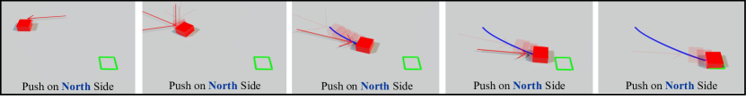
(a) Push on north side.

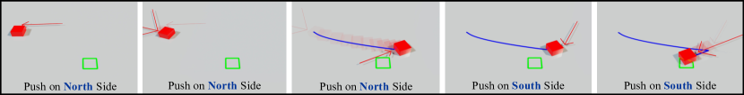
(b) Push on north side, followed by push on south side.

Figure 6: Sample solutions obtained from running STAMP on the block pushing problem. The red arrow is proportional to the magnitude and direction of the pushing force, the blue line shows the block’s trajectory, and the green box shows the goal region.

V-A1 Billiards

We aim to find multiple ways of hitting the target ball with the cue ball such that the target ball ends up in one of the two pockets on the right side of Figure 7 in Appendix B (see Figure 3 for a variety of different solutions to this problem). This involves symbolic planning as we must plan which walls the cue ball should bounce off of before making contact with the target ball. It also involves continuous “motion planning” as we must find the initial velocity $u_{0}=[v_{x},v_{y}]^{\top}$ to inflict on the cue ball such that the target ball ends up in one of the pockets. We use STAMP to optimize $u_{0}$ and the task plan $\mathcal{A}=[z_{1},z_{2},z_{3},z_{4}]\in\{0,1\}^{4}$, which indicates which of the four walls the cue ball bounces off of. $z_{i}=1$ if the cue ball bounces off of wall $i$, and it is $0$ otherwise. We label each wall using numbers 1-4 in Figure 7 in Appendix B. In practice, we show that we can relax $\mathcal{A}\in\{0,1\}^{4}$ into $a=[w_{1},w_{2},w_{3},w_{4}]\in[0,1]^{4}$ and express $a$ as a function of $u_{0}$ (see Appendix B-B). Since $a$ is a function of $u_{0}$, we simply define our SVGD samples as $\theta=[u_{0}]^{\top}$ as optimizing $u_{0}$ will implicitly optimize $a$. To encourage diversity in the logical plans, we employ $a$ along with $u_{0}$ within the kernel. We refer the reader to Appendix B-C for details on how the kernel is defined for this problem.

To construct the target distribution $\rho(\theta\mid O=1)$, we employ expressions (15) and (16). Our cost function $C$ is a weighted sum of the target loss $L_{\text{target}}$ and aim loss $L_{\text{aim}}$, with hyperparameters $\beta_{\text{target}}$ and $\beta_{\text{aim}}$ as the respective coefficients:

$$C(\theta)=\beta_{\text{aim}}L_{\text{aim}}+\beta_{\text{target}}L_{\text{target}}$$ (17)

The target loss is minimal when the cue ball ends up in either of the two pockets, whereas the aim loss is minimal if the cue ball comes in contact with the target ball at any point in its trajectory. We define these loss terms in Appendix B-D.

V-A2 Block-Pushing

Our goal is to push the block in Figure 8 in Appendix C towards the goal region. We wish to plan symbolic actions consisting of which side of the block–-north, east, south, or west–-we push against; we associate each with numbers $1,...,4$ as shown in Figure 8 in Appendix C. We also wish to find the forces and the block’s trajectory at every time-step. For simplicity, we assume up to $K$ action sequences can be committed a priori. We reduce the dimensionality of the motion planning problem by parameterizing the motion plan by a series of $K$ intermediate goal poses $g_{x,y,\phi}^{(1:K)}\in\mathbb{R}^{3K}$, and rely on a library of DMP s, a controller, and the simulator to generate the trajectory, forces, and rolled-out states from $g_{x,y,\phi}^{(1:K)}$.

We define our samples as

$$\theta=\Bigl{[}s_{1:4}^{(1)},\dots,s_{1:4}^{(K)},g_{x,y,\phi}^{(1)},\dots,g_{x,y,\phi}^{(K)}\Bigr{]}^{\top}.$$ (18)

The task plan for the $k\/$th action is $a_{k}=s_{1:4}^{(k)}\in\mathbb{R}^{4}$, which maps to a one-hot encoding $e_{i}$, $i=1,...,4$ that determines which of the four sides to push on. We define the map from $\mathbb{R}^{4}$ to $e_{i}$ to be $\Gamma\bigl{(}s_{1:4}^{(k)}\bigr{)}=\max\bigl{\{}s_{1:4}^{(k)}\bigr{\}}$. The corresponding relaxed map is $\tilde{\Gamma}\bigl{(}s_{1:4}^{(k)}\bigr{)}=\text{softmax}\bigl{\{}s_{1:4}^{(k)}\bigr{\}}$, which can be differentiated with respect to $s_{1:4}^{(k)}$ for DSVGD updates. Our base distribution $p_{0}(\theta)$ is the uniform distribution. We define a positive-definite kernel for $\theta$ in Appendix C-B that operates on the task and motion plans separately and accounts for angle wrap-around for $g_{\phi}^{(1:K)}$.

We formulate the target distribution by defining the cost as a weighted sum of the target loss $L_{\text{target}}$ and trajectory loss $L_{\text{trajectory}}$. The target loss penalizes large distances between the cube and the goal region at the final time-step $KT$. The trajectory loss is a function of the intermediate goals $g_{x,y}^{(1:K)}$ and penalizes the pursuit of indirect paths to the goal. Since $L_{\text{trajectory}}$ is only a function of $g_{x,y}^{(1:K)}$, it places a prior on $g_{x,y}^{(1:K)}$, whereas $L_{\text{target}}$ makes up the likelihood function. In summary, our target distribution is the following.

$$p(\theta\mid O=1) \propto\exp{-C(\theta,x_{0:KT})}$$ (19)

$$=\exp{-\beta_{\text{target}}L_{\text{target}}(x_{KT})}$$

$$\quad\times\exp{-\beta_{\text{trajectory}}L_{\text{trajectory}}(g_{x,y}^{(1:K)})}$$

Appendix C-C describes this in greater detail.

V-B Experimental Results

V-B1 Solution Variety (Q1)

Invoking STAMP once, we find multiple distinct plans to both problems. These plans have diverse coverage not only in terms of the types of symbolic plans found, but also the motion plans associated with each symbolic plan. STAMP’s ability to generate diverse task plans is shown in Figures 4 and 5, which are histograms enumerating the number of (accurate, i.e., “good”) plans found for each task plan; our results cover a broad spectrum of task plans for both problems. Figures 3 and 6 show example solutions our method found. Our experiments also show that STAMP is capable of intra-task diversity; that is, it can find multiple motion plans that accomplish the same symbolic action. For instance, in Figure 3, we see that our method found two distinct initial cue ball velocities that accomplish the task plan “0000” (i.e., a direct hit). Our observations are consistent with the intuition that the repulsive term in SVGD encourages diversity in both task and motion plans.

V-B2 Baseline Comparison (Q2)

Table I shows that STAMP is able to find the same number of solutions in substantially less time than the Diverse LGP and PDDLStream baselines for both environments. Whereas STAMP optimizes over hundreds of possible action sequences in parallel, both baselines attempt to generate a single plan in succession. Although search-based symbolic planners, like in PDDLStream, may be more efficient for determining a single solution, the ability of STAMP to reduce the time needed for motion planning becomes critical for generating multiple solutions. This distinction is apparent in the billiards problem, in which all methods use SGD to plan initial velocities but STAMP is several factors faster than the baselines. Further, STAMP learns a distribution over possible solutions, meaning the resulting modes are inherently more likely and tractable. In contrast, because diversity is forced into LGP and PDDLStream through methods like blocking or randomly selecting actions, both baselines will often consider difficult modes and be subject to the lengthy solving times needed for such modes.

V-B3 Scalability to Higher Dimensions and Greater Number of Samples (Q3)

Tables II and III show the total runtime of our algorithm while varying the number of samples and particle dimensions. They show that increasing the number of samples and the dimensions of the particles has little effect on the total optimization time required by STAMP. This is unsurprising as STAMP is parallelized over the number of samples and dimensions, made possible through the use of Warp and SVGD, both of which are parallelizable. Further, this result indicates that STAMP has the potential to efficiently solve long-horizon TAMP problems, which would require a greater number of samples and higher-dimensional inference. This is because long-horizon problems involve longer action sequences and naturally have highly multimodal posterior distributions due to the multitude of solutions possible, so a large number of samples would be required to run effective inference.

VI Conclusion

We introduced STAMP, a novel algorithm for solving TAMP problems that makes use of parallelized Stein variational gradient descent and differentiable physics simulation. In our algorithm, we formulated TAMP as a variational inference problem over discrete symbolic actions and continuous motions, and validated our approach on the billiards and block-pushing TAMP problems. Our method was able to discover a diverse set of plans covering multiple different task sequences and also a variety of motion plans for the same task plan. Critically, we also showed that STAMP, through exploiting parallel gradient computation from a differentiable simulator, is much faster at finding a variety of solutions than popular TAMP solvers, and scales well to higher dimensions and more samples. In future work, we aim to test our method on more challenging TAMP problems, particularly problems that involve long-horizon planning and multiple constraints.

Appendix A Relaxations for Discrete SVGD

Given a problem domain with $m$ possible actions, the goal of TAMP is to find a $K$-length sequence of symbolic actions $\mathcal{A}_{1:K}\in{Z}^{K}$ and associated motions that solve some goal. Here, $\mathcal{Z}$ is a discrete set of $m$ possible symbolic actions in the domain. We propose the general formulation of $\mathcal{Z}$ as the set of $m$-dimensional one-hot encodings such that $|\mathcal{Z}|=m$ and $|\mathcal{Z}^{K}|=m^{K}$. Then, as per equation (2), we can simply relax $\mathcal{A}_{1:K}\in{Z}^{K}$ to the real domain $\mathbb{R}^{mK}$ by constructing the map $\Gamma:\mathbb{R}^{mK}\rightarrow\mathcal{Z}^{K}$ as

$$\Gamma(x)=\begin{bmatrix}\text{max}\bigl{\{}x_{1:m}\bigr{\}}\\ \text{max}\bigl{\{}x_{m+1:2m}\bigr{\}}\\ \vdots\\ \text{max}\bigl{\{}x_{(K-1)m+1:mK}\bigr{\}}\end{bmatrix}$$ (20)

and its differentiable surrogate as

$$\tilde{\Gamma}(\cdot)=\begin{bmatrix}\text{softmax}\bigl{\{}x_{1:m}\bigr{\}}\\ \text{softmax}\bigl{\{}x_{m+1:2m})\bigr{\}}\\ \vdots\\ \text{softmax}\bigl{\{}x_{(K-1)m+1:mK}\bigr{\}}\end{bmatrix}.$$ (21)

We will prove that the above mapping evenly partitions $\mathbb{R}^{mK}$ into $m^{K}$ parts when the base distribution $p_{0}$ is a uniform distribution over $[-u,u]^{mK}$ for some $u>0$. We will prove this in two steps: firstly by assuming $K=1$ and then proving this for any positive integer $K$.

A-A The Base Distribution

Our base distribution $p_{0}(x),x\in\mathbb{R}^{mK}$ for discrete SVGD is a uniform distribution over the domain $[-u,u]^{mK}$. That is,

$$p_{0}(x)=\text{unif}(x)\\ =\begin{cases}\frac{1}{{(2u)}^{mK}}&\text{if }x\in[-u,u]^{mK}\\ 0&\text{otherwise}.\end{cases}$$ (22)

Note that in practice, we can make $u\in(0,\infty)$ arbitrarily large to avoid taking gradients of $p_{0}$ at the boundaries of $[-u,u]^{K}$.

A-B Proof of Even Partitioning: Case $K=1$

To satisfy the condition that $\Gamma(x),x\in\mathbb{R}^{m}$ evenly partitions $\text{unif}(x)$, for all $\{e_{i}\}_{i=1}^{m}\in\mathcal{Z}$, the following must be true.

$$\int_{\mathbb{R}^{m}}\text{unif}(x)\mathbb{I}[e_{i}=\Gamma(x)]\,\mathrm{d}x=\frac{1}{m}$$ (23)

Below, we show that the left hand side (LHS) of the above equation simplifies to $\frac{1}{m}$, proving that our relaxation evenly partitions $p_{0}(\cdot)$.

LHS $$=\int_{\mathbb{R}^{m}}\text{unif}(x)\mathbb{I}[e_{i}=\text{max}(x)]\,\mathrm{d}x$$ (24)

$$=\frac{1}{{(2u)}^{m}}\int_{-u}^{u}\ldots\int_{-u}^{u}\mathbb{I}[e_{i}=\text{max}(x)]\,\mathrm{d}x_{1}\ldots\mathrm{d}x_{m}$$ (25)

$$=\frac{1}{{(2u)}^{m}}\int_{-u}^{u}\ldots\int_{-u}^{u}\prod_{j=i,j\neq 1}^{m}\mathbb{I}[x_{i}>x_{j}]\,\mathrm{d}x_{1}\ldots\mathrm{d}x_{m}$$ (26)

$$=\frac{1}{{(2u)}^{m}}\int_{-u}^{u}\Bigg{(}\prod_{j=i,j\neq 1}^{m}\int_{-u}^{x_{i}}\mathbb{I}[x_{i}>x_{j}]\,\mathrm{d}x_{j}\Bigg{)}\,\mathrm{d}x_{i}$$ (27)

$$=\frac{1}{{(2u)}^{m}}\int_{-u}^{u}\Bigg{(}\prod_{j=i,j\neq 1}^{m}\int_{-u}^{x_{i}}\,\mathrm{d}x_{j}\Bigg{)}\,\mathrm{d}x_{i}$$ (28)

$$=\frac{1}{{(2u)}^{m}}\int_{-u}^{u}\Bigg{(}\int_{-u}^{x_{i}}\,\mathrm{d}y\Bigg{)}^{m-1}\,\mathrm{d}x_{i}$$ (29)

$$=\frac{1}{{(2u)}^{m}}\int_{-u}^{u}(x_{i}+u)^{m-1}\,\mathrm{d}x_{i}$$ (30)

$$=\frac{1}{({2u})^{m}}\cdot\frac{(2u)^{m}}{m}$$ (31)

$$=\frac{1}{m}$$ (32)

∎

A-C Proof of Even Partitioning: Case $K>1$

For $\Gamma(x)$ to evenly partition $\text{unif}(x),x\in\mathbb{R}^{mK}$, the following must be true for all $\{z_{i}\}_{i=1}^{m^{K}}\in\mathcal{Z}^{K}$.

$$\int_{\mathbb{R}^{mK}}\text{unif}(x)\mathbb{I}[z_{i}=\Gamma(x)]\,\mathrm{d}x=\frac{1}{m^{K}}$$ (33)

We use the results from Appendices A-A and A-B to show that the left hand side of the above equation simplifies to $\frac{1}{m^{K}}$, proving that our relaxation evenly partitions $p_{0}(\cdot)$. Below, we use the following notation: $\mathbf{u}=[u\ldots u]\in\mathbb{R}^{m}$, $(z_{i})_{k}$ is the $k$th $m$-dimensional one-hot vector within $z_{i}\in\mathcal{Z}^{K}$, and $\mathbf{x}_{k}=x_{(k-1)m+1:km}\in\mathbb{R}^{m}$.

LHS $$=\int_{\mathbb{R}^{mK}}\text{unif}(x)\prod_{k=1}^{K}\mathbb{I}[(z_{i})_{k}=\text{max}(\mathbf{x}_{k})]\,\mathrm{d}x$$ (34)

$$=\frac{1}{(2u)^{mK}}\prod_{k=1}^{K}\int_{-\mathbf{u}}^{\mathbf{u}}\mathbb{I}[(z_{i})_{k}=\text{max}(\mathbf{x}_{k})]\,\mathrm{d}\mathbf{x}_{k}$$ (35)

$$=\frac{1}{(2u)^{mK}}\prod_{k=1}^{K}\frac{(2u)^{m}}{m}$$ (36)

$$=\frac{1}{(2u)^{mK}}\cdot\frac{(2u)^{mK}}{m^{K}}$$ (37)

$$=\frac{1}{m^{K}}$$ (38)

∎

Appendix B Billiards Problem Setup

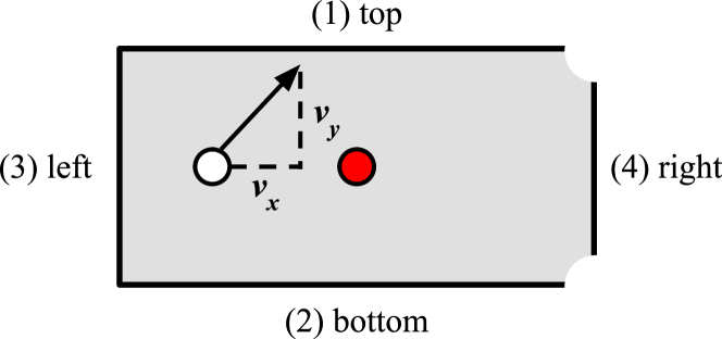
Figure 7: Graphical depiction of the billiards problem environment. The goal is to shoot the target ball (red) into one of the pockets on the right by finding an initial velocity for the cue ball (white). The task plan is give by the wall(s) the cue ball should hit before hitting the target ball.

B-A Graphical Overview

A graphical depiction of the billiards problem environment is shown in Figure 7. We recreate this environment in the Warp simulator.

B-B Task Variables as Functions of Velocity

We show here that the task variable $a=w_{1:4}$ can be formulated as a soft function of the initial cue ball velocity $u_{0}=(v_{x},v_{y})$. To do so, we first simulate the cue ball’s trajectory in a differentiable physics simulator, given the initial cue ball velocity $u_{0}=[v_{x},v_{y}]$. We then use the rolled-out trajectory of the cue ball $x_{1:T}^{\text{cue}}$ to define a notion of distance at time $t$ between the cue ball and wall $i$ as follows.

$$d_{t}^{\text{wall-cue}}=-\alpha\text{ SignedDistance}(x_{t}^{\text{cue}},\text{wall}_{i})+\beta$$ (39)

In the above, $\alpha>0,\beta\in\mathbb{R}$ are hyperparameters that can be tuned to scale and shift the resulting value.

Then, we use $d_{t}^{\text{wall-cue}}$ to formulate the task variable $w_{1:4}$ as a soft function of $u_{0}$ as follows.

$$w_{i} =\frac{1}{1+\exp{-d_{\text{weighted}}}},$$ (40)

$$d_{\text{weighted}} =\sum_{t=1}^{t_{c}}\sigma_{t}d_{t}^{\text{wall-cue}},$$ (41)

$$\sigma_{t} =\frac{\exp{d_{t}^{\text{wall-cue}}}}{\sum_{k=1}^{t_{c}}\exp{d_{k}^{\text{wall-cue}}}}$$ (42)

Although $w_{i}$ is not directly related to $u_{0}$, we note that both quantities are related implicitly since $d_{t}^{\text{wall-cue}}$ is a function of $x_{t}^{\text{cue}}$, which result from simulating the cube ball forward using $u_{0}$ as the initial ball velocity.

We note that the above formulation of $w_{i}$ gives us the binary behavior we want for the task variable, but in a relaxed way. That is, $w_{i}$ will either take on a value close to 1 or close to 0. Intuitively, the sigmoid function will assign a value close to $1$ to $w_{i}$ if the negative signed distance between the wall $i$ and the cue ball is large at some point in the cue ball’s trajectory up until $t_{c}$, which is the time of contact with the target ball. This can only occur if the cue ball hits wall $i$ at some point in its trajectory before time $t_{c}$. Conversely, if the cue ball remains far from wall $i$ at every time step up to $t_{c}$, $w_{i}$ will correctly evaluate to a value close to 0. Note that $\alpha$ and $\beta$ can be tuned to get the behavior we want for $w_{i}$.

Critically, we note that the above formulation is differentiable with respect to $u_{0}$. By relaxing $w_{i}$ using a sigmoid function over $d_{\text{weighted}}$ and using a differentiable physics simulator to roll out the cue ball’s trajectory, we effectively construct $w_{i}$ as soft and differentiable functions of $u_{0}$. The differentiability of $w_{i}$ with respect to $u_{0}$ is important; because of the way we formulate the kernel (see Appendix B-C), the repulsive force $\nabla_{\theta}k(\theta,\theta^{\prime})$ in the SVGD update requires gradients of $w_{i}$ with respect to $u_{0}$ via the chain rule.

B-C Kernel Definition

We build upon the Radial Basis Function (RBF) kernel, a popular choice in the SVGD literature, to design a positive definite kernel for $\theta=[v_{x},v_{y}]^{\top}$. Whereas RBF kernels operate over $\theta$, we operate the RBF kernel over $[\theta,w_{1:4}(\theta)]^{\top}$, and tune separate kernel bandwidths for $v_{x,y}$ and $w_{1:4}(v_{x,y})$, which we denote as $s_{v_{x,y}}$ and $s_{w_{1:4}}$, respectively. This is to account for differences in their range. We use the median heuristic [36] to tune the kernel bandwidths.

$$k(\theta,\theta^{\prime})=\exp{-\frac{\bigl{\lVert}\theta-\theta^{\prime}\bigr{\rVert}_{2}^{2}}{s_{v_{x,y}}^{2}}-\frac{\bigl{\lVert}w_{1:4}(\theta)-w_{1:4}(\theta^{\prime})\bigr{\rVert}_{2}^{2}}{s_{w_{1:4}}^{2}}}$$ (43)

B-D Loss Definitions

We define the target and aim loss for the billiards problem below. Given the final state at time $T$ of the target ball $x_{T}^{\text{target}}$, the position of the top pocket $g_{\text{top}}$, the position of the bottom pocket $g_{\text{bottom}}$, and the radius $R$ of the balls, the target loss is defined as the following.

$$L_{\text{target}}=\min(\lVert x_{T}^{\text{target}}-g_{\text{top}}\rVert_{2}^{2},\lVert x_{T}^{\text{target}}-g_{\text{bottom}}\rVert_{2}^{2})$$ (44)

To define the aim loss, we first introduce the time-stamped aim loss $L_{\text{aim}}^{(t)}$ which is equal to the distance between the closest points on the surface of the target ball and the surface of the cue ball at time $t$:

$$L_{\text{aim}}^{(t)}=\max(0,\absolutevalue{x_{t}^{\text{target}}-x_{t}^{\text{cue}}}-2R)$$ (45)

The aim loss $L_{\text{aim}}$ is the softmin-weighted sum of the time-stamped aim loss throughout the cue ball’s time-discretized trajectory up until time $t_{c}$, which is the time of first contact with the target ball.

$$L_{\text{aim}} =\sum_{t=1}^{t_{c}}\sigma_{t}L_{\text{aim}}^{(t)}, \sigma_{k} =\frac{\exp{-L_{\text{aim}}^{(k)}}}{\sum_{t=1}^{t_{c}}\exp{-L_{\text{aim}}^{(t)}}}$$ (46)

Appendix C Block-Pushing Problem Setup

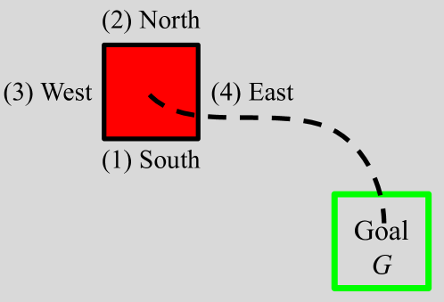
Figure 8: Graphical depiction of the block-pushing problem environment. The goal is to push the red block into the green goal region by repeatedly applying pushes to either north, south, west, or east of the red block. The task plan is given by the side(s) to push from.

C-A Graphical Overview

Figure 8 shows a graphical overview of the block-pushing problem environment, which we recreate in the Warp simulator.

C-B Kernel Definition

We employ the additive property of kernels to construct our positive-definite kernel. The kernel is a weighted sum of the RBF kernel over $\{g_{x,y}^{(k)}\}_{k=1}^{K}$, the RBF kernel over $\{\text{softmax}(s_{1:4}^{(k)})\}_{k=1}^{K}$, and the von Mises kernel over $\{g_{\phi}^{(k)}\}_{k=1}^{K}$. The von Mises kernel is a positive definite kernel designed to handle angle wrap-around.

$$K(\theta,\theta^{\prime}) =\sum_{k=1}^{K}\Bigl{[}\alpha_{g_{x,y}}K_{\text{RBF}}\Bigl{(}g_{x,y}^{(k)},g_{x,y}^{(k)^{\prime}}\Bigr{)}$$ (47)

$$\qquad+\alpha_{s_{1:4}}K_{\text{RBF}}\Bigl{(}\operatorname{softmax}\bigl{(}s_{1:4}^{(k)}\bigr{)},\operatorname{softmax}\Bigl{(}s_{1:4}^{(k)^{\prime}}\Bigr{)}\Bigr{)}$$

$$\qquad+\alpha_{g_{\phi}}K_{\text{VM}}\Bigl{(}g_{\phi}^{(k)},g_{\phi}^{(k)^{\prime}}\Bigr{)}\Bigr{]}$$

C-C Formulation of the Posterior Distribution

Our target distribution is the product of a prior $p\big{(}g_{x,y}^{(1:K)}\big{)}$ over the intermediate goals and the likelihood distribution $p(O=1\mid\theta)$. The prior relates to the trajectory loss $L_{\text{trajectory}}$ via the relationship $p(g_{x,y}^{(1:K)})\propto\exp(-\beta_{\text{trajectory}}L_{\text{trajectory}})$. The trajectory loss penalizes indirect trajectories towards the goal, and we formulate it using the Manhattan distance $D_{\text{MH}}$ and use the convention $g_{x,y}^{(0)}=x_{0}^{\text{cube}}$ to denote the cube’s starting state.

$$p\big{(}g_{x,y}^{(1:K)}\big{)} =\prod_{k=1}^{K}p\big{(}g_{x,y}^{(k)}\mid g_{x,y}^{(k-1)}\big{)}$$ (48)

$$p\big{(}g_{x,y}^{(k)}\mid g_{x,y}^{(k-1)}\big{)} \propto$$

The likelihood distribution relates to the target loss $L_{\text{target}}$, which measures the proximity of the cube to the goal at the end of simulation. We define the likelihood as $\exp(-\beta_{\text{target}}L_{\text{target}})$ where the target loss is defined to be the following.

$$L_{\text{target}}=\max\big{(}0,\absolutevalue{x_{T}^{\text{block}}-g_{x}}-t\big{)}^{2}+\max\big{(}0,\absolutevalue{x_{T}^{\text{block}}-g_{y}}\big{)}^{2}$$ (49)

C-D Further Results

Figure 6 shows sample solutions obtained from running STAMP on the block pushing problem.

Appendix D STAMP Optimization

Figure 9 shows how the particles move through the loss landscape of the billiards problem. Figure 10 shows how the loss evolves over various iterations of STAMP for the billiards and block-pushing problems.

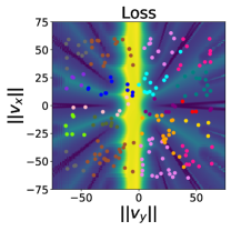
(a) Particles at initialization

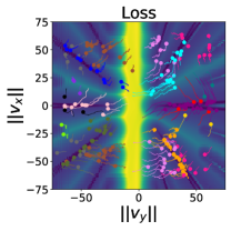
(b) Particles after SVGD inference

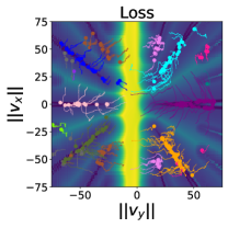
(c) Particles after SGD refinement

Figure 9: From left to right: evolution of the distribution of plan parameters $\theta$. On the left, $\theta$ are initialized uniformly, while in the middle, they converge to the full likelihood distribution post-SVGD. On the right, the particles collapse to the optima post-SGD. The particles’ colors indicate their mode (wall hits).

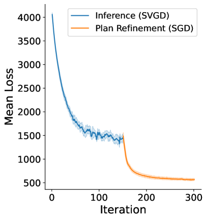
(a) Billiards

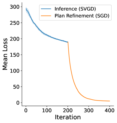
(b) Block-Pushing ($K=2$)

Figure 10: Evolution of mean loss over SVGD and SGD iterations.

Appendix E Implementation of Baselines

For both baselines, the logical or task plan is the walls to hit for the billiards problem and the sequence of sides to push from for the block pushing problem.

E-A PDDLStream

PDDLStream combines search-based classical planners with streams, which construct optimistic objects for the task planner to form an optimistic plan and then conditionally sample continuous values to determine whether these optimistic objects can be satisfied [3]. Since it is possible to create an infinite amount of streams and thus optimistic objects, the number of stream evaluations required to satisfy a plan is limited and incremented iteratively. As a result, PDDLStream will always return the first-found plan with the smallest possible sequence of actions in our evaluation problems, resulting in no diversity.

To generate different solutions, we force PDDLStream to select different task plans based on some preliminary work in https://github.com/caelan/pddlstream/tree/diverse. For the billiards problem, we can reduce the task planning problem by enumerating all possible wall hits and denoting each sequence as a single task, since the motion planning stream is only needed once for any sequence of wall hits. Then, we select a task by uniform sampling and try to satisfy it by sampling initial velocities that match the desired wall hits using SGD and Warp. For the block-pushing problem, we use a top-k or diverse PDDL planner to generate multiple optimistic plans of varying complexity. We then construct the problem environment with the same tools used in PDDLStream examples [3]: first making a simulation environment in PyBullet [37], calling pose samplers and a PyBullet motion planner package [38], then attempting to track the path with a PD force controller within a stream evaluation. Note that the distribution of solutions is highly dependent on the time allocated for sampling streams. Of the feasible candidate plans, PDDLStream randomly selects a solution.

E-B Logic-Geometric Programming

Diverse LGP [35] uses a two-stage optimization approach by first formulating the problem on a high, task-based, level (as an SAS⁺ [39] task). Subsequently, a geometric (motion planning) problem is solved conditioned on the logical plan. That is, the performed motion is required to fulfill the logical plan. A logical plan is called geometrically infeasible if there is no motion plan fulfilling it. Diverse LGP speeds up exploration by eagerly forbidding geometrically infeasible plan prefixes (for instance, if moving through a wall is geometrically infeasible, no sequence starting with moving through a wall has to be tested for geometric feasibility).

We use the first iteration of LAMA [40] (implemented as part of the Fast Downward framework [41]) as suggested by [35] [35] and use SGD for motion planning. To enforce diversity in the logical planner, we iteratively generate $25$ logical plans by blocking ones we already found. As Diverse LGP finds exactly one solution to the TAMP problem per run, we invoke it as many times as STAMP found solutions to get the same sample size.

For both billiards and block-pushing, we use the SGD component described in Section IV-B. For billiards, we additionally add a loss term ensuring that the required walls are hit. For pusher, it suffices to fix the first $4K$ variables of (18), $s_{1:4}^{(1)},\dots,s_{1:4}^{(K)}$. That is, excluding them from the SGD update.

References

- [1] Caelan Reed Garrett et al. “Integrated task and motion planning” In Annual review of control, robotics, and autonomous systems 4 Annual Reviews, 2021, pp. 265–293
- [2] Leslie Pack Kaelbling and Tomás Lozano-Pérez “Hierarchical task and motion planning in the now” In 2011 IEEE International Conference on Robotics and Automation, 2011, pp. 1470–1477 IEEE
- [3] Caelan Reed Garrett, Tomás Lozano-Pérez and Leslie Pack Kaelbling “PDDLStream: Integrating Symbolic Planners and Blackbox Samplers via Optimistic Adaptive Planning” In ICAPS 30, 2020, pp. 440–448
- [4] Marc Toussaint, Kelsey Allen, Kevin Smith and Joshua Tenenbaum “Differentiable Physics and Stable Modes for Tool-Use and Manipulation Planning” In Robotics: Science and Systems XIV, 2018
- [5] Naman Shah et al. “Anytime integrated task and motion policies for stochastic environments” In 2020 IEEE International Conference on Robotics and Automation (ICRA), 2020, pp. 9285–9291 IEEE
- [6] Leslie Pack Kaelbling and Tomás Lozano-Pérez “Integrated task and motion planning in belief space” In The International Journal of Robotics Research 32.9-10 Sage Publications Sage UK: London, England, 2013, pp. 1194–1227
- [7] Huihui Guo et al. “Recent trends in task and motion planning for robotics: A Survey” In ACM Computing Surveys ACM New York, NY, 2023
- [8] Qiang Liu and Dilin Wang “Stein Variational Gradient Descent: A General Purpose Bayesian Inference Algorithm” In Advances in Neural Information Processing Systems 29 Curran Associates, Inc., 2016 URL: https://proceedings.neurips.cc/paper_files/paper/2016/file/b3ba8f1bee1238a2f37603d90b58898d-Paper.pdf
- [9] Jun Han et al. “Stein variational inference for discrete distributions” In International Conference on Artificial Intelligence and Statistics, 2020, pp. 4563–4572 PMLR
- [10] Miles Macklin “Warp: A High-performance Python Framework for GPU Simulation and Graphics” NVIDIA GPU Technology Conference (GTC), https://github.com/nvidia/warp, 2022
- [11] Constructions Aeronautiques et al. “PDDL—the planning domain definition language” In Technical Report, Tech. Rep., 1998
- [12] Danny Driess, Jung-Su Ha, Marc Toussaint and Russ Tedrake “Learning Models as Functionals of Signed-Distance Fields for Manipulation Planning” In Proceedings of the 5th Conference on Robot Learning 164, Proceedings of Machine Learning Research PMLR, 2022, pp. 245–255
- [13] Marc Toussaint, Jung-Su Ha and Danny Driess “Describing Physics ¡italic¿For¡/italic¿ Physical Reasoning: Force-Based Sequential Manipulation Planning” In IEEE Robotics and Automation Letters 5.4, 2020, pp. 6209–6216
- [14] Marc Toussaint “Logic-Geometric Programming: An Optimization-Based Approach to Combined Task and Motion Planning” In Twenty-Fourth International Joint Conference on Artificial Intelligence, 2015
- [15] Jung-Su Ha, Danny Driess and Marc Toussaint “A Probabilistic Framework for Constrained Manipulations and Task and Motion Planning under Uncertainty” In 2020 IEEE International Conference on Robotics and Automation (ICRA), 2020, pp. 6745–6751
- [16] J. Murthy et al. “gradSim: Differentiable simulation for system identification and visuomotor control” In International Conference on Learning Representations, 2021 URL: https://openreview.net/forum?id=c_E8kFWfhp0
- [17] Filipe Avila Belbute-Peres et al. “End-to-end differentiable physics for learning and control” In Adv. Neural Inf. Process. Syst. 31, 2018
- [18] Yi-Ling Qiao, Junbang Liang, Vladlen Koltun and Ming C Lin “Scalable differentiable physics for learning and control” In arXiv preprint arXiv:2007.02168, 2020
- [19] Keenon Werling et al. “Fast and Feature-Complete Differentiable Physics Engine for Articulated Rigid Bodies with Contact Constraints” In Robotics: Science and Systems XVII, 2021
- [20] Taylor A Howell et al. “Dojo: A differentiable simulator for robotics” In arXiv preprint arXiv:2203.00806 9, 2022
- [21] Eric Heiden et al. “Disect: A differentiable simulation engine for autonomous robotic cutting” In arXiv preprint arXiv:2105.12244, 2021
- [22] Jie Xu et al. “Accelerated policy learning with parallel differentiable simulation” In arXiv preprint arXiv:2204.07137, 2022
- [23] Eric Heiden et al. “Probabilistic Inference of Simulation Parameters via Parallel Differentiable Simulation” In 2022 International Conference on Robotics and Automation (ICRA), 2022, pp. 3638–3645 DOI: 10.1109/ICRA46639.2022.9812293
- [24] Alexander Lambert et al. “Stein variational model predictive control” In arXiv preprint arXiv:2011.07641, 2020
- [25] Jimmy Envall, Roi Poranne and Stelian Coros “Differentiable Task Assignment and Motion Planning”
- [26] Yaofeng Desmond Zhong, Jiequn Han and Georgia Olympia Brikis “Differentiable Physics Simulations with Contacts: Do They Have Correct Gradients wrt Position, Velocity and Control?” In arXiv preprint arXiv:2207.05060, 2022
- [27] C Daniel Freeman et al. “Brax—A Differentiable Physics Engine for Large Scale Rigid Body Simulation” In arXiv preprint arXiv:2106.13281, 2021
- [28] Yuanming Hu et al. “Difftaichi: Differentiable programming for physical simulation” In arXiv preprint arXiv:1910.00935, 2019
- [29] Peter Pastor, Heiko Hoffmann, Tamim Asfour and Stefan Schaal “Learning and generalization of motor skills by learning from demonstration” In 2009 IEEE International Conference on Robotics and Automation, 2009, pp. 763–768
- [30] Dae-Hyung Park, Heiko Hoffmann, Peter Pastor and Stefan Schaal “Movement reproduction and obstacle avoidance with dynamic movement primitives and potential fields” In Humanoids 2008 - 8th IEEE-RAS International Conference on Humanoid Robots, 2008, pp. 91–98 URL: https://api.semanticscholar.org/CorpusID:14914240
- [31] Huan Tan, Erdem Erdemir, Kazuhiko Kawamura and Qian Du “A potential field method-based extension of the dynamic movement primitive algorithm for imitation learning with obstacle avoidance” In 2011 IEEE International Conference on Mechatronics and Automation, 2011, pp. 525–530 URL: https://api.semanticscholar.org/CorpusID:18848129
- [32] Michele Ginesi et al. “Dynamic Movement Primitives: Volumetric Obstacle Avoidance Using Dynamic Potential Functions” In Journal of Intelligent & Robotic Systems 101, 2020 URL: https://api.semanticscholar.org/CorpusID:220280411
- [33] Aaditya Ramdas et al. “On the decreasing power of kernel and distance based nonparametric hypothesis tests in high dimensions” In Proceedings of the AAAI Conference on Artificial Intelligence 29, 2015
- [34] Jingwei Zhuo et al. “Message passing Stein variational gradient descent” In International Conference on Machine Learning, 2018, pp. 6018–6027 PMLR
- [35] Joaquim Ortiz-Haro, Erez Karpas, Marc Toussaint and Michael Katz “Conflict-Directed Diverse Planning for Logic-Geometric Programming” In Proceedings of the International Conference on Automated Planning and Scheduling 32.1, 2022, pp. 279–287 DOI: 10.1609/icaps.v32i1.19811
- [36] Damien Garreau, Wittawat Jitkrittum and Motonobu Kanagawa “Large sample analysis of the median heuristic” In arXiv preprint arXiv:1707.07269, 2017
- [37] Erwin Coumans and Yunfei Bai “PyBullet, a Python module for physics simulation for games, robotics and machine learning”, http://pybullet.org, 2019
- [38] Caelan Reed Garrett “PyBullet Planning”, https://pypi.org/project/pybullet-planning/, 2018
- [39] Christer Bäckström and Bernhard Nebel “Complexity results for SAS+ planning” In Computational Intelligence 11.4 Wiley Online Library, 1995, pp. 625–655
- [40] Silvia Richter and Matthias Westphal “The LAMA planner: Guiding cost-based anytime planning with landmarks” In Journal of Artificial Intelligence Research 39, 2010, pp. 127–177
- [41] M. Helmert “The Fast Downward Planning System” In Journal of Artificial Intelligence Research 26 AI Access Foundation, 2006, pp. 191–246 DOI: 10.1613/jair.1705