How Over-Parameterization Slows Down Gradient Descent in Matrix Sensing: The Curses of Symmetry and Initialization

Abstract

This paper rigorously shows how over-parameterization dramatically changes the convergence behaviors of gradient descent (GD) for the matrix sensing problem, where the goal is to recover an unknown low-rank ground-truth matrix from near-isotropic linear measurements. First, we consider the symmetric setting with the symmetric parameterization where $M^{\star}\in\mathbb{R}^{n\times n}$ is a positive semi-definite unknown matrix of rank $r\ll n$, and one uses a symmetric parameterization $XX^{\top}$ to learn $M^{\star}$. Here, $X\in\mathbb{R}^{n\times k}$ with $k>r$ is the factor matrix. We give a novel $\Omega\left(1/T^{2}\right)$ lower bound of randomly initialized GD for the over-parameterized case ($k>r$) where $T$ is the number of iterations. This is in stark contrast to the exact-parameterization scenario ($k=r$) where the convergence rate is $\exp\left(-\Omega\left(T\right)\right)$. Next, we study asymmetric setting where $M^{\star}\in\mathbb{R}^{n_{1}\times n_{2}}$ is the unknown matrix of rank $r\ll\min\{n_{1},n_{2}\}$, and one uses an asymmetric parameterization $FG^{\top}$ to learn $M^{\star}$ where $F\in\mathbb{R}^{n_{1}\times k}$ and $G\in\mathbb{R}^{n_{2}\times k}$. Building on prior work, we give a global exact convergence result of randomly initialized GD for the exact-parameterization case ($k=r$) with an $\exp\left(-\Omega\left(T\right)\right)$ rate. Furthermore, we give the first global exact convergence result for the over-parameterization case ($k>r$) with an $\exp\left(-\Omega\left(\alpha^{2}T\right)\right)$ rate where $\alpha$ is the initialization scale. This linear convergence result in the over-parameterization case is especially significant because one can apply the asymmetric parameterization to the symmetric setting to speed up from $\Omega\left(1/T^{2}\right)$ to linear convergence. Therefore, we identify a surprising phenomenon: asymmetric parameterization can exponentially speed up convergence. Equally surprising is our analysis that highlights the importance of imbalance between $F$ and $G$. This is in sharp contrast to prior works which emphasize balance. We further give an example showing the dependency on $\alpha$ in the convergence rate is unavoidable in the worst case. On the other hand, we propose a novel method that only modifies one step of GD and obtains a convergence rate independent of $\alpha$, recovering the rate in the exact-parameterization case. We provide empirical studies to verify our theoretical findings.

1 Introduction

A line of recent work showed over-parameterization plays a key role in optimization, especially for neural networks (Allen-Zhu et al., 2019; Du et al., 2018b; Jacot et al., 2018; Safran & Shamir, 2018; Chizat et al., 2019; Wei et al., 2019; Nguyen & Pham, 2020; Fang et al., 2021; Lu et al., 2020; Zou et al., 2020). However, our understanding of the impact of over-parameterization on optimization is far from complete. In this paper, we focus on the canonical matrix sensing problem and show that over-parameterization qualitatively changes the convergence behaviors of gradient descent (GD).

Matrix sensing aims to recover a low-rank unknown matrix $M^{\star}$ from $m$ linear measurements,

$$y_{i}=\mathcal{A}_{i}(M^{\star})=\langle A_{i},M^{\star}\rangle=\mathrm{tr}(A_{i}^{\top}M^{\star}),\text{ for }i=1,\ldots,m,$$ (1)

where $\mathcal{A}_{i}$ is a linear measurement operator and $A_{i}$ is the measurement matrix of the same size as $M^{\star}$. This is a classical problem with numerous real-world applications, including signal processing (Weng & Wang, 2012) and face recognition (Chen et al., 2012), image reconstruction (Zhao et al., 2010; Peng et al., 2014). Moreover, this problem can serve as a test-bed of convergence behaviors in deep learning theory since it is non-convex and retains many key phenomena (Soltanolkotabi et al., 2023; Jin et al., 2023; Li et al., 2018, 2020; Arora et al., 2019). We primarily focus on the over-parameterized case where we use a model with rank larger than that of $M^{\star}$ in the learning process. This case is particularly relevant because $\text{rank}(M^{\star})$ is usually unknown in practice.

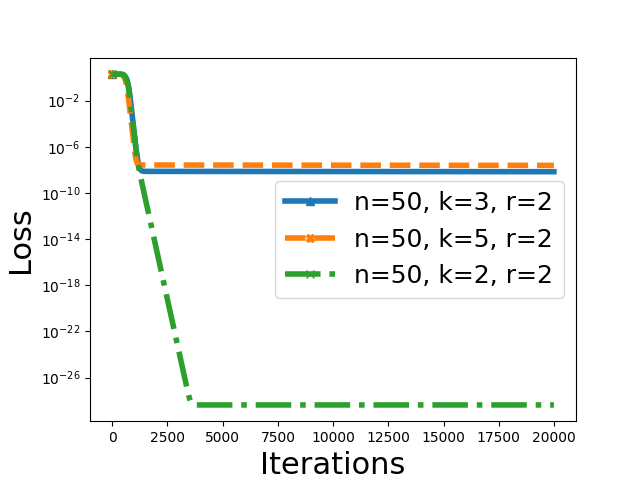
(a) Loss curve

(b) Curve of logarithm of loss: $\log_{T}\|X_{t}X_{t}^{\top}-M^{\star}\|_{F}^{2}$

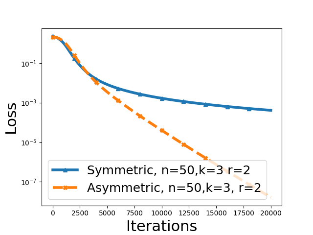
(c) Comparison between symmetric and asymmetric parameterization

Figure 1: Experiments on symmetric setting. $n$: ambient dimension. $k$: rank in our model. $r$: true rank. The first two figures show that the convergence rate of symmetric matrix factorization in the over-parameterized setting is about $\Theta(1/T^{2}),$ while the rate of the exact-parameterized setting is linear. 1(c) shows that using asymmetric parameterization is exponentially faster than symmetric parameterization. See §H for experimental details.

1.1 Setting 1: Symmetric Matrix Sensing with Symmetric Parameterization

We first consider the symmetric matrix sensing setting, where $M^{\star}\in\mathbb{R}^{n\times n}$ is a positive semi-definite matrix of rank $r\ll n$. A standard approach is to use a factored form $XX^{\top}$ to learn $M^{\star}$ where $X\in\mathbb{R}^{n\times k}$. We call this symmetric parameterization because $XX^{\top}$ is always symmetric and positive semi-definite. We will also introduce the asymmetric parameterization soon. We call the case when $k=r$ the exact-parameterization because the rank of $XX^{\top}$ matches that of $M^{\star}$. However, in practice, $r$ is often unknown, so one may choose some large enough $k>r$ to ensure the expressiveness of $XX^{\top}$, and we call this case over-parameterization.

We consider using gradient descent to minimize the standard $L_{2}$ loss for training: $L_{\mathrm{tr}}(X)=\frac{1}{2m}\sum_{i=1}^{m}\left(y_{i}-\langle A_{i},XX^{\top}\rangle\right)^{2}.$ We use the Frobneius norm of the reconstruction error as the performance metric:

$$L(X)=\frac{1}{2}\|XX^{\top}-M^{\star}\|^{2}_{F}.$$ (2)

We note that $L(X)$ is also the matrix factorization loss and can be viewed as a special case of $L_{\mathrm{tr}}$ when $\{A_{i}\}_{i=1}^{m}$ are random Gaussian matrices and the number of linear measurements goes to infinity.

For the exact-parameterization case, one can combine results in Stöger & Soltanolkotabi (2021) and Tu et al. (2016) to show that randomly initialized gradient descent enjoys an $\exp\left(-\Omega\left(T\right)\right)$ convergence rate where $T$ is the number of iterations. For the over-parameterization case, one can combine the results by Stöger & Soltanolkotabi (2021) and Zhuo et al. (2021) to show an $O\left(1/T^{2}\right)$ convergence rate upper bound, which is exponentially worse. This behavior has been empirically observed (Zhang et al., 2021b, 2023; Zhuo et al., 2021) without a rigorous proof. See Figure 1.

Contribution 1: $\Omega(1/T^{2})$ Lower Bound for Symmetric Over-Parameterization. Our first contribution is a rigorous exponential separation between the exact-parameterization and over-parameterization by proving an $\Omega(1/T^{2})$ convergence rate lower bound for the symmetric setting with the symmetric over-parameterization.

Theorem 1 (Informal).

Suppose we initialize $X$ with a Gaussian distribution with small enough variance that scales with $\alpha^{2}$, and use gradient descent with a small enough constant step size to optimize the matrix factorization loss (2). Let $X_{t}$ denote the factor matrix at the $t$-th iteration. Then, with high probability over the initialization, there exists $T^{(0)}>0$ such that we have

$$\|X_{t}X_{t}^{\top}-M^{\star}\|_{F}^{2}\geq\left(\frac{\alpha^{2}}{t}\right)^{2},\forall t\geq T^{(0)}.$$ (3)

Technical Insight:

We find the root cause of the slow convergence is from the redundant space in $XX^{\top}$, which converges to $0$ at a much slower rate compared to the signal space which converges to $M^{\star}$ with a linear rate. To derive the lower bound, we construct a potential function and use some novel analyses of the updating rule to show that the potential function decreases slowly after a few rounds. See the precise theorem and more technical discussions in Section 4.

1.2 Setting 2: Symmetric and Asymmetric Matrix Sensing with Asymmetric Parameterization

Next, we consider the more general asymmetric matrix sensing problem where the ground-truth $M^{\star}\in\mathbb{R}^{n_{1}\times n_{2}}$ is an asymmetric matrix of rank $r$. For this setting, we must use the asymmetric parameterization. Specifically, we use $FG^{\top}$ to learn $M^{\star}$ where $F\in\mathbb{R}^{n_{1}\times k}$ and $G\in\mathbb{R}^{n_{2}\times k}$. Same as in the symmetric case, exact-parameterization means $k=r$ and over-parameterization means $k>r$. We still use gradient descent to optimize the $L_{2}$ loss for training:

$$L_{\mathrm{tr}}(F,G) =\frac{1}{2m}\sum_{i=1}^{m}\left(y_{i}-\langle A_{i},FG^{\top}\rangle\right)^{2},$$ (4)

and the performance metric is still: $L(F,G)=\frac{1}{2}\|FG^{\top}-M^{\star}\|_{F}^{2}.$ To enable the analysis, we assume throughout the paper that the matrices $\{A_{i}\}_{i=1}^{m}$ satisfies the Restricted Isometry Property (RIP) of order $2k+1$ with parameter $\delta\leq\tilde{\mathcal{O}}(\frac{1}{\sqrt{kr}})$. (See Definition 5 for the detailed definition).

Also note that even for the symmetric matrix sensing problem where $M^{\star}$ is positive semi-definite, one can still use asymmetric parameterization. Although doing so seems unnecessary at the first glance, we will soon see using asymmetric parameterization enjoys an exponential gain.

Contribution 2: Global Exact Convergence of Gradient Descent for Asymmetric Exact-Parameterization with a Linear Convergence Rate

. Our second contribution is a global exact convergence result for randomly initialized gradient descent, and we show it enjoys a linear convergence rate.

Theorem 2 (Informal).

In the exact-parameterization setting ($k=r$), suppose we initialize $F$ and $G$ using a Gaussian distribution with small enough variance $\alpha^{2}$ and use gradient descent with a small enough constant step size to optimize the asymmetric matrix sensing loss (4). Let $F_{t}$ and $G_{t}$ denote the factor matrices at the $t$-the iteration. Then, with high probability over the random initialization, there exists $T^{(1)}>0$ such that we have

$$\|F_{t}G_{t}^{\top}-M^{\star}\|_{F}^{2}=\exp\left(-\Omega\left(t\right)\right),\forall t\geq T^{(1)}.$$ (5)

Compared to our results, prior results either require initialization to be close to optimal (Ma et al., 2021), or can only guarantee to find a point with an error of similar scale as the initialization (Soltanolkotabi et al., 2023). In contrast, our result only relies on random initialization and guarantees the error goes to $0$ as $t$ goes to infinity. Notably, this convergence rate is independent of $\alpha$. See Figure 2(a).

Naturally, such a result is expected by the works (Ma et al., 2021, Theorem 1) and (Soltanolkotabi et al., 2023). Indeed, one should be able to achieve the initial condition of (Ma et al., 2021, Theorem 1) by carefully inspecting the proof of (Soltanolkotabi et al., 2023) and additional work in translating different measures of balancing and closeness. Our proof is very different from (Ma et al., 2021) as we further decompose the factors $F$ and $G$, and we only need (Soltanolkotabi et al., 2023, Theroem 3.3) to deal with the initial phase.

Contribution 3: Global Exact Convergence of Gradient Descent for Asymmetric Over-Parameterization with an Initialization-Dependent Linear Convergence Rate.

Our next contribution is analogue theorem for the over-parameterization case with the caveat that the initialization scale $\alpha$ also appears in the convergence rate.

Theorem 3 (Informal).

In the over-parameterization setting ($k>r$), suppose we initialize $F$ and $G$ using a Gaussian distribution with small enough variance $\alpha^{2}$ and use gradient descent with a small enough constant step size to optimize the asymmetric matrix sensing loss (4). Let $F_{t}$ and $G_{t}$ denote the factor matrices at the $t$-the iteration. Then, with high probability over the random initialization, there exists $T^{(2)}>0$ such that we have

$$\|F_{t}G_{t}^{\top}-M^{\star}\|_{F}^{2}=\exp\left(-\Omega\left(\alpha^{2}t\right)\right),\forall t\geq T^{(2)}.$$ (6)

This is also the first global exact convergence result of randomly initialized gradient descent in the over-parameterized case. Recall that for the symmetric matrix sensing problem, even if $M^{\star}$ is positive semi-definite, one can still use an asymmetric parameterization $FG^{\top}$ to learn $M^{\star}$, and Theorem 3 still holds. Comparing Theorem 3 and Theorem 6, we obtain a surprising corollary:

For the symmetric matrix sensing problem, using asymmetric parameterization is exponentially faster than using symmetric parameterization.

Also notice that different from Theorem 2, the convergence rate of Theorem 3 also depends on the initialization scale $\alpha$ which we require it to be small. Empirically we verify this dependency is necessary. See Figure 2(b). We also study a special case in Section 5.1 to show the dependency on the initialization scale is necessary in the worst case.

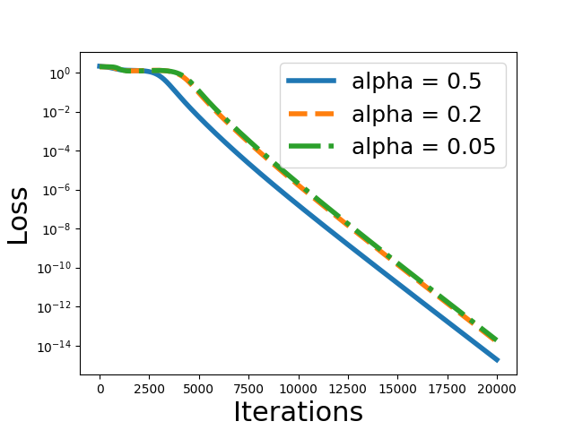
(a) Exact-parameterized case

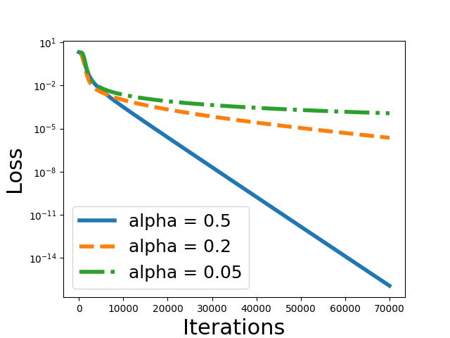
(b) Over-parameterized case

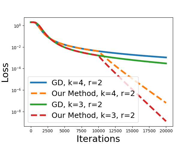
(c) Loss curve for our new method

Figure 2: Curve of asymmetric matrix sensing. Figure 2(a) shows that the convergence rate is linear and independent on the initialization scale under the exact-parameterized case. Figure 2(b) shows that the convergence rate is linear and dependent on the initialization scale under the over-parameterized case. When the initialization scale is larger, the convergence speed is faster. Figure 2(c) shows the efficacy of our new method. See §H for experimental details.

Technical Insight:

Our key technical finding that gives the exponential acceleration is the imbalance of $F$ and $G$. Denote the imbalance matrix $\Delta_{t}=F_{t}^{\top}F_{t}-G_{t}^{\top}G_{t}$. We show that the converge rate is linear when $\Delta_{t}$ is positive definite, and the rate depends on the minimum eigenvalue of $\Delta_{t}.$ We use imbalance initialization so that the minimum eigenvalue of $\Delta_{0}$ is proportional to $\alpha$, we can further show that the minimum eigenvalue $\Delta_{t}$ will not decrease too much, so the final convergence rate is linear. Furthermore, such a connection to $\alpha$ also inspires us to design a faster algorithm below.

Contribution 4: A Simple Algorithm with Initialization-Independent Linear Convergence Rate for Asymmetric Over-Parameterization.

Our key idea is to increase the degree of imbalance when $F$ and $G$ are close to the optimum. We develop a new simple algorithm to accelerate GD. The algorithm only involves transforming the factor matrices $F$ and $G$ in one of iteration to intensify the degree of imbalance (cf. Equation (26)).

Theorem 4 (Informal).

In the over-parameterization setting ($k>r$), suppose we initialize $F$ and $G$ using a Gaussian distribution with small enough variance $\alpha^{2}$, gradient descent with a small enough constant step size, and the procedure described in Section 6 to optimize the asymmetric matrix sensing loss (4). Let $F_{t}$ and $G_{t}$ denote the factor matrices at the $t$-the iteration. Then, with high probability over the random initialization, there exists $T^{(3)}>0$ such that we have

$$\|F_{t}G_{t}^{\top}-M^{\star}\|_{F}^{2}=\exp\left(-\Omega\left(t-T^{(3)}\right)\right),\forall t\geq T^{(3)}.$$ (7)

2 Related Work

The most relevant line of work studies the global convergence of randomly initialized gradient descent for matrix sensing with $L_{2}$ loss (Zhuo et al., 2021; Stöger & Soltanolkotabi, 2021; Soltanolkotabi et al., 2023; Tu et al., 2016). We compare our results with them in Table 1.

Table 1: Comparison of previous representative work. The second column shows that the results hold for symmetric matrix factorization/sensing or asymmetric matrix factorization/sensing. The third column lists different types of initialization, where “Random” means the algorithm uses random initialization (typically Gaussian), “Local” indicates a requirement for initialization to be close to the optimal point. The fourth column “exact-cnvrg” represents whether the loss will go to zero when round $T$ goes to infinity. The fifth column indicates whether the result applies to over-parameterization case or just the exact-parameterization case. The last column lists the convergence rate of algorithms with exact-convergence results.

	Is Symmetric	Init.	exact-cnvrg	$k$ Range	Rate
Stöger & Soltanolkotabi (2021)	Symmetric	Random	✗	$k\geq r$	N/A
Zhuo et al. (2021)	Symmetric	Local	✓	$k\geq r$	$\mathcal{O}(1/T^{2})$
Stöger & Soltanolkotabi (2021) + Zhuo et al. (2021)	Symmetric	Random	✓	$k\geq r$	$\mathcal{O}(1/T^{2})$
Soltanolkotabi et al. (2023)	Asymmetric	Random	✗	$k\geq r$	N/A
Tu et al. (2016)	Both	Local	✓	$k=r$	$\exp(-\Omega(T))$
Ma et al. (2021)	Asymmetric	Local	✓	$k=r$	$\exp(-\Omega(T))$
Theorem 9 (our paper)	Asymmetric	Random	✓	$k=r$	$\exp(-\Omega(T))$
Theorem 8 (our paper)	Asymmetric	Random	✓	$k>r$	$\exp(-\Omega(\alpha^{2}T))$
Theorem 6 (our paper)	Symmetric	Random	✓	$k\geq r$	$\Omega(1/T^{2})$

Matrix Sensing.

Matrix sensing aims to recover the low-rank matrix based on measurements. Candes & Recht (2012); Liu et al. (2012) propose convex optimization-based algorithms, which minimize the nuclear norm of a matrix, and Recht et al. (2010) show that projected subgradient methods can recover the nuclear norm minimizer. Wu & Rebeschini (2021) also propose a mirror descent algorithm, which guarantees to converge to a nuclear norm minimizer. See (Davenport & Romberg, 2016) for a comprehensive review.

Non-Convex Low-Rank Factorization Approach.

The nuclear norm minimization approach involves optimizing over a $n\times n$ matrix, which can be computationally prohibitive when $n$ is large. The factorization approach tries to use the product of two matrices to recover the underlying matrix, but this formulation makes the optimization problem non-convex and is significantly more challenging for analysis. For the exact-parameterization setting ($k=r$), Tu et al. (2016); Zheng & Lafferty (2015) shows the linear convergence of gradient descent when starting at a local point that is close to the optimal point. This initialization can be implemented by the spectral method. For the over-parameterization scenario ($k>r$), in the symmetric setting, Stöger & Soltanolkotabi (2021) shows that with a small initialization, the gradient descent achieves a small error that dependents on the initialization scale, rather than the exact-convergence. Zhuo et al. (2021) shows exact convergence with $\mathcal{O}(1/T^{2})$ convergence rate in the overparamterization setting. These two results together imply the global convergence of randomly initialized GD with an $O\left(1/T^{2}\right)$ convergence rate upper bound. Jin et al. (2023) also provides a fine-grained analysis of the GD dynamics. More recently, Zhang et al. (2021b, 2023) empirically observe that in practice, in the over-parameterization case, GD converges with a sublinear rate, which is exponentially slower than the rate in the exact-parameterization case, and coincides with the prior theory’s upper bound (Zhuo et al., 2021). However, no rigorous proof of the lower bound is given whereas we bridge this gap. On the other hand, Zhang et al. (2021b, 2023) propose a preconditioned GD algorithm with a shrinking damping factor to recover the linear convergence rate. Xu et al. (2023) show that the preconditioned GD algorithm with a constant damping factor coupled with small random initialization requires a less stringent assumption on $\mathcal{A}$ and achieves a linear convergence rate up to some prespecified error. Ma & Fattahi (2023) study the performance of the subgradient method with $L_{1}$ loss under a different set of assumptions on $\mathcal{A}$ and showed a linear convergence rate up to some error related to the initialization scale. We show that by simply using the asymmetric parameterization, without changing the GD algorithm, we can still attain the linear rate.

For the asymmetric matrix setting, many previous works (Ye & Du, 2021; Ma et al., 2021; Tong et al., 2021; Ge et al., 2017; Du et al., 2018a; Tu et al., 2016; Zhang et al., 2018a, b; Wang et al., 2017; Zhao et al., 2015) consider the exact-parameterization case ($k=r$). Tu et al. (2016) adds a balancing regularization term $\frac{1}{8}\|F^{\top}F-G^{\top}G\|_{F}^{2}$ to the loss function, to make sure that $F$ and $G$ are balanced during the optimization procedure and obtain a local convergence result. More recently, some works (Du et al., 2018a; Ma et al., 2021; Ye & Du, 2021) show GD enjoys an auto-balancing property where $F$ and $G$ are approximately balanced; therefore, additional balancing regularization is unnecessary. In the asymmetric matrix factorization setting, Du et al. (2018a) proves a global convergence result of GD with a diminishing step size and the GD recovers $M^{\star}$ up to some error. Later, Ye & Du (2021) gives the first global convergence result of GD with a constant step size. Ma et al. (2021) shows linear convergence of GD with a local initialization and a larger stepsize in the asymmetric matrix sensing setting. Although exact-parameterized asymmetric matrix factorization and matrix sensing problems have been explored intensively in the last decade, our understanding of the over-parameterization setting, i.e., $k>r$, remains limited. Jiang et al. (2022) considers the asymmetric matrix factorization setting, and proves that starting with a small initialization, the vanilla gradient descent sequentially recovers the principled component of the ground-truth matrix. Soltanolkotabi et al. (2023) proves the convergence of gradient descent in the asymmetric matrix sensing setting. Unfortunately, both works only prove that GD achieves a small error when stopped early, and the error depends on the initialization scale. Whether the gradient descent can achieve exact-convergence remains open, and we resolve this problem by novel analyses. Furthermore, our analyses highlight the importance of the imbalance between $F$ and $G$.

Lastly, we want to remark that we focus on gradient descent for $L_{2}$ loss, there are works on more advanced algorithms and more general losses (Tong et al., 2021; Zhang et al., 2021b, 2023, 2018a, 2018b; Ma & Fattahi, 2021; Wang et al., 2017; Zhao et al., 2015; Bhojanapalli et al., 2016; Xu et al., 2023). We believe our theoretical insights are also applicable to those setups.

Landscape Analysis of Non-convex Low-rank Problems.

The aforementioned works mainly focus on studying the dynamics of GD. There is also a complementary line of works that studies the landscape of the loss functions, and shows the loss functions enjoy benign landscape properties such as (1) all local minima are global, and (2) all saddle points are strict Ge et al. (2017); Zhu et al. (2018); Li et al. (2019); Zhu et al. (2021); Zhang et al. (2023). Then, one can invoke a generic result on perturbed gradient descent, which injects noise to GD Jin et al. (2017), to obtain a convergence result. There are some works establishing the general landscape analysis for the non-convex low-rank problems. We remark that injecting noise is required if one solely uses the landscape analysis alone because there exist exponential lower bounds for standard GD (Du et al., 2017).

Slowdown Due to Over-parameterization.

Similar exponential slowdown phenomena caused by over-parameterization have been observed in other problems beyond matrix recovery, such as teacher-student neural network training (Xu & Du, 2023; Richert et al., 2022) and Expectation-Maximization algorithm on Gaussian mixture model (Wu & Zhou, 2021; Dwivedi et al., 2020).

3 Preliminaries

Norm and Big-$\mathcal{O}$ Notations.

Given a vector $v$, we use $\|v\|$ to denote its Euclidean norm. For a matrix $M$, we use $\|M\|$ to denote its spectral norm and $\|M\|_{F}$ Frobenius norm. The notations $\mathcal{O}(\cdot),\Theta(\cdot),$ and $\Omega(\cdot)$ in the rest of the paper only omit absolute constants.

Asymmetric Matrix Sensing.

Our primary goal is to recover an unknown fixed rank $r$ matrix $M^{\star}\in\mathbb{R}^{n_{1}\times n_{2}}$ from data $(y_{i},A_{i})$, $i=1,\dots,m$ satisfying $y_{i}=\langle A_{i},M^{\star}\rangle=\mathrm{tr}(A_{i}^{\top}M^{\star}),i=1,\dots,m,\quad\text{or compactly}\quad y=\mathcal{A}(M^{\star}),$ where $y\in\mathbb{R}^{m}$ and $\mathcal{A}:\mathbb{R}^{n_{1}\times n_{2}}\rightarrow\mathbb{R}^{m}$ is a linear map with $[\mathcal{A}(M)]_{i}=\mathrm{tr}(A_{i}^{\top}M)$. We further denote the singular values of $M^{\star}$ as $\sigma_{1}\geq\dots\geq\sigma_{r}>\sigma_{r+1}=0=\cdots=\sigma_{n}$, the condition number $\kappa=\frac{\sigma_{1}}{\sigma_{r}}$, and the diagonal singular value matrix as $\Sigma$ with $(\Sigma)_{ii}=\sigma_{i}$. To recover $M^{\star}$, we minimize the following loss function:

$$L_{\mathrm{tr}}(F,G)=\frac{1}{2}\|\mathcal{A}(FG^{\top})-y\|^{2},$$ (8)

where $F,G\in\mathbb{R}^{n\times k}$, where $k\geq r$ is the user-specified rank. The gradient descent update rule with a step size $\eta>0$ with respect to loss (8) can be written explicitly as

$$F_{t+1}=F_{t}-\eta\mathcal{A}^{*}\mathcal{A}(F_{t}G_{t}^{\top}-\Sigma)G_{t},~{}~{}~{}G_{t+1}=G_{t}-\eta(\mathcal{A}^{*}\mathcal{A}(F_{t}G_{t}^{\top}-\Sigma))^{\top}F_{t},$$ (9)

where $\mathcal{A}^{*}:\mathbb{R}^{m}\rightarrow\mathbb{R}^{n\times n}$ is the adjoint map of $\mathcal{A}$ and admits an explicit form: $\mathcal{A}^{*}(z)=\sum_{i=1}^{m}z_{i}A_{i}$.

To make the problem approachable, we shall make the following standard assumption on $\mathcal{A}$: Restricted Isometry Property (RIP) (Recht et al., 2010).

Definition 5 (Restricted Isometry Property).

An operator $\mathcal{A}:\mathbb{R}^{n_{1}\times n_{2}}\to\mathbb{R}^{m}$ satisfies the Restricted Isometry Property of order $r$ with constant $\delta>0$ if for all matrices $M:\mathbb{R}^{n_{1}\times n_{2}}$ with rank at most $r$, we have $(1-\delta)\|M\|^{2}_{F}\leq\|\mathcal{A}(M)\|^{2}\leq(1+\delta)\|M\|^{2}_{F}.$

From (Candes & Plan, 2011), if the matrix $A_{i}$ has i.i.d. $N(0,\frac{1}{m})$, the operator $\mathcal{A}$ has RIP of order $2k+1$ with constant $\delta\in(0,1)$ when $m=\widetilde{\Omega}\left(\frac{nk}{\delta^{2}}\right)$. Thus, $m=\widetilde{\Omega}(nk^{2}r)$ is needed with 21.

Diagonal Matrix Simplification.

Since both the RIP and the loss are invariant to orthogonal transformation, we assume without loss generality that $M^{\star}=\Sigma$ in the rest of the paper for clarity, following prior work (Ye & Du, 2021; Jiang et al., 2022). For the same reason, we also assume $n_{1}=n_{2}=n$ to simplify notations, and our results can be easily extended to $n_{1}\neq n_{2}$.

Symmetric Matrix Factorization.

In this setting, we further assume $M^{\star}$ is symmetric and positive semidefinite, and $\mathcal{A}$ is the identity map. Since $M^{\star}$ admits a factorization $M^{\star}=F_{\star}F_{\star}^{\top}$ for some $F_{\star}\in\mathbb{R}^{n\times r}$, we can force the factor $F=G=X$ in (8) and the loss becomes $L(X)=\frac{1}{2}\|XX^{\top}-\Sigma\|_{F}^{2}.$ Here, the factor $X\in\mathbb{R}^{n\times k}$. We shall focus on the over-parameterization setting, i.e., $k>r$ in the Setion 4 below. The gradient descent with a step size $\eta>0$ becomes

$$X_{t+1}=X_{t}-2\eta(X_{t}X_{t}^{\top}-\Sigma)X_{t}.$$ (10)

4 Lower Bound of Symmetric Matrix Factorization

We present a sublinear lower bound of the convergence rate of the gradient descent (10) for symmetric matrix factorization starting from a small random initialization. Our result supports the empirical observations that overparmetrization slows down gradient descent (Zhuo et al., 2021; Zhang et al., 2021b, 2023) and Figure 1.

Theorem 6.

Let $X_{0}=\alpha\cdot\tilde{X_{0}}$, where each entry is independent initialized from Gaussian distribution $\mathcal{N}(0,1/k)$. For some universal constants $c_{i},1\leq i\leq 7$, if the gradient descent method (10) starting at $X_{0}$ with the initial scale $\alpha$, the search rank $k$, and the stepsize $\eta$ satisfying that

$$0<\alpha\leq\frac{c_{1}\sqrt{\sigma_{1}}}{\sqrt{n}\log(r\sqrt{n})},\quad k\geq c_{2}\left((r\kappa)^{2}\log(r\sqrt{\sigma_{1}}/\alpha)\right)^{4},\quad\text{and}\quad 0<\eta\leq\frac{c_{3}}{n^{2}\kappa\sigma_{1}},$$ (11)

then with probability at least $1-2n^{2}\exp(-\sqrt{c_{4}k})-2n\exp(-c_{5}k/4)$, for all $t\geq T^{(0)}=\frac{c_{6}\log(r\sqrt{\sigma_{1}})/\alpha}{\eta\sigma_{r}}$, we have

$$\|X_{t}X_{t}^{\top}-\Sigma\|_{F}^{2}\geq\left(\frac{c_{7}\log(\sqrt{r\sigma_{1}}/\alpha)\alpha^{2}}{8\sigma_{r}\eta nt}\right)^{2},\quad\forall t\geq T^{(0)}.$$ (12)

The proof of Theorem 1 demonstrates that, following a rapid convergence phase, the gradient descent eventually transitions to a sublinear convergence rate. Also, the over-parameterization rank $k$ is subject to a lower bound requirement in Eq. (11) that depends on $\alpha$. However, since $\alpha$ only appears in the logarithmic term, this requirement is not overly restrictive. It is also consistent with the phenomenon that the gradient descent first converges to a small error that depends on $\alpha$ with a linear convergence rate (Stöger & Soltanolkotabi, 2021), since our lower bound has a term $\alpha^{4}$.

4.1 Proof Sketch of Theorem 6

We provide a proof sketch of Theorem 6 in this section, deferring the details to Appendix B.

The main intuition of Theorem 6 is that the last $n-r$ rows of $X_{t}$, corresponding to the space of $0$ eigenvalues of $\Sigma$, converge to $0$ at speed no faster than $\frac{1}{T^{2}}$. To make this intuition precise, for each $t\geq 0$, we let $X_{t}\in\mathbb{R}^{n\times k}=[x_{1}^{t},\cdots,x_{n}^{t}]^{\top}$ where $x_{i}^{t}\in\mathbb{R}^{k}$. We let the potential function be $A_{t}=\sum_{i>r}\|x_{i}^{t}\|^{2}$. We aim to show the following two key inequalities,

$$\|x_{i}^{T}\|^{2}\geq\alpha^{2}/8,\text{ for all $i>r$},$$ (13a)

$$A_{t+1}\geq A_{t}(1-\mathcal{O}(\eta A_{t})),\text{ for all $t\geq T^{(0)}$}.$$ (13b)

Suppose (13) is true, then it implies that $A_{t}\geq\mathcal{O}\left(\frac{\alpha^{2}}{t}\right)$ for all $t\geq T^{(0)}$. Since $(X_{t}X_{t}^{\top}-\Sigma)_{ii}=\|x_{i}\|^{2}$, the lower bound (12) is established by noting that $\|X_{t}X_{t}^{\top}-\Sigma\|_{F}^{2}\geq\sum_{i>r}\|x_{i}^{t}\|^{4}\geq A_{t}^{2}/n$, where the last inequality uses the Cauchy’s inequality. See more details in Appendix B.

5 Convergence of Asymmetric Matrix Sensing

Here, we investigate the dynamic of GD in the context of the asymmetric matrix sensing problem. Surprisingly, we demonstrate that the convergence rate of gradient descent for asymmetric matrix sensing problems is linear, so long as the initialization is imbalanced. However, this linear rate is contingent upon the chosen initialization scale.

5.1 A Toy Example of Asymmetric Matrix Factorization

We first use a toy example of asymmetric matrix factorization to demonstrate the behavior of GD. If we assume $\mathcal{A}$ is the identity map, and the loss and the GD update become

$$L(F,G)= \frac{1}{2}\|FG^{\top}-\Sigma\|_{F}^{2}.$$ (14)

$$F_{t+1}=F_{t}-\eta(F_{t}G_{t}^{\top}-\Sigma)G_{t},~{}~{}~{} G_{t+1}=G_{t}-\eta(F_{t}G_{t}^{\top}-\Sigma)^{\top}F_{t}$$ (15)

The following theorem tightly characterizes the convergence rate for a toy example.

Theorem 7.

Consider the asymmetric matrix factorization (14), with $k=r+1$. Choose $\eta\in[0,1/6]$ and $\alpha\in[0,1]$. Assume that the diagonal matrix $\Sigma=\text{diag}(\sigma_{1},\dots,\sigma_{n})$, where $\sigma_{i}=1$ for $i\leq r$ and is $0$ otherwise. Also assume that gradient descent (15) starts at $F_{0},G_{0}$, where $(F_{0})_{ii}=\alpha$ for $1\leq i\leq k$, and $(G_{0})_{ii}=\alpha$ for $1\leq i\leq r$, $(G_{0})_{ii}=\alpha/3$ for $i=r+1,$ and all other entries of $F_{0}$ and $G_{0}$ are zero. Then, the iterate $(F_{t},G_{t})$ of (15) satisfies that

$$\frac{\alpha^{4}}{36}(1-4\eta\alpha^{2})^{2t}\leq\|F_{t}G_{t}^{\top}-\Sigma\|_{F}^{2}\leq 4n\cdot(1-\eta\alpha^{2}/4)^{(t-T_{1})},\;\forall t\geq T_{1}.$$

where $T_{1}=c_{1}\log(1/\alpha)/\eta$, and $c_{1}$ is a universal constant.

The above initialization implicitly assumes that we know the singular vectors of $\Sigma$. Such an assumption greatly simplifies our presentations below. Note that we have a different initialization scale for $F_{t}$ and $G_{t}$. As we shall see, such an imbalance is the key to establishing the convergence of $F_{t}G_{t}^{\top}$.

We introduce some notations before our proof. Denote the matrix of the first $r$ row of $F,G$ as $U,V\in\mathbb{R}^{r\times k}$ respectively, and the matrix of the last $n-r$ row of $F,G$ as $J,K\in\mathbb{R}^{(n-r)\times k}$ respectively. Further denote the corresponding iterate of gradient descent as $U_{t}$, $V_{t}$, $J_{t}$, and $K_{t}$. The difference $F_{t}G_{t}^{\top}-\Sigma$ can be written in a block form as $F_{t}G_{t}^{\top}-\Sigma=\begin{pmatrix}U_{t}V_{t}^{\top}-\Sigma_{r}&J_{t}V_{t}^{\top}\\ U_{t}K_{t}^{\top}&J_{t}K_{t}^{\top}\\ \end{pmatrix}$ where $\Sigma_{r}\in\mathbb{R}^{r\times r}$ is the identity matrix. Hence, we may bound $\|F_{t}G_{t}^{\top}-\Sigma\|$ by

$$\|J_{t}K_{t}^{\top}\|\leq\|F_{t}G_{t}^{\top}-\Sigma\|\leq\|U_{t}V_{t}^{\top}-\Sigma_{r}\|+\|J_{t}V_{t}^{\top}\|+\|U_{t}K_{t}^{\top}\|+\|J_{t}K_{t}^{\top}\|.$$ (16)

From (16), we shall upper bound $\|U_{t}V_{t}^{\top}-\Sigma_{r}\|$, $\|J_{t}V_{t}^{\top}\|$, $\|U_{t}K_{t}^{\top}\|$, and $\|J_{t}K_{t}^{\top}\|$, and lower bound $\|J_{t}K_{t}\|^{\top}$. Let us now prove Theorem 7.

Proof.

With our particular initialization and the formula of gradient descent (15), we have the following equality for all $t$:

$$U_{t}K_{t}^{\top}=0,\quad J_{t}V_{t}^{\top}=0,\quad U_{t}=V_{t},\quad J_{t}=a_{t}A,\quad K_{t}=b_{t}A,\quad U_{t}=(\alpha_{t}I_{r},0),$$ (17a)

$$a_{0}=\alpha,\quad b_{0}=\alpha/3,\quad\alpha_{0}=\alpha$$ (17b)

$$a_{t+1}=a_{t}-\eta a_{t}b_{t}^{2},$$ (17c)

$$b_{t+1}=b_{t}-\eta a_{t}^{2}b_{t}.$$ (17d)

$$\alpha_{t+1}=\alpha_{t}(1+\eta-\eta\alpha_{t}^{2}),$$ (17e)

where $A\in\mathbb{R}^{(n-r)\times k}$ is the matrix that $(A)_{1k}=1$ and other elements are all zero, and $a_{t},b_{t},\alpha_{t}\in\mathbb{R}$. We leave the detailed verification of (17) to Appendix C. By considering (16) and (17), we see that we only need to keep track of three sequences $a_{t},b_{t}$, $\alpha_{t}$. In particular, we have the following inequalities for $a_{t},b_{t},\alpha_{t}$ for all $t\geq T_{1}$:

$$a_{t}\in\left[\frac{1}{2}\alpha,\alpha\right],\;b_{t}\in\left[\frac{\alpha}{3}(1-4\eta\alpha^{2})^{t},\;\frac{\alpha}{3}(1-\frac{\eta\alpha^{2}}{4})^{t/2}\right],\;\text{and}\;|\alpha_{t}-1|\leq(1-\eta/2)^{t-T_{1}}.$$ (18)

It is then easy to derive the upper and lower bounds. We leave the detail in checking (18) to Appendix C. Our proof is complete. ∎

Technical Insight.

This proof of the toy case tells us why the imbalance initialization in the asymmetric matrix factorization helps us to break the $\Omega(1/T^{2})$ convergence rate lower bound of the symmetric case. Since we initialize $F_{0}$ and $G_{0}$ with a different scale, this difference makes the norm of $K$ converge to zero at a linear rate while keeping $J$ larger than a constant. However, in the symmetric case, we have $a_{t}=b_{t}$, so they must both converge to zero when the loss goes to zero (as $\|F_{t}G_{t}^{\top}-\Sigma\|\geq a_{t}b_{t}$), leading to a sublinear convergence rate. In short, the imbalance property in the initialization causes faster convergence in the asymmetric case.

5.2 Theoretical Results for Asymmetric Matrix Sensing

Motivated by the toy case in Section 5.1, the imbalance property is the key ingredient for a linear convergence rate. If we use a slightly imbalanced initialization $F_{0}=\alpha\cdot\tilde{F}_{0},G_{0}=(\alpha/3)\cdot\tilde{G}_{0}$, where the elements of $\tilde{F}_{0}$ and $\tilde{G}_{0}$ are $\mathcal{N}(0,1/n)$, we have $\|F_{0}^{\top}F_{0}-G_{0}^{\top}G_{0}\|=\Omega(\alpha^{2})$. Then, we can show that the imbalance property keeps true when the step size is small, and thus, the gradient descent (9) converges with a linear rate similar to the toy case.

Our result is built upon the recent work (Soltanolkotabi et al., 2023) in dealing with the initial phase. Define the following quantities $\alpha_{0},\eta_{0}$ according to (Soltanolkotabi et al., 2023, Theorem 1):

$$\alpha_{0}=\frac{c\sqrt{\sigma_{1}}}{k^{5}\max\{2n,k\}^{2}}\cdot\left(\frac{\sqrt{k}-\sqrt{r-1}}{\kappa^{2}\sqrt{\max\{2n,k\}}}\right)^{C\kappa},\eta_{0}=\frac{c}{k^{5}\sigma_{1}\log\left(\frac{2\sqrt{2\sigma_{1}}}{\alpha(\sqrt{k}-\sqrt{r-1}}\right)},$$ (19)

where $c$ and $C$ are some numerical constants. Below, we show exact convergence results for both $k=r$ and $k>r$.

Theorem 8.

Consider the matrix sensing problem (4) and the gradient descent (9). For some numerical constants $c_{i}>0$, $1\leq i\leq 7$, if the search rank $k$ satisfies $r<k<\frac{n}{8}$, the initial scale $\alpha$ and $\eta$ satisfy

$$\alpha\leq\min\left\{c_{1}\kappa^{-2}\sqrt{\sigma_{r}},\alpha_{0}\right\},\ \ \ \ \ \eta\leq\min\Big{\{}c_{1}\alpha^{4}/\sigma_{1}^{3},\eta_{0}\Big{\}},$$ (20)

where $\alpha_{0},\eta_{0}$ are defined in (19), and the operator $\mathcal{A}$ has the RIP of order $2k+1$ with constant $\delta$ satisfying

$$\delta\sqrt{2k+1}\leq\min\left\{c_{1}\kappa^{-6}\log^{-1}(\sqrt{\sigma_{r}}/(n\alpha)),\frac{c_{1}}{\kappa^{3}\sqrt{r}},1/128\right\},$$ (21)

then the gradient descent (9) starting with $F_{0}=\alpha\cdot\tilde{F}_{0},G_{0}=(\alpha/3)\cdot\tilde{G}_{0}$, where $\tilde{F}_{0},\tilde{G}_{0}\in\mathbb{R}^{n\times k}$ whose entries are i.i.d. $\mathcal{N}(0,1/n)$, satisfies that

$$\|F_{t}G_{t}^{\top}-\Sigma\|_{F}^{2}\leq\frac{\sigma_{r}^{4}n}{c_{7}\alpha^{4}\kappa^{2}}\left(1-\frac{\eta\alpha^{2}}{8}\right)^{t/4},\quad\forall t\geq T^{(1)},$$ (22)

with probability at least $1-2e^{-c_{2}n}-c_{3}e^{-c_{4}k}-(c_{5}\upsilon)^{(k-r+1)}$, where $T^{(1)}=c_{6}\log(\sqrt{\sigma_{r}}/n\alpha\upsilon)/\eta\sigma_{r})$ and $v\in[0,1]$ is an arbitrary parameter.

Next, we state our results on exact parametrization.

Theorem 9.

Consider the same setting as Theorem 8 except assuming $k=r$, then with probability at least $1-2e^{-c_{2}n}-c_{3}e^{-c_{4}k}-c_{5}\upsilon,$ the gradient descent (9) achieves

$$\|F_{t}G_{t}^{\top}-\Sigma\|_{F}^{2}\leq 2n\sigma_{r}\cdot\left(1-\frac{\eta\sigma_{r}^{2}}{64\sigma_{1}}\right)^{t},\quad\forall t\geq T^{(2)},$$ (23)

where $T^{(2)}=c_{7}\log(\sqrt{\sigma_{r}}/n\alpha\upsilon)/\eta\sigma_{r})$ for some numerical constant $c_{7}$.

Now we highlight two bullet points of Theorem 8 and 9.

Exact Convergence.

The main difference between the above theorems and previous convergence results in (Soltanolkotabi et al., 2023) is that we prove the exact convergence property, i.e., the loss finally degenerates to zero when $T$ tends to infinity (cf. Table 1). Moreover, we prove that the convergence rate of the gradient descent depends on the initialization scale $\alpha$, which matches our empirical observations in Figure 2.

Discussions about Parameters.

First, since we utilize the initial phase result in (Soltanolkotabi et al., 2023) to guarantee that the loss degenerates to a small scale, our parameters $\delta$, $\alpha$, and $\eta$ should satisfy the requirement $\delta_{0}=\mathcal{O}(\frac{1}{\kappa^{3}\sqrt{r}}),\alpha_{0},\eta_{0}$ in (Soltanolkotabi et al., 2023). We further require $\delta_{2k+1}=\widetilde{\mathcal{O}}(\kappa^{-6})$, $\alpha=\mathcal{O}(\kappa^{-2}\sqrt{\sigma_{r}})$, which are both polynomials of the conditional number $\kappa.$ In addition, the step size $\eta$ has the requirement $\eta=\mathcal{O}(\alpha^{4}/\sigma_{1}^{3})$, which can be much smaller than the requirements $\eta=\widetilde{\mathcal{O}}(1/\kappa^{5}\sigma_{1})$ in (Soltanolkotabi et al., 2023). In Section 6, we propose a novel algorithm that allows larger learning rate which is independent of $\alpha.$

Technical insight.

Similar to the asymmetric matrix factorization case in the proof of Theorem 7, the main effort is in characterizing the behavior of $J_{t}K_{t}^{\top}$. In particular, the update rule of $K_{t}$ is

$$K_{t+1}=K_{t}(1-\eta F_{t}^{\top}F_{t})+\eta E,$$ (24)

where $E$ is some error matrix since $\mathcal{A}$ is not an identity. Because of our initialization, we know the following holds for $t=0$ and $\Delta_{t}=F^{\top}_{t}F_{t}-G^{\top}_{t}G_{t}$,

$$c\alpha^{2}I\preceq\Delta_{t}\preceq C\alpha^{2}I.$$ (25)

for some numerical constant $c,C>0$. Hence, we can show $\|K_{t}\|$ shrinks towards $0$ so long as (24) is true, $E=0$, and $G_{t}$ is well-bounded. Indeed, we can prove (25) and $G_{t},J_{t}$ upper bounded for all $t\geq 0$ via a proper induction. We may then be tempted to conclude $J_{t}K_{t}^{\top}$ converges to $0$. However, the actual analysis of the gradient descent (9) for matrix sensing is much more complicated due to the error $E$. It is now unclear whether $\|K_{t}\|$ will shrink under (25). To deal with it, we further consider the structure of $E$. We leave the details to Appendix D.

6 A Simple and Fast Convergence Method

As discussed in Section 5, the fundamental reason that the convergence rate depends on the initialization scaling $\alpha$ is that the imlabace between $F$ and $G$ determines the convergence rate, but the imbalance between $F$ and $G$ remains at the initialization scale. This observation motivates us to do a straightforward additional step in one iteration to intensify the imbalance. Specifically, suppose at the $T_{0}$ iteration we have reached a neighborhood of an optimum that satisfies: $\|\mathcal{A}^{*}\mathcal{A}(\widetilde{F}_{T^{(3)}}\widetilde{G}_{T^{(3)}}^{\top}-\Sigma)\|\leq\gamma$ where the radius $\sigma_{r}^{1/4}\cdot\|F_{T^{(3)}}G_{T^{(3)}}^{\top}\|^{3/4}/8$ is chosen for some technical reasons (cf. Section F). Here, we use $\widetilde{F}_{t}$ and $\widetilde{G}_{t}$ to denote the iterates before we make the change we describe below and $F_{t}$ and $G_{t}$ to denote the iterates after make the change.

Let the singular value decomposition of $\widetilde{F}_{T^{(3)}}=A\Sigma^{\prime}B$ with the diagonal matrix $\Sigma^{\prime}\in\mathbb{R}^{k\times k}$ and $\Sigma^{\prime}_{ii}=\sigma^{\prime}_{i}$, then let $\Sigma_{inv}\in\mathbb{R}^{k\times k}$ be a diagonal matrix and $(\Sigma_{inv})_{ii}=\beta/\sigma^{\prime}_{i}$ for some small constant $\beta=O(\sigma_{r})$, then we transform the matrix $F_{T^{(3)}},G_{T^{(3)}}$ by

$$F_{T^{(3)}}=\widetilde{F}_{T^{(3)}}B^{\top}\Sigma_{inv},G_{T^{(3)}}=\widetilde{G}_{T^{(3)}}B\Sigma_{inv}^{-1}$$ (26)

We can show that, when $F$ and $G$ have reached a local region of an optimum, their magnitude will have similar scale as $M^{\star}$. Therefore, the step Equation (26) can create an imbalance between $F$ and $G$ as large the magnitude of $M^{\star}$, which is significantly larger than the initial scaling $\alpha$. The following theorem shows we can obtain a convergence rate independent of the initialization scaling $\alpha$. The proof is deferred to Appendix F.

Theorem 10.

With the same setting as Theorem 8, suppose that at the step $T^{(3)}$ we have $\|\mathcal{A}^{*}\mathcal{A}(\widetilde{F}_{T^{(3)}}\widetilde{G}_{T^{(3)}}^{\top}-\Sigma)\|\leq\gamma$ for some $\gamma>0$, and we do one step as in Equation (26). Then, with probability at least $1-2e^{-c_{2}n}-c_{3}e^{-c_{4}k}-(c_{5}\upsilon)^{(k-r+1)}$, we have for all $t>T^{(3)}$,

$$\|F_{t}G_{t}^{\top}-\Sigma\|_{F}^{2}\leq\frac{n\beta^{12}}{\sigma_{1}^{4}}\left(1-\frac{\eta\beta^{2}}{2}\right)^{2(t-T^{(3)})},$$

so long as $0<c_{7}\gamma^{1/6}\sigma_{1}^{1/3}\leq\beta\leq c_{8}\sigma_{r}$, and the step size satisfies $\eta\leq c_{9}\beta^{2}/\sigma_{1}^{2}$ from the iteration $T^{(3)}\leq c_{10}\log(\sqrt{\sigma_{r}}/n\alpha\upsilon)/\eta\sigma_{r}$ for some positive numerical constants $c_{i},i=1,\dots,10$.

7 Conclusion

This paper demonstrated qualitatively different behaviors of GD in the exact-parameterization and over-parameterization scenarios in symmetric and asymmetric settings. For the symmetric matrix sensing problem, we provide a $\Omega(1/T^{2})$ lower bound. For the asymmetric matrix sensing problem, we show that the gradient descent converges at a linear rate, where the rate is dependent on the initialization scale. Moreover, we introduce a simple procedure to get rid of the initialization scale dependency. We believe our analyses are also useful for other problems, such as deep linear networks.

Appendix

Appendix

Appendix A Related Work

Matrix Sensing.

Matrix sensing aims to recover the low-rank matrix based on measurements. Candes & Recht (2012); Liu et al. (2012) propose convex optimization-based algorithms, which minimize the nuclear norm of a matrix, and Recht et al. (2010) show that projected subgradient methods can recover the nuclear norm minimizer. Wu & Rebeschini (2021) also propose a mirror descent algorithm, which guarantees to converge to a nuclear norm minimizer. See (Davenport & Romberg, 2016) for a comprehensive review.

Non-Convex Low-Rank Factorization Approach.

The nuclear norm minimization approach involves optimizing over a $n\times n$ matrix, which can be computationally prohibitive when $n$ is large. The factorization approach tries to use the product of two matrices to recover the underlying matrix, but this formulation makes the optimization problem non-convex and is significantly more challenging for analysis. For the exact-parameterization setting ($k=r$), Tu et al. (2016); Zheng & Lafferty (2015) shows the linear convergence of gradient descent when starting at a local point that is close to the optimal point. This initialization can be implemented by the spectral method. For the over-parameterization scenario ($k>r$), in the symmetric setting, Stöger & Soltanolkotabi (2021) shows that with a small initialization, the gradient descent achieves a small error that dependents on the initialization scale, rather than the exact-convergence. Zhuo et al. (2021) shows exact convergence with $\mathcal{O}(1/T^{2})$ convergence rate in the overparamterization setting. These two results together imply the global convergence of randomly initialized GD with an $O\left(1/T^{2}\right)$ convergence rate upper bound. Jin et al. (2023) also provides a fine-grained analysis of the GD dynamics. More recently, Zhang et al. (2021b, 2023) empirically observe that in practice, in the over-parameterization case, GD converges with a sublinear rate, which is exponentially slower than the rate in the exact-parameterization case, and coincides with the prior theory’s upper bound (Zhuo et al., 2021). However, no rigorous proof of the lower bound is given whereas we bridge this gap. On the other hand, Zhang et al. (2021b, 2023) propose a preconditioned GD algorithm with a shrinking damping factor to recover the linear convergence rate. Xu et al. (2023) show that the preconditioned GD algorithm with a constant damping factor coupled with small random initialization requires a less stringent assumption on $\mathcal{A}$ and achieves a linear convergence rate up to some prespecified error. Ma & Fattahi (2023) study the performance of the subgradient method with $L_{1}$ loss under a different set of assumptions on $\mathcal{A}$ and showed a linear convergence rate up to some error related to the initialization scale. We show that by simply using the asymmetric parameterization, without changing the GD algorithm, we can still attain the linear rate.

For the asymmetric matrix setting, many previous works (Ye & Du, 2021; Ma et al., 2021; Tong et al., 2021; Ge et al., 2017; Du et al., 2018a; Tu et al., 2016; Zhang et al., 2018a, b; Wang et al., 2017; Zhao et al., 2015) consider the exact-parameterization case ($k=r$). Tu et al. (2016) adds a balancing regularization term $\frac{1}{8}\|F^{\top}F-G^{\top}G\|_{F}^{2}$ to the loss function, to make sure that $F$ and $G$ are balanced during the optimization procedure and obtain a local convergence result. More recently, some works (Du et al., 2018a; Ma et al., 2021; Ye & Du, 2021) show GD enjoys an auto-balancing property where $F$ and $G$ are approximately balanced; therefore, additional balancing regularization is unnecessary. In the asymmetric matrix factorization setting, Du et al. (2018a) proves a global convergence result of GD with a diminishing step size and the GD recovers $M^{*}$ up to some error. Later, Ye & Du (2021) gives the first global convergence result of GD with a constant step size. Ma et al. (2021) shows linear convergence of GD with a local initialization and a larger stepsize in the asymmetric matrix sensing setting. Although exact-parameterized asymmetric matrix factorization and matrix sensing problems have been explored intensively in the last decade, our understanding of the over-parameterization setting, i.e., $k>r$, remains limited. Jiang et al. (2022) considers the asymmetric matrix factorization setting, and proves that starting with a small initialization, the vanilla gradient descent sequentially recovers the principled component of the ground-truth matrix. Soltanolkotabi et al. (2023) proves the convergence of gradient descent in the asymmetric matrix sensing setting. Unfortunately, both works only prove that GD achieves a small error when stopped early, and the error depends on the initialization scale. Whether the gradient descent can achieve exact-convergence remains open, and we resolve this problem by novel analyses. Furthermore, our analyses highlight the importance of the imbalance between $F$ and $G$.

Lastly, we want to remark that we focus on gradient descent for $L_{2}$ loss, there are works on more advanced algorithms and more general losses (Tong et al., 2021; Zhang et al., 2021b, 2023, 2018a, 2018b; Ma & Fattahi, 2021; Wang et al., 2017; Zhao et al., 2015; Bhojanapalli et al., 2016; Xu et al., 2023). We believe our theoretical insights are also applicable to those setups.

Landscape Analysis of Non-convex Low-rank Problems.

The aforementioned works mainly focus on studying the dynamics of GD. There is also a complementary line of works that studies the landscape of the loss functions, and shows the loss functions enjoy benign landscape properties such as (1) all local minima are global, and (2) all saddle points are strict Ge et al. (2017); Zhu et al. (2018); Li et al. (2019); Zhu et al. (2021); Zhang et al. (2023). Then, one can invoke a generic result on perturbed gradient descent, which injects noise to GD Jin et al. (2017), to obtain a convergence result. There are some works establishing the general landscape analysis for the non-convex low-rank problems. Zhang et al. (2021a) obtains less conservative conditions for guaranteeing the non-existence of spurious second-order critical points and the strict saddle property, for both symmetric and asymmetric low-rank minimization problems. The paper Bi et al. (2022) analyzes the gradient descent for the symmetric case and asymmetric case with a regularized loss. They provide the local convergence result using PL inequality, and show the global convergence for the perturbed gradient descent. We remark that injecting noise is required if one solely uses the landscape analysis alone because there exist exponential lower bounds for standard GD (Du et al., 2017).

Slowdown Due to Over-parameterization.

Similar exponential slowdown phenomena caused by over-parameterization have been observed in other problems beyond matrix recovery, such as teacher-student neural network training (Xu & Du, 2023; Richert et al., 2022) and Expectation-Maximization algorithm on Gaussian mixture model (Wu & Zhou, 2021; Dwivedi et al., 2020).

Appendix B Proof of Theorem 6

In this proof, we denote

$$X\in\mathbb{R}^{n\times k}=\begin{bmatrix}x_{1}^{\top}\\ x_{2}^{\top}\\ \cdots\\ x_{n}^{\top}\end{bmatrix},$$ (27)

where $x_{i}\in\mathbb{R}^{k\times 1}$ is the transpose of the row vector. Since the updating rule can be written as

$$X_{t+1}=X_{t}-\eta(X_{t}X_{t}^{\top}-\Sigma)X_{t},$$

where we choose $\eta$ instead of $2\eta$ for simplicity, which does not influence the subsequent proof. By substituting the equation (27), the updating rule can be written as

$$(x_{i}^{t+1})^{\top}=(1-\eta(\|x_{i}^{t}\|^{2}-\sigma_{i}))x_{i}^{\top}-\sum_{j=1,j\neq i}^{n}\eta((x_{i}^{t})^{\top}x_{j}^{t}(x_{j}^{t})^{\top})$$

where $\sigma_{i}=0$ for $i>r.$ Denote

$$\theta=\max_{j,k}\frac{(x_{j}^{\top}x_{k})^{2}}{\|x_{j}\|^{2}\|x_{k}\|^{2}}$$

is the maximum angle between different vectors in $x_{1},\cdots,x_{n}$. We start with the outline of the proof.

B.1 Proof outline of Theorem 6

Recall we want to establish the key inequalities (13). The updating rule (10) gives the following lower bound of $x_{i}^{t+1}$ for $i>r$:

$$\|x_{i}^{t+1}\|^{2}\geq\|x_{i}^{t}\|^{2}\left(1-2\eta\theta_{t}^{U}\sum_{j\leq r}\|x_{j}^{t}\|^{2}-2\eta\sum_{j>r}\|x_{j}^{t}\|^{2}\right),$$ (28)

where the quantity $\theta_{t}^{U}=\max_{i,j:\min\{i,j\}\leq r}\theta_{ij,t}$ and the square cosine $\theta_{ij,t}=\cos^{2}\angle(x_{i},x_{j})$. Thus, to establish the key inequalities (13), we need to control the quantity $\theta_{t}^{U}$. Our analysis then consists of three phases. In the last phase, we show (13) holds and our proof is complete.

In the first phase, we show that $\|x_{i}^{t}\|^{2}$ for $i\leq r$ becomes large, while $\|x_{i}^{t}\|^{2}$ for $i>r$ still remains small yet bounded away from $0$. In addition, the quantity $\theta_{ij,t}$ remains small. Phase 1 terminates when $\|x_{i}^{t}\|^{2}$ is larger than or equal to $\frac{3}{4}\sigma_{i}$.

After the first phase terminates, in the second and third phases, we show that $\theta_{t}^{U}$ converges to $0$ linearly and the quantity $\theta_{t}^{U}\sigma_{1}/\sum_{j>r}\|x_{j}^{t}\|^{2}$ converges to zero at a linear rate as well. We also keep track of the magnitude of $\|x^{t}_{i}\|^{2}$ and show $\|x^{t}_{i}\|$ stays close to $\sigma_{i}$ for $i\leq r$, and $\|x^{t}_{i}\|^{2}\leq 2\alpha^{2}$ for $i>r$.

The second phase terminates once $\theta_{t}^{U}\leq\mathcal{O}(\sum_{j>r}\|x_{j}^{t}\|^{2}/\sigma_{1})$ and we enter the last phase: the convergence behavior of $\sum_{j>r}\|x_{j}^{t}\|^{2}$. Note with $\theta_{t}^{U}\leq\mathcal{O}(\sum_{j>r}\|x_{j}^{t}\|^{2}/\sigma_{1})$ and $\|x^{t}_{i}\|^{2}\leq 2\sigma_{r}$ for $i\leq r$, we can prove (13b). The condition (13a) can be proven since the first two phases are quite short and the updating formula of $x_{i}$ for $i>r$ shows $\|x_{i}\|^{2}$ cannot decrease too much.

B.2 Phase 1

In this phase, we show that $\|x_{i}^{t}\|^{2}$ for $i\leq r$ becomes large, while $\|x_{i}^{t}\|^{2}$ for $i>r$ still remains small. In addition, the maximum angle between different column vectors remains small. Phase 1 terminates when $\|x_{i}^{t}\|^{2}$ is larger than a constant.

To be more specific, we have the following two lemmas. Lemma 11 states that the initial angle $\theta_{0}=\mathcal{O}(\log^{2}(r\sqrt{\sigma_{1}}/\alpha)(r\kappa)^{2})$ is small because the vectors in the high-dimensional space are nearly orthogonal.

Lemma 11.

For some constant $c_{4}$ and $c$, if $k\geq\frac{c^{2}}{16\log^{4}(r\sqrt{\sigma_{1}}/\alpha)(r\kappa)^{4}}$, with probability at least $1-c_{4}n^{2}k\exp(-\sqrt{k})$, we have

$$\theta_{0}\leq\frac{c}{\log^{2}(r\sqrt{\sigma_{1}}/\alpha)(r\kappa)^{2}}$$ (29)

Proof.

See §G.1 for proof. ∎

Lemma 12 states that with the initialization scale $\alpha$, the norm of randomized vector $x_{i}^{0}$ is $\Theta(\alpha^{2})$.

Lemma 12.

With probability at least $1-2n\exp(-c_{5}k/4)$, for some constant $c$, we have

$$\|x_{i}^{0}\|^{2}\in[\alpha^{2}/2,2\alpha^{2}].$$

Proof.

See §G.2 for the proof. ∎

Now we prove the following three conditions by induction.

Lemma 13.

There exists a constant $C_{1}$, such that $T_{1}\leq C_{1}(\log(\sqrt{\sigma_{1}}/n\alpha)/\eta\sigma_{r})$ and then during the first $T_{1}$ rounds, with probability at least $1-2c_{4}n^{2}k\exp(-\sqrt{k})-2n\exp(-c_{5}k/4)$ for some constant $c_{4}$ and $c_{5}$, the following four statements always hold

$$\|x_{i}^{t}\|^{2} \leq 2\sigma_{1}$$ (30)

$$\alpha^{2}/4\leq\|x_{i}^{t}\|^{2} \leq 2\alpha^{2}\ \ \ (i>r)$$ (31)

$$2\theta_{0} \geq\theta_{t}$$ (32)

Also, if $\|x_{i}^{t}\|^{2}\leq 3\sigma_{i}/4$, we have

$$\|x_{i}^{t+1}\|^{2}\geq(1+\eta\sigma_{r}/4)\|x_{i}^{t}\|^{2}.$$ (33)

Moreover, at $T_{1}$ rounds, $\|x_{i}^{T_{1}}\|^{2}\geq 3\sigma_{i}/4,$ and Phase 1 terminates.

Proof.

By Lemma 11 and Lemma 12, with probability at least $1-2c_{4}n^{2}k\exp(-\sqrt{k})-2n\exp(-c_{5}k/4)$, we have $\|x_{i}^{0}\|^{2}\in[\alpha^{2}/2,2\alpha^{2}]$ for $i\in[n]$, and $\theta_{0}\leq\frac{c}{\log^{2}(r\sqrt{\sigma_{1}}/\alpha)(r\kappa)^{2}}$. Then assume that the three conditions hold for rounds before $t$, then at the $t+1$ round, we proof the four statements above one by one.

Proof of Eq.(31)

For $i>r$, we have

$$(x_{i}^{t+1})^{\top}=(x_{i}^{t})^{\top}-\eta\sum_{j=1}^{n}(x_{i}^{t})^{\top}x_{j}^{t}(x_{j}^{t})^{\top}$$

Then, the updating rule of $\|x_{i}^{t}\|^{2}$ can be written as

$$\|(x_{i}^{t+1})\|_{2}^{2}=\|x_{i}^{t}\|^{2}-2\eta\sum_{j=1}^{n}((x_{i}^{t})^{\top}x_{j}^{t})^{2}+\eta^{2}(\sum_{j,k=1}^{n}(x_{i}^{t})^{\top}x_{j}^{t}(x_{j}^{t})^{\top}x_{k}^{t}(x_{k}^{t})^{\top}x_{i}^{t})\leq\|x_{i}^{t}\|^{2}.$$ (34)

The last inequality in (34) is because

$$(x_{i}^{t})^{\top}x_{j}^{t}(x_{j}^{t})^{\top}x_{k}^{t}(x_{k}^{t})^{\top}(x_{i}^{t}) \leq(x_{j}^{t})^{\top}x_{k}^{t}(((x_{i}^{t})^{\top}x_{j}^{t})^{2}+((x_{k}^{t})^{\top}x_{i}^{t})^{2})/2$$ (35)

$$\leq\sigma_{1}((x_{i}^{t})^{\top}x_{j}^{t})^{2}+((x_{k}^{t})^{\top}x_{i}^{t})^{2}),$$ (36)

and then

$$\eta^{2}\sum_{j,k=1}^{n}(x_{i}^{t})^{\top}x_{j}^{t}(x_{j}^{t})^{\top}x_{k}^{t}(x_{k}^{t})^{\top}(x_{i}^{t}) \leq\eta^{2}\sum_{j,k=1}^{n}\sigma_{1}((x_{i}^{t})^{\top}x_{j}^{t})^{2}+((x_{k}^{t})^{\top}x_{i}^{t})^{2})$$

$$=\eta^{2}\cdot n\sigma_{1}\sum_{j=1}^{n}((x_{i}^{t})^{\top}x_{j}^{t})^{2}$$

$$\leq\eta\sum_{j=1}^{n}((x_{i}^{t})^{\top}x_{j}^{t})^{2}.$$ (37)

where the last inequality holds because $\eta\leq 1/n\sigma_{1}.$ Thus, the $\ell_{2}$-norm of $x_{i}^{\top}$ does not increase, and the right side of Eq.(31) holds.

Also, we have

$$\|x_{i}^{t+1}\|^{2} \geq\|x_{i}^{t}\|^{2}-2\eta\sum_{j=1}^{n}((x_{i}^{t})^{\top}x_{j}^{t})^{2}+\eta^{2}\left\|\sum_{j=1}^{n}(x_{i}^{t})^{\top}x_{j}^{t}(x_{j}^{t})^{\top}\right\|^{2}$$

$$\geq\|x_{i}^{t}\|^{2}-\|x_{i}^{t}\|^{2}\cdot 2\eta\theta_{t}\cdot\sum_{j\neq i}^{n}\|x_{j}^{t}\|^{2}-2\eta\|x_{i}\|^{4}$$ (38)

Equation (B.2) is because $\frac{((x_{i}^{t})^{\top}x_{j}^{t})^{2}}{\|x_{i}^{t}\|^{2}\|x_{j}^{t}\|^{2}}=\theta_{ij,t}\leq\theta_{t}.$ Now by (30) and (31), we can get

$$\sum_{j\neq i}^{n}\|x_{j}^{t}\|^{2}\leq r\cdot 2\sigma_{1}+(n-r)\cdot 2\alpha^{2}\leq 2\sigma_{1}+2n\alpha^{2}$$

Hence, we can further derive

$$\|x_{i}^{t+1}\|^{2} \geq\|x_{i}^{t}\|^{2}\cdot\left(1-2\eta\theta_{t}(2r\sigma_{1}+2n\alpha^{2})-2\eta\cdot 2\alpha^{2}\right)$$

$$\geq\|x_{i}^{t}\|^{2}\cdot\left(1-\eta(8\theta_{t}\sigma_{1}+4\alpha^{2})\right),$$

where the last inequality is because $\alpha\leq\sqrt{r\sigma_{1}}/\sqrt{n}$. Thus, by $(1-a)(1-b)\geq(1-a-b)$ for $a,b>0$, we can get

$$\|x_{i}^{T_{1}}\|^{2} \geq\|x_{i}^{0}\|^{2}\cdot(1-\eta(8\theta_{t}\sigma_{1}+4\alpha^{2}))^{T_{1}}$$

$$\geq\frac{\alpha^{2}}{2}\cdot(1-T_{1}\eta(8\cdot(2\theta_{0})\sigma_{1}+4\alpha^{2}))$$ (39)

$$\geq\frac{\alpha^{2}}{4}.$$ (40)

Equation (39) holds by induction hypothesis (32), and the last inequality is because of our choice on $T_{1}$, $\alpha$, and $\theta_{0}\leq O(\frac{1}{r\kappa\log(\sqrt{\sigma_{1}}/\alpha)})$ from the induction hypothesis. Hence, we complete the proof of Eq.(31).

Proof of Eq.(33)

For $i\leq r$, if $\|x_{i}^{t}\|^{2}\leq 3\sigma_{i}/4$, by the updating rule,

$$\|x_{i}^{t+1}\|_{2}^{2} \geq(1-\eta(\|x_{i}^{t}\|^{2}-\sigma_{i}))^{2}\|x_{i}^{t}\|^{2}-2\eta\sum_{j\neq i}^{n}((x_{i}^{t})^{\top}x_{j}^{t})^{2}+\eta^{2}(\|x_{i}^{t}\|^{2}-\sigma_{i})\sum_{j\neq i}^{n}((x_{i}^{t})^{\top}x_{j}^{t})^{2}$$ (41)

$$\geq(1-\eta(\|x_{i}^{t}\|^{2}-\sigma_{i}))^{2}\|x_{i}^{t}\|^{2}-2\eta\sum_{j\neq i}^{n}((x_{i}^{t})^{\top}x_{j}^{t})^{2}-\eta^{2}|\|x_{i}^{t}\|^{2}-\sigma_{i}|\cdot\sum_{j\neq i}^{n}\|x_{i}^{t}\|^{2}\|x_{j}^{t}\|^{2}$$

$$\geq(1-\eta(\|x_{i}^{t}\|^{2}-\sigma_{i}))^{2}\|x_{i}^{t}\|^{2}-2\eta\sum_{j\neq i}^{n}((x_{i}^{t})^{\top}x_{j}^{t})^{2}-4\eta^{2}(n\sigma_{1}^{2})\|x_{i}^{t}\|^{2}.$$

THe last inequality uses the fact that $|\|x_{i}^{t}\|^{2}-\sigma_{i}|\leq 2\sigma_{1}$ and $\|x_{j}^{t}\|^{2}\leq 2\sigma_{1}$. Then, by $((x_{i}^{t})^{\top}x_{j}^{t})^{2}\leq\|x_{i}^{t}\|^{2}\|x_{j}^{t}\|^{2}\cdot\theta,$ we can further get

$$\|x_{i}^{t+1}\|^{2} \geq\left(1-2\eta(\|x_{i}^{t}\|^{2}-\sigma_{i})-2\eta\sum_{j\neq i}^{n}\|x_{j}^{t}\|^{2}\theta-2\eta^{2}(n\sigma_{1}^{2})\right)\|x_{i}^{t}\|^{2}$$

$$\geq(1+\eta\sigma_{i}/2-2\eta^{2}(n\sigma_{1}^{2})-\eta\sigma_{r}/16)\|x_{i}^{t}\|^{2}$$ (42)

$$\geq(1+\sigma_{i}(\eta/2-\eta/16-\eta/16))\|x_{i}^{t}\|^{2}$$ (43)

$$\geq(1+\eta\sigma_{i}/4)\|x_{i}^{t}\|^{2}.$$

The inequality (42) uses the fact $\theta\leq 2\theta_{0}\leq\frac{1}{128\kappa r}$ and $\sum_{j\neq i}^{n}\|x_{j}\|^{2}\leq 2\sigma_{1}r+2n\alpha^{2}\leq 4\sigma_{1}r\leq\frac{\sigma_{r}}{32\theta}$. The inequality (43) uses the fact that $\eta\leq\frac{1}{32n\sigma_{1}^{2}}$.

Proof of Eq.(30)

If $\|x_{i}^{t}\|^{2}\geq 3\sigma_{i}/4$, by the updating rule, we can get

$$|\|x_{i}^{t+1}\|_{2}^{2}-\sigma_{i}| \leq\left(1-2\eta\|x_{i}^{t}\|^{2}+\eta^{2}(\|x_{i}^{t}\|^{2}-\sigma_{i})\|x_{i}^{t}\|^{2}+\eta^{2}\sum_{j\neq i}^{n}((x_{i}^{t})^{\top}x_{j}^{t})^{2}\right)|\|x_{i}^{t}\|^{2}-\sigma_{i}|$$

$$\qquad+2\eta\sum_{j\neq i}^{n}((x_{i}^{t})^{\top}x_{j}^{t})^{2}+\eta^{2}\left(\sum_{j,k\neq i}^{n}((x_{i}^{t})^{\top}x_{j}^{t}(x_{j}^{t})^{\top}x_{k}^{t}(x_{k}^{t})^{\top}x_{i}^{t})\right)$$

$$\leq(1-\eta\sigma_{i})|\|x_{i}^{t}\|^{2}-\sigma_{i}|+3\underbrace{\eta\sum_{j\neq i}^{n}((x_{i}^{t})^{\top}x_{j}^{t})^{2}}_{\text{(a)}}$$ (44)

The last inequality holds by Eq.(37) and

$$2\eta\|x_{i}^{t}\|^{2}-\eta^{2}(\|x_{i}^{t}\|^{2}-\sigma_{i})\|x_{i}^{t}\|^{2}-2\eta^{2}\sum_{j\neq i}^{n}((x_{i}^{t})^{\top}x_{j}^{t})^{2}$$ (45)

$$\geq\frac{3\eta}{2}\sigma_{i}-\eta^{2}(2\sigma_{1})\cdot 2\sigma_{1}-2\eta^{2}n\sigma_{1}^{2}$$ (46)

$$\geq\eta\sigma_{i},$$ (47)

where (46) holds by $\|x_{i}^{t}\|^{2}\geq\frac{3\sigma_{i}}{4}$, $\|x_{i}^{t}\|^{2}\leq 2\sigma_{1}$ for all $i\in[n].$ The last inequality (47) holds by $\eta\leq C(\frac{1}{n\sigma_{1}\kappa})$ for small constant $C$. The first term of (44) represents the main converge part, and (a) represents the perturbation term. Now for the perturbation term (a), since $\alpha\leq\frac{1}{4\kappa n^{2}}$ and $\theta\leq 2\theta_{0}\leq\frac{1}{20r\kappa^{2}}=\frac{\sigma_{i}^{2}}{20r\sigma_{1}^{2}}$, we can get

(a) $$=\sum_{j\neq i,j\leq r}((x_{i}^{t})^{\top}x_{j}^{t})^{2}+\sum_{j\neq i,j>r}((x_{i}^{t})^{\top}x_{j}^{t})^{2}$$ (48)

$$\leq(r\sigma_{1}+2n\alpha^{2})\theta_{t}\cdot 2\sigma_{1}$$ (49)

$$\leq 2r\sigma_{1}\cdot\theta_{t}\cdot 2\sigma_{1}$$ (50)

$$=4r\sigma_{1}^{2}\cdot\theta_{t}$$

$$\leq\sigma_{i}^{2}/5,$$ (51)

where (49) holds by (30) and (31). (50) holds by $\alpha=\mathcal{O}(\sqrt{r\sigma_{1}/n})$, and the last inequality (51) holds by $\theta$ is small, i.e. $\theta_{t}\leq 2\theta_{0}=\mathcal{O}(1/r\kappa^{2})$. Now it is easy to get that $(x_{i}^{t+1})^{\top}x_{i}^{t+1}\leq 2\sigma_{i}$ by

$$|\|x_{i}^{t+1}\|^{2}-\sigma_{i}|\leq(1-\eta\sigma_{i})(\|x_{i}^{t}\|^{2}-\sigma_{i})+\frac{3\eta\sigma_{i}^{2}}{5}\leq(1-\eta\sigma_{i})\sigma_{i}+\frac{3\eta\sigma_{i}^{2}}{5}\leq\sigma_{i}.$$ (52)

Hence, we complete the proof of Eq.(30).

Proof of Eq.(32)

Now we consider the change of $\theta$. For $i\neq j$, denote

$$\theta_{ij,t}=\frac{((x_{i}^{t})^{\top}x_{j}^{t})^{2}}{\|x_{i}\|^{2}\|x_{j}\|^{2}}$$

Now we first calculate the $(x_{i}^{t+1})^{\top}x_{j}^{t+1}$ by the updating rule:

$$\quad(x_{i}^{t+1})^{\top}x_{j}^{t+1}$$

$$=\underbrace{\left(1-\eta(\|x_{i}^{t}\|^{2}-\sigma_{i})\right)\left(1-\eta(\|x_{j}^{t}\|^{2}-\sigma_{j})\right)(x_{i}^{t})^{\top}x_{j}^{t}}_{\text{A}}\underbrace{-\eta\|x_{j}^{t}\|^{2}(1-\eta(\|x_{j}^{t}\|^{2}-\sigma_{j}))(x_{i}^{t})^{\top}x_{j}^{t}}_{\text{B}}$$

$$\qquad\underbrace{-\eta\|x_{i}^{t}\|^{2}(1-\eta(\|x_{i}^{t}\|^{2}-\sigma_{j}))(x_{i}^{t})^{\top}x_{j}^{t}}_{\text{C}}+\underbrace{\eta^{2}\sum_{k,l\neq i,j}(x_{i}^{t})^{\top}x_{k}^{t}(x_{k}^{t})^{\top}x_{l}^{t}(x_{l}^{t})^{\top}x_{j}^{t}}_{\text{D}}$$

$$\qquad\qquad\underbrace{-\eta(2-\eta(\|x_{i}^{t}\|^{2}-\sigma_{i})-\eta(\|x_{j}^{t}\|^{2}-\sigma_{j}))\sum_{k\neq i,j}^{n}(x_{i}^{t})^{\top}x_{k}^{t}(x_{k}^{t})^{\top}x_{j}}_{\text{E}}$$

$$\qquad\qquad\qquad\underbrace{+\eta^{2}\sum_{k\neq i,j}x_{i}^{\top}x_{j}^{t}(x_{j}^{t})^{\top}x_{k}^{t}(x_{k}^{t})^{\top}x_{j}^{t}+\eta^{2}\sum_{k\neq i,j}(x_{i}^{t})^{\top}x_{k}^{t}(x_{k}^{t})^{\top}x_{i}^{t}(x_{i}^{t})^{\top}x_{j}^{t}}_{\text{F}}.$$

Now we bound A, B, C, D, E and F respectively. First, by $\|x_{i}^{t}\|^{2}\leq 2\sigma_{1}$ for any $i\in[m]$, we have

A $$\leq\left(1-\eta(\|x_{i}^{t}\|^{2}-\sigma_{i})-\eta(\|x_{j}^{t}\|^{2}-\sigma_{j})+\eta^{2}(\|x_{i}^{t}\|^{2}-\sigma_{i})\left(\|x_{j}^{t}\|^{2}-\sigma_{j})\right)\right)(x_{i}^{t})^{\top}x_{j}^{t}$$

$$\leq\left(1-\eta\left(\|x_{i}^{t}\|^{2}+\|x_{j}^{t}\|^{2}-\sigma_{i}-\sigma_{j}\right)+\eta^{2}\cdot 4\sigma_{1}^{2}\right)(x_{i}^{t})^{\top}x_{j}^{t},$$ (53)

Now we bound term B. We have

$$\text{B}+\text{C} =\left(-\eta(\|x_{i}^{t}\|^{2}+\|x_{j}^{t}\|^{2})+\eta^{2}\left((\|x_{j}^{t}\|^{2}-\sigma_{j})\|x_{j}^{t}\|^{2}+(\|x_{i}^{t}\|^{2}-\sigma_{i})\|x_{i}^{t}\|^{2}\right)\right)(x_{i}^{t})^{\top}x_{j}^{t}$$

$$\leq\left(-\eta(\|x_{i}^{t}\|^{2}+\|x_{j}^{t}\|^{2})+\eta^{2}\cdot(8\sigma_{1}^{2})\right)(x_{i}^{t})^{\top}x_{j}^{t}.$$ (54)

Then, for D, by $\theta_{t}\leq 1$, we have

D $$=\eta^{2}\left(\sum_{k,l\neq i,j}\|x_{k}^{t}\|^{2}\|x_{l}^{t}\|^{2}\cdot\sqrt{\theta_{ik,t}\theta_{kl,t}\theta_{lj,t}/\theta_{ij,t}}\right)(x_{i}^{t})^{\top}x_{j}^{t}$$

$$\leq\left(\eta^{2}\cdot n^{2}\cdot 4\sigma_{1}^{2}\cdot\theta_{t}/\sqrt{\theta_{ij,t}}\right)(x_{i}^{t})^{\top}x_{j}^{t}.$$ (55)

For E, since we have

E $$\leq 2\eta\sum_{k\neq i,j}|(x_{i}^{t})^{\top}x_{k}^{t}(x_{k}^{t})^{\top}x_{j}^{t}|+4\sigma_{1}\eta^{2}\sum_{k\neq i,j}|(x_{i}^{t})^{\top}x_{k}^{t}(x_{k}^{t})^{\top}x_{j}^{t}|$$

$$\leq\left(2\eta\sum_{k\neq i,j}\|x_{k}^{t}\|^{2}\cdot\sqrt{\theta_{ik,t}\theta_{kj,t}/\theta_{ij,t}}+4\sigma_{1}\eta^{2}\sum_{k\neq i,j}\|x_{k}^{t}\|^{2}\cdot\sqrt{\theta_{ik,t}\theta_{kj,t}/\theta_{ij,t}}\right)(x_{i}^{t})^{\top}x_{j}^{t}$$

$$\leq\left(2\eta\sum_{k\neq i,j}\|x_{k}^{t}\|^{2}\cdot\sqrt{\theta_{ik,t}\theta_{kj,t}/\theta_{ij,t}}+4n\sigma_{1}\eta^{2}\cdot(2\sigma_{1})\cdot\theta_{t}/\sqrt{\theta_{ij,t}}\right)(x_{i}^{t})^{\top}x_{j}^{t}.$$ (56)

Lastly, for F, since $(x_{j}^{t})^{\top}x_{k}^{t}(x_{k}^{t})^{\top}x_{j}^{t}\leq\|x_{j}^{t}\|^{2}\|x_{k}^{t}\|^{2}\leq 4\sigma_{1}^{2},$ we have

$$\text{F}\leq\eta^{2}8n\sigma_{1}^{2}(x_{i}^{t})^{\top}x_{j}^{t}.$$ (57)

Now combining (53), (54), (55), (56) and (57), we can get

$$(x_{i}^{t+1})^{\top}x_{j}^{t+1}$$ (58)

$$\quad\leq\left(1-\eta(2\|x_{i}\|^{2}+2\|x_{j}\|^{2}-\sigma_{i}-\sigma_{j})+2\eta\sum_{k\neq i,j}\|x_{k}\|^{2}\cdot\sqrt{\theta_{ik,t}\theta_{kj,t}/\theta_{ij,t}}+30n^{2}\sigma_{1}^{2}\eta^{2}\theta_{t}/\sqrt{\theta_{ij,t}})\right)(x_{i}^{t})^{\top}x_{j}^{t}.$$ (59)

On the other hand, consider the change of $\|x_{i}^{t}\|^{2}$. By Eq.(41),

$$\|x_{i}^{t+1}\|^{2} \geq(1-\eta(\|x_{i}^{t}\|^{2}-\sigma_{i}))^{2}\|x_{i}^{t}\|^{2}-2\eta\sum_{j\neq i}^{n}((x_{i}^{t})^{\top}x_{j}^{t})^{2}+\eta^{2}(\|x_{i}^{t}\|^{2}-\sigma_{i})\sum_{j\neq i}^{n}((x_{i}^{t})^{\top}x_{j}^{t})^{2}$$

$$\geq(1-2\eta(\|x_{i}^{t}\|-\sigma_{i})-2\eta\sum_{j\neq i}^{n}\|x_{j}^{t}\|^{2}\theta_{ij,t}-4\eta^{2}n\theta_{t}\sigma_{1}^{2})\|x_{i}^{t}\|^{2}$$

$$\geq(1-2\eta(\|x_{i}^{t}\|-\sigma_{i})-2\eta\sum_{k=1}^{n}\|x_{j}^{t}\|^{2}\theta_{ij,t}-4\eta^{2}n\theta_{t}\sigma_{1}^{2})\|x_{i}^{t}\|^{2}$$

Hence, the norm of $x_{i}^{t+1}$ and $x_{j}^{t+1}$ can be lower bounded by

$$\|x_{i}^{t+1}\|^{2}\|x_{j}^{t+1}\|^{2}$$

$$\geq\Big{(}1-2\eta(\|x_{i}^{t}\|^{2}-\sigma_{i})-2\eta(\|x_{j}^{t}\|^{2}-\sigma_{j})-2\eta\sum_{k\neq i,j}\|x_{k}\|^{2}(\theta_{ik,t}+\theta_{jk,t})-2\eta(\|x_{j}\|^{2}+\|x_{i}\|^{2})\theta_{ij,t}$$

$$\qquad\qquad-4\eta^{2}\theta_{t}n^{2}\sigma_{1}^{2}+\sum_{l=i,j}4\eta^{2}(\|x_{l}^{t}\|^{2}-\sigma_{l})\sum_{k=1}^{n}\|x_{k}^{t}\|^{2}\theta_{ik,t}+\sum_{l=i,j}2\eta(\|x_{l}^{t}\|^{2}-\sigma_{l})\eta^{2}n^{2}\theta_{t}\sigma_{1}^{2}\Big{)}\|x_{i}^{t}\|^{2}\|x_{j}^{t}\|^{2}$$

$$\geq\Big{(}1-2\eta(\|x_{i}^{t}\|^{2}-\sigma_{i})-2\eta(\|x_{j}^{t}\|^{2}-\sigma_{j})-2\eta\sum_{k\neq i,j}\|x_{k}\|^{2}(\theta_{ik,t}+\theta_{jk,t})-2\eta(\|x_{j}\|^{2}+\|x_{i}\|^{2})\theta_{ij,t}$$

$$\qquad\qquad-4\eta^{2}\theta_{t}n^{2}\sigma_{1}^{2}-2\cdot 4\eta^{2}\cdot(2\sigma_{1})n\cdot(2\sigma_{1})\theta_{t}-2\cdot 4\eta\sigma_{1}\cdot\eta^{2}n^{2}\theta_{t}\sigma_{1}^{2}\Big{)}\|x_{i}^{t}\|^{2}\|x_{j}^{t}\|^{2}$$ (60)

$$\geq\Big{(}1-2\eta(\|x_{i}^{t}\|^{2}-\sigma_{i})-2\eta(\|x_{j}^{t}\|^{2}-\sigma_{j})-2\eta\sum_{k\neq i,j}\|x_{k}\|^{2}(\theta_{ik,t}+\theta_{jk,t})-2\eta(\|x_{j}\|^{2}+\|x_{i}\|^{2})\theta_{ij,t}$$

$$\qquad\qquad-6\eta^{2}\theta_{t}n^{2}\sigma_{1}^{2}\Big{)}\|x_{i}^{t}\|^{2}\|x_{j}^{t}\|^{2},$$ (61)

where (61) holds by $n>8k\geq 8$ and $2\eta(\|x_{i}^{t}\|^{2}-\sigma_{i})\leq 4\eta\sigma_{1}\leq 1.$ Then, by (59) and (61), we have

$$\theta_{ij,t+1} =\theta_{ij,t}\cdot\frac{(x_{i}^{t+1})^{\top}x_{j}^{t+1}}{(x_{i}^{t})^{\top}x_{j}^{t}}\cdot\frac{\|x_{i}^{t+1}\|^{2}\|x_{j}^{t+1}\|^{2}}{\|x_{i}^{t}\|^{2}\|x_{j}^{t}\|^{2}}$$

$$\leq\theta_{ij,t}\cdot\left(\frac{1-A+B}{1-A-C}\right)$$ (62)

where

$$A=2\eta(\|x_{i}^{t}\|^{2}-\sigma_{i}+\|x_{j}^{t}\|^{2}-\sigma_{i}))\leq 4\eta\sigma_{1}$$ (63)

$$B=2\eta\|x_{k}\|^{2}\cdot\sqrt{\theta_{ik,t}\theta_{kj,t}/\theta_{ij,t}}+30n^{2}\sigma_{1}^{2}\eta^{2}\theta_{t}/\sqrt{\theta_{ij,t}}$$ (64)

and

$$C =2\eta\sum_{k\neq i,j}\|x_{k}\|^{2}(\theta_{ik,t}+\theta_{jk,t})+2\eta(\|x_{j}\|^{2}+\|x_{i}\|^{2})\theta_{ij,t}+6\eta^{2}n^{2}\theta_{t}\sigma_{1}^{2}$$ (65)

$$\leq\left(8\eta\sigma_{1}+2\eta(2n\alpha^{2}+2r\sigma_{1})+6\eta^{2}n^{2}\sigma_{1}^{2}\right)\theta_{t},$$ (66)

where the last inequality uses the fact that

$$\sum_{k\neq i,j}\|x_{k}^{t}\|^{2}\leq\sum_{k\leq r}\|x_{k}^{t}\|^{2}+\sum_{k>r}\|x_{k}^{t}\|^{2}\leq 2r\sigma_{1}+2n\alpha^{2}.$$

Hence, we choose $\eta\leq\frac{1}{1000n\sigma_{1}}$ to be sufficiently small so that $\max\{A,C\}\leq 1/100$, then by $\frac{1-A+B}{1-A-C}\leq 1+2B+2C$ for $\max\{A,C\}\leq 1/100$,

$$\quad\theta_{ij,t}\cdot\left(\frac{1-A+B}{1-A-C}\right)$$

$$\leq\theta_{ij,t}(1+2B+2C)$$

$$\leq\theta_{ij,t}+4\eta\sum_{k\neq i,j}\|x_{k}\|^{2}\cdot\sqrt{\theta_{ik,t}\theta_{kj,t}\theta_{ij,t}}+60n^{2}\sigma_{1}^{2}\eta^{2}\theta_{t}\sqrt{\theta_{ij,t}}$$

$$\qquad\qquad+\theta_{t}^{2}\Big{(}8\eta\sigma_{1}+2\eta(2n\alpha^{2}+2r\sigma_{1})+6\eta^{2}n^{2}\sigma_{1}^{2}\Big{)}$$

$$\leq\theta_{ij,t}+4\eta(2r\sigma_{1}+2n\alpha^{2})\theta_{t}^{3/2}+60n^{2}\sigma_{1}^{2}\eta^{2}\theta_{t}^{3/2}$$

$$\qquad\qquad+\theta_{t}^{2}\Big{(}8\eta\sigma_{1}+2\eta(2n\alpha^{2}+2r\sigma_{1})+6\eta^{2}n^{2}\sigma_{1}^{2}\Big{)}$$

$$\leq\theta_{ij,t}+6\eta(2r\sigma_{1}+2n\alpha^{2})\theta_{t}^{3/2}+60n^{2}\sigma_{1}^{2}\eta^{2}\theta_{t}^{3/2}+8\eta\sigma_{1}\theta_{t}^{2}+6n^{2}\eta^{2}\sigma_{1}^{2}\theta_{t}^{2})$$

$$\leq\theta_{ij,t}+98\eta\cdot(r\sigma_{1}\theta_{t}^{3/2})$$

The last inequality holds by $\alpha\leq\sqrt{\sigma_{1}}/\sqrt{n}$, and $n^{2}\sigma_{1}\eta^{2}\leq\eta$ because $\eta\leq\frac{1}{n^{2}\sigma_{1}}.$

Hence,

$$\theta_{t+1}\leq\theta_{t}+98\eta(r\sigma_{1})\theta_{t}^{3/2}$$ (67)

The Phase 1 terminates when $\|x_{i}^{T_{1}}\|^{2}\geq\frac{3\sigma_{i}}{4}$. Since $\|x_{i}^{0}\|^{2}\geq\alpha^{2}/2$ and

$$\|x_{i}^{t+1}\|^{2}\geq(1+\eta\sigma_{i}/4)\|x_{i}^{t}\|^{2},$$ (68)

there is a constant $C_{3}$ such that $T_{1}\leq C_{1}(\log(\sqrt{\sigma_{1}}/\alpha)/\eta\sigma_{i})$. Hence, before round $T_{1}$,

$$\theta_{T_{1}}\leq\theta_{0}+98\eta T_{1}\cdot r\sigma_{1}\cdot(2\theta_{0})^{3/2}\leq\theta_{0}+98C_{1}r\kappa(2\theta_{0})^{3/2}\log(\sqrt{\sigma_{1}}/\alpha)\leq 2\theta_{0}.$$

This is because

$$\theta_{0}=\mathcal{O}((\log^{2}(r\sqrt{\sigma_{1}}/\alpha)(r\kappa))^{2})$$

by Lemma 11 and choosing $k\geq c_{2}((r\kappa)^{2}\log(r\sqrt{\sigma_{1}/\alpha}))^{4}$ for large enough $c_{2}$ ∎

B.3 Phase 2

Denote $\theta_{t}^{U}=\max_{\min\{i,j\}\leq r}\theta_{ij,t}$. In this phase, we prove that $\theta_{t}^{U}$ is linear convergence, and the convergence rate of the loss is at least $\Omega(1/T^{2})$. To be more specific, we will show that

$$\theta_{t+1}^{U}\leq\theta_{t}^{U}\cdot(1-\eta\cdot\sigma_{r}/4)\leq\theta_{t}^{U}$$ (69)

$$\frac{\theta_{t+1}^{U}}{\sum_{i>r}\|x_{i}^{t+1}\|^{2}}\leq\frac{\theta_{t}^{U}}{\sum_{i>r}\|x_{i}^{t}\|^{2}}\cdot\left(1-\frac{\eta\sigma_{r}}{8}\right)$$ (70)

$$|\|x_{i}^{t}\|^{2}-\sigma_{i}|\leq\frac{1}{4}\sigma_{i}\ \ (i\leq r)$$ (71)

$$\|x_{i}^{t}\|^{2}\leq 2\alpha^{2}\ \ (i>r)$$ (72)

First, the condition (71) and (72) hold at round $T_{1}.$ Then, if it holds before round $t$, consider round $t+1$, similar to Phase 1, condition (72) also holds. Now we prove Eq.(69), (70) and (71) one by one.

Proof of Eq.(71)

For $i\leq r$, if $\|x_{i}^{t}\|^{2}\geq 3\sigma_{i}/4$, by Eq.(44)

$$|\|x_{i}^{t+1}\|_{2}^{2}-\sigma_{i}|\leq(1-\eta\sigma_{i})|\|x_{i}^{t}\|^{2}-\sigma_{i}|+3\eta\sum_{j\neq i}^{n}((x_{i}^{t})^{\top}x_{j}^{t})^{2}$$ (73)

Hence, by (71) and (72), we can get

$$\sum_{j\neq i}^{n}((x_{i}^{t})^{\top}x_{j}^{t})^{2} \leq\sum_{j\neq i,j\leq r}((x_{i}^{t})^{\top}x_{j}^{t})^{2}+\sum_{j\neq i,j>r}((x_{i}^{t})^{\top}x_{j}^{t})^{2}$$

$$\leq(r\sigma_{1}+4n\sigma_{1}\alpha^{2})\theta^{U}_{t}$$

$$\leq 2r\sigma_{1}\theta^{U}_{t}$$ (74)

$$\leq 2r\sigma_{1}\theta_{T_{1}}^{U}$$ (75)

$$\leq 2r\sigma_{1}\cdot 2\theta_{0}\leq\sigma_{i}/20.$$ (76)

The inequality (74) is because $\alpha\leq\frac{1}{4n\sigma_{1}}$, the inequality (75) holds by induction hypothesis (69), and the last inequality (76) is because of (32) and $\theta_{0}\leq\frac{1}{80r\kappa}.$

Hence, if $|\|x_{i}^{t}\|^{2}-\sigma_{i}|\leq\sigma_{i}/4$, by combining (73) and (76), we have

$$|\|x_{i}^{t+1}\|^{2}-\sigma_{i}|\leq(1-\eta\sigma_{i})|\|x_{i}^{t}\|-\sigma_{i}|+3\eta\sigma_{i}/20\leq\sigma_{i}/4.$$

Now it is easy to get that $|\|x_{i}^{t}\|^{2}-\sigma_{i}|\leq 0.25\sigma_{i}$ for $t\geq T_{1}$ by induction because of $|\|x_{i}^{T_{1}}\|^{2}-\sigma_{i}|\leq 0.25\sigma_{i}$. Thus, we complete the proof of Eq.(71).

Proof of Eq.(69)

First, we consider $i\leq r,j\neq i\in[n]$ and $\theta_{ij,t}>\theta_{t}^{U}/2$, since (30) and (31) still holds with (71) and (72), similarly, we can still have equation (62), i.e.

$$\theta_{ij,t+1}=\theta_{ij,t}\cdot\left(\frac{1-A-B}{1-A-C}\right).$$

where

$$A =2\eta(\|x_{i}^{t}\|^{2}-\sigma_{i})+2\eta(\|x_{j}^{t}\|^{2}-\sigma_{j})\geq-2\eta(2\cdot(\sigma_{i}/4))\geq-1/100.$$

$$B =2\eta(\|x_{i}^{t}\|^{2}+\|x_{j}^{t}\|^{2})-2\eta\sum_{k\neq i,j}\|x_{k}\|^{2}\cdot\sqrt{\theta_{ik,t}\theta_{kj,t}/\theta_{ij,t}}-30n^{2}\eta^{2}\sigma_{1}^{2}\sqrt{\theta_{t}^{U}}/\sqrt{\theta_{ij,t}}$$

$$\geq 2\eta(\|x_{i}^{t}\|^{2}+\|x_{j}^{t}\|^{2})-4\eta\sum_{k\leq r}\|x_{k}\|^{2}\sqrt{\theta^{U}}-4n\eta\alpha^{2}-40n^{2}\eta^{2}\sigma_{1}^{2}$$ (77)

$$\geq 2\eta\cdot\frac{3\sigma_{i}}{4}-8\eta r\sigma_{1}\sqrt{2\theta_{T_{0}}}-4n\eta\alpha^{2}-40n^{2}\eta^{2}\sigma_{1}^{2}$$ (78)

$$\geq\eta\cdot\sigma_{r}$$ (79)

The inequality Eq.(77) holds by $\theta_{ij,t}>\theta_{t}^{U}/2$, the inequality (78) holds by (69), and (79) holds by

$$\theta_{T_{0}}=\mathcal{O}\left(\frac{1}{r^{2}\kappa^{2}}\right),\quad\alpha=\mathcal{O}(\sqrt{\sigma_{r}/n}),\quad\eta=\mathcal{O}(1/n^{2}\kappa\sigma_{1}).$$ (80)

The term $C$ is defined and can be bounded by

$$C =2\eta\sum_{k\neq i,j}\|x_{k}\|^{2}(\theta_{ik,t}+\theta_{jk,t})+2\eta(\|x_{i}\|^{2}+\|x_{j}\|^{2})\theta_{ij,t}+6\eta^{2}\theta_{t}n^{2}\sigma_{1}^{2}$$

$$\leq 4\eta\sum_{k\leq r}\|x_{k}\|^{2}\theta_{t}^{U}+4\eta n\alpha^{2}\theta_{t}+6\eta^{2}\theta_{t}n^{2}\sigma_{1}^{2}$$

$$\leq 8r\eta\sigma_{1}\theta_{t}^{U}+4\eta n\alpha^{2}+6\eta^{2}n^{2}\sigma_{1}^{2}$$

$$\leq 8r\eta\sigma_{1}\theta_{T_{0}}+4\eta n\alpha^{2}+6\eta^{2}n^{2}\sigma_{1}^{2}$$ (81)

$$\leq\eta\cdot\sigma_{r}/2.$$ (82)

The inequality (81) holds by (69), and the inequality (82) holds by (80).

Then, for $i\leq r,j\neq i\in[n]$ and $\theta_{ij,t}>\theta_{t}^{U}/2$, we can get

$$\theta_{ij,t+1} \leq\theta_{ij,t}\cdot\left(\frac{1-A-B}{1-A-C}\right)$$

$$\leq\theta_{ij,t}\cdot\left(\frac{2-\eta\cdot\sigma_{r}}{2-\eta\cdot\sigma_{r}/2}\right)$$

$$\leq\theta_{ij,t}\cdot\left(\frac{1-\eta\cdot\sigma_{r}/2}{1-\eta\cdot\sigma_{r}/4}\right)\leq\theta_{ij,t}\cdot(1-\eta\cdot\sigma_{r}/4)$$ (83)

For $i\leq r,j\in[n]$ and $\theta_{ij,t}\leq\theta_{t}^{U}/2$, we have

$$B \geq-2\eta\sum_{k\leq r}\|x_{k}\|^{2}\theta_{t}^{U}/\sqrt{\theta_{ij,t}}-2\eta\sum_{k>r}\|x_{k}\|^{2}\sqrt{\theta_{t}^{U}}/\sqrt{\theta_{ij,t}}-30n^{2}\eta^{2}\sigma_{1}^{2}\sqrt{\theta_{t}^{U}}/\sqrt{\theta_{ij,t}}$$ (84)

$$\geq-4\eta r\sigma_{1}\theta_{t}^{U}/\sqrt{\theta_{ij,t}}-(4n\eta\alpha^{2}+30n^{2}\eta^{2}\sigma_{1}^{2})\sqrt{\theta_{t}^{U}}/\sqrt{\theta_{ij,t}}$$ (85)

$$\theta_{ij,t+1} \leq\theta_{ij,t}\cdot\left(\frac{1-A-B}{1-A-C}\right)$$

$$\leq\theta_{ij,t}\cdot(1-2B+2C)$$

$$\leq\theta_{ij,t}+8\eta r\sigma_{1}\theta_{t}^{U}\sqrt{\theta_{ij,t}}+(4n\eta\alpha^{2}+30n^{2}\eta^{2}\sigma_{1}^{2})\sqrt{\theta_{t}^{U}\theta_{ij,t}}+2C\theta_{ij,t}$$

$$\leq\frac{\theta_{t}^{U}}{2}+8\eta r\sigma_{1}\theta_{t}^{U}+(4n\eta\alpha^{2}+30n^{2}\eta^{2}\sigma_{1}^{2})\theta_{t}^{U}+\eta\sigma_{r}\theta_{t}^{U}$$

$$\leq\frac{3\theta_{t}^{U}}{4}.$$ (86)

The last inequality is because $8\eta r\sigma_{1}+4n\eta\alpha^{2}+30n^{2}\eta^{2}\sigma_{1}^{2}+\eta\sigma_{r}\leq\frac{1}{4}$ by $\eta\leq\mathcal{O}(1/n\sigma_{1})$ and $\eta\leq\mathcal{O}(1/n\alpha^{2})$. Hence, by Eq.(83) and (86) and the fact that $\eta\sigma_{r}/4\leq 1/4,$

$$\theta_{t+1}^{U}\leq\theta_{t}^{U}\cdot\max\Big{\{}\frac{3}{4},1-\eta\cdot\sigma_{r}/4\Big{\}}=(1-\eta\cdot\sigma_{r}/4)\theta_{t}^{U}.$$ (87)

Thus, we complete the proof of Eq.(69)

Proof of Eq.(70)

Also, for $i>r$, denote $\theta_{ii,t}=1$, then

$$\|x_{i}^{t+1}\|^{2} =\|x_{i}^{t}\|^{2}-2\eta\sum_{j=1}^{n}((x_{i}^{t})^{\top}x_{j}^{t})^{2}+\eta^{2}\left(\sum_{j,k=1}^{n}(x_{i}^{t})^{\top}x_{j}^{t}(x_{j}^{t})^{\top}\right)^{2}$$

$$\geq\|x_{i}^{t}\|^{2}(1-2\eta\sum_{j=1}^{n}\|x_{j}^{t}\|^{2}\theta_{ij,t})$$ (88)

$$\geq\|x_{i}\|^{2}(1-2\eta r\sigma_{1}\theta_{t}^{U}-2\eta n\alpha^{2})$$

$$\geq\|x_{i}\|^{2}(1-\eta\cdot\sigma_{r}/8)$$

The last inequality holds because

$$\theta_{t}^{U}\leq\theta_{0}\leq\mathcal{O}(1/r\kappa)$$ (89)

$$\alpha\leq\sqrt{\sigma_{r}/n}$$ (90)

Hence, the term $\theta^{U}/\|x_{i}\|^{2}$ for $i>r$ is also linear convergence by

$$\frac{\theta^{U}_{t+1}}{\sum_{i>r}\|x_{i}^{t+1}\|^{2}}\leq\frac{\theta^{U}_{t}}{\sum_{i>r}\|x_{i}^{t}\|^{2}}\cdot\frac{1-\eta\cdot\sigma_{r}/4}{1-\eta\cdot\sigma_{r}/8}\leq\frac{\theta^{U}_{t}}{\sum_{i>r}\|x_{i}^{t}\|^{2}}\cdot\left(1-\frac{\eta\sigma_{r}}{8}\right).$$

Hence, we complete the proof of Eq.(70).

B.4 Phase 3: lower bound of convergence rate

Now by (70), there are constants $c_{6}$ and $c_{7}$ such that, if we denote $T_{2}=T_{1}+c_{7}(\log(\sqrt{r\sigma_{1}}/\alpha)/\eta\sigma_{r})=c_{6}(\log(\sqrt{r\sigma_{1}}/\alpha)/\eta\sigma_{r})$, then we will have

$$\theta_{T_{2}}^{U}<\sum_{i>r}\|x_{i}^{T_{2}}\|^{2}/r\sigma_{1}$$ (91)

because of the fact that $\theta_{T_{1}}^{U}/\sum_{i>r}\|x_{i}^{T_{1}}\|^{2}\leq\frac{4}{n\cdot\alpha^{2}}\leq 4/\alpha^{2}$. Now after round $T_{2}$, consider $i>r$, we can have

$$\|x_{i}^{t+1}\|^{2} \geq\|x_{i}^{t}\|^{2}(1-2\eta\sum_{j=1}^{n}\|x_{j}^{t}\|^{2}\theta_{ij,t})$$

$$\geq\|x_{i}^{t}\|^{2}(1-2\eta r\sigma_{1}\theta_{t}^{U}-2\eta\sum_{j>r}\|x_{j}^{t}\|^{2})$$

Hence, by Eq.(88), we have

$$\sum_{j>r}\|x_{j}^{t+1}\|^{2} \geq\left(\sum_{j>r}\|x_{j}^{t}\|^{2}\right)\left(1-2\eta r\sigma_{1}\theta_{t}^{U}-2\eta\sum_{j>r}\|x_{j}^{t}\|^{2}\right)$$ (92)

$$\geq\left(\sum_{j>r}\|x_{j}^{t}\|^{2}\right)\left(1-4\eta\sum_{j>r}\|x_{j}^{t}\|^{2}\right),$$ (93)

where the second inequality is derived from (91).

Hence, we can show that $\sum_{j>r}\|x_{j}^{t}\|^{2}=\Omega(1/T^{2})$. In fact, suppose at round $T_{2}$, we denote $A_{T_{2}}=\sum_{j>r}\|x_{j}^{T_{2}}\|^{2}$, then by

$$\|x_{i}^{t+1}\|^{2} \geq\|x_{i}^{t}\|^{2}(1-2\eta\sum_{k=1}^{n}\|x_{k}^{t}\|^{2}\theta_{ik,t}))$$

$$\geq\|x_{i}^{t}\|^{2}(1-2\eta r\sigma_{1}\theta^{U}-2\eta n\alpha^{2})$$

we can get

$$\|x_{i}^{T_{2}}\|^{2} \geq\|x_{i}^{T_{1}}\|^{2}(1-2\eta r\sigma_{1}\theta_{T_{1}}^{U}-2\eta n\alpha^{2})^{T_{2}-T_{1}}$$

$$\geq\|x_{i}^{T_{1}}\|^{2}\cdot(1-c_{5}(\log(r\sqrt{\sigma_{1}}/\alpha)/\eta\sigma_{r})\cdot\left(2\eta r\sigma_{1}\theta_{T_{1}}+2\eta n\alpha^{2}\right))$$

$$\geq\|x_{i}^{T_{1}}\|^{2}\cdot(1-c_{5}\log(r\sqrt{\sigma_{1}}/\alpha)\cdot(4r\kappa\theta_{0}+2n\alpha^{2}/\sigma_{r}))$$

$$\geq\frac{1}{2}\|x_{i}^{T_{1}}\|^{2}$$ (94)

$$\geq\frac{\alpha^{2}}{8}$$

where the inequality (94) is because

$$\theta_{0} \leq\mathcal{O}\left(\frac{1}{r\kappa\log(r\sqrt{\sigma_{1}}/\alpha)}\right)$$ (95)

$$\alpha^{2} \leq\mathcal{O}\left(\frac{\sqrt{\sigma_{r}}}{n\log(r\sqrt{\sigma_{1}}/\alpha)}\right).$$ (96)

Hence,

$$T_{2}A_{T_{2}}\geq T_{2}\cdot(n-r)\frac{\alpha^{2}}{8}\geq c_{7}(\log(\sqrt{r\sigma_{1}}/\alpha)/\eta\sigma_{r})\cdot\frac{\alpha^{2}}{8}.$$ (97)

by $n>r$. Define $A_{T_{2}+i+1}=A_{T_{2}+i}(1-4\eta A_{T_{2}+i})$, by Eq.(93), we have

$$A_{T_{2}+i}\leq A_{T_{2}}=\sum_{i>r}\|x_{i}^{T_{2}}\|^{2}\leq 2n\alpha^{2}.$$ (98)

On the other hand, if $\eta(T_{2}+i)A_{T_{2}+i}\leq 1/8$, and then

$$\eta(T_{2}+i+1)A_{T_{2}+i+1} =\eta(T_{2}+i+1)A_{T_{2}+i}(1-4\eta A_{T_{2}+i})$$

$$=\eta(T_{2}+i)A_{T_{2}+i}-(T_{2}+i)4\eta^{2}A_{T_{2}+i}^{2}+\eta A_{T_{2}+i}(1-4\eta A_{T_{2}+i})$$

$$\geq\eta(T_{2}+i)A_{T_{2}+i}-(T_{2}+i)4\eta^{2}A_{T_{2}+i}^{2}+\eta A_{T_{2}+i}/2$$ (99)

$$\geq\eta(T_{2}+i)A_{T_{2}+i}-\eta A_{T_{2}+i}/2+\eta A_{T_{2}+i}/2$$

$$\geq\eta(T_{2}+i)A_{T_{2}+i},$$

where (99) holds by $\eta A_{T_{2}+i}\leq 2n\eta\alpha^{2}\leq 1/8.$

If $\eta(T_{2}+i)A_{T_{2}+i}>1/8$, since $\eta A_{T_{2}+i}\leq 1/8$, we have $\eta A_{T_{2}}\leq 2n\eta\alpha^{2}\leq 1/8.$

$$\eta(T_{2}+i+1)A_{T_{2}+i+1} \geq\eta(T_{2}+i)A_{T_{2}+i}(1-4\eta A_{T_{2}+i})+\eta A_{T_{2}+i}(1-4\eta A_{T_{2}+i})$$

$$\geq\frac{1}{8}\cdot\frac{1}{2}+\eta A_{T_{2}+i}\cdot\frac{1}{2}$$

$$\geq\frac{1}{16}.$$

Thus, by the two inequalities above, at round $t\geq T_{2}$, we can have

$$\eta tA_{t}\geq\min\{\eta T_{2}A_{T_{2}},1/16\}.$$

Now by (97),

$$\eta T_{2}A_{T_{2}}\geq\frac{c_{7}\log(\sqrt{r\sigma_{1}}/\alpha)\alpha^{2}}{8\sigma_{r}},$$ (100)

then for any $t\geq T_{2},$ we have

$$\eta tA_{t}\geq\min\left\{\frac{c_{7}\log(\sqrt{r\sigma_{1}}/\alpha)\alpha^{2}}{8\sigma_{r}},1/16\right\}$$ (101)

Now by choosing $\alpha=\widetilde{\mathcal{O}}(\sqrt{\sigma_{r}})$ so that $\frac{c_{7}\log(\sqrt{r\sigma_{1}}/\alpha)\alpha^{2}}{8\sigma_{r}}\leq 1/16$, we can derive

$$A_{t}\geq\frac{c_{7}\log(\sqrt{r\sigma_{1}}/\alpha)\alpha^{2}}{8\sigma_{r}\eta t}.$$ (102)

Since for $j>r$, $(X_{t}X_{t}^{\top}-\Sigma)_{jj}=\|x_{j}^{t}\|^{2}$, we have $\|X_{t}X_{t}^{\top}-\Sigma\|^{2}\geq\sum_{j>r}\|x_{j}^{t}\|^{4}\geq A_{t}^{2}/n$ and

$$\|X_{t}X_{t}^{\top}-\Sigma\|^{2}\geq A_{t}^{2}/n\geq\left(\frac{c_{7}\log(\sqrt{r\sigma_{1}}/\alpha)\alpha^{2}}{8\sigma_{r}\eta\sqrt{n}t}\right)^{2}.$$

Appendix C Proof of Theorem 7

Denote the matrix of the first $r$ row of $F,G$ as $U,V$ respectively, and the matrix of the last $n-r$ row of $F,G$ as $J,K$ respectively. Hence, $U,V\in\mathbb{R}^{r\times k},J,K\in\mathbb{R}^{(n-r)\times k}$. In this case, the difference $F_{t}G_{t}^{\top}-\Sigma$ can be written in a block form as

$$F_{t}G_{t}^{\top}-\Sigma=\begin{pmatrix}U_{t}V_{t}^{\top}-\Sigma_{r}&J_{t}V_{t}^{\top}\\ U_{t}K_{t}^{\top}&J_{t}K_{t}^{\top}\\ \end{pmatrix},$$ (103)

where $\Sigma_{r}=I\in\mathbb{R}^{r\times r}$. Hence, the loss can be bounded by

$$\|J_{t}K_{t}^{\top}\|\leq\|F_{t}G_{t}^{\top}-\Sigma\|\leq\|U_{t}V_{t}^{\top}-\Sigma_{r}\|+\|J_{t}V_{t}^{\top}\|+\|U_{t}K_{t}^{\top}\|+\|J_{t}K_{t}^{\top}\|.$$ (104)

The updating rule for $(U,V,J,K)$ under gradient descent in (15) can be rewritten explicitly as

$$U_{t+1} =U_{t}+\eta\Sigma_{r}V_{t}-\eta U_{t}(V_{t}^{\top}V_{t}+K_{t}^{\top}K_{t})$$

$$V_{t+1} =V_{t}+\eta\Sigma_{r}U_{t}-\eta V_{t}(U_{t}^{\top}U_{t}+J_{t}^{\top}J_{t})$$

$$J_{t+1} =J_{t}-\eta J_{t}(V_{t}^{\top}V_{t}+K_{t}^{\top}K_{t})$$

$$K_{t+1} =K_{t}-\eta K_{t}(U_{t}^{\top}U_{t}+J_{t}^{\top}J_{t}).$$

Note that with our particular initialization, we have the following equality for all $t$:

$$U_{t}K_{t}^{\top}=0,J_{t}V_{t}^{\top}=0,\quad\text{and}\quad U_{t}=V_{t}.$$ (105)

Indeed, the conditions (105) are satisfied for $t=0$. For $t+1$, we have

$$U_{t+1}=U_{t}+\eta(\Sigma_{r}-U_{t}V_{t}^{\top})V_{t}=V_{t}+\eta(\Sigma_{r}-U_{t}V_{t}^{\top})U_{t}=V_{t+1},\ \ K_{t+1}=K_{t}-\eta K_{t}J_{t}^{\top}J_{t}$$

$$U_{t+1}K_{t+1}^{\top}=U_{t}K_{t}^{\top}+\eta(\Sigma_{r}-U_{t}V_{t}^{\top})U_{t}K_{t}^{\top}-\eta V_{t}J_{t}^{\top}J_{t}K_{t}^{\top}-\eta^{2}(\Sigma_{r}-U_{t}V_{t}^{\top})U_{t}J_{t}^{\top}J_{t}K_{t}^{\top}=0$$

The last equality arises from the fact that $U_{t}K_{t}^{\top}=0,J_{t}V_{t}^{\top}=0$ and $U_{t}=V_{t}$. Similarly, we can get $J_{t+1}V_{t+1}^{\top}=0$. Hence, we can rewrite the updating rule of $J_{t}$ and $K_{t}$ as

$$J_{t+1} =J_{t}-\eta J_{t}K_{t}^{\top}K_{t}$$ (106)

$$K_{t+1} =K_{t}-\eta K_{t}J_{t}^{\top}J_{t}.$$ (107)

Let us now argue why the convergence rate can not be faster than $\Omega((1-6\eta\alpha^{2})^{t})$. Denote $A\in\mathbb{R}^{(n-r)\times k}$ as the matrix that $(A)_{1k}=1$ and other elements are all zero. We have that $J_{0}=\alpha A$ and $K_{0}=(\alpha/3)\cdot A$. Combining this with Eq.(106) and Eq.(107), we have $J_{t}=a_{t}A,K_{t}=b_{t}A$, where

$$a_{0}=\alpha,b_{0}=\alpha/3,$$ (108a)

$$a_{t+1}=a_{t}-\eta a_{t}b_{t}^{2},$$ (108b)

$$b_{t+1}=b_{t}-\eta a_{t}^{2}b_{t}.$$ (108c)

It is immediate that $0\leq a_{t+1}\leq a_{t},0\leq b_{t+1}\leq b_{t}$ , $\max\{a_{t},b_{t}\}\leq\alpha$ because of $\eta b_{t}^{2}\leq\eta b_{0}^{2}=\eta\alpha^{2}\leq 1$ and similarly $\eta a_{t}^{2}\leq 1$. Now by $\eta\alpha^{2}\leq 1/4,$

$$\|J_{t+1}K_{t+1}^{\top}\|=a_{t+1}b_{t+1}=(1-\eta a_{t}^{2})(1-\eta b_{t}^{2})a_{t}b_{t}\geq(1-2\eta\alpha^{2})^{2}a_{t}b_{t}\geq(1-4\eta\alpha^{2})a_{t}b_{t}.$$ (109)

By Eq.(104) that $\|F_{t}G_{t}^{\top}-\Sigma\|\geq\|J_{t}K_{t}^{\top}\|$, the convergence rate of $\|F_{t}G_{t}^{\top}-\Sigma\|$ can not be faster than $a_{0}b_{0}(1-4\eta\alpha^{2})^{t}\geq\frac{\alpha^{2}}{3}(1-4\eta\alpha^{2})^{t}.$

Next, we show why the convergence rate is exactly $\Theta((1-\Theta(\eta\alpha^{2}))^{t})$ in this toy case. By Eq.(105), the loss $\|F_{t}G_{t}^{\top}-\Sigma\|\leq\|U_{t}U_{t}^{\top}-\Sigma_{r}\|+\|J_{t}K_{t}^{\top}\|.$ First, we consider the norm $\|U_{t}U_{t}^{\top}-\Sigma_{r}\|$. Since in this toy case, $\Sigma_{r}=I_{r}$ and $U_{t}=V_{t}$ for all $t$, the updating rule of $U_{t}$ can be written as

$$U_{t+1}=U_{t}-\eta(U_{t}U_{t}^{\top}-I)U_{t}$$ (110)

Note that $U_{0}=(\alpha I_{r},0)\in\mathbb{R}^{r\times k}$. By induction, we can show that $U_{t}=(\alpha_{t}I_{r},0)$ and $\alpha_{t+1}=\alpha_{t}-\eta(\alpha_{t}^{2}-1)\alpha_{t}$ for all $t\geq 0$. If $\alpha_{t}\leq 1/2$, we have

$$\alpha_{t+1} =\alpha_{t}(1+\eta-\eta\alpha_{t}^{2})\geq\alpha_{t}(1+\eta/2).$$

Then, there exists a constant $c_{1}$ and $T_{1}=c_{1}(\log(1/\alpha)/\eta)$ such that after $T_{1}$ rounds, we can get $\alpha_{t}\geq 1/2$. By the fact that $\alpha_{t+1}=\alpha_{t}(1+\eta(1-\alpha_{t}^{2}))\leq\max\{\alpha_{t},2\}$ when $\eta<1$, it is easy to show $\alpha_{t}\leq 2$ for all $t\geq 0.$ Thus, when $\eta<1/6$, we can get $1-\eta(\alpha_{t}+1)\alpha_{t}>0$ and then

$$|\alpha_{t+1}-1| =|(\alpha_{t}-1)-\eta(\alpha_{t}-1)(\alpha_{t}+1)\alpha_{t}|$$

$$=|\alpha_{t}-1|(1-\eta(\alpha_{t}+1)\alpha_{t})$$

$$\leq|\alpha_{t}-1|(1-\eta/2).$$

we know that $\|U_{t}U_{t}^{\top}-\Sigma_{r}\|=\alpha_{t}^{2}-1$ converges at a linear rate

$$\|U_{t}U_{t}^{\top}-\Sigma\|\leq(1-\eta/2)^{t-T_{1}}\overset{\text{(a)}}{\leq}(1-\eta\alpha^{2}/4)^{(t-T_{1})/2},$$ (111)

where (a) uses the fact that

$$1-\eta\alpha^{2}/4\geq 1-\eta\geq(1-\eta/2)^{2}$$ (112)

Hence, we only need to show that $\|J_{t}K_{t}^{\top}\|$ converges at a relatively slower speed $\mathcal{O}((1-\Theta(\eta\alpha^{2}))^{t})$. To do this, we prove the following statements by induction.

$$\alpha\geq a_{t}\geq\alpha/2,\ \ b_{t+1}^{2}\leq b_{t}^{2}(1-\eta\alpha^{2}/4)$$ (113)

Using $b_{0}=\alpha/3$, we see the above implies that $\|J_{t}K_{t}^{\top}\|=a_{t}b_{t}\leq\mathcal{O}((1-\Theta(\eta\alpha^{2}))^{t})$.

Let us prove (113) via induction. It is trivial to show it holds at $t=0$ and the upper bound of $a_{t}$ by (108). Suppose (113) holds for $t^{\prime}\leq t$, then at round $t+1$, we have

$$b_{t+1}^{2}=b_{t}^{2}(1-\eta a_{t}^{2})^{2}\leq b_{t}^{2}(1-\eta\alpha^{2}/4)^{2}\leq b_{t}^{2}(1-\eta\alpha^{2}/4).$$ (114)

Using $a_{t+1}=a_{t}(1-\eta b_{t}^{2})$, we have

$$a_{t+1}=a_{0}\prod_{i=1}^{t}(1-\eta b_{i}^{2})\overset{(a)}{\geq}a_{0}\left(1-\eta\sum_{i=1}^{t}b_{i}^{2}\right)\overset{(b)}{\geq}\alpha\cdot\left(1-\eta\cdot\frac{\alpha^{2}}{9}\cdot\frac{4}{\eta\alpha^{2}}\right)\geq\alpha/2.$$ (115)

where the step $(a)$ holds by recursively using $(1-a)(1-b)\geq(1-(a+b))$ for $a,b\in(0,1)$, and the step $(b)$ is due to $b_{i}^{2}\leq b_{0}^{2}\cdot(1-\eta\alpha^{2}/4)^{t}\leq\frac{\alpha^{2}}{9}\cdot(1-\frac{\eta\alpha^{2}}{4})^{t}$ and the sum formula for geometric series. Thus, the induction is complete, and

$$\|J_{t}K_{t}^{\top}\|=a_{t}b_{t}\leq(\alpha^{2}/3)\cdot(1-\eta\alpha^{2}/4)^{t/2}\leq(1-\eta\alpha^{2}/4)^{t/2}\leq(1-\eta\alpha^{2}/4)^{(t-T_{1})/2}.$$ (116)

Combining (111) and (116), with $\|A\|_{2}\leq\|A\|_{\mathrm{F}}\leq\text{rank}(A)\cdot\|A\|_{2}$, we complete the proof.

Appendix D Proof of Theorem 8

We prove Theorem 8 in this section. We start with some preliminaries.

D.1 Preliminaries

In the following, we denote $\delta_{2k+1}=\sqrt{2k+1}\delta$. Also denote the matrix of the first $r$ row of $F,G$ as $U,V$ respectively, and the matrix of the last $n-r$ row of $F,G$ as $J,K$ respectively. Hence, $U,V\in\mathbb{R}^{r\times k},J,K\in\mathbb{R}^{(n-r)\times k}$. We denote the corresponding iterates as $U_{t}$, $V_{t}$, $J_{t}$, and $K_{t}$.

Also, define $E(X)=\mathcal{A}^{*}\mathcal{A}(X)-X$. We also denote $\Gamma(X)=\mathcal{A}^{*}\mathcal{A}(X)$. By Lemma 17, we can show that $\|E(X)\|\leq\delta_{2k+1}\cdot\|X\|$ for matrix $X$ with rank less than $2k$ by Lemma 17. Decompose the error matrix $E(X)$ into four submatrices by

$$E(X)=\begin{pmatrix}E_{1}(X)&E_{2}(X)\\ E_{3}(X)&E_{4}(X)\end{pmatrix},$$

where $E_{1}(X)\in\mathbb{R}^{r\times r},E_{2}(X)\in\mathbb{R}^{r\times(n-r)},E_{3}(X)\in\mathbb{R}^{(n-r)\times r},E_{4}(X)\in\mathbb{R}^{(n-r)\times(n-r)}$. Then the updating rule can be rewritten in this form:

$$U_{t+1} =U_{t}+\eta\Sigma V_{t}-\eta U_{t}(V_{t}^{\top}V_{t}+K_{t}^{\top}K_{t})+\eta E_{1}(F_{t}G_{t}^{\top}-\Sigma)V_{t}+\eta E_{2}(F_{t}G_{t}^{\top}-\Sigma)K_{t}$$ (117)

$$V_{t+1} =V_{t}+\eta\Sigma U_{t}-\eta V_{t}(U_{t}^{\top}U_{t}+J_{t}^{\top}J_{t})+\eta E_{1}^{\top}(F_{t}G_{t}^{\top}-\Sigma)U_{t}+\eta E_{3}^{\top}(F_{t}G_{t}^{\top}-\Sigma)J_{t}$$ (118)

$$J_{t+1} =J_{t}-\eta J_{t}(V_{t}^{\top}V_{t}+K_{t}^{\top}K_{t})+\eta E_{3}(F_{t}G_{t}^{\top}-\Sigma)V_{t}+\eta E_{4}(F_{t}G_{t}^{\top}-\Sigma)K_{t}$$ (119)

$$K_{t+1} =K_{t}-\eta K_{t}(U_{t}^{\top}U_{t}+J_{t}^{\top}J_{t})+\eta E_{2}^{\top}(F_{t}G_{t}^{\top}-\Sigma)U_{t}+\eta E_{4}^{\top}(F_{t}G_{t}^{\top}-\Sigma)J_{t}.$$ (120)

Since the submatrices’ operator norm is less than the operator norm of the whole matrix, the matrices $E_{i}(F_{t}G_{t}^{\top}-\Sigma)$, $i=1,\;\dots,\;4$ satisfy that

$$\|E_{i}(F_{t}G_{t}^{\top}-\Sigma)\|\leq\|E(F_{t}G_{t}^{\top}-\Sigma)\|\leq\delta_{2k+1}\|F_{t}G_{t}^{\top}-\Sigma\|,\quad i=1,\;\dots,\;4.$$

Imbalance term

An important property in analyzing the asymmetric matrix sensing problem is that $F^{\top}F-G^{\top}G=U^{\top}U+J^{\top}J-V^{\top}V-K^{\top}K$ remains almost unchanged when step size $\eta$ is sufficiently small, i.e., the balance between two factors $F$ and $G$ are does not change much throughout the process. To be more specific, by

$$F_{t+1}=F_{t}-\eta(F_{t}G_{t}^{\top}-\Sigma)G_{t}-E(F_{t}G_{t}^{\top}-\Sigma)G_{t}$$

$$G_{t+1}=G_{t}-\eta(F_{t}G_{t}^{\top}-\Sigma)^{\top}F_{t}-(E(F_{t}G_{t}^{\top}-\Sigma))^{\top}F_{t}$$

we have

$$\left\|\left(F_{t+1}^{\top}F_{t+1}-G_{t+1}^{\top}G_{t+1}\right)-\left(F_{t}^{\top}F_{t}-G_{t}^{\top}G_{t}\right)\right\|\leq 2\eta^{2}\cdot\|F_{t}G_{t}^{\top}-\Sigma\|^{2}\cdot\max\{\|F_{t}\|,\|G_{t}\|\}^{2}.$$ (121)

In fact, by the updating rule, we have

$$F_{t+1}^{\top}F_{t+1}-G_{t+1}^{\top}G_{t+1}$$

$$=F_{t}^{\top}F_{t}-G_{t}^{\top}G_{t}+\eta^{2}\Big{(}G_{t}^{\top}(F_{t}G_{t}^{\top}-\Sigma)^{\top}(F_{t}G_{t}^{\top}-\Sigma)G_{t}-F_{t}^{\top}(F_{t}G_{t}^{\top}-\Sigma)(F_{t}G_{t}^{\top}-\Sigma)^{\top}F_{t}\Big{)},$$

so that

$$\|F_{t+1}^{\top}F_{t+1}-G_{t+1}^{\top}G_{t+1}-(F_{t}^{\top}F_{t}-G_{t}^{\top}G_{t})\| \leq 2\eta^{2}\|F_{t}\|^{2}\|G_{t}\|^{2}\|F_{t}G_{t}^{\top}-\Sigma\|^{2}$$

$$\leq 2\eta^{2}\cdot\|F_{t}G_{t}^{\top}-\Sigma\|\cdot\max\{\|F_{t}\|^{2},\|G_{t}\|^{2}\}$$

Thus, we will prove that, during the proof process, the following inequality holds with high probability during all $t\geq 0$:

$$2\alpha^{2}I\geq U_{t}^{\top}U_{t}+J_{t}^{\top}J_{t}-V_{t}^{\top}V_{t}-K_{t}^{\top}K_{t}\geq\frac{\alpha^{2}}{8}I.$$ (122)

Next, we give the outline of our proof.

D.2 Proof Outline

In this subsection, we give our proof outline.

$\bullet$ Recall $\Delta_{t}=F_{t}^{\top}F_{t}-G_{t}^{\top}G_{t}=U_{t}^{\top}U_{t}+J_{t}^{\top}J_{t}-V_{t}^{\top}V_{t}-K_{t}^{\top}K_{t}$. In Section D.3, we show that with high probability, $\Delta_{0}$ has the scale $\alpha,$ i.e., $C\alpha^{2}I\geq\Delta_{0}\geq c\alpha^{2}I$, where $C>c$ are two constants. Then, we apply the converge results in Soltanolkotabi et al. (2023) to argue that the algorithm first converges to a local point. By Soltanolkotabi et al. (2023), this converge phase takes at most $T_{0}=\mathcal{O}((1/\eta\sigma_{r}\upsilon)\log(\sqrt{\sigma_{1}}/n\alpha))$ rounds.

$\bullet$ Then, in Section D.4 (Phase 1), we mainly show that $M_{t}=\max\{\|U_{t}V_{t}^{\top}-\Sigma\|,\|U_{t}K_{t}^{\top}\|,\|J_{t}V_{t}^{\top}\|\}$ converges linearly until it is smaller than

$$M_{t}\leq\mathcal{O}(\sigma_{1}\delta+\alpha^{2})\|J_{t}K_{t}^{\top}\|.$$ (123)

This implies that the difference between estimated matrix $U_{t}V_{t}^{\top}$ and true matrix $\Sigma$, $\|U_{t}V_{t}^{\top}-\Sigma\|$, will be dominated by $\|J_{t}K_{t}^{\top}\|.$ Moreover, during Phase 1 we can also show that $\Delta_{t}$ has the scale $\alpha.$ Phase 1 begins at $T_{0}$ rounds and terminates at $T_{1}$ rounds, and $T_{1}$ may tend to infinity, which implies that Phase 1 may not terminate. In this case, since $M_{t}$ converges linearly and $M_{t}>\Omega(\sigma_{1}\delta+\alpha^{2})\|J_{t}K_{t}^{\top}\|$, the loss also converges linearly. Note that, in the exact-parameterized case, i.e., $k=r$, we can prove that Phase 1 will not terminate since the stopping rule (123) is never satisfied as shown in Section E.

$\bullet$ The Section D.5 (Phase 2) mainly shows that, after Phase 1, the $\|U_{t}-V_{t}\|$ converges linearly until it achieves

$$\|U_{t}-V_{t}\|\leq\mathcal{O}(\alpha^{2}/\sqrt{\sigma_{1}})+\mathcal{O}(\delta_{2k+1}\|J_{t}K_{t}^{\top}\|/\sqrt{\sigma_{1}}).$$

Assume Phase 2 starts at round $T_{1}$ and terminates at round $T_{2}.$ Then since we can prove that $\|U_{t}-V_{t}\|$ decreases from $\mathcal{O}(\sigma_{1})$ to $\Omega(\alpha^{2})$, Phase 2 only takes a relatively small number of rounds, i.e. at most $T_{2}-T_{1}=\mathcal{O}(\log(\sqrt{\sigma_{r}}/\alpha)/\eta\sigma_{r})$ rounds. We also show that $M_{t}$ remains small in this phase.

$\bullet$ The Section D.6 (Phase 3) finally shows that the norm of $K_{t}$ converges linearly, with a rate dependent on the initialization scale. As in Section 5.2, the error matrix in matrix sensing brings additional challenges for the proof. We overcome this proof by further analyzing the convergence of (a) part of $K_{t}$ that aligns with $U_{t}$, and (b) part of $K_{t}$ that lies in the complement space of $U_{t}.$ We also utilize that $M_{t}$ and $\|U_{t}-V_{t}\|$ are small from the start of the phase and remain small. See Section D.6 for a detailed proof.

D.3 Initial iterations

We start our proof by first applying results in Soltanolkotabi et al. (2023) and provide some additional proofs for our future use. From Soltanolkotabi et al. (2023), the converge takes at most $T_{0}=\mathcal{O}((1/\eta\sigma_{r}\upsilon)\log(\sqrt{\sigma_{1}}/n\alpha))$ rounds.

Let us state a few properties of the initial iterations using Lemma 18.

Initialization

By our imbalance initialization $F_{0}=\alpha\cdot\widetilde{F}_{0},G_{0}=(\alpha/3)\cdot\widetilde{G}_{0}$, and by random matrix theory about the singular value (Vershynin, 2018, Corollary 7.3.3 and 7.3.4), with probability at least $1-2\exp(-cn)$ for some constant $c$, if $n>8k$, we can show that $[\sigma_{\min}(F_{0}),\sigma_{\max}(F_{0}))]\subseteq[\frac{\sqrt{3}\alpha}{2},\frac{\sqrt{3}\alpha}{\sqrt{2}}]$, $[\sigma_{\min}(G_{0}),\sigma_{\max}(G_{0})]\subseteq[\frac{\sqrt{3}\alpha}{6},\frac{\alpha}{\sqrt{6}}]$ and

$$\frac{3\alpha^{2}}{2}I\geq F_{0}^{\top}F_{0}-G_{0}^{\top}G_{0}=U_{0}^{\top}U_{0}+J_{0}^{\top}J_{0}-V_{0}^{\top}V_{0}-K_{0}^{\top}K_{0}\geq\frac{\alpha^{2}}{2}I$$ (124)

As we will show later, we will prove the (122) during all phases by (121) and (124).

First, we show the following lemma, which is a subsequent corollary of the Lemma 18.

Lemma 14.

There exist parameters $\zeta_{0}$, $\delta_{0},\alpha_{0},\eta_{0}$ such that, if we choose $\alpha\leq\alpha_{0}$, $F_{0}=\alpha\cdot\tilde{F}_{0},G_{0}=(\alpha/2)\cdot\tilde{G}_{0}$, where the elements of $\tilde{F}_{0},\tilde{G}_{0}$ is $\mathcal{N}(0,1)$, and suppose that the operator $\mathcal{A}$ defined in Eq.(1) satisfies the restricted isometry property of order $2r+1$ with constant $\delta\leq\delta_{0}$, then the gradient descent with step size $\eta\leq\eta_{0}$ will achieve

$$\|F_{t}G_{t}^{\top}-\Sigma\|\leq\min\{\sigma_{r}/2,\alpha^{1/2}\cdot\sigma_{1}^{3/4}\}$$ (125)

within $T_{0}=c_{2}(1/\eta\sigma_{r})\log(\sqrt{\sigma_{1}}/n\alpha)$ rounds with probability at least $1-\zeta_{0}$ and constant $c_{2}\geq 1$, where $\zeta_{0}=c_{1}\exp(-c_{2}k)+\exp(-(k-r+1))$ is a small constant. Moreover, during $t\leq T_{0}$ rounds, we always have

$$\max\{\|F_{t}\|,\|G_{t}\|\}\leq 2\sqrt{\sigma_{1}}$$ (126)

$$\|U_{t}-V_{t}\|\leq 4\alpha+\frac{40\delta_{2k+1}\sigma_{1}^{3/2}}{\sigma_{r}}$$ (127)

$$\|J_{t}\|\leq\mathcal{O}\Big{(}2\alpha+\frac{\delta_{2k+1}\sigma_{1}^{3/2}\log(\sqrt{\sigma_{1}}/n\alpha)}{\sigma_{r}}\Big{)}$$ (128)

$$\frac{13\alpha^{2}}{8}I\geq\Delta_{t}\geq\frac{3\alpha^{2}}{8}I$$ (129)

Proof.

Since the initialization scale $\alpha\leq\mathcal{O}(\sqrt{\sigma_{1}})$, Eq.(126), Eq.(127), Eq.(128) and Eq.(129) hold for $t^{\prime}=0$. Assume that Eq.(125), Eq.(126), Eq.(127), Eq.(128) and Eq.(129) hold for $t^{\prime}=t-1$.  
Proof of Eq.(125) and Eq.(126)

First, by using the previous global convergence result Lemma 18, the Eq.(125) holds by $\alpha^{3/5}\sigma_{1}^{7/10}<\sigma_{r}/2$ because $\alpha\leq\mathcal{O}(\sigma_{r}^{5/3}/\sigma_{1}^{7/6})=\mathcal{O}(\kappa^{7/6}\sqrt{\sigma_{r}})$. Also, by Lemma 18, Eq.(126) holds for all $t\in[T_{0}]$.

Proof of Eq.(129)

Recall $\Delta_{t}=U_{t}^{\top}U_{t}+J_{t}^{\top}J_{t}-V_{t}^{\top}V_{t}-K_{t}^{\top}K_{t}$, then for all $t\leq T_{0}$, we have

$$\|\Delta_{t}-\Delta_{0}\|\leq 2\eta^{2}\cdot 25\sigma_{1}^{2}\cdot T_{0}\cdot 4\sigma_{1}\leq 2c_{2}\log(\sqrt{\sigma_{1}}/n\alpha)(20\sigma_{1}^{3}\eta/\sigma_{r})=200c_{2}\eta\kappa\sigma_{1}^{2}\log(\sqrt{\sigma_{1}}/n\alpha)\leq\alpha^{2}/8.$$

The first inequality holds by Eq.(121) and $\|F_{t}G_{t}-\Sigma\|\leq\|F_{t}\|\|G_{t}\|+\|\Sigma\|\leq 5\sigma_{1}$. The last inequality uses the fact that $\eta=\mathcal{O}(\alpha^{2}/\kappa\sigma_{1}^{2}\log(\sqrt{\sigma_{1}}/n\alpha))$. Thus, at $t=T_{0}$, we have $\lambda_{\min}(\Delta_{T_{0}})\geq\lambda_{\min}(\Delta_{0})-\alpha^{2}/8\geq\alpha^{2}/2-\alpha^{2}/8=3\alpha^{2}/8$ and $\|\Delta_{T_{0}}\|\leq\|\Delta_{0}\|+3\alpha^{2}/2+\alpha^{2}/8=13\alpha^{2}/8$.  
Proof of Eq.(127)

Now we can prove that $\|U-V\|$ keeps small during the initialization part. In fact, by Eq.(117) and Eq.(118), we have

$$\quad\|(U_{t+1}-V_{t+1})\|$$

$$\leq\|U_{t}-V_{t}\|\|I-\eta\Sigma-\eta(V_{t}^{\top}V_{t}+K_{t}^{\top}K_{t}))\|+\eta\|V_{t}\|\|U_{t}^{\top}U_{t}+J_{t}^{\top}J_{t}-V_{t}^{\top}V_{t}-K_{t}^{\top}K_{t}\|$$

$$\qquad\qquad+4\eta\delta_{2k+1}\|F_{t}G_{t}^{\top}-\Sigma\|\max\{\|U_{t}\|,\|V_{t}\|,\|J_{t}\|,\|K_{t}\|\}$$

$$\leq(1-\eta\sigma_{r})\|U_{t}-V_{t}\|+2\eta\alpha^{2}\cdot 2\sqrt{\sigma_{1}}+4\eta\delta_{2k+1}\cdot(\|F_{t}\|\|G_{t}\|+\|\Sigma\|)\cdot 2\sqrt{\sigma_{1}}$$

$$\leq(1-\eta\sigma_{r})\|U_{t}-V_{t}\|+2\eta\alpha^{2}\cdot 2\sqrt{\sigma_{1}}+40\eta\delta_{2k+1}\cdot\sigma_{1}^{3/2}.$$

The second inequality uses the inequality (122), while the third inequality holds by $\max\{\|F_{t}\|,\|G_{t}\|\}\leq 2\sqrt{\sigma_{1}}$. Thus, since $\alpha=\mathcal{O}(\delta_{2k+1}\sigma_{1}^{3/2}/\sigma_{r})$, we can get $\|U_{0}-V_{0}\|\leq 4\alpha\leq 4\alpha+\frac{40}{\sigma_{r}}\delta_{2k+1}\sigma_{1}^{3/2}$. If $\|U_{t}-V_{t}\|\leq 4\alpha+\frac{40}{\sigma_{r}}\delta_{2k+1}\sigma_{1}^{3/2}$, we know that

$$\|U_{t+1}-V_{t+1}\| \leq(1-\eta\sigma_{r})\left(4\alpha+\frac{40}{\sigma_{r}}\delta_{2k+1}\sigma_{1}^{3/2}\right)+4\eta\alpha^{2}\sqrt{\sigma_{1}}+40\eta\delta_{2k+1}\cdot\sigma_{1}^{3/2}$$

$$\leq(1-\eta\sigma_{r})\left(4\alpha+\frac{40}{\sigma_{r}}\delta_{2k+1}\sigma_{1}^{3/2}\right)+4\eta\sigma_{r}\alpha+\frac{40}{\sigma_{r}}\delta_{2k+1}\sigma_{1}^{3/2}$$

$$\leq 4\alpha+\frac{40}{\sigma_{r}}\delta_{2k+1}\sigma_{1}^{3/2}.$$

Hence, $\|U_{t}-V_{t}\|\leq 4\alpha+\frac{40}{\sigma_{r}}\delta_{2k+1}\sigma_{1}^{3/2}$ for $t\leq T_{0}$ by induction. The second inequality holds by $\alpha=\mathcal{O}(\sigma_{r}/\sqrt{\sigma_{1}})$
Proof of Eq.(128)

Now we prove that $J_{t}$ and $K_{t}$ are bounded for all $t\leq T_{0}$. By Eq.(119) and $\max\{\|F_{t}\|,\|G_{t}\|\}\leq 2\sqrt{\sigma_{1}}$, denote $C_{2}=\max\{21c_{2},32\}\geq 32$, we have

$$\|J_{T_{0}}\| \leq\|J_{0}\|+\eta\sum_{t=0}^{T_{0}-1}\max\{\|F_{t}\|,\|G_{t}\|\}\cdot 2\delta_{2k+1}\cdot(\|F_{t}\|\|G_{t}\|+\|\Sigma\|)$$

$$\leq\|J_{0}\|+\eta T_{0}\cdot 20\sigma_{1}^{3/2}\cdot\delta_{2k+1}$$

$$\leq\|J_{0}\|+20c_{2}\log(\sqrt{\sigma_{1}}/n\alpha)(\delta_{2k+1}\cdot\sigma_{1}^{3/2}/\sigma_{r})$$

$$\leq 2\alpha+20c_{2}\log(\sqrt{\sigma_{1}}/n\alpha)(\delta_{2k+1}\cdot\sigma_{1}^{3/2}/\sigma_{r})$$

$$=2\alpha+C_{2}\log(\sqrt{\sigma_{1}}/n\alpha)(\delta_{2k+1}\cdot\sigma_{1}^{3/2}/\sigma_{r}).$$

Similarly, we can prove that $\|K_{T_{0}}\|\leq 2\alpha+C_{2}\log(\sqrt{\sigma_{1}}/n\alpha)(\delta_{2k+1}\cdot\sigma_{1}^{3/2}/\sigma_{r}).$ We complete the proof of Eq.(128). ∎

D.4 Phase 1: linear convergence phase.

In this subsection, we analyze the first phase: the linear convergence phase. This phase starts at round $T_{0}$, and we assume that this phase terminates at round $T_{1}$. In this phase, the loss will converge linearly, with the rate independent of the initialization scale. Note that $T_{1}$ may tend to infinity, since this phase may not terminate. For example, when $k=r$, we can prove that this phase will not terminate (§E), and thus leading a linear convergence rate that independent on the initialization scale. In this phase, we provide the following lemma, which shows some induction hypotheses during this phase.

Lemma 15.

Denote $M_{t}=\max\{\|U_{t}V_{t}^{\top}-\Sigma\|,\|U_{t}K_{t}^{\top}\|,\|J_{t}V_{t}^{\top}\|\}.$ Suppose Phase 1 starts at $T_{0}$ and ends at the first time $T_{1}$ such that

$$\eta\sigma_{r}^{2}M_{t-1}/64\sigma_{1}<(17\eta\sigma_{1}\delta_{2k+1}+\eta\alpha^{2})\|J_{t-1}K_{t-1}^{\top}\|$$ (130)

During Phase 1 that $T_{0}\leq t\leq T_{1}$, we have the following three induction hypotheses:

$$\max\{\|U_{t}\|,\|V_{t}\|\}\leq 2\sqrt{\sigma_{1}}$$ (131)

$$\|U_{t}V_{t}^{\top}-\Sigma\|\leq\sigma_{r}/2.$$ (132)

$$\max\{\|J_{t}\|,\|K_{t}\|\}\leq 2\sqrt{\alpha}\sigma_{1}^{1/4}+2C_{2}\log(\sqrt{\sigma_{1}}/n\alpha)(\delta_{2k+1}\cdot\kappa^{2}\sqrt{\sigma_{1}})\leq\sqrt{\sigma_{1}}$$ (133)

$$\frac{7\alpha^{2}}{4}I\geq\Delta_{t}\geq\frac{\alpha^{2}}{4}I$$ (134)

The induction hypotheses hold for $t=T_{0}$ due to Lemma 14. Let us assume they hold for $t^{\prime}<t,$ and consider the round $t.$ Let us first prove that the $r$-th singular value of $U$ and $V$ are lower bounded by $\text{poly}(\sigma_{r},1/\sigma_{1})$ at round $t$, if Eq.(132) holds at round $t$. In fact,

$$2\sqrt{\sigma_{1}}\cdot\sigma_{r}(U) \geq\sigma_{r}(U)\sigma_{1}(V)\geq\sigma_{r}(UV^{\top})\geq\sigma_{r}/2.$$

which means

$$\sigma_{r}(U) \geq\sigma_{r}/4\sqrt{\sigma_{1}}.$$ (135)

Similarly, $\sigma_{r}(V)\geq\sigma_{r}/4\sqrt{\sigma_{1}}.$

Proof of Eq.(132)

First, since $\|U_{t-1}V_{t-1}^{\top}-\Sigma\|\leq\sigma_{r}/2$, by Eq.(135), we can get

$$\min\{\sigma_{r}(U_{t-1}),\sigma_{r}(V_{t-1})\}\geq\frac{\sigma_{r}}{4\sqrt{\sigma_{1}}}$$ (136)

Define $M_{t}=\max\{\|U_{t}V_{t}^{\top}-\Sigma\|,\|U_{t}K_{t}^{\top}\|,\|J_{t}V_{t}^{\top}\|\}.$ By the induction hypothesis,

$$\max\{\|U_{t-1}\|,\|V_{t-1}\|\}\leq 2\sqrt{\sigma_{1}},$$

$$\max\{\|J_{t-1}\|,\|K_{t-1}\|\}\leq 2\sqrt{\alpha}\sigma_{1}^{1/4}+2C_{2}\log(\sqrt{\sigma_{1}}/n\alpha)(\delta_{2k+1}\sigma_{1}^{3/2}/\sigma_{r}).$$

Then, by the updating rule and $C_{2}\geq 1$, we can get

$$U_{t}K_{t} =(1-\eta U_{t-1}U_{t-1}^{\top})U_{t-1}K_{t-1}(1-\eta K_{t-1}K_{t-1}^{\top})+\eta(\Sigma-U_{t-1}V_{t-1}^{\top})VK^{\top}$$

$$\quad+\eta U_{t-1}J_{t-1}^{\top}J_{t-1}K_{t-1}^{\top}+A_{t},$$ (137)

where $A_{t}$ is the perturbation term that contains all $\mathcal{O}(E_{i}(FG^{\top}-\Sigma))$ terms and $\mathcal{O}(\eta^{2})$ terms such that

$$\|A_{t}\| \leq 4\eta\delta_{2k+1}\|F_{t}G_{t}^{\top}-\Sigma\|\max\{\|F_{t}\|^{2},\|G_{t}\|^{2}\}+8\eta^{2}\|F_{t}G_{t}^{\top}-\Sigma\|^{2}\max\{\|F_{t}\|^{2},\|G_{t}\|^{2}\}$$

$$\qquad+\eta^{2}\max\{\|F_{t}\|^{2},\|G_{t}\|^{2}\}^{2}\cdot\|F_{t}G_{t}-\Sigma\|$$

$$\leq 4\eta\delta_{2k+1}\|F_{t}G_{t}^{\top}-\Sigma\|\max\{\|F_{t}\|^{2},\|G_{t}\|^{2}\}+8\eta^{2}\|F_{t}G_{t}^{\top}-\Sigma\|\cdot 5\sigma_{1}\cdot 4\sigma_{1}$$

$$\qquad+\eta^{2}\cdot 16\sigma_{1}^{2}\cdot\|F_{t}G_{t}-\Sigma\|$$

$$\leq 4\eta\delta_{2k+1}(3M_{t-1}+\|J_{t-1}K_{t-1}^{\top}\|)4\sigma_{1}+\eta\alpha^{2}(3M_{t-1}+\|J_{t-1}K_{t-1}^{\top}\|)$$

Using the similar technique for $J_{t}V_{t}^{\top}$ and $U_{t}V_{t}^{\top}-\Sigma$, we can finally get

$$M_{t} \leq\left(1-\frac{\eta\sigma_{r}^{2}}{16\sigma_{1}}\right)M_{t-1}+2\eta M_{t-1}\cdot 2\sqrt{\sigma_{1}}\cdot\max\{\|J_{t-1}\|,\|K_{t-1}\|\}$$

$$\qquad+4\eta\delta_{2k+1}(3M_{t-1}+\|J_{t-1}K_{t-1}^{\top}\|)\cdot 4\sigma_{1}+\eta\alpha^{2}(3M_{t-1}+\|J_{t-1}K_{t-1}^{\top}\|)$$

$$\leq\left(1-\frac{\eta\sigma_{r}^{2}}{16\sigma_{1}}\right)M_{t-1}+2\eta M_{t-1}\cdot 2\sqrt{\sigma_{1}}\cdot\left(\alpha+C_{2}\log(\sqrt{\sigma_{1}}/n\alpha)\delta_{2k+1}\sigma_{1}^{3/2}/\sigma_{r}\right)$$

$$\qquad+4\eta\delta_{2k+1}(3M_{t-1}+\|J_{t-1}K_{t-1}^{\top}\|)\cdot 4\sigma_{1}+\eta\alpha^{2}(3M_{t-1}+\|J_{t-1}K_{t-1}^{\top}\|)$$

$$\leq\left(1-\frac{\eta\sigma_{r}^{2}}{16\sigma_{1}}\right)M_{t-1}+\mathcal{O}\left(\eta\sqrt{\sigma_{1}}\cdot\left(\alpha+C_{2}\log(\sqrt{\sigma_{1}}/n\alpha)\delta_{2k+1}\sigma_{1}^{3/2}/\sigma_{r}\right)\right)\cdot M_{t-1}$$

$$\qquad+(17\eta\sigma_{1}\delta_{2k+1}+\eta\alpha^{2})\|J_{t-1}K_{t-1}^{\top}\|$$

$$\leq\left(1-\frac{\eta\sigma_{r}^{2}}{32\sigma_{1}}\right)M_{t-1}+(17\eta\sigma_{1}\delta_{2k+1}+\eta\alpha^{2})\|J_{t-1}K_{t-1}^{\top}\|.$$ (138)

The last inequality holds by $\delta_{2k+1}=\mathcal{O}(\sigma_{r}^{3}/\sigma_{1}^{3}\log(\sqrt{\sigma_{1}}/n\alpha))$ and $\alpha=\mathcal{O}(\sigma_{r}^{2}/\sigma_{1}^{3/2})=\mathcal{O}(\sqrt{\sigma_{r}}\kappa^{-3/2})$.

During Phase 1, we have

$$\eta\sigma_{r}^{2}M_{t-1}/64\sigma_{1}\geq(17\eta\sigma_{1}\delta_{2k+1}+\eta\alpha^{2})\|J_{t-1}K_{t-1}^{\top}\|,$$

then

$$M_{t}\leq\left(1-\frac{\eta\sigma_{r}^{2}}{64\sigma_{1}}\right)M_{t-1}.$$ (139)

Hence, $\|U_{t}V_{t}^{\top}-\Sigma\|\leq M_{t}\leq M_{T_{0}}\leq\|F_{T_{0}}G_{T_{0}}^{\top}-\Sigma\|\leq\delta_{2k+1}.$

Proof of Eq.(131)

Now we bound the norm of $U_{t}$ and $V_{t}$. First, note that

$$\|(U_{t}-V_{t})\|\leq(1-\eta\sigma_{r})\|U_{t-1}-V_{t-1}\|+\eta\cdot 2\alpha^{2}\cdot 2\sqrt{\sigma_{1}}+40\eta\cdot\delta_{2k+1}\cdot\sigma_{1}^{3/2}$$

Hence, $\|U_{t}-V_{t}\|\leq 4\alpha+40\delta_{2k+1}\sigma_{1}^{3/2}/\sigma_{r}$ still holds using the same technique in the initialization part.

Thus, by the induction hypothesis Eq.(132) and $\sigma_{1}\geq\delta_{2k+1}$, we have

$$2\sigma_{1}\geq\sigma_{1}+\delta_{2k+1}\geq\|\Sigma\|+\|U_{t}V_{t}^{\top}-\Sigma\| \geq\|U_{t}V_{t}^{\top}\|=\|V_{t}V_{t}^{\top}+(U_{t}-V_{t})V_{t}^{\top}\|$$

$$\geq\|V_{t}V_{t}^{\top}\|-\|U_{t}-V_{t}\|\|V_{t}\|$$

$$\geq\|V_{t}\|^{2}-\|V_{t}\|\cdot\left(4\alpha+\frac{40\delta_{2k+1}\sigma_{1}^{3/2}}{\sigma_{r}}\right)$$

$$\geq\|V_{t}\|^{2}-\|V_{t}\|.$$

Then, we can get $\|V_{t}\|\leq 2\sqrt{\sigma_{1}}$. Similarly, $\|U_{t}\|\leq 2\sqrt{\sigma_{1}}.$

Proof of Eq.(133)

Since during Phase 1,

$$\|J_{t}K_{t}^{\top}\|\leq M_{t}\cdot\frac{\sigma_{r}^{2}}{64\sigma_{1}(17\sigma_{1}\delta_{2k+1}+\alpha^{2})}\leq M_{t}\cdot\frac{1}{1088\kappa^{2}\delta_{2k+1}+64\alpha^{2}\kappa/\sigma_{r}},$$

by $\delta_{2k+1}<1/128$ and Eq.(139),

$$\|F_{t}G_{t}^{\top}-\Sigma\| \leq 4\max\{\|J_{t}K_{t}^{\top}\|,M_{t}\}\leq 4M_{t}\cdot\max\Big{\{}1,\frac{1}{1088\kappa^{2}\delta_{2k+1}+64\alpha^{2}\kappa/\sigma_{r}}\Big{\}}$$

$$\leq\|F_{T_{0}}G_{T_{0}}-\Sigma\|\left(1-\eta\sigma_{r}^{2}/64\sigma_{1}\right)^{t-T_{0}}/(1088\kappa^{2}\delta_{2k+1}+64\alpha^{2}\kappa/\sigma_{r}).$$ (140)

Thus, the maximum norm of $J_{t},K_{t}$ can be bounded by

$$\|J_{t}\| \leq\|J_{T_{0}}\|+2\eta\cdot 2\sqrt{\sigma_{1}}\delta_{2k+1}\cdot\sum_{t^{\prime}=T_{0}}^{t-1}\|F_{t}G_{t}-\Sigma\|$$

$$\leq 2\alpha+C_{2}\log(\sqrt{\sigma_{1}}/n\alpha)(\delta_{2k+1}\cdot\sigma_{1}^{3/2}/\sigma_{r})+\frac{4\eta\sqrt{\sigma_{1}}\delta_{2k+1}}{1088\kappa^{2}\delta_{2k+1}+64\alpha^{2}\kappa/\sigma_{r}}\cdot\|F_{T_{0}}G_{T_{0}}-\Sigma\|\cdot\frac{64\sigma_{1}}{\eta\sigma_{r}^{2}}$$

$$=2\alpha+C_{2}\log(\sqrt{\sigma_{1}}/n\alpha)(\delta_{2k+1}\cdot\sigma_{1}^{3/2}/\sigma_{r})+\frac{\sigma_{1}^{3/2}}{4\kappa^{2}\sigma_{r}^{2}}\cdot\|F_{T_{0}}G_{T_{0}}-\Sigma\|$$

$$\leq 2\alpha+C_{2}\log(\sqrt{\sigma_{1}}/n\alpha)(\delta_{2k+1}\cdot\sigma_{1}^{3/2}/\sigma_{r})+\frac{\alpha^{1/2}\sigma_{1}^{9/4}}{4\kappa^{2}\sigma_{r}^{2}}$$

$$\leq 2\sqrt{\alpha}\sigma_{1}^{1/4}+C_{2}\log(\sqrt{\sigma_{1}}/n\alpha)(\delta_{2k+1}\cdot\kappa^{2}\sqrt{\sigma_{1}})$$

$$\leq 2\sqrt{\alpha}\sigma_{1}^{1/4}+2C_{2}\log(\sqrt{\sigma_{1}}/n\alpha)(\delta_{2k+1}\cdot\kappa^{2}\sqrt{\sigma_{1}}).$$

The last inequality uses the fact that $2\alpha+\frac{\sqrt{\alpha}\sigma_{1}^{1/4}}{4}\leq 2\sqrt{\alpha}\sigma_{1}^{1/4}$ by $\alpha=\mathcal{O}(\sqrt{\sigma_{r}})$. Similarly, $\|K_{t}\|\leq 2\sqrt{\alpha}\sigma_{1}^{1/4}+2C_{2}\log(\sqrt{\sigma_{1}}/n\alpha)(\delta_{2k+1}\cdot\kappa^{2}\cdot\sqrt{\sigma_{1}})$. We complete the proof of Eq.(133).

Proof of Eq.(134)

Last, for $t\in[T_{0},T_{1})$, we have

$$\|\Delta_{t}-\Delta_{T_{0}}\| \leq\sum_{t=T_{0}}^{T_{1}-1}2(\eta^{2}\cdot\|F_{t}G_{t}^{\top}-\Sigma\|^{2}\cdot\max\{\|F_{t}\|,\|G_{t}\|\}^{2})$$

$$\leq 2\eta^{2}\|F_{T_{0}}G_{T_{0}}-\Sigma\|^{2}\sum_{t=T_{0}}^{\infty}\left(1-\frac{\eta\sigma_{r}^{2}}{16\sigma_{1}}\right)^{2(t-T_{0})}\cdot 4\sigma_{1}$$

$$\leq 2\eta^{2}\cdot 25\sigma_{1}^{2}\cdot\frac{16\sigma_{1}}{\eta\sigma_{r}^{2}}\cdot 4\sigma_{1}$$

$$\leq 3200\eta\kappa^{2}\sigma_{1}^{2}$$

$$\leq\alpha^{2}/8,$$

where the last inequality arises from the fact that $\eta=\mathcal{O}(\alpha^{2}/\kappa^{2}\sigma_{1}^{2})$. By $\frac{3\alpha^{2}}{8}I\leq\Delta_{T_{0}}\leq\frac{13\alpha^{2}}{8}I$, we can have $\|\Delta_{t}\|\leq 13\alpha^{2}/8+\alpha^{2}/8\leq 7\alpha^{2}/4$ and $\lambda_{\min}(\Delta_{t})\geq 3\alpha^{2}/8-\alpha^{2}/8=\alpha^{2}/4.$ Hence, the inequality Eq.(134) still holds during Phase 1. Moreover, by Eq.(140), during the Phase 1, for a round $t\geq 0$, we will have

$$\|F_{t+T_{0}}G_{t+T_{0}}^{\top}-\Sigma\| \leq\|F_{T_{0}}G_{T_{0}}-\Sigma\|\left(1-\eta\sigma_{r}^{2}/64\sigma_{1}\right)^{t}/(1088\kappa^{2}\delta_{2k+1}+64\alpha^{2}\kappa/\sigma_{r})$$

$$\leq\|F_{T_{0}}G_{T_{0}}-\Sigma\|\left(1-\eta\sigma_{r}^{2}/64\sigma_{1}\right)^{t}\cdot\frac{\sigma_{r}}{64\alpha^{2}\kappa}$$

$$\leq\frac{\sigma_{r}}{2}\cdot\left(1-\eta\sigma_{r}^{2}/64\sigma_{1}\right)^{t}\cdot\frac{\sigma_{r}}{64\alpha^{2}\kappa}$$

$$=\frac{\sigma_{r}^{2}}{128\alpha^{2}\kappa}\left(1-\eta\sigma_{r}^{2}/64\sigma_{1}\right)^{t}.$$ (141)

The conclusion (141) always holds in Phase 1. Note that Phase 1 may not terminate, and then the loss is linear convergence. We assume that at round $T_{1}$, Phase 1 terminates, which implies that

$$\sigma_{r}^{2}M_{T_{1}-1}/64\sigma_{1}<(17\sigma_{1}\delta_{2k+1}+\alpha^{2})\|J_{T_{1}-1}K_{T_{1}-1}^{\top}\|,$$ (142)

and the algorithm goes to Phase 2.

D.5 Phase 2: Adjustment Phase.

In this phase, we prove $U-V$ will decrease exponentially. This phase terminates at the first time $T_{2}$ such that

$$\|U_{T_{2}-1}-V_{T_{2}-1}\|\leq\frac{8\alpha^{2}\sqrt{\sigma_{1}}+64\delta_{2k+1}\sqrt{\sigma_{1}}\|J_{T_{2}-1}K_{T_{2}-1}^{\top}\|}{\sigma_{r}}.$$ (143)

By stopping rule (143), since $\|U_{T_{1}}-V_{T_{1}}\|\leq\mathcal{O}(\sigma_{1})$, this phase will take at most $\mathcal{O}(\log(\sqrt{\sigma_{r}}/\alpha)/\eta\sigma_{r})$ rounds, i.e.

$$T_{2}-T_{1}=\mathcal{O}(\log(\sqrt{\sigma_{r}}/\alpha)/\eta\sigma_{r}).$$ (144)

We use the induction to show that all the following hypotheses hold during Phase 2.

$$\max\{\|F_{t-1}\|,\|G_{t-1}\}\leq 2\sqrt{\sigma_{1}}$$ (145)

$$M_{t}\leq(1088\kappa^{2}\delta_{2k+1}+64\alpha^{2}\kappa/\sigma_{r})\|J_{t}K_{t}^{\top}\|\leq\|J_{t}K_{t}^{\top}\|$$ (146)

$$\small{\max\{\|J_{t-1}\|,\|K_{t-1}\|\}\leq 2\sqrt{\alpha}\sigma_{1}^{1/4}+(2C_{2}+16C_{3})\log(\sqrt{\sigma_{1}}/n\alpha)(\delta_{2k+1}\cdot\kappa^{2}\sqrt{\sigma_{1}})\leq\sigma_{r}/4\sqrt{\sigma_{1}}}$$ (147)

$$\|J_{t}K_{t}^{\top}\|\leq\left(1+\frac{\eta\sigma_{r}^{2}}{128\sigma_{1}}\right)\|J_{t-1}K_{t-1}^{\top}\|$$ (148)

$$\|U_{t}-V_{t}\|\leq(1-\eta\sigma_{r}/2)\|U_{t-1}-V_{t-1}\|$$ (149)

$$\frac{3\alpha^{2}}{16}\cdot I\leq\Delta_{t}\leq\frac{29\alpha^{2}}{16}\cdot I.$$ (150)

Proof of (147)

To prove this, we first assume that this adjustment phase will only take at most $C_{3}(\log(\alpha)/\eta\sigma_{r})$ rounds. By the induction hypothesis for the previous rounds,

$$\|J_{t}\| \leq J_{T_{1}}+\sum_{i=T_{1}}^{t-1}\eta\delta_{2k+1}\cdot\|F_{t}G_{t}^{\top}-\Sigma\|$$

$$\leq 2\sqrt{\alpha}\sigma_{1}^{1/4}+2C_{2}\log(\sqrt{\sigma_{1}}/n\alpha)(\delta_{2k+1}\cdot\sigma_{1}^{3/2}/\sigma_{r})+\sum_{i=T_{1}}^{t-1}\eta\delta_{2k+1}\cdot\|F_{i}G_{i}^{\top}-\Sigma\|$$

$$\leq 2\sqrt{\alpha}\sigma_{1}^{1/4}+2C_{2}\log(\sqrt{\sigma_{1}}/n\alpha)(\delta_{2k+1}\cdot\sigma_{1}^{3/2}/\sigma_{r})+C_{3}(\log(\sqrt{\sigma_{1}}/n\alpha)/\eta\sigma_{r})\cdot\eta\delta_{2k+1}\cdot 4\|J_{i-1}K_{i-1}^{\top}\|$$

$$\leq 2\sqrt{\alpha}\sigma_{1}^{1/4}+2C_{2}\log(\sqrt{\sigma_{1}}/n\alpha)(\delta_{2k+1}\cdot\sigma_{1}^{3/2}/\sigma_{r})+C_{3}(\log(\sqrt{\sigma_{1}}/n\alpha)/\eta\sigma_{r})\cdot\eta\delta_{2k+1}16\sigma_{1}$$

$$\leq 2\sqrt{\alpha}\sigma_{1}^{1/4}+(2C_{2}+16C_{3})\log(\sqrt{\sigma_{1}}/n\alpha)(\delta_{2k+1}\cdot\sigma_{1}^{3/2}/\sigma_{r}).$$

Similarly, due to the symmetry property, we can bound the $\|K_{t}\|$ using the same technique. Thus,

$$\max\{\|J_{t}\|,\|K_{t}\|\}\leq 2\sqrt{\alpha}\sigma_{1}^{1/4}+(2C_{2}+16C_{3})\log(\sqrt{\sigma_{1}}/n\alpha)(\delta_{2k+1}\cdot\sigma_{1}^{3/2}/\sigma_{r}).$$

Proof of (146)

First, we prove that during $t\in[T_{1},T_{2})$,

$$M_{t}\leq(1088\kappa^{2}\delta_{2k+1}+64\alpha^{2}\kappa/\sigma_{r})\|J_{t}K_{t}^{\top}\|\leq\|J_{t}K_{t}^{\top}\|\leq 4\alpha\kappa^{4}\sigma_{1}^{1/2}+\delta_{2k+1}\sigma_{1}.$$ (151)

in this phase.

Then, by $\delta_{2k+1}\leq\mathcal{O}(1/\log(\sqrt{\sigma_{1}}/n\alpha)\kappa^{2})$ and $\alpha\leq\mathcal{O}(\sigma_{r}/\sqrt{\sigma_{1}})$, choosing sufficiently small coefficient, we can have

$$J_{t}K_{t}^{\top} =(I-\eta J_{t-1}J_{t-1}^{\top})J_{t-1}K_{t-1}^{\top}(I-\eta K_{t-1}K_{t-1}^{\top})+\eta^{2}J_{t-1}J_{t-1}^{\top}J_{t-1}K_{t-1}^{\top}K_{t-1}K_{t-1}^{\top}$$

$$\quad-\eta J_{t-1}V_{t-1}^{\top}V_{t-1}K_{t-1}^{\top}-\eta J_{t}U_{t}^{\top}U_{t}K_{t}^{\top}+C_{t-1},$$ (152)

where $C_{t}$ represents the relatively small perturbation term, which contains terms of $\mathcal{O}(\delta)$ and $\mathcal{O}(\eta^{2})$. By (145), we can easily get

$$C_{t-1}\geq-\left(4\eta\delta_{2k+1}\cdot\|F_{t-1}G_{t-1}^{\top}-\Sigma\|\cdot 4\sigma_{1}\right)$$ (153)

Thus, combining (152) and (153), we have

$$\|J_{t}K_{t}^{\top}\|$$

$$\geq\|I-\eta J_{t-1}J_{t-1}^{\top}\|\|I-\eta K_{t-1}K_{t-1}^{\top}\|\|J_{t-1}K_{t-1}^{\top}\|-4\eta M_{t-1}\cdot 4\sigma_{1}$$

$$\quad-4\eta\delta_{2k+1}\|J_{t-1}K_{t-1}\|\cdot 2\sigma_{1}-\eta^{2}64\sigma_{1}^{3}$$

$$\geq\left(1-2\eta\max\{\|J_{t-1}\|,\|K_{t-1}\|\}^{2}-16\cdot 1088\eta\kappa^{2}\delta_{2k+1}\sigma_{1}-1024\eta\alpha^{2}\kappa^{2}-8\eta\delta_{2k+1}\cdot\sigma_{1}\right)\|J_{t-1}K_{t-1}^{\top}\|$$

$$\geq\left(1-\frac{\eta\sigma_{r}^{2}}{128\sigma_{1}}\right)\|J_{t-1}K_{t-1}^{\top}\|.$$

The second inequality is because $M_{t-1}\leq(1088\kappa^{2}\delta_{2k+1}+64\alpha^{2}\kappa/\sigma_{r})\|J_{t-1}K_{t-1}^{\top}\|$, and the last inequality holds by Eq.(147) and

$$\delta_{2k+1}=\mathcal{O}(\kappa^{-4}),\alpha=\mathcal{O}(\kappa^{-3/2}\sqrt{\sigma_{r}})$$ (154)

Then, note that by Eq.(138), we have

$$M_{t}\leq\left(1-\frac{\eta\sigma_{r}^{2}}{32\sigma_{1}}\right)M_{t-1}+(17\eta\sigma_{1}\delta_{2k+1}+\eta\alpha^{2})\|J_{t-1}K_{t-1}^{\top}\|.$$

Then, by $M_{t-1}\leq(1088\kappa^{2}\delta_{2k+1}+64\alpha^{2}\kappa/\sigma_{r})\cdot\|J_{t-1}K_{t-1}^{\top}\|$ and denote $L=17\sigma_{1}\delta_{2k+1}+\alpha^{2}$, we have

$$M_{t} \leq\left(1-\frac{\eta\sigma_{r}^{2}}{32\sigma_{1}}\right)M_{t-1}+(17\eta\sigma_{1}\delta_{2k+1}+\eta\alpha^{2})\|J_{t-1}K_{t-1}^{\top}\|$$

$$\leq\left(1-\frac{\eta\sigma_{r}^{2}}{32\sigma_{1}}\right)\cdot(1088\kappa^{2}\delta_{2k+1}+64\alpha^{2}\kappa/\sigma_{r})\|J_{t-1}K_{t-1}^{\top}\|+\eta L\|J_{t-1}K_{t-1}^{\top}\|$$

$$=\left(1-\frac{\eta\sigma_{r}^{2}}{32\sigma_{1}}\right)\cdot\frac{64L\kappa}{\sigma_{r}}\|J_{t-1}K_{t-1}^{\top}\|+\eta L\|J_{t-1}K_{t-1}^{\top}\|$$

$$\leq\left(\frac{64L\kappa}{\sigma_{r}}-2\eta L\right)\|J_{t-1}K_{t-1}^{\top}\|$$

$$\leq\left(\frac{64L\kappa}{\sigma_{r}}-2\eta L\right)\Big{/}\left(1-\frac{\eta\sigma_{r}^{2}}{128\sigma_{1}}\right)\|J_{t}K_{t}^{\top}\|$$

$$\leq\frac{64L\kappa}{\sigma_{r}}\|J_{t}K_{t}^{\top}\|.$$

Hence,

$$M_{t}\leq\frac{64L\kappa}{\sigma_{r}}\|J_{t}K_{t}^{\top}\|\leq\|J_{t}K_{t}^{\top}\|$$

for all $t$ in Phase 2. The last inequality is because $\delta_{2k+1}=\mathcal{O}(1/\kappa^{2}\log(\sqrt{\sigma_{1}}/n\alpha))$. Moreover, by $\delta_{2k+1}\leq\mathcal{O}(1/\kappa^{2}\log(\sqrt{\sigma_{1}}/n\alpha)^{2})$ and $(a+b)^{2}\leq 2a^{2}+2b^{2}$ we have

$$\|J_{t}K_{t}^{\top}\|\leq\|J_{t}\|\|K_{t}\| \leq\Big{(}2\sqrt{\alpha}\sigma_{1}^{1/4}+(2C_{2}+16C_{3})\log(\sqrt{\sigma_{1}}/n\alpha)(\delta_{2k+1}\cdot\kappa^{2}\sqrt{\sigma_{1}})\Big{)}^{2}$$ (155)

$$\leq 4\alpha\kappa^{4}\sigma_{1}^{1/2}+\delta_{2k+1}\sigma_{1}.$$ (156)

We complete the proof of Eq.(146).

Proof of Eq.(148)

Moreover, by the updating rule of $J_{t}$ and $K_{t}$, (152) and (153) we have

$$\|J_{t}K_{t}^{\top}\|$$

$$\quad\leq\|(I-\eta J_{t-1}J_{t-1}^{\top})J_{t-1}K_{t-1}^{T}(I-\eta K_{t-1}K_{t-1}^{\top})\|+\|\eta^{2}(J_{t-1}J_{t-1}^{\top})J_{t-1}K_{t-1}^{T}(K_{t-1}K_{t-1}^{\top})\|$$ (157)

$$\quad\qquad+4\eta M_{t-1}\cdot 4\sigma_{1}+4\eta\delta_{2k+1}\|J_{t-1}K_{t-1}^{\top}\|\cdot 2\sigma_{1}$$

$$\quad\leq\|J_{t-1}K_{t-1}^{\top}\|+\eta^{2}(\sqrt{\sigma_{1}}/2)^{4}\|J_{t-1}K_{t-1}^{\top}\|+4\eta\frac{64L\kappa}{\sigma_{r}}\|J_{t-1}K_{t-1}^{\top}\|\cdot 4\sigma_{1}+8\eta\sigma_{1}\delta_{2k+1}\|J_{t-1}K_{t-1}^{\top}\|$$

$$\quad=\|J_{t-1}K_{t-1}^{\top}\|\cdot\left(1+\eta^{2}\sigma_{1}^{2}/16+1024L\kappa^{2}+8\sigma_{1}\delta_{2k+1}\right).$$

The last inequality uses the fact that $\|J_{t-1}\|\leq\sqrt{\sigma_{1}}/2,\|K_{t-1}\|\leq\sqrt{\sigma_{1}}/2$ and $M_{t-1}\leq\frac{64L\kappa}{\sigma_{r}}\|J_{t-1}K_{t-1}^{\top}\|.$ Now by the fact that $L=17\sigma_{1}\delta_{2k+1}+\alpha^{2}=\mathcal{O}(\frac{\sigma_{r}^{2}}{\sigma_{1}\kappa^{2}})$, we can choose small constant so that

$$\eta^{2}\sigma_{1}^{2}/16\leq\frac{\sigma_{r}^{2}}{384\sigma_{1}},\quad 1024L\kappa^{2}\leq\frac{\sigma_{r}^{2}}{384\sigma_{1}},\quad 8\sigma_{1}\delta_{2k+1}\leq\frac{\sigma_{r}^{2}}{384\sigma_{1}}.$$

Thus, we can have

$$\|J_{t}K_{t}^{\top}\|\leq\|J_{t-1}K_{t-1}^{\top}\|\cdot\left(1+\frac{\eta\sigma_{r}^{2}}{128\sigma_{1}}\right).$$

We complete the proof of (148)

Proof of (149)

Hence, similar to Phase 1, by $\|U_{t}V_{t}^{\top}-\Sigma\|\leq M_{t}\leq 4\alpha\kappa^{4}\sigma_{1}^{1/2}+\delta_{2k+1}\sigma_{1}$ and $\|U_{t}-V_{t}\|\leq\|U_{T_{1}}-V_{T_{1}}\|\leq 4\alpha+\frac{40\delta\sigma_{1}^{3/2}}{\sigma_{r}}$, we can show that

$$\max\{\|U_{t}\|,\|V_{t}\|\}\leq 2\sqrt{\sigma_{1}}$$

Also, consider

$$U_{t}-V_{t}$$

$$=(I-\eta\Sigma-V_{t}^{\top}V_{t}-K_{t}^{\top}K_{t})(U_{t-1}-V_{t-1})-\eta V_{t}\Delta_{t}$$

$$\quad+\eta\cdot\left(E_{1}(F_{t-1}G_{t-1}^{\top}-\Sigma)V_{t-1}+E_{2}(F_{t-1}G_{t-1}^{\top}-\Sigma)K_{t-1}\right)$$

$$\quad\quad-\eta\cdot\left(E_{1}^{\top}(F_{t-1}G_{t-1}^{\top}-\Sigma)U_{t-1}+E_{3}^{\top}(F_{t-1}G_{t-1}^{\top}-\Sigma)J_{t-1}\right).$$

Hence, by the RIP property and $\Delta_{t-1}\leq 2\alpha^{2}I$ ((150)), we can get

$$\|(U_{t}-V_{t})\| \leq(1-\eta\sigma_{r})\|U_{t-1}-V_{t-1}\|+2\eta\alpha^{2}\cdot 2\sqrt{\sigma_{1}}+4\eta\delta_{2k+1}\cdot 2\sqrt{\sigma_{1}}\cdot\|F_{t-1}G_{t-1}^{\top}-\Sigma\|$$

$$\leq(1-\eta\sigma_{r})\|U_{t-1}-V_{t-1}\|+2\eta\alpha^{2}\cdot 2\sqrt{\sigma_{1}}+8\eta\delta_{2k+1}\cdot\sqrt{\sigma_{1}}\cdot 4\|J_{t-1}K_{t-1}^{\top}\|$$

$$\leq(1-\eta\sigma_{r})\|U_{t-1}-V_{t-1}\|+2\eta\alpha^{2}\cdot 2\sqrt{\sigma_{1}}+32\eta\delta_{2k+1}\cdot\sqrt{\sigma_{1}}\cdot\|J_{t-1}K_{t-1}^{\top}\|$$

Since

$$\|U_{t-1}-V_{t-1}\|\geq\frac{8\alpha^{2}\sqrt{\sigma_{1}}+64\delta_{2k+1}\sqrt{\sigma_{1}}\|J_{t-1}K_{t-1}^{\top}\|}{\sigma_{r}}.$$

for all $t$ in Phase 2, we can have

$$\|U_{t}-V_{t}\|\leq(1-\eta\sigma_{r}/2)\|U_{t-1}-V_{t-1}\|$$

during Phase 2.

Moreover, since Phase 2 terminates at round $T_{2}$, such that

$$\|U_{T_{2}-1}-V_{T_{2}-1}\|\leq\frac{8\alpha^{2}\sqrt{\sigma_{1}}+64\delta_{2k+1}\sqrt{\sigma_{1}}\|J_{T_{2}-1}K_{T_{2}-1}^{\top}\|}{\sigma_{r}},$$

it takes at most

$$C_{3}\log(\sqrt{\sigma_{r}}/\alpha)/\eta\sigma_{r}=t_{2}^{*}$$ (158)

rounds for some constant $C_{3}$ because (a) (149), (b) and $U_{t}-V_{t}$ decreases from $\|U_{T_{1}}-V_{T_{1}}\|\leq 4\sqrt{\sigma_{1}}$ to at most $\|U_{T_{2}}-V_{T_{2}}\|=\Omega(\alpha^{2}\sqrt{\sigma_{1}}/\sigma_{r})$. Also, the changement of $\Delta_{t}$ can be bounded by

$$\|\Delta_{t}-\Delta_{T_{1}}\| \leq\sum_{t=T_{1}}^{T_{2}-1}2(\eta^{2}\cdot\|F_{t}G_{t}^{\top}-\Sigma\|^{2}\cdot 4\sigma_{1})$$

$$\leq 2(\eta^{2})\cdot 100\sigma_{1}^{3}\cdot(T_{2}-T_{1})$$

$$\leq 2(\eta^{2})\cdot 100\sigma_{1}^{3}\cdot C_{3}\log(\sqrt{\sigma_{1}}/n\alpha)(1/\eta\sigma_{r})$$

$$\leq 10C_{3}\log(\sqrt{\sigma_{1}}/n\alpha)(\eta\kappa\sigma_{1}^{2})$$

$$\leq\alpha^{2}/16.$$

The last inequality holds by choosing $\eta\leq\alpha^{2}/160C_{3}\kappa\sigma_{1}^{2}$. Then, $\lambda_{\min}(\Delta_{t})\geq\lambda_{\min}\Delta_{T_{1}}-\alpha^{2}/16\geq\alpha^{2}/4-\alpha^{2}/16=3\alpha^{2}/16$ and $\|\Delta_{t}\|\leq\|\Delta_{T_{1}}\|+\alpha^{2}/16\leq 7\alpha^{2}/4+\alpha^{2}/16\leq 29\alpha^{2}/16$. Hence, inequality (122) still holds during Phase 2.

D.6 Phase 3: local convergence

In this phase, we show that the norm of $K_{t}$ will decrease at a linear rate. Denote the SVD of $U_{t}$ as $U_{t}=A_{t}\Sigma_{t}W_{t}$, where $\Sigma_{t}\in\mathbb{R}^{r\times r}$, $W_{t}\in\mathbb{R}^{r\times k}$, and define $W_{t,\perp}\in\mathbb{R}^{(k-r)\times k}$ is the complement of $W_{t}$.

We use the induction to show that all the following hypotheses hold during Phase 3.

$$\max\{\|J_{t}\|,\|K_{t}\|\}\leq\mathcal{O}(2\sqrt{\alpha}\sigma_{1}^{1/4}+\delta_{2k+1}\log(\sqrt{\sigma_{1}}/n\alpha)\cdot\kappa^{2}\sqrt{\sigma_{1}})\leq\sqrt{\sigma_{1}}/2$$ (159)

$$M_{t}\leq\frac{64L\kappa}{\sigma_{r}}\|J_{t}K_{t}^{\top}\|\leq\|J_{t}K_{t}^{\top}\|$$ (160)

$$\|J_{t}K_{t}^{\top}\|\leq\left(1+\frac{\eta\sigma_{r}^{2}}{128\sigma_{1}}\right)\|J_{t-1}K_{t-1}^{\top}\|$$ (161)

$$\|U_{t}-V_{t}\|\leq\frac{8\alpha^{2}\sqrt{\sigma_{1}}+64\delta_{2k+1}\sqrt{\sigma_{1}}\|J_{t}K_{t}^{\top}\|}{\sigma_{r}}$$ (162)

$$\frac{\alpha^{2}}{8}\cdot I\leq\Delta_{t}\leq 2\alpha^{2}I$$ (163)

$$\|K_{t}\|\leq 2\|K_{t}W_{t,\perp}^{\top}\|$$ (164)

$$\|K_{t+1}W_{t+1,\perp}^{\top}\|\leq\|K_{t}W_{t,\perp}^{\top}\|\cdot\left(1-\frac{\eta\alpha^{2}}{8}\right).$$ (165)

Assume the hypotheses above hold before round $t$, then at round $t$, by the same argument in Phase 1 and 2, the inequalities (160) and (162) still holds, then $\max\{\|U_{t}\|,\|V_{t}\|\}\leq 2\sqrt{\sigma_{1}}$ and $\min\{\sigma_{r}(U),\sigma_{r}(V)\}\geq\sigma_{r}/4\sqrt{\sigma_{1}}$.

Last, we should prove the induction hypotheses (159) , (163), (164) and (165).

Proof of Eq.(161)

Similar to the proof of (148) in Phase 2, we can derive (161) again.

Proof of Eq.(164)

First, to prove (164), note that we can get

$$M_{t}\geq\|U_{t}K_{t}\|=\|A_{t}\Sigma_{t}W_{t}K_{t}^{\top}\| =\|\Sigma_{t}W_{t}K_{t}^{\top}\|$$

$$\geq\sigma_{r}(U)\cdot\|K_{t}W_{t}^{\top}\|\geq\frac{\|K_{t}W_{t}^{\top}\|\sigma_{r}}{4\sqrt{\sigma_{1}}}\geq\frac{\|K_{t}W_{t}^{\top}\|\sqrt{\sigma_{r}}}{4\sqrt{\kappa}}.$$

Hence,

$$\|K_{t}W_{t}^{\top}\|\leq 4\sqrt{\kappa}M/\sqrt{\sigma_{r}}\leq\frac{64\sigma_{1}L\sqrt{\kappa}}{\sigma_{r}^{5/2}}\|J_{t}K_{t}^{\top}\|\leq\frac{32L\kappa^{3/2}}{\sigma_{r}^{3/2}}\|K_{t}\|\cdot\sqrt{\sigma_{1}}\leq\frac{32L\kappa^{2}}{\sigma_{r}}\|K_{t}\|.$$ (166)

Thus,

$$\|K_{t}\| \leq\|K_{t}W_{t,\perp}^{\top}\|+\|K_{t}W_{t}^{\top}\|$$

$$\leq\|K_{t}W_{t,\perp}^{\top}\|+\frac{64L\kappa}{\sigma_{r}}\|K_{t}\|$$

$$\leq\|K_{t}W_{t,\perp}^{\top}\|+\frac{1}{2}\|K_{t}\|.$$

The last inequality uses the fact that $\delta_{2k+1}=\mathcal{O}(\sigma_{r}^{3}/\sigma_{1}^{3})$ Hence, $\|K_{t}W_{t,\perp}^{\top}\|\geq\|K_{t}\|/2$, and (164) holds during Phase 3.

Proof of Eq.(163)

To prove the (163), by the induction hypothesis of Eq.(165), note that

$$\|\Delta_{t}-\Delta_{T_{2}}\| \leq 2\eta^{2}\cdot\sum_{t^{\prime}=T_{2}}^{t-1}\|F_{t^{\prime}}G_{t^{\prime}}^{\top}-\Sigma\|^{2}4\sigma_{1}$$

$$\leq 2\eta^{2}\sum_{t^{\prime}=T_{2}}^{t-1}16\sigma_{1}\|J_{t^{\prime}}K_{t^{\prime}}^{\top}\|^{2}$$

$$\leq 64\sigma_{1}\eta^{2}\cdot\sum_{t^{\prime}=T_{2}}^{\infty}\|J_{t^{\prime}}\|^{2}\|K_{t^{\prime}}W_{t^{\prime},\perp}^{\top}\|^{2}$$

$$\leq 64\sigma_{1}\cdot\eta^{2}\left(\sigma_{1}\cdot\|K_{T_{2}}W_{T_{2},\perp}^{\top}\|^{2}\cdot\frac{8}{\eta\alpha^{2}}\right)$$ (167)

$$\leq\frac{512\eta\sigma_{1}^{2}}{\alpha^{2}}\cdot\|K_{T_{2}}\|^{2}$$

$$\leq\frac{128\eta\sigma_{1}^{2}}{\alpha^{2}}\cdot\sigma_{1}$$

$$\leq\alpha^{2}/16.$$

The Eq.(167) holds by the sum of geometric series. The last inequality holds by $\eta\leq\mathcal{O}(\alpha^{4}/\sigma_{1}^{3})$ Then, we have

$$\|\Delta_{t}\| \leq\|\Delta_{T_{2}}\|+\|\Delta_{t}-\Delta_{T_{2}}\|\leq\frac{29\alpha^{2}}{16}+\frac{\alpha^{2}}{16}\leq 2\alpha^{2}.$$

$$\lambda_{\min}(\Delta_{t}) \geq\lambda_{\min}(\Delta_{T_{2}})-\|\Delta_{t}-\Delta_{T_{2}}\|\geq\frac{3\alpha^{2}}{16}-\frac{\alpha^{2}}{16}=\frac{\alpha^{2}}{8}.$$

Hence, (163) holds during Phase 3.

Proof of Eq.(159)

To prove the (159), note that

$$\|K_{t}\|\leq 2\|K_{t}W_{t,\perp}^{\top}\|\leq 2\|K_{T_{2}}W_{T_{2},\perp}^{\top}\|\leq 2\|K_{T_{2}}\|\leq\mathcal{O}(\delta_{2k+1}\log(\sqrt{\sigma_{1}}/n\alpha)\cdot\sigma_{1}^{3/2}/\sigma_{r}).$$ (168)

On the other hand, by $\Delta_{t}\leq 2\alpha^{2}I$, we have

$$W_{t,\perp}J_{t}^{\top}J_{t}W_{t,\perp}^{\top}-W_{t,\perp}K_{t}^{\top}K_{t}W_{t,\perp}^{\top}-W_{t,\perp}V_{t}^{\top}V_{t}W_{t,\perp}^{\top}\leq 2\alpha^{2}\cdot I.$$

Hence, denote $L_{t}=\|J_{t}K_{t}^{\top}\|\leq\sigma_{1}/4,$

$$W_{t,\perp}J_{t}^{\top}J_{t}W_{t,\perp}^{\top}\leq 2\alpha^{2}I+W_{t,\perp}K_{t}^{\top}K_{t}W_{t,\perp}^{\top}+W_{t,\perp}V_{t}^{\top}V_{t}W_{t,\perp}^{\top}$$

$$=2\alpha^{2}I+W_{t,\perp}K_{t}^{\top}K_{t}W_{t,\perp}^{\top}+W_{t,\perp}(V_{t}-U_{t})^{\top}(V_{t}-U_{t})W_{t,\perp}^{\top}$$

$$\leq 2\alpha^{2}I+W_{t,\perp}K_{t}^{\top}K_{t}W_{t,\perp}^{\top}+\left(\frac{8\alpha^{2}\sqrt{\sigma_{1}}+64\delta_{2k+1}\sqrt{\sigma_{1}}L_{t}}{\sigma_{r}}\right)^{2}\cdot I$$

$$=W_{t,\perp}K_{t}^{\top}K_{t}W_{t,\perp}^{\top}+\left(2\alpha+\frac{8\alpha^{2}\sqrt{\sigma_{1}}+64\delta_{2k+1}\sqrt{\sigma_{1}}L_{t}}{\sigma_{r}}\right)^{2}I.$$ (169)

Also, by inequality (169), we have

$$\|J_{t}W_{t,\perp}^{\top}\|-\|K_{t}W_{t,\perp}^{\top}\| \leq\frac{\|J_{t}W_{t,\perp}^{\top}\|^{2}-\|K_{t}W_{t,\perp}^{\top}\|^{2}}{\|J_{t}W_{t,\perp}^{\top}\|+\|K_{t}W_{t,\perp}^{\top}\|}$$

$$\leq\frac{\left(2\alpha+\frac{8\alpha^{2}\sqrt{\sigma_{1}}+64\delta_{2k+1}\sqrt{\sigma_{1}}L_{t}}{\sigma_{r}}\right)^{2}}{2\|K_{t}W_{t,\perp}^{\top}\|+\|J_{t}W_{t,\perp}^{\top}\|-\|K_{t}W_{t,\perp}^{\top}\|}$$

$$\leq\frac{\left(2\alpha+\frac{8\alpha^{2}\sqrt{\sigma_{1}}+64\delta_{2k+1}\sqrt{\sigma_{1}}L_{t}}{\sigma_{r}}\right)^{2}}{\|J_{t}W_{t,\perp}^{\top}\|-\|K_{t}W_{t,\perp}^{\top}\|}$$

Thus, by $L_{t}\leq\sigma_{1}/4$, we can get

$$\|J_{t}W_{t,\perp}^{\top}\| \leq\|K_{t}W_{t,\perp}^{\top}\|+2\alpha+\frac{8\alpha^{2}\sqrt{\sigma_{1}}+64\delta_{2k+1}\sqrt{\sigma_{1}}L_{t}}{\sigma_{r}}$$

$$\leq\|K_{T_{2}}\|+2\alpha+\frac{8\alpha^{2}\sqrt{\sigma_{1}}+64\delta_{2k+1}\sqrt{\sigma_{1}}L_{t}}{\sigma_{r}}$$

$$\leq\mathcal{O}(2\sqrt{\alpha}\sigma_{1}^{1/4}+\delta_{2k+1}\log(\sqrt{\sigma_{1}}/n\alpha)\kappa^{2}\sqrt{\sigma_{1}}).$$

The second inequality holds by $\|K_{t}W_{t,\perp}^{\top}\|\leq\|K_{T_{2}}W_{T_{2},\perp}^{\top}\|\leq\|K_{T_{2}}\|.$ On the other hand, note that

$$\|J_{t}\| \leq\|J_{t}W_{t}^{\top}\|+\|J_{t}W_{t,\perp}^{\top}\|$$

$$\leq\|J_{t}U_{t}^{\top}\|/\sigma_{r}(U)+\|J_{t}W_{t,\perp}^{\top}\|$$

$$\leq\|J_{t}V_{t}\|/\sigma_{r}(U)+\|J_{t}(U_{t}-V_{t})\|/\sigma_{r}(U)+\|J_{t}W_{t,\perp}^{\top}\|$$

$$\leq M_{t}/\sigma_{r}(U)+\|J_{t}\|\|(U_{t}-V_{t})\|/\sigma_{r}(U)+\|J_{t}W_{t,\perp}^{\top}\|$$

$$\leq\frac{64L\kappa}{\sigma_{r}}\|J_{t}\|\|K_{t}\|\cdot\frac{4\sqrt{\sigma_{1}}}{\sigma_{r}}+\|J_{t}\|\frac{8\alpha^{2}\sqrt{\sigma_{1}}+64\delta_{2k+1}\sqrt{\sigma_{1}}\|J_{t}K_{t}^{\top}\|}{\sigma_{r}}\cdot\frac{4\sqrt{\sigma_{1}}}{\sigma_{r}}+\|J_{t}W_{t,\perp}^{\top}\|$$

$$\leq\left(\frac{64\sigma_{1}^{3/2}L}{\sigma_{r}^{3}}\cdot\sqrt{\sigma_{1}}+\frac{32\alpha^{2}\sigma_{1}+256\delta_{2k+1}\sigma_{1}\cdot\sigma_{1}}{\sigma_{r}^{2}}\right)\|J_{t}\|+\|J_{t}W_{t,\perp}^{\top}\|$$

$$\leq\frac{1}{2}\|J_{t}\|+\|J_{t}W_{t,\perp}^{\top}\|.$$ (170)

The last inequality holds because

$$\delta_{2k+1}=\mathcal{O}(\kappa^{-4}\log^{-1}(\sqrt{\sigma_{1}}/n\alpha)),\ \ \ \alpha\leq\mathcal{O}(\sigma_{r}/\sqrt{\sigma_{1}})$$

Hence, by the inequality (170), we can get

$$\|J_{t}\|\leq 2\|J_{t}W_{t,\perp}^{\top}\|=\mathcal{O}(2\sqrt{\alpha}\sigma_{1}^{1/4}+\delta_{2k+1}\log(\sqrt{\sigma_{1}}/n\alpha)\cdot\kappa^{2}\sqrt{\sigma_{1}}).$$ (171)

Thus, (159) holds during Phase 3.

Proof of Eq.(165)

Now we prove the inequality (165). We consider the changement of $K_{t}$. We have

$$K_{t+1}=K_{t}(I-U_{t}^{\top}U_{t}-J_{t}^{\top}J_{t})+E_{3}(F_{t}G_{t}^{\top}-\Sigma)U_{t}+E_{4}(F_{t}G_{t}^{\top}-\Sigma)J_{t}$$

Now consider $K_{t+1}W_{t,\perp}^{\top}$, we can get

$$K_{t+1}W_{t,\perp}^{\top} =K_{t}(I-\eta W_{t}^{\top}\Sigma^{2}W_{t}-J_{t}^{\top}J_{t})W_{t,\perp}^{\top}+\eta E_{3}(F_{t}G_{t}^{\top}-\Sigma)U_{t}W_{t,\perp}^{\top}+\eta E_{4}(F_{t}G_{t}^{\top}-\Sigma)J_{t}W_{t,\perp}^{\top}$$

$$=K_{t}W_{t,\perp}^{\top}-\eta K_{t}J_{t}^{\top}J_{t}W_{t,\perp}^{\top}+\eta E_{4}(F_{t}G_{t}^{\top}-\Sigma)J_{t}W_{t,\perp}^{\top}$$

$$=K_{t}W_{t,\perp}^{\top}-\eta K_{t}W_{t,\perp}^{\top}W_{t,\perp}J_{t}^{\top}J_{t}W_{t,\perp}^{\top}-\eta K_{t}W_{t}^{\top}W_{t}J_{t}^{\top}J_{t}W_{t,\perp}^{\top}+\eta E_{4}(F_{t}G_{t}^{\top}-\Sigma)J_{t}W_{t,\perp}^{\top}$$

Hence, by the Eq.(166),

$$\|K_{t+1}W_{t,\perp}^{\top}\| \leq\|K_{t}W_{t,\perp}^{\top}(I-\eta W_{t,\perp}J_{t}^{\top}J_{t}W_{t,\perp}^{\top})\|+\frac{64\eta L\kappa^{3/2}}{\sigma_{r}^{3/2}}\|J_{t}K_{t}^{\top}\|\cdot\|J_{t}W_{t,\perp}^{\top}\|\|J_{t}\|+4\eta\delta_{2k+1}M_{t}\|J_{t}W_{t,\perp}^{\top}\|$$

$$\leq\|K_{t}W_{t,\perp}^{\top}(I-\eta W_{t,\perp}J_{t}^{\top}J_{t}W_{t,\perp}^{\top})\|+\frac{64\eta L\kappa^{3/2}}{\sigma_{r}^{3/2}}\|J_{t}K_{t}^{\top}\|\cdot\|J_{t}W_{t,\perp}^{\top}\|\|J_{t}\|$$

$$\qquad+\frac{16\sigma_{1}\eta L}{\sigma_{r}^{2}}\|J_{t}K_{t}^{\top}\|\|J_{t}W_{t,\perp}^{\top}\|$$

$$\leq\|K_{t}W_{t,\perp}^{\top}(I-\eta W_{t,\perp}J_{t}^{\top}J_{t}W_{t,\perp}^{\top})\|+\frac{80\eta L\kappa^{2}}{\sigma_{r}}\|J_{t}K_{t}^{\top}\|\cdot\|J_{t}W_{t,\perp}^{\top}\|$$

The second inequality uses the fact that $\delta_{2k+1}\leq 1/16$ and (166). The last inequality uses the fact that $\|J_{t}\|\leq\sqrt{\sigma_{1}}.$ Note that $\lambda_{\min}(\Delta_{t})\geq\alpha^{2}/8\cdot I$, then multiply the $W_{t,\perp}^{\top}$, we can get

$$W_{t,\perp}J_{t}^{\top}J_{t}W_{t,\perp}^{\top}-W_{t,\perp}V_{t}^{\top}V_{t}W_{t,\perp}^{\top}-W_{t,\perp}K_{t}^{\top}K_{t}W_{t,\perp}^{\top}\geq\frac{\alpha^{2}}{8}\cdot I.$$

Hence,

$$W_{t,\perp}J_{t}^{\top}J_{t}W_{t,\perp}^{\top}-W_{t,\perp}K_{t}^{\top}K_{t}W_{t,\perp}^{\top}\geq\frac{\alpha^{2}}{8}\cdot I.$$

Thus, define $\phi_{t}=W_{t,\perp}J_{t}^{\top}J_{t}W_{t,\perp}^{\top}-W_{t,\perp}K_{t}^{\top}K_{t}W_{t,\perp}^{\top}$, then we can get

$$\|K_{t+1}W_{t,\perp}^{\top}\| \leq\|K_{t}W_{t,\perp}^{\top}(I-W_{t,\perp}J_{t}^{\top}J_{t}W_{t,\perp}^{\top})\|+\frac{80L\kappa^{2}}{\sigma_{r}}\|J_{t}K_{t}^{\top}\|\cdot\|J_{t}W_{t,\perp}^{\top}\|$$

$$\leq\|K_{t}W_{t,\perp}^{\top}(I-W_{t,\perp}K_{t}^{\top}K_{t}W_{t,\perp}^{\top}-\eta\phi_{t})\|+\frac{80L\kappa^{2}}{\sigma_{r}}\|J_{t}K_{t}^{\top}\|\cdot\|J_{t}W_{t,\perp}^{\top}\|$$

Define loss $L_{t}=\|J_{t}K_{t}^{\top}\|$. Note that

$$L_{t} =\|J_{t}K_{t}^{\top}\|$$

$$=\|J_{t}W_{t,\perp}^{\top}W_{t,\perp}K_{t}^{\top}+J_{t}W_{t}^{\top}W_{t}K_{t}^{\top}\|$$

$$\leq\|J_{t}W_{t,\perp}^{\top}W_{t,\perp}K_{t}^{\top}\|+\|J_{t}W_{t}^{\top}W_{t}K_{t}^{\top}\|$$

$$\leq\|J_{t}W_{t,\perp}^{\top}W_{t,\perp}K_{t}^{\top}\|+\sqrt{\sigma_{1}}\cdot\frac{64L\kappa^{3/2}}{\sigma_{r}^{3/2}}\|J_{t}K_{t}^{\top}\|$$ (172)

$$\leq\|J_{t}W_{t,\perp}^{\top}W_{t,\perp}K_{t}^{\top}\|+\frac{L_{t}}{2}.$$

The Eq.(172) holds by Eq.(166) and $\|W_{t}^{\top}\|=1$, and the last inequality holds by $\delta_{2k+1}=\mathcal{O}(\kappa^{4})$.

Hence,

$$\|J_{t}W_{t,\perp}^{\top}W_{t,\perp}K_{t}^{\top}\|\geq L_{t}/2.$$ (173)

Similarly,

$$\|J_{t}W_{t,\perp}^{\top}W_{t,\perp}K_{t}^{\top}\|\leq 2L_{t}$$ (174)

Then,

$$\|K_{t+1}W_{t,\perp}^{\top}\| \leq\|K_{t}W_{t,\perp}^{\top}(I-\eta W_{t,\perp}K_{t}^{\top}K_{t}W_{t,\perp}^{\top}-\eta\phi_{t})\|+\frac{160\eta L\kappa^{2}}{\sigma_{r}}\|J_{t}W_{t,\perp}^{\top}W_{t,\perp}K_{t}^{\top}\|\cdot\|J_{t}W_{t,\perp}^{\top}\|.$$

If $\|J_{t}W_{t,\perp}^{\top}\|\leq 10\kappa\alpha,$ we can get

$$\|K_{t+1}W_{t,\perp}^{\top}\| \leq\|K_{t}W_{t,\perp}^{\top}(I-\eta W_{t,\perp}K_{t}^{\top}K_{t}W_{t,\perp}^{\top}-\eta\phi_{t})\|+\frac{160\eta L\kappa^{2}}{\sigma_{r}}\|J_{t}W_{t,\perp}^{\top}W_{t,\perp}K_{t}^{\top}\|\cdot\|J_{t}W_{t,\perp}^{\top}\|$$

$$\leq\|K_{t}W_{t,\perp}^{\top}\|\|(I-\eta W_{t,\perp}K_{t}^{\top}K_{t}W_{t,\perp}^{\top}-\eta\phi_{t})\|+\frac{160\eta L\kappa^{2}}{\sigma_{r}}\|J_{t}W_{t,\perp}^{\top}W_{t,\perp}K_{t}^{\top}\|\cdot\|J_{t}W_{t,\perp}^{\top}\|$$

$$\leq\|K_{t}W_{t,\perp}^{\top}\|\left(1-\frac{\eta\alpha^{2}}{8}\right)+\frac{160\eta L\kappa^{2}}{\sigma_{r}}\|J_{t}W_{t,\perp}^{\top}\|\|W_{t,\perp}K_{t}^{\top}\|\cdot\|J_{t}W_{t,\perp}^{\top}\|$$

$$\leq\|K_{t}W_{t,\perp}^{\top}\|\cdot\left(1-\frac{\eta\alpha^{2}}{8}\right)+\frac{160\eta L\kappa^{2}}{\sigma_{r}}100\kappa^{2}\alpha^{2}\|K_{t}W_{t,\perp}^{\top}\|$$

$$\leq\|K_{t}W_{t,\perp}^{\top}\|\cdot\left(1-\frac{\eta\alpha^{2}}{16}\right)$$ (175)

$$\leq\|K_{t}W_{t,\perp}^{\top}\|\cdot\left(1-\frac{\eta\|J_{t}W_{t,\perp}^{\top}\|}{1600\kappa^{2}}\right)$$ (176)

by choosing $\delta_{2k+1}\leq\mathcal{O}(\kappa^{-5})$. Now if $\|J_{t}W_{t,\perp}^{\top}\|\geq 10\kappa\alpha$,

$$W_{t,\perp}J_{t}^{\top}J_{t}W_{t,\perp}^{\top}-W_{t,\perp}K_{t}^{\top}K_{t}W_{t,\perp}^{\top}-W_{t,\perp}V_{t}^{\top}V_{t}W_{t,\perp}^{\top}\leq 2\alpha^{2}\cdot I$$

$$W_{t,\perp}J_{t}^{\top}J_{t}W_{t,\perp}^{\top}-W_{t,\perp}K_{t}^{\top}K_{t}W_{t,\perp}^{\top}\leq 2\alpha^{2}\cdot I+W_{t,\perp}(U_{t}-V_{t})^{\top}(U_{t}-V_{t})W_{t,\perp}^{\top}$$

Hence,

If $\|J_{t}W_{t,\perp}^{\top}\|\geq 10\kappa\alpha$, then

$$\|J_{t}W_{t,\perp}\|^{2} =\|W_{t,\perp}J_{t}^{\top}J_{t}W_{t,\perp}^{\top}\|$$

$$\leq\|W_{t,\perp}K_{t}^{\top}K_{t}W_{t,\perp}^{\top}\|+\left(2\alpha+\frac{8\alpha^{2}\sqrt{\sigma_{1}}+64\delta_{2k+1}\sqrt{\sigma_{1}}L_{t}}{\sigma_{r}}\right)^{2}$$

$$\leq\|W_{t,\perp}K_{t}^{\top}K_{t}W_{t,\perp}^{\top}\|+\left(2\alpha+\frac{8\alpha^{2}\sqrt{\sigma_{1}}+64\delta_{2k+1}\sqrt{\sigma_{1}}\|J_{t}W_{t,\perp}^{\top}\|\cdot\sqrt{\sigma_{1}}}{\sigma_{r}}\right)^{2}$$

$$\leq\|W_{t,\perp}K_{t}^{\top}K_{t}W_{t,\perp}^{\top}\|+(10\alpha+64\delta_{2k+1}\kappa\|J_{t}W_{t,\perp}^{\top}\|)^{2}$$

$$\leq\|W_{t,\perp}K_{t}^{\top}K_{t}W_{t,\perp}^{\top}\|+(1/10\kappa+64\delta_{2k+1}\kappa)\cdot\|J_{t}W_{t,\perp}^{\top}\|^{2}$$

$$\leq\|W_{t,\perp}K_{t}^{\top}K_{t}W_{t,\perp}^{\top}\|+(1/2)\cdot\|J_{t}W_{t,\perp}^{\top}\|^{2}.$$

Thus, $\|K_{t}W_{t,\perp}^{\top}\|\geq\|J_{t}W_{t,\perp}^{\top}\|/\sqrt{2}\geq\|J_{t}W_{t,\perp}^{\top}\|/2.$

$$\|K_{t+1}W_{t,\perp}^{\top}\| \leq\|K_{t}W_{t,\perp}^{\top}(I-\eta W_{t,\perp}K_{t}^{\top}K_{t}W_{t,\perp}^{\top}-\eta\phi_{t})\|+\frac{160\eta L\kappa^{2}}{\sigma_{r}}\|J_{t}W_{t,\perp}^{\top}W_{t,\perp}K_{t}^{\top}\|\cdot\|J_{t}W_{t,\perp}^{\top}\|$$

$$\leq\|K_{t}W_{t,\perp}^{\top}\|\|(I-\eta W_{t,\perp}K_{t}^{\top}K_{t}W_{t,\perp}^{\top}-\eta\phi_{t})\|+\frac{160\eta L\kappa^{2}}{\sigma_{r}}\|J_{t}W_{t,\perp}^{\top}W_{t,\perp}K_{t}^{\top}\|\cdot\|J_{t}W_{t,\perp}^{\top}\|$$

Then, if we denote $K^{\prime}=K_{t}W_{t,\perp}^{\top}$, then we know $\|K^{\prime}(1-\eta(K^{\prime})^{\top}K^{\prime})\|\leq(1-\eta\frac{\sigma_{1}^{2}(K^{\prime})}{2})\|K^{\prime}\|$. Let $K^{\prime}=A^{\prime}\Sigma^{\prime}W^{\prime}$

$$\|K^{\prime}(1-\eta(K^{\prime})^{\top}K^{\prime})\| =\|A^{\prime}\Sigma^{\prime}W^{\prime}(I-\eta(W^{\prime})^{\top}(\Sigma^{\prime})^{2}W^{\prime})\|$$

$$=\|\Sigma^{\prime}(I-\eta(\Sigma^{\prime})^{2})\|$$

Let $\Sigma^{\prime}_{ii}=\zeta_{i}$ for $i\leq r,$ then $\Sigma^{\prime}(I-\eta(\Sigma^{\prime})^{2})_{ii}=\zeta_{i}-\eta\zeta_{i}^{3}$, then by the fact that $\zeta_{1}=\sigma_{1}(K_{t}W_{t,\perp}^{\top})\leq 1$, we can have $\zeta_{1}-\eta\zeta_{1}^{3}=\max_{1\leq i\leq r}\zeta_{i}-\eta\zeta_{i}^{3}$ and then

$$\|\Sigma(I-\eta\Sigma^{2})\|=(1-\eta\|K^{\prime}\|^{2})\|K^{\prime}\|.$$

Hence,

$$\|K_{t+1}W_{t,\perp}^{\top}\| \leq\|K_{t}W_{t,\perp}^{\top}(I-\eta W_{t,\perp}K_{t}^{\top}K_{t}W_{t,\perp}^{\top}-\eta\phi_{t})\|+\frac{160\eta L\kappa^{2}}{\sigma_{r}}\|J_{t}W_{t,\perp}^{\top}W_{t,\perp}K_{t}^{\top}\|\cdot\|J_{t}W_{t,\perp}^{\top}\|$$

$$\leq\|K_{t}W_{t,\perp}^{\top}(I-\eta W_{t,\perp}K_{t}^{\top}K_{t}W_{t,\perp}^{\top})\|+\frac{160\eta L\kappa^{2}}{\sigma_{r}}\|J_{t}W_{t,\perp}^{\top}W_{t,\perp}K_{t}^{\top}\|\cdot\|J_{t}W_{t,\perp}^{\top}\|$$

$$\leq\|K_{t}W_{t,\perp}^{\top}\|\left(1-\eta\frac{\|K_{t}W_{t,\perp}^{\top}\|^{2}}{2}\right)+\frac{160\eta L\kappa^{2}}{\sigma_{r}}\|J_{t}W_{t,\perp}^{\top}\|\|W_{t,\perp}K_{t}^{\top}\|\cdot\|J_{t}W_{t,\perp}^{\top}\|$$

$$\leq\|K_{t}W_{t,\perp}^{\top}\|\left(1-\eta\frac{\|J_{t}W_{t,\perp}^{\top}\|^{2}}{8}\right)+\frac{160\eta L\kappa^{2}}{\sigma_{r}}\|J_{t}W_{t,\perp}^{\top}\|\|W_{t,\perp}K_{t}^{\top}\|\cdot\|J_{t}W_{t,\perp}^{\top}\|$$

$$\leq\|K_{t}W_{t,\perp}^{\top}\|\left(1-\eta\frac{\|J_{t}W_{t,\perp}^{\top}\|^{2}}{16}\right)$$ (177)

$$\leq\|K_{t}W_{t,\perp}^{\top}\|\left(1-4\eta\kappa^{2}\alpha^{2}\right).$$ (178)

The fifth inequality is because $\delta_{2k+1}=O(\kappa^{-4})$. Thus, for all cases, by Eq.(175), (176), (178) and (177), we have

$$\|K_{t+1}W_{t,\perp}^{\top}\| \leq\|K_{t}W_{t,\perp}^{\top}\|\cdot\min\left\{\left(1-\frac{\eta\alpha^{2}}{4}\right),\left(1-\frac{\eta\|J_{t}W_{t,\perp}^{\top}\|^{2}}{1600\kappa^{2}}\right)\right\}$$

$$\leq\|K_{t}W_{t,\perp}^{\top}\|\cdot\left(1-\frac{\eta\alpha^{2}}{8}\right)\cdot\left(1-\frac{\eta\|J_{t}W_{t,\perp}^{\top}\|^{2}}{3200\kappa^{2}}\right),$$ (179)

where we use the inequality $\max\{a,b\}\leq\sqrt{ab}$. Now we prove the following claim:

$$\|K_{t+1}W_{t+1,\perp}^{\top}\|\leq\|K_{t+1}W_{t,\perp}^{\top}\|\cdot\left(1+\mathcal{O}(\eta\delta_{2k+1}\|J_{t}W_{t,\perp}^{\top}\|^{2}/\sigma_{r}^{3/2})\right).$$ (180)

First consider the situation that $\|J_{t}W_{t,\perp}^{\top}\|\leq 10\kappa\alpha$. We start at these two equalities:

$$K_{t+1} =K_{t+1}W_{t,\perp}^{\top}W_{t,\perp}+K_{t+1}W_{t}^{\top}W_{t}$$

$$K_{t+1} =K_{t+1}W_{t+1,\perp}^{\top}W_{t+1,\perp}+K_{t+1}W_{t+1}^{\top}W_{t+1}.$$

Thus, we have

$$K_{t+1}W_{t,\perp}^{\top}W_{t,\perp}W_{t+1,\perp}^{\top}+K_{t+1}W_{t}^{\top}W_{t}W_{t+1,\perp}^{\top}=K_{t+1}W_{t+1,\perp}^{\top}$$

Consider

$$\|W_{t}W_{t+1,\perp}^{\top}\| =\|W_{t+1,\perp}W_{t}^{\top}\|$$

$$=\|W_{t+1,\perp}U_{t}^{\top}(U_{t}U_{t}^{\top})^{-1/2}\|$$

$$=\|W_{t+1,\perp}U_{t}^{\top}\|\|(U_{t}U_{t}^{\top})^{-1/2}\|$$

$$\leq\|W_{t+1,\perp}\|\|U_{t+1}-U_{t}\|\cdot\sigma_{r}(U)^{-1}$$

$$\leq\frac{4\sqrt{\sigma_{1}}}{\sigma_{r}}\cdot\eta\cdot(2\sqrt{\sigma_{1}}\cdot M_{t}+2\delta_{2k+1}\cdot(L_{t}+3M_{t})\cdot 2\sqrt{\sigma_{1}})$$

$$\leq\frac{4\sqrt{\sigma_{1}}}{\sigma_{r}}\cdot\eta\cdot(3\sqrt{\sigma_{1}}\cdot M_{t}+2\delta_{2k+1}\cdot L_{t})$$

$$\leq\frac{4\sqrt{\sigma_{1}}}{\sigma_{r}}\cdot\eta(\frac{48L\kappa\sqrt{\sigma_{1}}}{\sigma_{r}}\|J_{t}K_{t}^{\top}\|+2\sqrt{\sigma_{1}}\delta_{2k+1}\cdot L_{t})$$

$$\leq C\eta(\delta_{2k+1}\kappa^{4}+\alpha^{2}\kappa^{2}/\sigma_{r})\|J_{t}K_{t}^{\top}\|.$$

for some constant $C.$ Also, note that $\|F_{t}G_{t}^{\top}-\Sigma\|\leq L_{t}+3M_{t}\leq 4L_{t},$

$$\|K_{t+1}W_{t}^{\top}\| =\|(K_{t+1}-K_{t})W_{t}^{\top}\|+\|K_{t}W_{t}^{\top}\|$$

$$\leq\|\eta K_{t}(U_{t}^{\top}U_{t}+J_{t}^{\top}J_{t})W_{t}^{\top}\|+\eta\delta_{2k+1}\cdot(4L_{t})\cdot 2\sqrt{\sigma_{1}}+\|K_{t}W_{t}^{\top}\|$$

$$\leq\|\eta K_{t}J_{t}^{\top}J_{t}W_{t}^{\top}\|+8\sqrt{\sigma_{1}}\eta\delta_{2k+1}\cdot L_{t}+\frac{64L\kappa^{3/2}}{\sigma_{r}^{3/2}}L_{t}$$

$$\leq\eta L_{t}\|J_{t}W_{t}^{\top}\|+8\sqrt{\sigma_{1}}\eta\delta_{2k+1}\cdot L_{t}+\frac{64L\kappa^{3/2}}{\sigma_{r}^{3/2}}L_{t}$$

$$\leq L_{t}\cdot(\eta\cdot\sqrt{\sigma_{1}}+8\sqrt{\sigma_{1}}\eta\delta_{2k+1}+\frac{64L\kappa^{3/2}}{\sigma_{r}^{3/2}})$$

$$\leq\frac{1}{4\sqrt{\sigma_{1}}}L_{t}$$

$$\leq\frac{1}{4}\|K_{t}\|$$

and

$$\|K_{t+1}W_{t,\perp}^{\top}\| \geq\|K_{t}W_{t,\perp}^{\top}\|-\|(K_{t+1}-K_{t})W_{t,\perp}^{\top}\|$$

$$\geq\frac{1}{2}\|K_{t}\|-\eta\|K_{t}(U_{t}^{\top}U_{t}+J_{t}^{\top}J_{t})W_{t}^{\top}\|-8\sqrt{\sigma_{1}}\eta\delta_{2k+1}\cdot L_{t}$$

$$\geq\frac{1}{2}\|K_{t}\|-\eta L_{t}\|J_{t}W_{t}^{\top}\|-8\sqrt{\sigma_{1}}\eta\delta_{2k+1}\cdot L_{t}$$

$$\geq\|K_{t}\|(\frac{1}{2}-\eta\|J_{t}\|\cdot\|J_{t}W_{t}^{\top}\|-8\sqrt{\sigma_{1}}\eta\delta_{2k+1}\cdot\|J_{t}\|)$$

$$\geq\|K_{t}\|(\frac{1}{2}-\eta\sigma_{1}-8\eta\delta_{2k+1}\sigma_{1})$$

$$\geq\frac{1}{4}\|K_{t}\|$$

$$\geq\|K_{t+1}W_{t}^{\top}\|$$

Here, we use the fact that $\eta\leq 1/\sigma_{1}$, $\delta_{2k+1}\leq 1/32$ and $\|J_{t}\|\leq\sqrt{\sigma_{1}}.$ Hence, we have

$$\|K_{t+1}W_{t+1,\perp}^{\top}\| \leq\|K_{t+1}W_{t,\perp}^{\top}\|\|W_{t,\perp}W_{t+1,\perp}^{\top}\|+\|K_{t+1}W_{t}^{\top}\|\|W_{t}W_{t+1,\perp}^{\top}\|$$

$$\leq\|K_{t+1}W_{t,\perp}^{\top}\|+\|K_{t+1}W_{t,\perp}^{\top}\|\cdot C\eta(\delta_{2k+1}\kappa^{4}+\alpha^{2}\kappa^{2}/\sigma_{r})L_{t}$$

$$\leq\left(1+C\eta(\delta_{2k+1}\kappa^{4}+\alpha^{2}\kappa^{2}/\sigma_{r})L_{t}\right)\|K_{t+1}W_{t,\perp}^{\top}\|$$

$$\leq\left(1+2C\eta(\delta_{2k+1}\kappa^{4}+\alpha^{2}\kappa^{2}/\sigma_{r})\|J_{t}W_{t,\perp}^{\top}W_{t,\perp}K_{t}^{\top}\|\right)\|K_{t+1}W_{t,\perp}^{\top}\|$$

$$\leq\left(1+2C\eta(\delta_{2k+1}\kappa^{4}+\alpha^{2}\kappa^{2}/\sigma_{r})\|J_{t}W_{t,\perp}^{\top}\|\|W_{t,\perp}K_{t}^{\top}\|\right)\|K_{t+1}W_{t,\perp}^{\top}\|$$

The inequality on the fourth line is because Eq.(173).

Note that

$$W_{t,\perp}J_{t}^{\top}J_{t}W_{t,\perp}^{\top}-W_{t,\perp}K_{t}^{\top}K_{t}W_{t,\perp}^{\top}\geq\frac{\alpha^{2}}{8}\cdot I.$$

Thus, $\|K_{t}W_{t,\perp}^{\top}\|\leq\|J_{t}W_{t,\perp}^{\top}\|$ and

$$\|K_{t+1}W_{t+1,\perp}^{\top}\| \leq\left(1+2C\eta(\delta_{2k+1}\kappa^{4}+\alpha^{2}\kappa^{2}/\sigma_{r})\|J_{t}W_{t,\perp}^{\top}\|\|W_{t,\perp}K_{t}^{\top}\|\right)\|K_{t+1}W_{t,\perp}^{\top}\|$$

$$\leq\left(1+2C\eta(\delta_{2k+1}\kappa^{4}+\alpha^{2}\kappa^{2}/\sigma_{r})\|J_{t}W_{t,\perp}^{\top}\|^{2}\right)\|K_{t+1}W_{t,\perp}^{\top}\|$$ (181)

By inequalities (179) and (181), we can get

$$~{}~{}~{}\|K_{t+1}W_{t+1,\perp}^{\top}\|$$

$$\leq\left(1+2C\eta(\delta_{2k+1}\kappa^{4}+\alpha^{2}\kappa^{2}/\sigma_{r})\|J_{t}W_{t,\perp}^{\top}\|^{2}\right)\|K_{t+1}W_{t,\perp}^{\top}\|$$

$$\leq\left(1+2C\eta(\delta_{2k+1}\kappa^{4}+\alpha^{2}\kappa^{2}/\sigma_{r})\|J_{t}W_{t,\perp}^{\top}\|^{2}\right)\cdot\left(1-\frac{\eta\alpha^{2}}{8}\right)\cdot\left(1-\frac{\eta\|J_{t}W_{t,\perp}^{\top}\|^{2}}{3200\kappa^{2}}\right)\|K_{t}W_{t,\perp}^{\top}\|$$

$$\leq\left(1-\frac{\eta\alpha^{2}}{8}\right)\|K_{t}W_{t,\perp}^{\top}\|.$$

The last inequality is because

$$2C\eta(\delta_{2k+1}\kappa^{4}+\alpha^{2}\kappa^{2}/\sigma_{r})\|J_{t}W_{t,\perp}^{\top}\|^{2}\leq\frac{\eta\|J_{t}W_{t,\perp}^{\top}\|^{2}}{3200\kappa^{2}}$$

by choosing

$$\delta_{2k+1}=\mathcal{O}(\kappa^{-6})$$ (182)

and

$$\alpha=\mathcal{O}(\kappa^{-2}\cdot\sqrt{\sigma_{r}}).$$ (183)

Thus, we can prove $\|K_{t}W_{t,\perp}^{\top}\|$ decreases at a linear rate.

Now we have completed all the proofs of the induction hypotheses. Hence,

$$\|F_{t}G_{t}^{\top}-\Sigma\| \leq 2\|J_{t}K_{t}^{\top}\|$$

$$\leq 4\|K_{t}^{\top}\|\cdot\sqrt{\sigma_{1}}$$

$$\leq 4\|K_{t}W_{t,\perp}^{\top}\|\sqrt{\sigma_{1}}$$

$$\leq 4\|K_{t}W_{T_{2},\perp}^{\top}\|\cdot\sqrt{\sigma_{1}}\left(1-\frac{\eta\alpha^{2}}{8}\right)^{t-T_{2}}$$

$$\leq 4\|K_{T_{2}}\|\cdot\sqrt{\sigma_{1}}\left(1-\frac{\eta\alpha^{2}}{8}\right)^{t-T_{2}}$$

$$\leq 2\sigma_{1}\left(1-\frac{\eta\alpha^{2}}{8}\right)^{t-T_{2}}$$ (184)

Now combining three phases (141), (158) and (184), if we denote $t_{2}^{*}+T_{0}=T^{\prime}=\widetilde{\mathcal{O}}(1/\eta\sigma_{r})$, then for any round $T\geq 4T^{\prime}$, Phase 1 and Phase 3 will take totally at least $T-T^{\prime}$ rounds. Now we consider two situations.

Situation 1:

Phase 1 takes at least $\frac{3(T-T^{\prime})}{4}$ rounds. Then, by (141), suppose Phase 1 starts at $T_{0}$ rounds and terminates at $T_{1}$ rounds, we will have

$$\|F_{T_{1}}G_{T_{1}}^{\top}-\Sigma\| \leq\frac{\sigma_{r}^{2}}{128\alpha^{2}\kappa}\left(1-\frac{\eta\sigma_{r}^{2}}{64\sigma_{1}}\right)^{T_{1}-T_{0}}$$

$$\leq\frac{\sigma_{r}^{2}}{128\alpha^{2}\kappa}\left(1-\frac{\eta\sigma_{r}^{2}}{64\sigma_{1}}\right)^{T/2}.$$ (185)

The last inequality uses the fact that $T\geq 4T^{\prime}$ and

$$T_{1}-T_{0}\geq\frac{3(T-T^{\prime})}{4}\geq T/2$$

Then, by (148), (146), (160) and (161), we know that

$$\|F_{T}G_{T}^{\top}-\Sigma\| \leq 4\|J_{T}K_{T}^{\top}\|$$

$$\leq 4\|J_{T_{1}}K_{T_{1}}^{\top}-\Sigma\|\cdot\left(1+\frac{\eta\sigma_{r}^{2}}{128\sigma_{1}}\right)^{T-T_{1}}$$

$$\leq 4\|F_{T_{1}}G_{T_{1}}^{\top}-\Sigma\|\cdot\left(1+\frac{\eta\sigma_{r}^{2}}{128\sigma_{1}}\right)^{T-T_{1}}$$

$$\leq 4\|F_{T_{1}}G_{T_{1}}^{\top}-\Sigma\|\cdot\left(1+\frac{\eta\sigma_{r}^{2}}{128\sigma_{1}}\right)^{T/2}$$ (186)

The last inequality uses the fact that $T_{1}-T_{0}\geq\frac{3(T-T^{\prime})}{4}\geq\frac{T}{2}$, which implies that $\frac{T}{2}\geq T-T_{1}$ Then, combining with (185), we can get

$$\|F_{T}G_{T}^{\top}-\Sigma\| \leq\frac{\sigma_{r}^{2}}{128\alpha^{2}\kappa}\left(1-\frac{\eta\sigma_{r}^{2}}{64\sigma_{1}}\right)^{T/2}\cdot\left(1+\frac{\eta\sigma_{r}^{2}}{128\sigma_{1}}\right)^{T/2}$$

$$\leq\frac{\sigma_{r}^{2}}{128\alpha^{2}\kappa}\left(1-\frac{\eta\sigma_{r}^{2}}{128\sigma_{1}}\right)^{T/2}$$ (187)

$$\leq\frac{\sigma_{r}^{2}}{128\alpha^{2}\kappa}\left(1-\frac{\eta\alpha^{2}}{8}\right)^{T/2}.$$ (188)

(187) uses the basic inequality $(1-2x)(1+x)\leq(1-x)$, and (188) uses the fact that $\alpha=\mathcal{O}(\kappa^{-2}\sqrt{\sigma_{r}})=\mathcal{O}(\sqrt{\kappa\sigma_{r}})$.

Situation 2:

Phase 3 takes at least $\frac{T-T^{\prime}}{4}$ rounds. Then, by (184), suppose Phase 3 starts at round $T_{2}$, we have

$$\|F_{T}G_{T}^{\top}-\Sigma\| \leq 2\sigma_{1}\left(1-\frac{\eta\alpha^{2}}{8}\right)^{t-T_{2}}$$

$$\leq 2\sigma_{1}\left(1-\frac{\eta\alpha^{2}}{8}\right)^{(T-T^{\prime})/4}$$

$$\leq\frac{\sigma_{r}^{2}}{128\alpha^{2}\kappa}\left(1-\frac{\eta\alpha^{2}}{8}\right)^{T/8}.$$ (189)

The last inequality uses the fact that $\alpha=\mathcal{O}(\kappa^{-2}\sqrt{\sigma_{r}})=\mathcal{O}(\kappa^{-1}\sqrt{\sigma_{r}})$ and $\frac{T-T^{\prime}}{4}\geq\frac{T-T/4}{4}\geq T/8.$ Thus, by $\|F_{T}G_{T}^{\top}-\Sigma\|^{2}\leq n\cdot\|F_{T}G_{T}^{\top}-\Sigma\|^{2}$, we complete the proof by choosing $4T^{\prime}=T^{(1)}$ and $c_{7}=1/128^{2}$.

Appendix E Proof of Theorem 9

By the convergence result in (Soltanolkotabi et al., 2023), the following three conditions hold for $t=T_{0}.$

$$\max\{\|J_{t}\|,\|K_{t}\|\}\leq\mathcal{O}\left(2\alpha+\frac{\delta_{2k+1}\sigma_{1}^{3/2}\log(\sqrt{\sigma_{1}}/n\alpha)}{\sigma_{r}}\right)$$ (190)

$$\max\{\|U_{t}\|,\|V_{t}\|\}\leq 2\sqrt{\sigma_{1}}$$ (191)

and

$$\|F_{t}G_{t}^{T}-\Sigma\|\leq\alpha^{1/2}\sigma_{1}^{3/4}\leq\sigma_{r}/2.$$ (192)

Then, we define $M_{t}=\max\{\|U_{t}V_{t}^{\top}-\Sigma\|,\|U_{t}K_{t}^{\top}\|,\|J_{t}V_{t}^{\top}\|\},$ by the same techniques in Section D.4, if we have

$$\sigma_{r}^{2}M_{t-1}/64\sigma_{1}\geq(17\sigma_{1}\delta_{2k+1}+\alpha^{2})\|J_{t-1}K_{t-1}^{\top}\|,$$ (193)

we can prove that

$$M_{t}\leq\left(1-\frac{\eta\sigma_{r}^{2}}{64\sigma_{1}}\right)M_{t-1}.$$ (194)

and

$$\max\{\|J_{t}\|,\|K_{t}\|\}\leq 2\sqrt{\alpha}\sigma_{1}^{1/4}+2C_{2}\log(\sqrt{\sigma_{1}}/n\alpha)(\delta_{2k+1}\cdot\kappa^{2}\sqrt{\sigma_{1}})\leq\sqrt{\sigma_{1}}$$

$$\|F_{t}G_{t}^{\top}-\Sigma\|\leq\sigma_{r}/2$$

$$\max\{\|U_{t}\|,\|V_{t}\|\}\leq 2\sqrt{\sigma_{1}}.$$

Now note that

$$\|U_{t-1}K_{t-1}^{\top}\|\geq\lambda_{\min}(U_{t-1})\cdot\|K_{t-1}^{\top}\|=\sigma_{r}(U_{t-1})\cdot\|K_{t-1}^{\top}\|\geq\frac{\sigma_{r}}{4\sqrt{\sigma_{1}}}\cdot\|K_{t-1}\|,$$ (195)

Now since $\delta_{2k+1}=\mathcal{O}(\kappa^{-3})$ and $\alpha=\mathcal{O}(\kappa^{-1}\sqrt{\sigma_{r}})$ are small parameters, we can derive the $M_{t}$’s lower bound by

$$M_{t-1} \geq\|U_{t-1}K_{t-1}^{\top}\|$$

$$\geq\frac{\sigma_{r}}{4\sqrt{\sigma_{1}}}\cdot\|K_{t-1}\|$$

$$\geq\frac{\sigma_{r}}{4\sqrt{\sigma_{1}}}\|K_{t-1}\|\cdot\frac{\|J_{t-1}\|}{\sqrt{\sigma_{1}}}$$ (196)

$$\geq 64\sigma_{1}\cdot\frac{17\sigma_{1}\delta_{2k+1}+\alpha^{2}}{\sigma_{r}^{2}}\|J_{t-1}K_{t-1}^{\top}\|.$$ (197)

Hence, (193) always holds for $t\geq T_{0}$, and then by (194), we will have

$$M_{t} \leq\left(1-\frac{\eta\sigma_{r}^{2}}{16\sigma_{1}}\right)^{t-T_{0}}M_{T_{0}}$$

$$\leq\left(1-\frac{\eta\sigma_{r}^{2}}{16\sigma_{1}}\right)^{t-T_{0}}\|F_{T_{0}}G_{T_{0}}^{T}\|$$

$$\leq\frac{\sigma_{r}}{2}\cdot\left(1-\frac{\eta\sigma_{r}^{2}}{16\sigma_{1}}\right)^{t-T_{0}}.$$

Thus, we can bound the loss by

$$\|F_{t}G_{t}^{\top}-\Sigma\| \leq\|U_{t}V_{t}^{\top}-\Sigma\|+\|J_{t}V_{t}^{\top}\|+\|U_{t}K_{t}^{\top}\|+\|J_{t}K_{t}^{\top}\|$$

$$\leq 3M_{t}+\|J_{t}K_{t}^{\top}\|$$

$$\leq 3M_{t}+\mathcal{O}(2\alpha+\delta_{2k+1}\kappa\sqrt{\sigma_{1}}\log(\sqrt{\sigma_{1}}/n\alpha)\cdot\frac{4\sqrt{\sigma_{1}}}{\sigma_{r}}M_{t}$$

$$\leq 4M_{t}$$ (198)

$$\leq 2\sigma_{r}\cdot\left(1-\frac{\eta\sigma_{r}^{2}}{64\sigma_{1}}\right)^{t-T_{0}}.$$

where Eq.(198) uses the fact that $\delta_{2k+1}\leq\mathcal{O}(\kappa^{-2}\log^{-1}(\sqrt{\sigma_{1}}/n\alpha))$ and $\alpha\leq\mathcal{O}(\sigma_{r}/\sqrt{\sigma_{1}}).$ Now we can choose $T^{(2)}=2T_{0}$, and then by $t-T_{0}\geq t/2$ for all $t\geq T^{(2)}$, we have

$$\|F_{t}G_{t}^{T}-\Sigma\|_{F}^{2}\leq n\|F_{t}G_{t}^{T}-\Sigma\|^{2}\leq 2n\sigma_{r}\cdot\left(1-\frac{\eta\sigma_{r}^{2}}{64\sigma_{1}}\right)^{t-T_{0}}\leq 2n\sigma_{r}\cdot\left(1-\frac{\eta\sigma_{r}^{2}}{64\sigma_{1}}\right)^{t/2}.$$ (199)

We complete the proof.

Appendix F Proof of Theorem 10

During the proof of Theorem 10, we assume $\beta$ satisfy that

$$\max\{c_{7}\gamma^{1/6}\sigma_{1}^{1/3},c\delta_{2k+1}^{1/6}\kappa^{1/6}\sigma_{1}^{5/12}\}\leq\beta\leq c_{8}\sqrt{\sigma_{r}}$$ (200)

for some large constants $c_{7},c$ and small constant $c_{8}$. In particular, this requirement means that $\gamma\leq\sigma_{r}/4$. Then, since $\|\mathcal{A}^{*}\mathcal{A}(\tilde{F}_{T^{(3)}}\tilde{G}_{T^{(3)}}^{\top}-\Sigma)\|\geq\frac{1}{2}\|\tilde{F}_{T^{(3)}}\tilde{G}_{T^{(3)}}^{\top}-\Sigma\|$ by RIP property and $\delta_{2k+1}\leq 1/2$, we can further derive $\|F_{T^{(3)}}G_{T^{(3)}}^{\top}-\Sigma\|=\|\tilde{F}_{T^{(3)}}\tilde{G}_{T^{(3)}}^{\top}-\Sigma\|\leq\sigma_{r}/2.$

To guarantee (200), we can use choose $\gamma$ to be small enough, i.e., $\gamma\ll\sigma_{1}\kappa^{-2}$, so that (200) holds easily. In the following, we denote $\delta_{2k+1}=\sqrt{2k+1}\delta$.

F.1 Proof Sketch of Theorem 10

First, suppose we modify the matrix $\widetilde{F}_{T^{(3)}},\widetilde{G}_{T^{(3)}}$ to $F_{T^{(3)}}$ and $G_{T^{(3)}}$ at $t=T^{(3)},$ then $\|F_{T^{(3)}}\|^{2}=\lambda_{\max}((F_{T^{(3)}})^{\top}F_{T^{(3)}})=\beta^{2}$ and $\|U_{T^{(3)}}\|^{2}\leq\beta^{2}.$ Also, by $\|\widetilde{F}_{T^{(3)}}\|\leq 2\sqrt{\sigma_{1}}$, we can get that $\|G_{T^{(3)}}\|\leq\|\widetilde{G}_{T^{(3)}}\|\cdot\frac{\|\widetilde{F}_{T^{(3)}}\|}{\beta}\leq\|\widetilde{G}_{T^{(3)}}\|\cdot\frac{2\sqrt{\sigma_{1}}}{\beta}$ is still bounded. Similarly, $\|V_{T^{(3)}}\|\leq\|\widetilde{V}_{T^{(3)}}\|\cdot\frac{2\sqrt{\sigma_{1}}}{\beta}$ and $\|K_{T^{(3)}}\|\leq\|\widetilde{K}_{T^{(3)}}\|\cdot\frac{2\sqrt{\sigma_{1}}}{\beta}$ is still bounded. With these conditions, define $S_{t}=\max\{\|U_{t}K_{t}^{\top}\|,\|J_{t}K_{t}^{\top}\|\}$ and $P_{t}=\max\{\|J_{t}V_{t}^{\top}\|,\|U_{t}V_{t}^{\top}-\Sigma\|\}$. For $\|K_{t+1}\|$, since we can prove $\lambda_{\min}(F_{t}^{\top}F_{t})\geq\beta^{2}/2$ for all $t\geq T^{(3)}$ using induction, with the updating rule, we can bound $\|K_{t+1}|$ as the following

$$\|K_{t+1}\| \leq\|K_{t}\|\|1-\eta F_{t}^{\top}F_{t}\|+2\eta\delta_{2k+1}\cdot\|F_{t}G_{t}^{\top}-\Sigma\|\max\{\|U_{t}\|,\|J_{t}\|\}$$ (201)

$$\leq\|K_{t}\|\cdot\left(1-\frac{\eta\beta^{2}}{2}\right)+\left(4\eta\delta_{2k+1}\beta\cdot P_{t}+4\beta^{2}\eta\delta_{2k+1}\|K_{t}\|\right).$$ (202)

The first term of (202) ensures the linear convergence, and the second term represents the perturbation term. To control the perturbation term, for $P_{t}$, with more calculation (see details in the rest of the section), we have

$$P_{t+1}\leq\left(1-\eta\sigma_{r}^{2}/8\beta^{2}\right)P_{t}+\eta\|K_{t}\|\cdot\widetilde{\mathcal{O}}\left(\left(\delta_{2k+1}\sigma_{1}+\sqrt{\alpha\sigma_{1}^{7/4}}\right)/\beta\right).$$ (203)

The last inequality uses the fact that $S_{t}\leq\|K_{t}\|\cdot\max\{\|U_{t}\|,\|J_{t}\|\}\leq\|K_{t}\|\cdot\|F_{t}\|\leq\sqrt{2}\beta\cdot\|K_{t}\|.$

Combining (203) and (202), we can show that $P_{t}+\sqrt{\sigma_{1}}\|K_{t}\|$ converges at a linear rate $(1-\mathcal{O}(\eta\beta^{2})),$ since the second term of Eq. (203) and Eq.(202) contain $\delta_{2k+1}$ or $\alpha$, which is relatively small and can be canceled by the first term. Hence, $\|F_{t}G_{t}^{\top}-\Sigma\|\leq 2P_{t}+2S_{t}\leq 2P_{t}+\sqrt{2}\beta\|K_{t}\|$ converges at a linear rate.

F.2 Proof of Theorem 10

At time $t\geq T^{(3)}$, we have $\sigma_{\min}(U_{T^{(3)}}V_{T^{(3)}})\geq\sigma_{\min}(\Sigma)-\|U_{T^{(3)}}V_{T^{(3)}}^{\top}-\Sigma\|\geq\sigma_{r}-\alpha^{1/2}\cdot\sigma_{1}^{3/4}\geq\sigma_{r}/2.$ The last inequality holds because $\alpha=O(\kappa^{-3/2}\cdot\sqrt{\sigma_{r}})$. Then, given that $\|F_{T^{(3)}}\|^{2}=\lambda_{\max}((F_{T^{(3)}})^{\top}F_{T^{(3)}})=\beta^{2}$, we have $\|U_{T^{(3)}}\|^{2}\leq\beta^{2}$. Hence, by $\sigma_{1}(U)\cdot\sigma_{r}(V)\geq\sigma_{r}(UV^{\top})$, we have

$$\sigma_{r}(V_{T^{(3)}})\geq\frac{\sigma_{r}(U_{T^{(3)}}V_{T^{(3)}})}{\sigma_{1}(U_{T^{(3)}})}\geq\frac{\sigma_{r}}{2\beta}.$$

Also, by $\sigma_{1}^{\prime}=\|\widetilde{F}_{T^{(3)}}\|\leq 2\sqrt{\sigma_{1}},$ we can get

$$\|G_{T^{(3)}}\|\leq\|\widetilde{G}_{T^{(3)}}\|\|B\Sigma_{inv}^{-1}\|\leq\|\widetilde{G}_{T^{(3)}}\|\cdot\frac{\sigma_{1}^{\prime}}{\beta}\leq\|\widetilde{G}_{T^{(3)}}\|\cdot\frac{2\sqrt{\sigma_{1}}}{\beta}.$$

Similarly, $\|V_{T^{(3)}}\|\leq\|\widetilde{V}_{T^{(3)}}\|\cdot\frac{2\sqrt{\sigma_{1}}}{\beta}$ and $\|K_{T^{(3)}}\|\leq\|\widetilde{K}_{T^{(3)}}\|\cdot\frac{2\sqrt{\sigma_{1}}}{\beta}$.

Denote $S_{t}=\max\{\|U_{t}K_{t}^{\top}\|,\|J_{t}K_{t}^{\top}\|\},P_{t}=\max\{\|J_{t}V_{t}^{\top}\|,\|U_{t}V_{t}^{\top}-\Sigma\|\}$. Now we prove the following statements by induction:

$$P_{t+1}\leq\left(1-\frac{\eta\sigma_{r}^{2}}{8\beta^{2}}\right)P_{t}+\eta S_{t}\cdot\mathcal{O}\left(\frac{\log(\sqrt{\sigma_{1}}/n\alpha)\delta_{2k+1}\kappa^{2}\sigma_{1}^{2}+\sqrt{\alpha}\sigma_{1}^{7/4}}{\beta^{2}}\right)$$ (204)

$$\|F_{t+1}G_{t+1}^{\top}-\Sigma\|\leq\frac{\beta^{6}}{\sigma_{1}^{2}}\left(1-\frac{\eta\beta^{2}}{2}\right)^{t+1-T^{(3)}}\leq\sigma_{r}/2$$ (205)

$$\max\{\|F_{t+1}\|,\|G_{t+1}\|\}\leq 4\sigma_{1}/\beta$$ (206)

$$\frac{\beta^{2}}{2}I\leq F_{t+1}^{\top}F_{t+1}\leq 2\beta^{2}I$$ (207)

$$\|K_{t}\|\leq\mathcal{O}(2\sqrt{\alpha}\sigma_{1}^{1/4}+\delta_{2k+1}\log(\sqrt{\sigma_{1}}/n\alpha)\cdot\kappa^{2}\sqrt{\sigma_{1}})\cdot\frac{2\sqrt{\sigma_{1}}}{\beta}$$ (208)

Proof of Eq.(204)

First, since $\|F_{t}\|^{2}=\lambda_{\max}((F_{t})^{\top}F_{t})\leq 2\beta^{2}$, we have $\|U_{t}\|^{2}\leq 2\beta^{2}$. Then, because $\sigma_{\min}(U_{t}V_{t})\geq\sigma_{\min}(\Sigma)-\|U_{t}V_{t}^{\top}-\Sigma\|\geq\sigma_{r}/2$, by $\sigma_{1}(U)\cdot\sigma_{r}(V)\geq\sigma_{r}(UV^{\top})$, we have

$$\sigma_{r}(V_{t})\geq\frac{\sigma_{r}(U_{t}V_{t})}{\sigma_{1}(U_{t})}\geq\frac{\sigma_{r}}{2\beta}.$$

we write down the updating rule as

$$\quad U_{t+1}V_{t+1}^{\top}-\Sigma$$

$$=(1-\eta U_{t}U_{t}^{\top})(U_{t}V_{t}^{\top}-\Sigma)(1-\eta V_{t}V_{t}^{\top})-\eta U_{t}K_{t}^{\top}K_{t}V_{t}^{\top}-\eta U_{t}J_{t}^{\top}J_{t}V_{t}^{\top}+B_{t}$$

where $B_{t}$ contains the $\mathcal{O}(\eta^{2})$ terms and $\mathcal{O}(E_{i}(F_{t}G_{t}^{\top}-\Sigma))$ terms

$$\|B_{t}\| \leq 4\eta\delta_{2k+1}(F_{t}G_{t}^{\top}-\Sigma)\max\{\|F_{t}\|^{2},\|G_{t}\|^{2}\}+\mathcal{O}(\eta^{2}\|F_{t}G_{t}^{\top}-\Sigma\|^{2}\max\{\|F_{t}\|^{2},\|G_{t}\|^{2}\})$$

Hence, we have

$$\quad\|U_{t+1}V_{t+1}^{\top}-\Sigma\|$$

$$\leq(1-\frac{\eta\sigma_{r}^{2}}{4\beta^{2}})\|U_{t}V_{t}^{\top}-\Sigma\|+\eta\|U_{t}K_{t}^{\top}\|\|K_{t}V_{t}^{\top}\|+\eta\|J_{t}V_{t}^{\top}\|\|J_{t}^{\top}U_{t}^{\top}\|+\|B_{t}\|$$

$$\leq(1-\frac{\eta\sigma_{r}^{2}}{4\beta^{2}})P_{t}+\eta S_{t}\|K_{t}\|\|V_{t}\|+\eta P_{t}\|J_{t}\|\|U_{t}\|+\|B_{t}\|$$

$$\leq(1-\frac{\eta\sigma_{r}^{2}}{4\beta^{2}})P_{t}+\eta S_{t}\cdot\frac{4\sigma_{1}}{\beta^{2}}\cdot\mathcal{O}\left(2\sqrt{\alpha}\sigma_{1}^{1/4}+\delta_{2k+1}\log(\sqrt{\sigma_{1}}/n\alpha)\cdot\kappa^{2}\sqrt{\sigma_{1}}\right)\cdot 2\sqrt{\sigma_{1}}+\eta P_{t}\beta\cdot\beta$$

$$\qquad+4\eta\delta_{2k+1}\cdot 2(P_{t}+S_{t})\cdot 4\sigma_{1}\cdot\frac{4\sigma_{1}}{\beta^{2}}+\mathcal{O}(\eta^{2}(P_{t}+S_{t})^{2}\cdot 4\sigma_{1}\cdot\frac{4\sigma_{1}}{\beta^{2}})$$

$$\leq\left(1-\frac{\eta\sigma_{r}^{2}}{8\beta^{2}}\right)P_{t}+\eta S_{t}\cdot\mathcal{O}\left(\frac{\log(\sqrt{\sigma_{1}}/n\alpha)\delta_{2k+1}\kappa^{2}\sigma_{1}^{2}+\sqrt{\alpha}\sigma_{1}^{7/4}}{\beta^{2}}\right)$$ (209)

The last inequality uses the fact that

$$\beta^{2}=\mathcal{O}(\sigma_{r}^{1/2})$$

$$\delta_{2k+1}=\mathcal{O}(\kappa^{-2})$$

$$P_{t}+S_{t}\leq 2\|F_{t}G_{t}^{\top}-\Sigma\|\leq\mathcal{O}(\sigma_{1}^{2}/\beta^{2})\leq 1/\eta.$$

Similarly, we have

$$\quad\|J_{t+1}V_{t+1}^{\top}\|$$

$$\leq\left(1-\eta J^{\top}J\right)JV^{\top}(1-\eta V^{\top}V)-\eta JK^{\top}KV^{\top}-\eta JU^{\top}(UV^{\top}-\Sigma)+C_{t}$$

where $C_{t}$ satisfies that

$$\|C_{t}\| \leq 4\eta\delta_{2k+1}(F_{t}G_{t}^{\top}-\Sigma)\max\{\|F_{t}\|^{2},\|G_{t}\|^{2}\}+\mathcal{O}(\eta^{2}\|F_{t}G_{t}^{\top}-\Sigma\|\max\{\|F_{t}\|^{2},\|G_{t}\|^{2}\})$$

$$\leq 4\eta\delta_{2k+1}\cdot 2(P_{t}+S_{t})\cdot\frac{16\sigma_{1}^{2}}{\beta^{2}}+\mathcal{O}(\eta^{2}(P_{t}+S_{t})\cdot\sigma_{1}\cdot\frac{\sigma_{1}}{\beta^{2}}).$$

Thus, similar to Eq.(209), we have

$$\|J_{t+1}V_{t+1}^{\top}\|\leq\left(1-\frac{\eta\sigma_{r}^{2}}{8\beta^{2}}\right)P_{t}+\eta S_{t}\cdot\mathcal{O}\left(\frac{\log(\sqrt{\sigma_{1}}/n\alpha)\delta_{2k+1}\kappa^{2}\sigma_{1}^{2}+\sqrt{\alpha}\sigma_{1}^{7/4}}{\beta^{2}}\right).$$

Hence, we have

$$P_{t+1}\leq\left(1-\frac{\eta\sigma_{r}^{2}}{8\beta^{2}}\right)P_{t}+\eta S_{t}\cdot\mathcal{O}\left(\frac{\log(\sqrt{\sigma_{1}}/n\alpha)\delta_{2k+1}\kappa^{2}\sigma_{1}^{2}+\sqrt{\alpha}\sigma_{1}^{7/4}}{\beta^{2}}\right).$$

Proof of Eq.(205)

We have $S_{t}\leq\|K_{t}\|\cdot\max\{\|U_{t}\|,\|J_{t}\|\}\leq\|K_{t}\|\cdot\|F_{t}\|\leq\sqrt{2}\beta\cdot\|K_{t}\|$. So the inequality above can be rewritten as

$$P_{t+1} \leq\left(1-\frac{\eta\sigma_{r}^{2}}{8\beta^{2}}\right)P_{t}+\eta\sqrt{2}\beta\cdot\|K_{t}\|\cdot\mathcal{O}\left(\frac{\log(\sqrt{\sigma_{1}}/n\alpha)\delta_{2k+1}\kappa^{2}\sigma_{1}^{2}+\sqrt{\alpha}\sigma_{1}^{7/4}}{\beta^{2}}\right)$$

$$=\left(1-\frac{\eta\sigma_{r}^{2}}{8\beta^{2}}\right)P_{t}+\eta\|K_{t}\|\cdot\mathcal{O}\left(\frac{\log(\sqrt{\sigma_{1}}/n\alpha)\delta_{2k+1}\kappa^{2}\sigma_{1}^{2}+\sqrt{\alpha}\sigma_{1}^{7/4}}{\beta}\right)$$

Also, for $K_{t+1}$, we have

$$\|K_{t+1}\| =\|K_{t}\|\|(1-\eta F_{t}^{\top}F_{t})\|+2\delta_{2k+1}\cdot\|F_{t}G_{t}^{\top}-\Sigma\|\max\{\|U_{t}\|,\|J_{t}\|\}$$

$$\leq\|K_{t}\|(1-\frac{\eta\beta^{2}}{2})+2\eta\delta_{2k+1}\cdot(P_{t}+S_{t})\cdot\sqrt{2}\beta$$

$$\leq\|K_{t}\|(1-\frac{\eta\beta^{2}}{2})+2\eta\delta_{2k+1}\cdot P_{t}\cdot\sqrt{2}\beta+2\eta\delta_{2k+1}\cdot\sqrt{2}\beta\|K_{t}\|\cdot\sqrt{2}\beta$$

$$=\|K_{t}\|(1-\frac{\eta\beta^{2}}{2})+4\eta\delta_{2k+1}\cdot\beta P_{t}+4\beta^{2}\eta\delta_{2k+1}\cdot\|K_{t}\|$$

Thus, we can get

$$\quad P_{t+1}+\sqrt{\sigma_{1}}\|K_{t+1}\|$$

$$\leq\max\{1-\frac{\eta\sigma_{r}^{2}}{8\beta^{2}},1-\frac{\eta\beta^{2}}{2}\}(P_{t}+\|K_{t}\|)$$

$$\qquad+\eta\max\left\{\mathcal{O}\left(\frac{\log(\sqrt{\sigma_{1}}/n\alpha)\delta_{2k+1}\kappa^{2}\sigma_{1}^{3/2}+\sqrt{\alpha}\sigma_{1}^{5/4}}{c}\right)+4\beta^{2}\delta_{2k+1},4\beta\sqrt{\sigma_{1}}\delta_{2k+1}\right\}$$

$$\qquad\qquad\cdot(P_{t}+\sqrt{\sigma_{1}}\|K_{t}\|)$$

$$\leq(1-\frac{\eta\beta^{2}}{4})(P_{t}+\sqrt{\sigma_{1}}\|K_{t}\|).$$

The last inequality uses the fact that $\beta\leq\mathcal{O}(\sigma_{r}^{1/2})$ and

$$\delta_{2k+1}\leq\mathcal{O}(\beta/\sqrt{\sigma_{1}}\log(\sqrt{\sigma_{1}}/n\alpha)).$$ (210)

Hence,

$$\|K_{t}\| \leq(P_{T^{(3)}}/\sqrt{\sigma_{1}}+\|K_{T^{(3)}}\|)\cdot\left(1-\frac{\eta\beta^{2}}{2}\right)^{t-T^{(3)}}$$

$$\leq\|K_{T^{(3)}}\|+\|F_{t}G_{t}^{\top}-\Sigma\|/\sqrt{\sigma_{1}}$$

$$\leq\mathcal{O}(\sqrt{\alpha}\sigma_{1}^{1/4}+\delta_{2k+1}\log(\sqrt{\sigma_{1}}/n\alpha)\cdot\kappa^{2}\sqrt{\sigma_{1}})+\alpha^{1/2}\cdot\sigma_{1}^{1/4}$$

$$=\mathcal{O}(\sqrt{\alpha}\sigma_{1}^{1/4}+\delta_{2k+1}\log(\sqrt{\sigma_{1}}/n\alpha)\cdot\kappa^{2}\sqrt{\sigma_{1}})$$

Hence, $P_{t}+\sqrt{\sigma_{1}}\|K_{t}\|$ is linear convergence. Hence, by $\beta\leq\sqrt{\sigma_{1}}$,

$$\quad\|F_{t+1}G_{t+1}^{\top}-\Sigma\| \leq 2P_{t+1}+2S_{t+1}$$

$$\leq 2P_{t+1}+\sqrt{2}\beta\|K_{t+1}\|$$

$$\leq(2+\sqrt{2}\beta/\sqrt{\sigma_{1}})(P_{t+1}+\sqrt{\sigma_{1}}\|K_{t+1}\|)$$

$$\leq 4(P_{T^{(3)}}+\sqrt{\sigma_{1}}\|K_{T^{(3)}}\|)\cdot\left(1-\frac{\eta\beta^{2}}{2}\right)^{t+1-T^{(3)}}$$

Last, note that by $\beta\geq c_{7}(\gamma^{1/6}\sigma_{1}^{1/3})$ and $\beta\geq c\delta_{2k+1}^{1/6}\kappa^{1/6}\sigma_{1}^{5/12}\log(\sqrt{\sigma_{1}}/n\alpha)^{1/6},$ by choosing for some constants $c_{7}$ and $c$, by choosing large $c^{\prime}$ and $c_{7}=2^{6}$, we can get

$$\gamma\leq\frac{\beta^{6}}{2\sigma_{1}^{2}},\quad\sqrt{\sigma_{1}}\cdot\mathcal{O}(\log(\sqrt{\sigma_{1}}/n\sqrt{\alpha})\delta_{2k+1}\cdot\sigma_{1}^{3/2}/\sigma_{r})\cdot(2\sqrt{\sigma_{1}}/\beta)\leq\frac{\beta^{6}}{2\sigma_{1}^{2}}$$

and

$$P_{T^{(3)}}+\sqrt{\sigma_{1}}\|K_{T^{(3)}}\|\leq\gamma+\sqrt{\sigma_{1}}\cdot\mathcal{O}(\log(\sqrt{\sigma_{1}}/n\sqrt{\alpha})\delta_{2k+1}\cdot\sigma_{1}^{3/2}/\sigma_{r})\cdot(2\sqrt{\sigma_{1}}/\beta)\leq\beta^{6}/\sigma_{1}^{2}$$

we have

$$\|F_{t+1}G_{t+1}^{\top}-\Sigma\|\leq\left(\frac{\beta^{6}}{\sigma_{1}^{2}}\right)\left(1-\frac{\eta\beta^{2}}{2}\right)^{t+1-T^{(3)}}$$ (211)

Proof of Eq.(206)

Note that we have $\max\{\|F_{T^{(3)}}\|,\|G_{T^{(3)}}\|\}\leq 4\sqrt{\sigma_{1}}\cdot\sqrt{\sigma_{1}}/\beta=4\sigma_{1}/\beta$. Now suppose $\max\{\|F_{t^{\prime}}\|,\|G_{t^{\prime}}\|\}\leq 4\sqrt{\sigma_{1}}\cdot\sqrt{\sigma_{1}}/\beta=4\sigma_{1}/\beta$ for all $t^{\prime}\in[T^{(3)},t]$, then the changement of $F_{t+1}$ and $G_{t+1}$ can be bounded by

$$\|F_{t+1}-F_{T^{(3)}}\| \leq\eta\sum_{t^{\prime}=T^{(3)}}^{t}2\|F_{t^{\prime}}G_{t^{\prime}}-\Sigma\|\|G_{t^{\prime}}\|\leq\eta\cdot 2\cdot\left(\frac{\beta^{6}}{\sigma_{1}^{2}}+\frac{\sigma_{r}}{2}\right)\cdot\frac{2}{\eta\beta^{2}}\frac{4\sigma_{1}}{\beta}\leq\frac{16\beta^{3}}{\sigma_{1}}+\frac{8\sigma_{1}^{2}}{\beta^{3}}$$

$$\|G_{t}-G_{T^{(3)}}\| \leq\eta\sum_{t^{\prime}=T^{(3)}}^{t-1}2\|F_{t^{\prime}}G_{t^{\prime}}-\Sigma\|\|F_{t^{\prime}}\|\leq\frac{16\beta^{3}}{\sigma_{1}}+\frac{8\sigma_{1}^{2}}{\beta^{3}}$$

Then, by the fact that $\beta\leq\mathcal{O}(\sigma_{1}^{-1/2})$, we can show that

$$\|F_{t+1}\|\leq\|F_{T^{(3)}}\|+\|F_{t+1}-F_{T^{(3)}}\|\leq\frac{2\sigma_{1}}{\beta}+\frac{16\beta^{3}}{\sigma_{1}}+\frac{8\sigma_{1}^{2}}{\beta^{3}}\leq\frac{4\sigma_{1}}{\beta},$$

$$\|G_{t+1}\|\leq\|G_{T^{(3)}}\|+\|G_{t+1}-G_{T^{(3)}}\|\leq\frac{2\sigma_{1}}{\beta}+\frac{16c^{3}}{\sigma_{1}}+\frac{8\sigma_{1}^{2}}{\beta^{3}}\leq\frac{4\sigma_{1}}{\beta}.$$

Proof of Eq.(207)

Moreover, we have

$$\sigma_{k}(F_{t+1}) \geq\sigma_{k}(F_{T^{(3)}})-\sigma_{\max}(F_{t+1}-F_{T^{(3)}})$$

$$=\sigma_{k}(F_{T^{(3)}})-\|F_{t+1}-F_{T^{(3)}}\|$$

$$\geq\beta-\frac{16\beta^{3}}{\sigma_{1}}$$

$$\geq\beta/\sqrt{2},$$

and

$$\|F_{t}\|\leq\|F_{T^{(3)}}\|+\|F_{t}-F_{T^{(3)}}\|\leq\beta+\frac{16\beta^{3}}{\sigma_{1}}\leq\sqrt{2}\beta.$$

The last inequality is because $\beta\leq\mathcal{O}(\sigma_{1}^{-1/2})$. Hence, since $F_{t+1}\in\mathbb{R}^{n\times k}$, we have

$$\frac{\beta^{2}}{2}I\leq F_{t+1}^{\top}F_{t+1}\leq 2\beta^{2}I$$ (212)

Thus, we complete the proof.

Appendix G Technical Lemma

G.1 Proof of Lemma 11

Proof.

We only need to prove with high probability,

$$\max_{i,j\in[n]}\cos^{2}\theta_{x_{j},x_{k}}\leq\frac{c}{\log^{2}(r\sqrt{\sigma_{1}}/\alpha)(r\kappa)^{2}}.$$ (213)

In fact, since $\cos^{2}\theta_{x_{j},x_{k}}=\sin^{2}(\frac{\pi}{2}-\theta_{x_{j},x_{k}})\leq(\pi/2-\theta_{x_{j},x_{k}})^{2}$, we have

$$\mathbb{P}\left[|\pi/2-\theta_{x_{j},x_{k}}|>\mathcal{O}\left(\frac{\sqrt{c}}{\log(r\sqrt{\sigma_{1}}/\alpha)r\kappa}\right)\right]\geq\mathbb{P}\left[\cos^{2}\theta_{x_{j},x_{k}}>\mathcal{O}\left(\frac{c}{\log^{2}(r\sqrt{\sigma_{1}}/\alpha)(r\kappa)^{2}}\right)\right].$$ (214)

Moreover, for any $m>0$, by Lemma 16,

$$\mathbb{P}\left[|\pi/2-\theta_{x_{j},x_{k}}|>m\right]\leq\mathcal{O}\left(\frac{(\sin(\frac{\pi}{2}-m))^{k-2}}{1/\sqrt{k-2}}\right) =\mathcal{O}\left(\sqrt{k-2}(\cos m)^{k-2}\right)$$ (215)

$$\leq\mathcal{O}\left(\sqrt{k}(1-m^{2}/4)^{k-2}\right)$$ (216)

$$\leq\mathcal{O}\left(\sqrt{k}\exp\left(-\frac{4k}{m^{2}}\right)\right).$$ (217)

The second inequality uses the fact that $\cos x\leq 1-x^{2}/4.$ Then, if we choose

$$m=\frac{\sqrt{c}}{\log(r\sqrt{\sigma_{1}}/\alpha)r\kappa}$$

and let $k\geq 16/m^{4}=\frac{16\log^{4}(r\sqrt{\sigma_{1}}/\alpha)(r\kappa)^{4}}{c^{2}}$, we can have

$$\mathbb{P}\left[\cos^{2}\theta_{x_{j},x_{k}}>m^{2}\right] \leq\mathbb{P}\left[|\pi/2-\theta_{x_{j},x_{k}}|>m\right]$$ (218)

$$\leq\mathcal{O}\left(k\exp\left(-\frac{m^{2}k}{4}\right)\right)$$ (219)

$$\leq\mathcal{O}\left(k\exp\left(-\sqrt{k}\right)\right)$$ (220)

Thus, by taking the union bound over $j,k\in[n]$, there is a constant $c_{2}$ such that, with probability at least $1-c_{4}n^{2}k\exp(-\sqrt{k}),$ we have

$$\theta_{0}\leq\frac{c}{\log^{2}(r\sqrt{\sigma_{1}}/\alpha)(r\kappa)^{2}}.$$ (221)

∎

G.2 Proof of Lemma 12

Proof.

Since $x_{i}=\alpha/\sqrt{k}\cdot\tilde{x}_{i}$, where each element in $\tilde{x}_{i}$ is sampled from $\mathcal{N}(0,1)$. By Theorem 3.1 in Vershynin (2018), there is a constant $c$ such that

$$\mathbb{P}\left[|\|\tilde{x}_{i}^{0}\|_{2}^{2}-k|\geq t\right]\leq 2\exp(-ct)$$ (222)

Hence, choosing $t=(1-\frac{1}{\sqrt{2}})k$, we have

$$\mathbb{P}[\|\tilde{x}_{i}^{0}\|_{2}^{2}\in[k/\sqrt{2},\sqrt{2}k]]\leq\mathbb{P}[|\|\tilde{x}_{i}^{0}\|_{2}^{2}-k|\geq t]\leq 2\exp(-ct)\leq 2\exp(-ck/4)$$

Hence,

$$\mathbb{P}\Big{[}\|x_{i}^{0}\|^{2}\in[\alpha^{2}/2,2\alpha^{2}]\Big{]}=\mathbb{P}\Big{[}\|\tilde{x}_{i}^{0}\|^{2}\in[k/\sqrt{2},\sqrt{2}k]\Big{]}\leq 2\exp(-ck/4).$$ (223)

By taking the union bound over $i\in[n]$, we complete the proof. ∎

Lemma 16.

Assume $x,y\in\mathbb{R}^{n}$ are two random vectors such that each element is independent and sampled from $\mathcal{N}(0,1)$, then define $\theta$ as the angle between $x,y$, we have

$$\mathbb{P}\Big{(}\Big{|}\theta-\frac{\pi}{2}\Big{|}\leq m\Big{)}\leq\frac{3\pi\sqrt{n-2}(\sin(\pi/2-m))^{n-2}}{4\sqrt{2}}.$$ (224)

Proof.

First, it is known that $\frac{x}{\|x\|}$ and $\frac{y}{\|y\|}$ are independent and uniformly distributed over the sphere $\mathbb{S}^{n-1}.$ Thus, without loss of generality, we can assume $x$ and $y$ are independent and uniformly distributed over the sphere.

Note that $\theta\in[0,\pi]$, and the CDF of $\theta$ is

$$f(\theta)=\frac{\Gamma(n/2)\sin^{n-2}(\theta)}{\sqrt{\pi}\Gamma(\frac{n-1}{2})}$$ (225)

Then, we have

$$\mathbb{P}\Big{(}\Big{|}\theta-\frac{\pi}{2}\Big{|}>m\Big{)} =1-\frac{\int_{\pi/2-m}^{\pi/2+m}\sin^{n-2}\theta d\theta}{\int_{0}^{\pi}\sin^{n-2}\theta d\theta}=\frac{\int_{0}^{\pi/2-m}\sin^{n-2}\theta d\theta}{\int_{0}^{\pi/2}\sin^{n-2}\theta d\theta}$$ (226)

$$\leq\frac{(\pi/2)\cdot\sin^{n-2}(\pi/2-m)}{\int_{0}^{\pi/2}\cos^{n-2}\theta d\theta}$$ (227)

$$\leq\frac{(\pi/2\cdot(\pi/2-m)^{n-2})}{\int_{0}^{\sqrt{2}}(1-t^{2}/2)^{n-2}dt}$$ (228)

$$\leq\frac{(\pi/2)\cdot(\pi/2-m)^{n-2}}{\frac{2\sqrt{2}}{3\sqrt{n-2}}}$$ (229)

$$=\frac{3\pi\sqrt{n-2}(\sin(\pi/2-m))^{n-2}}{4\sqrt{2}}.$$ (230)

∎

Lemma 17 (Lemma 7.3 (1) in Stöger & Soltanolkotabi (2021)).

Let $\mathcal{A}$ be a linear measurement operator that satisfies the RIP property of order $2k+1$ with constant $\delta,$ then we have for all matrices with rank no more than $2k$

$$\|(I-\mathcal{A}^{*}\mathcal{A})(X)\|\leq\sqrt{2k}\cdot\delta\|X\|.$$ (231)

Lemma 18 (Soltanolkotabi et al. (2023)).

There exist parameters $\zeta_{0}$, $\delta_{0},\alpha_{0},\eta_{0}$ such that, if we choose $\alpha\leq\alpha_{0}$, $F_{0}=\alpha\cdot\tilde{F}_{0},G_{0}=(\alpha/3)\cdot\tilde{G}_{0}$, where the elements of $\tilde{F}_{0},\tilde{G}_{0}$ is $\mathcal{N}(0,1/n)$, and suppose that the operator $\mathcal{A}$ defined in Eq.(1) satisfies the restricted isometry property of order $2r+1$ with constant $\delta\leq\delta_{0}$, then the gradient descent with step size $\eta\leq\eta_{0}$ will achieve

$$\|F_{t}G_{t}^{\top}-\Sigma\|\leq\alpha^{3/5}\cdot\sigma_{1}^{7/10}$$ (232)

within $T=\widetilde{\mathcal{O}}(1/\eta\sigma_{r})$ rounds with probability at least $1-\zeta_{0}$, where $\zeta_{0}=c_{1}\exp(-c_{2}k)+(c_{3}\upsilon)^{k-r+1}$ is a small constant. Moreover, during $T$ rounds, we always have

$$\max\{\|F_{t}\|,\|G_{t}\|\}\leq 2\sqrt{\sigma_{1}}.$$ (233)

The parameters $\alpha_{0},\delta_{0}$ and $\eta_{0}$ are selected by

$$\alpha_{0}=\mathcal{O}\left(\frac{\sqrt{\sigma_{1}}}{k^{5}\max\{2n,k\}^{2}}\right)\cdot\left(\frac{\sqrt{k}-\sqrt{r-1}}{\kappa^{2}\sqrt{\max\{2n,k\}}}\right)^{C\kappa}$$ (234)

$$\delta_{0}\leq\mathcal{O}\left(\frac{1}{\kappa^{3}\sqrt{r}}\right)$$ (235)

$$\eta\leq\mathcal{O}\left(\frac{1}{k^{5}\sigma_{1}}\cdot\frac{1}{\log\left(\frac{2\sqrt{2\sigma_{1}}}{\upsilon\alpha(\sqrt{k}-\sqrt{r-1}}\right)}\right)$$ (236)

Appendix H Experiment Details

In this section, we provide experimental results to corroborate our theoretical observations.

Symmetric Lower Bound In the first experiment, we choose $n=50,r=2$, three different $k=5,3,2$ and learning rate $\eta=0.01$ for the symmetric matrix factorization problem. The results are shown in Figure 1, which matches our $\Omega(1/T^{2})$ lower bound result in Theorem 6 for the over-parameterized setting, and previous linear convergence results for exact-parameterized setting.

Asymmetric Matrix Sensing In the second experiment, we choose configuration $n=50,k=4,r=2$, sample number $m=700\approx nk^{2}$ and learning rate $\eta=0.2$ for the asymmetric matrix sensing problem. To demonstrate the direct relationship between convergence speed and initialization scale, we conducted multiple trials employing distinct initialization scales $\alpha=0.5,0.2,0.05$. The experimental results in Figure 2 offer compelling evidence supporting three key findings:

$\bullet$ The loss exhibits a linear convergence pattern.

$\bullet$ A larger value of $\alpha$ results in faster convergence under the over-parameterization setting

$\bullet$ The convergence rate is not dependent on the initialization scale under the exact-parameterization setting.

These observations highlight the influence of the initialization scale on the algorithm’s performance.

In the last experiment, we run our new method with the same $n$ and $r$ but two different $k=3,4$. Unlike the vanilla gradient descent, at the midway point of the episode, we applied a transformation to the matrices $F_{t}$ and $G_{t}$ as specified by Eq. (26). As illustrated in Figure 2(c), it is evident that the rate of loss reduction accelerates after the halfway mark. This compelling observation serves as empirical evidence attesting to the efficacy of our algorithm.

Appendix I Additional Experiments

In this section, we provide some additional experiments to further corroborate our theoretical findings.

I.1 Comparisons between Asymmetric and Symmetric Matrix Sensing

We run both asymmetric and symmetric matrix sensing with $n=50,n=4,r=2$ with sample $m=1200$ and learning rate $\eta=0.2$. We run the experiment for three different initialization scales $\alpha=0.5,0.2,0.05$. The experiment results in Figure 3 show that asymmetric matrix sensing converges faster than symmetric matrix sensing under different initialization scales.

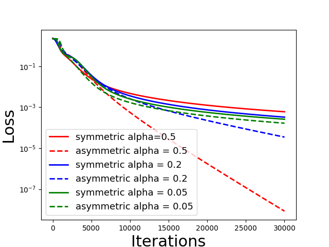
Figure 3: Comparisons between asymmetric and symmetric matrix sensing with different initialization scales. The dashed line represents the asymmetric matrix sensing, and the solid line represents the symmetric matrix sensing. Different color represents the different initialization scales.

I.2 Well-Conditioned Case and Ill-Conditioned Case

We run experiments with different conditional numbers of the ground-truth matrix. The conditional number $\kappa$ is selected as $\kappa=1.5,3$ and $10$. The minimum eigenvalue is selected by $0.66,0.33$ and $0.1$ respectively. The experiment results are shown in Figure 4

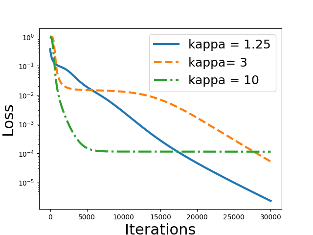
Figure 4: Comparisons between different conditional numbers

From the experiment results, we can see two phenomena:

$\bullet$ When the minimum eigenvalue is smaller, the gradient descent will converge to a smaller error at a linear rate. We call this phase the local convergence phase.

$\bullet$ After the local convergence phase, the curve first remains flat and then starts to converge at a linear rate again. We can see that the curve remains flat for a longer time when the matrix is ill-conditioned, i.e. $\kappa$ is larger.

This phenomenon has been theoretically identified by the previous work for the incremental learning (Jiang et al., 2022; Jin et al., 2023), in which GD is shown to sequentially recover singular components of the ground truth from the largest singular value to the smallest singular value.

I.3 Larger Initialization Scale

We also run experiments with a larger initialization scale $\alpha.$ The experiment results are shown in Figure 5. We find that if $\alpha$ is overly large, i.e. $\alpha=3$ and $5$, the algorithm actually converges slower and even fails to converge. This is reasonable since there is an upper bound requirement Eq. (20) for $\alpha$ in Theorem 8.

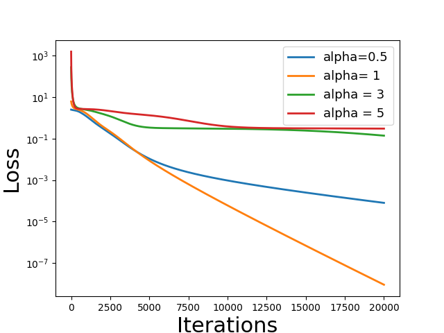
Figure 5: Comparisons between different large initialization scales

I.4 Larger True Rank and Over-Parameterized Rank

We run experiments with larger configurations $n=50,k=10$ and $r=5$. We use $m=2000$ samples. The experiment results are shown in Figure 6. We show that similar phenomena of symmetric and asymmetric cases also hold for a larger rank of the true matrix and a larger over-parameterized rank. Moreover, our new method also performs well in this setting.

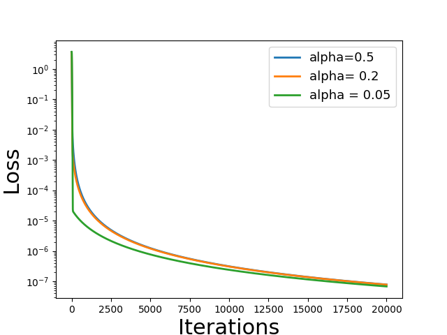
(a) Symmetric case

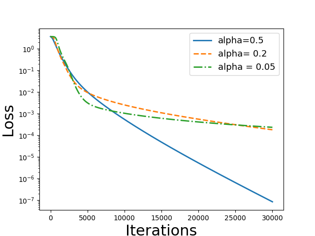
(b) Asymmetric Case

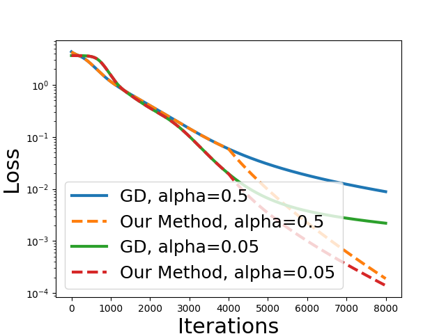
(c) Our new method

Figure 6: Experiment Results of larger true rank $r=5$ and over-parameterized rank $k=10$.

I.5 Initialization Phase

If we use GD with small initialization, GD always goes through an initialization phase where the loss is relatively flat, and then converges rapidly to a small error. In this subsection, we plot the first 5000 episodes of Figure 2(b). After zooming into the first 5000 iterations, we find the existence of the initialization phase. That is, the loss is rather flat during this phase. We can also see that the initialization phase is longer when $\alpha$ is smaller. The experiment results are shown in Figure 7.

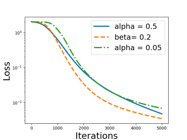
Figure 7: First 5000 episodes of Figure 2(b)

References

- Allen-Zhu et al. (2019) Zeyuan Allen-Zhu, Yuanzhi Li, and Yingyu Liang. Learning and generalization in overparameterized neural networks, going beyond two layers. Advances in neural information processing systems, 32, 2019.
- Arora et al. (2019) Sanjeev Arora, Nadav Cohen, Wei Hu, and Yuping Luo. Implicit regularization in deep matrix factorization. Advances in Neural Information Processing Systems, 32, 2019.
- Bhojanapalli et al. (2016) Srinadh Bhojanapalli, Anastasios Kyrillidis, and Sujay Sanghavi. Dropping convexity for faster semi-definite optimization. In Conference on Learning Theory, pp. 530–582. PMLR, 2016.
- Bi et al. (2022) Yingjie Bi, Haixiang Zhang, and Javad Lavaei. Local and global linear convergence of general low-rank matrix recovery problems. In Proceedings of the AAAI Conference on Artificial Intelligence, volume 36, pp. 10129–10137, 2022.
- Candes & Recht (2012) Emmanuel Candes and Benjamin Recht. Exact matrix completion via convex optimization. Communications of the ACM, 55(6):111–119, 2012.
- Candes & Plan (2011) Emmanuel J Candes and Yaniv Plan. Tight oracle inequalities for low-rank matrix recovery from a minimal number of noisy random measurements. IEEE Transactions on Information Theory, 57(4):2342–2359, 2011.
- Chen et al. (2012) Chih-Fan Chen, Chia-Po Wei, and Yu-Chiang Frank Wang. Low-rank matrix recovery with structural incoherence for robust face recognition. In 2012 IEEE conference on computer vision and pattern recognition, pp. 2618–2625. IEEE, 2012.
- Chizat et al. (2019) Lenaic Chizat, Edouard Oyallon, and Francis Bach. On lazy training in differentiable programming. Advances in neural information processing systems, 32, 2019.
- Davenport & Romberg (2016) Mark A Davenport and Justin Romberg. An overview of low-rank matrix recovery from incomplete observations. IEEE Journal of Selected Topics in Signal Processing, 10(4):608–622, 2016.
- Du et al. (2017) Simon S Du, Chi Jin, Jason D Lee, Michael I Jordan, Aarti Singh, and Barnabas Poczos. Gradient descent can take exponential time to escape saddle points. Advances in neural information processing systems, 30, 2017.
- Du et al. (2018a) Simon S Du, Wei Hu, and Jason D Lee. Algorithmic regularization in learning deep homogeneous models: Layers are automatically balanced. Advances in neural information processing systems, 31, 2018a.
- Du et al. (2018b) Simon S Du, Xiyu Zhai, Barnabas Poczos, and Aarti Singh. Gradient descent provably optimizes over-parameterized neural networks. arXiv preprint arXiv:1810.02054, 2018b.
- Dwivedi et al. (2020) Raaz Dwivedi, Nhat Ho, Koulik Khamaru, Martin J Wainwright, Michael I Jordan, and Bin Yu. Singularity, misspecification and the convergence rate of em. 2020.
- Fang et al. (2021) Cong Fang, Jason Lee, Pengkun Yang, and Tong Zhang. Modeling from features: a mean-field framework for over-parameterized deep neural networks. In Conference on learning theory, pp. 1887–1936. PMLR, 2021.
- Ge et al. (2017) Rong Ge, Chi Jin, and Yi Zheng. No spurious local minima in nonconvex low rank problems: A unified geometric analysis. In International Conference on Machine Learning, pp. 1233–1242. PMLR, 2017.
- Jacot et al. (2018) Arthur Jacot, Franck Gabriel, and Clément Hongler. Neural tangent kernel: Convergence and generalization in neural networks. Advances in neural information processing systems, 31, 2018.
- Jiang et al. (2022) Liwei Jiang, Yudong Chen, and Lijun Ding. Algorithmic regularization in model-free overparametrized asymmetric matrix factorization. arXiv preprint arXiv:2203.02839, 2022.
- Jin et al. (2017) Chi Jin, Rong Ge, Praneeth Netrapalli, Sham M Kakade, and Michael I Jordan. How to escape saddle points efficiently. In International conference on machine learning, pp. 1724–1732. PMLR, 2017.
- Jin et al. (2023) Jikai Jin, Zhiyuan Li, Kaifeng Lyu, Simon Shaolei Du, and Jason D Lee. Understanding incremental learning of gradient descent: A fine-grained analysis of matrix sensing. In International Conference on Machine Learning, pp. 15200–15238. PMLR, 2023.
- Li et al. (2019) Xingguo Li, Junwei Lu, Raman Arora, Jarvis Haupt, Han Liu, Zhaoran Wang, and Tuo Zhao. Symmetry, saddle points, and global optimization landscape of nonconvex matrix factorization. IEEE Transactions on Information Theory, 65(6):3489–3514, 2019.
- Li et al. (2018) Yuanzhi Li, Tengyu Ma, and Hongyang Zhang. Algorithmic regularization in over-parameterized matrix sensing and neural networks with quadratic activations. In Conference On Learning Theory, pp. 2–47. PMLR, 2018.
- Li et al. (2020) Zhiyuan Li, Yuping Luo, and Kaifeng Lyu. Towards resolving the implicit bias of gradient descent for matrix factorization: Greedy low-rank learning. arXiv preprint arXiv:2012.09839, 2020.
- Liu et al. (2012) Guangcan Liu, Zhouchen Lin, Shuicheng Yan, Ju Sun, Yong Yu, and Yi Ma. Robust recovery of subspace structures by low-rank representation. IEEE transactions on pattern analysis and machine intelligence, 35(1):171–184, 2012.
- Lu et al. (2020) Yiping Lu, Chao Ma, Yulong Lu, Jianfeng Lu, and Lexing Ying. A mean field analysis of deep resnet and beyond: Towards provably optimization via overparameterization from depth. In International Conference on Machine Learning, pp. 6426–6436. PMLR, 2020.
- Ma et al. (2021) Cong Ma, Yuanxin Li, and Yuejie Chi. Beyond procrustes: Balancing-free gradient descent for asymmetric low-rank matrix sensing. IEEE Transactions on Signal Processing, 69:867–877, 2021.
- Ma & Fattahi (2021) Jianhao Ma and Salar Fattahi. Sign-rip: A robust restricted isometry property for low-rank matrix recovery. arXiv preprint arXiv:2102.02969, 2021.
- Ma & Fattahi (2023) Jianhao Ma and Salar Fattahi. Global convergence of sub-gradient method for robust matrix recovery: Small initialization, noisy measurements, and over-parameterization. Journal of Machine Learning Research, 24(96):1–84, 2023.
- Nguyen & Pham (2020) Phan-Minh Nguyen and Huy Tuan Pham. A rigorous framework for the mean field limit of multilayer neural networks. arXiv preprint arXiv:2001.11443, 2020.
- Peng et al. (2014) Yigang Peng, Jinli Suo, Qionghai Dai, and Wenli Xu. Reweighted low-rank matrix recovery and its application in image restoration. IEEE transactions on cybernetics, 44(12):2418–2430, 2014.
- Recht et al. (2010) Benjamin Recht, Maryam Fazel, and Pablo A Parrilo. Guaranteed minimum-rank solutions of linear matrix equations via nuclear norm minimization. SIAM review, 52(3):471–501, 2010.
- Richert et al. (2022) Frederieke Richert, Roman Worschech, and Bernd Rosenow. Soft mode in the dynamics of over-realizable online learning for soft committee machines. Physical Review E, 105(5):L052302, 2022.
- Safran & Shamir (2018) Itay Safran and Ohad Shamir. Spurious local minima are common in two-layer relu neural networks. In International conference on machine learning, pp. 4433–4441. PMLR, 2018.