Differentially Encoded Observation Spaces
for Perceptive Reinforcement Learning

Abstract

Perceptive deep reinforcement learning (DRL) has lead to many recent breakthroughs for complex AI systems leveraging image-based input data. Applications of these results range from super-human level video game agents to dexterous, physically intelligent robots. However, training these perceptive DRL-enabled systems remains incredibly compute and memory intensive, often requiring huge training datasets and large experience replay buffers. This poses a challenge for the next generation of field robots that will need to be able to learn on the edge in order to adapt to their environments. In this paper, we begin to address this issue through differentially encoded observation spaces. By reinterpreting stored image-based observations as a video, we leverage lossless differential video encoding schemes to compress the replay buffer without impacting training performance. We evaluate our approach with three state-of-the-art DRL algorithms and find that differential image encoding reduces the memory footprint by as much as 14.2$\times$ and 16.7$\times$ across tasks from the Atari 2600 benchmark and the DeepMind Control Suite (DMC) respectively. These savings also enable large-scale perceptive DRL that previously required paging between flash and RAM to be run entirely in RAM, improving the latency of DMC tasks by as much as 32%.

I INTRODUCTION

With its ability to synthesize complex behaviors in both simulated and real environments, deep reinforcement learning (DRL) has been applied to solve a host of robotic-specific problems ranging from dexterous manipulation [1], to quadrupedal locomotion [2], to high-speed drone racing [3], as well as more general artificial intelligence (AI) feats of mastering tabletop [4] and competitive video games such as Dota 2 [5] and Minecraft [6].

Despite these achievements, DRL remains very sample inefficient, often requiring massive amounts of training data to learn. Because much of this persistent data is loaded into experience replay buffers during training, DRL is extremely memory intensive, limiting the number of computational platforms that can support such operations, and largely confining state-of-the-art model training to the cloud.

Interestingly, it is the observations in the replay buffer which often consume the majority of the memory, reaching over 90% for proprioceptive models [7]. The recent interest in perceptive DRL models [6, 8] only further exacerbates this problem. For example, as compared to the 224 bytes needed to store the proprioceptive observation space for the DeepMind Control Suite (DMC) [9] quadruped, a single 84x84 grayscale image requires over 7kB of memory. Consequently, deployment to the edge is unrealistic for such approaches. Still, many robots, especially those involved in tasks as consequential as search-and-rescue and space exploration [10], will have to adapt to ever-changing environmental conditions and continue to optimize and update their internal policies over the course of their lifetime [11], often in remote areas without access to fast network connections. As such, approaches that reduce the overall memory footprint of perceptive DRL are needed to enable edge deployments.

In this paper, we begin to address this issue through differentially encoded observation spaces. That is, by reinterpreting stored image-based observations as a video, we leverage lossless differential video encoding schemes to compress the replay buffer without impacting training performance. We evaluate our approach across ten Atari 2600 benchmark tasks [12] as well as two robotic control tasks from within the DMC, using three state-of-the-art DRL algorithms. We find that differential image encoding reduces the memory footprint by as much as 14.2$\times$ and 16.7$\times$ for the Atari and DMC tasks respectively. These savings also enable large-scale DRL that previously required paging between flash and RAM to be run entirely in RAM, improving latency for the DMC tasks by as much as 32%. We release our software and experiments open-source at: github.com/A2R-Lab/DiffCompressDRL.

II RELATED WORK

Perceptive DRL: Perceptive or image-based control and deep reinforcement learning (DRL) share common roots. First proposed a decade ago, Deep Q-Networks (DQNs) [13] bridged the gap between deep learning and RL, achieving super-human performance on many Atari 2600 video games using only visual input. Many model-free, DQN-based variants have followed [14, 15], further improving game-playing performance directly from pixel observations. Still, these early model-free methods remained quite data expensive. To address this, some turned to model-based or world-model learning in both the Atari [16] as well as robotic control [6, 17] domains. More recently, model-free methods have improved sample efficiency further through contrastive learning [18] and image augmentation [19]. Despite these improvements, perceptive DRL remains memory intensive, owing especially to the large size of image observations. For memory constrained systems and more complex tasks that require larger replay buffers, it has become necessary to store observations directly on disk, increasing the average memory access time and thus overall model training times [8].

Compressed Perceptive DRL: While recent image-based, model-free DRL methods have improved performance and sample efficiency through data augmentation [20], contrastive learning [18], and more robust latent observation space representations [21], little work has been done (aside from moving from RGB to grayscale [22]) to reduce the size of the stored image observations. Model-based methods offer an alternative by learning a world-model directly, thereby reducing the dependence on large amounts of replay experience [23, 24]. While these methods do show promise in highly complex simulated environments [6] as well as in some real laboratory settings [25], world-model learning tends to still struggle when the underlying world dynamics become highly complex [26]. For this reason, model-free methods remain popular for robotics applications leveraging learning in the real world [27].

Video Encoding for Learning: Traditionally, video encoding schemes aim to reduce the visual redundancy in digital video files without impacting human-perceived quality [28]. Modern video encoding standards such as MPEG-4 [29] and H.264 [30] use both intra- and inter-picture compression techniques to achieve this result. With the recent proliferation of deep learning for computer vision, some have begun optimizing traditional video encoding standards for learning frameworks [31]. While these methods have been applied to classification [32], object detection [33], and instance segmentation [34] tasks among others, little has been done to incorporate video compression within DRL.

III BACKGROUND

III-A Reinforcement Learning

Reinforcement learning poses problems as Markov decision processes (MDPs), where an MDP is defined by a set of observed and hidden states, $\mathcal{S}$, actions, $\mathcal{A}$, stochastic dynamics, $p(s_{t+1}|s_{t},a_{t})$, a reward function $r(s,a)$, and a discount factor, $\gamma$. The RL objective is to compute the policy, $\pi^{*}(s,a)$, that maximizes the expected discounted sum of future rewards, $\mathbb{E}_{s,a}\left(\sum_{t}\gamma^{t}r_{t}\right)$.

Perceptive RL, where states $s$ are represented by images, adds an additional caveat to the RL problem formulation, as representing a state using a single image rendering of the system is often not sufficiently descriptive [8]. To alleviate this issue, states are approximated by concatenating together the $f$ immediately preceding image frames $s_{t}=\{o_{t-f+1},\dots,o_{t}\}$, where $o_{t}$ is the image observation at timestep $t$ [13].

DRL algorithms parameterize the solution to these large MDPs with neural networks. In this work, we leverage three different state-of-the-art DRL algorithms: Proximal Policy Optimization [35], Quantile Regression DQN [15], and Data-regularized Q-v2 [8]. In the remainder of this section, we provide more detail on each algorithm.

III-A1 Proximal Policy Optimization (PPO)

Proximal Policy Optimization [35] is an on-policy, policy gradient [36] algorithm that employs an actor-critic framework to learn both the optimal policy, $\pi^{*}(s,a)$, as well as the optimal value function, $V^{*}(s)$. Both the policy $\pi_{\theta}$ and value function $V_{\phi}$ are parameterized by neural networks with weights $\theta$ and $\phi$ respectively. During training, PPO needs to store the parameters of both its value and policy networks–usually shallow multilayer perceptrons (MLPs)–as well as its on-policy rollout buffer $\mathcal{D}_{k}$. $\mathcal{D}_{k}$ stores $(s,a,r)$ tuples, which are refreshed during each iteration of the algorithm.

III-A2 Quantile Regression DQN (QR-DQN)

Quantile Regression DQN [15] improves upon the highly influential Deep Q-Networks (DQN) [13] algorithm, which uses experience replay to learn an optimal Q-function approximated by a neural network $Q_{\theta}$. While in the original DQN paper the authors train using a Huber loss [37] to maximize mean return, QR-DQN uses a custom quantile Huber loss in order to learn a distribution over expected returns. With this change, QR-DQN is able to significantly outperform DQN on a benchmark of Atari 2600 games. Unlike PPO, QR-DQN stores collected experience across all iterations in a much larger replay buffer $\mathcal{D}$, functioning as a size limited queue.

III-A3 Data-regularized Q-v2 (DrQ-v2)

Data-regularized Q-v2 [8] improves upon the Data-regularized Q [19] model-free RL algorithm. Both algorithms use data augmentation in conjunction with an actor-critic learning method in order to perform image-based continuous control. DrQ-v2 applies image augmentation through random shifts and then passes the augmented images through an encoder network $f_{\xi}$ to produce the final observations, which are used by an actor-critic DDPG [38] setup to learn the solution policy. DrQ-v2 achieves state-of-the-art model-free results on the DeepMind Control Suite, rivaling the performance of the popular model-based DreamerV2 [24], while doing so 4$\times$ faster (in terms of wall-clock training time). Like QR-DQN, DrQ-v2 stores its collected experience data in a large replay buffer $\mathcal{D}$.

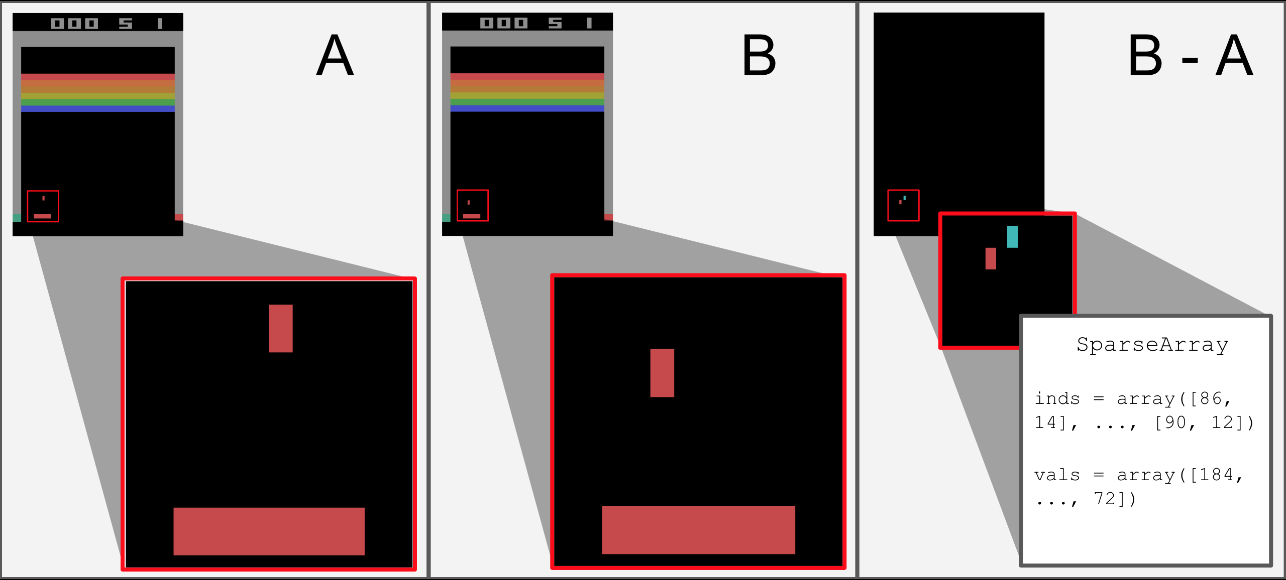
Figure 1: A graphical example of a differential image encoding taken from the Breakout Atari 2600 environment [12]. The two images, A and B shown on the left and middle, are very similar. The only difference in the resulting B-A image, shown on the right, occurs for the two different locations of the falling object. We can therefore encode this small difference in a highly compressed sparse matrix format.

III-B Memory Requirements for Perceptive DRL

Previous work showed that for proprioceptive DRL, the memory requirements for PPO were dominated by the observation space, consuming over 90% of the total memory [7]. Perceptive DRL does not change this and actually only makes matters worse. For example, the DMC quadruped requires only 224 bytes for a single proprioceptive observation, while a single 84x84 grayscale image requires over 7kB of memory. For the off-policy QR-DQN as well as DrQ-v2, an even greater percentage of the overall memory requirement is dominated by the observation space since, as mentioned above, their replay buffers are generally orders of magnitude larger than PPO’s rollout buffer.

III-C Differential Video Encoding

Modern video coding formats and codecs, like the H.264 [30] standard, make use of a number of compression and quantization techniques in order to reduce the overall size of video streams while preserving quality. One of the compression techniques employed is differential encoding (DE) [39], which can be used to compress both single images as well as multiple subsequent image frames by encoding the difference in inter-pixel or pixel-block values/intensities. In this work, we make use of a simplified version of differential video encoding–with inspiration from standard text-based DE used by most version control systems [40]–in order to compress the pixel-based observations found in rollout and replay buffers. We present our encoding scheme in detail in the following section.

IV METHOD

In this section, we detail a custom, lossless compression technique for image-based observation spaces. While we later show empirical results using PPO, QR-DQN, and DrQ-v2, we note that this differential encoding-based scheme can be applied to any image-based RL method in order to reduce the size of its stored observations.

IV-A Differential Encoder

During DRL training, there tends to be a level of temporal sortedness in experience replay buffers [41, 42], owing to the fact that many model-free RL algorithms add experience $(s,a,r)$ sequentially as they train. Therefore, while two states $s_{i},s_{j}$ drawn at random from a replay buffer may differ dramatically, two adjacent states $s_{i-1},s_{i}$ have a high likelihood of being similar, as they may originate from the same episode, just one control step apart. Applied to image-based observations, this means that images $o_{i-1}$ and $o_{i}$ will tend to be visually quite similar.

This similarity between adjacent image frames allows for a natural differential encoding-based compression scheme (Figure 1), which takes the difference between $o_{i}-o_{i-1}$ and stores the result in sparse matrix format $S_{i}=\texttt{SparseArray}(o_{i}-o_{i-1})$. To decode $o_{i}$, it is then only necessary to store $o_{i-1}$ and $S_{i}$, as:

$$o_{i}=o_{i-1}+S_{i}.$$ (1)

In order to efficiently store and access these image differences, we define a custom sparse matrix implementation SparseArray that stores all nonzero pixels using two arrays inds and vals, where inds stores pixel locations and vals stores pixel values. Because image observations in both the Atari 2600 benchmark and DeepMind Control Suite are stored as 84x84, 8-bit unsigned integer arrays (assuming grayscale images), we let inds store 8-bit unsigned integers and vals store 16-bit signed integers. Assuming $o_{i}-o_{i-1}$ results in $n$ nonzero pixel values, we can store a 7kB input image in $4n$ bytes.

While it is possible that $o_{i}-o_{i-1}$ results in an image with a majority nonzero pixel values, in practice we find the number of nonzero pixels $n$ to be small. Nevertheless, we handle this corner case explicitly in SparseArray. If $4n>84\times 84$, we store the full image array in order to cap the maximum image size at 7kB.

IV-B Observation Indexing

As noted in the previous section, image-based learning methods generally store states $s$ as a stack of the $f$ prior image observations. Letting $f=4$ (as is the case for our Atari 2600 experiments in Section V), this results in each state taking up $84\times 84\times 4=28$kB of memory.

Instead of storing states in this full image stack format, we define two separate arrays obs, which stores the individual image observations, and obs_inds, which stores pointers into obs for each state. To reconstruct the full state $s_{i}$, we simply concatenate the individual observations referenced by $\texttt{obs\_inds}_{i}$. In most cases $\texttt{obs\_inds}_{i}=\{(i-f+1),(i-f+2),\dots,i\}$ resulting in:

$$s_{i}=\{\texttt{obs}_{(i-f+1)},\texttt{obs}_{(i-f+2)},\dots,\texttt{obs}_{i}\}.$$ (2)

However, in various corner cases, this is not the case, necessitating the use of the pointer array. For example, for the first few observations, at the start of an episode, individual observations need to be repeated to fill a history of size $f$.

Through observation indexing alone, we can reduce the memory required to store all states by almost $f\times$, as $f$ pointers are a fraction of the size of the $(f-1)$ image observations we no longer need to save.

IV-C Observation Compressor

With both the differential image encoder and smart observation indexing, we can define an observation compressor to handle the storage and retrieval of image-based observations. Following best practices from the video encoding literature, we apply our approach to each set of $f$ images.

Our compressor, ObsComp, internally stores three arrays: obs, sparse_obs, and obs_inds. Using these arrays we can then define the following two operations: ObsComp.get(i) and ObsComp.set(s, i), which get and set the uncompressed state $s_{i}$ respectively.

To set a state $s_{i}$, we first compute the observation index array $\texttt{obs\_inds}_{i}=\{(i-f+1),\dots,i\}$. Next, we check if $i\mod f=0$, and if so store the raw image frame $\texttt{obs}_{i/f}=o_{i}$. If not, we compute and store the SparseArray, $\texttt{sparse\_obs}_{i/f,(i\mod f)-1}=o_{i}-\texttt{obs}_{i-i\mod f}$.

To get a state $s_{i}$, we retrieve the observation indices $\texttt{obs\_inds}_{i}$ and concatenate the individual frames referenced either directly from obs or from decoding compressed frames stored in sparse_obs (Equation 1).

IV-D Theoretical Compression Factor

With these definitions in mind, we can evaluate the theoretical compression factor for our approach, that is the reduction ratio in overall memory consumption.

Let obs store uncompressed image observations $o_{i}$ and be of shape $(d,I,I)$, where $d=|\mathcal{D}|/f$ is the size of the uncompressed replay buffer divided by the frame stack size $f$, and $(I,I)$ is the size of a single grayscale input image.

Let sparse_obs store compressed image observations $S_{i}$ in SparseArray format and be of shape $(d,f-1)$. Note that each element of this array contains the overhead to store a pointer to a SparseArray object, which can then be accessed to perform observation decompression (Equation 1).

Finally, let obs_inds store frame stack indices (as explained in the previous sub-section) and be of shape $(|\mathcal{D}|,f)$.

Assuming each $S_{i}$ incurs an overhead of an 8-byte pointer and $N$ is the number of total nonzero pixel values for all $S_{i}\in\texttt{sparse\_obs}$, we can define the memory size of ObsComp as the following (in bytes):

$$I^{2}d+8d(f-1)+4N+4|\mathcal{D}|f.$$ (3)

In comparison, to store all observations without any form of compression would take $|\mathcal{D}|\times I\times I\times f$ bytes. Overall, our method yields a theoretical compression factor of:

$$\frac{I^{2}|\mathcal{D}|f}{I^{2}d+8d(f-1)+4N+4|\mathcal{D}|f}.$$ (4)

Letting $N=d(f-1)n$, where $n$ is the average number of pixels that need to be stored per compressed image, and $I=84$ (as used in our experiments in Section V), we can further simplify the compression factor in terms of $f$ and $n$:

$$\frac{1764f}{(1762-n)/f+2+n}.$$ (5)

Noting that $n=I^{2}\phi=7056\phi$, where $\phi$ is the average percentage of pixels that need to be stored per compressed image, we plot the theoretical compression factor resulting from our approach for varying values of $f$ and $\phi$ in Figure 2. We observe that even with a relatively small frame stack length of $f=4$, an order of magnitude compression factor can still be achieved as long as at most an average of 5% of the pixels remain in the encoded images. Similarly, with a larger frame stack length of $f=10$, we can also still achieve an order of magnitude compression factor, even with up to 25% of the pixels remaining.

Figure 2: Theoretical compression factor for different values of frame stack length $f$ and average percent of total pixels remaining per compressed image $\phi$. Higher values correspond to more compression achieved.

V EXPERIMENTS AND RESULTS

We evaluate the effectiveness of our differential encoder-based compression framework using tasks from both the Atari 2600 benchmark [12] as well as the DeepMind Control Suite (DMC) [9]. We analyze our results in terms of training speed, memory consumption (and associated compression factor), and convergence performance. Our full implementation, including values for all hyperparameters used in our experiments, can be found in our open-source GitHub repository at: github.com/A2R-Lab/DiffCompressDRL.

V-A Methodology

For all Atari benchmark tasks, we set $f$ to the default value of $4$ and train using two popular on- and off-policy reinforcement learning algorithms: Proximal Policy Optimization (PPO) [35] and Quantile Regression DQN (QR-DQN) [15]. We use publicly available implementations of both PPO and QR-DQN (credit: stable-baselines3 [43]), modifying only the buffer logic in order to accommodate observation compression. For the DeepMind Control Suite tasks, we set $f$ to the default value of $3$ and train on a state-of-the-art off-policy, data augmentation-based reinforcement learning algorithm: Data-regularized Q-v2 (DrQ-v2) [8]. We use Meta Research’s official implementation of DrQ-v2, again only modifying logic pertaining to the storage and retrieval of image observations. Unless otherwise noted, we run all experiments using the default PPO, QR-DQN, and DrQ-v2 hyperparameters. Exact values for all hyperparameters can be found on our GitHub repository.

Comp Type	Env	FPS (base)	FPS (ours)	GB (base)	GB (ours)	Total Comp
	Walker	119	142	63.5	7.1	8.9$\times$
Half	Quadruped	184	243	63.6	7.1	9.0$\times$
	AVG	152	193	63.6	7.1	9.0$\times$
	Walker	119	73	63.5	3.8	16.7$\times$
Full	Quadruped	184	135	63.6	4.1	15.5$\times$
	AVG	152	104	63.6	4.0	15.9$\times$

TABLE I: DrQ-v2 training speed (FPS), replay buffer size (GB), and total memory reduction due to compression (Total Comp) of both speed-optimized (Half) and memory-optimized (Full) compression for the DMC [9] tasks of Walker Walk and Quadruped Walk.

V-B Robotic Control Tasks

In this section, we evaluate our approach on the Walker Walk and Quadruped Walk tasks from the DMC robotic control suite [9]. We define two separate levels of image-based compression: Half and Full. Half, or speed-optimized compression uses a fully vectorized implementation of observation indexing (Section IV-B) but does not leverage observation compression (Section IV-C), while Full uses the entire compression stack detailed in Section IV, but as a result, does not support vectorization. In addition, both implementations store all experience values in our replay buffer directly in memory, unlike DrQ-v2, which by default needs to store such values to disk.

Table I compares the training speed, replay buffer size, and total compression factor (Equation 4) achieved with Half and Full compression using DrQ-v2 across the Walker Walk and Quadruped Walk DMC tasks. We find that on average, Half and Full compression reduce the replay buffer’s memory footprint by 9$\times$ and 15.9$\times$ respectively, with Full achieving a 16.7$\times$ compression factor for Walker Walk.

In terms of training speed, our Half compression approach, which is fully vectorized, improves latency over the baseline DrQ-v2 implementation by as much as 32% while still achieving the aforementioned 9$\times$ compression factor. As noted earlier, our Full compression implementation does not yet leverage vectorization and so results in an average slow-down of 32% as compared to the baseline DrQ-v2 implementation, which, despite storing its replay buffer on disk, leverages multi-threaded data loaders and batch pre-fetching in order to be as low latency as possible.

Figure 3 plots the learning curves of DrQ-v2 across the Walker Walk and Quadruped Walk DMC environments using no compression (black), Half compression (light blue), and Full compression (dark blue). We average our results across five random seeds and display the standard deviation with the accompanying shaded region. As expected, given that our compression is lossless, we find convergence is not affected by our approach, as all final rewards both with and without differential encoder-based compression are well within a standard deviation of each other.

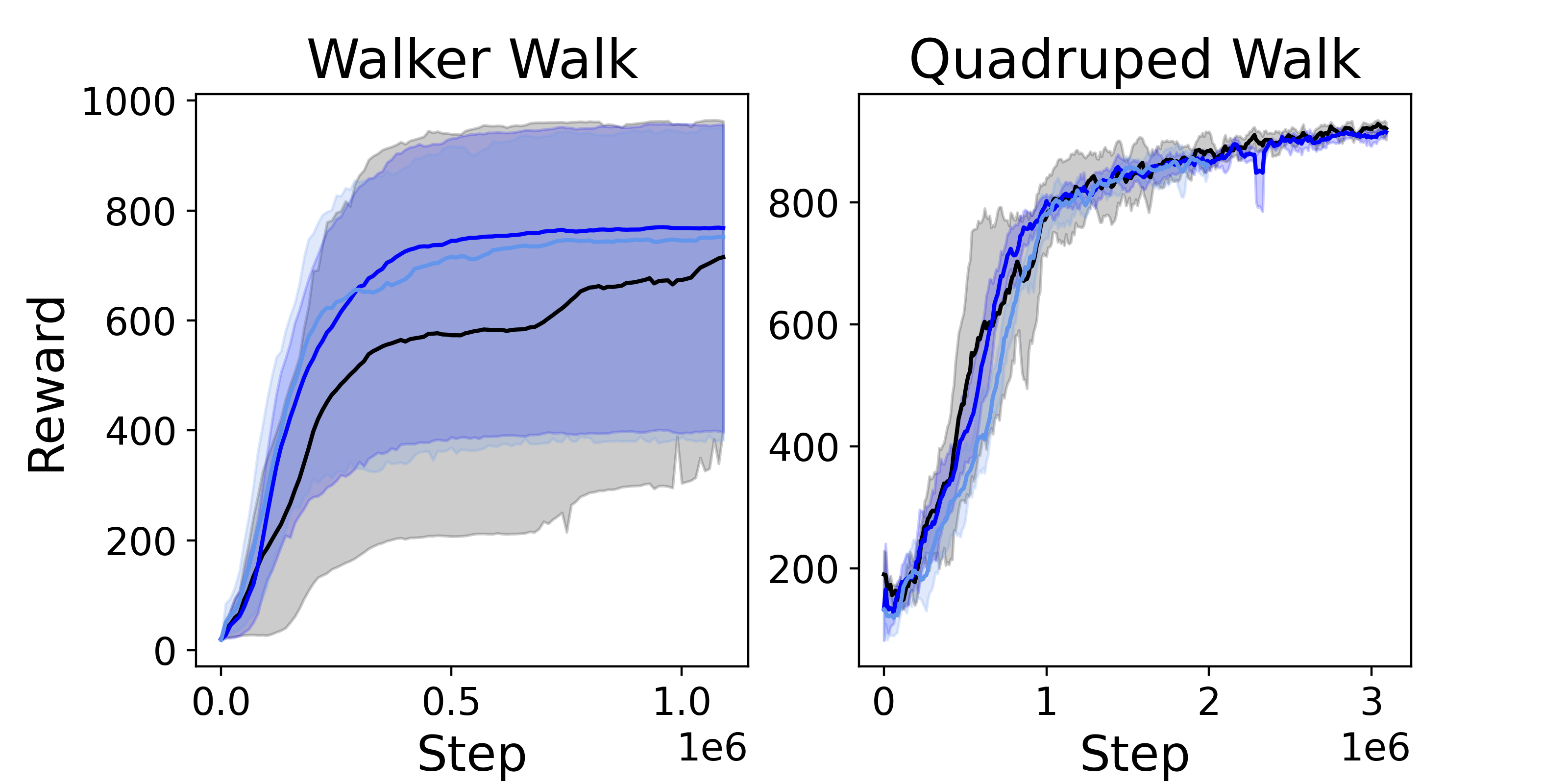
Figure 3: Learning curves of DrQ-v2 with Half (light blue), Full (dark blue), and no (black) compression for the DMC [9] tasks of Walker Walk and Quadruped Walk.

V-C Atari Environments

Table II compares the training speed and replay buffer size with and without differential encoding-based image compression across 10 Atari 2600 benchmark environments [12], as well as the compression factor, for both PPO and QR-DQN using the Full compression approach. We find that on average, Full compression is able to reduce the replay buffer’s memory footprint by 8.9$\times$ and 9.9$\times$ for PPO and QR-DQN respectively. While the end compression factor does vary by environment–as the number $N$ of nonzero pixel values stored in the observation compressor (Equation 3) differs depending on the level of inter-frame dissimilarity within the environment–we find that 5/10 PPO and 6/10 QR-DQN environments achieve over a 10$\times$ compression factor, with our best-case environments achieving as much as a 14.2$\times$ reduction. As previously noted, Full compression is not fully vectorized and can be optimized through future work, as such we find an average 5% and 29% slow-down for PPO and QR-DQN respectively as compared to the default, vectorized, stable-baselines3 implementation.

Figure 4 plots the learning curves of PPO and QR-DQN across the ten Atari environments for the first 10M steps of training. These figures report the average of five random seeds and also display the standard deviation with the accompanying shaded regions. As in the DMC environments, we find that convergence is not affected, with all final rewards being well within a standard deviation of one another.

Alg	Env	FPS (base)	FPS (ours)	MB (base)	MB (ours)	Total Comp
	Asteroids	1605	1535	27.6	2.6	10.8$\times$
	BeamRider	1339	1267	27.6	7.6	3.6$\times$
	Breakout	1437	1383	27.6	2.0	14.2$\times$
	Enduro	1117	1062	27.6	3.5	7.9$\times$
	MsPacman	1432	1389	27.6	2.3	12.1$\times$
PPO	Pong	1582	1512	27.6	2.0	13.9$\times$
	Qbert	1507	1452	27.6	3.0	9.1$\times$
	RoadRunner	1347	1267	27.6	3.0	9.0$\times$
	Seaquest	1466	1371	27.6	2.9	9.6$\times$
	SpaceInvaders	1468	1395	27.6	2.4	11.3$\times$
	AVG	1430	1363	27.6	3.1	8.9$\times$
	Asteroids	897	616	2694	265	10.2$\times$
	BeamRider	792	547	2694	552	4.9$\times$
	Breakout	833	587	2694	190	14.2$\times$
	Enduro	722	536	2694	306	8.8$\times$
	MsPacman	839	597	2694	219	12.3$\times$
DQN	Pong	881	627	2694	192	14.0$\times$
	Qbert	849	608	2694	213	12.7$\times$
	RoadRunner	808	576	2694	290	9.3$\times$
	Seaquest	732	484	2694	278	9.7$\times$
	SpaceInvaders	861	607	2694	227	11.9$\times$
	AVG	821	579	2694	273	9.9$\times$

TABLE II: Training speed in frames/steps per second (FPS), replay buffer size (MB), and total memory reduction due to compression (Total Comp) of both PPO and QR-DQN (DQN) across ten Atari 2600 [12] environments.

VI CONCLUSION AND FUTURE WORK

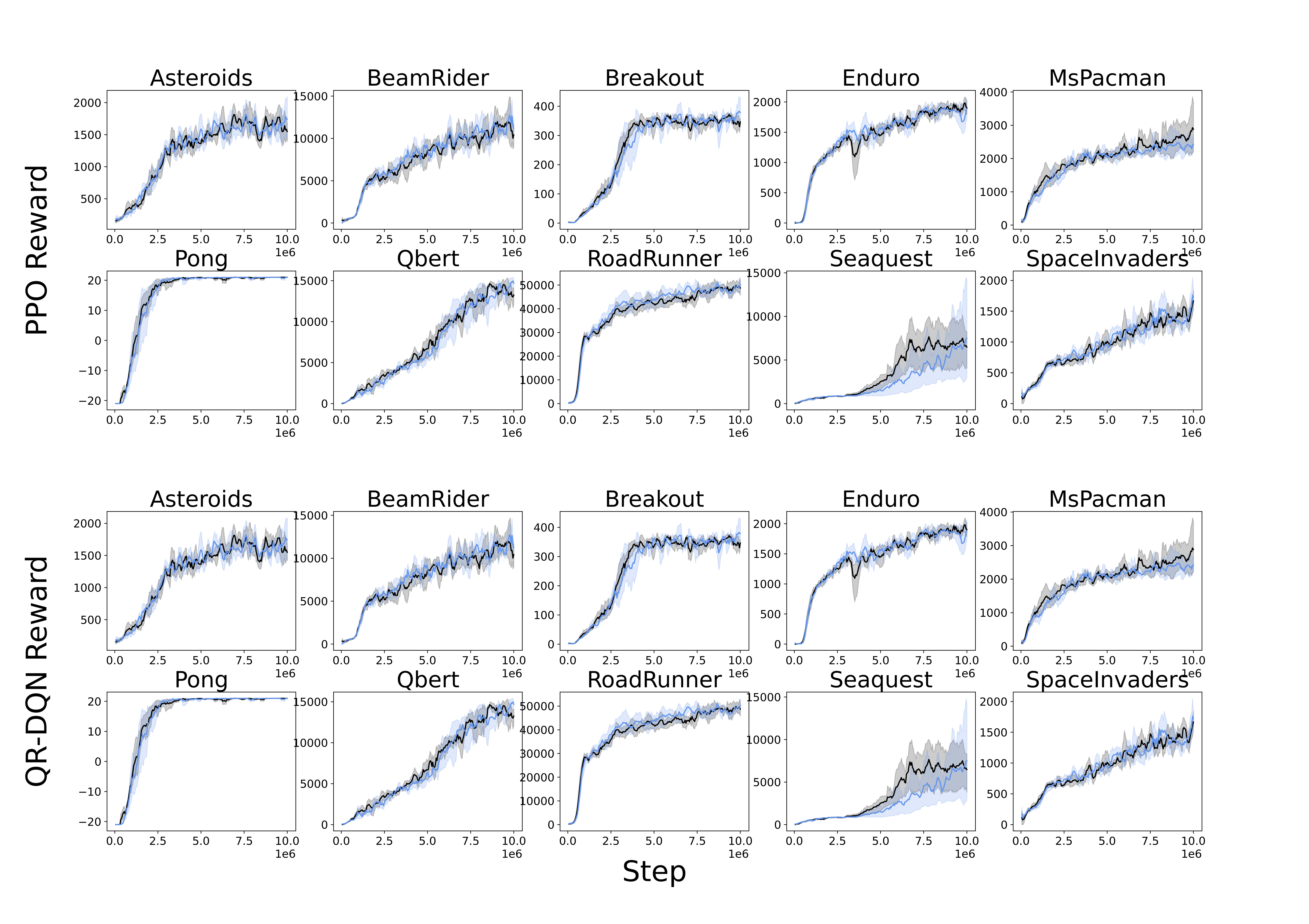
Figure 4: Learning curves of PPO (top) and QR-DQN (bottom) with (blue) and without (black) pixel-based compression across ten Atari 2600 [12] environments. Rewards are averaged across five trials and standard deviations are shaded.

This paper presents a novel, differential encoding-based method for observation compression, reducing the overall memory requirements of perceptive DRL without impacting training performance.

We evaluate the compression factor, training speed, and learning performance across ten Atari and two DMC tasks using three state-of-the-art on- and off-policy perceptive DRL algorithms. We find that differential image encoding reduces the memory footprint by as much as 14.2$\times$ and 16.7$\times$ for the Atari and DMC tasks respectively. These savings also enable large-scale DRL that previously required paging between flash and RAM to be run entirely in RAM, improving latency for the DMC tasks by as much as 27%.

Admittedly, not all learning-based approaches will benefit equally from observation compression. For instance, newer model-based techniques may trade off large replay buffers for more expressive world models [6]. However, if we are to realize lifelong, practical learning on the edge, curbing memory usage, wherever it may be, is essential.

In future work, we hope to further optimize our method through enhanced vectorization and parallelization in order to speed up training. Finally, we hope to deploy our compression technique onto physical robot hardware and test it in the context of both real-world edge RL and tiny robot learning [44]. We hope that this effort will aid in reducing cost and compute barriers for state-of-the-art RL across all robot platforms.

References

- [1] OpenAI, M. Andrychowicz, B. Baker, M. Chociej, R. Jozefowicz, B. McGrew, J. Pachocki, A. Petron, M. Plappert, G. Powell, A. Ray, J. Schneider, S. Sidor, J. Tobin, P. Welinder, L. Weng, and W. Zaremba, “Learning dexterous in-hand manipulation,” 2018. [Online]. Available: https://arxiv.org/abs/1808.00177
- [2] T. Miki, J. Lee, J. Hwangbo, L. Wellhausen, V. Koltun, and M. Hutter, “Learning robust perceptive locomotion for quadrupedal robots in the wild,” Science Robotics, vol. 7, no. 62, jan 2022. [Online]. Available: https://doi.org/10.1126%2Fscirobotics.abk2822
- [3] Y. Song, M. Steinweg, E. Kaufmann, and D. Scaramuzza, “Autonomous drone racing with deep reinforcement learning,” 2021. [Online]. Available: https://arxiv.org/abs/2103.08624
- [4] D. Silver, T. Hubert, J. Schrittwieser, I. Antonoglou, M. Lai, A. Guez, M. Lanctot, L. Sifre, D. Kumaran, T. Graepel, T. Lillicrap, K. Simonyan, and D. Hassabis, “Mastering chess and shogi by self-play with a general reinforcement learning algorithm,” 2017.
- [5] OpenAI, :, C. Berner, G. Brockman, B. Chan, V. Cheung, P. Dębiak, C. Dennison, D. Farhi, Q. Fischer, S. Hashme, C. Hesse, R. Józefowicz, S. Gray, C. Olsson, J. Pachocki, M. Petrov, H. P. d. O. Pinto, J. Raiman, T. Salimans, J. Schlatter, J. Schneider, S. Sidor, I. Sutskever, J. Tang, F. Wolski, and S. Zhang, “Dota 2 with large scale deep reinforcement learning,” 2019.
- [6] D. Hafner, J. Pasukonis, J. Ba, and T. Lillicrap, “Mastering diverse domains through world models,” 2023.
- [7] L. Grossman and B. Plancher, “Just round: Quantized observation spaces enable memory efficient learning of dynamic locomotion,” in IEEE International Conference on Robotics and Automation (ICRA), London, UK, May. 2023.
- [8] D. Yarats, R. Fergus, A. Lazaric, and L. Pinto, “Mastering visual continuous control: Improved data-augmented reinforcement learning,” 2021.
- [9] Y. Tassa, Y. Doron, A. Muldal, T. Erez, Y. Li, D. de Las Casas, D. Budden, A. Abdolmaleki, J. Merel, A. Lefrancq, T. Lillicrap, and M. Riedmiller, “Deepmind control suite,” 2018.
- [10] P. R. Gankidi and J. Thangavelautham, “Fpga architecture for deep learning and its application to planetary robotics,” in 2017 IEEE Aerospace Conference, 2017, pp. 1–9.
- [11] S. Thrun and T. M. Mitchell, “Lifelong robot learning,” Robotics and Autonomous Systems, vol. 15, no. 1, pp. 25–46, 1995, the Biology and Technology of Intelligent Autonomous Agents. [Online]. Available: https://www.sciencedirect.com/science/article/pii/092188909500004Y
- [12] M. G. Bellemare, Y. Naddaf, J. Veness, and M. Bowling, “The arcade learning environment: An evaluation platform for general agents,” Journal of Artificial Intelligence Research, vol. 47, pp. 253–279, jun 2013. [Online]. Available: https://doi.org/10.1613%2Fjair.3912
- [13] V. Mnih, K. Kavukcuoglu, D. Silver, A. Graves, I. Antonoglou, D. Wierstra, and M. Riedmiller, “Playing atari with deep reinforcement learning,” 2013.
- [14] M. Hessel, J. Modayil, H. van Hasselt, T. Schaul, G. Ostrovski, W. Dabney, D. Horgan, B. Piot, M. Azar, and D. Silver, “Rainbow: Combining improvements in deep reinforcement learning,” 2017.
- [15] W. Dabney, M. Rowland, M. G. Bellemare, and R. Munos, “Distributional reinforcement learning with quantile regression,” 2017.
- [16] L. Kaiser, M. Babaeizadeh, P. Milos, B. Osinski, R. H. Campbell, K. Czechowski, D. Erhan, C. Finn, P. Kozakowski, S. Levine, A. Mohiuddin, R. Sepassi, G. Tucker, and H. Michalewski, “Model-based reinforcement learning for atari,” 2020.
- [17] D. Hafner, T. Lillicrap, I. Fischer, R. Villegas, D. Ha, H. Lee, and J. Davidson, “Learning latent dynamics for planning from pixels,” 2019.
- [18] A. Srinivas, M. Laskin, and P. Abbeel, “Curl: Contrastive unsupervised representations for reinforcement learning,” 2020.
- [19] I. Kostrikov, D. Yarats, and R. Fergus, “Image augmentation is all you need: Regularizing deep reinforcement learning from pixels,” 2021.
- [20] M. Laskin, K. Lee, A. Stooke, L. Pinto, P. Abbeel, and A. Srinivas, “Reinforcement learning with augmented data,” 2020.
- [21] D. Yarats, R. Fergus, A. Lazaric, and L. Pinto, “Reinforcement learning with prototypical representations,” 2021.
- [22] M. Laskin, K. Lee, A. Stooke, L. Pinto, P. Abbeel, and A. Srinivas, “Reinforcement learning with augmented data,” 2020.
- [23] D. Hafner, T. Lillicrap, I. Fischer, R. Villegas, D. Ha, H. Lee, and J. Davidson, “Learning latent dynamics for planning from pixels,” 2018. [Online]. Available: https://arxiv.org/abs/1811.04551
- [24] D. Hafner, T. Lillicrap, M. Norouzi, and J. Ba, “Mastering atari with discrete world models,” 2022.
- [25] P. Wu, A. Escontrela, D. Hafner, K. Goldberg, and P. Abbeel, “Daydreamer: World models for physical robot learning,” 2022.
- [26] M. Tomar, U. A. Mishra, A. Zhang, and M. E. Taylor, “Learning representations for pixel-based control: What matters and why?” 2021.
- [27] W. Yu, D. Jain, A. Escontrela, A. Iscen, P. Xu, E. Coumans, S. Ha, J. Tan, and T. Zhang, “Visual-locomotion: Learning to walk on complex terrains with vision,” in Proceedings of the 5th Conference on Robot Learning, ser. Proceedings of Machine Learning Research, A. Faust, D. Hsu, and G. Neumann, Eds., vol. 164. PMLR, 08–11 Nov 2022, pp. 1291–1302. [Online]. Available: https://proceedings.mlr.press/v164/yu22a.html
- [28] D. Wood, “Task oriented video coding: A survey,” 2022.
- [29] T. Ebrahimi and C. Horne, “Mpeg-4 natural video coding – an overview,” Signal Processing: Image Communication, vol. 15, no. 4, pp. 365–385, 2000. [Online]. Available: https://www.sciencedirect.com/science/article/pii/S0923596599000545
- [30] J.-W. Chen, C.-Y. Kao, and Y.-L. Lin, “Introduction to h. 264 advanced video coding,” in Proceedings of the 2006 Asia and South Pacific Design Automation Conference, 2006, pp. 736–741.
- [31] W. Yang, H. Huang, Y. Hu, L.-Y. Duan, and J. Liu, “Video coding for machine: Compact visual representation compression for intelligent collaborative analytics,” 2021.
- [32] Z. Huang, C. Jia, S. Wang, and S. Ma, “Visual analysis motivated rate-distortion model for image coding,” 2021.
- [33] Z. Yang, Y. Wang, C. Xu, P. Du, C. Xu, C. Xu, and Q. Tian, “Discernible image compression,” in Proceedings of the 28th ACM International Conference on Multimedia. ACM, oct 2020. [Online]. Available: https://doi.org/10.1145%2F3394171.3413968
- [34] N. Le, H. Zhang, F. Cricri, R. Ghaznavi-Youvalari, and E. Rahtu, “Image coding for machines: an end-to-end learned approach,” in ICASSP 2021 - 2021 IEEE International Conference on Acoustics, Speech and Signal Processing (ICASSP). IEEE, jun 2021. [Online]. Available: https://doi.org/10.1109%2Ficassp39728.2021.9414465
- [35] J. Schulman, F. Wolski, P. Dhariwal, A. Radford, and O. Klimov, “Proximal Policy Optimization Algorithms,” arXiv:1707.06347 [cs], July 2017.
- [36] R. S. Sutton, D. M. A. llester, S. Singh, and Y. Mansour, “Policy Gradient Methods for Reinforcement Learning with Function Approximation,” 2000, pp. 1057–1063.
- [37] P. J. Huber, “Robust Estimation of a Location Parameter,” The Annals of Mathematical Statistics, vol. 35, no. 1, pp. 73 – 101, 1964. [Online]. Available: https://doi.org/10.1214/aoms/1177703732
- [38] T. P. Lillicrap, J. J. Hunt, A. Pritzel, N. Heess, T. Erez, Y. Tassa, D. Silver, and D. Wierstra, “Continuous control with deep reinforcement learning,” 2015. [Online]. Available: https://arxiv.org/abs/1509.02971
- [39] K. Sayood, “Chapter 11 - differential encoding,” in Introduction to Data Compression (Fifth Edition), fifth edition ed., ser. The Morgan Kaufmann Series in Multimedia Information and Systems, K. Sayood, Ed. Morgan Kaufmann, 2018, pp. 351–378. [Online]. Available: https://www.sciencedirect.com/science/article/pii/B9780128094747000112
- [40] N. B. Ruparelia, “The history of version control,” ACM SIGSOFT Software Engineering Notes, vol. 35, no. 1, pp. 5–9, 2010.
- [41] L.-J. Lin, “Self-improving reactive agents based on reinforcement learning, planning and teaching,” Machine Learning, vol. 8, no. 3, pp. 293–321, 1992. [Online]. Available: https://doi.org/10.1007/BF00992699
- [42] T. Schaul, J. Quan, I. Antonoglou, and D. Silver, “Prioritized experience replay,” 2016.
- [43] A. Raffin, A. Hill, A. Gleave, A. Kanervisto, M. Ernestus, and N. Dormann, “Stable-baselines3: Reliable reinforcement learning implementations,” Journal of Machine Learning Research, vol. 22, no. 268, pp. 1–8, 2021. [Online]. Available: http://jmlr.org/papers/v22/20-1364.html
- [44] S. M. Neuman, B. Plancher, B. P. Duisterhof, S. Krishnan, C. Banbury, M. Mazumder, S. Prakash, J. Jabbour, A. Faust, G. C. de Croon, and V. Janapa Reddi, “Tiny robot learning: Challenges and directions for machine learning in resource-constrained robots,” in 2022 IEEE International Conference on Artificial Intelligence Circuits and Systems (AICAS), Incheon, Korea, June 2022.