CausalTime: Realistically Generated Time-series for Benchmarking of Causal Discovery

Abstract

Time-series causal discovery (TSCD) is a fundamental problem of machine learning. However, existing synthetic datasets cannot properly evaluate or predict the algorithms’ performance on real data. This study introduces the CausalTime pipeline to generate time-series that highly resemble the real data and with ground truth causal graphs for quantitative performance evaluation. The pipeline starts from real observations in a specific scenario and produces a matching benchmark dataset. Firstly, we harness deep neural networks along with normalizing flow to accurately capture realistic dynamics. Secondly, we extract hypothesized causal graphs by performing importance analysis on the neural network or leveraging prior knowledge. Thirdly, we derive the ground truth causal graphs by splitting the causal model into causal term, residual term, and noise term. Lastly, using the fitted network and the derived causal graph, we generate corresponding versatile time-series proper for algorithm assessment. In the experiments, we validate the fidelity of the generated data through qualitative and quantitative experiments, followed by a benchmarking of existing TSCD algorithms using these generated datasets. CausalTime offers a feasible solution to evaluating TSCD algorithms in real applications and can be generalized to a wide range of fields. For easy use of the proposed approach, we also provide a user-friendly website, hosted on www.causaltime.cc.

1 Introduction

Inferring causal structures from time-series, i.e., time-series causal discovery (TSCD), is a fundamental problem in machine learning. It goes beyond prediction or forecasting by revealing the complex interactions buried under multi-variate time-series. Recently, many algorithms have been proposed [31; 29; 57; 5] and achieved satisfactory performance, i.e., the discovered causal graphs are close to the ground-truth counterparts. Under some settings, the causal discovery results are nearly perfect, with AUROC scores approaching 1.

However, the benchmarks for TSCD algorithms do not suffice for the performance evaluation. First of all, for the statistical significance of the quantitative evaluation results, the datasets need to be improved in terms of quality and quantity. Next, the current datasets are limited to several fields and do not cover wide application directions. More importantly, the datasets with ground-truth causal graphs are synthesized and might deviate from the true data-generating process, so the scores may not reflect the performance on real data [40].

Despite the fact that recent works also propose better benchmarks for time-series causal discovery [28; 44], as well as static settings [16; 10; 11]. Current TSCD algorithms often incorporate three types of datasets: Numerical datasets, e.g., VAR (vector auto-regression) and Lorenz-96 [24], are simulated using closed-form equations. Although some of these equations (Lorenz-96) are inspired by real application scenarios, e.g., climate dynamics, they are over-simplified and have very limited generalizability to real-world applications [44]. Quasi-real datasets are composed of time-series generated with manually designed dynamics that mimic real counterparts under a certain scenario. For example, DREAM3 [39] is a dataset simulated using gene expression and regulation dynamics, and NetSim [48] is generated by simulating interactions between human brain regions under observation of fMRI. The problem with this type of dataset is that it only covers a few research areas with underlying mechanisms relatively clearly known. For fields such as healthcare or finance, it is hard or even impossible to generate realistic time-series with manually designed dynamics. Real datasets (such as MoCap [53], S&P 100 stock returns [35]) do not have the above-mentioned problem, but the dealbreaker is that the ground truth causal graph is mostly inaccessible, and we have to resort to some ad hoc explanations. As shown in Table 1, currently available benchmarking tools cannot support a comprehensive evaluation of the time-series causal discovery algorithm. Therefore, an approach for generating benchmarks that highly mimic the real data in different scenarios and with true causal graphs is highly demanded.

Table 1: Comparison of benchmarks for time-series causal discovery evaluation.

Datasets	Numerical	Quasi-real	Real	CausalTime (Ours)
Realistic Data	Low	Moderate	Very High	High
With True Causal Graph	✓	✓	✗	✓
Generalizable to Diverse Fields	✗	✗	✓	✓

In this work, we propose a novel pipeline capable of generating realistic time-series along with a ground truth causal graph and is generalizable to different fields, named CausalTime. The process of generating time-series with a given causal graph can be implemented using the autoregression model, however, pursuing a causal graph that matches the target time-series with high accuracy is nontrivial, especially for the data with little prior knowledge about the underlying causal mechanism. To address this issue, we propose to use a deep neural network to fit the observed data with high accuracy, and then retrieve a causal graph from the network or from prior knowledge that holds high data fidelity. Specifically, we first obtain a hypothesized causal graph by performing importance analysis on the neural network or leveraging prior knowledge, and then split the functional causal model into causal term, residual term, and noise term. The split model can naturally generate time-series matching the original data observations well. It is worth noting that the retrieval of the causal graph is not a causal discovery process and does not necessarily uncover the underlying causal relationship, but can produce realistic time-series to serve as the benchmark of causal discovery algorithms.

Our benchmark is open-source and user-friendly, we host our website at www.causaltime.cc. Specifically, our contributions include:

• We propose CausalTime, a pipeline to generate realistic time-series with ground truth causal graphs, which can be applied to diverse fields and provide new choices for evaluating TSCD algorithms.

• We perform qualitative and quantitative experiments to validate that the generated time-series preserves the characteristics of the original time-series.

• We evaluate several existing TSCD algorithms on the generated datasets, providing some guidelines for algorithm comparison, choice, as well as improvement.

2 Related Works

Causal Discovery.     Causal Discovery (or Causal Structural Learning), including static settings and dynamic time-series, has been a hot topic in machine learning and made big progress in the past decades. The methods can be roughly categorized into multiple classes. (i) Constraint-based approaches, such as PC [49], FCI [50], and PCMCI [43; 41; 15], build causal graphs by performing conditional independence tests. (ii) Score-based learning algorithms which include penalized Neural Ordinary Differential Equations and acyclicity constraint [2] [35]. (iii) Approaches based on Additive Noise Model (ANM) that infer causal graph based on additive noise assumption [47; 20]. ANM is extended by Hoyer et al. [20] to nonlinear models with almost any nonlinearities. (iv) Granger-causality-based approaches. Granger causality was initially introduced by Granger [18] who proposed to analyze the temporal causal relationships by testing the help of a time-series on predicting another time-series. Recently, Deep Neural Networks (NNs) have been widely applied to nonlinear Granger causality discovery. [57; 53; 25; 31; 9]. (v) Convergent Cross Mapping (CCM) proposed by Sugihara et al. [51] that reconstructs nonlinear state space for nonseparable weakly connected dynamic systems. This approach is later extended to situations of synchrony, confounding, or sporadic time-series [60; 4; 5]. The rich literature in this direction requires effective quantitative evaluation and progress in this direction also inspires designing new benchmarking methods. In this paper, we propose to generate benchmark datasets using causal models.

Benchmarks for Causal Discovery.     Benchmarking is of crucial importance for algorithm design and applications. Researchers have proposed different datasets and evaluation metrics for causal discovery under both static and time-series settings. (i) Static settings.     Numerical, quai-real, and real datasets are all widely used in static causal discovery. Numerical datasets include datasets simulated using linear, polynomial, or triangular functions [20; 33; 49; 63]; Quai-real datasets are generated under physical laws (e.g. double pendulum [5]) or realistic scenarios (e.g. synthetic twin birth datasets [14], alarm message system for patient monitoring [46; 30], neural activity data [5], and gene expression data [54]); Real datasets are less frequently used. Examples include “Old Faithful” dataset on volcano eruptions [20], and expression levels of proteins and phospholipids in human immune system cell [63]. Recently, Göbler et al. [16] proposes a novel pipeline, i.e., causalAssembly, generating realistic and complex assembly lines in a manufacturing scenario. Chevalley et al. [10] and Chevalley et al. [11] on the other hand, provides CausalBench, a set of benchmarks on real data from large-scale single-cell perturbation. Although causalAssembly and CausalBench are carefully designed, they are restricted in certain research fields where the dynamics can be easily replicated or the ground truth causal relationships can be acquired by performing interventions. (ii) Time-series settings.     In time-series settings, widely used numerical datasets include VAR and Lorenz-96 [53; 9; 25; 2]; quasi-real datasets include NetSim [31], Dream-3 / Dream-4 [53], and finance dataset simulated using Fama-French Three-Factor Model [34]; real datasets include MoCap dataset for human motion data [53], S&P 100 stock data [35], tropical climate data [43], and complex ecosystem data [51]. Other than these datasets, there are several works providing novel benchmarks with ground-truth causal graphs. CauseMe [44; 42] provides a platform for numerical, quasi-real, as well as real datasets, which are mainly based on TSCD challenges on climate scenarios. However, although the platform is well-designed and user-friendly, it did not alleviate the tradeoff among fidelity, ground truth availability, and domain generalizability. For example, the numerical datasets in CauseMe are still not realistic, and the ground truth causal graphs for real datasets are still based on domain prior knowledge that may not be correct. [28] focuses on generating time-series datasets that go beyond CauseMe. Their framework allows researchers to generate numerous data with various properties flexibly. The ground-truth graphs for their generated datasets are exact, but the functional dependencies in Lawrence et al. [28] are still manually designed and may not reflect real dynamics in natural scenarios. As a result, their generated datasets are still categorized into numerical datasets in table 1, although with far higher flexibility.

Recently, neural networks have been extensively studied for their capability of generating time-series Yoon et al. [61]; Jarrett et al. [21]; Pei et al. [38]; Kang et al. [23]; Zhang et al. [62]; Esteban et al. [13]. However, the time-series generated with these methods are improper for benchmarking causal discovery, since causal graphs are not generated alongside the series. Therefore, we propose a pipeline to generate realistic time-series along with the ground truth causal graphs.

3 The Proposed Time-series Generation Pipeline

Aiming at generating time-series that highly resemble observations from real scenarios, and with ground truth causal graphs, we propose a general framework to generate a causal graph built from the real observations and generate counterpart time-series that highly resemble these observations. The built causal graph serves as the ground truth lying under the generated counterpart, and they together serve as a benchmark for the TSCD algorithms. The whole pipeline consists of several key steps, as illustrated in Fig. 1.

We would like to clarify that, our generation pipeline is based on several assumptions that are common in causal discovery literature: markovian condition, faithfulness, sufficiency, no instantaneous effect, and stationarity. We place the detailed discussion of these assumptions in Supplementary Section A.1.1 due to page limits.

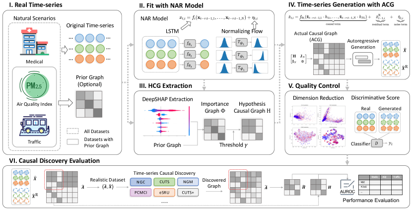
Figure 1: Illustration of our realistic time-series generation pipeline, which takes observations from real scenarios as input and produces benchmark data for performance evaluation of TSCD algorithms. The whole pipeline consists of several key steps, which are explained in Section 3 in detail.

3.1 Causal Model

Causal models in time-series are frequently represented as graphical models [56; 50]. However, different from the classic Pearl’s causality [37], spatio-temporal structural dependency must be taken into account for time-series data. We denote a uniformly sampled observation of a dynamic system as ${\bm{X}}=\{{\bm{x}}_{1:T,i}\}_{i=1}^{N}$, in which ${\bm{x}}_{t}$ is the sample vector at time point $t$ and consists of $N$ variables $\{x_{t,i}\}$, with $t\in\left\{1,...,T\right\}$ and $i\in\left\{1,...,N\right\}$. The structural causal model (SCM) for time-series [43] is $x_{t,i}=f_{i}\left(\mathcal{P}(x_{t,i}),\eta_{t,i}\right),~{}~{}~{}i=1,2,...,N$, where $f_{i}$ is any (potentially) nonlinear function, $\eta_{t,i}$ denotes dynamic noise with mutual independence, and $\mathcal{P}(x_{t}^{j})$ denotes the causal parents of $x_{t}^{j}$. This model is generalizable to most scenarios, but may bring obstacles for our implementation. In this paper, we consider the nonlinear autoregressive model (NAR), a slightly restricted class of SCM.

Nonlinear Autoregressive Model. We adopt the representation in many time-series causal discovery algorithms ([53; 31; 9]), as well as Lawrence et al. [28]’s time-series generation pipeline. In a Nonlinear Autoregressive Model (NAR), the noise is assumed to be independent and additive, and each sampled variable $x_{t,i}$ is generated by the following equation:

$$x_{t,i}=f_{i}\left(\mathcal{P}(x_{t,i})\right)+\eta_{t,i},~{}~{}~{}i=1,2,...,N.$$ (1)

where $\mathcal{P}(\cdot)$ denotes parents in causal graph. We further assume that the maximal time lags for causal effects are limited. Then the model can be denoted as $x_{t,i}=f_{i}\left(\{x_{\tau,j}\}_{x_{\tau,j}\in\mathcal{P}(x_{t,i})}\right)+\eta_{t,i}$. Here $t-\tau\leq\tau_{\text{max}},\forall x_{\tau,j}\in\mathcal{P}(x_{t,i})$, and $\tau_{\text{max}}$ denotes the maximal time lag. In causal discovery, time-homogeneity [17] is often assumed, i.e., function $f_{i}$ and causal parents $\mathcal{P}$ is irrelevant to time. By summarizing temporal dependencies, the summary graph for causal models can be denoted with binary matrix $\mathbf{A}$, where its element $a_{ji}=\begin{cases}1,&\exists\tau,s.t.,x_{\tau,j}\in\mathcal{P}(x_{t,i})\\ 0,&\text{otherwise}\end{cases}$. The dataset pair for causal discovery is $\left<\mathbf{X},\mathbf{A}\right>$. TSCD targets to recover matrix $\mathbf{{A}}$ given time-series $\mathbf{X}$. However, since for most real time-series $\mathbf{X}$, causal graph $\mathbf{A}$ is unknown, benchmarking causal discovery algorithms with real time-series is generally inappropriate.

3.2 Time-series Fitting

After collecting real-time-series from diverse fields, we fit the dynamic process of multivariate time-series with a deep neural network and normalizing flow.

Time-series Fitting with Causally Disentangled Neural Network (CDNN).     To fit the observed time-series with a deep neural network and introduce casual graphs into the network’s prediction of output series, Tank et al. [53]; Khanna & Tan [25]; Cheng et al. [9] separate the causal effects from the parents to each of individual output series using $N$ separate MLPs / LSTMs, which is referred to as component-wise MLP / LSTM (cMLP / cLSTM). In this paper, we follow [8]’s definition and refer to the component-wise neural networks as “causally disentangled neural networks”.

Definition 1

Let $\mathbf{X}\in\mathbf{\mathcal{X}}\subset\mathbb{R}^{T\times N},\mathbf{A}\in\mathbf{\mathcal{A}}\subset\left\{0,1\right\}^{n\times n}$ and $\mathbf{y}\in\mathbf{\mathcal{Y}}\subset\mathbb{R}^{n}$ be the input and output spaces. We say a neural network $\mathbf{f}_{\Theta}:\left<\mathbf{\mathcal{X}},\mathbf{\mathcal{A}}\right>\rightarrow\mathbf{\mathcal{Y}}$ is a causally disentangled neural network (CDNN) if it has the form

$$\mathbf{f}_{\Theta}(\mathbf{X},\mathbf{A})=\left[f_{\Theta_{1}}(\mathbf{X}\odot\mathbf{a}_{:,1}),...,f_{\Theta_{n}}(\mathbf{X}\odot\mathbf{a}_{:,n})\right]^{T},$$ (2)

where $\mathbf{a}_{:,j}$ is the column vector of input causal adjacency matrix $\mathbf{A}$; $f_{\phi_{j}}:\mathbf{\mathcal{X}}_{j}\rightarrow\mathbf{\mathcal{Y}}_{j}$, with $\mathbf{\mathcal{X}}_{j}\subset\mathbb{R}^{n}$ and $\mathbf{\mathcal{Y}}_{j}\subset\mathbb{R}$; the operator $\odot$ is defined as $f_{\phi_{j}}(\mathbf{X}\odot\mathbf{a}_{:,j})\overset{\Delta}{=}f_{\phi_{j}}\left(\left\{\mathbf{x}_{1}\cdot a_{1j},...,\mathbf{x}_{N}\cdot a_{Nj}\right\}\right)$.

So far function $f_{\Theta_{j}}(\cdot)$ acts as the neural network function used to approximate $f_{j}(\cdot)$ in Equation (1). Since we assume no prior on the underlying causal relationships, to extract the dynamics of the time-series with high accuracy, we fit the generation process with all historical variables (with maximal time lag $\tau_{\text{max}}$, which is discussed in Supplementary Section A.1.1) and obtain a fully connected graph. Specifically, we assume that

$$x_{t,i}=f_{i}\left(\mathbf{x}_{t-\tau:t-1,1},...,\mathbf{x}_{t-\tau:t-1,N}\right)+\eta_{t,i},~{}~{}~{}i=1,2,...,N.$$ (3)

In the following, we omit the time dimension of $\mathbf{x}_{t-\tau:t-1,j}$ and denote it with $\mathbf{x}_{j}$. Using a CDNN in Definition 1, we can approximate $f_{i}(\cdot)$ with $f_{\Theta_{i}}(\cdot)$. [53] and [9] implement CDNN with component-wise MLP / LSTM (cMLP / cLSTM), but the structure is highly redundant because it consists of $N$ distinct neural networks.

Implementation of CDNN.     The implementation of CDNN can vary. For example, Cheng et al. [8] explores enhancing causal discovery with a message-passing-based neural network, which is a special version of CDNN with extensive weight sharing. In this work, we utilize an LSTM-based CDNN with a shared decoder (with implementation details shown in Supplementary Section A.2). Moreover, we perform scheduled sampling [3] to alleviate the accumulated error when performing autoregressive generation.

Noise Distribution Fitting by Normalizing Flow.     After approximating the functional term $f_{i}(\cdot)$ with $f_{\Theta_{i}}(\cdot)$, we then approximate noise term $\eta_{t,i}$ with Normalizing Flow (NF) [26; 36]. The main process is described as

$$\hat{\eta}_{t,i}=T_{\psi_{i}}(u),\text{ where }u\sim p_{u}(u),$$ (4)

in which $T_{\psi_{i}}(\cdot)$ is an invertible and differentiable transformation implemented with neural network, $p_{u}(u)$ is the base distribution (normal distribution in our pipeline), and $p_{\hat{\eta}_{i}}(\hat{\eta}_{t,i})=p_{u}(T^{-1}_{\psi_{i}}(\hat{\eta}_{t,i}))\frac{\partial}{\partial\hat{\eta}_{t,i}}T^{-1}_{\psi_{i}}(\hat{\eta}_{t,i})$. Then, the optimization problem can be formulated as $\max_{\psi_{i}}\sum_{t=1}^{N}\log p_{u}(T^{-1}_{\psi_{i}}(\eta_{t,i}))+\log\frac{\partial}{\partial\eta_{t,i}}T^{-1}_{\psi_{i}}(\eta_{t,i})$

3.3 Extraction of Hypothetical Causal Graph

In the fully connected graph, all $N$ variables contribute to each prediction, which fits the observations quite well but is over-complicated than the latent causal graph. We now proceed to extract a hypothetical causal graph (HCG) $\mathbf{H}$ by identifying the most contributing variables in the prediction model $f_{\Theta_{i}}(\cdot)$. We would like to clarify that, extracting HCG is not causal discovery, and it instead targets to identify the contributing causal parents while preserving the fidelity of the fitting model. Two options are included in our pipeline: i) HCG extraction with DeepSHAP; ii) HCG extraction with prior knowledge.

HCG Extraction with DeepSHAP.     Shapley values [52] are frequently used to assign feature importance for regression models. It originates from cooperative game theory [27], and has recently been developed to interpret deep learning models (DeepSHAP) [32; 7]. For each prediction model $f_{\Theta_{i}}(\cdot)$, the calculated importance of each input time-series $\mathbf{x}_{t-\tau:t-1,j}$ by DeepSHAP is $\phi_{ji}$. By assigning importance values from each time-series $j$ to $i$, we get the importance matrix $\Phi$. After we set the sparsity $\sigma$ of a HCG, a threshold $\gamma$ can be calculated with cumulative distribution, i.e., $\gamma=F_{\phi}^{-1}(\sigma)$, where $F_{\phi}(\cdot)$ is the cumulative distribution of $\phi_{ji}$ if we assume all $\phi_{ji}$ are i.i.d.

HCG Extraction with Prior Knowledge.     Time-series in some fields, e.g., weather or traffic, relationships between each variable are highly relevant to geometry distances. For example, air quality or traffic flows in a certain area can largely affect that in a nearby area. As a result, geometry graphs can serve as hypothetical causal graphs (HCGs) in these fields, we show the HCG calculation process in Supplementary Section A.2 for this case.

The extracted HCGs is not the ground truth causal graph of time-series $\mathbf{X}$, because time-series $\mathbf{X}$ is not generated by the corresponding NAR or SCM model. A trivial solution would be running auto-regressive generation of time-series by setting input of non-causal terms to zero, i.e.,

$$\hat{x}_{t,i}=f_{\Theta_{i}}\left(\mathbf{\hat{x}}_{t-\tau:t-1,1}\cdot h_{1i},...,\mathbf{\hat{x}}_{t-\tau:t-1,N}\cdot h_{Ni}\right)+\hat{\eta}_{t,i},~{}~{}~{}i=1,2,...,N.$$ (5)

with $\{h_{ji}\}$ being the entries in the HCG $\mathbf{H}$. The fidelity of the fitting model $f_{\Theta_{i}}(\cdot)$ in Eq. 5 is greatly hampered by only including a subset of the variables. In the following, we introduce another way to generate a time-series with an actual causal graph, and most importantly, without losing fidelity.

3.4 Time-series Generation from the Actual Causal Graph

To acquire the Actual Causal Graphs (ACGs) with high data fidelity, we propose to split the NAR model taking the form of a fully connected graph into causal term, residual term, and noise term, i.e.,

$$\hat{x}_{t,i}=\underbrace{f_{\Theta_{i}}\left(\mathbf{\hat{x}}_{t-\tau:t-1,1}\cdot h_{1i},...,\mathbf{\hat{x}}_{t-\tau:t-1,N}\cdot h_{Ni}\right)}_{\text{causal term}}+\underbrace{\hat{x}^{\text{R}}_{t-1,i}}_{\text{residual term}}+\underbrace{\hat{\eta}_{t,i}}_{\text{noise term}},$$ (6)

Where the residual term $\hat{x}^{\text{R}}_{t-1,i}$ indicates the “causal effect” of non-parent time-series of time-series $i$ in HCG $\mathbf{H}$. In other words, causal terms represent the “major parts” of causal effects, and the residual term represents the remaining parts. Mathematically, $\hat{x}^{\text{R}}_{t-1,i}$ is calculated as

$$\hat{x}^{\text{R}}_{t-1,i}=f_{\Theta_{i}}\left(\mathbf{\hat{x}}_{t-\tau:t-1,1},...,\mathbf{\hat{x}}_{t-\tau:t-1,N}\right)-f_{\Theta_{i}}\left(\mathbf{\hat{x}}_{t-\tau:t-1,1}\cdot h_{1i},...,\mathbf{\hat{x}}_{t-\tau:t-1,N}\cdot h_{Ni}\right).$$ (7)

When treated as a generation model, $\mathbf{x}_{j}\rightarrow\mathbf{x}_{i}^{\text{R}}$ contains instantaneous effects, however, which does not affect the causal discovery result of $\mathbf{x}_{j}\rightarrow\mathbf{x}_{i}$ for most existing TSCD approaches, as we discussed in Supplementary Section A.1.2. After randomly selecting an initial sequence $\mathbf{X}_{t_{0}-\tau_{\text{max}}:t_{0}-1}$ from the original time-series $\mathbf{X}$, $\mathbf{x}_{i}$ and $\mathbf{x}_{i}^{\text{R}}$ is generated via the auto-regressive model, i.e., the prediction results from the previous time step are used for generating the following time step. Our final generated time-series include all $\mathbf{x}_{i}$ and $\mathbf{x}_{i}^{\text{R}}$, i.e., a total of $2N$ time-series are generated, and the ACG $\mathbf{\hat{A}}$ is of size $2N\times 2N$:

$$\mathbf{\hat{X}}=\left\{\mathbf{\hat{X}}_{t_{0}:t_{0}+T};\mathbf{\hat{X}}^{\text{R}}_{t_{0}:t_{0}+T}\right\},\ \ \mathbf{\hat{A}}=\left[\begin{array}[]{c c}\mathbf{{H}}&\mathbf{J}_{N}\\ \mathbf{I}_{N}&\mathbf{0}\end{array}\right]_{2N\times 2N}$$ (8)

where $\mathbf{J}_{N}$ is an all-one matrix, $T$ is the total length of the generated time-series. With the prediction model $f_{\theta_{i}}$, normalizing flow model $T_{\psi_{i}}$, and ACG $\mathbf{A}$, we can obtain the final dataset $\left<\mathbf{\hat{X}},\mathbf{\hat{A}}\right>$. $\mathbf{\hat{X}}$ is then feeded to TSCD algorithms to recover matrix $\mathbf{{A}}$ given time-series $\mathbf{\hat{X}}$.

4 Experiments

In this section, we demonstrate the CausalTime dataset built with the proposed pipeline, visualize and quantify the fidelity of the generated time-series, and then benchmark the performance of existing TSCD algorithms on CausalTime.

4.1 Statistics of the Benchmark Datasets

Theoretically, the proposed pipeline is generalizable to diverse fields. Here we generate 3 types of benchmark time-series from weather, traffic, and healthcare scenarios respectively, as illustrated in Fig. 2. As for the time-series of weather and traffic, relationships between two variables are highly relevant to their geometric distances, i.e., there exists a prior graph, while there is no such prior in the healthcare series. The detailed descriptions of three benchmark subsets are as follows:

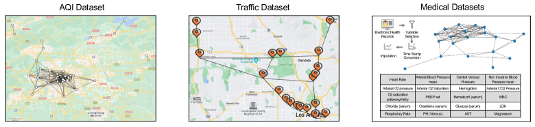
Figure 2: Visualization of three subsets in CausalTime. For AQI and Traffic, we overlay the ground truth causal graphs onto the map.

1. Air Quality Index (AQI) is a subset of several air quality features from 36 monitoring stations spread across Chinese cities, with an hourly measurement over one year. We consider the PM2.5 pollution index in the dataset. The total length of the dataset is L = 8760 and the number of nodes is N = 36. We acquire the prior graph by computing the pairwise distances between sensors (Supplementary Section A.2).

2. Traffic subset is built from the time-series collected by traffic sensors in the San Francisco Bay Area. The total length of the dataset is L = 52116 and we include 20 nodes, i.e., $N=20$. The prior graph is also calculated with the geographical distance (Supplementary Section A.2).

3. Medical subset is from MIMIC-4, which is a database that provides critical care data for over 40,000 patients admitted to intensive care units [22]. We select 20 most frequently tested vital signs and “chartevents” from 1000 patients, which are then transformed into time-series where each time point represents a 2-hour interval. The missing entries are imputed using the nearest interpolation. For this dataset, a prior graph is unavailable because of the extremely complex dynamics.

4.2 fidelity of the Generated Time-series

To qualitatively and quantitatively analyze the fidelity of the generated time-series, we utilize PCA Bryant & Yarnold [6] and t-SNE van der Maaten & Hinton [55] dimension reduction visualization, neural-network-based discriminative score, and MMD score of real and synthetic feature vectors to evaluate whether our generated time-series is realistic.

Visualization via Dimension Reduction.     To judge the fidelity of the generated time-series, we project the time-series features to a two-dimensional space, and assess their similarity by comparing the dimension reduction results. After splitting the original and generated time-series into short sequences (length of 5), we perform dimension reduction via linear (PCA) and nonlinear (t-SNE) approaches on three generated datasets and visualize the difference explicitly, as shown in Figure 3. One can observe that the distributions of the original and generated series are highly overlapped, and the similarity is especially prominent for AQI and Traffic datasets (i.e., the 1st, 2nd, 4th, and 5th columns). These results visually validate that our generated datasets are indeed realistic across a variety of fields.

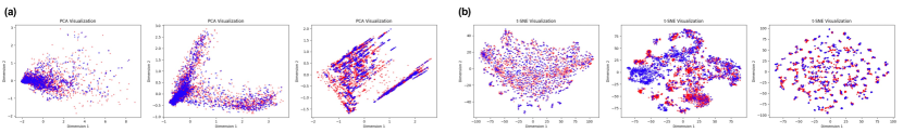
Figure 3: Visualization of the similarity between generated and original time-series in a low dimensional (2D) space, where original and generated series are shown in blue and red, respectively. (a) and (b) plots the two components of PCA and t-SNE on three datasets.

Discriminative Score / MMD Score. Other than visualization in low dimensional space, we further assess the generation quality, i.e., evaluate the similarity between the original and generated time-series, quantitatively using a neural-network-based discriminator and the MMD score. For the neural-network-based discriminator, by labeling the original time-series as positive samples and the generated time-series as negative ones, we train an LSTM classifier and then report the discriminative score in terms of $|\text{AUROC}-0.5|$ on the test set. MMD is a frequently used metric to evaluate the similarity of two distributions [19]. It is estimated with $\widehat{\mathrm{MMD}}^{2}_{u}=\frac{1}{n(n-1)}\sum_{i=1}^{n}\sum_{j\neq i}^{n}K(x_{i},x_{j})-\frac{2}{mn}\sum_{i=1}^{n}\sum_{j=1}^{m}K(x_{i},y_{j})+\frac{1}{m(m-1)}\sum_{i=1}^{m}\sum_{j\neq i}^{m}K(y_{i},y_{j})$, where $K$ is the radial basis function (RBF) kernel. MMD gives another quantitative evaluation of the similarity without the need to train another neural network, as listed in the bottom row of Table 2. It is observed that the generated dataset is similar to the original ones, since the discriminative score is very close to zero (i.e., neural networks cannot distinguish generated samples from original samples), and the MMD score is relatively low. Other than discriminative score and MMD, we also utilize cross-correlation scores and perform additive experiments, which is shown in Supplementary Section A.3.

Table 2: Quantitative assessment of the similarity between the generated and original time-series in terms of discriminative score and MMD. We show the ablation study in the table as well.

Datasets	Discriminative Score			MMD
	AQI	Traffic	Medical	AQI	Traffic	Medical
Additive Gaussian Noise	0.488 $\pm$ 0.001	0.499 $\pm$ 0.000	0.445 $\pm$ 0.003	0.533 $\pm$ 0.091	0.716 $\pm$ 0.011	0.480 $\pm$ 0.057
w/o Noise Term	0.361 $\pm$ 0.008	0.391 $\pm$ 0.006	0.346 $\pm$ 0.001	0.454 $\pm$ 0.025	0.717 $\pm$ 0.007	0.453 $\pm$ 0.029
Fit w/o Residual Term	0.309 $\pm$ 0.010	0.500 $\pm$ 0.000	0.482 $\pm$ 0.005	0.474 $\pm$ 0.033	0.858 $\pm$ 0.020	0.520 $\pm$ 0.023
Generate w/o Residual Term	0.361 $\pm$ 0.014	0.371 $\pm$ 0.003	0.348 $\pm$ 0.014	0.431 $\pm$ 0.055	0.657 $\pm$ 0.016	0.489 $\pm$ 0.037
Full Model	0.054 $\pm$ 0.025	0.039 $\pm$ 0.020	0.017 $\pm$ 0.027	0.246 $\pm$ 0.029	0.215 $\pm$ 0.013	0.461 $\pm$ 0.033

Ablation Study.     Using the above two quantitative scores, we also perform ablation studies to justify the effectiveness of our design. In the time-series fitting, we use normalizing flow to fit the noise distributions. To validate its effectiveness, we replace normalizing flow with (a) additive Gaussian noise (with parameters estimated from real series) and (b) no noise. Further, to validate that our pipeline reserves the real dynamics by splitting the causal model into causal term, residual term, and noise term, we add two alternatives that do not include the residual term when (c) fitting the NAR model or (d) generating new data, besides the above two settings.

The results are shown in Table 2, which shows that the full model produces time-series that mimic the original time-series best, in terms of both discriminative score and MMD score. The only exception is the slightly lower MMD under settings “w/o Noise” on medical datasets. It is worth noting that our discrimination scores are close to zero, i.e., neural networks cannot discriminate almost all generated time-series from original versions.

4.3 Performance of State-of-the-art Causal Discovery Algorithms

To quantify the performances of different causal discovery algorithms, here we calculate their AUROC and AUPRC with respect to the ground truth causal graph. We do not evaluate the accuracy of the discovered causal graph $\mathbf{\tilde{A}}$ with respect to its ground-truth $\mathbf{\hat{A}}$, because there exists instantaneous effects in $\mathbf{x}_{j}\rightarrow\mathbf{x}_{i}^{\text{R}}$ (see Supplementary Section A.1.2). Instead, we ignore the blocks $\mathbf{I}_{N},\mathbf{J}_{N}$ and $\mathbf{0}$ in Equation 8), and compare $\mathbf{\tilde{H}}$ with respect to $\mathbf{{H}}$,

Baseline TSCD Algorithms.     We benchmarked the performance of 9 most recent and representative causal discovery methods on our CausalTime datasets, including: Neural Granger Causality (NGC, [53]); economy-SRU (eSRU, [25]), a variant of SRU that is less prone to over-fitting when inferring Granger causality; Scalable Causal Graph Learning (SCGL, [59]) that addresses scalable causal discovery problem with low-rank assumption; Temporal Causal Discovery Framework (TCDF, [34]) that utilizes attention-based convolutional neural networks; CUTS [9] discovering causal relationships using two mutually boosting models, and CUTS+ [8] upgrading CUTS to high dimensional time-series. constraint-based approach PCMCI [43]; Latent Convergent Cross Mapping (LCCM, [5]); Neural Graphical Model (NGM, [2]), which employs neural ordinary differential equations to handle irregular time-series data. To ensure fairness, we searched for the best set of hyperparameters for these baseline algorithms on the validation dataset, and tested performances on testing sets for 5 random seeds per experiment.

Table 3: Performance benchmarking of baseline TSCD algorithms on our CausalTime datasets. We highlight the best and the second best in bold and with underlining, respectively.

Methods	AUROC			AUPRC
	AQI	Traffic	Medical	AQI	Traffic	Medical
CUTS	0.6013 $\pm$ 0.0038	0.6238 $\pm$ 0.0179	0.3739 $\pm$ 0.0297	0.5096 $\pm$ 0.0362	0.1525 $\pm$ 0.0226	0.1537 $\pm$ 0.0039
CUTS+	0.8928 $\pm$ 0.0213	0.6175 $\pm$ 0.0752	0.8202 $\pm$ 0.0173	0.7983 $\pm$ 0.0875	0.6367 $\pm$ 0.1197	0.5481 $\pm$ 0.1349
PCMCI	0.5272 $\pm$ 0.0744	0.5422 $\pm$ 0.0737	0.6991 $\pm$ 0.0111	0.6734 $\pm$ 0.0372	0.3474 $\pm$ 0.0581	0.5082 $\pm$ 0.0177
NGC	0.7172 $\pm$ 0.0076	0.6032 $\pm$ 0.0056	0.5744 $\pm$ 0.0096	0.7177 $\pm$ 0.0069	0.3583 $\pm$ 0.0495	0.4637 $\pm$ 0.0121
NGM	0.6728 $\pm$ 0.0164	0.4660 $\pm$ 0.0144	0.5551 $\pm$ 0.0154	0.4786 $\pm$ 0.0196	0.2826 $\pm$ 0.0098	0.4697 $\pm$ 0.0166
LCCM	0.8565 $\pm$ 0.0653	0.5545 $\pm$ 0.0254	0.8013 $\pm$ 0.0218	0.9260 $\pm$ 0.0246	0.5907 $\pm$ 0.0475	0.7554 $\pm$ 0.0235
eSRU	0.8229 $\pm$ 0.0317	0.5987 $\pm$ 0.0192	0.7559 $\pm$ 0.0365	0.7223 $\pm$ 0.0317	0.4886 $\pm$ 0.0338	0.7352 $\pm$ 0.0600
SCGL	0.4915 $\pm$ 0.0476	0.5927 $\pm$ 0.0553	0.5019 $\pm$ 0.0224	0.3584 $\pm$ 0.0281	0.4544 $\pm$ 0.0315	0.4833 $\pm$ 0.0185
TCDF	0.4148 $\pm$ 0.0207	0.5029 $\pm$ 0.0041	0.6329 $\pm$ 0.0384	0.6527 $\pm$ 0.0087	0.3637 $\pm$ 0.0048	0.5544 $\pm$ 0.0313

Results and Analysis.     From the scores in Table 3, one can see that among these algorithms, CUTS+ and LCCM perform the best, and most of the TSCD algorithms do not get AUROC $>0.9$. Interestingly, a few results demonstrate AUROC $<0.5$, which means that we get inverted classifications. The low accuracies tell that current TSCD algorithms still have a long way to go before being put into practice and indicate the necessity of designing more advanced algorithms with high feasibility to real data. Besides, compared with the reported results in previous work , one can notice that the scores on our CausalTime dataset are significantly lower than those on synthetic datasets (e.g., VAR and Lorenz-96), on which some TSCD algorithms achieve scores close to 1. This implies that the existing synthetic datasets are insufficient to evaluate the algorithm performance on real data and calls for building new benchmarks to advance the development in this field.

5 Additional Information

We place theoretical analysis and assumptions in Supplementary Section A.1, implementation details along with hyperparameters for each of our key steps in Section A.2, additional experimental results (including a comparison of various CDNN implementations, ablation study for scheduled sampling, and experimental results for cross-correlation scores) in Section A.3, and algorithmic representation for our pipeline in Section 1.

6 Conclusions

We propose CausalTime, a novel pipeline to generate realistic time-series with ground truth causal graphs, which can be used to assess the performance of TSCD algorithms in real scenarios and can also be generalizable to diverse fields. Our CausalTime contributes to the causal-discovery community by enabling upgraded algorithm evaluation under diverse realistic settings, which would advance both the design and applications of TSCD algorithms. Our code is available at https://github.com/jarrycyx/unn.

Our work can be further developed in multiple aspects. Firstly, replacing NAR with the SCM model can extend CausalTime to a richer set of causal models; secondly, we plan to take into account the multi-scale causal effects that widely exist in realistic time-series. Our future works include i) Creating a more realistic time-series by incorporating prior knowledge of certain dynamic processes or multi-scale associations. ii) Investigation of an augmented TSCD algorithm with reliable results on real time-series data.

Appendix A Appendix

A.1 Theory

A.1.1 Assumptions

Several assumptions are needed for our causal models, which are common in causal discovery literature.

Markovian Condition. The joint distribution can be factorized into $P(\mathbf{x})=\prod_{i}P(x_{i}|\mathcal{P}(x_{i}))$, i.e., every variable is independent of all its nondescendants, conditional on its parents.

Causal Faithfulness. A causal model that accurately reflects the independence relations present in the data.

Causal Sufficiency. (or no latent confounder) All common causes of all variables are observed. This assumption is potentially very strong since we cannot observe “all causes in the world” because it may include infinite variables. However, this assumption is important for a variety of literature.

No Instantaneous Effect. (Or Temporal Priority [1]) The cause occurred before its effect in the time-series. This assumption can be satisfied if the sampling frequency is higher than the causal effects. However, this assumption may be strong because the sampling frequency of many real time-series is not high enough.

Causal Stationarity. All the causal relationships remain constant throughout time. With this assumption, full time causal graph can be summarized into a windowed causal graph [1].

Other than these assumptions, we explicitly define a maximum time lag $\tau_{\text{max}}$ for causal effects (Section 3.2). However, long-term or multi-scale associations are common in many time-series [12; 58]. We make this restriction because most causal discovery algorithm does not consider long-term or multi-scale associations.

A.1.2 Instantaneous Effect of Residual Term

In section 3.4, we propose to split the NAR model into causal term, residual term, and noise term, where the residual term $x_{t-1}^{\text{R}}$ is generated with

$$\hat{x}^{\text{R}}_{t-1,i}=f_{\Theta_{i}}\left(\mathbf{\hat{x}}_{t-\tau:t-1,1},...,\mathbf{\hat{x}}_{t-\tau:t-1,N}\right)-f_{\Theta_{i}}\left(\mathbf{\hat{x}}_{t-\tau:t-1,1}\cdot h_{1i},...,\mathbf{\hat{x}}_{t-\tau:t-1,N}\cdot h_{Ni}\right)$$ (9)

As a result, instantaneous effects exist in this generation equation, i.e., in $\mathbf{x}_{j}\rightarrow\mathbf{x}_{i}^{\text{R}}$ but not in $\mathbf{x}_{j}\rightarrow\mathbf{x}_{i}$, $\forall i,j$. This is not a problem when tested on TSCD algorithms with compatibility with instantaneous effects. In the following, we discuss the consequences when tested on TSCD algorithms without compatibility to instantaneous effects, e.g., Granger Causality, Convergent Cross Mapping, and PCMCI [45]. For most cases, this does not affect causal discovery results between all $\mathbf{x}_{j}$. Though they may draw a wrong conclusion of $\mathbf{x}_{j}\nrightarrow\mathbf{x}_{i}^{\text{R}}$, this is not the part we compare to ground truth in the evaluation (Section 4.3).

Granger Causality. Granger Causality determines causal relationships by testing if a time-series helps the prediction of another time-series. In this case, the causal discovery results of $\mathbf{x}_{j}\rightarrow\mathbf{x}_{i}$ are not affected since instantaneous effects of $\mathbf{x}_{j}\rightarrow\mathbf{x}_{i}^{\text{R}}$ do not affect whether the time-series $\mathbf{x}_{j}$ helps to predict the time-series $\mathbf{x}_{i}$, $\forall i,j$.

Constraint-based Causal Discovery. These line of works is based on conditional independence tests, i.e., if $\mathbf{x}_{t_{0},j}\rightarrow\mathbf{x}_{t,i}$, then ${x}_{t_{0},j}\not\!\perp\!\!\!\perp{x}_{t,i}|\mathbf{X}_{t-\tau:t-1}\backslash\{{x}_{t_{0},j}\}$, where $t-\tau\leq t_{0}<t$ [43; 41]. This relationship is unaffected when considering instantaneous effect of ${x}_{t,j}\rightarrow{x}_{t,i}^{\text{R}}$, since all paths from ${x}_{t_{0},j}$ to ${x}_{t,i}$ through ${x}_{t,k}^{\text{R}}$ are blocked by conditioning on ${x}_{t,k}^{\text{R}}$, $\forall i,j,k$, as is shown in Fig. 4.

CCM-based Causal Discovery. CCM detects if time-series $\mathbf{x}$ causes time-series $\mathbf{y}$ by examine whether time indices of nearby points on the $\mathbf{y}$ manifold can be used to identify nearby points on $\mathbf{x}$ [51; 5]. In this case, the examination of whether $\mathbf{x}_{j}\rightarrow\mathbf{x}_{i}$ is not affected by $\mathbf{x}_{k}^{\text{R}}$, $\forall i,j,k$.

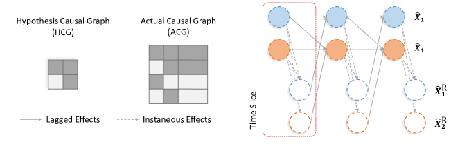
Figure 4: Illustration of instantaneous effects of $\mathbf{x}_{j}\rightarrow\mathbf{x}_{i}^{\text{R}}$. All paths from ${x}_{t_{0},j}$ to ${x}_{t,i}$ through ${x}_{t,k}^{\text{R}}$ are blocked by conditioning on ${x}_{t,k}^{\text{R}}$, $\forall i,j,k$.

A.2 Implementation Details

Network Structures and Training. The implementation of CDNN can vary and cMLP / cLSTM is not the only choice. For example, Cheng et al. [8] explores enhancing causal discovery with a message-passing-based neural network, which is a special version of CDNN with extensive weight sharing. However, the fitting accuracy of CDNN is less explored. Sharing partial weights may alleviate the structural redundancy problem. Moreover, the performance with more recent structures is unknown, e.g. Transformer. In the following, this work investigates various implementations of CDNN when they are applied to fit causal models.

Specifically, three kinds of backbones combining three network sharing policies are applied, i.e., MLP, LSTM, Transformer combining no sharing, shared encoder, and shared decoder. For MLP, the encoder and decoder are both MLP. For LSTM, we assign an LSTM encoder and an MLP decoder. For the Transformer, we assign a Transformer encoder and MLP decoder. We show the structure for no sharing, shared encoder, and shared decoder in Figure 5, with a three-variable example. The test results for prediction using these architectures are shown in Table 6.

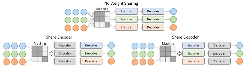
Figure 5: Illustration of network structures of CDNN.

Table 4: Hyper parameters for time-series fitting.

Module	Parameter	AQI	Traffic	Medical
LSTM Encoder	Layers	2	2	2
	Hidden	128	128	128
	Heads	4	4	4
MLP Encoder	Layers	3	3	3
	Hidden	128	128	128
Transformer Encoder	Hidden	128	128	128
	Heads	4	4	4
Decoder	Layers	3	3	3
	Hidden	128	128	128
Training	Learning Rate	0.01	0.001	0.003
	Optimizer	Adam	Adam	Adam
	Input Window	20	20	20
Normalizing Flow	Layers	5	5	5
	Hidden	128	64	64

Table 5: Hyperparameters settings of the baseline causal discovery and data imputation algorithms.

Methods	Params.	AQI	Traffic	Medical
PCMCI	$\tau_{max}$	5	5	5
	$PC_{\alpha}$	0.05	0.05	0.05
NGC	Learning rate	0.05	0.05	0.05
	$\lambda_{ridge}$	0.01	0.01	0.01
	$\lambda$	$0.02\rightarrow 0.2$	$0.02\rightarrow 0.2$	$0.02\rightarrow 0.2$
eSRU	$\mu_{1}$	0.1	0.1	0.7
	Learning rate	0.01	0.01	0.001
	Batch size	40	40	40
	Epochs	50	50	50
SCGL	$\tau$	10	10	10
	Batch size	32	32	32
	Window	3	3	3
LCCM	Epochs	50	50	50
	Batch size	10	10	10
	Hidden size	20	20	20
NGM	Steps	200	200	200
	Horizon	5	5	5
	GL_reg	0.05	0.05	0.05
TCDF	$\tau$	10	10	10
	Epoch num	1000	1000	1000
	Learning rate	0.01	0.01	0.01
CUTS	Input step	20	20	20
	$\lambda$	0.1	0.1	0.1
	$\tau$	$0.1\rightarrow 1$	$0.1\rightarrow 1$	$0.1\rightarrow 1$
CUTS+	Input step	1	1	1
	$\lambda$	0.01	0.01	0.01
	$\tau$	$0.1\rightarrow 1$	$0.1\rightarrow 1$	$0.1\rightarrow 1$

Normalizing Flow. We implement normalizing flow using its open-source repository. We use normal distributions as base distributions. For transformations, we use simple combinations of linear and nonlinear layers, with parameters shown in Table 4.

DeepSHAP. We use the official implementation of DeepSHAP. Specifically, we use its “DeepExplainer” module to explain the time-series prediction model which is trained with a fully connected graph. Note that this prediction model is a CDNN, which enables a pairwise explanation of feature $i$’s importance to the prediction of $j$. The explained samples are randomly selected from a train set of real time-series, and the final feature importance graph $\Phi$ is acquired by taking the average values of all samples. To convert to binarized HCG, we select a threshold to get a sparsity of 15% (i.e., 15% of the elements in HCG are labeled as 1).

Prior Graph Extraction. For datasets with prior knowledge, e.g., AQI and Traffic, relationships between each variable are highly relevant to geometry distances. Consequently, we extract HCG from the geographic distances between nodes using a thresholded Gaussian kernel, i.e.,

$$w^{ij}=\begin{cases}1,&\text{dist}(i,j)\leq\sigma\\ 0,&\text{otherwise}\end{cases}$$ (10)

we select $\sigma$ based on geographical distances (which is $\approx 40$ km for AQI dataset and for Traffic dataset, we use the “dist_graph” from https://github.com/liyaguang/DCRNN/tree/master).

Dimension Reduction. For the implementation of t-SNE and PCA, we use scikit-learn package. To solve the dimension reduction in an acceptable time, we split the generated time-series into short sequences (with lengths of 5) and flattened them for the input of dimension reduction.

Autoregressive Generation. After fitting the time-series with neural networks and normalizing flow, and acquiring the ground-truth causal graph by splitting the causal model, we generate a new time-series autoregressively. Although we utilize scheduled sampling to avoid the accumulation of the generation error, the total time step must be limited to a relatively small one. Actually, our generated time length is 40 for these three datasets. For each of them, we generate 500 samples, i.e., a total of 20000 time steps for each dataset.

TSCD Algorithm Evaluation. Since our generated time-series are relatively short and contain several samples, we alter existing approaches by enabling TSCD from multiple observations (i.e. multiple time-series). For neural-network-based or optimization-based approaches such as CUTS, CUTS+, NGC, and TCDF, we alter their dataloader module to prevent cross-sample data fetching. For PCMCI, we use its variant JPCMCI+ which permits the input of multiple time-series. For remaining TSCD algorithms that do not support multiple time-series, we use zero-padding to isolate each sample. We list the original implementations of our included TSCD algorithms in the following:

• PCMCI.     The code is from https://github.com/jakobrunge/tigramite.

• NGC.     The code is from https://github.com/iancovert/Neural-GC. We use the cMLP network because according to the original paper [53] cMLP achieves better performance, except for Dream-3 dataset.

• eSRU.     The code is from https://github.com/sakhanna/SRU_for_GCI.

• SCGL.     The code is downloaded from the link shared in its original paper [59].

• LCCM.     The code is from https://github.com/edebrouwer/latentCCM.

• NGM.     The code is from https://github.com/alexisbellot/Graphical-modelling- continuous-time.

• CUTS / CUTS+.     The code is from https://github.com/jarrycyx/UNN.

• TCDF.     The code is from https://github.com/M-Nauta/TCDF.

Discriminative Network. To implement the discrimination score in time-series quality control, we train separate neural networks for each dataset to classify the original from the generated time-series. We use a 2-layered LSTM a with hidden size of 8, the training is performed with a learning rate of 1e-4 and a total of 30 epochs.

A.3 Additional Results

A.3.1 Time-series Fitting

In Section 3.2, we show that CDNN can be used to fit causal models with adjacency matrix $\mathbf{A}$. By splitting each network into two parts, i.e., encoder and decoder, 9 combinations (MLP, LSTM, Transformer combining shared encoder, shared decoder, and no weight sharing) are considered in the experiments. By comparing fitting accuracy (or prediction accuracy) on the AQI dataset, we observe that LSTM with a shared decoder performs the best among 9 implementations.

Table 6: Comparison of predictive MSE with different implementations of CDNN. The experiments are performed on AQI datasets.

Backbone		MLP	LSTM	Transformer
Weight Sharing	No Sharing	$0.0511\pm 0.0009$	$0.0017\pm 0.0002$	$.0061\pm 0002$
	Shared Encoder	$0.0248\pm 0.0033$	$0.0048\pm 0.0002$	$0.0056\pm 0.0001$
	Shared Decoder	$0.0254\pm 0.0024$	0.0014 $\pm$ 0.0002	$0.0060\pm 0.0002$

A.3.2 Scheduled Sampling

To validate if scheduled sampling is effective in the training process, we perform an ablation study on three datasets with different autoregressive prediction steps. We observe in Table 7 that, by incorporating scheduled sampling, the cumulative error decreases, and the decrement is large with higher autoregressive steps. This demonstrates that scheduled sampling does decrease accumulative error for the fitting model, which is beneficial for the following generation process.

Table 7: Comparison of prediction MSE with and without scheduled sampling policy. The comparisons are performed with different autoregressive prediction steps $n$ in terms of MSE.

Step	AQI		Traffic		Medical
	w	w/o	w	w/o	w	w/o
$n=2$	0.0129	0.0123	0.0124	0.0124	0.0082	0.0082
$n=5$	0.0348	0.0329	0.0279	0.0282	0.0136	0.0155
$n=10$	0.0351	0.0377	0.0312	0.0354	0.0181	0.0193
$n=20$	0.0331	0.034	0.0318	0.0331	0.0144	0.0174

A.3.3 Cross Correlation Scores for Time-series Generation

Despite the discriminative score and MMD score, we further compare the similarity of generated data to original versions in terms of cross-correlation scores. Specifically, we calculate the correlation between real and generated feature vectors, and then report the sum of the absolute differences between them, which is similar to Jarrett et al. [21]’s calculation process. We show the results along with the ablation study in Table 8.

Table 8: Quantitative assessment of the similarity between the generated and original time-series in terms of cross-correlation scores. We show the ablation study in the table as well.

Datasets	Cross Correlation Score
	AQI	Traffic	Medical
Additive Gaussian Noise	43.74 $\pm$ 11.55	198.30 $\pm$ 4.00	18.91 $\pm$ 2.17
w/o Noise Term	50.04 $\pm$ 4.79	194.44 $\pm$ 5.02	20.77 $\pm$ 4.40
Fit w/o Residual Term	49.04 $\pm$ 7.01	238.38 $\pm$ 4.90	21.94 $\pm$ 3.45
Generate w/o Residual Term	40.62 $\pm$ 24.73	164.14 $\pm$ 3.04	23.53 $\pm$ 3.12
Full Model	39.75 $\pm$ 5.24	60.37 $\pm$ 2.88	22.37 $\pm$ 1.59

A.4 Algorithmic Representation for CausalTime Pipeline

We show the detailed algorithmic representation of our proposed data generation pipeline in Algorithm 1, where we exclude quality control and TSCD evaluation steps.

Algorithm 1 Pipeline for CausalTime Generation (Excluding quality control and TSCD evaluation)

0:  Time-series dataset $\mathbf{X}=\left\{{\bm{x}}_{1:L,1},...,{\bm{x}}_{1:L,N}\right\}$ with length $L$; (Optional) graph $\mathbf{H}_{p}$ generated with prior knowledge; generation length $\hat{L}$.

0:  Paired time-series causal discovery (TSCD) dataset $\left<\mathbf{\hat{X}},\mathbf{\hat{A}}\right>$.

  Initilize parameter set $\{\Theta_{i}\}_{i=1}^{N}$, $\{\Psi_{i}\}_{i=1}^{N}$

  # Time-series Fitting

  for $n_{1}$ Epochs do

     Update $\{\Theta_{i}\}_{i=1}^{N}$ with Algorithm 2 (Prediction Model Fitting).

  end for

  for $n_{1}$ Epochs do

     Update $\{\Psi_{i}\}_{i=1}^{N}$ with Algorithm 3 (Noise Distribution Fitting).

  end for

  # HCG Extraction

  if Exists prior knowledge $\mathbf{H}_{p}$ then

     $\mathbf{H}\leftarrow\mathbf{H}_{p}$

  else

     $\mathbf{H}\leftarrow\left\{\text{DeepSHAP}\left({f_{\Theta_{i}}}(\cdot)\right)\right\}_{i=1}^{N}$

  end if

  $\mathbf{H}\leftarrow\mathbb{I}(\mathbf{H}>\gamma)$, where calculation of $\gamma$ is discussed in Section 5.

  # Time-series Generation with ACG

  Generate actual causal graph $\mathbf{\hat{A}}$ with Equation 8, select initial sequence $\mathbf{\hat{X}}_{0:\tau-1}$ randomly from original time-series $\mathbf{X}$.

  for $t=\tau$ top $\hat{L}$ do

     for $i=1$ top $N$ do

        Generate $\hat{x}_{t,i}$ and $\hat{x}_{t,i}^{\text{R}}$ with Equation 6 and 7, where $\hat{\eta}_{t,i}$ is sampled from $T_{\Psi_{i}}(u)$.

     end for

  end for

  return  Generated TSCD dataset $\left<\mathbf{\hat{X}},\mathbf{\hat{A}}\right>$.

Algorithm 2 Prediction Model Fitting

0:  Time-series dataset $\left\{{\bm{x}}_{1:L,1},...,{\bm{x}}_{1:L,N}\right\}$ with length $L$; parameter set $\{\Theta_{i}\}_{i=1}^{N}$.

0:  Paired time-series causal discovery (TSCD) dataset $\left<\mathbf{\hat{X}},\mathbf{\hat{A}}\right>$.

  for $i=1$ top $N$ do

     Perform prediction with $\hat{x}_{t,i}\leftarrow f_{\Theta_{i}}\left(\mathbf{x}_{t-\tau:t-1,1},...,\mathbf{x}_{t-\tau:t-1,N}\right)+\eta_{t,i}$

     Calculate loss function with $\text{MSE}(\hat{X},{X})$

     Update $\{\Theta_{i}\}_{i=1}^{N}$ with Adam optimizer

  end for

  return  Discovered causal adjacency matrix $\hat{{\bm{A}}}$ where each elements is $\tilde{a}_{i,j}$.

Algorithm 3 Noise Distribution Fitting

0:  Time-series dataset $\left\{{\bm{x}}_{1:L,1},...,{\bm{x}}_{1:L,N}\right\}$ with length $L$; Parameter set $\{\Theta_{i}\}_{i=1}^{N}$, $\{\Psi_{i}\}_{i=1}^{N}$.

0:  Paired time-series causal discovery (TSCD) dataset $\left<\mathbf{\hat{X}},\mathbf{\hat{A}}\right>$.

  for $i=1$ top $N$ do

     Perform prediction with $\hat{x}_{t,i}\leftarrow f_{\Theta_{i}}\left(\mathbf{x}_{t-\tau:t-1,1},...,\mathbf{x}_{t-\tau:t-1,N}\right)+\eta_{t,i}$.

     Calculate real noise $\eta_{t,i}\leftarrow x_{t,i}-\hat{x}_{t,i}$.

     Calculate likelihood $p_{\eta_{i}}(\eta_{t,i})\leftarrow p_{u}(T^{-1}_{\psi_{i}}(\eta_{t,i}))\frac{\partial}{\partial\eta_{t,i}}T^{-1}_{\psi_{i}}(\eta_{t,i})$.

     Update $\{\Psi_{i}\}_{i=1}^{N}$ with Adam optimizer.

  end for

  return  Discovered causal adjacency matrix $\hat{{\bm{A}}}$ where each elements is $\tilde{a}_{i,j}$.

References

- Assaad et al. [2022] Charles K. Assaad, Emilie Devijver, and Eric Gaussier. Survey and evaluation of causal discovery methods for time series. Journal of Artificial Intelligence Research, 73:767–819, February 2022. ISSN 1076-9757. doi: 10.1613/jair.1.13428.
- Bellot et al. [2022] Alexis Bellot, Kim Branson, and Mihaela van der Schaar. Neural graphical modelling in continuous-time: Consistency guarantees and algorithms. In International Conference on Learning Representations, February 2022.
- Bengio et al. [2015] Samy Bengio, Oriol Vinyals, Navdeep Jaitly, and Noam Shazeer. Scheduled Sampling for Sequence Prediction with Recurrent Neural Networks. In Advances in Neural Information Processing Systems, volume 28. Curran Associates, Inc., 2015.
- Benkő et al. [2020] Zsigmond Benkő, Ádám Zlatniczki, Marcell Stippinger, Dániel Fabó, András Sólyom, Loránd Erőss, András Telcs, and Zoltán Somogyvári. Complete Inference of Causal Relations between Dynamical Systems, February 2020.
- Brouwer et al. [2021] Edward De Brouwer, Adam Arany, Jaak Simm, and Yves Moreau. Latent Convergent Cross Mapping. In International Conference on Learning Representations, March 2021.
- Bryant & Yarnold [1995] Fred B. Bryant and Paul R. Yarnold. Principal-components analysis and exploratory and confirmatory factor analysis. In Reading and Understanding Multivariate Statistics, pp. 99–136. American Psychological Association, Washington, DC, US, 1995. ISBN 978-1-55798-273-5.
- Chen et al. [2022] Hugh Chen, Scott M. Lundberg, and Su-In Lee. Explaining a series of models by propagating Shapley values. Nature Communications, 13(1):4512, August 2022. ISSN 2041-1723. doi: 10.1038/s41467-022-31384-3.
- Cheng et al. [2023a] Yuxiao Cheng, Lianglong Li, Tingxiong Xiao, Zongren Li, Qin Zhong, Jinli Suo, and Kunlun He. CUTS+: High-dimensional Causal Discovery from Irregular Time-series, August 2023a.
- Cheng et al. [2023b] Yuxiao Cheng, Runzhao Yang, Tingxiong Xiao, Zongren Li, Jinli Suo, Kunlun He, and Qionghai Dai. CUTS: Neural Causal Discovery from Irregular Time-Series Data. In The Eleventh International Conference on Learning Representations, February 2023b.
- Chevalley et al. [2023a] Mathieu Chevalley, Yusuf Roohani, Arash Mehrjou, Jure Leskovec, and Patrick Schwab. CausalBench: A Large-scale Benchmark for Network Inference from Single-cell Perturbation Data, July 2023a.
- Chevalley et al. [2023b] Mathieu Chevalley, Jacob Sackett-Sanders, Yusuf Roohani, Pascal Notin, Artemy Bakulin, Dariusz Brzezinski, Kaiwen Deng, Yuanfang Guan, Justin Hong, Michael Ibrahim, Wojciech Kotlowski, Marcin Kowiel, Panagiotis Misiakos, Achille Nazaret, Markus Püschel, Chris Wendler, Arash Mehrjou, and Patrick Schwab. The CausalBench challenge: A machine learning contest for gene network inference from single-cell perturbation data, August 2023b.
- D’Acunto et al. [2022] Gabriele D’Acunto, Paolo Di Lorenzo, and Sergio Barbarossa. Multiscale causal structure learning, July 2022.
- Esteban et al. [2017] Cristóbal Esteban, Stephanie L. Hyland, and Gunnar Rätsch. Real-valued (Medical) Time Series Generation with Recurrent Conditional GANs, December 2017.
- Geffner et al. [2022] Tomas Geffner, Javier Antoran, Adam Foster, Wenbo Gong, Chao Ma, Emre Kiciman, Amit Sharma, Angus Lamb, Martin Kukla, Nick Pawlowski, Miltiadis Allamanis, and Cheng Zhang. Deep End-to-end Causal Inference, June 2022.
- Gerhardus & Runge [2020] Andreas Gerhardus and Jakob Runge. High-recall causal discovery for autocorrelated time series with latent confounders. In Advances in Neural Information Processing Systems, volume 33, pp. 12615–12625. Curran Associates, Inc., 2020.
- Göbler et al. [2023] Konstantin Göbler, Tobias Windisch, Tim Pychynski, Steffen Sonntag, Martin Roth, and Mathias Drton. $\texttt{causalAssembly}$: Generating Realistic Production Data for Benchmarking Causal Discovery, June 2023.
- Gong et al. [2023] Chang Gong, Di Yao, Chuzhe Zhang, Wenbin Li, and Jingping Bi. Causal Discovery from Temporal Data: An Overview and New Perspectives, March 2023.
- Granger [1969] C. W. J. Granger. Investigating causal relations by econometric models and cross-spectral methods. Econometrica, 37(3):424–438, 1969. ISSN 0012-9682. doi: 10.2307/1912791.
- Gretton et al. [2006] Arthur Gretton, Karsten Borgwardt, Malte Rasch, Bernhard Schölkopf, and Alex Smola. A Kernel Method for the Two-Sample-Problem. In Advances in Neural Information Processing Systems, volume 19. MIT Press, 2006.
- Hoyer et al. [2008] Patrik Hoyer, Dominik Janzing, Joris M Mooij, Jonas Peters, and Bernhard Schölkopf. Nonlinear causal discovery with additive noise models. In Advances in Neural Information Processing Systems, volume 21. Curran Associates, Inc., 2008.
- Jarrett et al. [2021] Daniel Jarrett, Ioana Bica, and Mihaela van der Schaar. Time-series Generation by Contrastive Imitation. In Advances in Neural Information Processing Systems, volume 34, pp. 28968–28982. Curran Associates, Inc., 2021.
- Johnson et al. [2023] Alistair E. W. Johnson, Lucas Bulgarelli, Lu Shen, Alvin Gayles, Ayad Shammout, Steven Horng, Tom J. Pollard, Sicheng Hao, Benjamin Moody, Brian Gow, Li-wei H. Lehman, Leo A. Celi, and Roger G. Mark. MIMIC-IV, a freely accessible electronic health record dataset. Scientific Data, 10(1):1, January 2023. ISSN 2052-4463. doi: 10.1038/s41597-022-01899-x.
- Kang et al. [2020] Yanfei Kang, Rob J. Hyndman, and Feng Li. GRATIS: GeneRAting TIme Series with diverse and controllable characteristics. Statistical Analysis and Data Mining: The ASA Data Science Journal, 13(4):354–376, 2020. ISSN 1932-1872. doi: 10.1002/sam.11461.
- Karimi & Paul [2010] A. Karimi and M. R. Paul. Extensive chaos in the lorenz-96 model. Chaos: An Interdisciplinary Journal of Nonlinear Science, 20(4):043105, December 2010. ISSN 1054-1500. doi: 10.1063/1.3496397.
- Khanna & Tan [2020] Saurabh Khanna and Vincent Y. F. Tan. Economy statistical recurrent units for inferring nonlinear granger causality. In International Conference on Learning Representations, March 2020.
- Kobyzev et al. [2021] Ivan Kobyzev, Simon J.D. Prince, and Marcus A. Brubaker. Normalizing Flows: An Introduction and Review of Current Methods. IEEE Transactions on Pattern Analysis and Machine Intelligence, 43(11):3964–3979, November 2021. ISSN 1939-3539. doi: 10.1109/TPAMI.2020.2992934.
- Kuhn & Tucker [2016] Harold William Kuhn and Albert William Tucker. Contributions to the Theory of Games (AM-28), Volume II. Princeton University Press, March 2016. ISBN 978-1-4008-8197-0.
- Lawrence et al. [2021] Andrew R. Lawrence, Marcus Kaiser, Rui Sampaio, and Maksim Sipos. Data Generating Process to Evaluate Causal Discovery Techniques for Time Series Data, April 2021.
- Li et al. [2020] Yunzhu Li, Antonio Torralba, Anima Anandkumar, Dieter Fox, and Animesh Garg. Causal discovery in physical systems from videos. In Advances in Neural Information Processing Systems, volume 33, pp. 9180–9192. Curran Associates, Inc., 2020.
- Lippe et al. [2021] Phillip Lippe, Taco Cohen, and Efstratios Gavves. Efficient neural causal discovery without acyclicity constraints. In International Conference on Learning Representations, September 2021.
- Löwe et al. [2022] Sindy Löwe, David Madras, Richard Zemel, and Max Welling. Amortized causal discovery: Learning to infer causal graphs from time-series data. In Proceedings of the First Conference on Causal Learning and Reasoning, pp. 509–525. PMLR, June 2022.
- Lundberg & Lee [2017] Scott M Lundberg and Su-In Lee. A unified approach to interpreting model predictions. In Advances in Neural Information Processing Systems, volume 30. Curran Associates, Inc., 2017.
- Mooij et al. [2011] Joris M Mooij, Dominik Janzing, Tom Heskes, and Bernhard Schölkopf. On Causal Discovery with Cyclic Additive Noise Models. In Advances in Neural Information Processing Systems, volume 24. Curran Associates, Inc., 2011.
- Nauta et al. [2019] Meike Nauta, Doina Bucur, and Christin Seifert. Causal discovery with attention-based convolutional neural networks. Machine Learning and Knowledge Extraction, 1(1):312–340, March 2019. ISSN 2504-4990. doi: 10.3390/make1010019.
- Pamfil et al. [2020] Roxana Pamfil, Nisara Sriwattanaworachai, Shaan Desai, Philip Pilgerstorfer, Konstantinos Georgatzis, Paul Beaumont, and Bryon Aragam. DYNOTEARS: Structure learning from time-series data. In Proceedings of the Twenty Third International Conference on Artificial Intelligence and Statistics, pp. 1595–1605. PMLR, June 2020.
- Papamakarios et al. [2021] George Papamakarios, Eric Nalisnick, Danilo Jimenez Rezende, Shakir Mohamed, and Balaji Lakshminarayanan. Normalizing flows for probabilistic modeling and inference. The Journal of Machine Learning Research, 22(1):57:2617–57:2680, January 2021. ISSN 1532-4435.
- Pearl [2009] Judea Pearl. Causality: Models, Reasoning and Inference. Cambridge University Press, USA, 2nd edition, August 2009. ISBN 978-0-521-89560-6.
- Pei et al. [2021] Hengzhi Pei, Kan Ren, Yuqing Yang, Chang Liu, Tao Qin, and Dongsheng Li. Towards Generating Real-World Time Series Data. In 2021 IEEE International Conference on Data Mining (ICDM), pp. 469–478, December 2021. doi: 10.1109/ICDM51629.2021.00058.
- Prill et al. [2010] Robert J. Prill, Daniel Marbach, Julio Saez-Rodriguez, Peter K. Sorger, Leonidas G. Alexopoulos, Xiaowei Xue, Neil D. Clarke, Gregoire Altan-Bonnet, and Gustavo Stolovitzky. Towards a Rigorous Assessment of Systems Biology Models: The DREAM3 Challenges. PLOS ONE, 5(2):e9202, 2010. ISSN 1932-6203. doi: 10.1371/journal.pone.0009202.
- Reisach et al. [2021] Alexander Reisach, Christof Seiler, and Sebastian Weichwald. Beware of the Simulated DAG! Causal Discovery Benchmarks May Be Easy to Game. In Advances in Neural Information Processing Systems, volume 34, pp. 27772–27784. Curran Associates, Inc., 2021.
- Runge [2020] Jakob Runge. Discovering contemporaneous and lagged causal relations in autocorrelated nonlinear time series datasets. In Proceedings of the 36th Conference on Uncertainty in Artificial Intelligence (UAI), pp. 1388–1397. PMLR, August 2020.
- Runge et al. [2019a] Jakob Runge, Sebastian Bathiany, Erik Bollt, Gustau Camps-Valls, Dim Coumou, Ethan Deyle, Clark Glymour, Marlene Kretschmer, Miguel D. Mahecha, Jordi Muñoz-Marí, Egbert H. van Nes, Jonas Peters, Rick Quax, Markus Reichstein, Marten Scheffer, Bernhard Schölkopf, Peter Spirtes, George Sugihara, Jie Sun, Kun Zhang, and Jakob Zscheischler. Inferring causation from time series in Earth system sciences. Nature Communications, 10(1):2553, June 2019a. ISSN 2041-1723. doi: 10.1038/s41467-019-10105-3.
- Runge et al. [2019b] Jakob Runge, Peer Nowack, Marlene Kretschmer, Seth Flaxman, and Dino Sejdinovic. Detecting and quantifying causal associations in large nonlinear time series datasets. Science Advances, 5(11):eaau4996, 2019b. doi: 10.1126/sciadv.aau4996.
- Runge et al. [2020] Jakob Runge, Xavier-Andoni Tibau, Matthias Bruhns, Jordi Muñoz-Marí, and Gustau Camps-Valls. The Causality for Climate Competition. In Proceedings of the NeurIPS 2019 Competition and Demonstration Track, pp. 110–120. PMLR, August 2020.
- Runge et al. [2023] Jakob Runge, Andreas Gerhardus, Gherardo Varando, Veronika Eyring, and Gustau Camps-Valls. Causal inference for time series. Nature Reviews Earth & Environment, 4(7):487–505, July 2023. ISSN 2662-138X. doi: 10.1038/s43017-023-00431-y.
- Scutari [2010] Marco Scutari. Learning Bayesian Networks with the bnlearn R Package, July 2010.
- Shimizu et al. [2006] Shohei Shimizu, Patrik O. Hoyer, Aapo Hyvä, rinen, and Antti Kerminen. A Linear Non-Gaussian Acyclic Model for Causal Discovery. Journal of Machine Learning Research, 7(72):2003–2030, 2006. ISSN 1533-7928.
- Smith et al. [2011] Stephen M. Smith, Karla L. Miller, Gholamreza Salimi-Khorshidi, Matthew Webster, Christian F. Beckmann, Thomas E. Nichols, Joseph D. Ramsey, and Mark W. Woolrich. Network modelling methods for FMRI. NeuroImage, 54(2):875–891, January 2011. ISSN 1053-8119. doi: 10.1016/j.neuroimage.2010.08.063.
- Spirtes & Glymour [1991] Peter Spirtes and Clark Glymour. An algorithm for fast recovery of sparse causal graphs. Social science computer review, 9(1):62–72, 1991.
- Spirtes et al. [2000] Peter Spirtes, Clark N. Glymour, Richard Scheines, and David Heckerman. Causation, Prediction, and Search. MIT press, 2000.
- Sugihara et al. [2012] George Sugihara, Robert May, Hao Ye, Chih-hao Hsieh, Ethan Deyle, Michael Fogarty, and Stephan Munch. Detecting Causality in Complex Ecosystems. Science, 338(6106):496–500, October 2012. doi: 10.1126/science.1227079.
- Sundararajan & Najmi [2020] Mukund Sundararajan and Amir Najmi. The Many Shapley Values for Model Explanation. In Proceedings of the 37th International Conference on Machine Learning, pp. 9269–9278. PMLR, November 2020.
- Tank et al. [2022] Alex Tank, Ian Covert, Nicholas Foti, Ali Shojaie, and Emily B. Fox. Neural granger causality. IEEE Transactions on Pattern Analysis and Machine Intelligence, 44(8):4267–4279, 2022. ISSN 1939-3539. doi: 10.1109/TPAMI.2021.3065601.
- Van den Bulcke et al. [2006] Tim Van den Bulcke, Koenraad Van Leemput, Bart Naudts, Piet van Remortel, Hongwu Ma, Alain Verschoren, Bart De Moor, and Kathleen Marchal. SynTReN: A generator of synthetic gene expression data for design and analysis of structure learning algorithms. BMC Bioinformatics, 7(1):43, January 2006. ISSN 1471-2105. doi: 10.1186/1471-2105-7-43.
- van der Maaten & Hinton [2008] Laurens van der Maaten and Geoffrey Hinton. Visualizing Data using t-SNE. Journal of Machine Learning Research, 9(86):2579–2605, 2008. ISSN 1533-7928.
- Vowels et al. [2021] Matthew J. Vowels, Necati Cihan Camgoz, and Richard Bowden. D’ya like dags? A survey on structure learning and causal discovery, March 2021.
- Wu et al. [2022] Alexander P. Wu, Rohit Singh, and Bonnie Berger. Granger causal inference on dags identifies genomic loci regulating transcription. In International Conference on Learning Representations, March 2022.
- Wu et al. [2023] Haixu Wu, Tengge Hu, Yong Liu, Hang Zhou, Jianmin Wang, and Mingsheng Long. TimesNet: Temporal 2D-Variation Modeling for General Time Series Analysis. In The Eleventh International Conference on Learning Representations, February 2023.
- Xu et al. [2019] Chenxiao Xu, Hao Huang, and Shinjae Yoo. Scalable Causal Graph Learning through a Deep Neural Network. In Proceedings of the 28th ACM International Conference on Information and Knowledge Management, CIKM ’19, pp. 1853–1862, New York, NY, USA, November 2019. Association for Computing Machinery. ISBN 978-1-4503-6976-3. doi: 10.1145/3357384.3357864.
- Ye et al. [2015] Hao Ye, Ethan R. Deyle, Luis J. Gilarranz, and George Sugihara. Distinguishing time-delayed causal interactions using convergent cross mapping. Scientific Reports, 5(1):14750, October 2015. ISSN 2045-2322. doi: 10.1038/srep14750.
- Yoon et al. [2019] Jinsung Yoon, Daniel Jarrett, and Mihaela van der Schaar. Time-series Generative Adversarial Networks. In Advances in Neural Information Processing Systems, volume 32. Curran Associates, Inc., 2019.
- Zhang et al. [2018] Chi Zhang, Sanmukh R. Kuppannagari, Rajgopal Kannan, and Viktor K. Prasanna. Generative Adversarial Network for Synthetic Time Series Data Generation in Smart Grids. In 2018 IEEE International Conference on Communications, Control, and Computing Technologies for Smart Grids (SmartGridComm), pp. 1–6, October 2018. doi: 10.1109/SmartGridComm.2018.8587464.
- Zheng et al. [2018] Xun Zheng, Bryon Aragam, Pradeep K Ravikumar, and Eric P Xing. DAGs with NO TEARS: Continuous optimization for structure learning. In Advances in Neural Information Processing Systems, volume 31. Curran Associates, Inc., 2018.