A Volumetric Approach to Monge’s Optimal Transport on Surfaces

Abstract.

We propose a volumetric formulation for computing the Optimal Transport problem defined on surfaces in $\mathbb{R}^{3}$, found in disciplines like optics, computer graphics, and computational methodologies. Instead of directly tackling the original problem on the surface, we define a new Optimal Transport problem on a thin tubular region, $T_{\epsilon}$, adjacent to the surface. This extension offers enhanced flexibility and simplicity for numerical discretization on Cartesian grids. The Optimal Transport mapping and potential function computed on $T_{\epsilon}$ are consistent with the original problem on surfaces. We demonstrate that, with the proposed volumetric approach, it is possible to use simple and straightforward numerical methods to solve Optimal Transport for $\Gamma=\mathbb{S}^{2}$.

1. Introduction

We consider computational Optimal Transport problems on smooth hypersurfaces in $\mathbb{R}^{3}$, with the metric induced by the Euclidean distance in $\mathbb{R}^{3}$. Our objective is to derive an Optimal Transport problem in a small neighborhood around the hypersurface, one that can be discretized and computed easily.

In recent years, there has been much interest in finding solving Optimal Transport problems on Riemannian manifolds, mostly motivated from applications. These applications can roughly be divided into two categories, the first where the Optimal Transport problem is derived from first principles, and the second where Optimal Transport is used in an ad hoc way as a powerful tool, usually in geometric and statistical analysis.

In freeform optics, a typical goal is to solve for the shape of reflectors or lenses that take a source light intensity to a desired target intensity pattern. The Optimal Transport partial differential equation (PDE) arises as a consequence of Snell’s law, the optical setup, and conservation of light intensity. These formulations are inverse problems in which the potential function of Optimal Transport is directly related to the shapes of lenses or reflectors that redirect source light intensities to required target intensities, see [40, 29, 30], which include examples involving Optimal Transport PDE and other example whose formulations are Generated Jacobian Equations. In Section 4, we will perform one example computation for the cost function arising in the reflector antenna problem, see [36] and [37], which is perhaps the most well-known example of such freeform optics problems with an Optimal Transport formulation.

In the adaptive mesh community, Optimal Transport has been used as a convenient tool for finding a mapping that redistributes mesh node density to a desired target density. The first such methods in the moving mesh methods community were proposed in [38]. It is also used for the more general problem of diffeomorphic density matching on the sphere, where other approaches such as Optimal Information Transport can be used, see [2].

In the statistics community, Optimal Transport has been extensively employed in computing the distance, or interpolating between, probability distributions on manifolds, and also in sampling, since solving the Optimal Transport problem allows one to compute a pushforward mapping for measures. In these situations, using Optimal Transport is not the only available computational tool, but has shown to be useful in these communities for its regularity and metric properties, even when source and target probability measures are not smooth or bounded away from zero.

Many methods in the last ten or so years have been proposed for computing Optimal Transport related quantities on manifolds, such as the Wasserstein distance. Some of the computations were motivated by applications in computer graphics. In [34], for example, the authors computed the Wasserstein-1 distance on manifolds in order to obtain the geodesic distance on complicated shapes, using a finite-element discretization. In [16], the authors used the Benamou-Brenier formulation of Optimal Transport, a continuous “fluid-mechanics” formulation (as opposed to the static formulation presented here), to compute the Optimal Transport distance, interpolation, mapping, and potential functions on a triangulated approximation of the manifold. However, straightforward implementation using the Brenier-Benamou formulation may suffer from slow convergence.

We now briefly review methods for solving Optimal Transport problems on surfaces. One common approach to developing numerical methods for surface problems starts with triangularization of the manifold. Recently, in the paper [41], mean-field games were discretized and solved on manifolds using triangularization, of which the Benamou-Brenier formulation of Optimal Transport (using the squared geodesic cost function) is a subcase. One of the great challenges of applying traditional finite element methods to Optimal Transport PDE is the fact that they are not in divergence form. Thus, the analysis becomes very challenging, but, nevertheless, considerable work has been done for this in the Euclidean case with the Monge-Ampère PDE, see, for example, the work done in [24]. It is also not simple to design higher-order schemes, in contrast to simple finite-differences on a Cartesian grid where it is very simple to design high-order discretizations.

There is another general approach to approximating PDE on manifolds, which is done by locally approximating both the manifold and the function to be computed via polynomials using a moving least squares method, originally proposed in [17]. These polynomial approximations are computed in a computational neighborhood. Thus far, these methods have not been applied to solving Optimal Transport PDE on the sphere.

The closest point method was originally proposed in [31] (see also [21]), where the solution of certain PDE are extended to be constant via a closest point map in a small neighborhood of the manifold and all derivatives are then computed using finite differences on a Cartesian grid. However, for our purposes, using the closest point operator for the determinant of a Hessian is rather complicated. Furthermore, simply extending the source and target density functions will not necessarily lead to an Optimal Transport problem on the extended domain and extending the cost function via a closest point extension without introducing a penalty in the normal directions will lead to a degenerate PDE. We have decided instead to extend the source and target density functions and compensating using Jacobian term so they remain density functions and extend the cost function with a penalty term. As we will show in Section 3, these choices will naturally lead to a solution which is constant with respect to the closest point map. Also, we will find in Section 3 that our re-formulation leads to a natural new Optimal Transport problem in a tubular neighborhood with natural zero-Neumann boundary conditions which may be of independent interest for the Optimal Transport community.

In this article, instead of solving directly the Monge problem of Optimal Transport defined on $\Gamma$, we propose solving the equivalent Optimal Transport problem on a narrowband $T_{\epsilon}$ around $\Gamma$ for a special class of probability measures in $T_{\epsilon}$ that is constructed from probability measures on $\Gamma$, and with a class of cost functions that is derived from cost functions on $\Gamma$. Similar to [22], our approach in this paper is to reformulate the variational formulation of the problem on the manifold, which is done in Section 3. It relies on the fact that the extension presented in Section 3 is itself an Optimal Transport problem, and so the usual techniques for the PDE formulation of Optimal Transport are used to formulate the PDE on the tubular neighborhood $T_{\epsilon}$. We will demonstrate, however, that solving this new Optimal Transport problem in $T_{\epsilon}$ will not require that we take thickness of the narrowband to zero. This is achieved by carefully setting up the new Optimal Transport problem with a cost function that penalizes mass transport in the normal direction to the manifold $\Gamma$. Because the method in this manuscript allows for great flexibility in the choice of cost function, it can also be employed to solve the reflector antenna problem, which involves finding the shape of a reflector given a source directional light intensity and a desired target directional light intensity. Some methods, such as those developed for the reflector antenna and rely on a direct discretization of the Optimal Transport PDE, include [27, 28, 6, 9, 39, 3, 30, 13]. However, these methods (with the exception of [13]) have been designed solely for the reflector antenna problem; that is, they are restricted to the cost function $c(\mathbf{x},\mathbf{y})=-\log\left\|\mathbf{x}-\mathbf{y}\right\|$.

The PDE method proposed in this manuscript can be contrasted with the wide-stencil monotone scheme, that has convergence guarantees, developed in [14, 12], where discretization of the second-directional derivatives was performed on local tangent planes. The Cartesian grid proposed here is much simpler, which makes the discretization of the derivatives much simpler. The greatest benefits of the current proposed scheme over monotone methods are that a wider variety of difficult computational examples are possible to compute in a short amount of time with accelerated convergence techniques, see Algorithm 1 which shows that the current implementation uses an accelerated single-step Jacobi method. A possible slowdown that might be expected from extending the discretization to a third dimension is counteracted by the efficiency of the discretization (which does not require computing a large number of derivatives in a search radius, as is done in the monotone scheme in [12]) and the good performance of the accelerated solvers for more difficult computational examples that allow for much larger time step sizes in practice in the solvers than are typically used in monotone schemes.

It has been shown in [11] how to construct wide-stencil monotone finite-difference discretizations, for regions in $\mathbb{R}^{3}$, of the Optimal Transport PDE on $T_{\epsilon}$. However, we believe that the convergence guarantees will be outweighed by the computational challenges of requiring a large number of discretization points to resolve $T_{\epsilon}$ especially for relatively small $\epsilon$. Also, in [11], it was shown, for technical reasons, that discretization points had to remain a certain distance away from the boundary. We argue that in a region like $T_{\epsilon}$ where most points are close to the boundary this is too restrictive of a choice. The work in [11] was, however, for more general Optimal Transport problems on regions in $\mathbb{R}^{3}$ and it may be possible to construct monotone discretizations in $T_{\epsilon}$ by exploiting the symmetry of our Optimal Transport problem in $T_{\epsilon}$, due to the fact that the solution is constant in the normal direction, but we defer a detailed discussion of this point to future work.

The method proposed in this manuscript is a direct discretization of the full Optimal Transport PDE using a grid that is generated from a Cartesian cube of evenly spaced points, with computational stencils formed from the nearest surrounding points. This can be contrasted with the wide-stencil schemes in [12] and the geometric methods in [38], one of the earliest methods proposed for solving the Optimal Transport problem on the sphere with squared geodesic cost. Although the computational methods in [38] perform well, many properties of the discretizations were informed by trial and error.

In much of the applied Optimal Transport literature, the fastest method known for computing an approximation of the Optimal Transport distance is achieved by entropically regularizing the Optimal Transport problem and then using the Sinkhorn algorithm, originally proposed in [5]. If one wishes to compute an approximation of the distance between two probability measures, then Sinkhorn is the current state of the art. However, it is unclear from the transference plane one obtains from the entropically regularized problem how to extract the Optimal Transport mapping and the potential function. Nevertheless, one can entropically regularize our extended Optimal Transport problem on $T_{\epsilon}$ and run the Sinkhorn algorithm to efficiently compute an approximation of the Wasserstein distance between two probability distributions. For our proposed extension, the Wasserstein distance (between two probability distributions) for the Optimal Transport problem on $\Gamma$ will be equal to the Wasserstein distance between the extended probability distributions on $T_{\epsilon}$. Moreover, using the divergence as a stopping criterion defined in [5], after a brief investigation, we found that the Sinkhorn algorithm requires approximately the same number of iterations to reach a given tolerance (of the divergence) for the Optimal Transport problem on $\Gamma$ as for the Optimal Transport problem on $T_{\epsilon}$.

In Section 2, we review the relevant background for the PDE formulation of Optimal Transport on manifolds. We then introduce the Monge problem of Optimal Transport and then characterize the minimizer as a mass-preserving map that arises from a $c$-convex potential function. In Section 3, we set up the new Optimal Transport problem carefully and prove how the map from of the original Optimal Transport problem on $\Gamma$ can be extracted from the map from the new Optimal Transport problem on $T_{\epsilon}$. The PDE formulation of the Optimal Transport problem on $T_{\epsilon}$ also naturally comes with Neumann boundary conditions on $T_{\epsilon}$. In Section 4, we detail how we construct a discretization of the Optimal Transport PDE on $T_{\epsilon}$ by using a Cartesian grid, and then show how we solve the resulting system of nonlinear equations. Then, we run sample computations for different cost functions and run some tests where we vary $\epsilon$ and our discretization parameter $h$. In Section 5, we recap how the reformulation has allowed us to design a simple discretization of the Optimal Transport PDE.

2. Background

We consider probability measures, $\mu$ and $\nu$ that admit densities, i.e. $d\mu(\mathbf{x})=f(\mathbf{x})dS(\mathbf{x})$ and $d\nu(\mathbf{x})=g(\mathbf{x})dS(\mathbf{x})$. Furthermore, we consider $\boldsymbol{\theta}:\Gamma\rightarrow\Gamma$, which “transports” mass locally. In other words, $\nu(B)=\mu(\boldsymbol{\theta}^{-1}(B))$ for all Borel subsets $B$ of $\Gamma$. We say that $\boldsymbol{\theta}$ pushes forward the distribution $\mu$ onto $\nu$, and denote this action by $\boldsymbol{\theta}_{\#}\mu=\nu$.

We consider the Monge problem of Optimal Transport on compact, connected, orientable surfaces $\Gamma$ embedded in $\mathbb{R}^{3}$, whose metric is the induced metric from the ambient Euclidean space.

The Monge problem on $\Gamma$ is to find a map $m$ satisfying $m_{\#}\mu=\nu$ that also minimizes the cost functional

(1) $$\mathcal{C}(\boldsymbol{\theta}):=\int_{\Gamma}c(\mathbf{x},\boldsymbol{\theta}(\mathbf{x}))f(\mathbf{x})dS(\mathbf{x}),$$

for a given cost function $c:\Gamma\times\Gamma\rightarrow\mathbb{R}$. The existence of minimizer is guaranteed when the probability measures admit densities on $\Gamma$ and $c$ is lower-semicontinuous. See [32] for a deeper discussion on the sufficient conditions for the existence of minimizers. For the remainder of the paper, we will only consider smooth density functions bounded away from zero. We define the following space of density functions:

(2) $$\Theta_{\Gamma}:=\left\{\rho(x)\in C^{\infty}:\int_{\Gamma}\rho dS=1,\ \rho(x)>0,\forall x\in\Gamma\right\}.$$

Note that the space $\Theta_{\Gamma}$ depends on the underlying set $\Gamma$.

Given that $f,g\in\Theta_{\Gamma}$ and some technical conditions on $c$, known as the MTW conditions [20], we are actually able to find a unique smooth mapping $\mathbf{m}$ that solves Equation (3). Under these conditions, we will write the Optimal Transport problem as

(3) $$\mathbf{m}=\text{argmin}_{\boldsymbol{\theta}_{\#}\mu=\nu}\mathcal{C}(\boldsymbol{\theta}).$$

We will refer to such an $\mathbf{m}$ as the solution of the Optimal Transport problem as well as the Optimal Transport mapping. This is then an optimization problem subject to a nonlinear constraint.

The uniqueness of minimizer $\mathbf{m}$ of Equation (3) can be characterized by the problem’s potential function being c-convex, with $c$ associated with the cost function of the problem.

Definition 1.

The $c$-transform of a function $u:\Gamma\rightarrow\mathbb{R}$, which is denoted by $u^{c}$ is defined as:

(4) $$u^{c}(\mathbf{y})=\sup_{\mathbf{x}\in\Gamma}\left(-c(\mathbf{x},\mathbf{y})-u(\mathbf{x})\right).$$

Definition 2.

A function $u$ is $c$-convex if at each point $\mathbf{x}\in\Gamma$, there exists a $\mathbf{y}\in\Gamma$ and a value $u^{c}(\mathbf{y})$ such that

(5) $$\begin{cases}-u^{c}(\mathbf{y})-c(\mathbf{x},\mathbf{y})=u(\mathbf{x}),\\ -u^{c}(\mathbf{y})-c(\mathbf{x}^{\prime},\mathbf{y})\leq u(\mathbf{x}^{\prime}),\ \forall\mathbf{x}^{\prime}\in\Gamma,\end{cases}$$

where $u^{c}(\mathbf{y})$ is the $c$-transform of $u$.

Let $u\in C^{1}(\Gamma;\mathbb{R})$ and $c$-convex, we define implicitly a mapping $\tilde{\mathbf{m}}$ as the solution to the equation:

(6) $$\nabla_{\Gamma}u(\mathbf{x})=-\nabla_{\mathbf{x},\Gamma}c(\mathbf{x},\tilde{\mathbf{m}}),~{}~{}~{}\forall\mathbf{x}\in\Gamma,$$

where the gradients $\nabla_{\Gamma}$ are taken with respect to the metric on $\Gamma$, see [18]. If such a mapping $\tilde{\mathbf{m}}$ satisfies $\tilde{\mathbf{m}}_{\#}\mu=\nu$, then it is exactly the unique solution of the Optimal Transport problem in Equation (3).

The preceding discussion is summarized in Theorem 2.7 from [18]:

Theorem 3.

The Monge problem in Equation (3) with smooth cost function $c(\mathbf{x},\mathbf{y})$ satisfying the MTW conditions (see [20]) and source and target probability measures $\mu$ and $\nu$, respectively, where $\mu$ and $\nu$ have density functions $f,g\in\Theta_{\Gamma}$, respectively, has a solution which is a mapping $\mathbf{m}$ iff $\mathbf{m}$ satisfies both $\mathbf{m}_{\#}\mu=\nu$ and is uniquely solvable via Equation (6), where $u$ is a $c$-convex function.

The Monge problem of Optimal Transport on $\Gamma$ has a PDE formulation if the cost function and the source and target densities satisfy some additional conditions. The usual additional assumptions on the cost function are called the Ma-Trudinger-Wang (MTW) conditions (see [20] for the original conditions in subsets of Euclidean space). To guarantee $C^{\infty}$ smoothness of the solution of the Optimal Transport mapping or potential function, in addition the source and target density function must be $C^{\infty}$ and bounded away from zero. If these conditions are met, then the potential function $u$ and the Optimal Transport mapping $\mathbf{m}$ are smooth classical solutions of the following equations:

(7) $$\det(D_{\Gamma}^{2}u(\mathbf{x})+D^{2}_{\mathbf{x}\mathbf{x},\Gamma}c(\mathbf{x},\mathbf{y}))=\left|\det D^{2}_{\mathbf{x}\mathbf{y},\Gamma}c(\mathbf{x},\mathbf{y})\right|f(\mathbf{x})/g(\mathbf{m}(\mathbf{x})),$$

(8) $$\nabla_{\Gamma}u(\mathbf{x})=-\nabla_{\mathbf{x},\Gamma}c(\mathbf{x},\mathbf{y}),$$

for $\mathbf{y}=\mathbf{m}(\mathbf{x})$ and $\mathbf{m}(\mathbf{x})$ is the minimizer in Equation (3). Here the derivatives $D_{\Gamma}$ are taken on the surface with respect to the induced metric on $\Gamma$. We will refer to (7)- (8) as the Optimal Transport PDE.

We point out that the curvature of the manifold $\Gamma$ can potentially hinder the smoothness of the potential function $u$ and the Optimal Transport mapping $T$ even when employing the squared geodesic cost function $c(\mathbf{x},\mathbf{y})=\frac{1}{2}d_{M}(\mathbf{x},\mathbf{y})^{2}$. For more information, we refer the reader to [8] for some concrete examples where the geometry of $\Gamma$ prevents the MTW conditions from holding even for the squared geodesic cost function. Nevertheless, for the unit sphere $\mathbb{S}^{2}\subset\mathbb{R}^{3}$, smooth and nonzero source and target masses with the squared geodesic cost function do lead to a smooth potential function $u$, see [19].

In this paper, we solve the PDE (7)- (8) on the unit sphere $\mathbb{S}^{2}$ numerically. We will achieve this by expanding the Optimal Transport problem on $\Gamma$ to be a three dimensional Optimal Transport problem within a tubular neighborhood (narrowband) $T_{\epsilon}$ of $\Gamma$ and solve a corresponding Optimal Transport PDE. We perform this extension of the problem because the discretization of the PDE is much simpler in a tubular neighborhood using a Cartesian grid than doing a discretization in local tangent planes, as was done in [12].

3. Volumetric Extension of the Optimal Transport Problem

In this section, we define a special Optimal Transport problem on a tubular neighborhood of $\Gamma$ which is equivalent in a suitable sense to the given Optimal Transport problem defined on a closed smooth surface $\Gamma\subset\mathbb{R}^{3}$. The Optimal Transport mapping from this extended Optimal Transport problem will be shown to have a natural connection with the Optimal Transport mapping on $\Gamma$. Working in a tubular neighborhood of the surface allows for flexible meshing and use of standard discretization methods for the differential and integral operators in the extended Euclidean domain. The proposed approach follows the strategy developed in [4] and [22].

We formulate the Optimal Transport mapping for the Monge Optimal Transport problem on $T_{\epsilon}$ as

(9) $$\mathbf{m}_{\epsilon}=\text{argmin}_{\boldsymbol{\xi}_{\#}\mu_{\epsilon}=\nu_{\epsilon}}\int_{T_{\epsilon}}c_{\epsilon}\left(\mathbf{z}^{\prime},\boldsymbol{\xi}(\mathbf{z}^{\prime})\right)d\mu_{\epsilon}(\mathbf{z}^{\prime}),$$

for a special class of cost function $c_{\epsilon}:T_{\epsilon}\times T_{\epsilon}\mapsto\mathbb{R}^{+}$ and a special class of probabilities $\mu_{\epsilon}$ and $\nu_{\epsilon}$ with density functions $f_{\epsilon}$ and $g_{\epsilon}$.

Given $f,g\in\Theta_{\Gamma}$ that are source and target densities and $c$ a cost function on $\Gamma$ in the original Optimal transport problem. We will present a particular way of extending $f,g$ and $c$ to $f_{\epsilon},g_{\epsilon}\in\Theta_{T_{\epsilon}}$ and $c_{\epsilon}$ in Section 3.2 and Section 3.3, respectively. In Section 3.4, we will show that the Optimal Transport problem in Equation (9) is “equivalent” to Equation (3) in a specific sense which will be made clear in Theorem 4.

With the judiciously extended $f_{\epsilon}$, $g_{\epsilon}$ and $c_{\epsilon}$, we will solve numerically (up to a constant) the following PDE for the pair $(u_{\epsilon},\mathbf{m}_{\epsilon})$:

(10) $$\det\left(D^{2}u_{\epsilon}(\mathbf{z})+D^{2}_{\mathbf{z}\mathbf{z}}c_{\epsilon}(\mathbf{z},\boldsymbol{\xi})\right) =\left|D^{2}_{\mathbf{z}\boldsymbol{\xi}}c_{\epsilon}(\mathbf{z},\boldsymbol{\xi})\right|f_{\epsilon}(\mathbf{z})/g_{\epsilon}(\mathbf{m}_{\epsilon}(\mathbf{z})),$$

(11) $$\nabla u_{\epsilon}(\mathbf{z}) =-\nabla_{\mathbf{z}}c_{\epsilon}(\mathbf{z},\boldsymbol{\xi}),\text{ for }{\boldsymbol{\xi}=\mathbf{m}_{\epsilon}(\mathbf{z})},\mathbf{z}\in T_{\epsilon},$$

with the Neumann boundary condition

(12) $$\frac{\partial u_{\epsilon}(\mathbf{z})}{\partial\mathbf{n}}=0,\ \ \ \mathbf{z}\in\partial T_{\epsilon}.$$

We remark that all Optimal Transport problems posed on bounded subsets of Euclidean space have a natural global condition, known as the second boundary value problem, see [35]. The second boundary condition is a global constraint that can be formulated as a global Neumann-type condition; see [10], which can be shown to reduce to Equation (12) on the boundary.

3.1. The general setup

Let $\mathcal{C}_{\Gamma}$ denotes the set of points in $\mathbb{R}^{3}$ which are equidistant to at least two distinct points on $\Gamma$. The reach of $\Gamma$ is defined as

(13) $$\tau_{\Gamma}:=\inf_{{\mathbf{x}}\in\Gamma,\,{\mathbf{z}}\in\mathcal{C}_{\Gamma}}||{\mathbf{x}}-\mathbf{z}||.$$

Note that by definition, $\tau_{\Gamma}\leq 1/{\kappa}$ where $\kappa$ is the absolute value of the largest eigenvalue of the second fundamental form over all points in $\Gamma$. Furthermore, if $\Gamma$ is a $C^{2}$ surface in $\mathbb{R}^{3}$, its reach is bounded below from 0, see [7].

By definition, the closest point mapping to $\Gamma$

(14) $$z^{*}\equiv P_{\Gamma}(\mathbf{z})=\text{argmin}_{\boldsymbol{x}\in\Gamma}||\mathbf{z}-\mathbf{x}||,$$

is well-defined for any point whose (unsigned) distance to $\Gamma$ is smaller than $\tau_{\Gamma}$.

With a predetermined orientation, we define the signed distance function to $\Gamma$:

(15) $$y=\phi_{\Gamma}(\mathbf{z}):=\text{sgn}(\mathbf{z})\min_{\mathbf{x}\in\Gamma}||\mathbf{z}-\mathbf{x}||,$$

where sgn corresponds to the orientation. Typically, one choose $\text{sgn}(\mathbf{z})<0$ for $\mathbf{z}$ in the bounded region enclosed by $\Gamma$. We will denote the corresponding normal vector at $\mathbf{x}\in\Gamma$ by $\hat{\mathbf{n}}_{\mathbf{x}}.$ We notice that $\phi_{\Gamma}(\mathbf{z})=\hat{\mathbf{n}}_{P_{\Gamma}\mathbf{z}}\cdot(\mathbf{z}-P_{\Gamma}{\mathbf{z}}).$ We denote the $y$-level set of $\phi_{\Gamma}$ by $\Gamma_{y}$; i.e.,

$$\Gamma_{y}=\left\{\mathbf{z}\in T_{\epsilon}:\phi_{\Gamma}(\mathbf{z})=y\right\}.$$

Hence, we will work with the tubular neighborhood $T_{\epsilon}\subset\mathbb{R}^{3}$ of $\Gamma$:

(16) $$T_{\epsilon}:=\left\{\mathbf{z}\in\mathbb{R}^{3}:\left\|\mathbf{z}-\mathbf{p}\right\|<\epsilon<\tau_{\Gamma},\mathbf{p}\in\Gamma\right\}.$$

See Figure 1, for a schematic depiction of this volumetric extension.

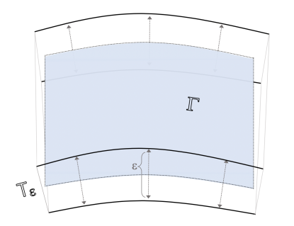
Figure 1. New Optimal Transport problems $\text{OT}_{\epsilon}$ will be defined on $T_{\epsilon}$ of $\Gamma$ to have solutions to the Optimal Transport problems (OTs) on $\Gamma$.

3.2. Extension of Surface Density Functions to $T_{\epsilon}$

Let $f\in\Theta_{\Gamma}$, we can rewrite the integration of $f$ on $\Gamma$ to one on $\Gamma_{y}$ for any $y\in(\epsilon,\epsilon)$ as follows:

(17) $$\int_{\Gamma}f(\mathbf{x})dS=\int_{\Gamma_{y}}f(P_{\Gamma}\mathbf{z}^{\prime})J(\mathbf{z}^{\prime})dS,$$

where $J(\mathbf{z}^{\prime})=(1-\kappa_{1}y)(1-\kappa_{2}y)$ accounts for the change of variables in the integrations. See e.g. [15]. Furthermore, by the coarea formula,

$$1=\int_{\Gamma}f(\mathbf{x})dS=\frac{1}{2\epsilon}\int_{-\epsilon}^{\epsilon}\int_{\Gamma_{y}}f(P_{\Gamma}\mathbf{z}^{\prime})J(\mathbf{z}^{\prime})dSdy =\frac{1}{2\epsilon}\int_{T_{\epsilon}}f(P_{\Gamma}\mathbf{z})J(\mathbf{z})d\mathbf{z}.$$

Therefore, our extended Optimal Transport problem is formulated with the class of density function defined below:

(18) $$\Theta_{T_{\epsilon}}:=\left\{\frac{1}{2\epsilon}\rho(P_{\Gamma}\mathbf{z})J(\mathbf{z}):\rho\in\Theta_{\Gamma}\right\}.$$

Therefore, any density in $\Theta_{T_{\epsilon}}$ is strictly positive and smooth (The Jacobian $J$ is smooth and strictly positive since we stay within the reach of $\Gamma$.)

3.3. Extension of Cost Function to $T_{\epsilon}$

Let $c$ be the cost function defined on $\Gamma$. We define the extended cost function for any two points in $T_{\epsilon}$ by adding an additional cost to the difference in their distance to $\Gamma$:

(19) $$c_{\epsilon}(\mathbf{z}_{1},\mathbf{z}_{2})=c(P_{\Gamma}\mathbf{z}_{1},P_{\Gamma}\mathbf{z}_{2})+\frac{\sigma}{2}(\phi_{\Gamma}(\mathbf{z}_{1})-\phi_{\Gamma}(\mathbf{z}_{2}))^{2},$$

for $\sigma>0$. We will see that the particular choice of $\sigma$ will not affect the analysis.

3.4. Equivalence of the Two Optimal Transport Problems

In this section, we establish that the Optimal Transport problem defined via our extensions of the density functions and the cost function in Sections 3.2 and 3.3 leads to an Optimal Transport mapping $\mathbf{m}_{\epsilon}$ that moves mass only along each level set of the distance function to $\Gamma$. Moreover, $\mathbf{m}_{\epsilon}$ can be used to find $\mathbf{m}$, the mapping from the Optimal Transport problem on $\Gamma$.

Theorem 4.

The solution, $\mathbf{m}_{\epsilon}$, to the new Optimal Transport problem presented in Equation (9) defined with the densities in $\Theta_{T_{\epsilon}}$ and cost function in Equation (19), satisfies

(20) $$P_{\Gamma}\mathbf{m}_{\epsilon}(\mathbf{z})=\mathbf{m}(P_{\Gamma}\mathbf{z}),~{}~{}~{}\forall\mathbf{z}\in T_{\epsilon},$$

and

(21) $$\phi_{\Gamma}(\mathbf{z})=\phi_{\Gamma}(\mathbf{m}_{\epsilon}(\mathbf{z})),~{}~{}~{}\forall\mathbf{z}\in T_{\epsilon}.$$

This theorem then implies that the Optimal Transport cost for the Optimal Transport problem on $\Gamma$ is equal to the Optimal Transport cost for the extended Optimal Transport problem on $T_{\epsilon}$. Thus, the Wasserstein distance, for example, on $\Gamma$ can be computed via the extended Optimal Transport problem on $T_{\epsilon}$.

Corollary 5.

We have

(22) $$\min_{\boldsymbol{\xi}_{\#}\mu_{\epsilon}=\nu_{\epsilon}}\int_{T_{\epsilon}}c_{\epsilon}(\mathbf{z},\boldsymbol{\xi}(\mathbf{z}))f_{\epsilon}(\mathbf{z})d\mathbf{z}=\min_{\boldsymbol{\theta}_{\#}\mu=\nu}\int_{\Gamma}c(\mathbf{x},\boldsymbol{\theta}(\mathbf{x}))f(\mathbf{x})dS(\mathbf{x}).$$

Proof.

$$\min_{\boldsymbol{\xi}_{\#}\mu_{\epsilon}=\nu_{\epsilon}}\int_{T_{\epsilon}}c_{\epsilon}(\mathbf{z},\boldsymbol{\xi})f_{\epsilon}(\mathbf{z})d\mathbf{z} =\int_{T_{\epsilon}}c_{\epsilon}(\mathbf{z},\mathbf{m}_{\epsilon})f_{\epsilon}(\mathbf{z})d\mathbf{z}$$

$$=\int_{T_{\epsilon}}c(P_{\Gamma}\mathbf{z},P_{\Gamma}\mathbf{m}_{\epsilon})f_{\epsilon}(\mathbf{z})d\mathbf{z}$$

$$=\frac{1}{2\epsilon}\int_{-\epsilon}^{\epsilon}\int_{\Gamma_{y}}c(P_{\Gamma}\mathbf{z},P_{\Gamma}\mathbf{m}_{\epsilon}(\mathbf{z}))f(\mathbf{x})J(\mathbf{z})dS(\mathbf{z})dy$$

$$=\frac{1}{2\epsilon}\int_{-\epsilon}^{\epsilon}\int_{\Gamma}c(\mathbf{x},\mathbf{m}(\mathbf{x}))f(\mathbf{x})dS(\mathbf{x})dy$$

$$=\int_{\Gamma}c(\mathbf{x},\mathbf{m}(\mathbf{x}))f(\mathbf{x})dS(\mathbf{x})$$

$$=\min_{\boldsymbol{\theta}_{\#}\mu=\nu}\int_{\Gamma}c(\mathbf{x},\boldsymbol{\theta}(\mathbf{x}))f(\mathbf{x})dS(\mathbf{x}).$$

∎

Mass preservation

Since $\epsilon<\tau_{\Gamma}$ and $\Gamma$ is compact and closed, the projection $P_{\Gamma}$ is bijective between $\Gamma$ and $\Gamma_{y}$ for any $y\in(-\epsilon,\epsilon).$ We define the inverse map

(23) $$P_{\Gamma,\Gamma_{y}}^{-1}(\mathbf{z}):=\mathbf{z}+y\mathbf{n}(\mathbf{z}),~{}~{}~{}\text{for}~{}\mathbf{z}\in\Gamma,$$

where $\mathbf{n}(\mathbf{z})=\nabla\phi_{\Gamma}(\mathbf{z})$ is the outward normal vector of $\Gamma$ at $\mathbf{z}$. This vector remains the same for all $\mathbf{z}^{\prime}\in T_{\epsilon}$ satisfying $P_{\Gamma}\mathbf{z}^{\prime}=\mathbf{z}.$ Thus we see that $P_{\Gamma}\circ P^{-1}_{\Gamma,\Gamma_{y}}(\mathbf{z})=\mathbf{z}$ and $P^{-1}_{\Gamma,\Gamma_{y}}\circ P_{\Gamma}(\mathbf{z}^{\prime})=\mathbf{z}^{\prime}$ for $\mathbf{z}^{\prime}\in\Gamma_{y}.$ Therefore, we can associate any mapping $\boldsymbol{\xi}:\Gamma\mapsto\Gamma$ with $\boldsymbol{\xi}\circ P_{\Gamma}:\Gamma_{y}\mapsto\Gamma_{y}$ and vice versa. So we define

(24) $$\boldsymbol{\xi}_{\epsilon}(\mathbf{z}):=P_{\Gamma,\Gamma_{y}}^{-1}\circ\boldsymbol{\xi}\circ P_{\Gamma}(\mathbf{z}),~{}~{}~{}\phi_{\Gamma}(\mathbf{z})=y,~{}~{}\text{and}~{}y\in(-\epsilon,\epsilon).$$

Equivalently,

(25) $$P_{\Gamma}\boldsymbol{\xi}_{\epsilon}(\mathbf{z}^{\prime})=\boldsymbol{\xi}(P_{\Gamma}\mathbf{z}^{\prime}),~{}~{}~{}\mathbf{z}\in T_{\epsilon},$$

and

(26) $$\phi_{\Gamma}(\boldsymbol{\xi}_{\epsilon}(\mathbf{z}^{\prime}))=\phi_{\Gamma}(\boldsymbol{\xi}_{\epsilon}(\mathbf{z}^{\prime})),~{}~{}~{}\mathbf{z}\in T_{\epsilon}.$$

In particular, suppose $\mathbf{m}$ is the solution to the Optimal transport problem in Equation (3) on $\Gamma$. Then, we will show that

(27) $$\tilde{\mathbf{m}}_{\epsilon}(\mathbf{z}):=(P_{\Gamma}\mathbf{z}+\phi_{\Gamma}(\mathbf{z})\mathbf{n}(\mathbf{z}))~{}\mathbf{m}(P_{\Gamma}\mathbf{z})$$

is a solution to the extended Optimal Transport problem in Equation (9).

The first step is to show that if $\boldsymbol{\xi}\#\mu=\nu$ with $\mu=fdS$ and $\nu=gdS$, then $\boldsymbol{\xi}_{\epsilon}\mu_{\epsilon}=\nu_{\epsilon}$, with $\mu_{\epsilon}=f_{\epsilon}d\mathbf{x}$, and $\nu_{\epsilon}=g_{\epsilon}d\mathbf{x}$. But this is another exercise on the coarea formula. Let $E\subset T_{\epsilon}$, we have

$$\int_{E}g_{\epsilon}(\mathbf{x})d\mathbf{x} =\int_{-\epsilon}^{\epsilon}\int_{E\cap\Gamma_{y}}g(P_{\Gamma}\mathbf{z}^{\prime})J(\mathbf{z}^{\prime})dS~{}dy$$

$$=\int_{-\epsilon}^{\epsilon}\int_{P_{\Gamma}(E\cap\Gamma_{y})}g(\mathbf{z})dSdy$$

$$=\int_{-\epsilon}^{\epsilon}\int_{\boldsymbol{\xi}^{-1}(P_{\Gamma}(E\cap\Gamma_{y}))}f(\mathbf{z})dSdy$$

$$=\int_{-\epsilon}^{\epsilon}\int_{P^{-1}_{\Gamma,\Gamma_{y}}(\boldsymbol{\xi}^{-1}(P_{\Gamma}(E\cap\Gamma_{y})))}f(P_{\Gamma}\mathbf{z})J(\mathbf{z})dSdy$$

$$=\int_{-\epsilon}^{\epsilon}\int_{\boldsymbol{\xi}_{\epsilon}^{-1}(E\cap\Gamma_{y})}f(P_{\Gamma}\mathbf{z}^{\prime})J(\mathbf{z}^{\prime})dS~{}dy=\int_{\boldsymbol{\xi}_{\epsilon}^{-1}(E)}f_{\epsilon}(\mathbf{x})d\mathbf{x},$$

where the penultimate equality follows since $P_{\Gamma,\Gamma_{y}}^{-1}\circ\boldsymbol{\xi}^{-1}\circ P_{\Gamma}\circ P^{-1}_{\Gamma,\Gamma_{y}}\circ\boldsymbol{\xi}\circ P_{\Gamma}=P_{\Gamma,\Gamma_{y}}^{-1}\circ\boldsymbol{\xi}^{-1}\circ\boldsymbol{\xi}\circ P_{\Gamma}=P_{\Gamma,\Gamma_{y}}^{-1}\circ P_{\Gamma}=\text{Id}$, we then know that $P^{-1}_{\Gamma,\Gamma_{y}}(\boldsymbol{\xi}^{-1}(P_{\Gamma}(E\cap\Gamma_{y})))=\boldsymbol{\xi}_{\epsilon}^{-1}(E\cap\Gamma_{y})$.

Comparing Equation (9) with Equation (19), Equation (17), and Equation (18), we see that the transport cost over all $\boldsymbol{\xi}_{\epsilon}$ is minimized for $\boldsymbol{\xi}_{\epsilon}=\tilde{\mathbf{m}}_{\epsilon}$:

(28) $$\int_{T_{\epsilon}}c_{\epsilon}\left(\mathbf{z}^{\prime},\boldsymbol{\xi}_{\epsilon}(\mathbf{z}^{\prime})\right)f_{\epsilon}(\mathbf{z}^{\prime})d\mathbf{z}^{\prime}$$

$$=\int_{-\epsilon}^{\epsilon}\int_{\Gamma_{y}}c(P_{\Gamma}\mathbf{z}^{\prime},P_{\Gamma}\boldsymbol{\xi}_{\epsilon}(\mathbf{z}^{\prime}))f(P_{\Gamma}\mathbf{z}^{\prime})J(\mathbf{z}^{\prime})dSdy$$

$$=2\epsilon\int_{\Gamma}c(\mathbf{z},\boldsymbol{\xi}(\mathbf{z}))f(\mathbf{z})dS$$

$$\geq 2\epsilon\int_{\Gamma}c(\mathbf{z},\boldsymbol{m}(\mathbf{z}))f(\mathbf{z})dS=\int_{T_{\epsilon}}c_{\epsilon}\left(\mathbf{z}^{\prime},\tilde{\boldsymbol{m}}_{\epsilon}(\mathbf{z}^{\prime})\right)f_{\epsilon}(\mathbf{z}^{\prime})d\mathbf{z}^{\prime},$$

Following the above construction, we see that Equation (20) holds for $\tilde{\mathbf{m}}_{\epsilon}$. Now consider $\mathbf{z}_{y}\in\Gamma_{y}$. By construction, $\tilde{\mathbf{m}}_{\epsilon}(\mathbf{z}_{y})\in\Gamma_{y},$ implying Equation (21). $\tilde{\mathbf{m}}_{\epsilon}(\mathbf{z})$ does not move mass in the normal direction of $\Gamma$.

For our extended problem, since the source and target densities are supported on $\mathbb{R}^{3}$, the Optimal Mapping $\mathbf{m}_{\epsilon}$ and potential function $u_{\epsilon}$ satisfy:

(29) $$\nabla u_{\epsilon}(\mathbf{z})=-\nabla_{\mathbf{z}}c_{\epsilon}(\mathbf{z},\boldsymbol{\xi}),$$

for $\boldsymbol{\xi}=\mathbf{m}_{\epsilon}(\mathbf{z})$, where we emphasize that $\nabla$ is the Euclidean gradient and $u_{\epsilon}$ is $c_{\epsilon}$ convex. The relation defined in Equation (29) applied to $\tilde{\mathbf{m}}_{\epsilon}$ and separated into one defined on surfaces that are equidistant to $\Gamma$ becomes

(30) $$(I-\mathbf{n}\otimes\mathbf{n})\nabla\tilde{u}_{\epsilon}(\mathbf{z})=-(I-\mathbf{n}\otimes\mathbf{n})\nabla_{\mathbf{z}}c\left(P_{\Gamma}\mathbf{z},\mathbf{m}\right),$$

and one in the normal direction of the surface,

(31) $$\nabla\tilde{u}_{\epsilon}(\mathbf{z})\cdot\mathbf{n}=\sigma\left(\phi_{\Gamma}((\tilde{\mathbf{m}}_{\epsilon}(\mathbf{z}))-\phi_{\Gamma}(\mathbf{z})\right).$$

Here $\mathbf{n}$ is the normal of $\Gamma$ at $P_{\Gamma}\mathbf{z}$. Notice that for $\mathbf{z}\in\Gamma$, Equation (30) is Equation (6). This means that the restriction of $u_{\epsilon}$ on $\Gamma$ solves Equation (6).

Using Equation (21) in Equation (31), we obtain

(32) $$\frac{\partial\tilde{u}_{\epsilon}}{\partial\mathbf{n}}(\mathbf{z})=0,~{}~{}~{}\mathbf{z}\in T_{\epsilon}.$$

Then, by Equation (30)

$$u_{\epsilon}(\mathbf{z})=u(P_{\Gamma}\mathbf{z})+C,$$

for some constant $C$ and $P_{\Gamma}\mathbf{m}_{\epsilon}(\mathbf{z})=\mathbf{m}(P_{\Gamma}\mathbf{z})$, which is the solution pair from the Optimal Transport problem on $\Gamma$.

Now, in order to finish the proof of Theorem 4, it remains to show that $\tilde{u}_{\epsilon}$ is $c_{\epsilon}$-convex. Once this is shown, then by Theorem 3 there is a unique solution of the Optimal Transport problem in Equation (9), then we have shown, in fact, $\tilde{\mathbf{m}}_{\epsilon}=\mathbf{m}_{\epsilon}$ satisfying $\phi_{\Gamma}(\mathbf{m}_{\epsilon}(\mathbf{z}))=\phi_{\Gamma}(\mathbf{z})$ and $P_{\Gamma}\mathbf{m}_{\epsilon}(\mathbf{z})=\mathbf{m}(P_{\Gamma}\mathbf{z})$.

$c_{\epsilon}$-Convexity of the Potential Function

Lemma 6.

$\tilde{u}_{\epsilon}(\mathbf{z})=u(P_{\Gamma}\mathbf{z})$ is $c_{\epsilon}$-convex.

Proof.

Recall the definition of $c$-convexity from Definition 2: $u$ is $c$ convex since it is the potential function for the Optimal Transport problem on $\Gamma$. This means that for all $\mathbf{x}\in\Gamma$, there exists a point $\mathbf{\tilde{x}}\in\Gamma$ and the $c$-transform of $u$ satisfies $u^{c}(\mathbf{\tilde{x}})$ such that:

(33) $$-u^{c}(\mathbf{\tilde{x}})-c(\mathbf{x},\mathbf{\tilde{x}}) =u(\mathbf{x}),$$

(34) $$-u^{c}(\mathbf{\tilde{x}})-c(\mathbf{x}^{\prime},\mathbf{\tilde{x}}) \leq u(\mathbf{x}^{\prime}),\ \forall\mathbf{x}^{\prime}\in\Gamma.$$

Now, fix $\mathbf{x}\in\Gamma$ and fix a $\mathbf{z}\in T_{\epsilon}$ such that $P_{\Gamma}\mathbf{z}=\mathbf{x}$. From Equation (33), given $\mathbf{x}\in\Gamma$, we have an $\tilde{\mathbf{x}}\in\Gamma$ such that Equation (33) holds. Choose $\tilde{\mathbf{z}}$ such that $P_{\Gamma}\tilde{\mathbf{x}}=\tilde{\mathbf{x}}$ and $\phi_{\Gamma}\tilde{\mathbf{z}}=\phi_{\Gamma}\mathbf{z}$. By the definition of the $c$-transform in $T_{\epsilon}$:

(35) $$\tilde{u}^{c_{\epsilon}}_{\epsilon}(\mathbf{\tilde{z}})=\sup_{\boldsymbol{\xi}}\left(-c_{\epsilon}(\boldsymbol{\xi},\mathbf{\tilde{z}})-\tilde{u}_{\epsilon}(\boldsymbol{\xi})-C\right),$$

(36) $$=\sup_{P_{\Gamma}\boldsymbol{\xi,\phi_{\Gamma}\boldsymbol{\xi}}}\left(-c(P_{\Gamma}\boldsymbol{\xi},\mathbf{\tilde{x}})-\frac{\sigma}{2}(\phi_{\Gamma}\boldsymbol{\xi}-\phi_{\Gamma}\tilde{\mathbf{z}})^{2}-u(P_{\Gamma}\boldsymbol{\xi})-C\right),$$

we can immediately take the supremum over $\phi_{\Gamma}\boldsymbol{\xi}$ by choosing $\phi_{\Gamma}\boldsymbol{\xi}=\phi_{\Gamma}\tilde{\mathbf{z}}$, since the other terms do not depend on $\phi_{\Gamma}\boldsymbol{\xi}$. Thus,

(37) $$\tilde{u}^{c_{\epsilon}}_{\epsilon}(\mathbf{\tilde{z}})=\sup_{P_{\Gamma}\boldsymbol{\xi}}\left(-c(P_{\Gamma}\boldsymbol{\xi},\mathbf{\tilde{x}})-u(P_{\Gamma}\boldsymbol{\xi})-C\right)=u^{c}(\mathbf{\tilde{x}})-C.$$

Thus, we get:

(38) $$-\tilde{u}_{\epsilon}^{c_{\epsilon}}(\mathbf{\tilde{z}})-c_{\epsilon}(\mathbf{z},\mathbf{\tilde{z}})=-u^{c}(\mathbf{\tilde{x}})-C-c(P_{\Gamma}\mathbf{z},\mathbf{\tilde{x}})=u(P_{\Gamma}\mathbf{z})-C=\tilde{u}_{\epsilon}(\mathbf{z}),$$

by Equation (33). Now, for any $\mathbf{z}^{\prime}\in T_{\epsilon}$. Then,

(39) $$-\tilde{u}_{\epsilon}^{c_{\epsilon}}(\mathbf{\tilde{z}})-c_{\epsilon}(\mathbf{z}^{\prime},\mathbf{\tilde{z}})=-u^{c}(\mathbf{\tilde{x}})-C-\frac{\sigma}{2}(\phi_{\Gamma}\mathbf{z}^{\prime}-\phi_{\Gamma}\tilde{\mathbf{z}})^{2}-c(P_{\Gamma}\mathbf{z}^{\prime},P_{\Gamma}\tilde{\mathbf{z}})\leq\\ -u^{c}(\mathbf{\tilde{x}})-C-c(P_{\Gamma}\mathbf{z}^{\prime},P_{\Gamma}\tilde{\mathbf{z}})\leq u(P_{\Gamma}\mathbf{z}^{\prime})-C=\tilde{u}_{\epsilon}(\mathbf{z}^{\prime}),\ \forall\mathbf{z}^{\prime},$$

by Equation (34). Thus, $\tilde{u}_{\epsilon}$ is $c_{\epsilon}$-convex.

∎

3.5. Example: Optimal Transport on the Unit Sphere

We have just discussed the general procedure for defining a new Optimal Transport problem on $T_{\epsilon}$, which uses coordinate-free notation. Here, we narrow our scope to show, specifically, how some quantities discussed earlier in this section can be computed for the case of the sphere $\Gamma=\mathbb{S}^{2}$ with a specific coordinate system. We also compute various quantities for two specific cost functions, the squared geodesic cost function $c(\mathbf{x},\mathbf{y})=\frac{1}{2}d_{\mathbb{S}^{2}}(\mathbf{x},\mathbf{y})^{2}$ and the logarithmic cost function $c(\mathbf{x},\mathbf{y})=-\log(1-\mathbf{x}\cdot\mathbf{y})$ arising in the reflector antenna problem. This allows us to derive concrete formulas, which we can then use in our discretizations in Section 4, where computations are performed on the unit sphere for both cost functions.

We show how the Optimal Transport problem in Equation (3) on the unit sphere $\mathbb{S}^{2}\subset\mathbb{R}^{3}$ is extended. We will use the usual spherical polar coordinates $(\phi,\theta,r)$ in our calculation: $\mathbf{z}=(r\cos\phi\sin\theta,r\sin\phi\sin\theta,r\cos\theta)$. $\Gamma$ consists of the set of points whose $r$ coordinate is $1$. For any point other than the origin, $P_{\Gamma}\mathbf{z}=\mathbf{z}/||\mathbf{z}||$, $\mathbf{z}=(\phi,\theta,r)$, $\phi_{\Gamma}(\mathbf{z})=1-r$, $J=1/r^{2}$, $dS=\sin\theta d\phi d\theta$, and the surface gradient $\nabla_{\mathbb{S}^{2}}u=\frac{1}{\sin^{2}\theta}\frac{\partial u(\phi,\theta)}{\partial\phi}\hat{\phi}+\frac{\partial u(\phi,\theta)}{\partial\theta}\hat{\theta}$, where $\hat{\phi}=(-\sin\phi,\cos\phi,0)$ and $\hat{\theta}=(\cos\phi\cos\theta,\sin\phi,\cos\theta,-\sin\theta)$.

The densities on $T_{\epsilon}$ are defined:

(40) $$f_{\epsilon}(\phi,\theta,r) =\frac{f(\phi,\theta)}{2\epsilon r^{2}},$$

(41) $$g_{\epsilon}(\phi,\theta,r) =\frac{g(\phi,\theta)}{2\epsilon r^{2}}.$$

Now we define the cost function $c_{\epsilon}$ in $T_{\epsilon}$ as follows for $\mathbf{z}=(\phi_{1},\theta_{1},r_{1})$ and $\boldsymbol{\xi}=(\phi_{2},\theta_{2},r_{2})$:

(42) $$c_{\epsilon}(\mathbf{z},\boldsymbol{\xi})=\frac{\sigma}{2}(r_{1}-r_{2})^{2}+c\left(\frac{\mathbf{z}}{r_{1}},\frac{\boldsymbol{\xi}}{r_{2}}\right).$$

For the squared geodesic cost function on the sphere $c(\mathbf{x},\mathbf{y})=\frac{1}{2}\arccos(\mathbf{x}\cdot\mathbf{y})^{2}$, we have explicitly:

(43) $$c_{\epsilon}(\mathbf{z},\boldsymbol{\xi})=\frac{\sigma}{2}(r_{1}-r_{2})^{2}+\frac{1}{2}\arccos\left(\frac{\mathbf{z}}{r_{1}}\cdot\frac{\boldsymbol{\xi}}{r_{2}}\right)^{2},$$

and for the logarithmic cost $c(\mathbf{x},\mathbf{y})=-\log(1-\mathbf{x}\cdot\mathbf{y})$, we have:

(44) $$c_{\epsilon}(\mathbf{z},\boldsymbol{\xi})=\frac{\sigma}{2}(r_{1}-r_{2})^{2}-\log\left(1-\frac{\mathbf{z}}{r_{1}}\cdot\frac{\boldsymbol{\xi}}{r_{2}}\right)^{2}.$$

Denoting $\mathbf{m}=(m_{\phi},m_{\theta},1)$ to be the $(\phi,\theta,r)$ coordinates of the solution of the original Optimal Transport problem on $\Gamma=\mathbb{S}^{2}$ in Equation (3), we have shown, in Theorem 4 that $\mathbf{m}_{\epsilon}$ has the following form in spherical coordinates:

(45) $$\mathbf{m}_{\epsilon}(\phi,\theta,r)=\left(m_{\phi},m_{\theta},r\right).$$

Here we remind the reader the explicit form of the Optimal Transport mapping from Equation (3) for the squared geodesic cost function $c(\mathbf{x},\mathbf{y})=\frac{1}{2}d_{\mathbb{S}^{2}}(\mathbf{x},\mathbf{y})^{2}$. We get it by solving Equation (6). It is related to the potential function via the following equation:

(46) $$\mathbf{m}(\mathbf{x})=\text{exp}_{\mathbf{x}}\left(\nabla_{\mathbb{S}^{2}}u(\mathbf{x})\right).$$

which is a particular case of a result that is well known due to McCann [23]. The notation in Equation (46) means that to get to the point $\mathbf{m}(\mathbf{x})\in\mathbb{S}^{2}$ from $\mathbf{x}$ we follow the geodesic on $\mathbb{S}^{2}$ (on the great circle through $\mathbf{x}$) starting from $\mathbf{x}$ in the direction $\nabla u(\mathbf{x})$ a distance of $\left\|\nabla u(\mathbf{x})\right\|$. Alternatively, we can write:

(47) $$\mathbf{m}(\mathbf{x})=\text{exp}_{\mathbf{x}}\left(\nabla_{\mathbb{S}^{2}}u(\mathbf{x})\right)=\mathbf{x}\cos(\left\|\nabla_{\mathbb{S}^{2}}u(\mathbf{x})\right\|)+\frac{\nabla_{\mathbb{S}^{2}}u(\mathbf{x})}{\left\|\nabla_{\mathbb{S}^{2}}u(\mathbf{x})\right\|}\sin(\left\|\nabla_{\mathbb{S}^{2}}u(\mathbf{x})\right\|).$$

For the logarithmic cost function appearing in the reflector antenna problem, $c(x,y)=-\log(1-\mathbf{x}\cdot\mathbf{y})$, we get the mapping [13]:

(48) $$\mathbf{m}(\mathbf{x})=\mathbf{x}\frac{\left\|\nabla_{\mathbb{S}^{2}}u(\mathbf{x})\right\|^{2}-1}{\left\|\nabla_{\mathbb{S}^{2}}u(\mathbf{x})\right\|^{2}+1}-\nabla_{\mathbb{S}^{2}}u(\mathbf{x})\frac{2}{\left\|\nabla_{\mathbb{S}^{2}}u(\mathbf{x})\right\|^{2}+1}.$$

Following the computational methods developed in [12] and [13], we also can explicitly derive the formulas for the quantity in Equation (7) for the squared geodesic cost function $c(\mathbf{x},\mathbf{y})=\frac{1}{2}d_{\mathbb{S}^{2}}(\mathbf{x},\mathbf{y})^{2}$:

(49) $$\left|\det D^{2}_{\mathbf{x}\mathbf{y},\mathbb{S}^{2}}\left(\frac{1}{2}d_{\mathbb{S}^{2}}(\mathbf{x},\mathbf{y})^{2}\right)\right|=\frac{\left\|\nabla_{\mathbb{S}^{2}}u(\mathbf{x})\right\|}{\sin\left(\left\|\nabla_{\mathbb{S}^{2}}u(\mathbf{x})\right\|\right)},$$

for $\mathbf{y}=\mathbf{m}(\mathbf{x})$ given in Equation (47). For the logarithmic cost $c(\mathbf{x},\mathbf{y})=-\log(1-\mathbf{x}\cdot\mathbf{y})$:

(50) $$\left|\det D^{2}_{\mathbf{x}\mathbf{y},\mathbb{S}^{2}}\left(-\log(1-\mathbf{x}\cdot\mathbf{y})\right)\right|=\frac{\left(\left\|\nabla_{\mathbb{S}^{2}}u(\mathbf{x})\right\|^{2}+1\right)^{2}}{4},$$

for $\mathbf{y}=\mathbf{m}(\mathbf{x})$ given in Equation (48).

Therefore, for both cost functions, the term $\left|D^{2}_{\mathbf{z}\boldsymbol{\xi}}c_{\epsilon}(\mathbf{z},\boldsymbol{\xi})\right|$ for $\boldsymbol{\xi}=\mathbf{m}_{\epsilon}(\mathbf{z})$ from Equation (10) can be computed explicitly via the methods developed in [12] and via Equation (49) and Equation (50). The result for the cost function $c_{\epsilon}(\mathbf{z}_{1},\mathbf{z}_{2})=c(P_{\Gamma}\mathbf{z}_{1},P_{\Gamma}\mathbf{z}_{2})+\frac{\sigma}{2}(\phi_{\Gamma}(\mathbf{z}_{1})-\phi_{\Gamma}(\mathbf{z}_{2}))^{2}$ for $c(\mathbf{x},\mathbf{y})=\frac{1}{2}d_{\mathbb{S}^{2}}(\mathbf{x},\mathbf{y})^{2}$ is:

(51) $$\left|\det D^{2}_{\mathbf{z}\boldsymbol{\xi}}c_{\epsilon}(\mathbf{z},\mathbf{x}_{i})\right|=\sigma\frac{\left\|\nabla u_{\epsilon}(\mathbf{z})-\left(\nabla u_{\epsilon}(\mathbf{z})\cdot\frac{\mathbf{z}}{\left\|\mathbf{z}\right\|}\right)\frac{\mathbf{z}}{\left\|\mathbf{z}\right\|}\right\|}{\left\|\mathbf{z}\right\|^{2}\sin\left(\left\|\nabla u_{\epsilon}(\mathbf{z})-\left(\nabla u_{\epsilon}(\mathbf{z})\cdot\frac{\mathbf{z}}{\left\|\mathbf{z}\right\|}\right)\frac{\mathbf{z}}{\left\|\mathbf{z}\right\|}\right\|\right)},$$

for $\boldsymbol{\xi}=\mathbf{m}_{\epsilon}(\mathbf{z})$. For the logarithmic cost $c(\mathbf{x},\mathbf{y})=-\log(1-\mathbf{x}\cdot\mathbf{y})$, we get:

(52) $$\left|\det D^{2}_{\mathbf{z}\boldsymbol{\xi}}c_{\epsilon}(\mathbf{z},\boldsymbol{\xi})\right|=\frac{\sigma\left(\left\|\nabla u_{\epsilon}(\mathbf{x})-\left(\nabla u_{\epsilon}(\mathbf{z})\cdot\frac{\mathbf{z}}{\left\|\mathbf{z}\right\|}\right)\frac{\mathbf{z}}{\left\|\mathbf{z}\right\|}\right\|^{2}+1\right)^{2}}{4\left\|\mathbf{z}\right\|^{2}},$$

for $\boldsymbol{\xi}=\mathbf{m}_{\epsilon}(\mathbf{z})$.

4. Computational Examples

The key innovation in reformulating the Optimal Transport problem on $T_{\epsilon}$ is to allow for a wide selection of numerical discretizations for $T_{\epsilon}$ and the PDE (10) defined on it. In this section, we discuss a simple method for solving the PDE (10) and demonstrate some computational results using the method. Mainly for the sake of convenience, we use simple finite differences on uniform Cartesian grids (although we emphasize that it is possible to use other types of discretizations), and demonstrate the computational results for the sphere $\Gamma=\mathbb{S}^{2}$. For most examples we use the squared geodesic cost function $c(\mathbf{x},\mathbf{y})=\frac{1}{2}d_{\mathbb{S}^{2}}(\mathbf{x},\mathbf{y})^{2}$. We will also demonstrate the results of one computation using the cost function $c(\mathbf{x},\mathbf{y})=-\log(1-\mathbf{x}\cdot\mathbf{y})$ arising in the reflector antenna problem, see [36, 37]. We perform this computation in order to show that our formulation in Section 3 will work for a variety of cost functions on the sphere. Given that we are using finite-difference discretizations on a Cartesian grid, it is also straightforward to design higher-order discretizations than those which we present here.

4.1. Description of Scheme

In this section, since our discretization is constructed on a Cartesian grid, we use the notation $x,y,z$ to denote the usual Cartesian coordinates $(x,y,z)\in\mathbb{R}^{3}$. In order to discretize Equation (10), we first generate a cube of $N_{c}$ points placed on an evenly spaced Cartesian grid $\mathcal{G}_{c}^{h}\subset\mathbb{R}^{3}$, where the discretization parameter $h$ satisfies $h=\min_{i,j}\left\|\mathbf{x}_{i}-\mathbf{x}_{j}\right\|$ for $j\neq i,\mathbf{x}_{i},\mathbf{x}_{j}\in\mathcal{G}^{h}_{c}$. The computational grid $\mathcal{G}^{h}$ of $N$ points is then generated by taking the intersection of the cube grid with the tubular neighborhood $T_{\epsilon}$ of the surface $\Gamma=\mathbb{S}^{2}$, i.e. $\mathcal{G}^{h}=\mathcal{G}^{h}_{c}\cap T_{\epsilon}$. We designate interior points $\mathbf{x}_{i}=(x,y,z)$ as those surrounded by computational points in the computational grid. These neighboring points will be used in the computation of the first and second discrete derivatives in Equation (10), and thus interior points are those where these derivatives can be computed.

Definition 7.

A point $\mathbf{x}_{i}\in\mathcal{G}^{h}$ will be called an interior point iff $\mathbf{x}_{i}+(\eta_{1}h,\eta_{2}h,\eta_{3}h)\in\mathcal{G}^{h}$, where $\eta_{i}\in\left\{-1,0,1\right\}$ and $\eta_{1}\eta_{2}\eta_{3}=0$.

Boundary points, consequently, are those which are not interior points. The interior points are the points at which we will be able to fully discretize the PDE operator and the boundary points are the points at which we will apply the boundary condition in Equation (12). Since the solution $u_{\epsilon}$ of Equation (10) is a priori constant in the normal direction, we elect to enforce the condition $u(\mathbf{x}_{i})=u(\mathbf{x}_{i}/\left\|\mathbf{x}_{i}\right\|)$, for any boundary point $\mathbf{x}_{i}$. We denote the set interior points by $\mathcal{I}^{h}\subset\mathcal{G}^{h}$ and the set of boundary points by $\mathcal{B}^{h}\subset\mathcal{G}^{h}$. An example of the computational grid, as well as the boundary points and interior points, is shown in Figure 2 for a grid with $40694$ points.

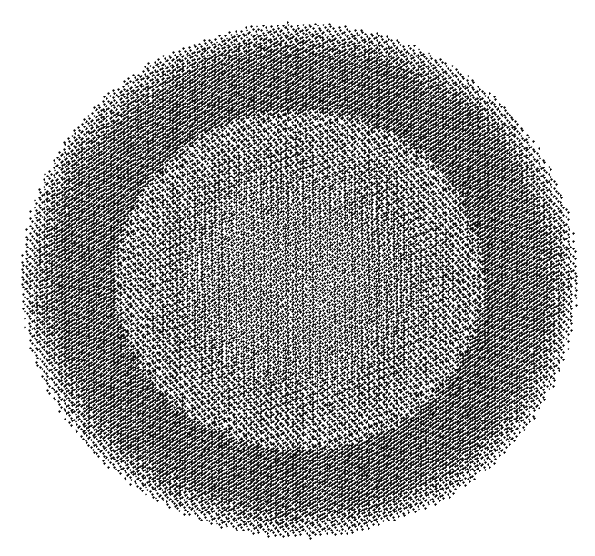
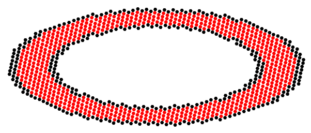
Figure 2. (a) An example of $40694$ Cartesian grid nodes in $T_{\epsilon}$, with $\epsilon=0.2$ and $h=0.05$. (b) A cross section showing the interior computational points in red.

For any function $f:T_{\epsilon}\rightarrow\mathbb{R}$, we use the following standard centered-difference discretization $\mathcal{D}^{h}_{1}f(\mathbf{x}_{i})$, $\mathcal{D}^{h}_{2}f(\mathbf{x}_{i})$, and $\mathcal{D}^{h}_{3}f(\mathbf{x}_{i})$ for the first-order derivatives $f_{x},f_{y},f_{z}$ at a point $\mathbf{x}_{i}$, respectively. Letting $\mathbf{e}_{1},\mathbf{e}_{2},\mathbf{e}_{3}$ denote $(1,0,0),(0,1,0)$, and $(0,0,1)$, respectively, we compute our first-order derivatives as follows:

$$\mathcal{D}^{h}_{j}f(\mathbf{x}_{i})=\frac{f(\mathbf{x}_{i}+h\mathbf{e}_{j})-f(\mathbf{x}_{i}-h\mathbf{e}_{j})}{2h},$$

and use the following discretization for the second-order derivatives:

$$\mathcal{D}^{h}_{jj}f(\mathbf{x}_{i})=\frac{f(\mathbf{x}_{i}+h\mathbf{e}_{j})-2f(\mathbf{x}_{i})+f(\mathbf{x}_{i}-h\mathbf{e}_{j})}{h^{2}},$$

and the following discretization for mixed second-order derivatives:

$$\mathcal{D}^{h}_{jk}f(\mathbf{x}_{i})=\frac{f(\mathbf{x}_{i}+h(\mathbf{e}_{j}+\mathbf{e}_{k}))+f(\mathbf{x}_{i}-h(\mathbf{e}_{j}+\mathbf{e}_{k}))}{h^{2}}-\\ \frac{f(\mathbf{x}_{i}+h(-\mathbf{e}_{j}+\mathbf{e}_{k}))+f(\mathbf{x}_{i}+h(\mathbf{e}_{j}-\mathbf{e}_{k}))}{h^{2}}.$$

These second-order derivatives are used in the computation of terms of the type $\det D^{2}F(\mathbf{x}_{i})$. Expanding out the determinant of the Hessian, we get

(53) $$\det D^{2}F(\mathbf{x}_{i})=F_{xx}\left(F_{yy}F_{zz}-F_{yz}^{2}\right)-F_{xy}\left(F_{xy}F_{zz}-F_{xz}F_{yz}\right)+F_{xz}\left(F_{xy}F_{yz}-F_{xz}F_{yy}\right).$$

We now proceed to show how we discretize the PDE (10). Given the potential function $u_{\epsilon}$, we first show how to compute the mapping $\mathbf{m}_{\epsilon}$. We compute the gradient via the equation

(54) $$\nabla^{h}u_{\epsilon}(\mathbf{x}_{i})=\mathcal{D}^{h}_{1}u_{\epsilon}(\mathbf{x}_{i})\mathbf{e}_{1}+\mathcal{D}^{h}_{2}u_{\epsilon}(\mathbf{x}_{i})\mathbf{e}_{2}+\mathcal{D}^{h}_{3}u_{\epsilon}(\mathbf{x}_{i})\mathbf{e}_{3}.$$

Using this, denote the unit normal vector $\hat{n}(\mathbf{x}_{i})=\mathbf{x}_{i}/\left\|\mathbf{x}_{i}\right\|$. Then, we compute the projection of the gradient onto the normal direction via the equation

(55) $$\mathcal{D}_{\hat{n}}^{h}u_{\epsilon}(\mathbf{x}_{i})=(\nabla^{h}u_{\epsilon}(\mathbf{x}_{i})\cdot\hat{n})\hat{n},$$

and the projection of the gradient onto the local tangent plane and scaled by the radius via

(56) $$\mathcal{D}_{\hat{n}^{\perp}}^{h}u_{\epsilon}(\mathbf{x}_{i})=\left\|\mathbf{x}_{i}\right\|\left(\nabla^{h}u_{\epsilon}(\mathbf{x}_{i})-\mathcal{D}_{\hat{n}}^{h}u_{\epsilon}(\mathbf{x}_{i})\right).$$

The mapping is computed from the projection of the gradient onto the local tangent plane via Equation (30). Therefore, from Equation (47), we see that for the squared geodesic cost $c(\mathbf{x},\mathbf{y})=\frac{1}{2}d_{\mathbb{S}^{2}}(\mathbf{x},\mathbf{y})^{2}$ we compute the mapping as follows:

(57) $$\mathbf{m}^{h}_{\epsilon}(\mathbf{x}_{i})=\\ \left(\mathbf{x}_{i}\cos\left(\left\|\mathcal{D}^{h}_{\hat{n}^{\perp}}u_{\epsilon}(\mathbf{x}_{i})\right\|\right)+\frac{\mathcal{D}^{h}_{\hat{n}^{\perp}}u_{\epsilon}(\mathbf{x}_{i})}{\left\|\mathcal{D}^{h}_{\hat{n}^{\perp}}u_{\epsilon}(\mathbf{x}_{i})\right\|}\sin\left(\left\|\mathcal{D}^{h}_{\hat{n}^{\perp}}u_{\epsilon}(\mathbf{x}_{i})\right\|\right)\right)\left(\left\|\mathbf{x}_{i}\right\|+\frac{\nabla^{h}u_{\epsilon}(\mathbf{x}_{i})\cdot\hat{n}}{\sigma}\right),$$

and from Equation (48), we compute the mapping for the logarithmic cost $c(\mathbf{x},\mathbf{y})=-\log(1-\mathbf{x}\cdot\mathbf{y})$ as follows:

(58) $$\mathbf{m}^{h}_{\epsilon}(\mathbf{x}_{i})=\left(\mathbf{x}_{i}\frac{\left\|\mathcal{D}^{h}_{\hat{n}^{\perp}}u_{\epsilon}(\mathbf{x}_{i})\right\|^{2}-1}{\left\|\mathcal{D}^{h}_{\hat{n}^{\perp}}u_{\epsilon}(\mathbf{x}_{i})\right\|^{2}+1}-\frac{2\mathcal{D}^{h}_{\hat{n}^{\perp}}u_{\epsilon}(\mathbf{x}_{i})}{\left\|\mathcal{D}^{h}_{\hat{n}^{\perp}}u_{\epsilon}(\mathbf{x}_{i})\right\|^{2}+1}\right)\left(\left\|\mathbf{x}_{i}\right\|+\frac{\nabla^{h}u_{\epsilon}(\mathbf{x}_{i})\cdot\hat{n}}{\sigma}\right).$$

In Equation (10), we also have the term $\left|\det D^{2}_{\mathbf{z}\boldsymbol{\xi}}c_{\epsilon}(\mathbf{z},\boldsymbol{\xi})\right|$ for $\boldsymbol{\xi}=\mathbf{m}_{\epsilon}(\mathbf{z})$, which can be discretized via Equation (54), Equation (55) and either Equation (51) for the squared geodesic cost or Equation (52) for the logarithmic cost.

In this way, we can fully discretize the PDE (10) for all interior points by defining the operator $F^{h}(u^{h}(\mathbf{x}_{i}))$ using Equation (59). For each interior point $\mathbf{x}_{i}$, first compute $\mathbf{m}^{h}_{\epsilon}(\mathbf{x}_{i})$. Then, for a point $\mathbf{C}\in T_{\epsilon}$, define $U_{\mathbf{C}}(\mathbf{z}):=u_{\epsilon}(\mathbf{z})+c_{\epsilon}(\mathbf{z},\mathbf{C})$. We then define $F^{h}$ for the squared geodesic cost $c(\mathbf{x},\mathbf{y})=\frac{1}{2}d_{\mathbb{S}^{2}}(\mathbf{x},\mathbf{y})^{2}$ as follows:

(59) $$F^{h}(u_{\epsilon}(\mathbf{x}_{i}))=\mathcal{D}^{h}_{11}U_{m^{h}_{\epsilon}(\mathbf{x}_{i})}(\mathbf{x}_{i})\left(\mathcal{D}^{h}_{22}U_{\mathbf{m}^{h}_{\epsilon}(\mathbf{x}_{i})}(\mathbf{x}_{i})\mathcal{D}^{h}_{33}U_{\mathbf{m}^{h}_{\epsilon}(\mathbf{x}_{i})}(\mathbf{x}_{i})-(\mathcal{D}^{h}_{23}U_{\mathbf{m}^{h}_{\epsilon}(\mathbf{x}_{i})}(\mathbf{x}_{i}))^{2}\right)-$$

$$\mathcal{D}^{h}_{12}U_{\mathbf{m}^{h}_{\epsilon}(\mathbf{x}_{i})}(\mathbf{x}_{i})\left(\mathcal{D}^{h}_{12}U_{\mathbf{m}^{h}_{\epsilon}(\mathbf{x}_{i})}(\mathbf{x}_{i})\mathcal{D}^{h}_{33}U_{\mathbf{m}^{h}_{\epsilon}(\mathbf{x}_{i})}(\mathbf{x}_{i})-\mathcal{D}^{h}_{13}U_{\mathbf{m}^{h}_{\epsilon}(\mathbf{x}_{i})}(\mathbf{x}_{i})\mathcal{D}^{h}_{23}U_{\mathbf{m}^{h}_{\epsilon}(\mathbf{x}_{i})}(\mathbf{x}_{i})\right)+$$

$$\mathcal{D}^{h}_{13}U_{\mathbf{m}^{h}_{\epsilon}(\mathbf{x}_{i})}(\mathbf{x}_{i})\left(\mathcal{D}^{h}_{12}U_{\mathbf{m}^{h}_{\epsilon}(\mathbf{x}_{i})}(\mathbf{x}_{i})\mathcal{D}^{h}_{23}U_{\mathbf{m}^{h}_{\epsilon}(\mathbf{x}_{i})}(\mathbf{x}_{i})-\mathcal{D}^{h}_{13}U_{\mathbf{m}^{h}_{\epsilon}(\mathbf{x}_{i})}(\mathbf{x}_{i})\mathcal{D}^{h}_{22}U_{\mathbf{m}^{h}_{\epsilon}(\mathbf{x}_{i})}(\mathbf{x}_{i})\right)-$$

$$\sigma\frac{\left\|\nabla^{h}u_{\epsilon}(\mathbf{x}_{i})-\mathcal{D}_{\hat{n}}^{h}u_{\epsilon}(\mathbf{x}_{i})\right\|f(\mathbf{x}_{i})}{\left\|\mathbf{x}_{i}\right\|^{2}\sin\left(\left\|\nabla^{h}u_{\epsilon}(\mathbf{x}_{i})-\mathcal{D}_{\hat{n}}^{h}u_{\epsilon}(\mathbf{x}_{i})\right\|\right)g(\mathbf{m}^{h}_{\epsilon}(\mathbf{x}_{i}))},$$

and we get a similar expression for the discretization of the PDE with the logarithmic cost $c(\mathbf{x},\mathbf{y})=-\log(1-\mathbf{x}\cdot\mathbf{y})$.

We then solve the following system of equations:

(60) $$F^{h}(u(\mathbf{x}_{i})) =0, \mathbf{x}_{i}\in\mathcal{I}^{h}$$

$$u(\mathbf{x}_{i}) =u(\mathbf{x}_{i}/\left\|\mathbf{x}_{i}\right\|), \mathbf{x}_{i}\in\mathcal{B}^{h}.$$

The boundary conditions are approximated by interpolation. For each boundary computational point $\mathbf{x}_{i}\in\mathcal{B}^{h}$, we compute the point $\boldsymbol{\xi}_{i}=\mathbf{x}_{i}/\left\|\mathbf{x}_{i}\right\|$. Denote its Euclidean coordinates by $(\xi_{i}^{x},\xi_{i}^{y},\xi_{i}^{z})$. We assume that $\epsilon$ and $h$ are chosen so that there is a point $\mathbf{p}_{i}\in\mathcal{G}^{h}$ with Euclidean coordinates $(p_{i}^{x},p_{i}^{y},p_{i}^{z})$ such that $\mathbf{p}_{i}=\operatorname*{argmin}_{p_{i}^{x}\>\xi_{i}^{x},p_{i}^{y}\>\xi_{i}^{y},p_{i}^{z}\>\xi_{i}^{z}}\left\|\boldsymbol{\xi}_{i}-\mathbf{p}_{i}\right\|$. Then, we define the list of points

$$R_{i}=\{\mathbf{p}_{i},\mathbf{p}_{i}-h\mathbf{e}_{1},\mathbf{p}_{i}-h\mathbf{e}_{2},\mathbf{p}_{i}-h\mathbf{e}_{3},\mathbf{p}_{i}-h(\mathbf{e}_{1}+\mathbf{e}_{2}),\mathbf{p}_{i}-h(\mathbf{e}_{1}+\mathbf{e}_{3}),\\ \mathbf{p}_{i}-h(\mathbf{e}_{2}+\mathbf{e}_{3}),\mathbf{p}_{i}-h(\mathbf{e}_{1}+\mathbf{e}_{2}+\mathbf{e}_{3})\}.$$

Assuming $\epsilon$ is thick enough with respect to $h$, the points in $R_{i}$ are in $\mathcal{G}^{h}$ and form the vertices of a small cube about $\boldsymbol{\xi}_{i}$.

In our discretization, we will then first update the interior points and then use the values of the new interior points to update the boundary points. To get the value of a function defined for all $\mathbf{x}_{i}\in\mathcal{G}^{h}$ at $\boldsymbol{\xi}_{i}$, we use trilinear interpolation using the values of the grid function at all points in $R_{i}$.

We choose to solve the discrete system (60) via Algorithm 1. Given $T_{\epsilon}$ and the Cartesian discretization, designate $I$ to be a list of the indices of the interior points and $B$ to be a list of the indices of the boundary points. This algorithm involves a Jacobi-style update, can thus can be trivially parallelized. Moreover, the iterations can be regarded as an accelerated gradient descent method in the style of Nesterov [25]. It can be compared with the accelerated method proposed in [33], where the choice of $\gamma(n)=n/(n+n_{0})$, for $n_{0}\geq 10$, is advocated. In particular, we set $\gamma(n)=(n+1)/(n+4)$, which is a choice informed from the Nesterov gradient descent method.

Alternatively, one can easily implement a batch-style Gauss-Seidel type update scheme. Algorithm 2 offers such an example. Let $m(j,n)=I_{(n*B+j-1\mod\left\|I\right\|)+1}$, where $\left|I\right|$ is the cardinality of the list of interior points $I$. That is $m(j,n)$ returns an index in the list $I$, which are the indices which will be updated in batch sizes $B$ in Algorithm 2 in order to reduce the time taken in recomputing the full grid function $F^{h}(u^{h}_{n}(\mathbf{x}_{i}))$ at every point $\mathbf{x}_{i}$. That is, in every iteration we update a set of indices of size $B$. The batches could be chosen randomly or computed in order (as is done in Algorithm 2). Notice that if the batch size is $B=\left|I\right|$, then this algorithm reduces to Algorithm 1 with $\gamma(n)=1$, and if $B=1$, this is a full Gauss-Seidel-type algorithm, but the computation time is greatly increased.

In practice, our choice of acceleration in Algorithm 1 works much better than without acceleration (setting $\gamma(n)=1$), and in general requires fewer iterations to achieve a given tolerance level than the Gauss-Seidel method, shown in Algorithm 2.

In both algorithms, the iterations terminate when the residual reaches a value below a desired tolerance. Denote the largest index reached in either algorithm by $K$. As can be seen from Equation (10), the solution $u_{\epsilon}$ is unique up to a constant, since the PDE just depends on the derivatives of $u_{\epsilon}$. To settle the constant, once the iterations in either Algorithm 1 or Algorithm 2 terminates, we find the minimum value of $u^{h}_{K}$ and define $u_{\epsilon}$ as $u^{h}_{K}$ minus this minimum value. Thus, the output of the computations is a grid function $u_{\epsilon}$ whose minimum value is zero.

Algorithm 1 Jacobi-Type Iteration Update with Acceleration

1:Given $u^{h}_{0}(\mathbf{x}_{i})\ \forall i\in\mathcal{G}^{h}$, $\Delta t>0$, $\text{tol}>0$

2:Set $u^{h}_{1}(\mathbf{x}_{i})=u^{h}_{0}(\mathbf{x}_{i})+\Delta tF^{h}\left(u^{h}_{0}(\mathbf{x}_{i})\right)$ for $\mathbf{x}_{i}\in\mathcal{I}^{h}$

3:Find the values $u^{h}_{1}(\mathbf{x}_{i}/\left\|\mathbf{x}_{i}\right\|)$ via interpolation of the data in the list $\left\{u^{h}_{1}(\mathbf{x}_{i})\right\},\mathbf{x}_{i}\in\mathcal{I}^{h}$ at the points $\mathbf{x}_{i}/\left\|\mathbf{x}_{i}\right\|$ for all $\mathbf{x}_{i}\in\mathcal{B}_{h}$

4:Set $u^{h}_{1}(\mathbf{x}_{i})=u^{h}_{1}(\mathbf{x}_{i}/\left\|\mathbf{x}_{i}\right\|)$ for $\mathbf{x}_{i}\in\mathcal{B}^{h}$

5:Compute $F^{h}(u^{h}_{1}(\mathbf{x}_{i}))$ for all $\mathbf{x}_{i}\in\mathcal{G}^{h}$

6:Set $n=1$

7:while $\max_{i\in I}\left|F^{h}\left(u^{h}_{n}(\mathbf{x}_{i})\right)\right|>\text{tol}$, do

8:     Set $u^{h}_{n,E}(\mathbf{x}_{i})=u^{h}_{n}(\mathbf{x}_{i})+\gamma(n)(u^{h}_{n}(\mathbf{x}_{i})-u^{h}_{n-1}(\mathbf{x}_{i})))$, for all $\mathbf{x}_{i}\in\mathcal{G}^{h}$

9:     Compute $F^{h}(u^{h}_{n,E}(\mathbf{x}_{i}))$ for all $\mathbf{x}_{i}\in\mathcal{I}^{h}$

10:     Set $u^{h}_{n+1}(\mathbf{x}_{i})=u^{h}_{n,E}(\mathbf{x}_{i})+\Delta tF^{h}(u^{h}_{n,E}(\mathbf{x}_{i}))$ for all $\mathbf{x}_{i}\in\mathcal{I}^{h}$

11:     Find the values $u^{h}_{n+1}(\mathbf{x}_{i}/\left\|\mathbf{x}_{i}\right\|)$ via interpolation of the data in the list $\left\{u^{h}_{n+1}(\mathbf{x}_{i})\right\},\mathbf{x}_{i}\in\mathcal{I}^{h}$ at the points $\mathbf{x}_{i}/\left\|\mathbf{x}_{i}\right\|$ for all $\mathbf{x}_{i}\in\mathcal{B}_{h}$

12:     Set $u^{h}_{n+1}(\mathbf{x}_{i})=u^{h}_{n+1}(\mathbf{x}_{i}/\left\|\mathbf{x}_{i}\right\|)$ for $\mathbf{x}_{i}\in\mathcal{B}^{h}$

13:     Compute $F^{h}(u^{h}_{n+1}(\mathbf{x}_{i}))$ for all $\mathbf{x}_{i}\in\mathcal{G}^{h}$

14:     Set $n$ to $n+1$

15:end while

16:Compute $C=\min_{i\in\mathcal{G}^{h}}u^{h}_{K}(\mathbf{x}_{i})$

17:Define $u_{\epsilon}(\mathbf{x}_{i})=u^{h}(\mathbf{x}_{i})-C$.

Algorithm 2 Gauss-Seidel-Type Batch Iteration Update

1:Given $u^{h}_{0}(\mathbf{x}_{i})\ \forall i\in\mathcal{G}^{h}$, $\Delta t>0$, $\text{tol}>0$, batch size $B$

2:Set $n=0$

3:while $\max_{i\in I}\left|F^{h}\left(u^{h}_{n}(\mathbf{x}_{i})\right)\right|>\text{tol}$, do

4:     Set $u^{h}_{n+1}(\mathbf{x}_{i})=u^{h}_{n}(\mathbf{x}_{i})$, for all $\mathbf{x}_{i}\in\mathcal{I}^{h}$

5:     for $j=1,\dots,B$ do

6:         Set $u^{h}_{n+1}(\mathbf{x}_{m(j,n)})=u^{h}_{n}(\mathbf{x}_{m(j,n)})+\Delta tF^{h}\left(u^{h}_{n}(\mathbf{x}_{m(j,n)})\right)$

7:     end for

8:     Find the values $u^{h}_{n+1}(\mathbf{x}_{i}/\left\|\mathbf{x}_{i}\right\|)$ via interpolation of the data in the list $\left\{u^{h}_{n+1}(\mathbf{x}_{i})\right\},\mathbf{x}_{i}\in\mathcal{I}^{h}$ at the points $\mathbf{x}_{i}/\left\|\mathbf{x}_{i}\right\|$ for all $\mathbf{x}_{i}\in\mathcal{B}_{h}$

9:     Set $u^{h}_{n+1}(\mathbf{x}_{i})=u^{h}_{n+1}(\mathbf{x}_{i}/\left\|\mathbf{x}_{i}\right\|)$ for $\mathbf{x}_{i}\in\mathcal{B}^{h}$

10:     Compute $F^{h}(u^{h}_{n+1}(\mathbf{x}_{i}))$ for all $\mathbf{x}_{i}\in\mathcal{G}^{h}$

11:     Set $n$ to $n+1$

12:end while

13:Compute $C=\min_{i\in\mathcal{G}^{h}}u^{h}_{K}(\mathbf{x}_{i})$

14:Define $u_{\epsilon}(\mathbf{x}_{i})=u^{h}(\mathbf{x}_{i})-C$.

Remark.

Monotone finite difference schemes are used for discretizing fully nonlinear elliptic PDEs to build convergence guarantees of the discrete solutions even in cases where the solution $u_{\epsilon}$ is possibly only continuous. There is a long line of work on the subject of monotone finite-difference discretizations of fully nonlinear second-order elliptic PDE, see [1] for the theory showing uniform convergence of viscosity solutions of a monotone discretization of certain elliptic PDE, the paper [26] for how the theory allows for the construction of wide-stencil schemes, the paper [14] for a convergence framework for building such monotone discretizations on local tangent planes of the sphere, and [12] for an explicit construction of such a discretization. While it seems possible to construct a monotone scheme for the extended OT PDE (10), we defer such development to a future project.

4.2. Computational Results

All computations in this section were performed using Matlab R2021b on a 2017 MacBook Pro, with a $2.3$ GHz Dual-Core Intel Core i$5$ and $16$ GB of $2133$ MHz LPDDR3 memory. In all of the computations, we used Algorithm 1 and initialized with the constant function $u^{h}_{0}=1$, $\sigma=1$ (unless otherwise indicated) and chose $\gamma(n)=(n+1)/(n+4)$. We performed all computations in this section on the unit sphere $\mathbb{S}^{2}$, using the squared geodesic cost function $c(\mathbf{x},\mathbf{y})=\frac{1}{2}d_{\mathbb{S}^{2}}(\mathbf{x},\mathbf{y})^{2}$ for most computations. However, in order to show that the computational methods developed in this manuscript apply to more than just the squared geodesic cost, in Example $2$ we will see the results of a computation that uses the logarithmic cost function $c(\mathbf{x},\mathbf{y})=-\log(1-\mathbf{x}\cdot\mathbf{y})$ arising in the reflector antenna problem. It should be emphasized that even though we have chosen to show the results of many of our computations by visualizing them on the unit sphere, all computations were performed by discretizing the extended Optimal Transport problem on $T_{\epsilon}$ as outlined in Section 4.1.

Example 1: North Pole to South Pole

For this example, we have chosen $\epsilon=0.2$ and $h=0.1$ and performed the computation on a grid of $5038$ points. We performed the computation for squared geodesic cost function $c(\mathbf{x},\mathbf{y})=\frac{1}{2}d_{\mathbb{S}^{2}}(\mathbf{x},\mathbf{y})^{2}$ and for the following source and target density functions for Cartesian coordinates $(x,y,z)$

$$f(x,y,z) =(1-\epsilon_{3})\frac{1}{2\alpha_{5}}e^{-4(\arccos{z}-\frac{1}{10})^{2}}+\frac{\epsilon_{3}}{4\pi},$$

$$g(x,y,z) =(1-\epsilon_{4})\frac{1}{2\alpha_{6}}e^{-3(\arccos{x}-\pi+\frac{3}{10})^{2}}+\frac{\epsilon_{4}}{4\pi},$$

where $\epsilon_{3}=0.4$, $\epsilon_{4}=0.3$ $\alpha_{5}=1.042$, and $\alpha_{6}=2.089$, and whose extended densities are then derived by using Equation (18). Figure 3 shows the source and target densities and the computed potential function with a quiver plot showing the direction of the gradient of the potential function overlaid on top of a world map outline that allows the reader to more easily visualize the location of the mass density concentrations. It should be clear from formulation of the Optimal Transport problem in Equation (3) that in order to preserve mass the source mass located at the north pole needs to move to the target mass located at the south pole. In order to achieve this, Equation (46) shows us that the potential function must have a gradient near the mass concentration at the north pole that points due south (towards the target mass distribution). Correspondingly, the direction of the mapping should point due south as well. This is precisely what we observe in Figure 3.

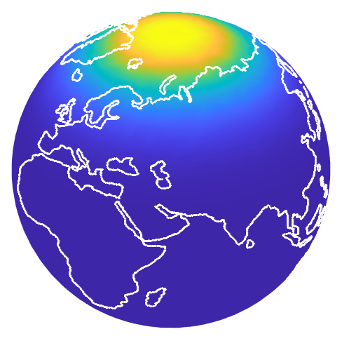
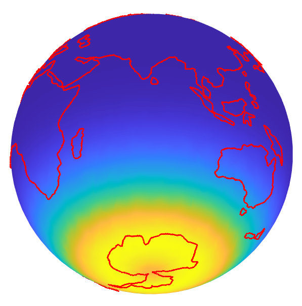
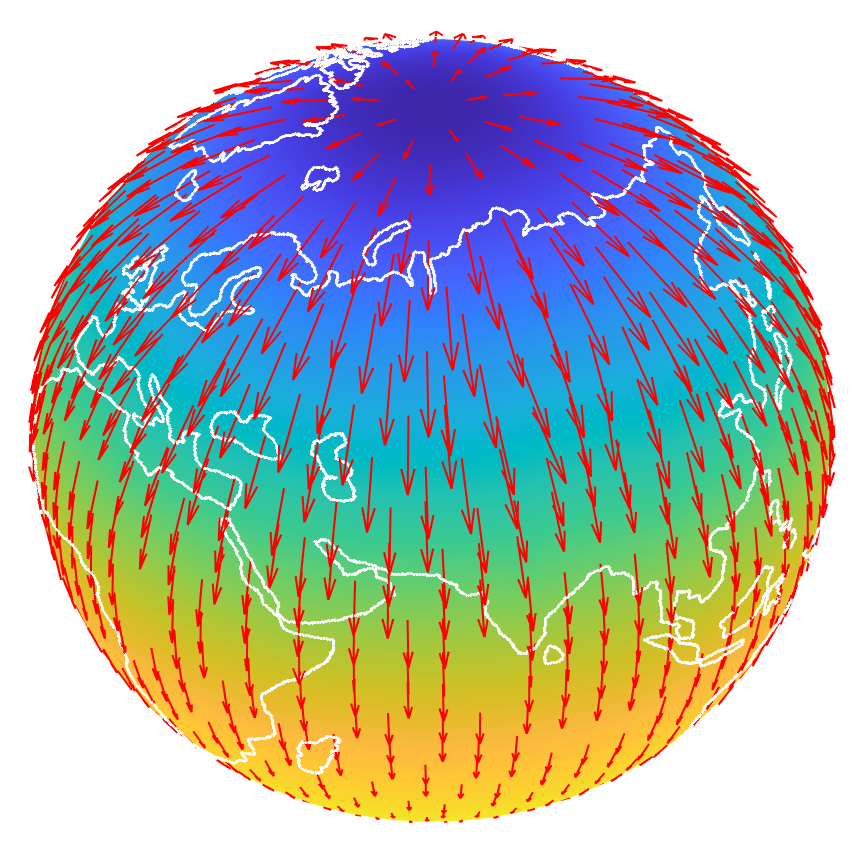
Figure 3. Source density in Figure 3 and target density in Figure 3 and the potential function with the direction of the gradient (red arrows) shown in Figure 3 with an outline of the land masses overlaid to enhance visualization.

Example 2: Peanut Reflector

For this example, we perform a computation with the logarithmic cost $c(\mathbf{x},\mathbf{y})=-\log(1-\mathbf{x}\cdot\mathbf{y})$ arising in the reflector antenna problem. In the reflector antenna problem, we use the potential function $u_{\epsilon}$ to construct the shape of a reflector $\rho$ via the expression:

(61) $$\rho=\mathbf{z}e^{-u_{\epsilon}(\mathbf{z})},\ \ \ \mathbf{z}\in\mathbb{S}^{2}.$$

Note that the reflector is a sphere only when $u_{\epsilon}$ is constant. This case only occurs when $f=g$. In the reflector antenna problem, light originates at the origin (center of the sphere) with a given directional light intensity pattern $f(\mathbf{x})$. Light then travels from the origin and reflects off a reflector with shape given in Equation (61), and then travels in a direction $\mathbf{m}(\mathbf{x})$ to yield a far-field intensity pattern $g(\mathbf{m}(\mathbf{x}))$. Conservation of light intensity, laws of reflection, and a change of variables allow one to solve for the reflector shape via the function $u$ in Equation (61) by solving for $u$ in the Optimal Transport PDE in Equations (7) and (8) with the logarithmic cost $c(\mathbf{x},\mathbf{y})=-\log(1-\mathbf{x}\cdot\mathbf{y})$.

Strictly speaking, a reflector antenna should only be a hemisphere, since the intention is to redirect directional light intensity from the origin (inside the reflector) to the far-field outside the reflector. In order to do this, light must escape, and so the reflector cannot entirely envelop the origin. Temporarily putting physical realities aside, we compute the shape of the reflector for light intensity functions $f$ and $g$ with support equal to $\mathbb{S}^{2}$, demonstrating that the computation can be done for the entire sphere for the cost function $c(\mathbf{x},\mathbf{y})=-\log(1-\mathbf{x}\cdot\mathbf{y})$. We use a source density function which resembles a headlights of a car projected onto a sphere and a constant target density. The densities and the resulting “peanut-shaped” reflector is shown in Figure 4. This computation was inspired by the work in [30] and was also done in [13].

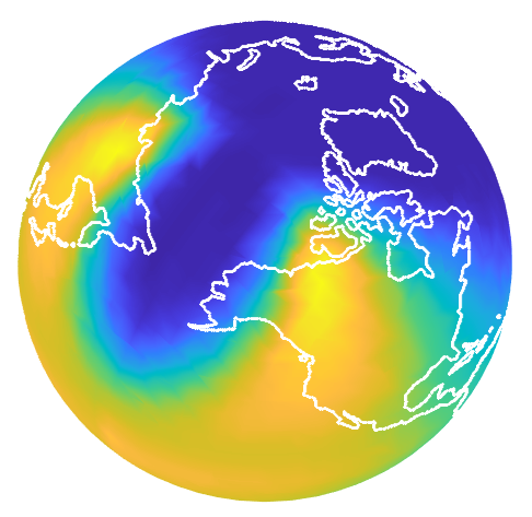
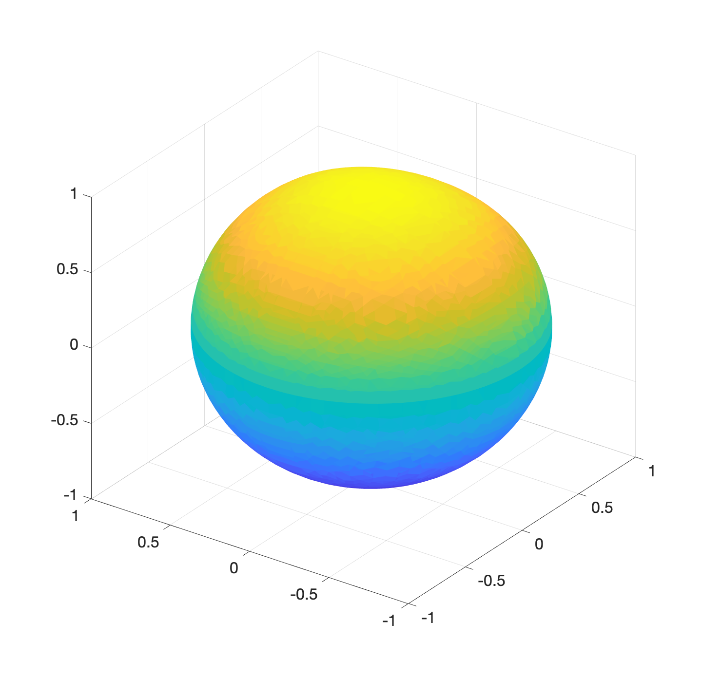
Figure 4. Source density in Figure 4 and target density in Figure 4 and the resulting reflector shape. Note that the reflector is not a sphere, but rather the shape given in Equation (61).

Example 3: Non-Lipschitz Target Density

For this example, we have chosen $\epsilon=0.2$ and $h=0.1$ performed the computation on a grid of $5038$ points. We perform the computation for the squared geodesic cost function $c(\mathbf{x},\mathbf{y})=\frac{1}{2}d_{\mathbb{S}^{2}}(\mathbf{x},\mathbf{y})^{2}$ and for the following source and target density functions for Cartesian coordinates $(x,y,z)$:

$$f(x,y,z) =(1-\epsilon_{5})\frac{1}{\alpha_{7}}e^{-5\arccos{x}^{2}}+\frac{\epsilon_{5}}{4\pi},$$

$$g(x,y,z) =(1-\epsilon_{6})/2\pi, \text{if}\ z\geq 0$$

$$g(x,y,z) =\epsilon_{6}/4\pi, \text{otherwise},$$

where $\epsilon_{5}=0.3$, $\epsilon_{6}=0.1$ and $\alpha_{7}=0.607788$ and the extended density functions are given by Equation (18). The target mass density in this example is discontinuous and equal to zero over half the sphere. This is an important and difficult test example since the target density, while bounded away from zero, is not Lipschitz because it is discontinuous. Figure 5 shows the source and target densities and the resulting quiver plot of the direction of the gradient of the potential function.

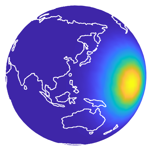
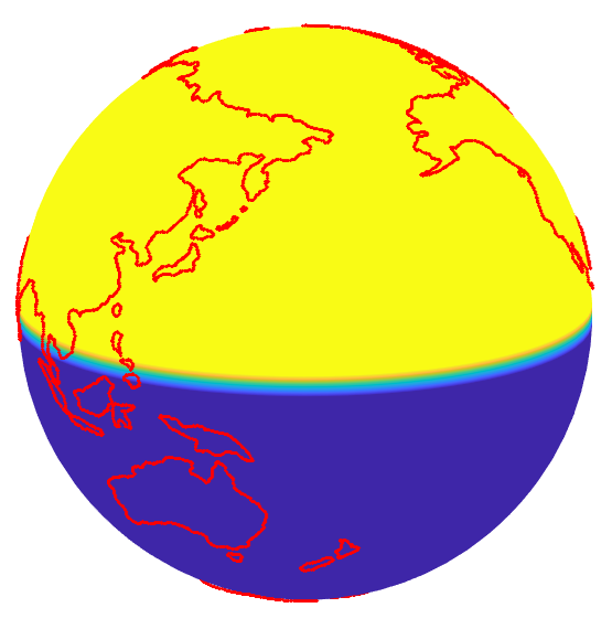
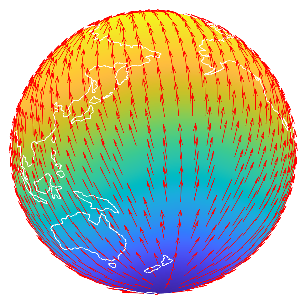
Figure 5. Source density shown in Figure 5, target density in Figure 5 and the potential function with its gradient (red arrows) showing mass moving from the middle of the Pacific Ocean to the northern hemisphere in Figure 5

We have source mass concentrated in the middle of the Pacific Ocean being transported to constant mass density covering the northern hemisphere (note that the maximum values shown in Figure 5 may be the same shade of yellow, but the actual values for the maximum of the density function for the source mass is much higher than the target density). Equation (46) tells us that the gradient of the potential function around where the source mass is concentrated (middle of the Pacific Ocean) should be pointing to the northern hemisphere, so the mass gets appropriately spread out. This is, in fact, what we see from Figure 5.

Example 4: Constant Solution

In the case that the source density function equals the target density function $f=g$, the solution to the Optimal Transport problem on the sphere is given by the potential function $u=\text{constant}$ or $m(x)=x$, for any appropriate cost function. We test our scheme for squared geodesic cost function $c(\mathbf{x},\mathbf{y})=\frac{1}{2}d_{\mathbb{S}^{2}}(\mathbf{x},\mathbf{y})^{2}$. Note, again, that all computations are performed on $T_{\epsilon}$, and thus, for this example we give the formulas for $f_{\epsilon}$ and $g_{\epsilon}$:

(62) $$f_{\epsilon}(x,y,z)=g_{\epsilon}(x,y,z)=\frac{x^{2}+y^{2}+z^{2}}{8\epsilon\pi}.$$

We emphasize that these densities are not constant in $T_{\epsilon}$, however they are derived from constant densities defined on the unit sphere $f=g=1/4\pi$. Even though these densities are not constant, the computed potential function is very close to being constant. For $\epsilon=0.2$ and $h=0.1$, we have computed a solution $u$ which satisfies $\left|\max_{i}u(x_{i})-\min_{i}u(x_{i})\right|=0.000563$, see Figure 6.

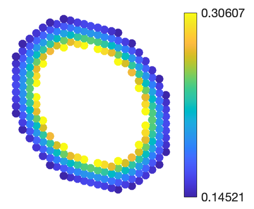
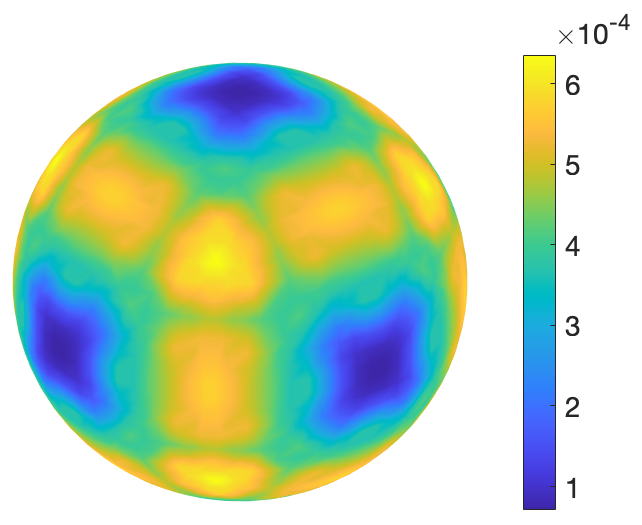
Figure 6. A vertical cross section of the densities $f_{\epsilon},g_{\epsilon}$ in Figure 6 and the resulting solution $u$, which is approximately constant in Figure 6

4.2.1. Studies with Varying $\sigma$, $\epsilon$, and $h$

Fixing $\sigma=1$, we demonstrate that changing the width of the tubular neighborhood does not change the computed solution. The computation is performed using the source and target densities

$$f(x,y,z) =(1-\epsilon_{2})\left(\frac{1}{2\alpha_{1}}e^{-4(\arccos{z}-\frac{1}{2})^{2}}+\frac{1}{2\alpha_{2}}e^{-4(\arccos(y)-\frac{5}{2})^{2}}\right)+\frac{\epsilon_{2}}{4\pi},$$

$$g(x,y,z) =(1-\epsilon_{2})\left(\frac{1}{2\alpha_{3}}e^{-4(\arccos{x}-\pi+\frac{9}{10})^{2}}+\frac{1}{2\alpha_{4}}e^{-4(\arccos(z)-\frac{7}{10})^{2}}\right)+\frac{\epsilon_{2}}{4\pi}.$$

where $\epsilon_{2}=0.2$, $\alpha_{1}=2.57656$, $\alpha_{2}=3.15727$, $\alpha_{3}=4.10094$ $\alpha_{4}=3.38728$ and whose extended densities are given by Equation (18). In Figure 7, we show the potential functions $u$ by varying $\epsilon$ and $h$. The difference in the two solutions has an approximate computed $L^{\infty}$ norm of $0.0059$. The error is computed by interpolating both solutions onto the unit sphere in order to directly compare the values. The grid with $\epsilon=0.2$ and $h=0.1$ has $5038$ points and the grid with $\epsilon=0.1$ and $h=0.05$ has $20068$ points.

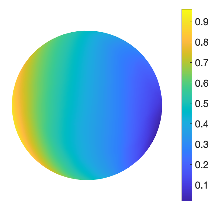
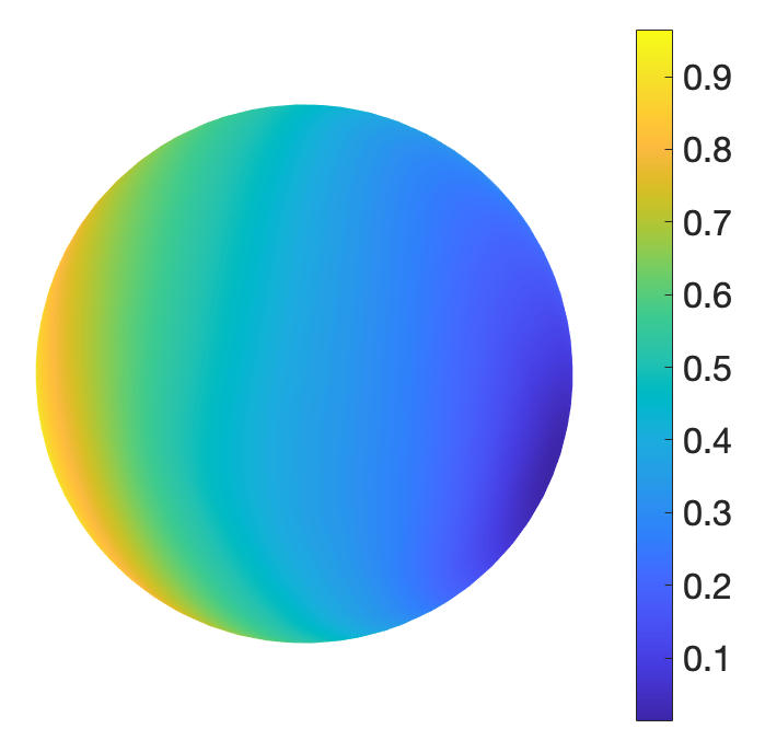
Figure 7. The potential function for $\epsilon=0.2$ and $h=0.1$ in Figure 7 and for $\epsilon=0.1$ and $h=0.05$ in Figure 7

In our second study, we examine the convergence of the residual when we change $\epsilon$ and $h$. Setting $\sigma=1$, we compare the convergence rate of the residual to tolerance $0.1$ for a test using $\epsilon=0.2$ and $h=0.1$ and another test using $\epsilon=0.1$ and $h=0.05$ and the result is shown in Figure 8. The number of iterations to the same tolerance are very similar, showing that Algorithm 1 is not sensitive, in terms of number of iterations, to changes in $h$ and $\epsilon$, as desired. Naturally, the test using $\epsilon=0.1$ and $h=0.05$ has more computational points, so each iteration takes longer.

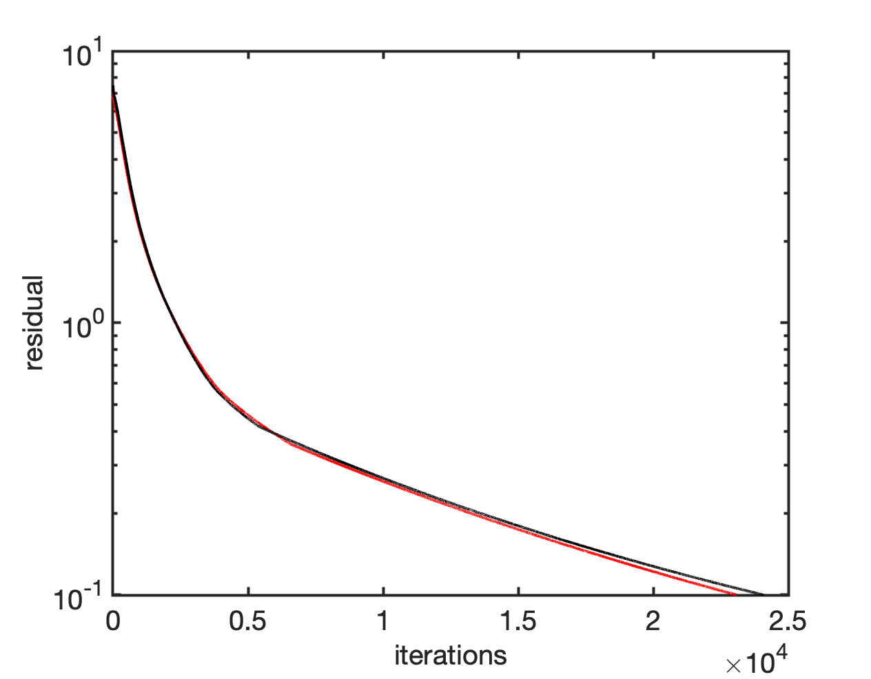
Figure 8. The convergence of the residual for $\epsilon=0.2$ and $h=0.1$ shown in black and $\epsilon=0.1$ and $h=0.05$ shown in red for Algorithm 1.

In our third study, we examine what happens when we vary $\sigma$, the penalty parameter. The results seem to indicate that above a certain threshold, the choice of $\sigma$ does not change the computed solution. The following table shows the maximum absolute difference between the potential function computed with different values for $\sigma$ for $\epsilon=0.2$ and $h=0.1$. Values on the diagonal of the table above are either redundant or uninformative and thus are omitted.

$\sigma$	0.25	0.5	1	2	4	8	16
$0.25$	-	-	-	-	-	-	-
$0.5$	0.1569	-	-	-	-	-	-
$1$	0.2729	0.1160	-	-	-	-	-
$2$	0.3502	0.1934	0.0774	-	-	-	-
$4$	0.3939	0.2371	0.1211	0.0437	-	-	-
$8$	0.4097	0.2529	0.1370	0.0597	0.0168	-	-
$16$	0.4028	0.2450	0.1293	0.0542	0.0199	0.0085	-

4.2.2. Effect of $\epsilon$ and $h$ on Condition Number

In our first study of varying $\epsilon$ and $h$, we approximately fix the number of interior points $N_{I}$ and vary the value of $\epsilon$ and $h$. With a fixed time-step $\Delta t=0.000025$, we find that the number of iterations $k$ required to reach a residual tolerance of $1$ is approximately constant.

$N_{I}$	$\epsilon$	$h$	$k$
$10552$	$0.1$	$0.046$	$2335$
$10424$	$0.15$	$0.057$	$2556$
$10516$	$0.2$	$0.065$	$2588$
$10698$	$0.25$	$0.072$	$2598$
$10320$	$0.3$	$0.079$	$2615$

In our second study, we fix $h$ and change $\epsilon$, while using the same step size $\Delta t=0.000025$ and record the number of iterations $k$ required to reach a residual tolerance of $1$. Again, we observe that the number of iterations does not vary much until $N_{I}$ becomes too small.

$N_{I}$	$\epsilon$	$h$	$k$
$31658$	$0.22$	$0.05$	$2667$
$19162$	$0.16$	$0.05$	$2623$
$11134$	$0.12$	$0.05$	$2470$
$7550$	$0.102$	$0.05$	$2178$

5. Conclusion

In this article, we have extended the Optimal Transport problem on a compact 2D surface $\Gamma\subset\mathbb{R}^{3}$ onto a thin tubular neighborhood $T_{\epsilon}$ with width $\epsilon$. We showed how one can then compute the Optimal Transport mapping $\mathbf{m}$ for the Optimal Transport problem on $\Gamma$ by solving instead for the Optimal Transport mapping $\mathbf{m}_{\epsilon}$ which is the solution to the extended Optimal Transport problem on $T_{\epsilon}$. The key is to extend the density functions and cost function in an appropriate way. The primary benefit of this extension is that the PDE formulation of the Optimal Transport problem on $T_{\epsilon}$ has only Euclidean derivatives. This allows us the flexibility to design a discretization that uses a Cartesian grid. We have discretized the extended PDE formulation of the Optimal Transport problem on $T_{\epsilon}$ and shown its ease of implementation and success with various computational examples on the sphere, some of which are very challenging with other currently available methods.

References

- [1] G. Barles and P. E. Souganidis. Convergence of approximation schemes for fully nonlinear second order equations. Asymptotic Analysis, 4:271–283, 1991.
- [2] M. Bauer, S. Joshi, and K. Modin. Diffeomorphic density matching by optimal information transport. Society for Industrial and Applied Mathematics Journal on Imaging Sciences, 8(3):1718–1751, 2015.
- [3] K. Brix, Y. Hafizogullari, and A. Platen. Designing illumination lenses and mirrors by the numerical solution of Monge-Ampère equations. Journal of the Optical Society of America A, 32(11):2227–2236, 2015.
- [4] J. Chu and R. Tsai. Volumetric variational principles for a class of partial differential equations defined on surfaces and curves. Res Math Sci, 5(19), 2018.
- [5] M. Cuturi. Sinkhorn distances: Lightspeed computation of optimal transportation distances. Advances in Neural Information Processing Systems, 26, June 2013.
- [6] L. L. Doskolovich, D. A. Bykov, A. A. Mingazov, and E. A. Bezus. Optimal mass transportation and linear assignment problems in the design of freeform refractive optical elements generating far-field irradiance distributions. Optics Express, 27(9):13083–13097, 2019.
- [7] H. Federer. Curvature measures. Transactions of the American Mathematical Society, (93):418–491, 1959.
- [8] A. Figalli, L. Rifford, and C. Villani. On the Ma-Trudinger-Wang curvature on surfaces. Calculus of Variations, 39:307–332, 2010.
- [9] T. Glimm and V. Oliker. Optical design of single reflector systems and the Monge-Kantorovich mass transfer problem. Journal of Mathematical Sciences, 117(3):4096–4108, 2003.
- [10] B. D. Hamfeldt. Convergence framework for the second boundary value problem for the Monge-Ampère equation. Society for Industrial and Applied Mathematics Journal on Numerical Analysis, 57(2):945–971, January 2019.
- [11] B. F. Hamfeldt and J. Lesniewski. Convergent finite difference methods for fully nonlinear elliptic equations in three dimensions. Journal of Scientific Computing, 90(35), March 2022.
- [12] B. F. Hamfeldt and A. G. R. Turnquist. A convergent finite difference method for optimal transport on the sphere. Journal of Computational Physics, 445, November 2021.
- [13] B. F. Hamfeldt and A. G. R. Turnquist. Convergent numerical method for the reflector antenna problem via optimal transport on the sphere. Journal of the Optical Society of America A, 38:1704–1713, 2021.
- [14] B. F. Hamfeldt and A. G. R. Turnquist. A convergence framework for optimal transport on the sphere. Numerische Mathematik, 151:627–657, June 2022.
- [15] C. Kublik and R. Tsai. Integration over curves and surfaces defined by the closest point mapping. Research in the mathematical sciences, 3(3), 2016.
- [16] H. Lavenant, S. Claici, E. Chien, and J. Solomon. Dynamic optimal transport on discrete surfaces. ACM Transactions on Graphics (SIGGRAPH Asia 2018), 37(6), December 2018.
- [17] J. Liang and H. Zhao. Solving partial differential equations on point clouds. SIAM Journal on Scientific Computing, 35(3), May 2013.
- [18] G. Loeper. On the regularity of solutions of optimal transportation problems. Acta Mathematica, 202:241–283, 2009.
- [19] G. Loeper. Regularity of optimal maps on the sphere: the quadratic cost and the reflector antenna. Archive for rational mechanics and analysis, 199(1):269–289, 2011.
- [20] X.-N. Ma, N. X. Trudinger, and X.-J. Wang. Regularity of potential functions of the optimal transportation problem. Archive for Rational Mechanics and Analysis, 177(2):151–183, 2005.
- [21] C. B. Macdonald and S. J. Ruuth. The implicit closest point method for the numerical solution of partial differential equations on surfaces. SIAM Journal on Scientific Computing, 31(6):4330–4350, 2010.
- [22] L. Martin and Y.-H. R. Tsai. Equivalent extensions of Hamilton–Jacobi–Bellman equations on hypersurfaces. Journal of Scientific Computing, 84(3):43, 2020.
- [23] R. J. McCann. Polar factorization of maps on Riemannian manifolds. Geometric and Functional Analysis, 11:589–608, 2001.
- [24] M. Neilan. A unified analysis of three finite element methods for the Monge-Ampère equation. Electronic Transactions on Numerical Analysis, 41:262–288, 2014.
- [25] Y. Nesterov. A method of solving a convex programming problem with convergence rate . Soviet Mathematics Doklady, 27:372–376, 1983.
- [26] A. M. Oberman. Convergent difference schemes for degenerate elliptic and parabolic equations: Hamilton–Jacobi equations and free boundary problems. Society for Industrial and Applied Mathematics Journal on Numerical Analysis, 44(2):879–895, 2006.
- [27] V. Oliker. Freeform optical systems with prescribed irradiance properties in near-field. In International Optical Design Conference 2006, volume 6342, page 634211, California, United States, 2006. International Society for Optics and Photonics.
- [28] V. Oliker, J. Rubinstein, and G. Wolansky. Supporting quadric method in optical design of freeform lenses for illumination control of a collimated light. Advances in Applied Mathematics, 62:160–183, 2015.
- [29] L. B. Romijn. Generated Jacobian Equations in Freeform Optical Design: Mathematical Theory and Numerics. PhD thesis, Eindhoven University of Technology, 2021.
- [30] L. B. Romijn, J. H. M. ten Thije Boonkkamp, and W. L. IJzerman. Inverse reflector design for a point source and far-field target. Journal of Computational Physics, 408:109283, 2020.
- [31] S. Ruuth and B. Merriman. A simple embedding method for solving partial differential equations on surfaces. Journal of Computational Physics, 227(3):1943–1961, 2008.
- [32] F. Santambrogio. Optimal Transport for Applied Mathematicians, volume 55. Birkhäuser, Basel, Switzerland, 2015.
- [33] H. Schaeffer and T. Y. Hou. An accelerated method for nonlinear elliptic PDE. Journal of Scientific Computing, 69(2):556–580, 2016.
- [34] J. Solomon, R. Rustamov, L. Guibas, and A. Butscher. Earth mover’s distances on discrete surfaces. Association for Computing Machinery Transactions on Graphics, 33(4):1–12, July 2014.
- [35] J. Urbas. On the second boundary value problem for equations of Monge-Ampère type. Journal für die reine und angewandte Mathematik, 487:115–124, 1997.
- [36] X.-J. Wang. On the design of a reflector antenna. IOP Science, 12:351–375, 1996.
- [37] X.-J. Wang. On the design of a reflector antenna II. Calculus of Variations and Partial Differential Equations, 20(3):329–341, 2004.
- [38] H. Weller, P. Browne, C. Budd, and M. Cullen. Mesh adaptation on the sphere using optimal transport and the numerical solution of a Monge-Ampère type equation. Journal of Computational Physics, 308:102–123, 2016.
- [39] R. Wu, L. Xu, P. Liu, Y. Zhang, Z. Zheng, H. Li, and X. Liu. Freeform illumination design: a nonlinear boundary problem for the elliptic Monge-Ampére equation. Optics Letters, 38(2):229–231, 2013.
- [40] N. K. Yadav. Monge-Ampère Problems with Non-Quadratic Cost Function: Application to Freeform Optics. PhD thesis, Technische Universiteit Eindhoven, Eindhoven, Netherlands, 2018.
- [41] J. Yu, R. Lai, W. Li, and S. Osher. Computational mean-field games on manifolds. Journal of Computational Physics, 484(112070), July 2023.