Copyright
by
Author Name Required !!!
2023
The Dissertation Committee for Author Name Required !!!
certifies that this is the approved version of the following dissertation:
Title Required !!!
Committee:
Per-Gunnar Martinsson, Supervisor
Rachel Ward, Co-supervisor
Joseph Kileel
George Biros
Yuji Nakatsukasa
Acknowledgments
\@afterheading
Words are insufficient to convey my appreciation to my advisors, Prof. Per-Gunnar Martinsson and Prof. Rachel Ward, for their guidance and support throughout my Ph.D. journey. Their knowledge and insights have been lighthouses that navigate me in the fascinating realms of numerical linear algebra and machine learning. They have provided invaluable advice for both my research and my career, beyond the scope of this thesis. They endow me with the horizon to broaden my view and explore different research areas. Their passion and devotion to research encourage me to follow and try pursuing an academic career.
In addition to my advisors, I have had the fortune to collaborate with and learn from some great applied mathematicians and computer scientists during my doctoral research, including Shuo Yang, Prof. Sujay Sanghavi, Prof. Inderjit Dhillon, Prof. Qi Lei, Yuege Xie, Prof. Yuji Nakatsukasa, Kevin Miller, Kate Pearce, and Chao Chen. Works presented in this thesis and beyond could not have been finished without their efforts. More importantly, their meticulousness and diligence motivate me as a researcher; while their erudition helps diversify my sight from various aspects.
In particular, I would like to give my profound thanks to Prof. Qi Lei, who has been an inspiring mentor, as well as a supportive friend, since the beginning of my graduate study, who introduced me to the splendid field of statistical learning theory, and who constantly influences me with her vision and attitude towards research.
Meanwhile, I am sincerely grateful for the constructive suggestions and generous help of Prof. Joseph Kileel, Prof. George Biros, and Prof. Yuji Nakatsukasa, together with my advisors, who kindly serve on my thesis committee. Especially, I would like to thank Prof. Yuji Nakatsukasa for the insightful discussions and guidance on several projects in numerical linear algebra.
I truly appreciate the experience in Prof. Martinsson’s and Prof. Ward’s research groups, both of which involve brilliant researchers and collaborative environments where I have learned millions. I am thankful to everyone in both groups, especially my collaborators among them: Yuege Xie, Kevin Miller, Kate Pearce, and Chao Chen; along with Anna Yesypenko, Ke Chen, Bowei Wu, Heather Wilber, Ruhui Jin, Amelia Henriksen, Xiaoxia Wu, and more for their enlightening advice at different stages of my graduate study. It is also my fortune to be a part of the broader Oden community, learning from its incredible variety of research directions while enjoying its inclusiveness.
Despite the fleeting time, my four years as an undergraduate student at Emory University before graduate school were irreplaceable for my professional and personal development. Looking back, I am genuinely grateful to my undergraduate advisors Prof. Effrosyni Seitaridou and Prof. Eric Weeks for patiently unveiling a corner of the research world to a curious undergraduate, as well as for encouraging me to follow my interests while pursuing doctoral study along a different direction. I was also fortunate enough to make some cherished friendships during my undergraduate, among which I am truly thankful to Xiaoyi Zhang whose wisdom and attitude on life have always inspired and motivated me since our paths first crossed.
Finally, I would like to give my wholehearted gratitude to my parents. I owe them for being mostly away from home in the past nine years and probably more years to come, for the absence during their struggles in the COVID-19 pandemic, and everything. Their unconditional love and support have never been diminished by distance.
Title Required !!!
by
Author Name Required !!!, Ph.D.
The University of Texas at Austin, 2023
Supervisors: Per-Gunnar Martinsson
Rachel Ward
Large models and enormous data are essential driving forces of the unprecedented successes achieved by modern algorithms, especially in scientific computing and machine learning. Nevertheless, the growing dimensionality and model complexity, as well as the non-negligible workload of data pre-processing, also bring formidable costs to such successes in both computation and data aggregation. As the deceleration of Moore’s Law slackens the cost reduction of computation from the hardware level, fast heuristics for expensive classical routines and efficient algorithms for exploiting limited data are increasingly indispensable for pushing the limit of algorithm potency. This thesis explores some of such algorithms for fast execution and efficient data utilization.
-
1.
From the computational efficiency perspective, we design and analyze fast randomized low-rank decomposition algorithms for large matrices based on “matrix sketching”, which can be regarded as a dimension reduction strategy in the data space. These include the randomized pivoting-based interpolative and CUR decomposition discussed in Chapter 2 and the randomized subspace approximations discussed in Chapter 3.
-
2.
From the sample efficiency perspective, we focus on learning algorithms with various incorporations of data augmentation that improve generalization and distributional robustness provably. Specifically, Chapter 4 presents a sample complexity analysis for data augmentation consistency regularization where we view sample efficiency from the lens of dimension reduction in the function space. Then in Chapter 5, we introduce an adaptively weighted data augmentation consistency regularization algorithm for distributionally robust optimization with applications in medical image segmentation.
Table of Contents
\@afterheading
\@starttoctoc
List of Tables
\@afterheading
\@starttoclot
List of Figures
\@afterheading
\@starttoclof
\nobibliography*
Chapter 1 Overview
1.1 Computational Efficiency: Randomized Low-rank Decompositions
Low-rank decompositions are dimension reduction techniques that unveil latent low-dimensional structures in large matrices, which are ubiquitous in various applications like principal component analysis and spectral clustering. However, to compute common matrix decompositions (e.g., SVD) of an matrix, classical deterministic algorithms generally scale as , making them untenable for large-scale problems.
As a remedy, the “matrix sketching” framework [68] embeds high-dimensional matrices into random low-dimensional subspaces via fast linear transforms, commonly known as randomized linear embeddings or (fast) Johnson-Lindenstrauss transforms. Some popular choices include Gaussian random matrices [78], subsampled random trigonometric transforms [166], and sparse embeddings like count sketch [103] and sparse sign matrices [30]. After such dimension reduction through randomized linear embedding, classical matrix decomposition algorithms can be executed efficiently, and low-rank approximations can be reconstructed without much compromise in accuracy.
Chapter 2 and Chapter 3 of this thesis explore the potency of randomization with “matrix sketching” in two classical low-rank decomposition problems, namely the matrix skeletonization and the randomized subspace approximation.
1.1.1 Randomized Pivoting-based Matrix Skeletonization
Given a matrix , the matrix skeletonization problem (i.e., interpolative decomposition (ID) and CUR decomposition) solves for low-rank “natural bases” formed by the original columns (and/or rows) of . Precisely, the goal is to identify column (or row) skeletons (or , in MATLAB notation) indexed by (or where ) that serve as good bases,
Despite the NP-hardness [29] of identifying the nearly optimal skeleton selections like the row/column subset with the maximum spanning volume [61], there exists fast heuristics [96, 137, 153, 40] that enjoys statistical guarantees and/or practical successes. In particular, randomization via “matrix sketching” plays a critical role in many of these heuristics [153, 25, 45].
Randomized pivoting-based matrix skeletonization [137, 153, 45] is a class of such fast heuristics widely used in scientific computing, whose general framework consists of two stages:
-
(i)
dimension reduction via sketching (e.g., constructing row sketch via a Gaussian random matrix with i.i.d. entries and ) and
-
(ii)
greedy skeleton selection via pivoting on the reduced matrix sketch (e.g., applying LU with partial pivoting on and taking the first pivots as the column skeletonizations).
In Chapter 2, we first surveyed and compared different options for the two stages, e.g., sketching/randomized SVD [68] for the dimension reduction stage and column pivoted QR (CPQR)/LU with partial pivoting (LUPP) for the pivoting stage. Motivated by the systematic comparison, we then proposed a novel combination of sketching and LU with partial pivoting (LUPP) for efficient randomized matrix skeletonization. Compared to column pivoted QR (CPQR) commonly used in the existing algorithms, LUPP enjoys superior empirical efficiency and parallelizability [62, 136] while compromising the rank-revealing guarantees. Fortunately, for matrix skeletonization, such a trade-off between efficiency and rank-revealing property can be avoided via sketching. In particular, we demonstrated that, instead of relying on rank-revealing properties of the pivoting scheme, the simple combination of sketching and LUPP exploits the spectrum-preserving capability of sketching and achieves considerable acceleration without compromising accuracy.
1.1.2 Randomized Subspace Approximations
Theoretical underpinnings of randomized subspace approximation is another key aspect of analyzing randomized low-rank decompositions. A low-rank decomposition can be viewed as a bilinear combination of the associated low-rank bases for the column and row spaces that encapsulate key information for a wide range of tasks (e.g., canonical component analysis and leverage score sampling). Specifically, for a truncated SVD
the left and right leading singular vectors and can be approximated efficiently via randomized subspace approximations. In the basic version, randomized subspace approximations leverage the appealing property of randomized linear embeddings (e.g., a Gaussian embedding with i.i.d. entries ) that, with moderate oversampling , sketching (with power iterations) captures the leading singular vectors with high probability. Under orthonormalization at each iteration (commonly known as randomized subspace iteration [68, Algorithm 4.4]), provides a numerical stable estimate for the leading singular subspace.
Canonical angles [59] (formally defined in Definition 3.1) are commonly used to quantify the difference between two subspaces of the same space, which provides natural error measures for the randomized subspace approximations. For instance, given arbitrary full-rank matrices and (assuming without loss of generality), the canonical angles between their corresponding range subspaces in are given by the spectra of where the columns of and consist of orthonormal bases of and , respectively. Precisely, for each , , or equivalently, (cf. [183] Section 3).
In Chapter 3, we extended the existing analysis on the accuracy of singular vectors approximated by the randomized subspace iteration, in terms of the canonical angles between the true and approximated leading singular subspaces and . By casting a computational efficiency view on the bounds and estimates of canonical angles, we provided a set of prior probabilistic bounds that is not only asymptotically tight but also computable in linear time. Moreover, we derived unbiased prior estimates, along with residual-based posterior bounds, of canonical angles that can be evaluated efficiently, while further demonstrating the empirical effectiveness of these bounds and estimates with numerical evidence.
1.2 Sample Efficiency: Data Augmentation for Better Generalization
Modern machine learning models, especially deep learning models, require substantially large amounts of samples for training. However, data collection and human annotation often come with non-negligible costs in practice. Therefore, sample efficiency and generalization are critical properties of learning algorithms. In the most basic setting, a learning algorithm is designed for recovering some unknown ground truths (e.g., descriptions of images) via sampling from some unknown distributions (e.g., images from the Internet with descriptions). The goal is to learn a prediction function (e.g., image captioning) that well approximates the ground truth by providing accurate predictions beyond the training samples (e.g., (in-distribution) generalization to unseen testing samples from the same distribution or out-of-distribution generalization to testing samples from related but different distributions), with as few training samples as possible (i.e., sample efficiency).
Since the seminal work [84], data augmentation has been a ubiquitous ingredient in many state-of-the-art machine learning algorithms [132, 133, 71, 34, 85]. It started from simple transformations on samples (e.g., (random) perturbations, distortions, scales, crops, rotations, and horizontal flips on images) that roughly preserve the semantic information. More sophisticated variants were subsequently designed; a non-exhaustive list includes Mixup [177], Cutout [43], and Cutmix [175]. Despite the known capability of improving generalization and sample efficiency empirically, the theoretical understanding of how data augmentation works remain limited due to the wide variety of domain-specific designs [125, 177] and algorithmic choices of utilizing data augmentations [84, 135, 70]. The classical wisdom interprets and leverages data augmentation as a natural expansion of the original training samples [84, 132, 34, 133, 71]. However, simply enlargening the training set is not sufficient to explain the unprecedented successes (in comparison to the classical wisdom) recently achieved by an alternative line of data-augmentation-based learning algorithms — data augmentation consistency regularization [5, 88, 124, 135, 13] — that encourages similar predictions among the original sample and its augmentations.
Chapter 4 and Chapter 5 of this thesis discuss the sample efficiency of data augmentation consistency regularization from the dimension reduction aspect, along with an application in medical image segmentation.
1.2.1 Sample Efficiency of Data Augmentation Consistency Regularization
In efforts to interpret the effect of different algorithmic choices on utilizing data augmentations, Chapter 4 conducts apple-to-apple comparisons between two popular data-augmentation-based algorithms — the empirical risk minimization on the augmented training set (DA-ERM) and the data augmentation consistency regularization (DAC) — in the supervised setting.
Concretely, given a ground truth distribution and a well-specified function class (e.g., a class of neural networks with a sufficiently expressive hidden-layer representation function ) such that for a given loss function , , let be a set of training samples drawn i.i.d. from and
be the features of its (random) augmentation (i.e., additional augmentations per sample). Considering the basic version of data augmentation which preserves the labels of original samples, DA-ERM directly includes the augmented samples in the training set and learns via empirical risk minimization (ERM),
Instead, DAC regularization rewards that provides similar representations among data augmentations of the same sample,
where is a metric associated with the metric space (e.g., the Euclidean distance).
Previous works [27, 102, 16] generally view augmentations as groups endowed with Haar measures which inevitably assumed access to augmentations over the population. By contrast, we investigate a more realistic circumstance where both the training data and their augmentations are presented as finite random samples, and , by considering the DAC regularization as a reduction in the complexity of the function class (e.g., a dimension reduction in the linear regression setting). Apart from the well-known semi-supervised learning capability of DAC, in Chapter 4, we demonstrated the intrinsic efficiency of DAC over DA-ERM in utilizing both samples and their augmentations, even without unlabeled data, by establishing separations of sample complexities between DAC and DA-ERM in various settings, including different function classes (e.g., linear regression and neural networks), different data augmentations, as well as in-distribution and out-of-distribution generalization.
1.2.2 Adaptively Weighted Data Augmentation Consistency Regularization
Grounding the theoretical insight on data augmentation consistency regularization as guidance for algorithm design, in Chapter 5, we explore the combination of data augmentation consistency regularization and sample reweighting for a distributionally robust optimization setting commonly encountered in medical image segmentation.
Concept shift is a prevailing problem in natural tasks like medical image segmentation where samples usually come from different subpopulations with variant correlations between features and labels. A common type of concept shift in medical image segmentation is the “information imbalance” between the label-sparse samples with few (if any) segmentation labels and the label-dense ones with plentiful labeled pixels. Existing distributionally robust algorithms have focused on adaptively truncating/down-weighting the “less informative” (i.e., label-sparse) samples. To exploit data features of label-sparse samples more efficiently, in Chapter 5, we propose an adaptively weighted online optimization algorithm — AdaWAC— to incorporate data augmentation consistency regularization in sample reweighting. As a simplified overview, when learning from a function class parameterized by , AdaWAC introduces a set of trainable weights to balance the supervised (cross-entropy) loss and unsupervised consistency regularization 111Here, and denote the (random) augmentations associated with for each (refer to Section 5.2 for formal definitions). of each sample separately:
At the saddle point of the underlying objective, the weights assign label-dense samples to the supervised loss (i.e., ) and label-sparse samples to the unsupervised consistency regularization (i.e., ). We provide a convergence guarantee by recasting the optimization as online mirror descent on a saddle point problem. Our empirical results further demonstrate that AdaWAC not only enhances the segmentation performance and sample efficiency but also improves the robustness to concept shift on various medical image segmentation tasks with different UNet-style backbones.
Chapter 2 Randomized Pivoting Algorithms for CUR and Interpolative Decompositions
Abstract
Matrix skeletonizations like the interpolative and CUR decompositions provide a framework for low-rank approximation in which subsets of a given matrix’s columns and/or rows are selected to form approximate spanning sets for its column and/or row space.
Such decompositions that rely on “natural” bases have several advantages over traditional low-rank decompositions with orthonormal bases, including preserving properties like sparsity or non-negativity, maintaining semantic information in data, and reducing storage requirements.
Matrix skeletonizations can be computed using classical deterministic algorithms such as column-pivoted QR, which work well for small-scale problems in practice, but suffer from slow execution as the dimension increases and can be vulnerable to adversarial inputs.
More recently, randomized pivoting schemes have attracted much attention, as they have proven capable of accelerating practical speed, scale well with dimensionality, and sometimes also lead to better theoretical guarantees.
This manuscript provides a comparative study of various randomized pivoting-based matrix skeletonization algorithms that leverage classical pivoting schemes as building blocks.
We propose a general framework that encapsulates the common structure of these randomized pivoting-based algorithms and provides an a-posteriori-estimable error bound for the framework. Additionally, we propose a novel concretization of the general framework and numerically demonstrate its superior empirical efficiency.111This chapter is based on the following published journal paper:
\bibentrydong2021simpler [45].
2.1 Introduction
The problem of computing a low-rank approximation to a matrix is a classical one that has drawn increasing attention due to its importance in the analysis of large data sets. At the core of low-rank matrix approximation is the task of constructing bases that approximately span the column and/or row spaces of a given matrix. This manuscript investigates algorithms for low-rank matrix approximations with “natural bases” of the column and row spaces – bases formed by selecting subsets of the actual columns and rows of the matrix. To be precise, given an matrix and a target rank , we seek to determine an matrix holding of the columns of , and a matrix such that
| (2.1) |
We let denote the index vector of length that identifies the chosen columns, so that, in MATLAB notation,
| (2.2) |
If we additionally identify an index vector that marks a subset of the rows that forms an approximate basis for the row space of , we can then form the “CUR” decomposition
| (2.3) |
where is a matrix, and
| (2.4) |
The decomposition (2.3) is also known as a “matrix skeleton” [61] approximation (hence the subscript “s” for “skeleton” in and ). Matrix decompositions of the form (2.1) or (2.3) possess several compelling properties: (i) Identifying and/or is often helpful in data interpretation. (ii) The decompositions (2.1) and (2.3) preserve important properties of the matrix . For instance, if is sparse/non-negative, then and are also sparse/non-negative. (iii) The decompositions (2.1) and (2.3) are often memory efficient. In particular, when the entries of itself are available, or can inexpensively be computed or retrieved, then once and have been determined, there is no need to store and explicitly.
Deterministic techniques for identifying close-to-optimal index vectors and are well established. Greedy algorithms such as the classical column pivoted QR (CPQR) [59, Sec. 5.4.1], and variations of LU with complete pivoting [144, 83] often work well in practice. There also exist specialized pivoting schemes that come with strong theoretical performance guarantees [65].
While effective for smaller dense matrices, classical techniques based on pivoting become computationally inefficient as the matrix sizes grow. The difficulty is that a global update to the matrix is in general required before the next pivot element can be selected. The situation becomes particularly dire for sparse matrices, as each update tends to create substantial fill-in of zero entries.
To better handle large matrices, and huge sparse matrices in particular, a number of algorithms based on randomized sketching have been proposed in recent years. The idea is to extract a “sketch” of the matrix that is far smaller than the original matrix, yet contains enough information that the index vectors and/or can be determined by using the information in alone. Examples include:
- 1.
-
2.
Leverage score sampling: Again, the procedures start by computing approximations to the dominant left and right singular vectors of through a randomized scheme. Then these approximations are used to compute probability distributions on the row and/or column indices, from which a random subset of columns and/or rows is sampled.
-
3.
Pivoting on a random sketch: With a random matrix drawn from some appropriate distribution, a sketch of is formed via . Then, a classical pivoting strategy such as the CPQR is applied on to identify a spanning set of columns.
The existing literature [4, 25, 31, 39, 40, 49, 51, 65, 96, 137, 153] presents compelling evidence in support of each of these frameworks, in the form of mathematical theory and/or empirical numerical experiments.
The objective of the present manuscript is to organize different strategies and to conduct a systematic comparison, with a focus on their empirical accuracy and efficiency. In particular, we compare different strategies for extracting a random sketch, such as techniques based on Gaussian random matrices [68, 78, 100, 165], random fast transforms [19, 68, 100, 118, 146, 166], and random sparse embeddings [30, 100, 103, 111, 147, 165]. We also compare different pivoting strategies such as pivoted QR [59, 153] versus pivoted LU [25, 137]. Finally, we compare how well sampling-based schemes perform in relation to pivoting-based schemes.
In addition to providing a comparison of existing methods, the manuscript proposes a general framework that encapsulates the common structure shared by some popular randomized pivoting-based algorithms and presents an a-posteriori-estimable error bound for the framework. Moreover, the manuscript introduces a novel concretization of the general framework that is faster in execution than the schemes of [137, 153] while picking equally close-to-optimal skeletons in practice. In its most basic version, our simplified method for finding a subset of columns of works as follows:
Sketching step: Draw from a Gaussian distribution and form .
Pivoting step: Perform a partially pivoted LU decomposition of . Collect the chosen pivot indices in the index vector . (Since partially pivoted LU picks rows of , indicates columns of .)
What is particularly interesting about this process is that while the LU factorization with partial pivoting (LUPP) is not rank revealing for a general matrix , the randomized mixing done in the sketching step makes LUPP excel at picking spanning columns. Furthermore, the randomness introduced by sketching empirically serves as a remedy for the vulnerability of classical pivoting schemes like LUPP to adversarial inputs (e.g., the Kahan matrix [79]). The scheme can be accelerated further by incorporating a structured random embedding . Alternatively, its accuracy can be enhanced by incorporating one of two steps of power iteration when building the sample matrix .
The manuscript is organized as follows: Section 2.2 provides a brief overview of the interpolative and CUR decompositions (Section 2.2.2), along with some essential building blocks of the randomized pivoting algorithms, including randomized linear embeddings (Section 2.2.3), randomized low-rank SVD (Section 2.2.4), and matrix decompositions with pivoting (Section 2.2.5). Section 2.3 reviews existing algorithms for matrix skeletonizations (Section 2.3.1, Section 2.3.2), and introduces a general framework that encapsulates the structures of some randomized pivoting-based algorithms. In Section 2.4, we propose a novel concretization of the general framework, and provide an a-posteriori-estimable bound for the associated low-rank approximation error. With the numerical results in Section 2.5, we first compare the efficiency of various choices for the two building blocks in the general framework: randomized linear embeddings (Section 2.5.1) and matrix decompositions with pivoting (Section 2.5.2). Then, we demonstrate the empirical advantages of the proposed algorithm by investigating the accuracy and efficiency of assorted randomized skeleton selection algorithms for the CUR decomposition (Section 2.5.3).
2.2 Background
We first introduce some closely related low-rank matrix decompositions that rely on “natural” bases, including the CUR decomposition, and the column, row, and two-sided interpolative decompositions (ID) in Section 2.2.2. Section 2.2.3 describes techniques for computing randomized sketches of matrices, based on which Section 2.2.4 discusses the randomized construction of low-rank SVD. Section 2.2.5 describes how these can be used to construct matrix decompositions. While introducing the background, we include proofs of some well-established facts that provide key ideas but are hard to extract from the context of relevant references.
2.2.1 Notation
Let be an arbitrary given matrix of rank , whose SVD is given by
such that for any rank parameter , we denote and as the orthonormal bases of the dimension- leading left and right singular subspaces of , while and as the orthonormal bases of the respective orthogonal complements. The diagonal submatrices consisting of the spectrum, and , follow analogously. We denote as the rank- truncated SVD that minimizes rank- approximation error of [55]. Furthermore, we denote the spectrum of , , as a diagonal matrix, while for each , let be the -th singular value of .
For the QR factorization, given an arbitrary rectangular matrix with full column rank (), let be a full QR factorization of such that and consist of orthonormal bases of the subspace spanned by the columns of and its orthogonal complement. We denote () as a map that identifies an orthonormal basis (not necessarily unique) for , .
We adopt MATLAB notation for matrices throughout this work. Unless specified otherwise (e.g., with subscripts), we use to represent either the spectral norm or the Frobenius norm (i.e., holding simultaneously for both norms).
2.2.2 Interpolative and CUR decompositions
We first recall the definitions of the interpolative and CUR decompositions of a given real matrix . After providing the basic definitions, we discuss first how well it is theoretically possible to do low-rank approximation under the constraint that natural bases must be used. We then briefly describe the further suboptimality incurred by standard algorithms.
Basic definitions
We consider low-rank approximations for with column and/or row subsets as bases. Given an arbitrary linearly independent column subset (), the rank- column ID of with respect to column skeletons can be formulated as,
| (2.5) |
where is the orthogonal projector onto the spanning subspace of column skeletons. Analogously, given any linearly independent row subset (), the rank- column ID of with respect to row skeletons takes the form
| (2.6) |
where is the orthogonal projector onto the span of row skeletons. While with both column and row skeletons, we can construct low-rank approximations for in two forms – the two-sided ID and CUR decomposition: with , let be an invertible two-sided skeleton of such that
| Two-sided ID: | (2.7) | ||||
| CUR decomposition: | (2.8) |
where in the exact arithmetic, since , the two-sided ID is equivalent to the column ID characterized by , i.e., . Nevertheless, the two-sided ID and CUR decomposition differ in both suboptimality and conditioning.
Remark 2.1 (Suboptimality of ID versus CUR).
For any given column and row skeletons and ,
| (2.9) |
Rationale for Remark 2.1.
We observe the simple orthogonal decomposition
where and are orthogonal projectors. With the Frobenius norm,
while with the spectral norm
where
and
∎
Remark 2.2 (Conditioning of ID versus CUR).
The construction of CUR decomposition tends to be more ill-conditioned than that of two-sided ID. Precisely, for properly selected column and row skeletons and , the corresponding skeletons , , and share similar spectrum decay as , which is usually ill-conditioned in the context. In the CUR decomposition, both the bases , and the small matrix in the middle tend to suffer from large condition numbers as that of . In contrast, the only potentially ill-conditioned component in the two-sided ID is (i.e., despite being expressed in and , and in Equation 2.7 are well-conditioned, and can be evaluated without direct inversions).
Remark 2.3 (Stable CUR).
Numerically, the stable construction of a CUR decomposition can be conducted via (unpivoted) QR factorization of and ([3], Algorithm 2): let and be matrices from the QR whose columns form orthonormal bases for and , respectively, then
| (2.10) |
Notion of suboptimality
Both interpolative and CUR decompositions share the common goal of identifying proper column and/or row skeletons for whose column and/or row spaces are well covered by the respective spans of these skeletons. Without loss of generality, we consider the column skeleton selection problem: for a given rank , we aim to find a proper column subset, (, ), such that
| (2.11) |
where common choices of the norm include the spectral norm and Frobenius norm ; is a function with for all , and depends on the choice of ; and we recall that yields the optimal rank- approximation error. Meanwhile, similar low-rank approximation error bounds are desired for the row ID , two-sided ID , and CUR decomposition .
Suboptimality of matrix skeletonization algorithms
The suboptimality of column subset selection, as well as the corresponding ID and CUR decomposition, has been widely studied in a variety of literature.
Specifically, with () being the maximal-volume submatrix in , the corresponding CUR decomposition (called pseudoskeleton component in the original paper) satisfies Equation 2.11 in with [61]. However, it was also pointed out in [61] that skeletons associated with the maximal-volume submatrix are not guaranteed to minimize the low-rank approximation error in Equation 2.11. Moreover, identification of the maximal-volume submatrix is known to be NP-hard [29, 184].
Nevertheless, from the pivoting perspective, the existence of rank- column IDs with can be shown constructively via the strong rank-revealing QR factorization [65], which further provides a polynomial-time relaxation for constructing IDs with . From the sampling perspective, the existence of a rank- column ID with for and for can be shown by upper bounding the expectation of for volume sampling [42]. Later on, polynomial-time algorithms were proposed for selecting such column skeletons [41, 33].
2.2.3 Randomized linear embeddings
For a given matrix of rank (typically we consider ), and a distortion parameter , a linear map (i.e., , typically we consider for embeddings) is called an linear embedding of with distortion if
| (2.12) |
A distribution over linear maps (or equivalently, over ) generates randomized oblivious linear embeddings (abbreviated as randomized linear embeddings) if over , Equation 2.12 holds for all with at least constant probability. Given and a randomized linear embedding , provides a (row) sketch of , and the process of forming is known as sketching [165, 100].
Randomized linear embeddings are closely related to various concepts like the Johnson-Lindenstrauss lemma and the restricted isometry property, and are studied in a broad scope of literature. Some popular randomized linear embeddings (cf. [100] Section 8, 9) include:
- 1.
-
2.
subsampled randomized trigonometric transforms (SRTT):
where is a uniformly random selection of out of rows; is an unitary trigonometric transform (e.g., discrete Hartley transform for , and discrete Fourier transform for ); with i.i.d. Rademacher random variables flips signs randomly; and is a random permutation [166, 68, 118, 146, 19, 100]; and
- 3.
Table 2.1 summarizes lower bounds on s that provide theoretical guarantee for Equation 2.12, along with asymptotic complexities of sketching, denoted as , for these randomized linear embeddings. In spite of the weaker guarantees for structured randomized embeddings (i.e., SRTTs and sparse sign matrices) in the theory by a logarithmic factor, from the empirical perspective, is usually sufficient for all the embeddings in Table 2.1 when considering tasks such as constructing randomized rangefinders (which we subsequently leverage for fast skeleton selection). For instance, it was suggested in [68, 100] to take (e.g., ) for Gaussian embeddings, for SRTTs, and , for sparse sign matrices in practice [148].
| Randomized linear embedding | Theoretical best dimension reduction | |
|---|---|---|
| Gaussian embedding | ||
| SRTT | ||
| Sparse sign matrix | , |
2.2.4 Randomized rangefinder and low-rank SVD
Given , the randomized rangefinder problem aims to construct a matrix such that the row space of aligns well with the leading right singular subspace of [100]: is sufficiently small for some unitary invariant norm (e.g., or ). When admits full row rank, we call a rank- row basis approximator of . The well-known optimality result from [55] demonstrated that, for a fixed rank , the optimal rank- row basis approximator of is given by its leading right singular vectors: .
A row sketch generated by some proper randomized linear embedding is known to serve as a good solution for the randomized rangefinder problem with high probability. For instance, with the Gaussian embedding, a small constant oversampling is sufficient for a good approximation [68]:
| (2.13) |
and moreover, with high probability. Similar guarantees hold for spectral norm ([68], Section 10). The randomized rangefinder error depends on the spectral decay of , and can be aggravated by a flat spectrum. In this scenario, power iterations (with proper orthogonalization, [68]), as well as Krylov and block Krylov subspace iterations ([108]), may be incorporated after the initial sketching as a remedy. For example, with a randomized linear embedding of size , a row basis approximator with power iterations () is given by
| (2.14) |
and takes takes operations to construct. However, such plain power iteration in Equation 2.14 is numerically unstable and can lead to large errors when is ill-conditioned and . For a stable construction, orthogonalization can be applied at each iteration:
| (2.15) |
with an additional cost of overall.
In addition, with a proper that does not exceed the exact rank of , the row sketch has a full row rank almost surely. Precisely, recall from Section 2.2.1:
Remark 2.4.
For a Gaussian embedding with i.i.d. entries from and , the row sketch has full row rank almost surely.
Rationale for Remark 2.4.
Recall the reduced SVD of , . Given , it is sufficient to show that . Since consists of orthonormal columns, by the rotation invariance of Gaussian distribution, can also be viewed as a Gaussian random matrix with i.i.d. entries from . Since all square submatrices of a Gaussian random matrix are invertible almost surely [37, 120], we have almost surely. ∎
A low-rank row basis approximator can be subsequently leveraged to construct a randomized rank- SVD. Assuming is properly chosen such that has full row rank, let be an orthonormal basis for the row space of . The exact SVD of the smaller matrix ,
| (2.16) |
can be evaluated efficiently in operations (and additional operations for constructing ) such that [68].
2.2.5 Matrix decompositions with pivoting
We next briefly survey how pivoted QR and LU decompositions can be leveraged to resolve the matrix skeleton selection problem. In this section, denotes a matrix of full row rank (that will typically arise as a “row space approximator”). Let be the resulted matrix after the -th step of pivoting and matrix updating, so that .
Column pivoted QR (CPQR)
Applying the CPQR to gives:
| (2.17) |
where is an orthogonal matrix; is upper triangular; and is a column permutation. QR decompositions rank- update the active submatrix at each step for orthogonalization (e.g., [76], [144], Algorithm 10.1). For each , at the -th step, the CPQR searches the entire active submatrix for the -th column pivot with the maximal -norm:
As illustrated in [65], CPQR satisfies ; while the upper bound is tight with the classical Kahan matrix [79]. Nevertheless, these adversarial inputs are scarce and sensitive to perturbations. The empirical success of CPQR also suggests that exponential growth with respect to almost never occurs in practice [145]. Meanwhile, there exist more sophisticated variations of CPQR, like the rank-revealing [24, 74] and strong rank-revealing QR [65], guaranteeing that is upper bounded by some low-degree polynomial in , but coming with higher complexities as trade-off.
LU with partial pivoting (LUPP)
Applying the LUPP to yields:
| (2.18) |
where is lower triangular; is upper triangular; and for all , ; and is a column permutation. LU decompositions update active submatrices via Shur complements (e.g., [144], Algorithm 21.1): for ,
At the -th step, the LUPP on searches only the -th row in the active submatrix and pivots
such that for all , (except for ), and therefore .
Analogous to CPQR, the pivoting strategy of LUPP leads to a loose, exponential upper bound:
Remark 2.5.
The LUPP in Equation 2.18 satisfies that
where the upper bound is tight, for instance, when for all , and for all , (i.e., a Kahan-type matrix [79, 116]).
Rationale for Remark 2.5.
In reminiscence of the exponential worse-case growth factor of Gaussian elimination with partial pivoting (e.g., [59] Section 3.4.5), we start by observing the following recursive relations: for all and ,
given . Then both the upper bound and the adversarial examples of Kahan-type matrices follow from the fact that for all , . ∎
In addition to the exponential worst-case scenario in Remark 2.5, LUPP is also vulnerable to rank deficiency since it only views one row for each pivoting step (in contrast to CPQR which searches the entire active submatrix). The advantage of the LUPP type pivoting scheme is its superior empirical efficiency and parallelizability [58, 87, 62, 136]. Fortunately, as with CPQR, adversarial inputs for LUPP are sensitive to perturbations (e.g., flip the signs of random off-diagonal entries in ), and are rarely encountered in practice.
LUPP can be further stabilized with randomization [114, 115, 145]. In terms of the worse-case exponential entry-wise bound in Remark 2.5, the average-case growth factors of LUPP on random matrices drawn from a variety of distributions (e.g., the Gaussian distribution, uniform distributions, Rademacher distribution, symmetry / Toeplitz matrices with Gaussian entries, and orthogonal matrices following Haar measure) were investigated in [145] where it was conjectured that the growth factor increases sublinearly with respect to the problem size in average cases.
Remark 2.6 (Conjectured in [145]).
With randomized preprocessing like sketching, LUPP is robust to adversarial inputs in practice, with in average cases.
Some common alternatives to partial pivoting for LU decompositions include (adaptive) cross approximations [9, 150, 83], and complete pivoting. Specifically, complete pivoting is a more robust (e.g., to rank deficiency) alternative to partial pivoting that searches the entire active submatrix, and permutes rows and columns simultaneously. Despite lacking theoretical guarantees for the plain complete pivoting, like for QR decompositions, there exists modified complete pivoting strategies for LU that come with better rank-revealing guarantees [113, 107, 4, 25], but higher computational cost as a trade-off.
2.3 Summary of existing algorithms
A vast assortment of algorithms for interpolative and CUR decompositions have been proposed and analyzed in the past decades [42, 41, 50, 96, 15, 157, 31, 21, 18, 137, 3, 1, 153, 4, 126, 33, 25, 39]. From the skeleton selection perspective, these algorithms broadly fall into two categories:
-
1.
sampling-based methods that draw matrix skeletons (directly, adaptively, or iteratively) from some proper distributions, and
-
2.
pivoting-based methods that pick matrix skeletons greedily by constructing low-rank matrix decompositions with pivoting.
In this section, we discuss existing algorithms for matrix skeletonizations, with a focus on algorithms based on randomized linear embeddings and matrix decompositions with pivoting.
2.3.1 Sampling based skeleton selection
The idea of skeleton selection via sampling is closely related to various topics including graph sparsification [8] and volume sampling [42]. Concerning volume sampling, adaptive sampling strategies [41, 3, 33, 39] that lead to matrix skeletons with close-to-optimal error guarantees are reviewed in Section 2.2.2. Meanwhile, leverage score sampling for constructing CUR decompositions, as well as efficient estimations for the leverage scores, are extensively studied in [50, 96, 15, 49]. Furthermore, some sophisticated variations of sampling-based skeleton selection algorithms were proposed in [21, 18, 31, 157] where iterative sampling and/or combinations of different sampling schemes were incorporated.
2.3.2 Skeleton selection via deterministic pivoting
Greedy algorithms based on column and row pivoting can also be used for matrix skeletonizations. For instance, with proper rank-revealing pivoting like the strong rank-revealing QR proposed in [65], a rank- () column ID can be constructed with the first column pivots
where is a permutation of columns; and and are non-singular and upper triangular. are the selected column skeletons that satisfies .
As a more affordable alternative to the rank-revealing pivoting, the CPQR discussed in Section 2.2.5 also works well for skeleton selection in practice [153], despite the weaker theoretical guarantee due to the known existence of adversarial inputs (i.e., ).
In addition to the QR-based pivoting schemes, (randomized) LU-based pivoting algorithms with rank-revealing guarantees [113, 107, 1, 4, 126, 25] can also be leveraged for greedy matrix skeleton selection (as discussed in Section 2.2.5). Alternatively, the DEIM skeleton selection algorithm [137, 51] relaxes the rank-revealing requirements on pivoting schemes by applying LUPP on the leading singular vectors of .
2.3.3 Randomized pivoting-based skeleton selection
In comparison to the sampling-based skeleton selection, the deterministic pivoting-based skeleton selection methods suffer from two major drawbacks. First, pivoting is usually unaffordable for large-scale problems in common modern applications. Second, classical pivoting schemes like the CPQR and LUPP are vulnerable to antagonistic inputs. Fortunately, randomized pre-processing with sketching provides remedies to both problems:
-
1.
Faster execution speed is attained by executing classical pivoting schemes on a sketch , for some randomized embedding , instead on directly.
-
2.
With randomization, classical pivoting schemes like the CPQR and LUPP are robust to adversarial inputs in practice (Remark 2.6, [145]).
Algorithm 1 describes a general framework for randomized pivoting-based skeleton selection. Grounding this framework down with different combinations of row basis approximators and pivoting schemes, it was proposed in [153] to take as a row sketch and apply CPQR to for column skeleton selection. Alternatively, the DEIM skeleton selection algorithm proposed in [137] can be accelerated by taking as an approximation of the leading- right singular vectors of (Equation 2.16), where LUPP is applied for skeleton selection.
First, we recall from Remark 2.4 that when taking as a row sketch, with Gaussian embeddings, and are both full row rank with probability . Moreover, when taking as an approximation of right singular vectors constructed with a row basis approximator consisting of linearly independent rows, also admits full row rank.
Second, when both column and row skeletons are inquired, Algorithm 1 selects the column skeletons first with randomized pivoting and subsequently identifies the row skeletons by pivoting on the selected columns. With being full row rank (almost surely when is a Gaussian embedding), the column skeletons are linearly independent. Therefore, the row-wise skeletonization of is exact, without introducing additional errors. That is, the two-sided ID constructed by Algorithm 1 is equal to the associated column ID in exact arithmetic, .
2.4 A simple but effective modification: LUPP on sketches
Inspired by the idea of pivoting on sketches [153] and the remarkably competitive performance of LUPP when applied to leading singular vectors [137], we propose a simple but effective modification – applying LUPP directly to a sketch of . In terms of the general framework in Algorithm 1, this corresponds to taking as a row sketch of , and then selecting skeletons via LUPP on and , as summarized in Algorithm 2.
Comparing to pivoting with CPQR [153], Algorithm 2 with LUPP is empirically faster, as discussed in Section 2.2.5, and illustrated in Figure 2.2. Meanwhile, assuming that the true SVD of is unavailable, in comparison to pivoting on the approximated leading singular vectors [137] from Equation 2.16, Algorithm 2 saves the effort of constructing randomized SVD which takes additional operations. Additionally, with randomization, the stability of LUPP conjectured in [145] (Remark 2.6) applies, and Algorithm 2 effectively circumvents the potential vulnerability of LUPP to adversarial inputs in practice. A formal error analysis of Algorithm 1 in general reflects these points:
Theorem 2.1 (Column skeleton selection by pivoting on a row basis approximator).
Given a row basis approximator () of that admits full row rank, let be the resulted permutation after applying some proper column pivoting scheme on that identifies linearly independent column pivots: for the column-wise partition , the first column pivots admits full column rank. Moreover, the rank- column ID , with linearly independent column skeletons , satisfies that
| (2.19) |
where , and represents the spectral or Frobenius norm.
Theorem 2.1 states that when selecting column skeletons by pivoting on a row basis approximator, the low-rank approximation error of the resulting column ID is upper bounded by that of the associated row basis approximator up to a factor that can be computed a posteriori efficiently in operations. Equation 2.19 essentially decouples the error from the row basis approximation with ( corresponding to Line 1 and 2 of Algorithm 1, as reviewed in Section 2.2.4) and that from the skeleton selection by pivoting on ( corresponding to Line 3 and 4 of Algorithm 1).
Now we ground Theorem 2.1 with different choices of row basis approximation and pivoting strategies:
-
1.
With Algorithm 2, is the randomized rangefinder error (Equation 2.13, [68] Section 10), and (recall Equation 2.18). Although in the worst-case scenario (where the entry-wise upper bound in Remark 2.5 is tight), , with a randomized row sketch , assuming the stability of LUPP conjectured in [145] holds (Remark 2.6), .
-
2.
Skeleton selection with CPQR on row sketches (i.e., randomized CPQR proposed in [153]) shares the same error bound as Algorithm 2 (i.e., analogous arguments hold for ).
-
3.
When applying LUPP on the true leading singular vectors (i.e., DEIM proposed in [137], assuming that the true SVD is available), , but without randomization, LUPP is vulnerable to adversarial inputs which can lead to in the worse case.
-
4.
When applying LUPP on approximations of leading singular vectors (constructed via Equation 2.16, i.e., randomized DEIM suggested in [137]), corresponds to the randomized rangefinder error with power itertions ([68] Corollary 10.10), while follows the analogous analysis as for Algorithm 2.
Proof of Theorem 2.1.
We start by defining two oblique projectors
and observe that, since consists of linearly independent columns, , and
With , we can express the column ID as
Therefore, the low-rank approximation error of satisfies
where , and since with being full-rank,
As a result, we have
and it is sufficient to show that . Indeed,
such that . ∎
Here, the proof of Theorem 2.1 is reminiscent of [137], while it generalizes the result for fixed right leading singular vectors to any proper row basis approximators of (e.g., in Equation 2.16, or simply a row sketch). The generalization of Theorem 2.1 leads to a factor that is efficiently computable a posteriori, which can serve as an empirical replacement of the exponential upper bound induced by the scarce adversarial inputs.
In addition to the empirical efficiency and robustness discussed above, Algorithm 2 has another potential advantage: the skeleton selection algorithm can be easily adapted to the streaming setting. The streaming setting considers as a data stream that can only be accessed as a sequence of snapshots. Each snapshot of can be viewed only once, and the storage of the entire matrix is infeasible [147, 148, 100].
Remark 2.7.
When only the column and/or row skeleton indices are required (and not the explicit construction of the corresponding interpolative or CUR decomposition), Algorithm 2 can be adapted to the streaming setting (as shown in Algorithm 3) by sketching both sides of independently in a single pass, and pivoting on the resulting column and row sketches. Moreover, with the column and row skeletons and from Algorithm 3, Theorem 2.1 and its row-wise analog together, along with Equation 2.9, imply that
where and are small in practice with pivoting on randomized sketches and have efficiently a posteriori computable upper bounds given and , as discussed previously. and are the randomized rangefinder errors with well-established upper bounds ([68] Section 10).
We point out that, although the column and row skeleton selection can be conducted in a streaming fashion, the explicit stable construction of ID or CUR requires two additional passes through : one pass for retrieving the skeletons and/or , and the other pass to construct for CUR, or , for IDs. In practice, for efficient estimations of the ID or CUR when revisiting is expensive, it is possible to circumvent the second pass through with compromise on accuracy and stability, albeit the inevitability of the first pass for skeleton retrieval.
Precisely for the ID, (in Equation 2.5) or (in Equation 2.6) can be estimated without revisiting leveraging the associated row and column sketches:
where and are the column and row pivots in and , respectively. Meanwhile for the CUR, by retrieving the skeletons , and , we can construct a CUR decomposition , despite the compromise on both accuracy and stability.
2.5 Numerical experiments
In this section, we study the empirical performance of various randomized skeleton selection algorithms. Starting with the randomized pivoting-based algorithms, we investigate the efficiency of two major components of Algorithm 1: (1) the sketching step for row basis approximator construction, and (2) the pivoting step for greedy skeleton selection. Then we explore the suboptimality (in terms of low-rank approximation errors of the resulting CUR decompositions ), as well as the efficiency (in terms of empirical run time), of different randomized skeleton selection algorithms.
We conduct all the experiments, except for those in Figure 2.1 on the efficiency of sketching, in MATLAB R2020a. In the implementation, the computationally dominant processes, including the sketching, LUPP, CPQR, and SVD, are performed by the MATLAB built-in functions. The experiments in Figure 2.1 are conducted in Julia Version 1.5.3 with the JuliaMatrices/LowRankApprox.jl package [73].
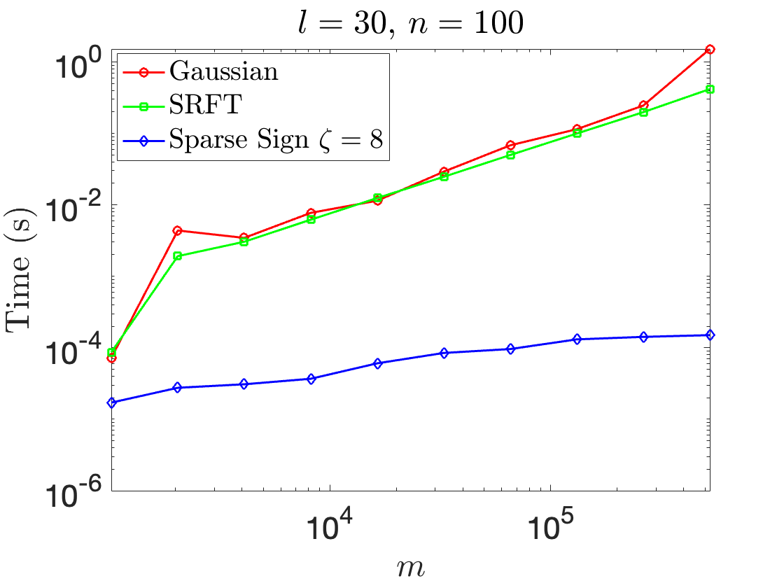
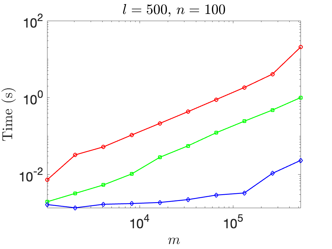
2.5.1 Computational speeds of different embeddings
Here, we compare the empirical efficiency of constructing sketches with some common randomized embeddings listed in Table 2.1. We consider applying an embedding of size to a matrix of size , which can be interpreted as embedding vectors in an ambient space to a lower dimensional space . We scale the experiments with respect to the ambient dimension , at several different embedding dimensions , with a fixed number of repetitions . Figure 2.1 suggests that, with proper implementation, the sparse sign matrices are more efficient than the Gaussian embeddings and the SRTTs, especially for large-scale problems. The SRTTs outperform Gaussian embeddings in terms of efficiency, and such an advantage can be amplified as increases. These observations align with the asymptotic complexity in Table 2.1. While we also observe that, with MATLAB default implementation, the Gaussian embeddings usually enjoy matching efficiency as sparse sign matrices for moderate-size problems, and are more efficient than SRTTs.

2.5.2 Computational speeds of different pivoting schemes
Given a sketch of , we isolate different pivoting schemes in Algorithm 1 and compare their run time as the problem size increases. Specifically, the LUPP and CPQR pivot directly on the given row sketch , while the DEIM involves one additional power iteration with orthogonalization (Section 2.2.4) before applying the LUPP (i.e., with a given column sketch , for DEIM, we first construct an orthonormal basis for columns of the sketch, and then we compute the reduced SVD for , and finally we column-wisely pivot on the resulting right singular vectors of size ).
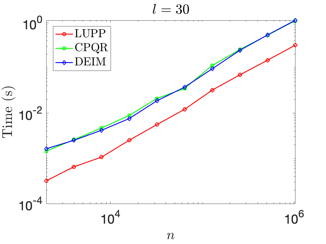
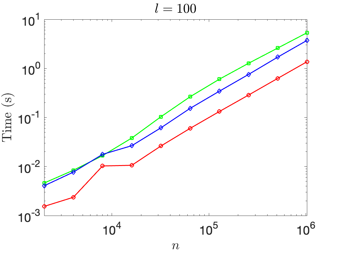
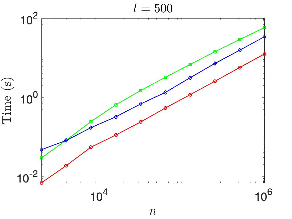
In Figure 2.2, we observe a considerable run time advantage of the LUPP over the CPQR and DEIM, especially when is large. (Additionally, we see that DEIM slightly outperforms CPQR, which is perhaps surprising, given the substantially larger number of flops required by DEIM.)
2.5.3 Randomized skeleton selection algorithms: accuracy and efficiency
As we move from measuring speed to measuring the precision of revealing the numerical rank of a matrix, the choice of test matrix becomes important. We consider four different classes of test matrices, including some synthetic random matrices with different spectral patterns, as well as some empirical datasets, as summarized below:
-
1.
large: a full-rank sparse matrix with nonzero entries from the SuiteSparse matrix collection, generated by a linear programming problem sequence [104].
-
2.
YaleFace64x64: a full-rank dense matrix, consisting of face images each of size . The flattened image vectors are centered and normalized such that the average image vector is zero, and the entries are bounded within .
-
3.
MNIST training set consists of images of hand-written digits from to . Each image is of size . The images are flattened and normalized to form a full-rank matrix of size where is the number of images and is the size of the flattened images, with entries bounded in . The nonzero entries take approximately of the matrix for both the training and the testing sets.
-
4.
Random sparse non-negative (SNN) matrices are synthetic random sparse matrices used in [153, 137] for testing skeleton selection algorithms. Given , a random SNN matrix of size takes the form,
(2.20) where , , are random sparse vectors with non-negative entries. In the experiments, we use two random SNN matrices of distinct sizes:
-
(i)
SNN1e3 is a SNN matrix with , for , and for ;
-
(ii)
SNN1e6 is a SNN matrix with , for , and for .
-
(i)
Scaled with respect to the approximation ranks , we compare the accuracy and efficiency of the following randomized CUR algorithms:
-
1.
Rand-LUPP (and Rand-LUPP-1piter): Algorithm 1 with being a row sketch (or with one plain power iteration as in Equation 2.14), and pivoting with LUPP;
-
2.
Rand-CPQR (and Rand-CPQR-1piter): Algorithm 1 with being a row sketch (or with one power iteration as in Equation 2.14), and pivoting with CPQR [153];
-
3.
RSVD-DEIM: Algorithm 1 with being an approximation of leading- right singular vectors (Equation 2.16), and pivoting with LUPP [137];
-
4.
RSVD-LS: Skeleton sampling based on approximated leverage scores [96] from a rank- SVD approximation (Equation 2.16);
-
5.
SRCUR: Spectrum-revealing CUR decomposition proposed in [25].
The asymptotic complexities of the first three randomized pivoting-based skeleton selection algorithms based on Algorithm 1 are summarized in Table 2.2.
| Algorithm | Row basis approximator construction (Line 1,2) | Pivoting (Line 3) |
|---|---|---|
| Rand-LUPP | ||
| Rand-LUPP-1piter | ||
| Rand-CPQR | ||
| Rand-CPQR-1piter | ||
| RSVD-DEIM |
For consistency, we use Gaussian embeddings for sketching throughout the experiments. With the selected column and row skeletons, we leverage the stable construction in Equation 2.10 to form the corresponding CUR decompositions . Although oversampling (i.e., ) is necessary for multiplicative error bounds with respect to the optimal rank- approximation error (Equation 2.13, Theorem 2.1), since oversampling can be interpreted as a shift of curves along the axis of the approximation rank, for the comparison purpose, we simply treat , and compare the rank- approximation errors of the CUR decompositions against the optimal rank- approximation error .
From Figure 2.3-2.6, we observe that the randomized pivoting-based skeleton selection algorithms that fall in Algorithm 1 (i.e., Rand-LUPP, Rand-CPQR, and RSVD-DEIM) share the similar approximation accuracy, which is considerably higher than that of the RSVD-LS and SRCUR. From the efficiency perspective, Rand-LUPP provides the most competitive run time among all the algorithms, especially when is sparse. Meanwhile, we observe that, for both Rand-CPQR and Rand-LUPP, constructing the sketches with one plain power iteration (i.e., with Equation 2.14) can observably improve the accuracy, without sacrificing the efficiency significantly (e.g., in comparison to the randomized DEIM which involves one power iteration with orthogonalization as in Section 2.2.4).
In Figure 2.7, a similar performance is also observed on a synthetic large-scale problem, SNN1e6, where the matrix is only accessible as a fast matrix-vector multiplication (matvec) oracle such that each matvec takes (i.e., in our construction) operations. It is worth noticing that the gap between the optimal rank- approximation error and the CUR approximation error consists of two components: (i) the suboptimality of skeleton selection from the algorithms, and (ii) the gap between the optimal rank- approximation error and the CUR approximation error with the optimal skeleton selection from the matrix skeletonization problem. Despite the unknown optimal skeleton selection due to its intractability [29], intuitively, the suboptimality from the matrix skeletonization problem itself accounts for the larger CUR approximation error in Figure 2.7 (cf. Figure 2.3-2.6) due to the significantly more challenging skeleton selection problem brought by the large matrix size .
Chapter 3 Randomized Subspace Approximations: Efficient Bounds and Estimates for Canonical Angles
Abstract
Randomized subspace approximation with “matrix sketching” is an effective approach for constructing approximate partial singular value decompositions (SVDs) of large matrices.
The performance of such techniques has been extensively analyzed, and very precise estimates on the distribution of the residual errors have been derived.
However, our understanding of the accuracy of the computed singular vectors (measured in terms of the canonical angles between the spaces spanned by the exact and the computed singular vectors, respectively) remains relatively limited.
In this work, we present bounds and estimates for canonical angles of randomized subspace approximation that can be computed efficiently either a priori or a posteriori.
Under moderate oversampling in the randomized SVD, our prior probabilistic bounds are asymptotically tight and can be computed efficiently, while bringing a clear insight into the balance between oversampling and power iterations given a fixed budget on the number of matrix-vector multiplications.
The numerical experiments demonstrate the empirical effectiveness of these canonical angle bounds and estimates on different matrices under various algorithmic choices for the randomized SVD.111This chapter is based on the following arXiv paper:
\bibentrydong2022efficient [46].
3.1 Introduction
In light of the ubiquity of high-dimensional data in modern computation, dimension reduction tools like the low-rank matrix decompositions are becoming indispensable tools for managing large data sets. In general, the goal of low-rank matrix decomposition is to identify bases of proper low-dimensional subspaces that well encapsulate the dominant components in the original column and row spaces. As one of the most well-established forms of matrix decompositions, the truncated singular value decomposition (SVD) is known to achieve the optimal low-rank approximation errors for any given ranks [55]. Moreover, the corresponding left and right leading singular subspaces can be broadly leveraged for problems like principal component analysis, canonical correlation analysis, spectral clustering [20], and leverage score sampling for matrix skeleton selection [50, 96, 49].
However, for large matrices, the computational cost of classical algorithms for computing the SVD (cf. [144, Lec. 31] or [59, Sec. 8.6.3]) quickly becomes prohibitive. Fortunately, a randomization framework known as “matrix sketching” [68, 165] provides a simple yet effective remedy for this challenge by embedding large matrices to random low-dimensional subspaces where the classical SVD algorithms can be executed efficiently.
Concretely, for an input matrix and a target rank , the basic version of the randomized SVD [68, Alg. 4.1] starts by drawing a Gaussian random matrix for a sample size that is slightly larger than so that . Then through a matrix-matrix multiplication with complexity, the -dimensional row space of is embedded to a random -dimensional subspace. With the low-dimensional range approximation , a rank- randomized SVD can be constructed efficiently by computing the QR and SVD of small matrices in time. When the spectral decay in is slow, a few power iterations (usually ) can be incorporated to enhance the accuracy, cf. [68] Algorithms 4.3 and 4.4.
Let 222 Here , , and . is a diagonal matrix with positive non-increasing diagonal entries, and . denote the (unknown) full SVD of . In this work, we explore the alignment between the true leading rank- singular subspaces and their respective rank- approximations in terms of the canonical angles and . We introduce prior statistical guarantees and unbiased estimates for these angles with respect to , as well as posterior deterministic bounds with the additional dependence on , as synopsized below.
3.1.1 Our Contributions
Prior probabilistic bounds and estimates with insight on oversampling-power iteration balance.
Evaluating the randomized SVD with a fixed budget on the number of matrix-vector multiplications, the computational resource can be leveraged in two ways – oversampling (characterized by ) and power iterations (characterized by ). A natural question is how to distribute the computation between oversampling and power iterations for better subspace approximations?
Answers to this question are problem-dependent: when aiming to minimize the canonical angles between the true and approximated leading singular subspaces, the prior probabilistic bounds and estimates on the canonical angles provide primary insights. To be precise, with isotropic random subspace embeddings and sufficient oversampling, the accuracy of subspace approximations depends jointly on the spectra of the target matrices, oversampling, and the number of power iterations. In this work, we present a set of prior probabilistic bounds that precisely quantify the relative benefits of oversampling versus power iterations. Specifically, the canonical angle bounds in Theorem 3.1
-
(i)
provide statistical guarantees that are asymptotically tight under sufficient oversampling (i.e., ),
-
(ii)
unveil a clear balance between oversampling and power iterations for random subspace approximations with given spectra,
-
(iii)
can be evaluated in time given access to the (true/estimated) spectra and provide valuable estimations for canonical angles in practice with moderate oversampling (e.g., ).
Further, inspired by the derivation of the prior probabilistic bounds, we propose unbiased estimates for the canonical angles with respect to given spectra that admit efficient evaluation and concentrate well empirically.
Posterior residual-based guarantees.
Alongside the prior probabilistic bounds, we present two sets of posterior canonical angle bounds that hold in the deterministic sense and can be approximated efficiently based on the residuals and the spectrum of .
Numerical comparisons.
With numerical comparisons among different canonical angle bounds on a variety of data matrices, we aim to explore the question on how the spectral decay and different algorithmic choices of randomized SVD affect the empirical effectiveness of different canonical angle bounds. In particular, our numerical experiments suggest that, for matrices with subexponential spectral decay, the prior probabilistic bounds usually provide tighter (statistical) guarantees than the (deterministic) guarantees from the posterior residual-based bounds, especially with power iterations. By contrast, for matrices with exponential spectral decay, the posterior residual-based bounds can be as tight as the prior probabilistic bounds, especially with large oversampling. The code for numerical comparisons is available at https://github.com/dyjdongyijun/Randomized_Subspace_Approximation.
3.1.2 Related Work
The randomized SVD algorithm (with power iterations) [99, 68] has been extensively analyzed as a low-rank approximation problem where the accuracy is usually measured in terms of residual norms, as well as the discrepancy between the approximated and true spectra [68, 64, 98, 101]. For instance, [68, Thm. 10.7, Thm. 10.8] show that for a given target rank (usually for the randomized acceleration to be useful), a small constant oversampling is sufficient to guarantee that the residual norm of the resulting rank- approximation is close to the optimal rank- approximation (i.e., the rank- truncated SVD) error with high probability. Alternatively, [64] investigates the accuracy of the individual approximated singular values and provides upper and lower bounds for each with respect to the true singular value .
In addition to providing accurate low-rank approximations, the randomized SVD algorithm also produces estimates of the leading left and right singular subspaces corresponding to the top singular values. When coupled with power iterations ([68] Algorithms 4.3 & 4.4), such randomized subspace approximations are commonly known as randomized power (subspace) iterations. Their accuracy is explored in terms of canonical angles that measure differences between the unknown true subspaces and their random approximations [20, 123, 109]. Generally, upper bounds on the canonical angles can be categorized into two types: (i) probabilistic bounds that establish prior statistical guarantees by exploring the concentration of the alignment between random subspace embeddings and the unknown true subspace, and (ii) residual-based bounds that can be computed a posteriori from the residual of the resulting approximation.
The existing prior probabilistic bounds on canonical angles [20, 123] mainly focus on the setting where the randomized SVD is evaluated without oversampling or with a small constant oversampling. Concretely, [20] derives guarantees for the canonical angles evaluated without oversampling (i.e., ) in the context of spectral clustering. Further, by taking a small constant oversampling (e.g., ) into account, Saibaba [123] provides a comprehensive analysis for an assortment of canonical angles between the true and approximated leading singular spaces. Compared with our results (Theorem 3.1), in both no-oversampling and constant-oversampling regimes, the basic forms of the existing prior probabilistic bounds (e.g., [123] Theorem 1) generally depend on the unknown singular subspace . Although such dependence is later lifted using the isotropicity and the concentration of the randomized subspace embedding (e.g., [123] Theorem 6), the separated consideration on the spectra and the singular subspaces introduces unnecessary compromise to the upper bounds (as we will discuss in Remark 3.1). In contrast, by allowing a more generous choice of multiplicative oversampling , we present a set of space-agnostic bounds (i.e., bounds that hold regardless of the singular vectors of ) based on an integrated analysis of the spectra and the singular subspaces that appears to be tighter both from derivation and in practice.
The classical Davis-Kahan and theorems [38] for eigenvector perturbation can be used to compute deterministic and computable bounds for the canonical angles. These bounds have the advantage that they give strict bounds (up to the estimation of the so-called gap) rather than estimates or bounds that hold with high probability (although, as we argue below, the failure probability can be taken to be negligibly low). The Davis-Kahan theorems have been extended to perturbation of singular vectors by Wedin [161], and recent work [109] derives perturbation bounds for singular vectors computed using a subspace projection method. In this work, we establish canonical angle bounds for the singular vectors in the context of (randomized) subspace iterations. Our results indicate clearly that the accuracy of the right and left singular vectors are usually not identical (i.e., is more accurate with Algorithm 4).
As a roadmap, we formalize the problem setup in Section 3.2, including a brief review of the randomized SVD and canonical angles. In Section 3.3, we present the prior probabilistic space-agnostic bounds. Subsequently, in Section 3.4, we describe a set of unbiased canonical angle estimates that is closely related to the space-agnostic bounds. Then in Section 3.5, we introduce two sets of posterior residual-based bounds. Finally, in Section 3.6, we instantiate the insight cast by the space-agnostic bounds on the balance between oversampling and power iterations and demonstrate the empirical effectiveness of different canonical angle bounds and estimates with numerical comparisons.
3.2 Problem Setup
In this section, we first recapitulate the randomized SVD algorithm (with power iterations) [68] for which we analyze the accuracy of the resulting singular subspace approximations. Then, we review the notion of canonical angles [59] that quantify the difference between two subspaces of the same Euclidean space.
3.2.1 Notation
We start by introducing notations for the SVD of a given matrix of rank :
For any , we let and denote the orthonormal bases of the dimension- left and right singular subspaces of corresponding to the top- singular values, while and are orthonormal bases of the respective orthogonal complements. The diagonal submatrices consisting of the spectrum, and , follow analogously.
Meanwhile, for the QR decomposition of an arbitrary matrix (), we denote such that and consist of orthonormal bases of the subspace spanned by the columns of and its orthogonal complement.
Furthermore, we denote the spectrum of by , a diagonal matrix with singular values on the diagonal.
Generally, we adapt the MATLAB notation for matrix slicing throughout this work. For any , we denote .
3.2.2 Randomized SVD and Power Iterations
As described in Algorithm 4, the randomized SVD provides a rank- () approximation of while grants provable acceleration to the truncated SVD evaluation – with the Gaussian random matrix333Asymptotically, there exist deterministic iterative algorithms for the truncated SVD (e.g., based on Lanczos iterations ([144] Algorithm 36.1)) that run in time. However, compared with these inherently sequential iterative algorithms, the randomized SVD can be executed much more efficiently in practice, even with power iterations (i.e., ), since the computation bottleneck in Algorithm 4 involves only matrix-matrix multiplications which are easily parallelizable and highly optimized.. Such efficiency improvement is achieved by first embedding the high-dimensional row (column) space of to a low-dimensional subspace via a Johnson-Lindenstrauss transform444Throughout this work, we focus on Gaussian random matrices (Algorithm 4, Line 1) in the sake of theoretical guarantees, i.e., being isotropic and rotationally invariant. (JLT) (known as “sketching”). Then, SVD of the resulting column (row) sketch can be evaluated efficiently in time, and the rank- approximation can be constructed accordingly.
The spectral decay in has a significant impact on the accuracy of the resulting low-rank approximation from Algorithm 4 (as suggested in [68] Theorem 10.7 and Theorem 10.8). To remediate the performance of Algorithm 4 on matrices with flat spectra, power iterations (Algorithm 4, Line 2) are usually incorporated to enhance the spectral decay. However, without proper orthogonalization, plain power iterations can be numerically unstable, especially for ill-conditioned matrices. For stable power iterations, starting with of full column rank (which holds almost surely for Gaussian random matrices), we incorporate orthogonalization in each power iteration via the reduced unpivoted QR factorization (each with complexity ). Let be an orthonormal basis of produced by the QR factorization. Then, the stable evaluation of power iterations (Algorithm 4, Line 2) can be expressed as:
| (3.1) |
Notice that in Algorithm 4, with , the approximated rank- SVD of can be expressed as where . With and characterizing the approximated -dimensional left and right leading singular subspaces, and denote an arbitrary pair of their respective orthogonal complements. For any , we further denote the partitions and where and , respectively.
3.2.3 Canonical Angles
Now, we review the notion of canonical angles [59] that measure distances between two subspaces , of an arbitrary Euclidean space .
Definition 3.1 (Canonical angles, [59]).
Given two subspaces with dimensions and (assuming without loss of generality), the canonical angles, denoted by , consist of angles that measure the alignment between and , defined recursively such that
| s.t. | |||
For arbitrary full-rank matrices and (assuming without loss of generality), let denote the canonical angles between the corresponding spanning subspaces in . For each , let be the -th (smallest) canonical angle such that and (cf. [183] Section 3).
With the unknown true rank- truncated SVD and an approximated rank- SVD from Algorithm 4, in this work, we mainly focus on the prior and posterior guarantees for the canonical angles and . Meanwhile, in Theorem 3.4, we present a set of posterior residual-based upper bounds for the canonical angles and as corollaries.
3.3 Space-agnostic Bounds under Sufficient Oversampling
We start by pointing out the intuition that, under sufficient oversampling, with Gaussian random matrices whose distribution is orthogonally invariant, the alignment between the approximated and true subspaces are independent of the unknown true subspaces, i.e., the canonical angles are space-agnostic, as reflected in the following theorem.
Theorem 3.1.
For a rank- randomized SVD (Algorithm 4) with a Gaussian embedding and power iterations, when the oversampled rank satisfies (where is the target rank, ) and is reasonably small such that 555Notice that . To the extremes, when the tail is flat ; while when for all . In particular, with a relatively flat tail and a reasonably small (recall that is usually sufficient in practice), we have , and the assumption can be simplified as . Although exponential tail decay can lead to small and may render the assumption infeasible in theory, in practice, simply taking , , and is sufficient to ensure the validity of upper bounds when even for matrices with rapid tail decay, as shown in Section 3.6.2. satisfies , with high probability (at least ), there exist distortion factors such that
| (3.2) | ||||
| (3.3) |
for all , where and . Furthermore, both bounds are asymptotically tight:
| (3.4) | ||||
| (3.5) |
where suppresses the distortion factors 666 Despite the asymptotic tightness of Theorem 3.1 theoretically, in practice, we observe that the empirical validity of lower bounds is more restrictive on oversampling than that of upper bounds. In specific, the numerical observations in Section 3.6.2 suggest that is usually sufficient for the upper bounds to hold; whereas the empirical validity of lower bounds generally requires more aggressive oversampling of at least , also with slightly larger constants associated with and , as demonstrated in Section A.2.1. .
The main insights provided by Theorem 3.1 include: (i) improved statistical guarantees for canonical angles under sufficient oversampling (i.e., ), as discussed later in Remark 3.1, (ii) a clear view of the balance between oversampling and power iterations for random subspace approximations with given spectra, as instantiated in Section 3.6.3, and (iii) affordable upper bounds that can be evaluated in time with access to the (true/estimated) spectra and hold in practice with only moderate oversampling (e.g., ), as shown in Section 3.6.2.
Proof of Theorem 3.1.
We show the derivation of Equation 3.2 for left canonical angles . The derivation for right canonical angles in Equation 3.3 follows directly by replacing the exponent in Equation 3.2 with in Equation 3.3. This slightly larger exponent comes from the additional half power iteration associated with in Algorithm 4 (as discussed in Remark 3.3), an observation made also in [123].
For the rank- randomized SVD with a Gaussian embedding and power iterations, we denote the projected embeddings onto the singular subspaces and , as well as their weighted correspondences and , such that
Then for all ,
Since is assumed to have full column rank, we have (which is an orthogonal projection), and
Therefore for all ,
| (3.6) | ||||
By the orthogonal invariance of the distribution of Gaussian embeddings together with the orthonormality of , we see that and are independent Gaussian random matrices with the same entry-wise i.i.d. distribution as . Therefore by Lemma A.1, when , with high probability (at least ),
for some .
Analogously, when , with high probability (at least ),
for some .
Therefore by the union bound, we have with high probability (at least ) that,
which leads to Equation 3.2, while the tightness is implied by
The proof of Equation 3.3 follows analogously by replacing the exponents and with and , respectively. ∎
Remark 3.1 (Comparison with existing probabilistic bounds).
With access to the unknown right singular subspace , let and . Then, Saibaba [123, Thm. 1]indicates that, for all ,
| (3.7) | ||||
| (3.8) |
Further, leveraging existing results on concentration properties of the independent and isotropic Gaussian random matrices and (e.g., from the proof of [68] Theorem 10.8), [123] shows that, when , for any , with probability at least ,
Without loss of generality, we consider the bounds on . Comparing to the existing bound in Equation 3.7, under multiplicative oversampling (, ), Equation 3.2 in Theorem 3.1 captures the spectral decay on the tail by replacing the denominator term
We observe that ; while Lemma A.1 implies that, for independent Gaussian random matrices and with i.i.d. entries from ,
With non-negligible spectral decay on the tail such that , when , Equation 3.2 provides a tighter statistical guarantee than Equation 3.7, which is also confirmed by numerical observations in Section 3.6.2.
From the derivation perspective, such improvement is achieved by taking an integrated view on the concentration of , instead of considering the spectrum and the unknown singular subspace separately.
3.4 Unbiased Space-agnostic Estimates
A natural corollary from the proof of Theorem 3.4 is unbiased estimates for the canonical angles that hold for arbitrary oversampling (i.e., for all ). Further, we will subsequently see in Section 3.6 that such unbiased estimates also enjoy good empirical concentration.
Proposition 3.2.
For a rank- randomized SVD (Algorithm 4) with the Gaussian embedding such that and power iterations, for all ,
| (3.9) |
and analogously,
| (3.10) |
where and are independent Gaussian random matrices with i.i.d. entries drawn from .
To calculate the unbiased estimate, for a modest integer we draw a set of independent Gaussian random matrices and evaluate
for all , which can be conducted efficiently in time. Algorithm 5 demonstrates the construction of unbiased estimates for ; while the unbiased estimates for can be evaluated analogously by replacing Line 4 with , .
As demonstrated in Section 3.6, the unbiased estimates concentrate well in practice such that a sample size as small as is seen to be sufficient to provide good estimates. Further, with independent Gaussian random matrices, the unbiased estimates in Proposition 3.2 are also space agnostic, i.e., Equation 3.9 and Equation 3.10 only depend on the spectrum but not on the unknown true singular subspaces and .
Proof of Proposition 3.2.
To show Equation 3.9, we recall from the proof of Theorem 3.1 that, for the rank- randomized SVD with a Gaussian embedding and power iterations, and are independent Gaussian random matrices with the same entry-wise distribution as . Therefore, with , for all ,
The unbiased estimate in Equation 3.10 follows analogously. ∎
As a side note, we point out that, compared with the probabilistic upper bounds Equation 3.2 and Equation 3.3, the estimates Equation 3.9 and Equation 3.10 circumvent overestimation from the operator-convexity of inversion ,
which implies that
3.5 Posterior Residual-based Bounds
In addition to the prior probabilistic bounds and unbiased estimates, in this section, we introduce two sets of posterior guarantees for the canonical angles that hold deterministically and can be evaluated/approximated efficiently based on the residual of the resulting low-rank approximation from Algorithm 4.
Remark 3.2 (Generality of residual-based bounds).
It is worth highlighting that both the statements and the proofs of the posterior guarantees Theorems 3.3 and 3.4 to be presented are algorithm-independent. In contrast to Theorem 3.1 and Proposition 3.2 whose derivation depends explicitly on the algorithm (e.g., assuming being Gaussian in Algorithm 4), the residual-based bounds in Theorems 3.3 and 3.4 hold for general low-rank approximations .
We start with the following proposition that establishes relations between the canonical angles and the residuals and the true spectrum .
Theorem 3.3.
Given any and with orthonormal columns such that and , we have for each (),
| (3.11) |
while
| (3.12) |
Remark 3.3 (Left versus right singular subspaces).
When and consist of approximated left and right singular vectors from Algorithm 4, upper bounds on tend to be smaller than those on . This is induced by the algorithmic fact that, in Algorithm 4, is an orthonormal basis of , while and are orthonormal bases of . That is, the evaluation of is enhanced by an additional half power iteration compared with that of , which is also reflected by the differences in exponents on (i.e., versus ) in Theorem 3.1 and Proposition 3.2. This difference can be important especially when is small (e.g., ). When higher accuracy in the left singular subspace is desirable, one can work with .
Proof of Theorem 3.3.
Starting with the leading left singular subspace, by definition, for each , we have
Then, we observe that the following holds simultaneously,
where and . Finally by Lemma A.2, we have
Meanwhile, the upper bound for the leading right singular subspace can be derived analogously by observing that
∎
As a potential drawback, although the residuals and in Theorem 3.3 can be evaluated efficiently in and time777 For the complexity of computing , we assume that is readily available from Algorithm 4. Otherwise (e.g., when Algorithm 4 returns but not ), the evaluation of will inevitably take as that of . , respectively, the exact evaluation of their full spectra can be unaffordable. A straightforward remedy for this problem is to use only the second terms in the right-hand-sides of Equation 3.11 and Equation 3.12 while estimating and with the randomized power method (cf. [86], [101] Algorithm 4). Alternatively, we leverage the analysis from [109] Theorem 6.1 and present the following posterior bounds based only on norms of the residuals which can be estimated efficiently via sampling.
Theorem 3.4.
For any rank- approximation in the SVD form (not necessarily obtained by Algorithm 4), recall the notation that , , while are the orthogonal complements of , respectively. Then, with , , and , assuming and , we define the spectral gaps
Then for an arbitrary unitarily invariant norm ,
| (3.13) | ||||
| (3.14) |
and specifically for the spectral or Frobenius norm (),
| (3.15) | ||||
| (3.16) |
Furthermore, for all ,
| (3.17) | ||||
| (3.18) | ||||
| (3.19) | ||||
| (3.20) |
In practice, norms of the residuals can be computed as
where the construction of , , and takes time, while the respective norms can be estimated efficiently via sampling (cf. [101] Algorithm 1-4, [105] Algorithm 1-3, etc.).
The proof of Theorem 3.4 is similar to that of [109, Thm. 6.1].
Proof of Theorem 3.4.
Let , , , and , , and . We start by expressing the canonical angles in terms of and :
By observing that for any rank- approximation in the SVD form ,
we left multiply and right multiply on both sides and get
| (3.21) |
while left multiplying and right multiplying yield
| (3.22) |
Bounding and .
To bound , we observe the following from the third row of Equation 3.21 and the third column of Equation 3.22,
Noticing that and , we have
for all , which implies that
and leads to
where the second line follows from Lemma A.3. These lead to Equations 3.13 and 3.17
Bounding and .
To bound , we leverage the second row of Equation 3.21 and the second column of Equation 3.22,
Up to rearrangement, we observe that
which implies that
and therefore, with Lemma A.3, for all ,
Then, with the stronger inequality for the spectral or Frobenius norm (),
leads to Equation 3.15. Meanwhile for Equation 3.19, the individual canonical angles are upper bounded by
Analogously, by observing that
we have that, by Lemma A.3, for all ,
and therefore for the spectral or Frobenius norm (),
which leads to Equation 3.16. Additionally for individual canonical angles ,
This yields Equation 3.20 and completes the proof. ∎
3.6 Numerical Experiments
First, we present numerical comparisons among different canonical angle upper bounds and the unbiased estimates on the left and right leading singular subspaces of various synthetic and real data matrices. We start by describing the target matrices in Section 3.6.1. In Section 3.6.2, we discuss the performance of the unbiased estimates, as well as the relative tightness of the canonical angle bounds, for different algorithmic choices based on the numerical observations. Second, in Section 3.6.3, we present an illustrative example that provides insight into the balance between oversampling and power iterations brought by the space-agnostic bounds.
3.6.1 Target Matrices
We consider several different classes of target matrices, including some synthetic random matrices with different spectral patterns, as well as an empirical dataset, as summarized below:
-
1.
A random sparse non-negative (SNN) matrix [138] of size takes the form,
(3.23) where and control the spectral decay, and , are random sparse vectors with non-negative entries. In the experiments, we test on two random SNN matrices of size with and , respectively.
-
2.
Gaussian dense matrices with controlled spectral decay are randomly generated via a similar construction to the SNN matrix, with and in (3.23) replaced by uniformly random dense orthonormal vectors. The generating procedures for with rank can be summarized as following:
-
(i)
Draw Gaussian random matrices, and .
-
(ii)
Compute , as orthonormal bases.
-
(iii)
Given the spectrum , we construct .
In the experiments, we consider two types of spectral decay:
-
(i)
slower decay with , for all , for all , and
-
(ii)
faster decay with , for all , for all .
-
(i)
-
3.
MNIST training set consists of images of hand-written digits from to . Each image is of size . We form the target matrices by uniformly sampling images from the MNIST training set. The images are flattened and normalized to form a full-rank matrix of size where is the size of the flattened images, with entries bounded in . The nonzero entries take approximately of the matrix for both the training and the testing sets.
3.6.2 Canonical Angle Bounds and Estimates
Now we present numerical comparisons of the performance of the canonical angle bounds and the unbiased estimates under different algorithmic choices. Considering the scenario where the true matrix spectra may not be available in practice, we calculate two sets of upper bounds, one from the true spectra and the other from the approximated singular values from Algorithm 4. For the later, we pad the approximated spectrum with copies of and evaluate the canonical angle bounds and estimates with .
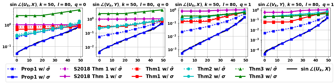
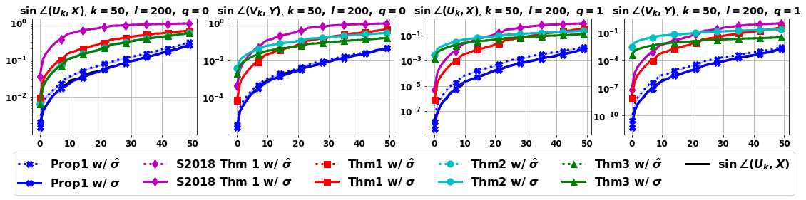
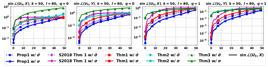
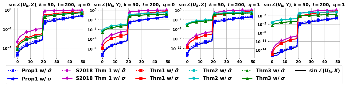
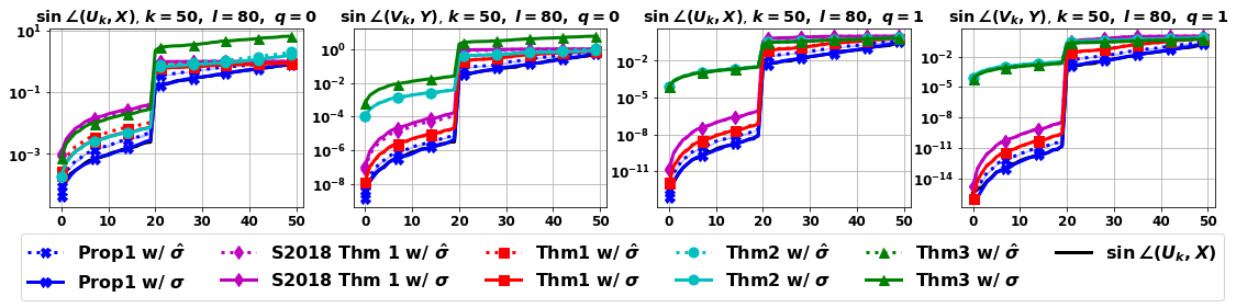
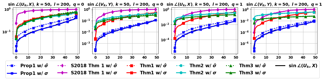
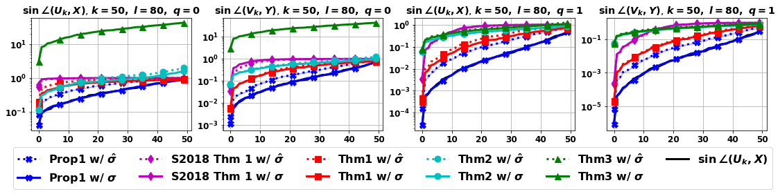
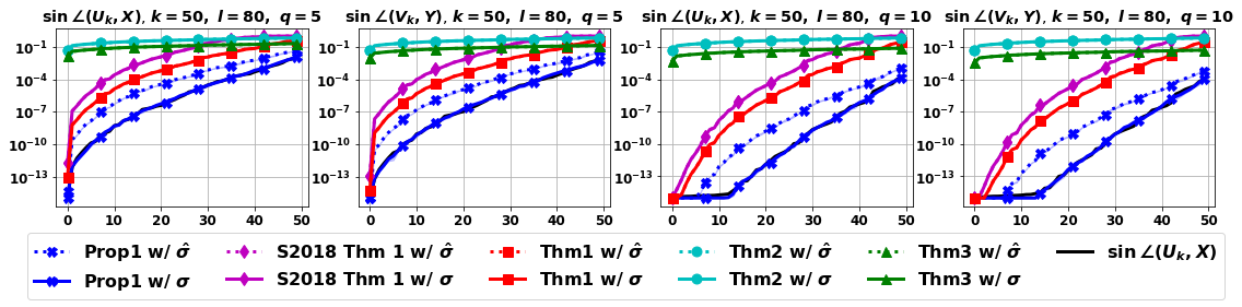
From Figure 3.1 to Figure 3.11,
-
1.
Red lines and dashes (Thm1 w/ and ) represent the space-agnostic probabilistic bounds in Theorem 3.1 evaluated with the true (lines) and approximated (dashes) singular values, , and , respectively, where we simply ignore tail decay and suppress constants for the distortion factors and set and in Equations 3.2 and 3.3;
-
2.
Blue lines and dashes (Prop1 w/ and ) represent the unbiased space-agnostic estimates in Proposition 3.2 (averages of independent trials with blue shades marking the corresponding minima and maxima in the trials) evaluated with the true (lines) and approximated (dashes) singular values, and , respectively;
-
3.
Cyan lines and dashes (Thm2 w/ and ) represent the posterior residual-based bounds in Theorem 3.3 evaluated with the true (lines) and approximated (dashes) singular values, , and , respectively;
-
4.
Green lines and dashes (Thm3 w/ and ) represent the posterior residual-based bounds Equation 3.13 and Equation 3.14 in Theorem 3.4 evaluated with the true (lines) and approximated (dashes) singular values, , and , respectively;
-
5.
Magenta lines and dashes (S2018 Thm1 w/ and ) represent the upper bounds in [123] Theorem 1 (i.e., Equation 3.7 and Equation 3.8) evaluated with the true (lines) and approximated (dashes) singular values, and , respectively, and the unknown true singular subspace such that and ;
-
6.
Black lines mark the true canonical angles .
We recall from Remark 3.3 that, by the algorithmic construction of Algorithm 4, for given , canonical angles of the right singular spaces are evaluated with half more power iterations than those of the left singular spaces . That is, , with in Figure 3.1-Figure 3.10 can be viewed as canonical angles of randomized subspace approximation with power iterations, respectively; while Figure 3.11 corresponds to randomized subspace approximations constructed with power iterations analogously.
For each set of upper bounds/unbiased estimates, we observe the following.
-
1.
The space-agnostic probabilistic bounds (Thm1 w/ and ) in Theorem 3.1 provide tighter statistical guarantees for the canonical angles of all the tested target matrices in comparison to those from [123] Theorem 1 (S2018 Thm1 w/ and ) , as explained in Remark 3.1.
-
2.
The unbiased estimators (Prop1 w/ and ) in Proposition 3.2 yield accurate approximations for the true canonical angles on all the tested target matrices with as few as trials, while enjoying good empirical concentrate. As a potential drawback, the accuracy of the unbiased estimates may be compromised when approaching the machine epsilon (as observed in Figure 3.7, ).
-
3.
The posterior residual-based bounds (Thm2 w/ and ) in Theorem 3.3 are relatively tighter among the compared bounds in the setting with larger oversampling (), and no power iterations ( with ) or exponential spectral decay (Figure 3.3)
-
4.
The posterior residual-based bounds Equations 3.13 and 3.14 (Thm3 w/ and ) in Theorem 3.4 share the similar relative tightness as the posterior residual-based bounds in Theorem 3.3, but are slightly more sensitive to power iterations. As shown in Figure 3.3, on a target matrix with exponential spectral decay and large oversampling (), Theorem 3.4 gives tighter posterior guarantees when . However, with the addition assumptions and , Theorem 3.4 usually requires large oversampling () in order to provide non-trivial (i.e., within the range ) bounds.
For target matrices with various patterns of spectral decay, with different combinations of oversampling () and power iterations (), we make the following observations on the relative tightness of upper bounds in Theorem 3.1, Theorem 3.3, and Theorem 3.4.
-
1.
For target matrices with subexponential spectral decay, the space-agnostic bounds in Theorem 3.1 are relatively tighter in most tested settings, except for the setting in Figure 3.3 with larger oversampling () and no power iterations ().
-
2.
For target matrices with exponential spectral decay (Figure 3.3 and Figure 3.4), the posterior residual-based bounds in Theorem 3.3 and Theorem 3.4 tend to be relatively tighter, especially with large oversampling (Figure 3.3 with ). Meanwhile, with power iterations , Theorem 3.4 tend to be tighter than Theorem 3.3.
Furthermore, considering the scenario with an unknown true spectrum , we plot estimations for the upper bounds in Theorem 3.1, Theorem 3.3, Theorem 3.4, and the unbiased estimates in Proposition 3.2, evaluated with a padded approximation of the spectrum , which leads to mild overestimations, as marked in dashes from Figure 3.1 to Figure 3.11.
3.6.3 Balance between Oversampling and Power Iterations
To illustrate the insight cast by Theorem 3.1 on the balance between oversampling and power iterations, we consider the following synthetic example.
Example 1.
Given a target rank , we consider a simple synthetic matrix of size , consisting of random singular subspaces (generated by orthonormalizing Gaussian matrices) and a step spectrum:
We fix a budget of matrix-vector multiplications with in total. The goal is to distribute the computational budget between the sample size and the number of power iterations for the smaller canonical angles .
Leveraging Theorem 3.1, we start by fixing associated with the constants and in Equation 3.2 such that and . Characterized by , the right-hand-side of Equation 3.2 under fixed budget (i.e., ) is defined as:
| (3.24) | ||||
With the synthetic step spectrum, the dependence of Equation 3.2 on is reduced to the spectral gap in Equation 3.24.
As a synopsis, Table 3.1 summarizes the relevant parameters that characterize the problem setup.
| budget parameter | ||
| size parameter | ||
| oversampling parameter | and |
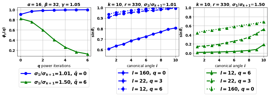
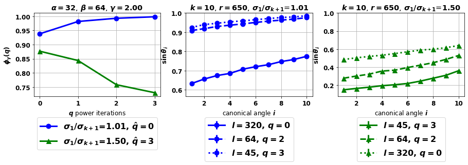
With , , , and , Figure 3.12 and Figure 3.13 illustrate (i) how the balance between oversampling and power iterations is affected by the spectral gap , and more importantly, (ii) how Equation 3.24 unveils the trend in true canonical angles among different configurations .
Concretely, both Figure 3.12 and Figure 3.13 imply that more oversampling (e.g., ) is preferred when the spectral gap is small (e.g., ); while more power iterations (e.g., ) are preferred when the spectral gap is large (e.g., ). Such trends are both observed in the true canonical angles () and well reflected by .
3.7 Discussion
We presented prior and posterior bounds and estimates that can be computed efficiently for canonical angles of the randomized subspace approximation. Under moderate multiplicative oversampling, our prior probabilistic bounds are space-agnostic (i.e., independent of the unknown true subspaces), asymptotically tight, and can be computed in linear () time, while casting a clear guidance on the balance between oversampling and power iterations for a fixed budget of matrix-vector multiplications. As corollaries of the prior probabilistic bounds, we introduce a set of unbiased canonical angle estimates that are efficiently computable and applicable to arbitrary choices of oversampling with good empirical concentrations. In addition to the prior bounds and estimates, we further discuss two sets of posterior bounds that provide deterministic guarantees for canonical angles given the computed low-rank approximations. With numerical experiments, we compare the empirical tightness of different canonical angle bounds and estimates on various data matrices under a diverse set of algorithmic choices for the randomized subspace approximation.
Chapter 4 Sample Efficiency of Data Augmentation Consistency Regularization
Abstract
Data augmentation is popular in the training of large neural networks; however, currently, theoretical understanding of the discrepancy between different algorithmic choices of leveraging augmented data remains limited.
In this paper, we take a step in this direction – we first present a simple and novel analysis for linear regression with label invariant augmentations, demonstrating that data augmentation consistency (DAC) is intrinsically more efficient than empirical risk minimization on augmented data (DA-ERM). The analysis is then generalized to misspecified augmentations (i.e., augmentations that change the labels), which again demonstrates the merit of DAC over DA-ERM.
Further, we extend our analysis to non-linear models (e.g., neural networks) and present generalization bounds. Finally, we perform experiments that make a clean and apples-to-apples comparison (i.e., with no extra modeling or data tweaks) between DAC and DA-ERM using CIFAR-100 and WideResNet; these together demonstrate the superior efficacy of DAC.111This chapter is based on the following published conference paper:
\bibentryyang2022sample [173].
4.1 Introduction
Modern machine learning models, especially deep learning models, require abundant training samples. Since data collection and human annotation are expensive, data augmentation has become a ubiquitous practice in creating artificial labeled samples and improving generalization performance. This practice is corroborated by the fact that the semantics of images remain the same through simple translations like obscuring, flipping, rotation, color jitter, rescaling [131]. Conventional algorithms use data augmentation to expand the training data set [132, 84, 133, 71, 34].
Data Augmentation Consistency (DAC) regularization, as an alternative, enforces the model to output similar predictions on the original and augmented samples and has contributed to many recent state-of-the-art supervised or semi-supervised algorithms. This idea was first proposed in [5] and popularized by [88, 124], and gained more attention recently with the success of FixMatch [135] for semi-supervised few-shot learning as well as AdaMatch [13] for domain adaptation. DAC can utilize unlabeled samples, as one can augment the training samples and enforce consistent predictions without knowing the true labels. This bypasses the limitation of the conventional algorithms that can only augment labeled samples and add them to the training set (referred to as DA-ERM). However, it is not well-understood whether DAC has additional algorithmic benefits compared to DA-ERM. We are, therefore, seeking a theoretical answer.
Despite the empirical success, the theoretical understanding of data augmentation (DA) remains limited. Existing work [27, 102, 95] focused on establishing that augmenting data saves on the number of labeled samples needed for the same level of accuracy. However, none of these explicitly compare the efficacy (in terms of the number of augmented samples) between different algorithmic choices on how to use the augmented samples in an apples-to-apples way.
In this paper, we focus on the following research question:
Is DAC intrinsically more efficient than DA-ERM (even without unlabeled samples)?
We answer the question affirmatively. We show that DAC is intrinsically more efficient than DA-ERM with a simple and novel analysis for linear regression under label invariant augmentations. We then extend the analysis to misspecified augmentations (i.e., those that change the labels). We further provide generalization bounds under consistency regularization for non-linear models like two-layer neural networks and DNN-based classifiers with expansion-based augmentations. Intuitively, we show DAC is better than DA-ERM in the following sense: 1) DAC enforces stronger invariance in the learned models, yielding smaller estimation error; and 2) DAC better tolerates mis-specified augmentations and incurs smaller approximation error. Our theoretical findings can also explain and guide some technical choices, e.g. why we can use stronger augmentation in consistency regularization but only weaker augmentation when creating pseudo-labels [135].
Specifically, our main contributions are:
-
•
Theoretical comparisons between DAC and DA-ERM. We first present a simple and novel result for linear regression, which shows that DAC yields a strictly smaller generalization error than DA-ERM using the same augmented data. Further, we demonstrate that with with the flexibility of hyper-parameter tuning, DAC can better handle data augmentation with small misspecification in the labels.
-
•
Extended analysis for non-linear models. We derive generalization bounds for DAC under two-layer neural networks, and classification with expansion-based augmentations.
-
•
Empirical comparisons between DAC and DA-ERM. We perform experiments that make a clean and apples-to-apples comparison (i.e., with no extra modeling or data tweaks) between DAC and DA-ERM using CIFAR-100 and WideResNet. Our empirical results demonstrate the superior efficacy of DAC.
4.2 Related Work
Empirical findings. Data augmentation (DA) is an essential ingredient for almost every state-of-the-art supervised learning algorithm since the seminal work of [84] (see reference therein [132, 133, 71, 34, 85]). It started from adding augmented data to the training samples via (random) perturbations, distortions, scales, crops, rotations, and horizontal flips. More sophisticated variants were subsequently designed; a non-exhaustive list includes Mixup [177], Cutout [43], and Cutmix [175]. The choice of data augmentation and their combinations require domain knowledge and experts’ heuristics, which triggered some automated search algorithms to find the best augmentation strategies [93, 34]. The effects of different DAs are systematically explored in [143].
Recent practices not only add augmented data to the training set but also enforce similar predictions by adding consistency regularization [5, 88, 135]. One benefit of DAC is the feasibility of exploiting unlabeled data. Therefore input consistency on augmented data also formed a major component to state-of-the-art algorithms for semi-supervised learning [88, 124, 135, 172], self-supervised learning [28], and unsupervised domain adaptation [56, 13].
Theoretical studies. Many interpret the effect of DA as some form of regularization [72]. Some work focuses on linear transformations and linear models [169] or kernel classifiers [36]. Convolutional neural networks by design enforce translation equivariance symmetry [11, 91]; further studies have hard-coded CNN’s invariance or equivariance to rotation [32, 97, 167, 182], scaling [139, 168] and other types of transformations.
Another line of works view data augmentation as invariant learning by averaging over group actions [95, 27, 102, 156, 16, 128]. They consider an ideal setting that is equivalent to ERM with all possible augmented data, bringing a clean mathematical interpretation. In contrast, we are interested in a more realistic setting with limited augmented data. In this setting, it is crucial to utilize the limited data with proper training methods, the difference of which cannot be revealed under previously studied settings.
Some more recent work investigates the feature representation learning procedure with DA for self-supervised learning tasks [57, 163, 69, 152]. [22, 162] studied the effect of data augmentation with label propagation. Data augmentation is also deployed to improve robustness [117], to facilitate domain adaptation and domain generalization [22, 122].
4.3 Problem Setup and Data Augmentation Consistency
Consider the standard supervised learning problem setup: is input feature, and is its label (or response). Let be the true distribution of (i.e., the label distribution follows ). We have the following definition for label invariant augmentation.
Definition 4.1 (Label Invariant Augmentation).
For any sample , we say that a random transformation is a label invariant augmentation if and only if satisfies .
Our work largely relies on label invariant augmentation but also extends to augmentations that incur small misspecification in their labels. Therefore our results apply to the augmentations achieved via certain transformations (e.g., random cropping, rotation), and we do not intend to cover augmentations that can largely alter the semantic meanings (e.g., MixUp [177]). See examples of data augmentation in Sections 4.4 and 4.6.
Now we introduce the learning problem on an augmented dataset. Let be a training set consisting of i.i.d. samples. Besides the original , each training sample is provided with augmented samples. The features of the augmented dataset is:
where is in the original training set and are the augmentations of . The labels of the augmented samples are kept the same, which can be denoted as , where is a vertical stack of identity mappings.
Data Augmentation Consistency Regularization. Let be a well-specified function class (e.g., for linear regression problems, , s.t. ) that we hope to learn from. Without loss of generality, we assume that each function can be expressed as , where is a proper representation mapping and is a predictor on top of the learned representation. We tend to decompose such that is a powerful feature extraction function whereas can be as simple as a linear combiner. For instance, in a deep neural network, all the layers before the final layer can be viewed as feature extraction , and the predictor is the final linear combination layer.
For a loss function and a metric properly defined on the representation space , learning with data augmentation consistency (DAC) regularization is:
| (4.1) |
Note that the DAC regularization in Equation 4.1 can be easily implemented empirically as a regularizer. Intuitively, DAC regularization penalizes the representation difference between the original sample and the augmented sample , with the belief that similar samples (i.e., original and augmented samples) should have similar representations. When the data augmentations do not alter the labels, it is reasonable to enforce a strong regularization (i.e., ) – since the conditional distribution of does not change. The learned function can then be written as the solution of a constrained optimization problem:
| (4.2) | ||||
In the rest of the paper, we mainly focus on the data augmentations satisfying Definition 4.1 and our analysis relies on the formulation of Equation 4.2. When the data augmentations alter the label distributions (i.e., not satisfying Definition 4.1), it becomes necessary to adopt a finite for Equation 4.1, and such extension is discussed in Section 4.5.
4.4 Linear Model and Label Invariant Augmentations
In this section, we show the efficacy of DAC regularization with linear regression under label invariant augmentations (Definition 4.1).
To see the efficacy of DAC regularization (i.e., Equation 4.2), we revisit a more commonly adopted training method here – empirical risk minimization on augmented data (DA-ERM):
| (4.3) |
Now we show that the DAC regularization (Equation 4.2) learns more efficiently than DA-ERM. Consider the following setting: given observations , the responses are generated from a linear model , where is zero-mean noise with . Recall that is the entire augmented dataset, and corresponds to the labels. We focus on the fixed design excess risk of on , which is defined as .
Let and measure the number of dimensions in the row space of perturbed by augmentations (which can be intuitively view as the “strength” of data augmentations where the larger implies the stronger perturbation brought by to ). Assuming that has full column rank (such that the linear regression problem has a unique solution), we have the following result for learning by DAC versus DA-ERM.
Theorem 4.1 (Informal result on linear regression (formally in Theorem B.1)).
Learning with DAC regularization,
while learning with ERM directly on the augmented dataset, there exists such that
Formally, we have , where , and is the projector onto . Under standard conditions (e.g., is sub-Gaussian and is not too small), it is not hard to extend Theorem 4.1 to random design (i.e., the more commonly acknowledged generalization bound) with the same order.
Remark 4.1 (Why DAC is more effective).
Intuitively, DAC reduces the dimensions from to by enforcing consistency regularization. DA-ERM, on the other hand, still learns in the original -dimensional space. characterizes such difference.
Now we take a closer look at characterizing the discrepancy between DAC and DA-ERM. We first observe that is the noise covariance matrix of the augmented dataset. represents the variance of , while denotes the variance of . Therefore, measures the excess variance of in comparison to . When (a common scenario as instantiated in Example 2), DAC is strictly better than DA-ERM.
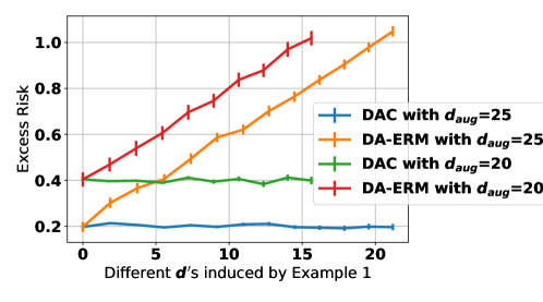
Example 2.
Consider a 30-dimensional linear regression. The original training set contains 50 samples. The inputs s are generated independently from and we set with and . The noise variance is set to . We partition into 3 parts and take the following augmentations: , where .
Notice that the augmentation perturbs and and leaving unchanged, we therefore have . By changing and , we can have different augmentations with different . The results for and various s are presented in Figure 4.1. The excess risks precisely match Theorem 4.1. It confirms that the DAC regularization is strictly better than DA-ERM for a wide variety of augmentations.
4.5 Beyond Label Invariant Augmentation
In this section, we extend our analysis to misspecified augmentations by relaxing the label invariance assumption (such that ). With an illustrative linear regression problem, we show that DAC also brings advantages over DA-ERM for misspecified augmentations.
We first recall the linear regression setup: given a set of i.i.d. samples that follows where are zero-mean independent noise with , we aim to learn the unknown ground truth . For randomly generated misspecified augmentations that alter the labels (i.e., ), a proper consistency constraint is (where is an augmentation of , noticing that corresponds to label invariant augmentations in Definition 4.1). For , the constrained optimization is equivalent to:
| (4.4) | ||||
for some finite . We compare to the solution learned with ERM on augmented data (as in Equation 4.3):
Let and . With , , and its reweighted analog , we further introduce positive semidefinite matrices: , , and . For demonstration purpose, we consider fixed and , with respect to which we introduce distortion factors as the minimum constants that satisfy and (notice that such exist almost surely when and are drawn from absolutely continuous marginal distributions).
Recall from Section 4.4. Let denote the rank- orthogonal projector onto . Then, for , we have the following result:
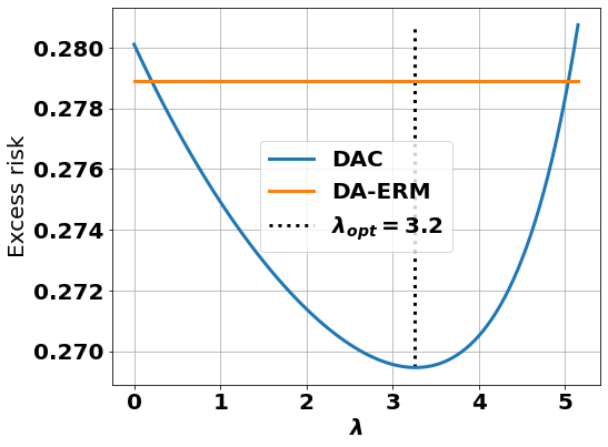
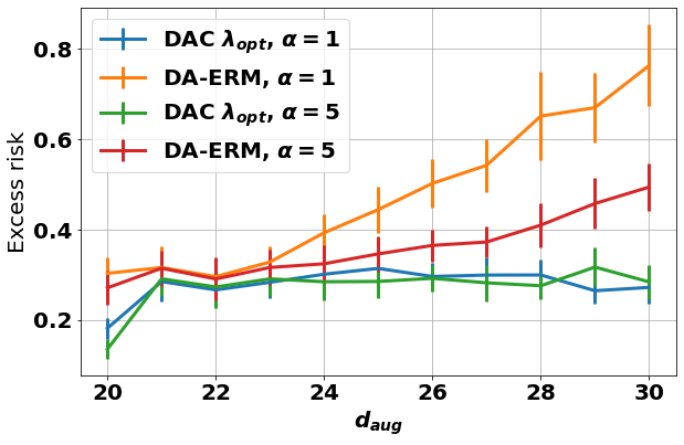
Theorem 4.2.
Learning with DAC regularization (Equation 4.4), we have that, at the optimal 222A positive (semi)definite matrix induces a (semi)norm: for all conformable .,
whereas learning with DA-ERM (Equation 4.3),
Here, measures the misspecification in by the augmentations .
One advantage of DAC regularization derives from its flexibility in choosing regularization parameter . With a proper (e.g., see Figure 4.2(a)) that matches the misspecification , DAC effectively reduces the function class from to and therefore improves the sample efficiency.
Another advantage of DAC is that, in contrast to DA-ERM, the consistency regularization term in Equation 4.4 refrains from learning the original labels with misspecified augmentations when a suitable is identified implicitly via . This allows DAC to learn from fewer but stronger (potentially more severely misspecified) augmentations (e.g., Figure 4.2(b)). Specifically, as , the excess risk of DAC with the optimal converges to zero by learning from unbiased labels , whereas DA-ERM suffers from a bias term due to the bias from misspecified augmentations.
Example 3.
As in Example 2, we consider a linear regression problem of dimension with misspecified augmentations on i.i.d. training samples drawn from . We aim to learn (where , ) under label noise . The misspecified augmentations mimic the effect of color jitter by adding i.i.d. Gaussian noise entry-wisely to the last feature coordinates: where for all , – such that with probability . The -th coordinates of are misspecified by the augmentations.
As previously discussed on Theorem 4.2, DAC is more robust than DA-ERM to misspecified augmentations, and therefore can learn with fewer (smaller ) and stronger (larger ) augmentations. In addition, DAC generally achieves better generalization than DA-ERM with limited samples.
4.6 Beyond Linear Model
In this section, we extend our analysis of DAC regularization to non-linear models, including the two-layer neural networks, and DNN-based classifiers with expansion-based augmentations.
Further, in addition to the popular in-distribution setting where we consider a unique distribution for both training and testing, DAC regularization is also known to improve out-of-distribution generalization for settings like domain adaptation. We defer detailed discussion on such advantage of DAC regularization for linear regression in the domain adaptation setting to Section B.4.
4.6.1 Two-layer Neural Network
We first generalize our analysis to an illustrative nonlinear model – two-layer ReLU network. With and , we consider a ground truth distribution induced by . For the unknown ground truth function , denotes the element-wisely ReLU function; consists of for all ; and is i.i.d. Gaussian noise. In terms of the function class , for some constant , let
such that . For regression, we again consider square loss and learn with DAC on the first layer: .
Let , and be the projector onto the null space of . Under mild regularity conditions (i.e., being sufficiently large, being subgaussian, and distribution of being absolutely continuous, as specified in Section B.2), regression over two-layer ReLU networks with the DAC regularization generalizes as following:
Theorem 4.3 (Informal result on two-layer neural network with DAC (formally in Theorem B.2)).
Conditioned on and , with and , for any , with probability at least over ,
Recall . With a sufficiently large (as specified in Section B.2), we have with high probability333Here we only account for the randomness in but not that in which characterizes for conciseness. We refer the readers to Section B.2 for a formal tail bound on .. Meanwhile, applying DA-ERM directly on the augmented samples achieves no better than , where the first term corresponds to the generalization bound for a -dimensional regression with i.i.d. samples (in contrast to augmented samples that are potentially dependent); and the second term follows as the augmentations keep a -dimensional subspace (i.e., the null space of ) intact, in which DA-ERM can only rely on the original samples for learning. In specific, the first term will dominate the with limited augmented data (i.e., being small).
Comparing the two, we see that DAC tends to be more efficient than DA-ERM, and such advantage is enhanced with strong but limited data augmentations (i.e., large and small ). For instance, with and , the generalization error of DA-ERM scales as , while DAC yields a dimension-free error.
As a synopsis for the regression cases in Section 4.4, Section 4.5, and Section 4.6.1 generally, the effect of DAC regularization can be casted as a dimension reduction by – dimension of the subspace perturbed by data augmentations where features contain scarce label information.
4.6.2 Classification with Expansion-based Augmentations
A natural generalization of the dimension reduction viewpoint on DAC regularization in the regression setting is the complexity reduction for general function classes. Here we demonstrate the power of DAC on function class reduction in a DNN-based classification setting.
Concretely, we consider a multi-class classification problem: given a probability space with marginal distribution and classes , let be the ground truth classifier, partitioning into disjoint sets such that . In the classification setting, we replace Definition 4.1 with the notion of expansion-based data augmentations introduced in [162, 22].
Definition 4.2 (Expansion-based augmentations (formally in Definition B.2)).
With respect to an augmentation function , let be the neighborhood of . For any , we say that induces -expansion-based data augmentations if (a) for all ; and (b) for all , given any with , .
Particularly, Definition 4.2(a) enforces that the ground truth classifier is invariant throughout each neighborhood. Meanwhile, the expansion factor in Definition 4.2(b) serves as a quantification of augmentation strength – a larger implies a stronger augmentation .
We aim to learn with loss from induced by the class of -layer fully connected neural networks with maximum width , where , , , and is the activation function.
Over a general probability space , DAC with expansion-based augmentations requires stronger conditions than merely consistent classification over for all labeled training samples . Instead, we enforce a large robust margin (adapted from [162], see Section B.3) over an finite set of unlabeled samples that is independent of and drawn i.i.d. from . Intuitively, measures the maximum allowed perturbation in all parameters of such that predictions remain consistent throughout (e.g., is equivalent to enforcing consistent classification outputs). For any , the DAC regularization reduces the function class to
Then for , we have the following.
Theorem 4.4 (Informal result on classification with DAC (formally in Theorem B.7)).
Given an augmentation function that induces -expansion-based data augmentations (Definition 4.2) such that
for any , with probability at least , we have such that
In particular, DAC regularization leverages the unlabeled samples and effectively decouples the labeled sample complexity from the complexity of the function class (characterized by and and encapsulated in ) via the reduced function class . Notably, Theorem 4.4 is reminiscent of [162] Theorem 3.6, 3.7, and [22] Theorem 2.1, 2.2, 2.3. We unified the existing theories under our function class reduction viewpoint to demonstrate its generality.
4.7 Experiments
In this section, we empirically verify that training with DAC learns more efficiently than DA-ERM. The dataset is derived from CIFAR-100, where we randomly select 10,000 labeled data as the training set (i.e., 100 labeled samples per class). During the training time, given a training batch, we generate augmentations by RandAugment [35]. We set the number of augmentations per sample to 7 unless otherwise mentioned.
The experiments focus on comparisons of 1) training with consistency regularization (DAC), and 2) empirical risk minimization on the augmented dataset (DA-ERM). We use the same network architecture (a WideResNet-28-2 [176]) and the same training settings (e.g., optimizer, learning rate schedule, etc) for both methods. We defer the detailed experiment settings to Section B.6. Our test set is the standard CIFAR-100 test set, and we report the average and standard deviation of the testing accuracy of 5 independent runs. The consistency regularizer is implemented as the distance of the model’s predictions on the original and augmented samples.
| DA-ERM | DAC Regularization | ||||
|---|---|---|---|---|---|
Efficacy of DAC regularization. We first show that the DAC regularization learns more efficiently than DA-ERM. The results are listed in Table 4.1. In practice, the augmentations almost always alter the label distribution, we therefore follow the discussion in section 4.5 and adopt a finite (i.e., the multiplicative coefficient before the DAC regularization, see Equation 4.1). With proper choice of , training with DAC significantly improves over DA-ERM.
| Number of Augmentations | 1 | 3 | 7 | 15 |
|---|---|---|---|---|
| DA-ERM | ||||
| DAC () |
| Number of Labeled Data | 1000 | 10000 | 20000 |
|---|---|---|---|
| DA-ERM | |||
| DAC () |
| No Augmentation | DA-ERM | DAC () | DAC () | DAC () |
|---|---|---|---|---|
| Number of Unlabeled Data | 5000 | 10000 | 20000 |
|---|---|---|---|
| FixMatch | 67.74 | 69.23 | 70.76 |
| FixMatch + DAC () | 71.24 | 72.7 | 74.04 |
DAC regularization helps more with limited augmentations. Our theoretical results suggest that the DAC regularization learns efficiently with a limited number of augmentations. While keeping the number of labeled samples to be 10,000, we evaluate the performance of the DAC regularization and DA-ERM with different numbers of augmentations. The number of augmentations for each training sample ranges from 1 to 15, and the results are listed in Table 4.2. The DAC regularization offers a more significant improvement when the number of augmentations is small. This clearly demonstrates that the DAC regularization learns more efficiently than DA-ERM.
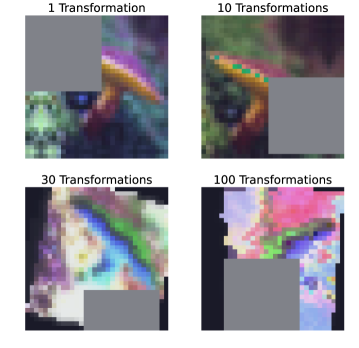
DAC regularization helps more when data is scarce. We conduct experiments with different numbers of labeled samples, ranging from 1,000 (i.e., 10 images per class) to 20,000 samples (i.e., 200 images per class). We generate 3 augmentations for each of the samples during the training time, and the results are presented in Table 4.3. Notice that the DAC regularization gives a bigger improvement over DA-ERM when the labeled samples are scarce. This matches the intuition that when there are sufficient training samples, data augmentation is less necessary. Therefore, the difference between different ways of utilizing the augmented samples becomes diminishing.
DAC performs well under misspecified augmentations. As suggested by Theorem 4.2, DAC is more robust to misspecified augmentations with proper . We further empirically verify this result with misspecified augmentations - where the augmentations are generated by applying 100 random transformations. When too many transformations are applied (see illustration in Figure 4.3), the augmentation will alter the label distribution and is thus misspecified. The results are presented in Table 4.4. Notice that with , the DAC delivers the best accuracy, which supports our theoretical results.
Further, comparing the results of Table 4.1 and Table 4.4, we see that the optimal is different when the augmentations are misspecified. Because of the flexibility in choosing , DAC is able to outperform DA-ERM, which matches the result in Theorem 4.2.
Combining with a semi-supervised learning algorithm. Here we show that the DAC regularization can be easily extended to the semi-supervised learning setting. We take the previously established semi-supervised learning method FixMatch [135] as the baseline and adapt the FixMatch by combining it with the DAC regularization. Specifically, besides using FixMatch to learn from the unlabeled data, we additionally generate augmentations for the labeled samples and apply DAC. In particular, we focus on the data-scarce regime by only keeping 10,000 labeled samples and at most 20,000 unlabeled samples. Results are listed in Table 4.5. We see that the DAC regularization also improves the performance of FixMatch when the unlabeled samples are scarce. This again demonstrates the efficiency of learning with DAC.
4.8 Conclusion
In this paper, we take a step toward understanding the statistical efficiency of DAC with limited data augmentations. At the core, DAC is statistically more efficient because it reduces problem dimensions by enforcing consistency regularization.
We demonstrate the benefits of DAC compared to DA-ERM (expanding training set with augmented samples) both theoretically and empirically. Theoretically, we show a strictly smaller generalization error under linear regression, and explicitly characterize the generalization upper bound for two-layer neural networks and expansion-based data augmentations. We further show that DAC better handles the label misspecification caused by strong augmentations. Empirically, we provide apples-to-apples comparisons between DAC and DA-ERM. These together demonstrate the superior efficacy of DAC over DA-ERM.
Chapter 5 Adaptively Weighted Data Augmentation Consistency Regularization: Application in Medical Image Segmentation
Abstract
Concept shift is a prevailing problem in natural tasks like medical image segmentation where samples usually come from different subpopulations with variant correlations between features and labels. One common type of concept shift in medical image segmentation is the “information imbalance” between label-sparse samples with few (if any) segmentation labels and label-dense samples with plentiful labeled pixels.
Existing distributionally robust algorithms have focused on adaptively truncating/down-weighting the “less informative” (i.e., label-sparse in our context) samples.
To exploit data features of label-sparse samples more efficiently, we propose an adaptively weighted online optimization algorithm — AdaWAC— to incorporate data augmentation consistency regularization in sample reweighting. Our method introduces a set of trainable weights to balance the supervised loss and unsupervised consistency regularization of each sample separately. At the saddle point of the underlying objective, the weights assign label-dense samples to the supervised loss and label-sparse samples to the unsupervised consistency regularization.
We provide a convergence guarantee by recasting the optimization as online mirror descent on a saddle point problem. Our empirical results demonstrate that AdaWAC not only enhances the segmentation performance and sample efficiency but also improves the robustness to concept shift on various medical image segmentation tasks with different UNet-style backbones.111This chapter is based on the following published conference paper:
\bibentrydong2022adawac [48].
5.1 Introduction
Modern machine learning is revolutionizing the field of medical imaging, especially in computer-aided diagnosis with computed tomography (CT) and magnetic resonance imaging (MRI) scans. However, classical learning objectives like empirical risk minimization (ERM) generally assume that training samples are independently and identically (i.i.d.) distributed, whereas real-world medical image data rarely satisfy this assumption. Figure 5.1 instantiates a common observation in medical image segmentation where the segmentation labels corresponding to different cross-sections of the human body tend to have distinct proportions of labeled (i.e., non-background) pixels, which is accurately reflected by the evaluation of supervised cross-entropy loss during training. We refer to this as the “information imbalance” among samples, as opposed to the well-studied “class imbalance” [164, 141, 174] among the numbers of segmentation labels in different classes. Such information imbalance induces distinct difficulty/paces of learning with the cross-entropy loss for different samples [159, 149, 142, 66]. Specifically, we say a sample is label-sparse when it contains very few (if any) segmentation labels; in contrast, a sample is label-dense when its segmentation labels are prolific. Motivated by the information imbalance among samples, we explore the following questions:
What is the effect of separation between sparse and dense labels on segmentation?
Can we leverage such information imbalance to improve the segmentation accuracy?
We formulate the mixture of label-sparse and label-dense samples as a concept shift — a type of distribution shift in the conditional distribution of labels given features . Coping with concept shifts, prior works have focused on adaptively truncating (hard-thresholding) the empirical loss associated with label-sparse samples. These include the Trimmed Loss Estimator [130], MKL-SGD [127], Ordered SGD [82], and the quantile-based Kacmarz algorithm [67]. Alternatively, another line of works [160, 122] proposes to relax the hard-thresholding operation to soft-thresholding by down-weighting instead of truncating the less informative samples. However, diminishing sample weights reduces the importance of both the features and the labels simultaneously, which is still not ideal as the potentially valuable information in the features of the label-sparse samples may not be fully used.
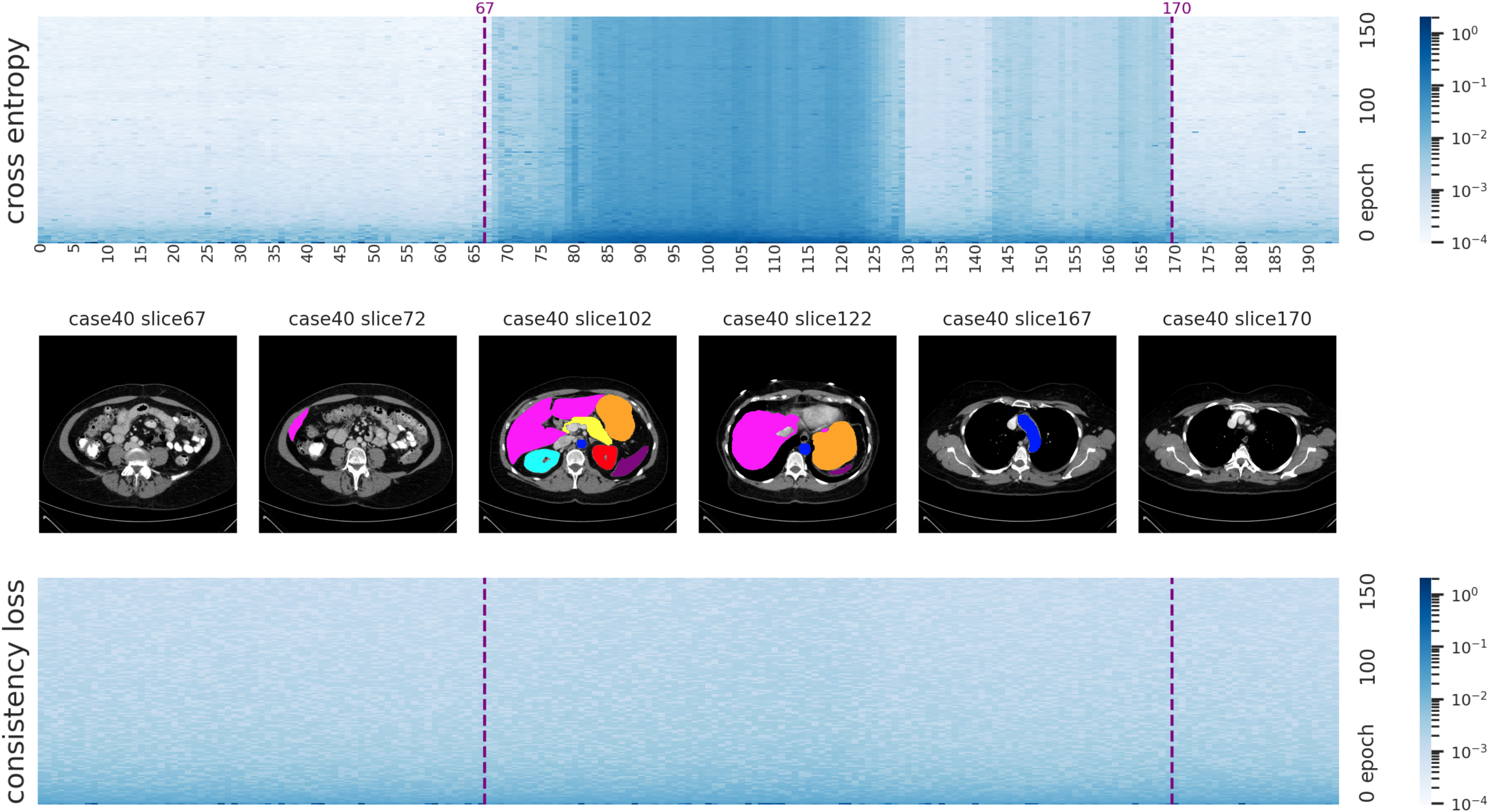
For further exploitation of the feature of training samples, we propose the incorporation of data augmentation consistency regularization on label-sparse samples. As a prevalent strategy for utilizing unlabeled data, consistency regularization [5, 88, 135] encourages data augmentations of the same samples to lie in the vicinity of each other on a proper manifold. For medical imaging segmentation, consistency regularization has been extensively studied in the semi-supervised learning setting [17, 179, 90, 158, 178, 181, 7] as a strategy for overcoming label scarcity. Nevertheless, unlike general vision tasks, for medical image segmentation, the scantiness of unlabeled image data can also be a problem due to regulations and privacy considerations [80], which makes it worthwhile to reminisce the more classical supervised learning setting. In contrast to the aforementioned semi-supervised strategies, we explore the potency of consistency regularization in the supervised learning setting by leveraging the information in the features of label-sparse samples via data augmentation consistency regularization.
To naturally distinguish the label-sparse and label-dense samples, we make a key observation that the unsupervised consistency regularization on encoder layer outputs (of a UNet-style architecture) is much more uniform across different subpopulations than the supervised cross-entropy loss (as exemplified in Figure 5.1). Since the consistency regularization is characterized by the marginal distribution of features but not labels, and therefore is less affected by the concept shift in , it serves as a natural reference for separating the label-sparse and label-dense samples. In light of this observation, we present the weighted data augmentation consistency (WAC) regularization — a minimax formulation that reweights the cross-entropy loss versus the consistency regularization associated with each sample via a set of trainable weights. At the saddle point of this minimax formulation, the WAC regularization automatically separates samples from different subpopulations by assigning all weights to the consistency regularization for label-sparse samples, and all weights to the cross-entropy terms for label-dense samples.
We further introduce an adaptively weighted online optimization algorithm — AdaWAC— for solving the minimax problem posed by the WAC regularization, which is inspired by a mirror-descent-based algorithm for distributionally robust optimization [122]. By adaptively learning the weights between the cross-entropy loss and consistency regularization of different samples, AdaWAC comes with both a convergence guarantee and empirical success.
The main contributions are summarized as follows:
-
•
We introduce the WAC regularization that leverages the consistency regularization on the encoder layer outputs (of a UNet-style architecture) as a natural reference to distinguish the label-sparse and label-dense samples (Section 5.3).
-
•
We propose an adaptively weighted online optimization algorithm — AdaWAC— for solving the WAC regularization problem with a convergence guarantee (Section 5.4).
-
•
Through extensive experiments on different medical image segmentation tasks with different UNet-style backbone architectures, we demonstrate the effectiveness of AdaWAC not only for enhancing the segmentation performance and sample efficiency but also for improving the robustness to concept shift (Section 5.5).
5.1.1 Related Work
Sample reweighting.
Sample reweighting is a popular strategy for dealing with distribution/subpopulation shifts in training data where different weights are assigned to samples from different subpopulations. In particular, the distributionally-robust optimization (DRO) framework [10, 53, 54, 122] considers a collection of training sample groups from different distributions. With the explicit grouping of samples, the goal is to minimize the worst-case loss over the groups. Without prior knowledge of sample grouping, importance sampling [110, 180, 2, 94, 60, 81], iterative trimming [82, 130], and empirical-loss-based reweighting [170] are commonly incorporated in the stochastic optimization process for adaptive reweighting and separation of samples from different subpopulations.
Data augmentation consistency regularization.
As a popular way of exploiting data augmentations, consistency regularization encourages models to learn the vicinity among augmentations of the same sample based on the assumption that data augmentations generally preserve the semantic information in data and therefore lie closely on proper manifolds. Beyond being a powerful building block in semi-supervised [5, 124, 88, 135, 12] and self-supervised [171, 70, 28, 63] learning, the incorporation of data augmentation and consistency regularization also provably improves generalization and feature learning even in the supervised learning setting [173, 129].
For medical imaging, data augmentation consistency regularization is generally leveraged as a semi-supervised learning tool [17, 179, 90, 158, 178, 181, 7]. In efforts to incorporate consistency regularization in segmentation tasks with augmentation-sensitive labels, [90] encourages transformation consistency between predictions with augmentations applied to the image inputs and the segmentation outputs. [7] penalizes inconsistent segmentation outputs between teacher-student models, with MixUp [177] applied to image inputs of the teacher model and segmentation outputs of the student model. Instead of enforcing consistency in the segmentation output space as above, we leverage the insensitivity of sparse labels to augmentations and encourage consistent encodings (in the latent space of encoder outputs) on label-sparse samples.
5.2 Problem Setup
Notation.
For any , we denote . We represent the elements and subtensors of an arbitrary tensor by adapting the syntax for Python slicing on the subscript (except counting from ). For example, denotes the -entry of the two-dimensional tensor , and denotes the -th row. Let be a function onto such that, for any event , if is true and otherwise. For any distribution and , we let denote the joint distribution of samples drawn i.i.d. from . Finally, we say that an event happens with high probability (w.h.p.) if the event takes place with probability .
5.2.1 Pixel-wise Classification with Sparse and Dense Labels
We consider medical image segmentation as a pixel-wise multi-class classification problem where we aim to learn a pixel-wise classifier that serves as a good approximation to the ground truth .
Recall the separation of cross-entropy losses between samples with different proportions of background pixels from Figure 5.1. We refer to a sample as label-sparse if most pixels in are labeled as background; for these samples, the cross-entropy loss on converges rapidly in the early stage of training. Otherwise, we say that is label-dense. Formally, we describe such variation as a concept shift in the data distribution.
Definition 5.1 (Mixture of label-sparse and label-dense subpopulations).
We assume that label-sparse and label-dense samples are drawn from and with distinct conditional distributions and but common marginal distribution such that (). For , we define as a data distribution where is drawn either from with probability or from with probability .
We aim to learn a pixel-wise classifier from a function class for all where the underlying function , parameterized by some , admits an encoder-decoder structure:
| (5.1) |
Here correspond to the encoder and decoder functions, respectively. The parameter space is equipped with the norm and its dual norm 222 For AdaWAC (Proposition 5.2 in Section 5.4), is simply a subspace in the Euclidean space with dimension equal to the total number of parameters for each , with and both being the -norm. . is a latent metric space.
To learn from segmentation labels, we consider the averaged cross-entropy loss:
| (5.2) | ||||
We assume the proper learning setting: there exists , which is invariant with respect to .333 We assume proper learning only to (i) highlight the invariance of the desired ground truth to that can be challenging to learn with finite samples in practice and (ii) provide a natural pivot for the convex and compact neighborhood of ground truth in 1 granted by the pretrained initialization, where can also be replaced with the pretrained initialization weights . In particular, neither our theory nor the AdaWAC algorithm requires the function class to be expressive enough to truly contain such .
5.2.2 Augmentation Consistency Regularization
Despite the invariance of to on the population loss, with a finite number of training samples in practice, the predominance of label-sparse samples would be problematic. As an extreme scenario for the pixel-wise classifier with encoder-decoder structure (Equation 5.1), when the label-sparse samples are predominant (), a decoder function that predicts every pixel as background can achieve near-optimal cross-entropy loss, regardless of the encoder function , considerably compromising the test performance (cf. Table 5.1). To encourage legit encoding even in the absence of sufficient dense labels, we leverage the unsupervised consistency regularization on the encoder function based on data augmentations.
Let be a distribution over transformations on where for any , each () induces an augmentation of that perturbs low-level information in . We aim to learn an encoder function that is capable of filtering out low-level information from and therefore provides similar encodings for augmentations of the same sample. Recalling the metric (e.g., the Euclidean distance) on , for a given scaling hyperparameter , we measure the similarity between augmentations with a consistency regularization term on : for any ,
| (5.3) |
For the training samples , we consider pairs of data augmentation transformations . In the basic version, we encourage the similar encoding of the augmentation pairs for all via consistency regularization:
| (5.4) |
We enforce consistency on in light of the encoder-decoder architecture: the encoder is generally designed to abstract essential information and filters out low-level non-semantic perturbations (e.g., those introduced by augmentations), while the decoder recovers the low-level information for the pixel-wise classification. Therefore, with different , the encoder output tends to be more consistent than the other intermediate layers, especially for label-dense samples.
5.3 Weighted Augmentation Consistency (WAC) Regularization
As the motivation, we begin with a key observation about the averaged cross-entropy:
Remark 5.1 (Separation of averaged cross-entropy loss on and ).
As demonstrated in Figure 5.1, the sparse labels from tend to be much easier to learn than the dense ones from , leading to considerable separation of averaged cross-entropy losses on the sparse and dense labels after a sufficient number of training epochs. In other words, for label-sparse samples and label-dense samples with high probability.
Although Equation 5.4 with consistency regularization alone can boost the segmentation accuracy during testing (cf. Table 5.4), it does not take the separation between label-sparse and label-dense samples into account. In Section 5.5, we will empirically demonstrate that proper exploitation of such separation, like the formulation introduced below, can lead to improved classification performance.
We formalize the notion of separation between and with the consistency regularization (Equation 5.3) as a reference in the following assumption 444 Although 1 may seem to be rather strong, it is only required for the separation guarantee of label-sparse and label-dense samples with high probability in Proposition 5.1, but not for the adaptive weighting algorithm introduced in Section 5.4 or in practice for the experiments. .
Assumption 1 (-separation between and ).
Given a sufficiently small , let be a compact and convex neighborhood of well-trained pixel-wise classifiers555With pretrained initialization, we assume that the optimization algorithm is always probing in .. We say that and are -separated over if there exists such that with probability over , the following hold:
-
(i)
for all given ;
-
(ii)
for all given .
This assumption is motivated by the empirical observation that the perturbation in induced by is more uniform across and than the averaged cross-entropy losses, as instantiated in Figure 5.3.
Under 1, up to a proper scaling hyperparameter , the consistency regularization (Equation 5.3) can separate the averaged cross-entropy loss (Equation 5.2) on label-sparse and label-dense samples with probability (as explained formally in Section C.1). In particular, the larger corresponds to the stronger separation between and .
With 1, we introduce a minimax formulation that incentivizes the separation of label-sparse and label-dense samples automatically by introducing a flexible weight that balances and for each of the samples.
| (5.5) | ||||
With convex and continuous loss and regularization terms (formally in Proposition 5.1), Equation 5.5 admits a saddle point corresponding to which separates the label-sparse and label-dense samples under 1.
Proposition 5.1 (Formal proof in Section C.1).
Assume that and are convex and continuous in for all and ; is compact and convex. If and are -separated (1), then there exists and such that
| (5.6) | ||||
Further, separates the label-sparse and label-dense samples——w.h.p..
That is, for samples drawn from a mixture of -separated and , the saddle point of in Equation 5.5 corresponds to on label-sparse samples (i.e., learning from the unsupervised consistency regularization), and on label-dense samples (i.e., learning from the supervised averaged cross-entropy loss).
Remark 5.2 (Connection to hard-thresholding algorithms).
The saddle point of Equation 5.5 is closely related to hard-thresholding algorithms like Ordered SGD [82] and iterative trimmed loss [130]. In each iteration, these algorithms update the model only on a proper subset of training samples based on the (ranking of) current empirical risks. Compared to hard-thresholding algorithms, (i) Equation 5.5additionally leverages the unused samples (e.g., label-sparse samples) for unsupervised consistency regularization on data augmentations; (ii) meanwhile, it does not require prior knowledge of the sample subpopulations (e.g., for ) which is essential for hard-thresholding algorithms.
Equation 5.5 further facilitates the more flexible optimization process. As we will empirically show in Table 5.2, despite the close relation between Equation 5.5 and the hard-thresholding algorithms (Remark 5.2), such updating strategies may be suboptimal for solving Equation 5.5.
5.4 Adaptively Weighted Augmentation Consistency (AdaWAC)
Inspired by the breakthrough made by [122] in the distributionally-robust optimization (DRO) setting where gradient updating on weights is shown to enjoy better convergence guarantees than hard thresholding, we introduce an adaptively weighted online optimization algorithm (Algorithm 6) for solving Equation 5.5 based on online mirror descent.
In contrast to the commonly used stochastic gradient descent (SGD), the flexibility of online mirror descent in choosing the associated norm space not only allows gradient updates on sample weights but also grants distinct learning dynamics to sample weights and model parameters , which leads to the following convergence guarantee.
Proposition 5.2 (Formally in Proposition C.1, proof in Section C.2, assumptions instantiated in Example 5).
Assume that and are convex and continuous in for all and . Assume moreover that is convex and compact. If there exist 666 Following the convention, we use in subscription to denote the dual spaces. For instance, recalling the parameter space characterized by the norm from Section 5.2.1, we use to denote its dual norm; while upper bound the dual norms of the gradients with respect to and . and such that
for all , , then with , Algorithm 6 provides
where and .
In addition to the convergence guarantee, Algorithm 6 also demonstrates superior performance over hard-thresholding algorithms for segmentation problems in practice (Table 5.2). An intuitive explanation is that instead of filtering out all the label-sparse samples via hard thresholding, the adaptive weighting allows the model to learn from some sparse labels at the early epochs, while smoothly down-weighting of these samples since learning sparse labels tends to be easier (Remark 5.1). With the learned model tested on a mixture of label-sparse and label-dense samples, learning sparse labels at the early stage is crucial for accurate segmentation.
5.5 Experiments
In this section, we investigate the proposed AdaWAC algorithm (Algorithm 6) on different medical image segmentation tasks with different UNet-style architectures. We first demonstrate the performance improvements brought by AdaWAC in terms of sample efficiency and robustness to concept shift (Table 5.1). Then, we verify the empirical advantage of AdaWAC compared to the closely related hard-thresholding algorithms as discussed in Remark 5.2 (Table 5.2). Our ablation study (Table 5.4) further illustrates the indispensability of both sample reweighting and consistency regularization, the deliberate combination of which leads to the superior performance of AdaWAC 777We release our code anonymously at https://anonymous.4open.science/r/adawac-F5F8..
Experiment setup.
We conduct experiments on two medical image segmentation tasks: abdominal CT segmentation for Synapse multi-organ dataset (Synapse)888https://www.synapse.org/#!Synapse:syn3193805/wiki/217789 and cine-MRI segmentation for Automated cardiac diagnosis challenge dataset (ACDC)999https://www.creatis.insa-lyon.fr/Challenge/acdc/, with two UNet-like architectures: TransUNet [26] and UNet [119] (deferred to Section C.5.1). For the main experiments with TransUNet in Section 5.5, we follow the official implementation in [26] and use ERM+SGD as the baseline. We evaluate segmentations with two standard metrics—the average Dice-similarity coefficient (DSC) and the average -percentile of Hausdorff distance (HD95). Dataset and implementation details are deferred to Section C.4. Given the sensitivity of medical image semantics to perturbations, our experiments only involve simple augmentations (i.e., rotation and mirroring) adapted from [26].
It is worth highlighting that, in addition to the information imbalance among samples caused by the concept shift discussed in this work, the pixel-wise class imbalance (e.g., the predominance of background pixels) is another well-investigated challenge for medical image segmentation, where coupling the dice loss [164, 141, 174] in the objective is a common remedy used in many state-of-the-art methods [26, 23]. The implementation of AdaWAC also leverages the dice loss to alleviate pixel-wise class imbalance. We defer the detailed discussion to Section C.3.
5.5.1 Segmentation Performance of AdaWAC with TransUNet
Segmentation on Synapse.
Figure 5.2 visualizes the segmentation predictions on Synapse test slices given by models trained via AdaWAC (ours) and via the baseline (ERM+SGD) with TransUNet [26]. We observe that AdaWAC provides more accurate predictions on the segmentation boundaries and captures small organs better than the baseline.

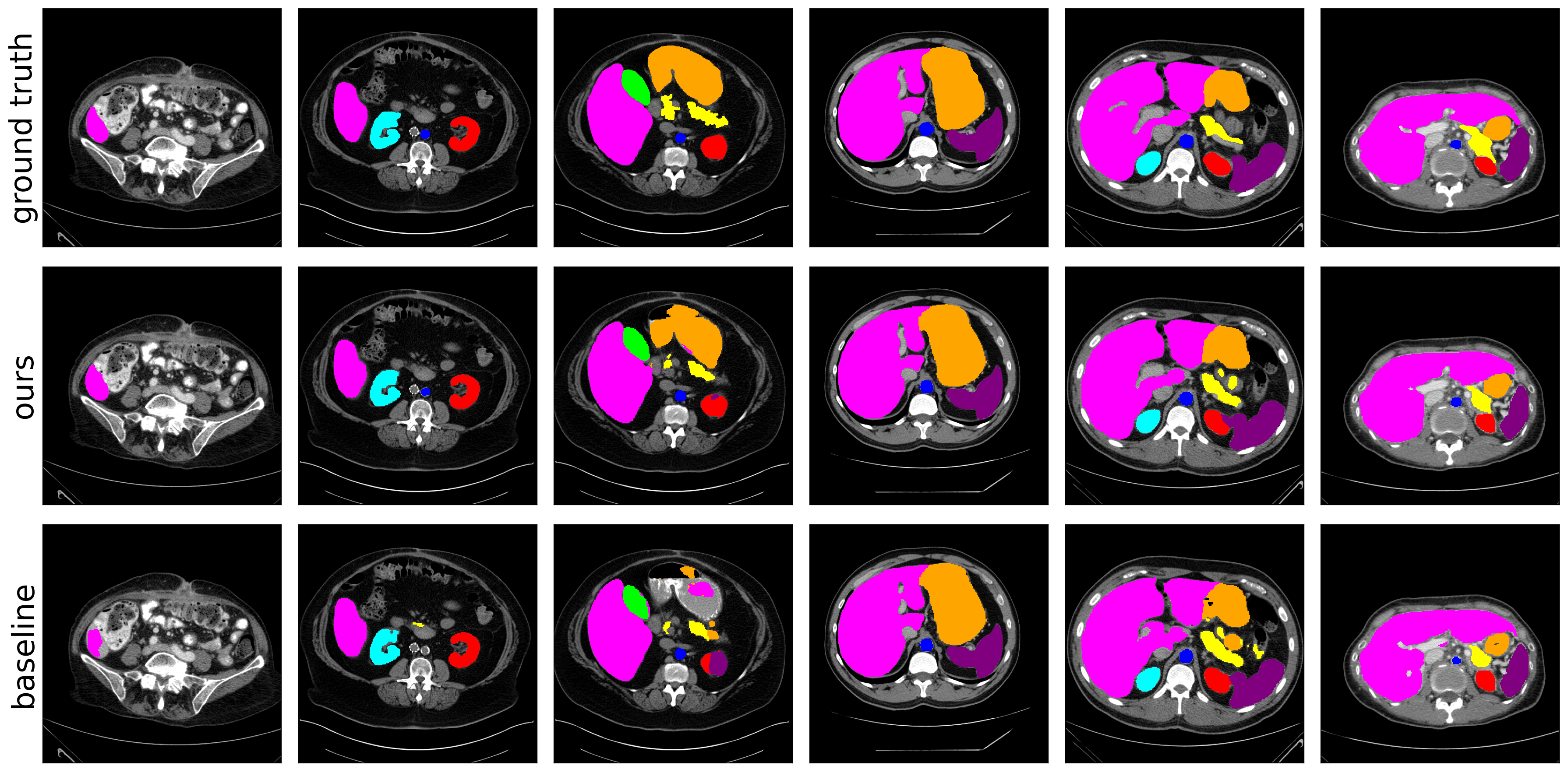
Visualization of AdaWAC.
As shown in Figure 5.3, with (Equation 5.2) of label-sparse versus label-dense slices weakly separated in the early epochs, the model further learns to distinguish of label-sparse/label-dense slices during training. By contrast, (Equation 5.3) remains mixed for all slices throughout the entire training process. As a result, the CE weights of label-sparse slices are much smaller than those of label-dense ones, pushing AdaWAC to learn more image representations but fewer pixel classifications for slices with sparse labels and learn more pixel classifications for slices with dense labels.
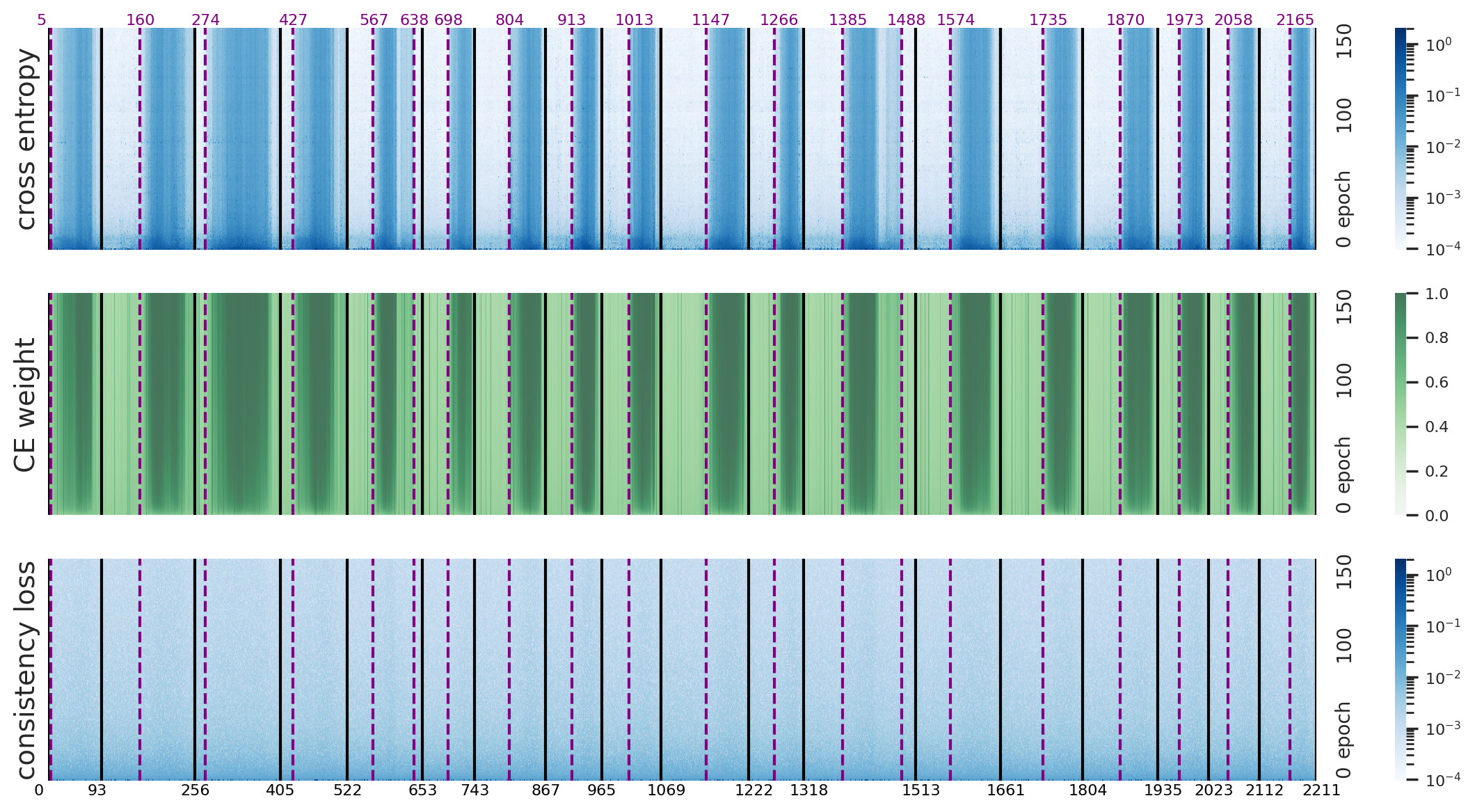
Sample efficiency and robustness.
We first demonstrate the sample efficiency of AdaWAC in comparison to the baseline (ERM+SGD) when training only on different subsets of the full Synapse training set (“full” in Table 5.1). Specifically, (i) half-slicecontains slices with even indices only in each case (patient)101010Such sampling is equivalent to doubling the time interval between two consecutive scans or halving the scanning frequency in practice, resulting in the halving of sample size.; (ii) half-volconsists of 9 cases uniformly sampled from the total 18 cases in full where different cases tend to have distinct s (i.e., ratios of label-dense samples); (iii) half-sparsetakes the first half slices in each case, most of which tend to be label-sparse (i.e., s are made to be small). As shown in Table 5.1, the model trained with AdaWAC on half-slice generalizes as well as a baseline model trained on full, if not better. Moreover, the half-vol and half-sparse experiments illustrate the robustness of AdaWAC to concept shift. Furthermore, such sample efficiency and distributional robustness of AdaWAC extend to the more widely used UNet architecture. We defer the detailed results and discussions on UNet to Section C.5.1.
Training Method DSC HD95 Aorta Gallbladder Kidney (L) Kidney (R) Liver Pancreas Spleen Stomach full baseline 76.66 0.88 29.23 1.90 87.06 55.90 81.95 75.58 94.29 56.30 86.05 76.17 AdaWAC 79.04 0.21 27.39 1.91 87.53 56.57 83.23 81.12 94.04 62.05 89.51 78.32 half-slice baseline 74.62 0.78 31.62 8.37 86.14 44.23 79.09 78.46 93.50 55.78 84.54 75.24 AdaWAC 77.37 0.40 29.56 1.09 86.89 55.96 82.15 78.63 94.34 57.36 86.60 77.05 half-vol baseline 71.08 0.90 46.83 2.91 84.38 46.71 78.19 74.55 92.02 48.03 76.28 68.47 AdaWAC 73.81 0.94 35.33 0.92 84.37 48.14 80.32 77.39 93.23 52.78 83.50 70.79 half-sparse baseline 31.74 2.78 69.72 1.37 65.71 8.33 59.46 51.59 51.18 10.72 6.92 0.00 AdaWAC 41.03 2.12 59.04 12.32 71.27 8.33 69.14 63.09 64.29 17.74 30.77 3.57
Comparison with hard-thresholding algorithms.
Table 5.2 illustrates the empirical advantage of AdaWAC over the hard-thresholding algorithms, as suggested in Remark 5.2. In particular, we consider the following hard-thresholding algorithms: (i) trim-trainlearns only from slices with at least one non-background pixel and trims the rest in each iteration on the fly; (ii) trim-ratioranks the cross-entropy loss in each iteration (mini-batch) and trims samples with the lowest cross-entropy losses at a fixed ratio – the ratio of all-background slices in the full training set (); (iii) ACRfurther incorporates the data augmentation consistency regularization directly via the addition of without reweighting; (iv) pseudo-AdaWACsimulates the sample weights at the saddle point and learns via on slices with at least one non-background pixel while via otherwise. We see that naive incorporation of ACR brings less observable boosts to the hard-thresholding methods. Therefore, the deliberate combination via reweighting in AdaWAC is essential for performance improvement.
Method baseline trim-train trim-ratio pseudo-AdaWAC AdaWAC +ACR +ACR DSC 76.66 0.88 76.80 1.13 78.42 0.17 76.49 0.16 77.71 0.56 77.72 0.65 79.04 0.21 HD95 29.23 1.90 32.05 2.34 27.84 1.16 31.96 2.60 28.51 2.66 28.45 1.18 27.39 1.91
Segmentation on ACDC.
Performance improvements granted by AdaWAC are also observed on the ACDC dataset (Table 5.3). We defer detailed visualization of ACDC segmentation to Section C.5.
Method DSC HD95 RV Myo LV TransUNet 89.40 0.22 2.55 0.37 89.17 83.24 95.78 AdaWAC (ours) 90.67 0.27 1.45 0.55 90.00 85.94 96.06
5.5.2 Ablation Study
On the influence of consistency regularization.
To illustrate the role of consistency regularization in AdaWAC, we consider the reweight-only scenario with such that and therefore (Algorithm 6 line 7) remains intact. With zero consistency regularization in AdaWAC, reweighting alone brings little improvement (Table 5.4).
On the influence of sample reweighting.
We then investigate the effect of sample reweighting under different reweighting learning rates (recall Algorithm 6): (i) ACR-onlyfor (equivalent to the naive addition of ), (ii) AdaWAC-0.01for , and (iii) AdaWAC-1.0for . As Table 5.4 implies, when removing reweighting from AdaWAC, augmentation consistency regularization alone improves DSC slightly from (baseline) to (ACR-only), whereas AdaWAC boosts DSC to (AdaWAC-1.0) with a proper choice of .
Method DSC HD95 Aorta Gallbladder Kidney (L) Kidney (R) Liver Pancreas Spleen Stomach baseline 76.66 0.88 29.23 1.90 87.06 55.90 81.95 75.58 94.29 56.30 86.05 76.17 reweight-only 76.91 0.88 30.92 2.37 87.18 52.89 82.15 77.11 94.15 58.35 86.36 77.08 ACR-only 78.01 0.62 27.78 2.80 87.51 58.79 83.39 79.26 94.70 58.99 86.02 75.43 AdaWAC-0.01 77.75 0.23 28.02 3.50 87.33 56.68 83.35 78.53 94.45 57.02 87.72 76.94 AdaWAC-1.0 79.04 0.21 27.39 1.91 87.53 56.57 83.23 81.12 94.04 62.05 89.51 78.32
5.6 Discussion
In this paper, we explore the information imbalance commonly observed in medical image segmentation and exploit the information in features of label-sparse samples via AdaWAC, an adaptively weighted online optimization algorithm. AdaWAC can be viewed as a careful combination of adaptive sample reweighting and data augmentation consistency regularization. By casting the information imbalance among samples as a concept shift in the data distribution, we leverage the unsupervised data augmentation consistency regularization on the encoder layer outputs (of UNet-style architectures) as a natural reference for distinguishing the label-sparse and label-dense samples via the comparisons against the supervised average cross-entropy loss. We formulate such comparisons as a weighted augmentation consistency (WAC) regularization problem and propose AdaWAC for iterative and smooth separation of samples from different subpopulations with a convergence guarantee. Our experiments on various medical image segmentation tasks with different UNet-style architectures empirically demonstrate the effectiveness of AdaWAC not only in improving the segmentation performance and sample efficiency but also in enhancing the distributional robustness to concept shifts.
Limitations and future directions.
From an algorithmic perspective, a limitation of this work is the utilization of the encoder layer outputs for data augmentation consistency regularization, which resulted in AdaWAC being specifically tailored to UNet-style backbones. However, our method can be generalized to other architectures in principle by selecting a representation extractor in the network that (i) well characterizes the marginal distribution of features (ii) while being robust to the concept shift in . Further investigation into such generalizations is a promising avenue for future research.
Meanwhile, noticing the prevalence of concept shifts in natural data, especially for dense prediction tasks like segmentation and detection, we hope to extend the application/idea of AdaWAC beyond medical image segmentation as a potential future direction.
Appendices
Chapter A Appendix for Chapter 3
A.1 Technical Lemmas
Lemma A.1.
Let be a random vector with , , and 111In the case where is rank-deficient, we slightly abuse the notation such that and refer to the respective pseudo-inverses. being -subgaussian222A random vector is -subgaussian if for any unit vector , is -subgaussian, for all .. Given a set of i.i.d. samples of , , and a set of weights corresponding to the samples, , let . If , then with probability at least ,
Concretely, with , , and , with high probability (at least ).
Proof.
We first denote as the orthogonal projector onto the subspace supported by the distribution of . With the assumptions and , we observe that and . Given the sample set of size for any , we let
Then the problem can be reduced to showing that, for any , with probability at least , . For this, we leverage the -net argument as follows.
For an arbitrary , we have
where, given being -subgaussian, is -subgaussian. Since
we know that is -subexponential333We abbreviate -subexponential (i.e., recall that a random variable is -subexponential if for all ) simply as -subexponential.. With for all such that , we recall Bernstein’s inequality [151, Theorem 2.8.2][154, Section 2.1.3],
where and .
Let be an -net such that . Then for some , by the union bound,
whenever where .
Now for any , there exists some such that . Therefore,
Taking the supremum over , with probability at least ,
With , we have .
Overall, if , then with probability at least , we have .
As a concrete instance, when and , by taking , we have with high probability (at least where ). ∎
Lemma A.2 (Cauchy interlacing theorem).
Given an arbitrary matrix and an orthogonal projection with orthonormal columns, for all ,
Proof of Lemma A.2.
Lemma A.3 ([75] (7.3.14)).
For arbitrary matrices ,
| (A.1) |
for all , such that .
Lemma A.4 ([[75] (7.3.13)).
For arbitrary matrices ,
| (A.2) |
for all , such that .
A.2 Supplementary Experiments
A.2.1 Upper and Lower Space-agnostic Bounds
In this section, we visualize and compare the upper and lower bounds in Theorem 3.1 under the sufficient multiplicative oversampling regime (i.e., . Recall that where is the target rank, is the oversampled rank, and is the full rank of the matrix ).
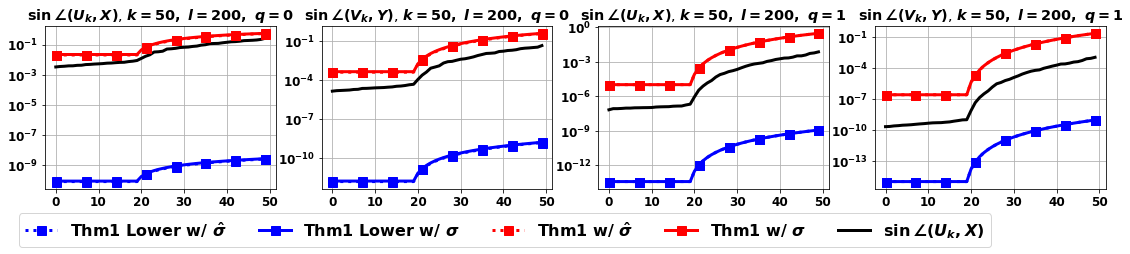
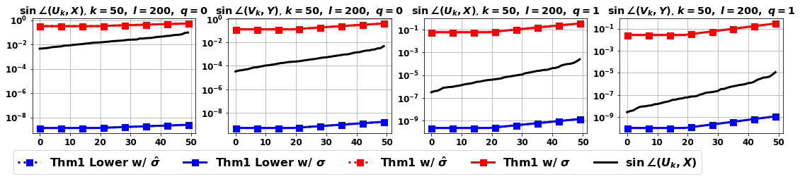
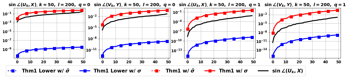
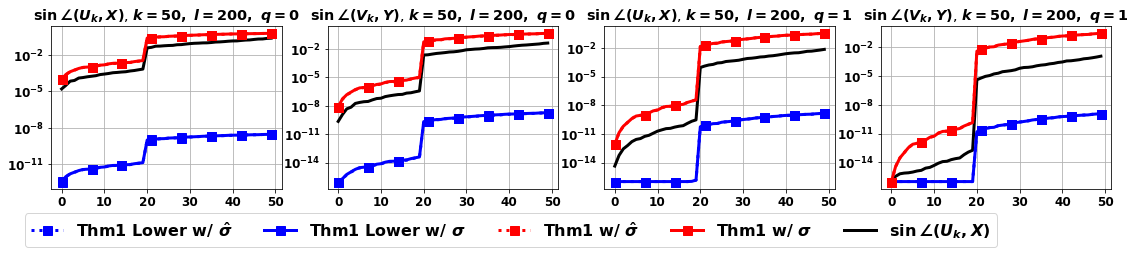
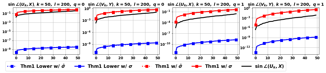
With the same set of target matrices described in Section 3.6.1, from Figure A.1 to Figure A.5,
-
1.
Red lines and dashes represent the upper bounds in Equation 3.2 and Equation 3.2 evaluated with the true (lines) and approximated (dashes) singular values, , and , respectively, where we simply ignore tail decay and suppress constants for the distortion factors and set
-
2.
Blue lines and dashes present the lower bounds in Equation 3.4 and Equation 3.5 evaluated with and , respectively, and slightly larger constants associated with the distortion factors
The numerical observations imply that the empirical validity of lower bounds requires more aggressive oversampling than that of upper bounds. In particular, we recall from Section 3.6.2 that is usually sufficient for the upper bounds to hold numerically. In contrast, the lower bounds generally require at least , with slightly larger constants associated with the distortion factors and .
Chapter B Appendix for Chapter 4
B.1 Linear Regression Models
In this section, we present formal proofs for the results on linear regression in the fixed design where the training samples and their augmentations are considered to be fixed. We discuss two types of augmentations: the label invariant augmentations in Section 4.4 and the misspecified augmentations in Section 4.5.
B.1.1 Linear Regression with Label Invariant Augmentations
For fixed , let in this section. We recall that since there is no randomness in in fix design setting. Assuming that admits full column rank, we have the following theorem on the excess risk of DAC and ERM:
Theorem B.1 (Formal restatement of Theorem 4.1 on linear regression.).
Learning with DAC regularization, we have , while learning with ERM directly on the augmented dataset, we have . is defined as
where with and is the orthogonal projector onto .
Proof.
With , the excess risk of ERM on the augmented training set satisfies that:
Let and denote the column space of and , respectively. Notice that is a subspace of both and . Observing that , we have
By the data augmentation consistency constraint, we are essentially solving the linear regression on the -dimensional space . The rest of proof is identical to standard regression analysis, with features first projected to :
∎
B.1.2 Linear Regression Beyond Label Invariant Augmentations
Proof of Theorem 4.2.
With , we start by partitioning the excess risk into two parts – the variance from label noise and the bias from feature-label mismatch due to augmentations (i.e., ):
First, we consider learning with DAC regularization with some finite ,
By setting the gradient of Equation 4.4 with respect to to 0, with , we have
Then with ,
For the variance term, we have
For the semi-positive definite matrix , we introduce the spectral decomposition:
where consists of orthonormal columns and . Then
For the bias term, we observe that
Then with , we have
To simply the optimization of regularization parameter , we leverage upper bounds of the variance and bias terms:
Then with , we have the generalization bound for in Theorem 4.2.
Second, we consider learning with DA-ERM:
With
we again partition the excess risk into the variance and bias terms. For the variance term, with the assumptions and , we have
Additionally, for the bias term, we have
Combining the variance and bias leads to the generalization bound for in Theorem 4.2. ∎
B.2 Two-layer Neural Network Regression
In the two-layer neural network regression setting with described in Section 4.6.1, let be a set of i.i.d. samples drawn from the marginal distribution that satifies the following.
Assumption 2 (Regularity of marginal distribution).
Let be zero-mean , with covairance matrix whose eigenvalues are bounded by constant factors , such that is -subgaussian 111A random vector is -subgaussian if for any unit vector , is -subgaussian, ..
For the sake of analysis, we isolate the augmented part in and denote the set of these augmentations as
where for each sample , is a set of augmentations generated from , and is the vertical stack of identity matrices. Analogous to the notions with respect to in the linear regression cases in Section B.1, in this section, we denote and quantify the augmentation strength as
such that can be intuitively interpreted as the number of dimensions in the span of the unlabeled samples, , perturbed by the augmentations.
Then, to learn the ground truth distribution where , training with the DAC regularization can be formulated explicitly as
For the resulted minimizer , we have the following.
Theorem B.2 (Formal restatement of Theorem 4.3 on two-layer neural network with DAC).
Under 2, we suppose and satisfy that (a) ; and (b) admits an absolutely continuous distribution. Then conditioned on and , with and for some , for all , with probability at least (over ),
Moreover, to account for randomness in and , we introduce the following notion of augmentation strength.
Definition B.1 (Augmentation strength).
For any , let
Intuitively, the augmentation strength ensures that the feature subspace perturbed by the augmentations in has a minimum dimension with probability at least . A larger corresponds to stronger augmentations. For instance, when almost surely (e.g., when the augmentations are identical copies of the original samples, corresponding to the weakest augmentation – no augmentations at all), we have for all . Whereas for randomly generated augmentations, is likely to be larger (i.e., with more dimensions being perturbed). For example in Example 3, for a given , with random augmentations where for all , , we have with probability . That is for all .
Leveraging the notion of augmentation strength in Definition B.1, we show that the stronger augmentations lead to the better generalization by reducing in Theorem B.2.
Corollary B.3.
When and , for any , with probability at least (over and ), we have .
To prove Theorem B.2, we start by showing that, with sufficient samples (), consistency of the first layer outputs over the samples implies consistency of those over the population.
Lemma B.4.
Under the assumptions in Theorem B.2, every size- subset of rows in is linearly independent almost surely.
Proof of Lemma B.4.
Since , it is sufficient to show that a random matrix with an absolutely continuous distribution is totally invertible 222A matrix is totally invertible if all its square submatrices are invertible. almost surely.
It is known that for any dimension , an square matrix is singular if where entries of lie within the roots of the polynomial equation specified by the determinant. Therefore, the set of all singular matrices in has Lebesgue measure zero,
Then, for an absolutely continuous probability measure with respect to , we also have
Since a general matrix contains only finite number of submatrices, when is drawn from an absolutely continuous distribution, by the union bound, . That is, is totally invertible almost surely. ∎
Lemma B.5.
Under the assumptions in Theorem B.2, the hidden layer in the two-layer ReLU network learns , the invariant subspace under data augmentations : with high probability,
Proof of Lemma B.5.
We will show that for all , , with high probability, which then implies that given any , for all .
For any associated with an arbitrary fixed , let be the inclusion-wisely maximum row subset of such that element-wisely. Meanwhile, we denote as the augmentation of where is the vertical stack of identity matrices with size . Then the DAC constraint implies that .
Leveraging the assumptions in Theorem B.2, implies that . Therefore by Lemma B.4, with probability . Thus, enforces that . ∎
Proof of Theorem B.2.
Conditioned on and , we are interested in the excess risk with randomness on .
We first recall that Lemma B.5 implies where
Leveraging Equation (21) and (22) in [52], since is feasible under the constraint, by the basic inequality,
| (B.1) |
Knowing that with , we can rewrite Equation B.1 as
First, we observe that measures the empirical Gaussian width of over . Moreover, by observing that for any and ,
and
we know that the function is -Lipschitz in norm. Therefore, by [155] Theorem 2.26, we have that with probability at least ,
where the empirical Gaussian complexity is upper bounded by
∎
Proof of Corollary B.3.
By Definition B.1, we have with probability at least that and . Meanwhile, leveraging Lemma B.12, we have that under 2 and with , with high probability,
Therefore, there exists with such that, with probability at least ,
∎
B.3 Classification with Expansion-based Augmentations
We first recall the multi-class classification problem setup in Section 4.6.2, while introducing some helpful notions. For an arbitrary set , let , and be the ground truth classifier that partitions : for each , let , with . In addition, for an arbitrary classifier , we denote the majority label with respect to for each class,
along with the respective class-wise local and global minority sets,
Given the marginal distribution , we introduce the expansion-based data augmentations that concretizes Definition 4.1 in the classification setting:
Definition B.2 (Expansion-based data augmentations, [22]).
We call an augmentation function that induces expansion-based data augmentations if is class invariant: for all . Let
be the neighborhoods of and with respect to . Then, satisfies
-
(a)
-constant expansion if given any with and for all , ;
-
(b)
-multiplicative expansion if for all , given any with , .
On Definition B.2, we first point out that the ground truth classifier is invariant throughout the neighborhood: given any , for all . Second, in contrast to the linear regression and two-layer neural network cases where we assume , with the expansion-based data augmentation over a general , the notion of in Definition B.1 is not well-established. Alternatively, we leverage the concept of constant / multiplicative expansion from [22], and quantify the augmentation strength with parameters or . Intuitively, the strength of expansion-based data augmentations is characterized by expansion capability of : for a neighborhood of proper size (characterized by or under measure ), the stronger augmentation leads to more expansion in , and therefore larger or . For example in Definition 4.2, we use an expansion-based augmentation function that satisfies -multiplicative expansion.
Adapting the existing setting in [162, 22], we concretize the classifier class with a function class of fully connected neural networks such that . To constrain the feasible hypothesis class through the DAC regularization with finite unlabeled samples, we recall the notion of all-layer-margin, (from [162]) that measures the maximum possible perturbation in all layers of while maintaining the prediction . Precisely, given any such that for some activation function and parameters , we can write where for all and for . For an arbitrary set of perturbation vectors such that for all , let be the perturbed neural network defined recursively such that
The all-layer-margin measures the minimum norm of the perturbation such that fails to provide the classification ,
| (B.2) |
With the notion of all-layer-margin established, for any that satisfies conditions in Definition B.2, the robust margin is defined as
Intuitively, the robust margin measures the maximum possible perturbation in all-layer weights of such that predictions on all data augmentations of remain consistent. For instance, is equivalent to enforcing for all .
To achieve finite sample guarantees, DAC regularization requires stronger consistency conditions than merely consistent classification outputs (i.e., ). Instead, we enforce for any 333The upper bound on ensures the proper learning setting, i.e., there exists such that for all . over an finite set of unlabeled samples that is independent of and drawn i.i.d. from . Then, learning the classifier with zero-one loss from a class of -layer fully connected neural networks with maximum width ,
where for all , and , we solve
| (B.3) | ||||
for any . The corresponding reduced function class is given by
Specifically, with , [162, 22] demonstrate the following for :
Proposition B.6 ([162] Theorem 3.7, [22] Proposition 2.2).
For any , with probability at least (over ),
where hides polylogarithmic factors in and .
Leveraging the existing theory above on finite sample guarantee of the maximum possible inconsistency, we have the following.
Theorem B.7 (Formal restatement of Theorem 4.4 on classification with DAC).
Learning the classifier with DAC regularization in Equation B.3 provides that, for any , with probability at least ,
| (B.4) |
where with defined in Proposition B.6, for any and ,
-
(a)
when satisfies -constant expansion, ;
-
(b)
when satisfies -multiplicative expansion, .
First, to quantify the function class complexity and relate it to the generalization error, we leverage the notion of Rademacher complexity and the associated standard generalization bound.
Lemma B.8.
Given a fixed function class (i.e., conditioned on ) and a -bounded and -Lipschitz loss function , let , , and . Then for any , with probability at least over ,
Proof of Lemma B.8.
We first decompose the expected excess risk as
where by the basic inequality. Since both , we then have
Let and . Then,
We will derive a tail bound for with the standard inequalities and symmetrization argument [155, 6], while the analogous statement holds for .
Let be a sample set generated by replacing an arbitrary sample in with an independent sample . Since is -bounded, we have . Then, via McDiarmid’s inequality [6],
For an arbitrary sample set , let be the empirical risk of with respect to . Then, by a classical symmetrization argument (e.g., proof of [155] Theorem 4.10), we can bound the expectation: for an independent sample set drawn i.i.d. from ,
Since are drawn i.i.d. from , we can introduce i.i.d. Rademacher random variables (independent of both and ) such that
where is the loss function class, and
denotes the Rademacher complexity. Analogously, . Therefore, assuming that holds, with probability at least ,
Finally, since is -Lipschitz for all , by [89] Theorem 4.12, we have . ∎
Lemma B.9 ([22], Lemma A.1).
For any , when satisfies
-
(a)
-constant expansion with , ;
-
(b)
-multiplicative expansion with , .
Proof of Lemma B.9.
We start with the proof for Lemma B.9 (a). By definition of and , we know that . Therefore, for any , one of the following two cases holds:
-
(i)
;
-
(ii)
. Since for all holds by construction, with the -constant expansion, .
Meanwhile, since the ground truth classifier is invariant throughout the neighborhoods, for , and therefore with each disjoint. Then, we observe that for each , here exists some such that . implies that , while suggests that there exists some where such that either and for , or and for . Therefore, we have
Moreover, since , we know that
That is, .
Overall, we have .
Proof of Theorem B.7.
To show Equation B.4, we leverage Lemma B.8 and observe that with the zero-one loss. Therefore, conditioned on (which depends only on but not on ), for any , with probability at least ,
For the upper bounds of the Rademacher complexity, let where denotes the global minority set with respect to . Lemma B.9 suggests that
-
(a)
when satisfies -constant expansion for some , ; while
-
(b)
when satisfies -multiplicative expansion for some , .
Then, it is sufficient to show that, conditioned on ,
| (B.5) |
To show this, we first consider a fixed set of observations in , . Let the number of distinct behaviors over in be
Then, by the Massart’s finite lemma, the empirical rademacher complexity with respect to is upper bounded by
By the concavity of , we know that,
| (B.6) |
Since for all , we have that, conditioned on ,
Plugging this into Section B.3 yields Equation B.5. Finally, the randomness in is quantified by , and upper bounded by Proposition B.6. ∎
B.4 Supplementary Application: Domain Adaptation
As a supplementary example, we demonstrate the possible failure of DA-ERM, and alternatively how DAC regularization can serve as a remedy. Concretely, we consider an illustrative linear regression problem in the domain adaptation setting: with training samples drawn from a source distribution and generalization (in terms of excess risk) evaluated over a related but different target distribution . With distinct and , we assume the existence of an unknown but unique inclusionwisely maximal invariant feature subspace such that , we aim to demonstrate the advantage of the DAC regularization over the ERM on augmented training set, with a provable separation in the respective excess risks.
Source and target distributions.
Formally, the source and target distributions are concretized with the causal graph in Figure B.1. For both and , the observable feature is described via a linear generative model in terms of two latent features, the ‘invariant’ feature and the ‘environmental’ feature :
where () consists of orthonormal columns. Let the label depends only on the invariant feature for both domains,
for some such that , while the environmental feature is conditioned on , , (along with the Gaussian noise ), and varies across different domains with . In other words, with the square loss , the optimal hypotheses that minimize the expected excess risk over the source and target distributions are distinct. Therefore, learning via the ERM with training samples from can overfit the source distribution, in which scenario identifying the invariant feature subspace becomes indispensable for achieving good generalization in the target domain.
For and , we assume the following regularity conditions:
Assumption 3 (Regularity conditions for and ).
Let satisfy 2. While satisfies that , and
-
(a)
for the invariant feature, for some ;
-
(b)
for the environmental feature, for some , and .
Training samples and data augmentations.
Let be a set of samples drawn i.i.d. from such that where . Recall that we denote the augmented training sets, including/excluding the original samples, respectively, with
In particular, we consider a set of augmentations that only perturb the environmental feature , while keep the invariant feature intact:
| (B.7) |
We recall the notion such that (), and assume that and are representative enough:
Assumption 4 (Diversity of and ).
is sufficiently large with , , and .
Excess risks in target domain.
Learning from the linear hypothesis class , with the DAC regularization on , we have
while with the ERM on augmented training set,
where and denote the vertical stacks of and identity matrices of size , respectively as denoted earlier.
We are interested in the excess risk on : where .
Theorem B.10 (Domain adaptation with DAC).
Theorem B.11 (Domain adaptation with ERM on augmented samples).
Proofs and instantiation.
Recall that for , denotes the orthogonal projector onto the dimension- null space of . Furthermore, let and be the orthogonal projectors onto the invariant and environmental feature subspaces, respectively, such that for all .
Proof of Theorem B.10.
By construction Equation B.7, , and it follows that . Meanwhile from 4, implies that . Therefore, , and the data augmentation consistency constraints can be restated as
Then with from 4,
where . Since , we have . Therefore, let , with high probability,
∎
Proof of Theorem B.11.
Let . Then with from 4, we have . Since , . Then, the ERM on the augmented training set yields
Meanwhile with from 3, we have . Therefore, by recalling that ,
such that the expected excess risk can be expressed as
where let ,
We denote
and observe that
Finally, we complete the proof by partitioning the lower bound for the target expected excess risk of into the invariantand environmental parts such that
∎
Now we construct a specific domain adaptation example with a large separation (i.e., proportional to ) in the target excess risk between learning with the DAC regularization (i.e., ) and with the ERM on augmented training set (i.e., ).
Example 4.
We consider and that follow the same set of relations in Figure B.1, except for the distributions over where . Precisely, let the environmental feature depend on :
where for and for , (recall from 3). Assume that the training set is sufficiently large, for some given . Augmenting with a simple by common type of data augmentations – the linear transforms, we let
and define
where and refer to the minimum and maximum singular values, respectively. Then under 3 and 4, with constant probability,
Proof of Example 4.
With the specified distribution, for ,
By Lemma B.12, under 3 and 4, we have that with high probability, . Therefore with and being independent,
and the rest follows from Theorem B.11. ∎
B.5 Technical Lemmas
Lemma B.12.
We consider a random vector with , , and 444In the case where is rank-deficient, we slightly abuse the notation such that and refer to the respective pseudo-inverses. being -subgaussian. Given an i.i.d. sample of , , for any , if , then with high probability.
Proof.
We first denote as the orthogonal projector onto the subspace supported by the distribution of . With the assumptions and , we observe that and . Given the sample set of size for some , we let . Then the problem can be reduced to showing that, with probability at least , . For this, we leverage the -net argument as following.
For an arbitrary , we have
where, given being -subgaussian, is -subgaussian. Since
we know that is -subexponential. Then, we recall the Bernstein’s inequality,
Let be an -net such that . Then for some , by the union bound,
whenever . By taking , we have that with high probability when , and taking is sufficient.
Now for any , there exists some such that . Therefore,
Taking the supremum over , with probability at least ,
With and , we have .
Overall, if , then with high probability, we have . ∎
Lemma B.13.
Let be an arbitrary subspace in , and be a Gaussian random vector. Then for any continuous and -Lipschitz function (i.e., for all ),
where acts on entry-wisely, . In other words, the Gaussian width of the image set is upper bounded by that of scaled by the Lipschitz constant.
Proof.
∎
B.6 Experiment Details
In this section, we provide the details of our experiments. Our code is adapted from the publicly released repo: https://github.com/kekmodel/FixMatch-pytorch.
Dataset: Our training dataset is derived from CIFAR-100, where the original dataset contains 50,000 training samples of 100 different classes. Out of the original 50,000 samples, we randomly select 10,000 labeled data as training set (i.e., 100 labeled samples per class). To see the impact of different training samples, we also trained our model with dataset that contains 1,000 and 20,000 samples. Evaluations are done on standard test set of CIFAR-100, which contains 10,000 testing samples.
Data Augmentation: During the training time, given a training batch, we generate corresponding augmented samples by RandAugment [35]. We set the number of augmentations per sample to 7, unless otherwise mentioned.
To generate an augmented image, the RandAugment draws transformations uniformaly at random from 14 different augmentations, namely {identity, autoContrast, equalize, rotate, solarize, color, posterize, contrast, brightness, sharpness, shear-x, shear-y, translate-x, translate-y}. The RandAugment provides each transformation with a single scalar (1 to 10) to control the strength of each of them, which we always set to 10 for all transformations. By default, we set (i.e., using 2 random transformations to generate an augmented sample). To see the impact of different augmentation strength, we choose . Examples of augmented samples are shown in Figure 4.3.
Parameter Setting: The batch size is set to 64 and the entire training process takes steps. During the training, we adopt the SGD optimizer with momentum set to 0.9, with learning rate for step being .
Additional Settings for the semi-supervised learning results: For the results on semi-supervised learning, besides the 10,000 labeled samples, we also draw additionally samples (ranging from 5,000 to 20,000) from the training set of the original CIFAR-100. We remove the labels of those additionally sampled images, as they serve as “unlabeled" samples in the semi-supervised learning setting. The FixMatch implementation follows the publicly available on in https://github.com/kekmodel/FixMatch-pytorch.
Chapter C Appendix for Chapter 5
C.1 Separation of Label-sparse and Label-dense Samples
Proof of Proposition 5.1.
We first observe that, since and are convex and continuous in for all and , for all , is continuous, convex in , and affine (thus concave) in ; and therefore so is . Then with the compact and convex domains and , Sion’s minimax theorem [134] suggests the minimax equality,
| (C.1) |
where can be replaced by respectively due to compactness of the domains.
Further, by the continuity and convexity-concavity of , the pointwise maximum is lower semi-continuous and convex in while the pointwise minimum is upper semi-continuous and concave in . Then via Weierstrass’ theorem ([14], Proposition 3.2.1), there exist and that achieve the minimax optimal by minimizing and maximizing . Along with Equation C.1, such provides a saddle point for Equation 5.5 ([14], Proposition 3.4.1).
Next, we show via contradiction that there exists a saddle point with attained on a vertex . Suppose the opposite, then for any saddle point , there must be an with , where we have the following contradictions:
-
(i)
If , decreasing to leads to , contradicting Equation 5.6.
-
(ii)
If , increasing to again leads to , contradicting Equation 5.6.
-
(iii)
If , can be replaced with any value in , including .
Therefore, there must be a saddle point with such that
Finally, it remains to show that w.h.p. over and ,
-
(i)
for all ; and
-
(ii)
for all ;
which leads to w.h.p. as desired. To illustrate this, we begin by observing that when and are -separated (1), since , there exists some such that for each ,
and
Therefore by the union bound over the set of samples ,
| (C.2) |
and
| (C.3) |
Applying the union bound again on Equation C.2 and Equation C.3, we have the desired condition holds with probability , i.e., w.h.p.. ∎
C.2 Convergence of AdaWAC
Recall the underlying function class parameterized by some that we aim to learn for the pixel-wise classifier , :
| (C.4) |
where correspond to the encoder and decoder functions. Formally, we consider an inner product space of parameters with the induced norm and dual norm .
For any , let . Then Equation 5.5 can be reformulated as:
| (C.5) | ||||
Proposition C.1 (Convergence (formal restatement of Proposition 5.2)).
Assume that and are convex and continuous in for all and , and that is convex and compact. If there exist
-
(i)
such that for all , and
-
(ii)
such that for all ,
then with , Algorithm 6 provides the convergence guarantee for the duality gap :
where and .
Proof of Proposition C.1.
The proof is an application of the standard convergence guarantee for the online mirror descent on saddle point problems, as recapitulated in Lemma C.2.
Specifically, for , we use the norm with its dual norm . We consider a mirror map such that . We observe that, since for all ,
and therefore is -strongly convex with respect to . With such , we have the associated Fenchel dual , along with the gradients
such that the mirror descent update on is given by
For uniformly, the stochastic gradient with respect to satisfies
Further, in the distance induced by , we have
Meanwhile, for , we consider the norm induced by the inner product that characterizes , with the associated dual norm . We use a mirror map such that . By observing that
we have being -strongly convex with respect to . With the gradient of , , and that of its Fenchel dual , at the -th iteration, we have
For uniformly, the stochastic gradient with respect to satisfies that
Further, in light of the definition of , since , with and , we have
Finally, leveraging Lemma C.2 completes the proof. ∎
We recall the standard convergence guarantee for online mirror descent on saddle point problems. In general, we consider a stochastic function with the randomness of on . Overloading notation both as the distribution of and as the support, we are interested in solving the saddle point problem on the expectation function
| (C.6) |
Assumption 5.
Assume that the stochastic objective satisfies the following:
-
(i)
For every , is convex for all and is concave for all .
-
(ii)
The stochastic subgradients and with respect to and evaluated at any provide unbiased estimators for some respective subgradients of the expectation function: for any , there exist some and .
-
(iii)
Let and be arbitrary norms that are well-defined on and , while and be their respective dual norms. There exist constants such that
For online mirror descent, we further introduce two mirror maps that induce distances on and , respectively.
Assumption 6.
Let and satisfy the following:
-
(i)
, and , .
-
(ii)
is -strongly convex with respect to ; is -strongly convex with respect to .
-
(iii)
.
Given the learning rates , in each iteration , the online mirror descent samples and updates
| (C.7) |
where denotes the Bregman divergence.
We measure the convergence of the saddle point problem in the duality gap:
such that, with
the online mirror descent converges as follows.
Example 5 (Binary linear pixel-wise classifiers with convex and continuous objectives).
We consider a pixel-wise binary classification problem with , augmentations for all , and a class of linear “UNets”,
where the parameter space is equipped with the norm ; denotes entry-wise application of the sigmoid function ; and the latent space of encoder outputs is simply the real line. Given the data distribution , we recall that for all and let for some . We assume that for all . Then, and are convex and continuous in for all , ; while and .
Rationale for Example 5.
Let entry-wise for . We would like to show that, for any given , ,
are convex and continuous in .
First, we observe that is linear (and therefore convex and continuous) in for all , , with
such that .
Meanwhile, with , we have being convex and continuous in :
Therefore, is convex and continuous in for all :
where denotes the identity matrix. Further, from the derivation, we have
such that .
Finally, knowing and , we have
for all , and therefore,
Besides, with
and since
for all , , we have
∎
C.3 Dice Loss for Pixel-wise Class Imbalance
With finite samples in practice, since the averaged cross-entropy loss (Equation 5.2) weights each pixel in the image label equally, the pixel-wise class imbalance can become a problem. For example, the background pixels can be dominant in most of the segmentation labels, making the classifier prone to predict pixels as background.
To cope with such vulnerability, [26, 23, 164, 141, 174] propose to combine the cross-entropy loss with the dice loss—a popular segmentation loss based on the overlap between true labels and their corresponding predictions in each class:
| (C.8) |
where for any , , denotes the dice coefficient [106, 140]. Notice that by measuring the bounded dice coefficient for each of the classes individually, the dice loss tends to be robust to class imbalance.
[141] merges both dice and averaged cross-entropy losses via a convex combination. It is also a common practice to add a smoothing term in both the nominator and denominator of the DSC [121].
Combining the dice loss (Equation C.8) with the weighted augmentation consistency regularization formulation (Equation 5.5), in practice, we solve
| (C.9) | ||||
with a slight modification in Algorithm 6 line 9:
On the influence of incorporating dice loss in experiments.
We note that, in the experiments, the dice loss is treated independently of AdaWAC in Algorithm 6 via standard stochastic gradient descent. In particular for the comparison with hard-thresholding algorithms in Table 5.2, we keep the updating on of the original untrimmed batch intact for both trim-train and trim-ratio to exclude the potential effect of that is not involved in reweighting.
C.4 Implementation Details and Datasets
We follow the official implementation of TransUNet111https://github.com/Beckschen/TransUNet for model training. We use the same optimizer (SGD with learning rate , momentum , and weight decay 1e-4). For the Synapse dataset, we train TransUNet for 150 epochs on the training dataset and evaluate the last-iteration model on the test dataset. For the ACDC dataset, we train TransUNet for 360 epochs in total, while validating models on the ACDC validation dataset for every 10 epochs and testing on the best model selected by the validation. The total number of training iterations (i.e., total number of batches) is set to be the same as that in the vanilla TransUNet [26] experiments. In particular, the results in Table 5.1 are averages (and standard deviations) over arbitrary random seeds. The results in Table 5.2, Table 5.3, and Table 5.4 are given by the original random seed used in the TransUNet experiments.
Synapse multi-organ segmentation dataset (Synapse).
The Synapse dataset222See detailed description at https://www.synapse.org/#!Synapse:syn3193805/wiki/217789 is multi-organ abdominal CT scans for medical image segmentation in the MICCAI 2015 Multi-Atlas Abdomen Labelling Challenge [26]. There are 30 cases of CT scans with variable sizes , and slice thickness ranges from mm to mm. We use the pre-processed data provided by [26] and follow their train/test split to use 18 cases for training and 12 cases for testing on 8 abdominal organs—aorta, gallbladder, left kidney (L), right kidney (R), liver, pancreas, spleen, and stomach. The abdominal organs were labeled by experience undergraduates and verified by a radiologist using MIPAV software according to the information from Synapse wiki page.
Automated cardiac diagnosis challenge dataset (ACDC).
The ACDC dataset333See detailed description at https://www.creatis.insa-lyon.fr/Challenge/acdc/ is cine-MRI scans in the MICCAI 2017 Automated Cardiac Diagnosis Challenge. There are scans from patients, and each patient has two frames with slice thickness from mm to mm. We use the pre-processed data also provided by [26] and follow their train/validate/test split to use patients’ scans for training, patients’ scans for validation, and 20 patients’ scans for testing on three cardiac structures—left ventricle (LV), myocardium (MYO), and right ventricle (RV). The data were labeled by one clinical expert according to the description on ACDC dataset website.
C.5 Additional Experimental Results
C.5.1 Sample Efficiency and Robustness of AdaWAC with UNet
In addition to the empirical evidence on TransUNet presented in Table 5.1, here, we demonstrate that the sample efficiency and distributional robustness of AdaWAC extend to the more widely used UNet architecture. In Table C.1, analogous to Table 5.1, the experiments on the full and half-slice datasets provide evidence for the sample efficiency of AdaWAC compared to the baseline (ERM+SGD) on UNet. Meanwhile, the distributional robustness of AdaWAC with UNet is well illustrated by the half-vol and half-sparse experiments.
Training Method DSC HD95 Aorta Gallbladder Kidney (L) Kidney (R) Liver Pancreas Spleen Stomach full baseline 74.04 1.52 36.65 0.33 84.93 55.59 77.59 70.92 92.21 55.01 82.87 73.21 AdaWAC 76.71 0.62 30.67 2.85 85.68 55.19 80.15 75.45 94.11 56.19 87.54 81.39 half-slice baseline 73.09 0.10 40.05 4.99 83.23 53.18 74.69 71.51 92.74 52.81 83.85 72.71 AdaWAC 75.12 0.78 29.26 2.16 85.15 55.77 79.29 72.47 93.71 54.93 86.09 73.53 half-vol baseline 63.21 2.53 64.20 4.46 79.46 45.79 55.79 54.91 88.65 41.61 71.68 67.77 AdaWAC 71.09 1.14 39.95 7.76 83.15 49.14 75.74 70.33 90.47 44.81 82.34 72.75 half-sparse baseline 37.30 1.32 69.67 2.89 61.57 8.33 57.45 50.44 60.28 23.51 17.83 18.99 AdaWAC 44.85 1.03 62.40 5.17 71.56 8.40 65.42 62.73 74.02 24.16 36.65 15.88
Implementation details of UNet experiments.
For the backbone architecture of experiments in Table C.1, we use a UNet with a ResNet-34 encoder initialized with ImageNet pre-trained weights. We leverage the implementation of UNet and load the pre-trained model via the PyTorch API for segmentation models [77]. For training, we use the same optimizer (SGD with learning rate , momentum , and weight decay 1e-4) and the total number of epochs (150 epochs on Synapse training set) as the TransUNet experiments, evaluating the last-iteration model on the test dataset. As before, the results in Table C.1 are averages (and standard deviations) over arbitrary random seeds.
C.5.2 Visualization of Segmentation on ACDC dataset
As shown in Figure C.1, the model trained by AdaWAC segments cardiac structures with more accurate shapes (column 1), identifies organs missed by baseline TransUNet (column 2-3) and circumvents the false-positive pixel classifications (i.e., fake predictions of background pixels as organs) suffered by the TransUNet baseline (column 4-6).

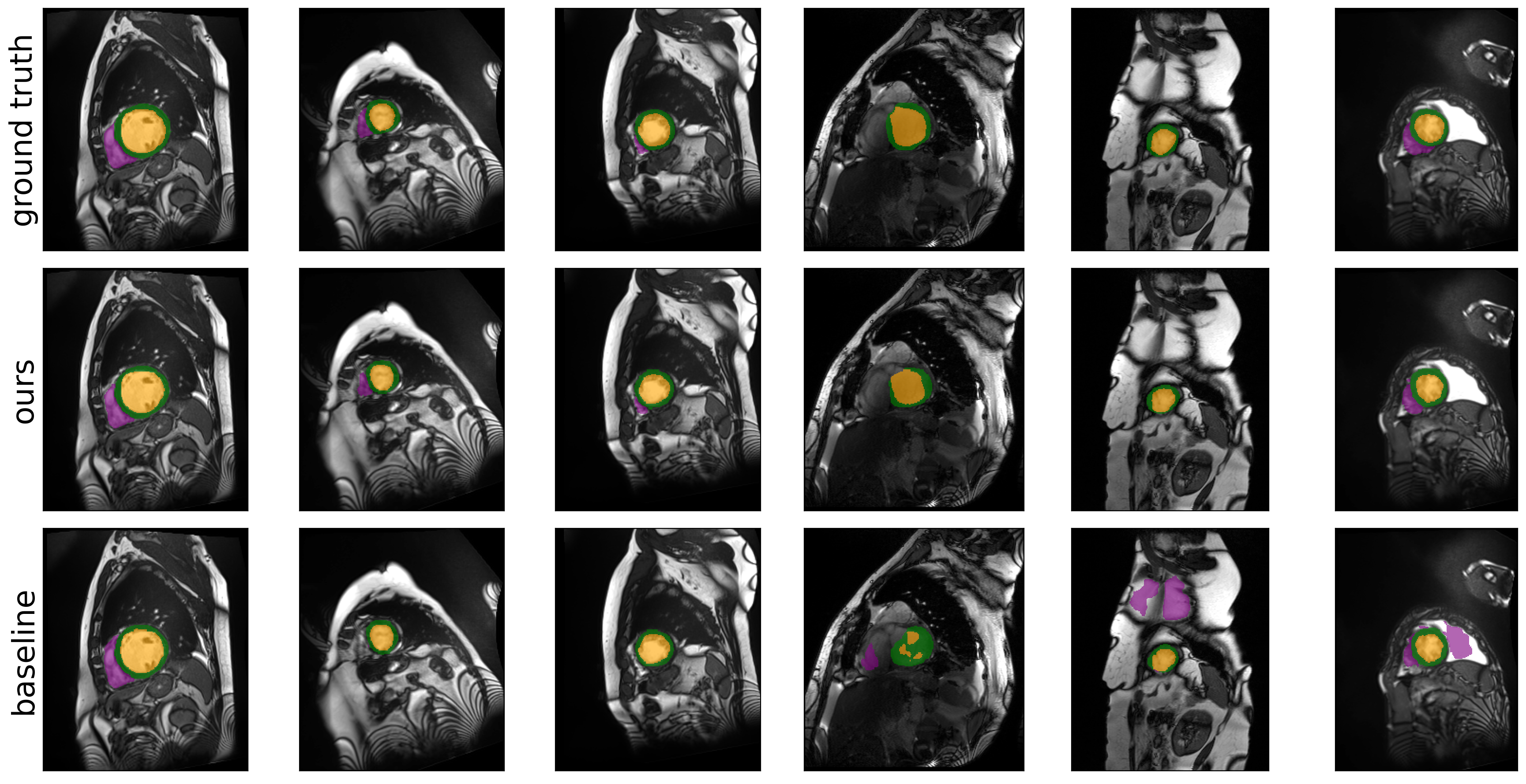
C.5.3 Visualization of Segmentation on Synapse with Distributional Shift
Figure C.2 visualizes the segmentation predictions on Synapse test slices made by models trained via AdaWAC (ours) and via the baseline (ERM+SGD) with TransUNet [26] on the half-sparse subset of the Synapse training set. We observe that, although the segmentation performances of both the baseline and AdaWAC are compromised by the extreme scarcity of label-dense samples and the severe distributional shift, AdaWAC provides more accurate predictions on the relative positions of organs, as well as less misclassification of organs (e.g., the baseline tends to misclassify other organs and the background as the left kidney). Nevertheless, due to the scarcity of labels, both the model trained with AdaWAC and that trained with the baseline fail to make good predictions on the segmentation boundaries.
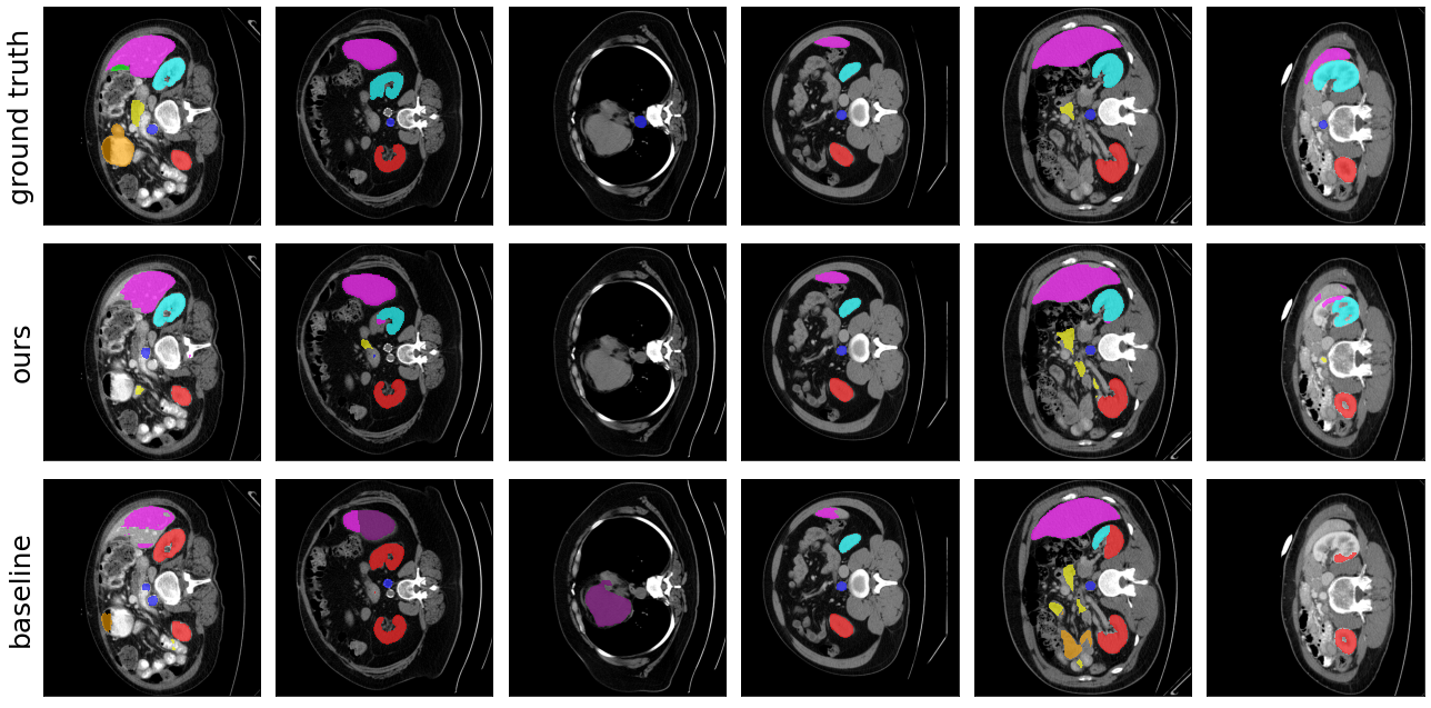
C.5.4 Experimental Results on Previous Metrics
In this section, we include the results of experiments on Synapse444Note that the numbers of correct metrics and metrics in TransUNet [26] on ACDC dataset are the same. dataset with metrics defined in TransUNet [26] for reference. In TransUNet [26], DSC is 1 when the sum of ground truth labels is zero (i.e., gt.sum() == 0) while the sum of predicted labels is nonzero (i.e., pred.sum() 0). However, according to the definition of dice scores, , the DSC for the above case should be 0 since the intersection is 0 and the denominator is non-zero. In our evaluation, we change the special condition for DSC as 1 to pred.sum == 0 and gt.sum() == 0 instead, in which case the denominator is 0.
Training Method DSC HD95 Aorta Gallbladder Kidney (L) Kidney (R) Liver Pancreas Spleen Stomach full baseline 77.32 29.23 87.46 63.54 82.06 77.76 94.10 54.06 85.07 74.54 AdaWAC 80.16 25.79 87.23 63.27 84.58 81.69 94.62 58.29 90.63 81.01 half-slice baseline 76.24 24.66 86.26 57.61 79.32 76.55 94.34 54.04 86.20 75.57 AdaWAC 78.14 29.75 86.66 62.28 81.36 78.84 94.60 57.95 85.38 78.01 half-vol baseline 72.65 35.86 83.29 43.70 78.25 77.25 92.92 51.32 83.80 70.66 AdaWAC 75.93 34.95 84.45 60.40 79.59 76.06 93.19 54.46 84.91 74.37 half-sparse baseline 0.00 0.00 0.00 0.00 0.00 0.00 0.00 0.00 0.00 0.00 AdaWAC 39.68 80.93 76.59 0.00 66.53 62.11 49.69 31.09 12.30 19.11
Method DSC HD95 Aorta Gallbladder Kidney (L) Kidney (R) Liver Pancreas Spleen Stomach baseline 77.32 29.23 87.46 63.54 82.06 77.76 94.10 54.06 85.07 74.54 trim-train 77.05 26.94 86.70 60.65 80.02 76.64 94.25 54.20 86.44 77.49 trim-ratio 75.30 28.59 87.35 57.29 78.70 72.22 94.18 52.32 86.31 74.03 trim-train+ACR 76.70 35.06 87.11 62.22 74.19 75.25 92.19 57.16 88.21 77.30 trim-ratio+ACR 79.02 33.59 86.82 61.67 83.52 81.22 94.07 59.06 88.08 77.71 AdaWAC (ours) 80.16 25.79 87.23 63.27 84.58 81.69 94.62 58.29 90.63 81.01
Method DSC HD95 Aorta Gallbladder Kidney (L) Kidney (R) Liver Pancreas Spleen Stomach baseline 77.32 29.23 87.46 63.54 82.06 77.76 94.10 54.06 85.07 74.54 reweight-only 77.72 29.24 86.15 62.31 82.96 80.28 93.42 55.86 85.29 75.49 ACR-only 78.93 31.65 87.96 62.67 81.79 80.21 94.52 60.41 88.07 75.83 AdaWAC-0.01 78.98 27.81 87.58 61.09 82.29 80.22 94.90 55.92 91.63 78.23 AdaWAC-1.0 80.16 25.79 87.23 63.27 84.58 81.69 94.62 58.29 90.63 81.01
References
- [1] Yariv Aizenbud, Gil Shabat, and Amir Averbuch. Randomized lu decomposition using sparse projections. Computers & Mathematics with Applications, 72(9):2525–2534, 2016.
- [2] Guillaume Alain, Alex Lamb, Chinnadhurai Sankar, Aaron Courville, and Yoshua Bengio. Variance reduction in sgd by distributed importance sampling. arXiv preprint arXiv:1511.06481, 2015.
- [3] David Anderson, Simon Du, Michael Mahoney, Christopher Melgaard, Kunming Wu, and Ming Gu. Spectral Gap Error Bounds for Improving CUR Matrix Decomposition and the Nyström Method. In Guy Lebanon and S. V. N. Vishwanathan, editors, Proceedings of the Eighteenth International Conference on Artificial Intelligence and Statistics, volume 38 of Proceedings of Machine Learning Research, pages 19–27, San Diego, California, USA, 09–12 May 2015. PMLR.
- [4] David Anderson and Ming Gu. An efficient, sparsity-preserving, online algorithm for low-rank approximation. In International Conference on Machine Learning, pages 156–165. PMLR, 2017.
- [5] Philip Bachman, Ouais Alsharif, and Doina Precup. Learning with pseudo-ensembles. Advances in neural information processing systems, 27:3365–3373, 2014.
- [6] Peter L. Bartlett and Shahar Mendelson. Rademacher and gaussian complexities: Risk bounds and structural results. J. Mach. Learn. Res., 3(null):463–482, March 2003.
- [7] Hritam Basak, Rajarshi Bhattacharya, Rukhshanda Hussain, and Agniv Chatterjee. An embarrassingly simple consistency regularization method for semi-supervised medical image segmentation. arXiv preprint arXiv:2202.00677, 2022.
- [8] Joshua D. Batson, Daniel A. Spielman, and Nikhil Srivastava. Twice-ramanujan sparsifiers. In Proceedings of the Forty-First Annual ACM Symposium on Theory of Computing, STOC ’09, pages 255–262, New York, NY, USA, 2009. Association for Computing Machinery.
- [9] Mario Bebendorf. Approximation of boundary element matrices. Numerische Mathematik, 86:565–589, 2000.
- [10] Aharon Ben-Tal, Dick den Hertog, Anja De Waegenaere, Bertrand Melenberg, and Gijs Rennen. Robust solutions of optimization problems affected by uncertain probabilities. Management Science, 59(2):341–357, 2013.
- [11] Gregory Benton, Marc Finzi, Pavel Izmailov, and Andrew Gordon Wilson. Learning invariances in neural networks. arXiv preprint arXiv:2010.11882, 2020.
- [12] David Berthelot, Nicholas Carlini, Ian Goodfellow, Nicolas Papernot, Avital Oliver, and Colin A Raffel. Mixmatch: A holistic approach to semi-supervised learning. Advances in neural information processing systems, 32, 2019.
- [13] David Berthelot, Rebecca Roelofs, Kihyuk Sohn, Nicholas Carlini, and Alex Kurakin. Adamatch: A unified approach to semi-supervised learning and domain adaptation. arXiv preprint arXiv:2106.04732, 2021.
- [14] Dimitri Bertsekas. Convex optimization theory, volume 1. Athena Scientific, 2009.
- [15] Jacob Bien, Ya Xu, and Michael Mahoney. Cur from a sparse optimization viewpoint. Annual Advances in Neural Information Processing Systems 24: Proceedings of the 2010 Conference, 11 2010.
- [16] Alberto Bietti, Luca Venturi, and Joan Bruna. On the sample complexity of learning with geometric stability. arXiv preprint arXiv:2106.07148, 2021.
- [17] Gerda Bortsova, Florian Dubost, Laurens Hogeweg, Ioannis Katramados, and Marleen de Bruijne. Semi-supervised medical image segmentation via learning consistency under transformations. In International Conference on Medical Image Computing and Computer-Assisted Intervention, pages 810–818. Springer, 2019.
- [18] Christos Boutsidis, Petros Drineas, and Malik Magdon-Ismail. Near-optimal column-based matrix reconstruction. SIAM Journal on Computing, 43(2):687–717, 2014.
- [19] Christos Boutsidis and Alex Gittens. Improved matrix algorithms via the subsampled randomized hadamard transform. SIAM Journal on Matrix Analysis and Applications, 34(3):1301–1340, 2013.
- [20] Christos Boutsidis, Prabhanjan Kambadur, and Alex Gittens. Spectral clustering via the power method-provably. In International conference on machine learning, pages 40–48. PMLR, 2015.
- [21] Christos Boutsidis and David P. Woodruff. Optimal cur matrix decompositions. In Proceedings of the Forty-Sixth Annual ACM Symposium on Theory of Computing, STOC ’14, pages 353–362, New York, NY, USA, 2014. Association for Computing Machinery.
- [22] Tianle Cai, Ruiqi Gao, Jason D. Lee, and Qi Lei. A theory of label propagation for subpopulation shift, 2021.
- [23] Hu Cao, Yueyue Wang, Joy Chen, Dongsheng Jiang, Xiaopeng Zhang, Qi Tian, and Manning Wang. Swin-unet: Unet-like pure transformer for medical image segmentation. arXiv preprint arXiv:2105.05537, 2021.
- [24] Tony F. Chan. Rank revealing qr factorizations. Linear Algebra and its Applications, 88-89:67–82, 1987.
- [25] Cheng Chen, Ming Gu, Zhihua Zhang, Weinan Zhang, and Yong Yu. Efficient spectrum-revealing cur matrix decomposition. In International Conference on Artificial Intelligence and Statistics, pages 766–775. PMLR, 2020.
- [26] Jieneng Chen, Yongyi Lu, Qihang Yu, Xiangde Luo, Ehsan Adeli, Yan Wang, Le Lu, Alan L Yuille, and Yuyin Zhou. Transunet: Transformers make strong encoders for medical image segmentation. arXiv preprint arXiv:2102.04306, 2021.
- [27] Shuxiao Chen, Edgar Dobriban, and Jane H Lee. A group-theoretic framework for data augmentation. Journal of Machine Learning Research, 21(245):1–71, 2020.
- [28] Ting Chen, Simon Kornblith, Mohammad Norouzi, and Geoffrey Hinton. A simple framework for contrastive learning of visual representations. In International conference on machine learning, pages 1597–1607. PMLR, 2020.
- [29] Ali Civril and Malik Magdon-Ismail. Exponential inapproximability of selecting a maximum volume sub-matrix. Algorithmica, 65(1):159–176, 2013.
- [30] Kenneth L. Clarkson and David P. Woodruff. Low-rank approximation and regression in input sparsity time. J. ACM, 63(6), January 2017.
- [31] Michael B. Cohen, Yin Tat Lee, Cameron Musco, Christopher Musco, Richard Peng, and Aaron Sidford. Uniform sampling for matrix approximation. In Proceedings of the 2015 Conference on Innovations in Theoretical Computer Science, ITCS ’15, pages 181–190, New York, NY, USA, 2015. Association for Computing Machinery.
- [32] Taco Cohen and Max Welling. Group equivariant convolutional networks. In International conference on machine learning, pages 2990–2999. PMLR, 2016.
- [33] Alice Cortinovis and Daniel Kressner. Low-rank approximation in the frobenius norm by column and row subset selection. SIAM Journal on Matrix Analysis and Applications, 41(4):1651–1673, 2020.
- [34] Ekin D Cubuk, Barret Zoph, Dandelion Mane, Vijay Vasudevan, and Quoc V Le. Autoaugment: Learning augmentation strategies from data. In Proceedings of the IEEE/CVF Conference on Computer Vision and Pattern Recognition, pages 113–123, 2019.
- [35] Ekin D Cubuk, Barret Zoph, Jonathon Shlens, and Quoc V Le. Randaugment: Practical automated data augmentation with a reduced search space. In Proceedings of the IEEE/CVF Conference on Computer Vision and Pattern Recognition Workshops, pages 702–703, 2020.
- [36] Tri Dao, Albert Gu, Alexander Ratner, Virginia Smith, Chris De Sa, and Christopher Ré. A kernel theory of modern data augmentation. In International Conference on Machine Learning, pages 1528–1537. PMLR, 2019.
- [37] Kenneth R Davidson and Stanislaw J Szarek. Local operator theory, random matrices and banach spaces. Handbook of the geometry of Banach spaces, 1(317-366):131, 2001.
- [38] C. Davis and W. M. Kahan. The rotation of eigenvectors by a perturbation. III. sinum, 7(1):1–46, 1970.
- [39] Michal Derezinski, Rajiv Khanna, and Michael W. Mahoney. Improved guarantees and a multiple-descent curve for the column subset selection problem and the nyström method. CoRR, abs/2002.09073, 2020.
- [40] Michał Dereziński and Michael Mahoney. Determinantal point processes in randomized numerical linear algebra. Notices of the American Mathematical Society, 68:1, 01 2021.
- [41] Amit Deshpande and Luis Rademacher. Efficient volume sampling for row/column subset selection. In 2010 IEEE 51st Annual Symposium on Foundations of Computer Science, pages 329–338, 2010.
- [42] Amit Deshpande, Luis Rademacher, Santosh Vempala, and Grant Wang. Matrix approximation and projective clustering via volume sampling. Theory of Computing, 2(12):225–247, 2006.
- [43] Terrance DeVries and Graham W Taylor. Improved regularization of convolutional neural networks with cutout. arXiv preprint arXiv:1708.04552, 2017.
- [44] Yijun Dong, Chao Chen, Per-Gunnar Martinsson, and Katherine Pearce. Robust blockwise random pivoting: Fast and accurate adaptive interpolative decomposition. arXiv preprint arXiv:2309.16002, 2023.
- [45] Yijun Dong and Per-Gunnar Martinsson. Simpler is better: a comparative study of randomized pivoting algorithms for cur and interpolative decompositions. Advances in Computational Mathematics, 49(4):66, 2023.
- [46] Yijun Dong, Per-Gunnar Martinsson, and Yuji Nakatsukasa. Efficient bounds and estimates for canonical angles in randomized subspace approximations. arXiv preprint arXiv:2211.04676, 2022.
- [47] Yijun Dong, Kevin Miller, Qi Lei, and Rachel Ward. Cluster-aware semi-supervised learning: Relational knowledge distillation provably learns clustering. arXiv preprint arXiv:2307.11030, 2023.
- [48] Yijun Dong, Yuege Xie, and Rachel Ward. Adaptively weighted data augmentation consistency regularization for robust optimization under concept shift. In Proceedings of the 40th International Conference on Machine Learning, volume 202 of Proceedings of Machine Learning Research, pages 8296–8316. PMLR, 23–29 Jul 2023.
- [49] Petros Drineas, Malik Magdon-Ismail, Michael W Mahoney, and David P Woodruff. Fast approximation of matrix coherence and statistical leverage. The Journal of Machine Learning Research, 13(1):3475–3506, 2012.
- [50] Petros Drineas, Michael W Mahoney, and Shan Muthukrishnan. Relative-error cur matrix decompositions. SIAM Journal on Matrix Analysis and Applications, 30(2):844–881, 2008.
- [51] Zlatko Drmač and Serkan Gugercin. A new selection operator for the discrete empirical interpolation method—improved a priori error bound and extensions. SIAM Journal on Scientific Computing, 38(2):A631–A648, 2016.
- [52] Simon S. Du, Wei Hu, Sham M. Kakade, Jason D. Lee, and Qi Lei. Few-shot learning via learning the representation, provably, 2020.
- [53] John Duchi, Peter Glynn, and Hongseok Namkoong. Statistics of robust optimization: A generalized empirical likelihood approach. arXiv preprint arXiv:1610.03425, 2016.
- [54] John Duchi and Hongseok Namkoong. Learning models with uniform performance via distributionally robust optimization. arXiv preprint arXiv:1810.08750, 2018.
- [55] Carl Eckart and Gale Young. The approximation of one matrix by another of lower rank. Psychometrika, 1(3):211–218, Sep 1936.
- [56] Geoffrey French, Michal Mackiewicz, and Mark Fisher. Self-ensembling for visual domain adaptation. arXiv preprint arXiv:1706.05208, 2017.
- [57] Siddhant Garg and Yingyu Liang. Functional regularization for representation learning: A unified theoretical perspective. arXiv preprint arXiv:2008.02447, 2020.
- [58] George A. Geist and Charles H. Romine. $lu$ factorization algorithms on distributed-memory multiprocessor architectures. SIAM Journal on Scientific and Statistical Computing, 9(4):639–649, 1988.
- [59] Gene H Golub and Charles F Van Loan. Matrix computations. JHU press, Baltimore, MD, USA, 2013.
- [60] Siddharth Gopal. Adaptive sampling for sgd by exploiting side information. In Proceedings of the 33rd International Conference on International Conference on Machine Learning - Volume 48, ICML’16, pages 364–372. JMLR.org, 2016.
- [61] S.A. Goreinov, E.E. Tyrtyshnikov, and N.L. Zamarashkin. A theory of pseudoskeleton approximations. Linear Algebra and its Applications, 261(1):1–21, 1997.
- [62] Laura Grigori, James W. Demmel, and Hua Xiang. Calu: A communication optimal lu factorization algorithm. SIAM Journal on Matrix Analysis and Applications, 32(4):1317–1350, 2011.
- [63] Jean-Bastien Grill, Florian Strub, Florent Altché, Corentin Tallec, Pierre Richemond, Elena Buchatskaya, Carl Doersch, Bernardo Avila Pires, Zhaohan Guo, Mohammad Gheshlaghi Azar, et al. Bootstrap your own latent-a new approach to self-supervised learning. Advances in neural information processing systems, 33:21271–21284, 2020.
- [64] M. Gu. Subspace iteration randomization and singular value problems. SIAM Journal on Scientific Computing, 37(3):A1139–A1173, 2015.
- [65] Ming Gu and Stanley C. Eisenstat. Efficient algorithms for computing a strong rank-revealing qr factorization. SIAM Journal on Scientific Computing, 17(4):848–869, 1996.
- [66] Guy Hacohen and Daphna Weinshall. On the power of curriculum learning in training deep networks. In International Conference on Machine Learning, pages 2535–2544. PMLR, 2019.
- [67] Jamie Haddock, Deanna Needell, Elizaveta Rebrova, and William Swartworth. Quantile-based iterative methods for corrupted systems of linear equations. SIAM Journal on Matrix Analysis and Applications, 43(2):605–637, 2022.
- [68] N. Halko, P. G. Martinsson, and J. A. Tropp. Finding structure with randomness: Probabilistic algorithms for constructing approximate matrix decompositions. SIAM Review, 53(2):217–288, 2011.
- [69] Jeff Z HaoChen, Colin Wei, Adrien Gaidon, and Tengyu Ma. Provable guarantees for self-supervised deep learning with spectral contrastive loss. arXiv preprint arXiv:2106.04156, 2021.
- [70] Kaiming He, Haoqi Fan, Yuxin Wu, Saining Xie, and Ross Girshick. Momentum contrast for unsupervised visual representation learning. In Proceedings of the IEEE/CVF conference on computer vision and pattern recognition, pages 9729–9738, 2020.
- [71] Kaiming He, Xiangyu Zhang, Shaoqing Ren, and Jian Sun. Deep residual learning for image recognition. In Proceedings of the IEEE conference on computer vision and pattern recognition, pages 770–778, 2016.
- [72] Zhuoxun He, Lingxi Xie, Xin Chen, Ya Zhang, Yanfeng Wang, and Qi Tian. Data augmentation revisited: Rethinking the distribution gap between clean and augmented data. arXiv preprint arXiv:1909.09148, 2019.
- [73] Ken Ho, Sheehan Olver, Tony Kelman, Elias Jarlebring, Julia TagBot, and Mikael Slevinsky. Lowrankapprox,jl: v0.4.3. https://github.com/JuliaMatrices/LowRankApprox.jl, 2020.
- [74] Y. P. Hong and C.-T. Pan. Rank-revealing qr factorizations and the singular value decomposition. Mathematics of Computation, 58(197):213–232, 1992.
- [75] Roger A. Horn and Charles R. Johnson. Matrix Analysis. Cambridge University Press, 2 edition, 2012.
- [76] Alston S. Householder. Unitary triangularization of a nonsymmetric matrix. J. ACM, 5(4):339–342, October 1958.
- [77] Pavel Iakubovskii. Segmentation models pytorch. https://github.com/qubvel/segmentation_models.pytorch, 2019.
- [78] Piotr Indyk and Rajeev Motwani. Approximate nearest neighbors: Towards removing the curse of dimensionality. In Proceedings of the Thirtieth Annual ACM Symposium on Theory of Computing, STOC ’98, page 604–613, New York, NY, USA, 1998. Association for Computing Machinery.
- [79] W. Kahan. Numerical linear algebra. Canadian Mathematical Bulletin, 9(5):757–801, 1966.
- [80] Davood Karimi, Haoran Dou, Simon K Warfield, and Ali Gholipour. Deep learning with noisy labels: Exploring techniques and remedies in medical image analysis. Medical Image Analysis, 65:101759, 2020.
- [81] Angelos Katharopoulos and François Fleuret. Not all samples are created equal: Deep learning with importance sampling. In International conference on machine learning, pages 2525–2534. PMLR, 2018.
- [82] Kenji Kawaguchi and Haihao Lu. Ordered sgd: A new stochastic optimization framework for empirical risk minimization. In International Conference on Artificial Intelligence and Statistics, pages 669–679. PMLR, 2020.
- [83] Kezhong Zhao, M. N. Vouvakis, and Jin-Fa Lee. The adaptive cross approximation algorithm for accelerated method of moments computations of emc problems. IEEE Transactions on Electromagnetic Compatibility, 47(4):763–773, 2005.
- [84] Alex Krizhevsky, Ilya Sutskever, and Geoffrey E Hinton. Imagenet classification with deep convolutional neural networks. Advances in neural information processing systems, 25:1097–1105, 2012.
- [85] Michael Kuchnik and Virginia Smith. Efficient augmentation via data subsampling. arXiv preprint arXiv:1810.05222, 2018.
- [86] J. Kuczyński and H. Woźniakowski. Estimating the largest eigenvalue by the power and lanczos algorithms with a random start. SIAM Journal on Matrix Analysis and Applications, 13(4):1094–1122, 1992.
- [87] J. Kurzak, P. Luszczek, M. Faverge, and J. Dongarra. Lu factorization with partial pivoting for a multicore system with accelerators. IEEE Transactions on Parallel and Distributed Systems, 24(8):1613–1621, 2013.
- [88] Samuli Laine and Timo Aila. Temporal ensembling for semi-supervised learning. arXiv preprint arXiv:1610.02242, 2016.
- [89] Michel Ledoux and Michel Talagrand. Probability in Banach Spaces: isoperimetry and processes. Springer Science & Business Media, 2013.
- [90] Xiaomeng Li, Lequan Yu, Hao Chen, Chi-Wing Fu, Lei Xing, and Pheng-Ann Heng. Transformation-consistent self-ensembling model for semisupervised medical image segmentation. IEEE Transactions on Neural Networks and Learning Systems, 32(2):523–534, 2020.
- [91] Zhiyuan Li, Ruosong Wang, Dingli Yu, Simon S Du, Wei Hu, Ruslan Salakhutdinov, and Sanjeev Arora. Enhanced convolutional neural tangent kernels. arXiv preprint arXiv:1911.00809, 2019.
- [92] Edo Liberty, Franco Woolfe, Per-Gunnar Martinsson, Vladimir Rokhlin, and Mark Tygert. Randomized algorithms for the low-rank approximation of matrices. Proceedings of the National Academy of Sciences, 104(51):20167–20172, 2007.
- [93] Sungbin Lim, Ildoo Kim, Taesup Kim, Chiheon Kim, and Sungwoong Kim. Fast autoaugment. Advances in Neural Information Processing Systems, 32:6665–6675, 2019.
- [94] Ilya Loshchilov and Frank Hutter. Online batch selection for faster training of neural networks. arXiv preprint arXiv:1511.06343, 2015.
- [95] Clare Lyle, Marta Kwiatkowksa, and Yarin Gal. An analysis of the effect of invariance on generalization in neural networks. In International conference on machine learning Workshop on Understanding and Improving Generalization in Deep Learning, 2019.
- [96] Michael W Mahoney and Petros Drineas. Cur matrix decompositions for improved data analysis. Proceedings of the National Academy of Sciences, 106(3):697–702, 2009.
- [97] Diego Marcos, Michele Volpi, Nikos Komodakis, and Devis Tuia. Rotation equivariant vector field networks. In Proceedings of the IEEE International Conference on Computer Vision, pages 5048–5057, 2017.
- [98] Per-Gunnar Martinsson. Randomized methods for matrix computations. The Mathematics of Data, 25(4):187–231, 2019.
- [99] Per-Gunnar Martinsson, Vladimir Rokhlin, and Mark Tygert. A randomized algorithm for the decomposition of matrices. Applied and Computational Harmonic Analysis, 30(1):47–68, 2011.
- [100] Per-Gunnar Martinsson and Joel A. Tropp. Randomized numerical linear algebra: Foundations and algorithms. Acta Numerica, 29:403–572, 2020.
- [101] Per-Gunnar Martinsson and Joel A. Tropp. Randomized numerical linear algebra: Foundations and algorithms. Acta Numerica, 29:403–572, 2020.
- [102] Song Mei, Theodor Misiakiewicz, and Andrea Montanari. Learning with invariances in random features and kernel models. arXiv preprint arXiv:2102.13219, 2021.
- [103] Xiangrui Meng and Michael W. Mahoney. Low-distortion subspace embeddings in input-sparsity time and applications to robust linear regression. In Proceedings of the Forty-Fifth Annual ACM Symposium on Theory of Computing, STOC ’13, pages 91–100, New York, NY, USA, 2013. Association for Computing Machinery.
- [104] C. Meszaros. Meszaros/large, lp sequence: large000 to large036. http://old.sztaki.hu/ meszaros/public_ftp/lptestset/, 2004.
- [105] Raphael A Meyer, Cameron Musco, Christopher Musco, and David P Woodruff. Hutch++: Optimal stochastic trace estimation. In Symposium on Simplicity in Algorithms (SOSA), pages 142–155. SIAM, 2021.
- [106] Fausto Milletari, Nassir Navab, and Seyed-Ahmad Ahmadi. V-net: Fully convolutional neural networks for volumetric medical image segmentation. In 2016 Fourth International Conference on 3D Vision (3DV), pages 565–571, 2016.
- [107] L Miranian and Ming Gu. Strong rank revealing lu factorizations. Linear Algebra and its Applications, 367:1–16, 07 2003.
- [108] Cameron Musco and Christopher Musco. Randomized block krylov methods for stronger and faster approximate singular value decomposition. In Proceedings of the 28th International Conference on Neural Information Processing Systems - Volume 1, NIPS’15, pages 1396–1404, Cambridge, MA, USA, 2015. MIT Press.
- [109] Yuji Nakatsukasa. Sharp error bounds for ritz vectors and approximate singular vectors. Math. Comput., 89:1843–1866, 2020.
- [110] Deanna Needell, Rachel Ward, and Nati Srebro. Stochastic gradient descent, weighted sampling, and the randomized kaczmarz algorithm. Advances in neural information processing systems, 27, 2014.
- [111] J. Nelson and H. L. Nguyên. Osnap: Faster numerical linear algebra algorithms via sparser subspace embeddings. In 2013 IEEE 54th Annual Symposium on Foundations of Computer Science, pages 117–126, 2013.
- [112] A. Nemirovski, A. Juditsky, G. Lan, and A. Shapiro. Robust stochastic approximation approach to stochastic programming. SIAM Journal on Optimization, 19(4):1574–1609, 2009.
- [113] C.-T. Pan. On the existence and computation of rank-revealing lu factorizations. Linear Algebra and its Applications, 316(1):199–222, 2000. Special Issue: Conference celebrating the 60th birthday of Robert J. Plemmons.
- [114] Victor Y. Pan, Guoliang Qian, and Xiaodong Yan. Random multipliers numerically stabilize gaussian and block gaussian elimination: Proofs and an extension to low-rank approximation. Linear Algebra and its Applications, 481:202–234, 2015.
- [115] Victor Y. Pan and Liang Zhao. Numerically safe gaussian elimination with no pivoting. Linear Algebra and its Applications, 527:349–383, 2017.
- [116] G. Peters and J. H. Wilkinson. On the stability of gauss-jordan elimination with pivoting. Commun. ACM, 18(1):20–24, January 1975.
- [117] Shashank Rajput, Zhili Feng, Zachary Charles, Po-Ling Loh, and Dimitris Papailiopoulos. Does data augmentation lead to positive margin? In International Conference on Machine Learning, pages 5321–5330. PMLR, 2019.
- [118] Vladimir Rokhlin and Mark Tygert. A fast randomized algorithm for overdetermined linear least-squares regression. Proceedings of the National Academy of Sciences, 105(36):13212–13217, 2008.
- [119] Olaf Ronneberger, Philipp Fischer, and Thomas Brox. U-net: Convolutional networks for biomedical image segmentation. In International Conference on Medical image computing and computer-assisted intervention, pages 234–241. Springer, 2015.
- [120] Mark Rudelson. Invertibility of random matrices: Norm of the inverse. Annals of Mathematics, 168(2):575–600, 2008.
- [121] Stuart J Russell and Peter Norvig. Artificial intelligence: a modern approach. malaysia, 2016.
- [122] Shiori Sagawa, Pang Wei Koh, Tatsunori B Hashimoto, and Percy Liang. Distributionally robust neural networks for group shifts: On the importance of regularization for worst-case generalization. arXiv preprint arXiv:1911.08731, 2019.
- [123] Arvind K Saibaba. Randomized subspace iteration: Analysis of canonical angles and unitarily invariant norms. SIAM Journal on Matrix Analysis and Applications, 40(1):23–48, 2019.
- [124] Mehdi Sajjadi, Mehran Javanmardi, and Tolga Tasdizen. Regularization with stochastic transformations and perturbations for deep semi-supervised learning. Advances in neural information processing systems, 29:1163–1171, 2016.
- [125] Rico Sennrich, Barry Haddow, and Alexandra Birch. Improving neural machine translation models with monolingual data. arXiv preprint arXiv:1511.06709, 2015.
- [126] Gil Shabat, Yaniv Shmueli, Yariv Aizenbud, and Amir Averbuch. Randomized lu decomposition. Applied and Computational Harmonic Analysis, 44(2):246–272, 2018.
- [127] Vatsal Shah, Xiaoxia Wu, and Sujay Sanghavi. Choosing the sample with lowest loss makes sgd robust. In Proceedings of the Twenty Third International Conference on Artificial Intelligence and Statistics, volume 108 of Proceedings of Machine Learning Research, pages 2120–2130, Online, 26–28 Aug 2020. PMLR.
- [128] Han Shao, Omar Montasser, and Avrim Blum. A theory of pac learnability under transformation invariances. arXiv preprint arXiv:2202.07552, 2022.
- [129] Ruoqi Shen, Sebastien Bubeck, and Suriya Gunasekar. Data augmentation as feature manipulation. In International Conference on Machine Learning, pages 19773–19808. PMLR, 2022.
- [130] Yanyao Shen and Sujay Sanghavi. Learning with bad training data via iterative trimmed loss minimization. In International Conference on Machine Learning, pages 5739–5748. PMLR, 2019.
- [131] Connor Shorten and Taghi M Khoshgoftaar. A survey on image data augmentation for deep learning. Journal of Big Data, 6(1):1–48, 2019.
- [132] Patrice Y Simard, Yann A LeCun, John S Denker, and Bernard Victorri. Transformation invariance in pattern recognition—tangent distance and tangent propagation. In Neural networks: tricks of the trade, pages 239–274. Springer, 1998.
- [133] Karen Simonyan and Andrew Zisserman. Very deep convolutional networks for large-scale image recognition. arXiv preprint arXiv:1409.1556, 2014.
- [134] Maurice Sion. On general minimax theorems. Pacific Journal of Mathematics, 8(1):171 – 176, 1958.
- [135] Kihyuk Sohn, David Berthelot, Chun-Liang Li, Zizhao Zhang, Nicholas Carlini, Ekin D Cubuk, Alex Kurakin, Han Zhang, and Colin Raffel. Fixmatch: Simplifying semi-supervised learning with consistency and confidence. arXiv preprint arXiv:2001.07685, 2020.
- [136] Edgar Solomonik and James Demmel. Communication-optimal parallel 2.5d matrix multiplication and lu factorization algorithms. In Emmanuel Jeannot, Raymond Namyst, and Jean Roman, editors, Euro-Par 2011 Parallel Processing, pages 90–109, Berlin, Heidelberg, 2011. Springer Berlin Heidelberg.
- [137] D. C. Sorensen and Mark Embree. A deim induced cur factorization. SIAM Journal on Scientific Computing, 38(3):A1454–A1482, 2016.
- [138] Danny C Sorensen and Mark Embree. A deim induced cur factorization. SIAM Journal on Scientific Computing, 38(3):A1454–A1482, 2016.
- [139] Ivan Sosnovik, Michał Szmaja, and Arnold Smeulders. Scale-equivariant steerable networks. arXiv preprint arXiv:1910.11093, 2019.
- [140] Saeid Asgari Taghanaki, Kumar Abhishek, Joseph Paul Cohen, Julien Cohen-Adad, and Ghassan Hamarneh. Deep semantic segmentation of natural and medical images: A review, 2019.
- [141] Saeid Asgari Taghanaki, Yefeng Zheng, S Kevin Zhou, Bogdan Georgescu, Puneet Sharma, Daguang Xu, Dorin Comaniciu, and Ghassan Hamarneh. Combo loss: Handling input and output imbalance in multi-organ segmentation. Computerized Medical Imaging and Graphics, 75:24–33, 2019.
- [142] Yuxing Tang, Xiaosong Wang, Adam P Harrison, Le Lu, Jing Xiao, and Ronald M Summers. Attention-guided curriculum learning for weakly supervised classification and localization of thoracic diseases on chest radiographs. In International Workshop on Machine Learning in Medical Imaging, pages 249–258. Springer, 2018.
- [143] Christopher Tensmeyer and Tony Martinez. Improving invariance and equivariance properties of convolutional neural networks, 2017.
- [144] Lloyd N Trefethen and David Bau. Numerical linear algebra, volume 181. Siam, Philadelphia, PA, USA, 2022.
- [145] Lloyd N. Trefethen and Robert S. Schreiber. Average-case stability of gaussian elimination. SIAM Journal on Matrix Analysis and Applications, 11(3):335–360, 1990.
- [146] Joel A. Tropp. Improved analysis of the subsampled randomized hadamard transform. Advances in Adaptive Data Analysis, 03(01n02):115–126, 2011.
- [147] Joel A Tropp, Alp Yurtsever, Madeleine Udell, and Volkan Cevher. Fixed-rank approximation of a positive-semidefinite matrix from streaming data. Advances in Neural Information Processing Systems, 30, 2017.
- [148] Joel A. Tropp, Alp Yurtsever, Madeleine Udell, and Volkan Cevher. Streaming low-rank matrix approximation with an application to scientific simulation. SIAM Journal on Scientific Computing, 41(4):A2430–A2463, 2019.
- [149] Jonathan G Tullis and Aaron S Benjamin. On the effectiveness of self-paced learning. Journal of memory and language, 64(2):109–118, 2011.
- [150] E. Tyrtyshnikov. Incomplete cross approximation in the mosaic-skeleton method. Computing, 64(4):367–380, Jun 2000.
- [151] Roman Vershynin. High-dimensional probability: An introduction with applications in data science, volume 47. Cambridge university press, 2018.
- [152] Julius von Kügelgen, Yash Sharma, Luigi Gresele, Wieland Brendel, Bernhard Schölkopf, Michel Besserve, and Francesco Locatello. Self-supervised learning with data augmentations provably isolates content from style. arXiv preprint arXiv:2106.04619, 2021.
- [153] Sergey Voronin and Per-Gunnar Martinsson. Efficient algorithms for cur and interpolative matrix decompositions. Advances in Computational Mathematics, 43(3):495–516, Jun 2017.
- [154] Martin J Wainwright. High-dimensional statistics: A non-asymptotic viewpoint, volume 48. Cambridge University Press, 2019.
- [155] Martin J. Wainwright. High-Dimensional Statistics: A Non-Asymptotic Viewpoint. Cambridge Series in Statistical and Probabilistic Mathematics. Cambridge University Press, 2019.
- [156] Haohan Wang, Zeyi Huang, Xindi Wu, and Eric P Xing. Squared norm as consistency loss for leveraging augmented data to learn robust and invariant representations. arXiv preprint arXiv:2011.13052, 2020.
- [157] Shusen Wang and Zhihua Zhang. A scalable cur matrix decomposition algorithm: Lower time complexity and tighter bound. In Proceedings of the 25th International Conference on Neural Information Processing Systems - Volume 1, NIPS’12, pages 647–655, Red Hook, NY, USA, 2012. Curran Associates Inc.
- [158] Xi Wang, Hao Chen, Huiling Xiang, Huangjing Lin, Xi Lin, and Pheng-Ann Heng. Deep virtual adversarial self-training with consistency regularization for semi-supervised medical image classification. Medical image analysis, 70:102010, 2021.
- [159] Xin Wang, Yudong Chen, and Wenwu Zhu. A survey on curriculum learning. IEEE Transactions on Pattern Analysis and Machine Intelligence, 2021.
- [160] Yisen Wang, Weiyang Liu, Xingjun Ma, James Bailey, Hongyuan Zha, Le Song, and Shu-Tao Xia. Iterative learning with open-set noisy labels. In Proceedings of the IEEE conference on computer vision and pattern recognition, pages 8688–8696, 2018.
- [161] Per-Åke Wedin. Perturbation theory for pseudo-inverses. bit, 13(2):217–232, 1973.
- [162] Colin Wei, Kendrick Shen, Yining Chen, and Tengyu Ma. Theoretical analysis of self-training with deep networks on unlabeled data, 2021.
- [163] Zixin Wen and Yuanzhi Li. Toward understanding the feature learning process of self-supervised contrastive learning. arXiv preprint arXiv:2105.15134, 2021.
- [164] Ken C. L. Wong, Mehdi Moradi, Hui Tang, and Tanveer Syeda-Mahmood. 3d segmentation with exponential logarithmic loss for highly unbalanced object sizes. In Alejandro F. Frangi, Julia A. Schnabel, Christos Davatzikos, Carlos Alberola-López, and Gabor Fichtinger, editors, Medical Image Computing and Computer Assisted Intervention – MICCAI 2018, pages 612–619, Cham, 2018. Springer International Publishing.
- [165] David P. Woodruff. Sketching as a tool for numerical linear algebra. Found. Trends Theor. Comput. Sci., 10(1–2):1–157, October 2014.
- [166] Franco Woolfe, Edo Liberty, Vladimir Rokhlin, and Mark Tygert. A fast randomized algorithm for the approximation of matrices. Applied and Computational Harmonic Analysis, 25(3):335–366, 2008.
- [167] Daniel E Worrall, Stephan J Garbin, Daniyar Turmukhambetov, and Gabriel J Brostow. Harmonic networks: Deep translation and rotation equivariance. In Proceedings of the IEEE Conference on Computer Vision and Pattern Recognition, pages 5028–5037, 2017.
- [168] Daniel E Worrall and Max Welling. Deep scale-spaces: Equivariance over scale. arXiv preprint arXiv:1905.11697, 2019.
- [169] Sen Wu, Hongyang Zhang, Gregory Valiant, and Christopher Ré. On the generalization effects of linear transformations in data augmentation. In International Conference on Machine Learning, pages 10410–10420. PMLR, 2020.
- [170] Xiaoxia Wu, Yuege Xie, Simon Shaolei Du, and Rachel Ward. Adaloss: A computationally-efficient and provably convergent adaptive gradient method. Proceedings of the AAAI Conference on Artificial Intelligence, 36(8):8691–8699, Jun. 2022.
- [171] Zhirong Wu, Yuanjun Xiong, Stella X Yu, and Dahua Lin. Unsupervised feature learning via non-parametric instance discrimination. In Proceedings of the IEEE conference on computer vision and pattern recognition, pages 3733–3742, 2018.
- [172] Qizhe Xie, Minh-Thang Luong, Eduard Hovy, and Quoc V Le. Self-training with noisy student improves imagenet classification. In Proceedings of the IEEE/CVF Conference on Computer Vision and Pattern Recognition, pages 10687–10698, 2020.
- [173] Shuo Yang, Yijun Dong, Rachel Ward, Inderjit S Dhillon, Sujay Sanghavi, and Qi Lei. Sample efficiency of data augmentation consistency regularization. In International Conference on Artificial Intelligence and Statistics, pages 3825–3853. PMLR, 2023.
- [174] Michael Yeung, Evis Sala, Carola-Bibiane Schönlieb, and Leonardo Rundo. Unified focal loss: Generalising dice and cross entropy-based losses to handle class imbalanced medical image segmentation. Computerized Medical Imaging and Graphics, 95:102026, 2022.
- [175] Sangdoo Yun, Dongyoon Han, Seong Joon Oh, Sanghyuk Chun, Junsuk Choe, and Youngjoon Yoo. Cutmix: Regularization strategy to train strong classifiers with localizable features. In Proceedings of the IEEE/CVF International Conference on Computer Vision, pages 6023–6032, 2019.
- [176] Sergey Zagoruyko and Nikos Komodakis. Wide residual networks. arXiv preprint arXiv:1605.07146, 2016.
- [177] Hongyi Zhang, Moustapha Cisse, Yann N Dauphin, and David Lopez-Paz. mixup: Beyond empirical risk minimization. arXiv preprint arXiv:1710.09412, 2017.
- [178] Yi Zhang, Bin Zhou, Lei Chen, Yulin Wu, and Hongchao Zhou. Multi-transformation consistency regularization for semi-supervised medical image segmentation. In 2021 4th International Conference on Artificial Intelligence and Big Data (ICAIBD), pages 485–489. IEEE, 2021.
- [179] Amy Zhao, Guha Balakrishnan, Fredo Durand, John V Guttag, and Adrian V Dalca. Data augmentation using learned transformations for one-shot medical image segmentation. In Proceedings of the IEEE/CVF conference on computer vision and pattern recognition, pages 8543–8553, 2019.
- [180] Peilin Zhao and Tong Zhang. Stochastic optimization with importance sampling for regularized loss minimization. In international conference on machine learning, pages 1–9. PMLR, 2015.
- [181] Hong-Yu Zhou, Chengdi Wang, Haofeng Li, Gang Wang, Shu Zhang, Weimin Li, and Yizhou Yu. Ssmd: semi-supervised medical image detection with adaptive consistency and heterogeneous perturbation. Medical Image Analysis, 72:102117, 2021.
- [182] Yanzhao Zhou, Qixiang Ye, Qiang Qiu, and Jianbin Jiao. Oriented response networks. In Proceedings of the IEEE Conference on Computer Vision and Pattern Recognition, pages 519–528, 2017.
- [183] Åke Björck and Gene H. Golub. Numerical methods for computing angles between linear subspaces. Mathematics of Computation, 27(123):579–594, 1973.
- [184] Ali Çivril and Malik Magdon-Ismail. On selecting a maximum volume sub-matrix of a matrix and related problems. Theoretical Computer Science, 410(47):4801–4811, 2009.
Index
Vita
Yijun Dong was born in Shanghai, China in October 1995 and grew up there before college. She obtained a Bachelor of Science in Applied Mathematics and Engineering Science from Emory University in May 2018 where she got her first taste of research in biophysics and soft matter physics. In August 2018, she began her doctoral study in Computational Science, Engineering, and Mathematics at the Oden Institute of the University of Texas at Austin. Her primary research interests are randomized numerical linear algebra and statistical learning theory. In 2021 and 2022, she spent two summers at Dell Technologies working on edge computing and semi-supervised tabular learning. Upon completing her graduate study in May 2023, she expects to continue her postdoctoral research as a Courant Instructor at the Courant Institute of New York University.
Address: ydong@utexas.edu
This dissertation was typeset with LaTeX by the author.