Destructive social noise effects on homogeneous and heterogeneous networks:
Induced-phases in the majority-rule model

Abstract

This paper explores the effects of destructive social noises, characterized by independence and anticonformity, on the occurrence of order-disorder phase transitions within the framework of the majority-rule model. The study encompasses various network topologies, including the complete graph, two-dimensional (2-D) square lattice, three-dimensional (3-D) square lattice, as well as heterogeneous networks like Watts-Strogatz, Barabási-Albert, and Erdős-Rényi networks. These social behaviors are quantified using the parameter $p$, representing the probability of agents exhibiting independent or anticonformist tendencies. Our results reveal that the occurrence and nature of phase transitions depend on the fundamental characteristics of the model and the underlying network structure. Specifically, the model exhibits continuous phase transitions on the complete graph and the 2-D square lattice, with critical points that vary based on the model’s attributes. However, on the 3-D lattice, the independence model notably lacks a phase transition, while the anticonformity model still exhibits a continuous phase transition. By employing finite-size scaling analysis and evaluating critical exponents, we confirm that the model falls within the Ising model universality class, except in the 3-D model. This study provides insights into the dynamic interplay between social dynamics and network topology, especially based on the majority-rule model.

[brin] organization=Research Center for Quantum Physics, National Research and Innovation Agency (BRIN), city=South Tangerang, postcode=15314, country=Indonesia

[uty] organization=Department of Industrial Engineering, University of Technology Yogyakarta, city=Yogyakarta, postcode=55285, country=Indonesia

1 Introduction

Scientists employ the principles and concepts of physics within the field of social science to gain a deeper understanding of social phenomena occurring in society [1, 2, 3, 4]. One of the most effective approaches utilized by scientists involves opinion modeling, which is constructed based on various social characteristics. These characteristics include individuals’ tendencies to align with majority opinions [5, 6, 7], the presence of social pressures that induce opinion change [8], and the influence of social validation, which compels individuals to follow prevailing trends [9, 10]. In addition to the discrete opinion models mentioned, there are also continuous opinion models that imply two individuals can influence each other if there is trust between them [11, 12]. In general, a common feature emerging from the aforementioned opinion dynamics models is that the system eventually reaches a state of homogeneity, with all agents holding the same opinion or state. However, in real social systems, such uniformity does not always occur. Instead, there are moments of coexistence between minority and majority opinions, even amidst opinion turbulence. There are even instances where minority-majority opinions vanish. Considering these factors, scientists have developed opinion dynamics models with new features, such as taking into account destructive behavior that contradicts societal norms. The existence of this destructive social behavior can give rise to intriguing new phases that are worth exploring and understanding from the perspective of physics.

Destructive social behavior refers to a state or condition in which an individual or group deviates from prevailing societal norms, expectations, or standards. It often involves departing from established conventions, traditions, or cultural practices. Such behavior is more commonly known as nonconformity [13]. Social scientists further classify nonconformity into two types: independence and anticonformity [14, 15, 16, 17]. Independence refers to the ability or disposition of an individual to think, act, or make decisions autonomously, free from undue influence, coercion, or external pressure. Conversely, anticonformity is a deliberate rejection or opposition to conforming to established norms, rules, conventions, or societal expectations. It involves consciously going against the grain, challenging the status quo, or resisting pressures to conform.

The existence of nonconformity behavior in opinion dynamics models that influences the emergence of new phases has been extensively studied with various scenarios  [18, 19, 20, 21, 22, 23, 24, 25, 26, 27, 28, 29, 30]. The emergence of these new phases is an intriguing subject from the perspective of other sciences, such as Physics, because it shares similarities with the phenomenon of ferromagnetic-antiferromagnetic phase transitions in spin systems, which can be understood quite well. With a slight change in the noise parameter, the complexity at the microscopic level manifests itself at the macroscopic level, which can be well understood. Similarly, this occurs within social systems. Phase transitions can be understood as a shift from consensus to discord in social-political discourse. As the Ising model explains in physics, this phase transition arises from a disruptive parameter known as temperature, which opposes the alignment of interacting spins, leading to anti-parallel orientations. At a specific critical temperature, the spin states become completely random. Similarly, in opinion models, interactions between individuals, such as discussions, lead to convergence and consensus formation. Conversely, oppositional behavior results in a stalemate condition, where individuals defend their opinions.

In the context of this destructive social behavior, apart from scenarios involving interacting agents, network topology also plays a crucial role in the occurrence and type of phase transitions. For example, the Ising model on a 1D lattice does not exhibit phase transitions, while higher-dimensional networks demonstrate this phenomenon, even though they have the same microscopic interaction scenarios. Even in the majority rule dynamics of opinion models on a 2-D lattice with an independence parameter, phase transitions are absent [31]. In Ref. [31], we observe a continuous phase transition only when four agents in a two-dimensional lattice adopt anticonformity behavior, whereas it does not occur for independent agents. Recent work has also shown continuous phase transitions in the majority-rule model with independent behavior. Furthermore, this model falls within the same universality class as the mean-field Ising model [32].

This paper is focused on investigating the impact of disruptive social factors, specifically independence and anticonformity, on the occurrence of the order-disorder phase transition in the majority-rule model. The model is defined on various types of networks to provide a more comprehensive understanding of the order-disorder phase transition phenomenon, as well as the scaling behavior of the model. The examined networks include homogeneous networks such as the complete graph, a two-dimensional lattice, and a three-dimensional lattice, as well as heterogeneous networks such as the Watts-Strogatz (W-S) network [33], Barabasi-Albert (A-B) network [34], and Erdos-Renyi (E-R) network [35]. Our analytical and numerical findings indicate that the complete graph model undergoes a continuous phase transition with critical points of $p_{c}=1/3$ for the independence model and $p_{c}=1/4$ for the nonconformity model. Both models exhibit identical critical exponents, specifically $\beta\approx 0.5$, $\nu\approx 2.0$, and $\gamma\approx 1.0$, placing them within the same universality class as the mean-field Ising model. Moreover, numerical simulations reveal that the two-dimensional lattice model experiences a continuous phase transition with critical points at approximately $p_{c}\approx 0.106$ for the independence model and $p_{c}\approx 0.062$ for the nonconformity model, sharing critical exponents of $\beta\approx 0.125$, $\nu\approx 2.0$, and $\gamma\approx 1.75$. In other words, both models belong to the same universality class as the two-dimensional Ising model. The critical exponents satisfy the identity equation $\nu d=2\beta+\gamma$ [36]. Furthermore, a phase transition is not observed for the independence model on a three-dimensional lattice, but the nonconformity model undergoes a continuous phase transition with a critical point at approximately $p_{c}\approx 0.268$. The best-fitting critical exponents that collapse all data for $N$ are approximately $\beta\approx 0.25$, $\nu\approx 1.40$, and $\gamma\approx 1.40$.

In our analysis of heterogeneous networks, we only ascertain whether the model undergoes a continuous phase transition. Based on our numerical results, the independence and nonconformity models exhibit continuous phase transitions for all the networks under consideration. Finally, as we did for homogeneous networks, we refrain from estimating critical points and critical exponents on heterogeneous networks. Our study will likely be a foundation for further investigations in this field.

2 Model and methods

In the majority-rule model, a randomly selected small group comprises several agents. Within this group, all members interact to align their opinions or states with the majority opinion or state of the group. In the realm of social psychology, when agents conform to the majority opinion, they exhibit conformity behavior, often referred to as “conformist agents”. Conformity, in essence, involves aligning one’s attitudes, beliefs, and behavior with the established norms of a group [37]. In contrast to conformity, another noteworthy social behavior is nonconformity, which can be further subdivided into two distinct categories: anticonformity and independence.

In this paper, we delve into these three types of social behaviors and introduce a probability parameter denoted as $p$, which represents the likelihood of agents adopting either independence or anticonformity (nonconformist agents). In other words, with a probability of $p$, agents choose to act independently or exhibit anticonformity. Conversely, with a probability of $1-p$, agents conform by following the majority opinion. To elucidate further, we outline the algorithm of the model as follows:

1. To compute the macroscopic parameters of the system, the initial state of the system is prepared in a disordered state, wherein the number of agents with positive and negative opinions is equal.

2. Microscopic Interaction within the model:

   1. Independence Model: Within the population, a group of agents is randomly selected, and with a probability of $p$, all agents act independently. Simultaneously, with a probability of $1/2$, all agents change their opinions in the opposite direction, i.e., $\pm S_{i}(i+t)=\mp S_{i}(t)$.

   2. Anticonformity Model: In the population, a group of agents is randomly chosen, and with a probability of $p$, all agents act in an anticonformist manner. Subsequently, if all agents within the group share the same opinion, they will reverse their opinions in the opposite direction, i.e., $\pm S_{i}(i+t)=\mp S_{i}(t)$.

3. Alternatively, with a probability of $1-p$, all agents opt to conform by following the majority opinion.

The model is defined within three networks: a complete graph, a two-dimensional square lattice, and a three-dimensional square lattice. Each agent is associated with two potential opinions or states, represented by Ising numbers $\pm 1$. All agent opinions are embedded within the network nodes, and the links or edges between nodes symbolize social connections.

The complete graph represents a network structure in which every node is connected to every other node. In other words, on the complete graph, all agents are neighbors and can interact with each other with the same probability. Furthermore, we have also defined this model on two and three-dimensional square lattices and three other heterogeneous networks, namely, the B-A, W-S, and E-R networks. Each agent has four nearest neighbors in the two-dimensional square lattice, while in the three-dimensional square lattice, each agent has six nearest neighbors. In the heterogeneous networks, we examined networks in which the minimum degree of connectivity for each node is 2, and we selected three agents to follow the majority-rule model algorithm, as mentioned above.

For the model on the complete graph, we can conveniently perform an analytical treatment to compute the order (magnetization) of the model using the following formula:

$$m=\dfrac{N_{\uparrow}-N_{\downarrow}}{N_{\uparrow}+N_{\downarrow}}=2\,r-1,$$ (1)

where $N_{\uparrow}$ represents the total number of agents with the “up” opinion, $N_{\downarrow}$ represents the total number of agents with the “down” opinion, and $r=N_{\uparrow}/(N_{\uparrow}+N_{\downarrow})$ denotes the fraction of agents with the “up” opinion. In the numerical simulation treatment, we utilize the expressions $\langle m\rangle=\sum_{j}m_{j}/R,\langle\chi\rangle=\sum_{j}\chi_{j}/R,$ and $\langle U\rangle=\sum_{j}U_{j}/R$, where $R$ represents the total number of independent realizations for each data point.

We employ finite-size scaling analysis to compute the critical exponents corresponding to the order parameter $m$, susceptibility $\chi$, and Binder cumulant $U$. The finite-size scaling relations are given by:

$$m =\phi_{m}(x)N^{-\beta/\nu},$$ (2)

$$\chi =\phi_{\chi}(x)N^{\gamma/\nu},$$ (3)

$$p-p_{c} =c\,N^{-1/\nu},$$ (4)

$$U =\phi_{U}(x),$$ (5)

where $\phi$ represents the dimensionless scaling function that fits the data near the critical point $p_{c}$. The critical exponents $\beta$, $\gamma$, and $\nu$ come into play near the critical point.

The fluctuation or susceptibility $\chi$ and Binder cumulant $U$ are defined as follows [38]:

$$\chi =N\left(\langle m^{2}\rangle-\langle m\rangle^{2}\right),$$ (6)

$$U =1-\dfrac{1}{3}\dfrac{\langle m^{4}\rangle}{\langle m^{2}\rangle^{2}}.$$ (7)

We can determine the critical point at which the system undergoes an order-disorder phase transition by identifying the intersection point of the curves of the Binder cumulant $U$ and the probability $p$.

3 Result and Discussion

3.1 Time evolution and stationary state

This section discusses the dynamic evolution of the fraction opinion denoted as $r$ across various population sizes $N$. The density of spin-up, $r$ at a given time $t$, may exhibit fluctuations across different realizations, contingent upon the specific characteristics of the model under examination. We will provide a concise overview of the formulation governing the time evolution of the spin-up density $r$ within the probability distribution framework.

The probability of finding an agent with an opinion “up” at time $t$, denoted as $r(t)$, is given by:

$$r(t)=\sum_{x}x\,\mathrm{P}(x,t),$$ (8)

where $P(x,t)$ represents the probability distribution of the system in state $x$ (associated with the “up” state) at time $t$. The probability distribution $P(x,t)$ can be determined when the initial conditions are known, employing the following recursive formula:

$$\mathrm{P}(x,t+1)=\sum_{x^{\prime}}\rho(x^{\prime}\to x)\mathrm{P}(x^{\prime},t),$$ (9)

where $\rho(x^{\prime}\to x)$ denotes the transition probability of agent with state $x$ to $x^{\prime}$ at time $t$, which depends on the specific model under consideration. Eq. (9) is commonly known as the discrete-time Master equation and describes the temporal evolution of the probability distribution.

To derive the recursive formula for the density opinion $r$, we can start by combine Eq. (8) and Eq. (9). We express the fraction opinion $r$ at the subsequent time step, denoted as $r(t^{\prime})$, as follows:

$$r(t^{\prime})=\sum_{x^{\prime}}\mathrm{P}(x^{\prime},t)\sum_{x}\rho(x^{\prime}\to x)x,$$ (10)

and the next can be further simplified as:

$$r(t^{\prime}) =\sum_{x^{\prime}}x^{\prime}\,\mathrm{P}(x^{\prime},t)+\dfrac{1}{N}\sum_{x^{\prime}}\mathrm{P}(x^{\prime},t)\left[\rho^{+}(x^{\prime})-\rho^{-}(x^{\prime})\right]$$

$$=r(t)+\dfrac{1}{N}\left[\rho^{+}(r)-\rho^{-}(r)\right].$$ (11)

In this context, $r(t)$ represents the initial fraction opinion, and the total probability $P(x^{\prime},t)=1$. It is important to emphasize that, given the model’s foundation on a complete graph reminiscent of the mean-field character in statistical physics, the parameters $x$ and time $t$ are deemed to be non-fluctuating. Therefore, we can denote $x^{\prime}$ as the fraction opinion $r$. Drawing from this equation, we track the temporal evolution of the fraction opinion $r$ during the sampling event corresponding to a single Monte Carlo sweep.

To express Eq. 3.1 in a differential form, we take into account that the temporal progression of the fraction opinion $r$ is measured in one step (Monte Carlo step) by adjusting $t$ using a factor of $1/N$. Consequently, the time increment equals $\Delta t=1/N$, as a single Monte Carlo sweep corresponds to $N\Delta t$. As a result, in the scenario where $N\to\infty$ or $\Delta t\to 0$, Eq. (3.1) can be rephrased in differential form as follows:

$$\dfrac{\mathrm{d}r}{\mathrm{d}t}=\rho^{+}(r)-\rho^{-}(r),$$ (12)

which is recognized as the rate equation governing the fraction opinion $r$.

As mentioned previously, we can approximate the topology using a mean-field approximation on the complete graph where all agents are neighbors. Considering there are $N$ total opinions or individuals in the system, the opinion “up” increases and decreases by $1/N$ during each time step of the dynamic process. We can mathematically express the probabilities of spin-up decreasing, increasing, and remaining constant as follows:

$$\rho^{+}(r) =\mathrm{prob.}\left(r\to r+1/N\right)$$ (13)

$$\rho^{-}(r) =\mathrm{prob.}\left(r\to r-1/N\right)$$ (14)

The explicit form of Eqs. (13) - (14) depends on the model. This paper considers a simple case in which three agents are chosen randomly in the population and interact based on the abovementioned algorithm. Because in the complete graph, the analytical result is suitable for a large population $N>>1$ when we compare to the numerical simulation, we will concern the model for the large population. Thus, the explicit form of Eqs. (13) - (14) for the model with independence can be written as:

$$\rho^{+}(r) =3\left(1-r\right)\left[\dfrac{p}{2}+r^{2}\left(1-p\right)\right],$$ (15)

$$\rho^{-}(r) =3r\left[\dfrac{p}{2}+\left(1-r\right)^{2}\left(1-p\right)\right],$$ (16)

And for the anticonformity model, Eqs. (13) - (14) can be written as:

$$\rho^{+}(r) =3\left(1-r\right)\left[p\left(1-r\right)^{2}+r^{2}\left(1-p\right)\right],$$ (17)

$$\rho^{-}(r) =3r\left[pr^{2}+\left(1-r\right)^{2}\left(1-p\right)\right].$$ (18)

Eqs. (15) - (18) represent critical formulations for analyzing the system’s state on the complete graph, particularly in evaluating an order-disorder phase transition occurrence.

We can solve Eq. (12) to find the explicit expression of the fraction opinion $r$ at time $t$ for both the model with independence and the model with anticonformity. By inserting Eqs. (15) - (18) into Eq. (12) integrating it, we obtain the following expressions for $r$ at time $t$ for the model with independence as:

$$r(t,p,r_{0})=\dfrac{1}{2}\left[1\pm\left(\dfrac{1-3p}{1-p+2e^{-3\left(1-3p\right)\left(t+A\right)}}\right)^{1/2}\right],$$ (19)

where $A$ is a parameter that satisfies the initial condition $r(t)$ at $t=0$. Specifically, $A$ is given by the equation $A=\ln[(1-2r_{0})^{2}/(2(1-p)(r_{0}^{2}+r_{0})+p]/[3(1-3p)]$. In the same way for the model with anticonformity, we obtain

$$r(t,p,r_{0})=\dfrac{1}{2}\left[1\pm\left(\dfrac{1-4p}{1-4\,e^{-3\left(1-4p\right)\left(t+A\right)}}\right)^{1/2}\right],$$ (20)

where $A=\ln\left[(1-2r_{0})^{2}/(r_{0}^{2}-r_{0}+p)\right]/(1-4p)$. Eqs.  and provide an exact expression for the fraction opinion $r$ at time $t$ for both models, with $p$ representing the probability of agents adopting either independence or anticonformity, and $r_{0}$ denoting the initial fraction opinion. For instance, when $p=0$ (indicating no independent or anticonformist agents), both Eq. (19) and Eq. (20) reduce to the same form, namely, $r(t)=1/2[1\pm(1-2r_{0})\exp(3t/2)/((r_{0}-1/2)^{2}\exp(3t)+r_{0}(1-r_{0}))^{1/2}]$. This result suggests that the fraction opinion $r$ evolves towards complete consensus states $r=1$ (all agents have an ‘up’ opinion) for $r_{0}<1/2$ and $r=0$ (all agents have a ‘down’ opinion) for $r_{0}>1/2$. At $p=1/3$ for the model with independence and $p=1/4$ for the model with anticonformity, $r=1/2$, indicating a completely disordered state with an equal number of ‘up’ and ‘down’ opinions. Therefore, $p=1/3$ and $p=1/4$ are considered the critical points for the model with independence and anticonformity, respectively.

Fig. 1 demonstrates a comparison between Eq. (19) (red color) and Eq. (20) against numerical simulations for a large population $N=10^{4}$ and various values of $p$. The analytical treatment aligns closely with the numerical results. Notably, at $p=0$, all initial fractions $r_{0}$ evolve towards complete consensus with $r=1$ for $r_{0}<1/2$ and $r=0$ for $r_{0}>1/2$. This behavior is expected, as when there are no nonconformist agents, only the initial opinion’s size influences the system’s final state, with a larger initial opinion prevailing. In general, fluctuations due to the system size also impact the system’s final state for all networks or graphs. However, on a complete graph with sufficiently large populations, the system’s evolution is more stable toward the final state [39]. Additionally, at $0<p<p_{c}$, the fraction opinion $r$ evolves toward two stable values $r_{st}$, while at $p=p_{c}$, all initial fractions $r_{0}$ evolve to $r=1/2$, representing a completely disordered state.

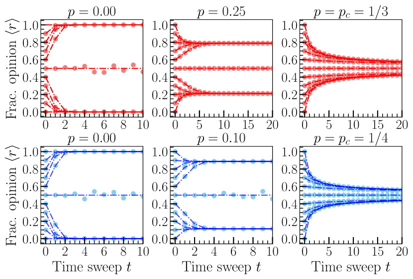
Figure 1: The comparison between analytical treatment and numerical simulation for the model with independence (red) and anticonformity (blue) for various values of probability $p$. As seen, at $p=0$, all data $r_{0}$ evolve to a complete consensus with $r=1$ and $r=0$. At $0<p<p_{c}$, all data evolve to two stable $r_{st}$, and at $p=p_{c}$ all data evolve to $r=1/2$ (disordered state). The population size is $N=10^{4}$, and each data point averages over $300$ independent realizations.

3.2 Phase diagram and critical exponents

The order-disorder phase transition of the model can be analyzed by determining the stationary condition of Eq. (12), where $dr/dt=0$. For the model with independence on the complete graph, the stationary results are as follows:

$$r_{1}=1/2,\,r_{2,3}=\dfrac{1}{2}\left[1\pm\left(\dfrac{1-3p}{1-p}\right)^{1/2}\right]\Rightarrow m_{2,3}=\pm\left(\dfrac{1-3p}{1-p}\right)^{1/2},$$ (21)

where $r_{1}$ corresponds to $r=1/2$, while $r_{2,3}$ represents two additional stationary values. The critical point occurs at $p_{c}=1/3$, where $m_{2,3}=0$. Additionally, for the model with anticonformity, the stationary condition for the fraction opinion $r$ yields:

$$r_{1}=1/2,\,r_{2,3}=\dfrac{1}{2}\left[1\pm\left(1-4p\right)^{1/2}\right]\Rightarrow m_{2,3}=\pm\left(1-4p\right)^{1/2}.$$ (22)

In this case, $r_{1}$ corresponds to $r=1/2$, and $r_{2,3}$ represents two additional stationary values. The critical point is $p_{c}=1/4$. Both sets of equations, Eqs. (21) and (22), can be expressed as power laws in terms of $p$, where $m\sim(p-p_{c})^{\beta}$. In these equations, $\beta$ takes the value $1/2$, typical of the critical exponent corresponding to the magnetization of the mean-field Ising model [40].

As mentioned earlier, the topology of the complete graph can be approximated using a mean-field formulation. Monte Carlo simulations were conducted with a large population size $N=10^{6}$ to confirm the analytical results, as shown in Fig. 2 (a). The analytical results closely match the Monte Carlo simulation results, demonstrating that both models with independence and anticonformity undergo a continuous phase transition. Furthermore, Fig. 2 (b) and (c) illustrate the effective potential in Eqs. (23) and (24), respectively. These plots reveal the following behaviors, namely; for $p<p_{c}$, the potential is bistable, for $p>p_{c}$, the potential is monostable and at $p=p_{c}$, the transition occurs between bistable and monostable, indicating the critical point of the model. These results provide a comprehensive understanding of the phase diagram and critical behavior of the model on the complete graph.

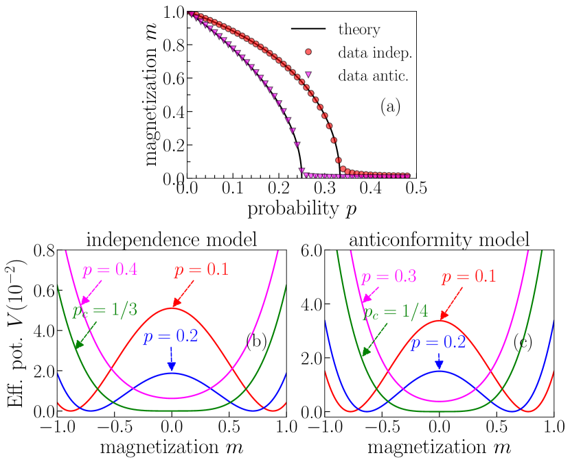
Figure 2: Phase diagram of the model on the complete graph with both independence and anticonformity. Analytical results in Eqs. (21) and (22) are compared with Monte Carlo simulation data. The models exhibit continuous phase transitions with critical points at $p_{c}=1/3$ and $p_{c}=1/4$, respectively. Panels (b) and (c) display the effective potential in Eqs. (23) and (24), respectively, illustrating bistable and monostable behaviors for different $p$ values.

Another approach to analyzing the order-disorder phase transition of the model is to consider the effective potential, which can be obtained through integration. Traditionally, the effective potential is derived from the effective force $V(r)_{\text{eff}}=-\int f(r)_{\text{eff}}\,\mathrm{d}r$, where $f(r)_{\text{eff}}=\rho^{+}(r)-\rho^{-}(r)$ represents the force driving the opinion change during the dynamics process. For the model with independence on the complete graph, the effective potential is given by:

$$V(m,p)_{\text{indep.}}=3\left(1-p\right)^{-1}\left(1-3p-\left(1-p\right)m^{2}\right)^{2}/32.$$ (23)

Moreover, for the model with anticonformity, the effective potential is expressed as:

$$V(m,p)_{\text{antic.}}=-3\left(1-4p-m^{2}\right)^{2}/32.$$ (24)

Plot of Eqs. (23) and (24) are exhibited in panels (b) and (c) of Fig. 2. One can see for both potentials, there are bistable states for $p<p_{c}$, the transition bistable-monostable at $p=p_{c}$, and the system is in a monostable for $p>p_{c}$, indicating the model undergoes a continuous phase transition at $p_{c}$.

The critical point of the model can also be analyzed using Landau’s theory. According to Landau’s theory, the potential can be expanded by the magnetization $m$ as $V=\sum_{i}V_{i}m^{i}$, where $V_{i}$ generally depends on thermodynamic parameters [41]. In this model, $V_{i}$ can depend on the noise parameters of the model, such as probability independence and anticonformity $p$. The Landau potential $V$ is symmetric under inversion of the order parameter $m\to-m$. Therefore, only even terms of the potential are considered. Thus, the simplified Landau potential takes the form:

$$V=V_{0}+V_{2}m^{2}+V_{4}m^{4}+V_{6}m^{6}\cdots$$ (25)

It is sufficient to know the terms $V_{2}$ and $V_{4}$ to analyze the model’s phase transition using the potential V. The critical point can be determined by setting $V_{2}=0$, while the nature of the phase transition is determined by $V_{4}(p_{c})$, where $V_{4}(p_{c})\geq 0$ indicates a continuous phase transition, and $V_{4}(p_{c})<0$ indicates a discontinuous phase transition. Comparing Eq. (25) with Eqs. (23) and (24), we can determine $V_{2}$ and $V_{4}$ for both the model with independence and the model with anticonformity. For the model with independence, we obtain $V_{2}(p)=3\left(1-3,p\right)/8$ and $V_{4}(p)=9\left(1-p\right)/4$. For the model with anticonformity, we obtain $V_{2}(p)=-3\left(1-4p\right)/8$ and $V_{4}(p)=9/4$. As a result, the critical points $p_{c}$ are consistent with the values obtained from the equilibrium analysis: $p_{c}=1/3$ for the model with independence and $p_{c}=1/4$ for the model with anticonformity. Furthermore, $V_{4}(p_{c})\geq 0$ for both models confirms that they undergo a continuous phase transition. This analysis provides an additional perspective on the phase transition behavior of the model, showing agreement with the previously obtained critical points and the nature of the transitions.

To numerically estimate the model’s critical point and critical exponents, finite-size scaling relations in Eqs. (2)-(7) are employed. The population size $N$ is varied in the range of $2000~{}\text{to}~{}10000$ to compute the magnetization $m$, susceptibility $\chi$, and Binder cumulant $U$ as shown in Fig. 3. We take for each data point is averaged over $10^{5}$ independent realizations to obtain good results. In the inset graphs of Fig. 3, normal plots are presented, while the main graphs show the scaling plots of the model. The critical point of the model is determined using the Binder method, which involves observing the crossing of lines between the Binder cumulant $U$ and the probability of anticonformity $p$. In this case, the critical point is estimated to be $p_{c}\approx 0.25$ (inset panel a), which agrees with the analytical result in Eq. (22).

The main graphs of Fig. 3 display the scaling plots of the model. The best critical exponents that result in the best collapse of all data points are $\beta\approx 0.5,\nu\approx 2.0,$ and $\gamma\approx 1.0.$. Here, $\nu$ is the critical exponent corresponding to the critical dimension $d_{c}=4$, and the effective exponent $\nu$ is $1/2$. Consequently, $\nu=d_{c}\nu^{\prime}=2$ is obtained numerically. These critical exponents satisfy the identity relation $\nu d=2\beta+\gamma$’, and they indicate that the universality class of the model belongs to the mean-field Ising universality class [40]. It is important to note that the same critical exponents are obtained for the model with independence, suggesting that both models with independence and anticonformity are identical. These models are also identical to well-known models in the field, such as the Sznajd and kinetics exchange models. This finite-size scaling analysis provides robust numerical evidence supporting the model’s critical point and exponents, corroborating the analytical findings and classifying the model within the mean-field Ising universality class.

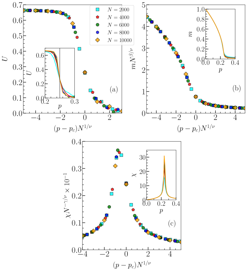
Figure 3: Monte Carlo simulation result of the model for the order parameter $m$, susceptibility $\chi$, and Binder cumulant $U$ (inset graphs) for several population sizes $N$. The critical point is obtained from the crossing lines Binder cumulant $U$ versus probability $p$ that occurs at $p=p_{c}\approx 0.25$ (inset graph of the panel (a)). This critical point confirms the analytical result in Eq. (22). The best critical exponents that make all data collapse near the critical point $p_{c}$ are $\beta\approx 0.5,\nu\approx 2.0,$ and $\gamma\approx 1.0$ (see the main graph) that indicate the model belongs to the mean-field Ising model [40].

3.3 The model on the 2-D lattice

We examined several population sizes, denoted as $N=L^{2}$, where $L$ assumes values of $32,45,64,100,150$, and $200$, to investigate the model’s critical point and critical exponents thoroughly. The numerical results, specifically pertaining to the order parameter $m$, susceptibility $\chi$, and Binder cumulant $U$, are presented in Fig. 4. The critical point, signifying the point at which the model undergoes a continuous phase transition, is identified as $p_{c}\approx 0.106$ (as seen in the inset panel of Fig. 4 (a)). We determined the optimal critical exponents that result in the best data collapse by utilizing the finite-size scaling relations detailed in Eqs. (2)-(5). These critical exponents are approximately $\beta\approx 2.0,\gamma\approx 1.75$, and $\nu\approx 0.125$. Notably, these values indicate that the model is akin to the Sznajd model [30, 42] and shares characteristics with the universality class of the two-dimensional Ising model [40].

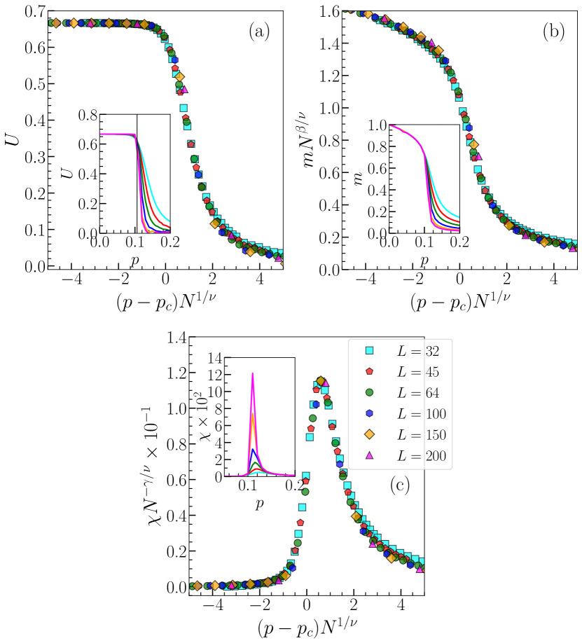
Figure 4: (Main panel) Scaling plot of the Binder cumulant $U$ (panel (a)), the order parameter $m$ (panel (b)), and the susceptibility (panel (c). These results are derived from extensive numerical simulations. Notably, for a critical point at approximately $p_{c}\approx 0.106$, we observe that all data, with population sizes $N=L^{2}$, exhibit a remarkable collapse. The associated critical exponents are estimated to be $\nu\approx 2.0$, $\gamma\approx 1.75$, and $\beta\approx 0.125$. The critical point $p_{c}$ is determined by identifying the intersection of the curves for the Binder cumulant $U$ as a function of the independence probability $p$ (inset panel (a)). These results align with the critical exponents of the two-dimensional Ising model universality class. It is important to note that all inset panels present data in a normal plot format, and each data point results from averaging over $3\times 10^{6}$ independent realizations.

Similarly, we extended our analysis to the model with anticonformity, and our findings reveal that this model also experiences a continuous phase transition. The critical point for the model with anticonformity is approximately $p_{c}\approx 0.062$, as shown in Fig. 5. Remarkably, our investigations yielded identical critical exponents for this model, specifically $\beta\approx 0.125,\nu\approx 2.0$ and $\gamma\approx 1.75$. These shared critical exponents indicate that both the model with independence and the model with anticonformity exhibit analogous behavior, suggesting that they belong to the same universality class. Our results align these models with the two-dimensional Ising universality class. Furthermore, the critical exponents for both models adhere to the identity relation $\nu d=2\beta+\gamma$.

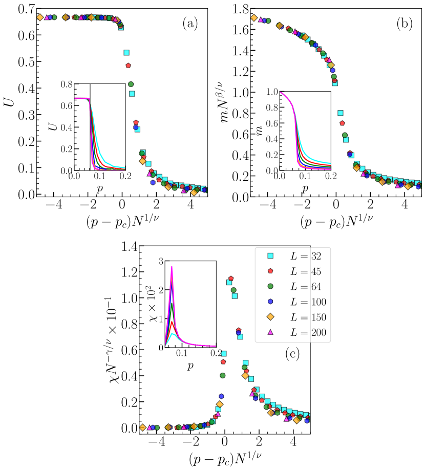
Figure 5: (Main panel) Scaling plots for the model with anticonformity: the Binder cumulant $U$ [panel (a)], the order parameter $m$ [panel (b)], and the susceptibility $\chi$ [panel (c)]. These results have been obtained through extensive numerical simulations. Notably, for a critical point located at approximately $p_{c}\approx 0.062$, we observe a remarkable collapse of all data sets with population sizes $N=L^{2}$. The associated critical exponents are estimated to be $\nu\approx 2.0$, $\gamma\approx 1.75$, and $\beta\approx 0.125$. The critical point $p_{c}$ is determined through the intersection of curves representing the Binder cumulant $U$ as a function of the independence probability $p$ (inset panel (a)). These results are consistent with the critical exponents characterizing the universality class of the two-dimensional Ising model. It is important to note that all inset panels present data in a normal plot format, and each data point results from averaging over $3\times 10^{6}$ independent realizations.

3.4 The model on the 3-D lattice

We conducted investigations using various population sizes $N=L^{3}$, with linear dimensions $L=15,20,25,30,35$. Each data point represents an average of over $10^{6}$ independent realizations. The numerical results for the model featuring independence are presented in Fig. 6. In panel (a), we observe that at $p=0.0$, the system exists in an ordered state characterized by $m=1.0$. In contrast, the magnetization decreases to zero at a small $p=0.01$, signifying a disordered state. The inset graph visually illustrates the magnetization $m$ at equilibrium for $p=0.0$ and $p=0.01$. However, relying solely on the magnetization data makes it challenging to determine whether the model undergoes an order-disorder phase transition. Nonetheless, we gain more insight into this by examining the Binder cumulant $U$, as depicted in panel (b). Notably, there are no intersections between the curves of Binder cumulant $U$ and the probability of independence $p$, which suggests the absence of an order-disorder phase transition in this model. See the inset graph for further clarity.

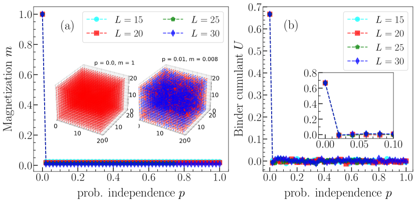
Figure 6: The numerical results for the order parameter $m$ [panel (a)] and Binder cumulant $U$ [panel (b)] are presented for the model with independence on the three-dimensional square lattice. Notably, the order parameter $m$ diminishes to zero at a low independence probability of $p=0.01$, indicating the absence of an order-disorder phase transition in this model. Furthermore, the data depicting Binder cumulant $U$ as a function of probability $p$ reveals a lack of intersections between the curves. For a clearer illustration, please refer to the inset graph.

Our analysis of the model defined on the 3-D square lattice reveals that it undergoes a second-order phase transition with a critical point at $p_{c}\approx 0.268$, as illustrated in Fig. 7. By employing finite-size scaling relations, detailed in Eqs. (2)-(5), we have determined the best-fitting critical exponents, yielding values of $\beta\approx 0.25$, $\nu\approx 2.0$, and $\gamma\approx 1.4$. The results suggest that this model is not in the same universality class as the three-dimensional Ising model [40]. These critical exponents are universal, as they remain consistent across various different data sets for different system sizes $N$.

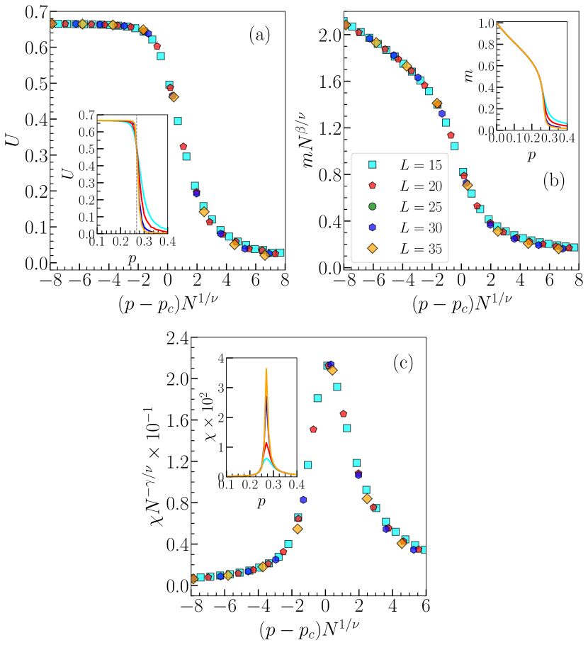
Figure 7: (Main graph) Scaling plots for the Binder cumulant $U$, order parameter $m$, and susceptibility $\chi$ for the model with anticonformity on the 3-D lattice. Based on the results, the model undergoes a continuous phase transition with a critical point at $p_{c}\approx 0.268$ (see inset figure (a)). Additionally, we determine the best critical exponents as $\beta\approx 0.25,\nu\approx 2.0$, and $\gamma\approx 1.40$, leading to the collapse of all data points around the critical point, as indicated. Each data point averages $10^{6}$ independent realizations.

3.5 The model on the heterogeneous networks

Compared to the aforementioned homogeneous networks, the W-S, A-B, and E-R networks are more representative of real social networks [34, 43]. These three networks have been extensively studied in various network research and applied to a wide range of social phenomena, including applications in the field of medicine [44]. In this section, we considered these three heterogeneous networks, visually represented in Fig. 8.

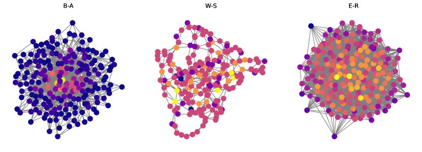
Figure 8: Three heterogeneous networks, namely the Watts-Strogatz (W-S) network, Barabasi-Albert (A-B) network, and Erdos-Renyi (E-R) network, were generated using networkx [45]. The population size or number of nodes, denoted as $N=200$, and all networks have a minimum degree of connectivity set to $2$.

Within these networks, we selected an agent possessing at least two randomly chosen nearest neighbors, as illustrated in Fig. 9.

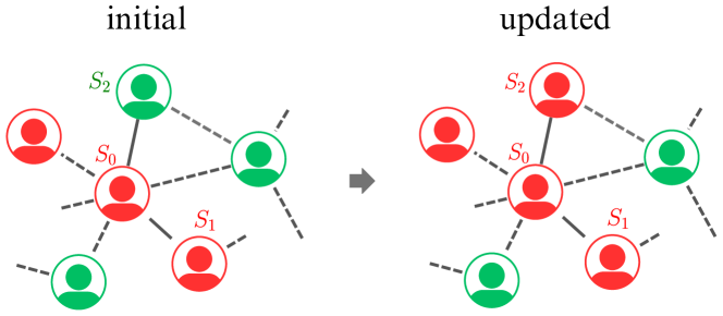
Figure 9: Illustration of the selection of three agents at random (initial and updated state): agent $S_{0}$ is initially chosen, followed by the random selection of its two neighboring agents, $S_{1}$ and $S_{2}$ (solid edges), who interact based on the majority rule. The red and green colors represent agents with opinions or states of “up” and “down,” respectively.

The three agents interacted with each other according to the model’s algorithm. We assigned varying node degrees in all networks, with the minimum node degree being $2$. In other words, each agent has at least two nearest neighbors. The population size was $N=3000$, and each data point was an average of $10^{5}$ independent realizations. In this part, we exclusively focus on analyzing whether or not the model undergoes a continuous phase transition. Therefore, we do not seek critical points and critical exponents as in the previously discussed homogeneous networks. Our numerical results for the order parameter $m$ are presented in Fig. 10. It can be observed that when $p=0$, the system is in a state of complete order. This situation arises because all nodes have at least two nearest neighbors, allowing them to interact with each other following the majority rule. It is also shown that the model undergoes a continuous phase transition in all three networks, each with different critical points (not specified in this paper). Other types of phase transitions, such as discontinuous phase transitions, can also occur for groups with a larger number of the group of agents, for example, $7$, or under different scenarios.

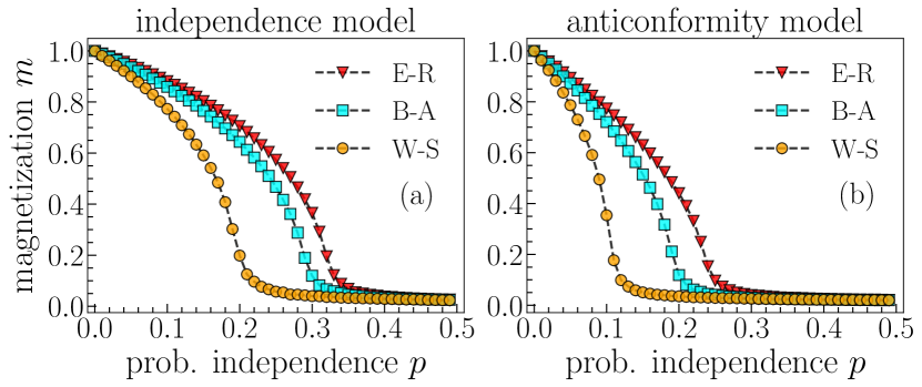
Figure 10: Phase diagrams illustrating the occurrence of continuous phase transitions for the models with independence and nonconformity on Barabasi-Albert (A-B), Erdos-Renyi (E-R), and Watts-Strogatz (W-S) networks. The population size is $N=5000$, and each data point represents the average of $10^{4}$ independent realizations.

To further observe the continuous phase transition in the model defined on these heterogeneous networks, we analyzed the magnetization fluctuations m versus Monte Carlo steps. The results are shown in Fig. 11. It can be seen that a bistable state of the magnetization $m$ emerges for all models on all networks, indicating that the model undergoes a continuous phase transition.

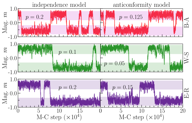
Figure 11: The Monte Carlo step for the magnetization $m$ of the model on heterogeneous networks occurs at low values of $p$. It can be observed that the magnetization exhibits fluctuations between two stable states, indicating that the model undergoes a continuous phase transition.

4 Summary and outlook

This paper delves into the disruptive social phenomena’s impact, such as independence and nonconformity, on the occurrence of phase transitions from order to disorder based on majority rule. The model’s scope encompasses homogeneous networks such as complete graphs, two-dimensional square lattices, and three-dimensional square lattices, as well as heterogeneous networks like Barabasi-Albert networks, Watts-Strogatz networks, and Erdos-Renyi networks. A probability parameter measures the likelihood of agents adopting independent or nonconformist behavior, denoted as $p$, while agents conform to the majority opinion with a probability of $(1-p)$.

Our results, analytically (for the complete graph) and through numerical simulations, indicate that the model in homogeneous networks undergoes a continuous phase transition with different critical points, as summarized in Table 1. However, we found no phase transition for the 3-D lattice model with independence. The critical exponents for the complete graph and the two-dimensional lattice model, obtained through finite-size scaling analysis, suggest that the model belongs to the same class as mean-field and 2-D Ising models. These critical exponents satisfy the scaling identity relation $\nu d=2\beta+\gamma$. Furthermore, for the model with nonconformity on the 3-D lattice, the obtained critical exponents are $\beta\approx 0.25,\nu\approx 1.40,$ and $\nu\approx 2.0$, indicating that the model does not belong to the same class as the 3-D Ising model.

Table 1: Critical exponents of the majority-rule model on regular networks.

Networks	S. Noises	Critical Point	$\beta$	$\gamma$	$\nu$
Com.-graph	Independence	$1/3$	0.5	1.0	2.0
	Anticonformity	$1/4$	0.5	1.0	2.0
2-D lattice	Independence	0.106	0.125	1.75	2.0
	Anticonformity	0.062	0.125	1.75	2.0
3-D lattice	Independence	-	-	-	-
	Anticonformity	0.268	0.25	1.40	2.0

The model defined on heterogeneous networks such as B-A, W-S, and E-R networks undergoes a continuous phase transition with distinct critical points, as demonstrated by the magnetization data versus probability $p$. This conclusion is further supported by the fluctuations in the two stable magnetic states, denoted as $m$, indicating that the model undergoes a continuous phase transition. We did not estimate the critical points of the model any further; however, based on numerical data for magnetization $m$ versus probability $p$, it is evident that the critical point of the model with nonconformity is smaller than that of the model with independence. This difference also holds consistently for models defined on complete graphs and 2-D lattices. From these data, we can assert that models with nonconformity have a greater tendency to undergo an order-disorder phase transition.

From a social systems perspective, we can assert that complete consensus is achieved when no independent or nonconformist agents are present. Below the critical point is a coexistence of majority and minority opinions. However, at $p\geq p_{c}$, the system reaches an equilibrium state akin to a deadlock. After comparing the critical points of the independence and nonconformity models, it becomes evident that the model with nonconformity exhibits a lower critical point than its independence counterpart. These results imply that systems containing nonconformist agents tend to reach a stalemate state more than systems containing independent agents. These findings are consistent with what we previously reported in our prior study [31]. Of course, differences in such phenomena are highly dependent on the applied model or scenario.

CRediT authorship contribution statement

D. A. Mulya and R. Muslim: Conceptualization, Methodology, Writing, Software, Formal analysis, Validation, Writing, Visualization, Review & editing. R. Muslim: Main Contributor & Supervision. All authors read and reviewed the paper.

Declaration of Interests

The contributors declare that they have no apparent competing business or personal connections that might have appeared to have influenced the reported work.

References

- [1] S. Galam, Sociophysics: A Physicist’s Modeling of Psycho-political Phenomena, Springer-Verlag, New York, 2012.
- [2] C. Castellano, S. Fortunato, V. Loreto, Statistical physics of social dynamics, Rev. Mod. Phys. 81 (2009) 591.
- [3] S. Galam, Sociophysics: a personal testimony, Physica A: Statistical Mechanics and its Applications 336 (1-2) (2004) 49–55.
- [4] P. Sen, B. K. Chakrabarti, Sociophysics: an introduction, Oxford, Oxford University Press, 2014.
- [5] S. Galam, Majority rule, hierarchical structures, and democratic totalitarianism: A statistical approach, Journal of Mathematical Psychology 30 (4) (1986) 426–434.
- [6] M. Mobilia, S. Redner, Majority versus minority dynamics: Phase transition in an interacting two-state spin system, Phys. Rev. E 68 (2003) 046106.
- [7] P. L. Krapivsky, S. Redner, Dynamics of majority rule in two-state interacting spin systems, Phys. Rev. Lett. 90 (2003) 238701.
- [8] S. Biswas, P. Sen, Model of binary opinion dynamics: Coarsening and effect of disorder, Physical Review E 80 (2) (2009) 027101.
- [9] K. Sznajd-Weron, J. Sznajd, Opinion evolution in closed community, Int. J. Mod. Phys. C 11 (2000) 1157–1165.
- [10] K. Sznajd-Weron, J. Sznajd, T. Weron, A review on the sznajd model—20 years after, Physica A: Statistical Mechanics and its Applications 565 (2021) 125537.
- [11] G. Deffuant, D. Neau, F. Amblard, G. Weisbuch, Mixing beliefs among interacting agents, Advances in Complex Systems 3 (3) (2000) 87–98.
- [12] G. Weisbuch, G. Deffuant, F. Amblard, J.-P. Nadal, Meet, discuss, and segregate!, Complexity 7 (3) (2002) 55–63.
- [13] S. E. Asch, Studies of independence and conformity: I. a minority of one against a unanimous majority., Psychological monographs: General and applied 70 (9) (1956) 1.
- [14] R. H. Willis, Two dimensions of conformity-nonconformity, Sociometry (1963) 499–513.
- [15] R. H. Willis, Conformity, independence, and anticonformity, Hum. Relat. 18 (1965) 373–388.
- [16] G. MacDonald, P. R. Nail, D. A. Levy, Expanding the scope of the social response context model, Basic Appl. Soc. Psych. 26 (2004) 77–92.
- [17] P. R. Nail, G. MacDonald, On the development of the social response context model, in: The science of social influence: Advances and future progress, New York, Psychology Press, 2007, pp. 193–221.
- [18] K. Sznajd-Weron, M. Tabiszewski, A. M. Timpanaro, Phase transition in the sznajd model with independence, Europhys. Lett. 96 (2011) 48002.
- [19] P. Nyczka, K. Sznajd-Weron, Anticonformity or independence?—insights from statistical physics, J. Stat. Phys. 151 (2013) 174–202.
- [20] M. A. Javarone, Social influences in opinion dynamics: the role of conformity, Physica A: Statistical Mechanics and its Applications 414 (2014) 19–30.
- [21] N. Crokidakis, P. M. C. de Oliveira, Inflexibility and independence: Phase transitions in the majority-rule model, Phys. Rev. E 92 (2015) 062122.
- [22] A. Chmiel, K. Sznajd-Weron, Phase transitions in the q-voter model with noise on a duplex clique, Physical Review E 92 (5) (2015) 052812.
- [23] A. Abramiuk, J. Pawłowski, K. Sznajd-Weron, Is independence necessary for a discontinuous phase transition within the q-voter model?, Entropy 21 (5) (2019) 521.
- [24] R. Muslim, R. Anugraha, S. Sholihun, M. F. Rosyid, Phase transition of the sznajd model with anticonformity for two different agent configurations, Int. J. Mod. Phys. C 31 (2020) 2050052.
- [25] B. Nowak, B. Stoń, K. Sznajd-Weron, Discontinuous phase transitions in the multi-state noisy q-voter model: quenched vs. annealed disorder, Scientific Reports 11 (1) (2021) 1–13.
- [26] J. Civitarese, External fields, independence, and disorder in q-voter models, Physical Review E 103 (1) (2021) 012303.
- [27] R. Muslim, R. Anugraha, S. Sholihun, M. F. Rosyid, Phase transition and universality of the three-one spin interaction based on the majority-rule model, International Journal of Modern Physics C 32 (09) (2021) 2150115.
- [28] R. Muslim, M. J. Kholili, A. R. Nugraha, Opinion dynamics involving contrarian and independence behaviors based on the sznajd model with two-two and three-one agent interactions, Physica D: Nonlinear Phenomena 439 (2022) 133379.
- [29] R. Muslim, H. Lugo H, Effect of social behaviors in the opinion dynamics -voter model, arXiv preprint arXiv:2307.14548 (2023).
- [30] A. Azhari, R. Muslim, D. A. Mulya, H. Indrayani, C. A. Wicaksana, A. Rizki, Independence role in the generalized sznajd model, arXiv preprint arXiv:2309.13309 (2023).
- [31] R. Muslim, S. A. Wella, A. R. Nugraha, Phase transition in the majority rule model with the nonconformist agents, Physica A: Statistical Mechanics and its Applications 608 (2022) 128307.
- [32] A. L. Oestereich, M. A. Pires, S. M. Duarte Queirós, N. Crokidakis, Phase transition in the galam’s majority-rule model with information-mediated independence, Physics 5 (3) (2023) 911–922.
- [33] D. J. Watts, S. H. Strogatz, Collective dynamics of ‘small-world’networks, nature 393 (6684) (1998) 440–442.
- [34] R. Albert, A.-L. Barabási, Statistical mechanics of complex networks, Reviews of modern physics 74 (1) (2002) 47.
- [35] P. ERDdS, A. R&wi, On random graphs i, Publ. math. debrecen 6 (290-297) (1959) 18.
- [36] M. E. Fisher, The theory of equilibrium critical phenomena, Reports on progress in physics 30 (2) (1967) 615.
- [37] R. B. Cialdini, N. J. Goldstein, Social influence: Compliance and conformity, Annu. Rev. Psychol. 55 (2004) 591–621.
- [38] K. Binder, Finite size scaling analysis of ising model block distribution functions, Z. Phys. B: Condens. Matter 43 (1981) 119–140.
- [39] R. Muslim, R. A. NQZ, M. A. Khalif, Mass media and its impact on opinion dynamics of the nonlinear -voter model, arXiv preprint arXiv:2305.06053 (2023).
- [40] H. E. Stanley, Phase transitions and critical phenomena, Vol. 7, Clarendon Press, Oxford, 1971.
- [41] L. D. Landau, On the theory of phase transitions, Zh. Eksp. Teor. Fiz. 7 (1937) 19–32.
- [42] M. Calvelli, N. Crokidakis, T. J. Penna, Phase transitions and universality in the sznajd model with anticonformity, Physica A: Statistical Mechanics and its Applications 513 (2019) 518–523.
- [43] M. Newman, Networks, Oxford university press, 2018.
- [44] D. L. Barabási, G. Bianconi, E. Bullmore, M. Burgess, S. Chung, T. Eliassi-Rad, D. George, I. A. Kovács, H. Makse, T. E. Nichols, et al., Neuroscience needs network science, Journal of Neuroscience 43 (34) (2023) 5989–5995.
- [45] A. Hagberg, P. Swart, D. S Chult, Exploring network structure, dynamics, and function using networkx, Tech. rep., Los Alamos National Lab.(LANL), Los Alamos, NM (United States) (2008).