Time-LLM: Time Series Forecasting
by Reprogramming Large Language Models

Abstract

Time series forecasting holds significant importance in many real-world dynamic systems and has been extensively studied. Unlike natural language process (NLP) and computer vision (CV), where a single large model can tackle multiple tasks, models for time series forecasting are often specialized, necessitating distinct designs for different tasks and applications. While pre-trained foundation models have made impressive strides in NLP and CV, their development in time series domains has been constrained by data sparsity. Recent studies have revealed that large language models (LLMs) possess robust pattern recognition and reasoning abilities over complex sequences of tokens. However, the challenge remains in effectively aligning the modalities of time series data and natural language to leverage these capabilities. In this work, we present Time-LLM, a reprogramming framework to repurpose LLMs for general time series forecasting with the backbone language models kept intact. We begin by reprogramming the input time series with text prototypes before feeding it into the frozen LLM to align the two modalities. To augment the LLM’s ability to reason with time series data, we propose Prompt-as-Prefix (PaP), which enriches the input context and directs the transformation of reprogrammed input patches. The transformed time series patches from the LLM are finally projected to obtain the forecasts. Our comprehensive evaluations demonstrate that Time-LLM is a powerful time series learner that outperforms state-of-the-art, specialized forecasting models. Moreover, Time-LLM excels in both few-shot and zero-shot learning scenarios. The code is made available at https://github.com/KimMeen/Time-LLM

1 Introduction

Time series forecasting is a critical capability across many real-world dynamic systems (Jin et al., 2023a), with applications ranging from demand planning (Leonard, 2001) and inventory optimization (Li et al., 2022) to energy load forecasting (Liu et al., 2023a) and climate modeling (Schneider & Dickinson, 1974). Each time series forecasting task typically requires extensive domain expertise and task-specific model designs. This stands in stark contrast to foundation language models like GPT-3 (Brown et al., 2020), GPT-4 (OpenAI, 2023), Llama (Touvron et al., 2023), inter alia, which can perform well on a diverse range of NLP tasks in a few-shot or even zero-shot setting.

Pre-trained foundation models, such as large language models (LLMs), have driven rapid progress in computer vision (CV) and natural language processing (NLP). While time series modeling has not benefited from the same significant breakthroughs, LLMs’ impressive capabilities have inspired their application to time series forecasting (Jin et al., 2023b). Several desiderata exist for leveraging LLMs to advance forecasting techniques: Generalizability. LLMs have demonstrated a remarkable capability for few-shot and zero-shot transfer learning (Brown et al., 2020). This suggests their potential for generalizable forecasting across domains without requiring per-task retraining from scratch. In contrast, current forecasting methods are often rigidly specialized by domain. Data efficiency. By leveraging pre-trained knowledge, LLMs have shown the ability to perform new tasks with only a few examples. This data efficiency could enable forecasting for settings where historical data is limited. In contrast, current methods typically require abundant in-domain data. Reasoning. LLMs exhibit sophisticated reasoning and pattern recognition capabilities (Mirchandani et al., 2023; Wang et al., 2023; Chu et al., 2023). Harnessing these skills could allow making highly precise forecasts by leveraging learned higher-level concepts. Existing non-LLM methods are largely statistical without much innate reasoning. Multimodal knowledge. As LLM architectures and training techniques improve, they gain more diverse knowledge across modalities like vision, speech, and text (Ma et al., 2023). Tapping into this knowledge could enable synergistic forecasting that fuses different data types. Conventional tools lack ways to jointly leverage multiple knowledge bases. Easy optimization. LLMs are trained once on massive computing and then can be applied to forecasting tasks without learning from scratch. Optimizing existing forecasting models often requires significant architecture search and hyperparameter tuning (Zhou et al., 2023b). In summary, LLMs offer a promising path to make time series forecasting more general, efficient, synergistic, and accessible compared to current specialized modeling paradigms. Thus, adapting these powerful models for time series data can unlock significant untapped potential.

The realization of the above benefits hinges on the effective alignment of the modalities of time series data and natural language. However, this is a challenging task as LLMs operate on discrete tokens, while time series data is inherently continuous. Furthermore, the knowledge and reasoning capabilities to interpret time series patterns are not naturally present within LLMs’ pre-training. Therefore, it remains an open challenge to unlock the knowledge within LLMs in activating their ability for general time series forecasting in a way that is accurate, data-efficient, and task-agnostic.

In this work, we propose Time-LLM, a reprogramming framework to adapt large language models for time series forecasting while keeping the backbone model intact. The core idea is to reprogram the input time series into text prototype representations that are more naturally suited to language models’ capabilities. To further augment the model’s reasoning about time series concepts, we introduce Prompt-as-Prefix (PaP), a novel idea in enriching the input time series with additional context and providing task instructions in the modality of natural language. This provides declarative guidance about desired transformations to apply to the reprogrammed input. The output of the language model is then projected to generate time series forecasts. Our comprehensive evaluation demonstrates that large language models can act as effective few-shot and zero-shot time series learners when adopted through this reprogramming approach, outperforming specialized forecasting models. By leveraging LLMs’ reasoning capability while keeping the models intact, our work points the way toward multimodal foundation models that can excel on both language and sequential data tasks. Our proposed reprogramming framework offers an extensible paradigm for imbuing large models with new capabilities beyond their original pre-training. Our main contributions in this work can be summarized as follows:

• We introduce a novel concept of reprogramming large language models for time series forecasting without altering the pre-trained backbone model. In doing so, we show that forecasting can be cast as yet another “language” task that can be effectively tackled by an off-the-shelf LLM.

• We propose a new framework, Time-LLM, which encompasses reprogramming the input time series into text prototype representations that are more natural for the LLM, and augmenting the input context with declarative prompts (e.g., domain expert knowledge and task instructions) to guide LLM reasoning. Our technique points towards multimodal foundation models excelling in both language and time series.

• Time-LLM consistently exceeds state-of-the-art performance in mainstream forecasting tasks, especially in few-shot and zero-shot scenarios. Moreover, this superior performance is achieved while maintaining excellent model reprogramming efficiency. Thus, our research is a concrete step in unleashing LLMs’ untapped potential for time series and perhaps other sequential data.

2 Related Work

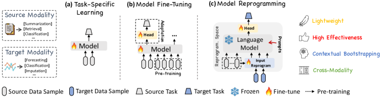
Figure 1: Schematic illustration of reprogramming large language models (LLMs) in comparison of (a) task-specific learning and (b) model fine-tuning. Our proposal investigates and demonstrates (c) how to effectively reprogram open-sourced LLMs as powerful time series learners where well-developed time series pre-trained models are not readily available.

Task-specific Learning. Most time series forecasting models are crafted for specific tasks and domains (e.g., traffic prediction), and trained end-to-end on small-scale data. An illustration is in Figure 1(a). For example, ARIMA models are designed for univariate time series forecasting (Box et al., 2015), LSTM networks are tailored for sequence modeling (Hochreiter & Schmidhuber, 1997), and temporal convolutional networks (Bai et al., 2018) and transformers (Wen et al., 2023) are developed for handling longer temporal dependencies. While achieving good performance on narrow tasks, these models lack versatility and generalizability to diverse time series data.

In-modality Adaptation. Relevant research in CV and NLP has demonstrated the effectiveness of pre-trained models that can be fine-tuned for various downstream tasks without the need for costly training from scratch (Devlin et al., 2018; Brown et al., 2020; Touvron et al., 2023). Inspired by these successes, recent studies have focused on the development of time series pre-trained models (TSPTMs). The first step among them involves time series pre-training using different strategies like supervised (Fawaz et al., 2018) or self-supervised learning (Zhang et al., 2022b; Deldari et al., 2022; Zhang et al., 2023). This allows the model to learn representing various input time series. Once pre-trained, it can be fine-tuned on similar domains to learn how to perform specific tasks (Tang et al., 2022). An example is in Figure 1(b). The development of TSPTMs leverages the success of pre-training and fine-tuning in NLP and CV but remains limited on smaller scales due to data sparsity.

Cross-modality Adaptation. Building on in-modality adaptation, recent work has further explored transferring knowledge from powerful pre-trained foundations models in NLP and CV to time series modeling, through techniques such as multimodal fine-tuning (Yin et al., 2023) and model reprogramming (Chen, 2022). Our approach aligns with this category; however, there is limited pertinent research available on time series. An example is Voice2Series (Yang et al., 2021), which adapts an acoustic model (AM) from speech recognition to time series classification by editing a time series into a format suitable for the AM. Recently, Chang et al. (2023) proposes LLM4TS for time series forecasting using LLMs. It designs a two-stage fine-tuning process on the LLM - first supervised pre-training on time series, then task-specific fine-tuning. Zhou et al. (2023a) leverages pre-trained language models without altering their self-attention and feedforward layers. This model is fine-tuned and evaluated on various time series analysis tasks and demonstrates comparable or state-of-the-art performance by transferring knowledge from natural language pre-training. Distinct from these approach, we neither edit the input time series directly nor fine-tune the backbone LLM. Instead, as illustrated in Figure 1(c), we propose reprogramming time series with the source data modality along with prompting to unleash the potential of LLMs as effective time series machines.

3 Methodology

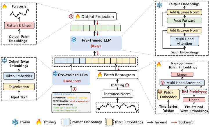
Figure 2: The model framework of Time-LLM. Given an input time series, we first tokenize and embed it via patching along with a customized embedding layer. These patch embeddings are then reprogrammed with condensed text prototypes to align two modalities. To augment the LLM’s reasoning ability, additional prompt prefixes are added to the input to direct the transformation of input patches. The output patches from the LLM are projected to generate the forecasts.

Our model architecture is depicted in Figure 2. We focus on reprogramming an embedding-visible language foundation model, such as Llama (Touvron et al., 2023) and GPT-2 (Radford et al., 2019), for general time series forecasting without requiring any fine-tuning of the backbone model. Specifically, we consider the following problem: given a sequence of historical observations $\mathbf{X}\in\mathbb{R}^{N\times T}$ consisting of $N$ different 1-dimensional variables across $T$ time steps, we aim to reprogram a large language model $f(\cdot)$ to understand the input time series and accurately forecast the readings at $H$ future time steps, denoted by $\hat{\mathbf{Y}}\in\mathbb{R}^{N\times H}$, with the overall objective to minimize the mean square errors between the ground truths $\mathbf{Y}$ and predictions, i.e., $\frac{1}{H}\sum_{h=1}^{H}||\hat{\mathbf{Y}}_{h}-\mathbf{Y}_{h}||^{2}_{F}$.

Our method encompasses three main components: (1) input transformation, (2) a pre-trained and frozen LLM, and (3) output projection. Initially, a multivariate time series is partitioned into $N$ univariate time series, which are subsequently processed independently (Nie et al., 2023). The $i$-th series is denoted as $\mathbf{X}^{(i)}\in\mathbb{R}^{1\times T}$, which undergoes normalization, patching, and embedding prior to being reprogrammed with learned text prototypes to align the source and target modalities. Then, we augment the LLM’s time series reasoning ability by prompting it together with reprogrammed patches to generate output representations, which are projected to the final forecasts $\hat{\mathbf{Y}}^{(i)}\in\mathbb{R}^{1\times H}$.

We note that only the parameters of the lightweight input transformation and output projection are updated, while the backbone language model is frozen. In contrast to vision-language and other multimodal language models, which usually fine-tune with paired cross-modality data, Time-LLM is directly optimized and becomes readily available with only a small set of time series and a few training epochs, maintaining high efficiency and imposing fewer resource constraints compared to building large domain-specific models from scratch or fine-tuning them. To further reduce memory footprints, various off-the-shelf techniques (e.g., quantization) can be seamlessly integrated for slimming Time-LLM.

3.1 Model Structure

Input Embedding. Each input channel $\mathbf{X}^{(i)}$ is first individually normalized to have zero mean and unit standard deviation via reversible instance normalization (RevIN) in mitigating the time series distribution shift (Kim et al., 2021). Then, we divide $\mathbf{X}^{(i)}$ into several consecutive overlapped or non-overlapped patches (Nie et al., 2023) with length $L_{p}$; thus the total number of input patches is $P=\lfloor\frac{(T-L_{p})}{S}\rfloor+2$, where $S$ denotes the horizontal sliding stride. The underlying motivations are two-fold: (1) better preserving local semantic information by aggregating local information into each patch and (2) serving as tokenization to form a compact sequence of input tokens, reducing computational burdens. Given these patches $\mathbf{X}^{(i)}_{P}\in\mathbb{R}^{P\times L_{p}}$, we embed them as $\hat{\mathbf{X}}^{(i)}_{P}\in\mathbb{R}^{P\times d_{m}}$, adopting a simple linear layer as the patch embedder to create dimensions $d_{m}$.

Patch Reprogramming. Here we reprogram patch embeddings into the source data representation space to align the modalities of time series and natural language to activate the backbone’s time series understanding and reasoning capabilities. A common practice is learning a form of “noise” that, when applied to target input samples, allows the pre-trained source model to produce the desired target outputs without requiring parameter updates. This is technically feasible for bridging data modalities that are identical or similar. Examples include repurposing a vision model to work with cross-domain images (Misra et al., 2023) or reprogramming an acoustic model to handle time series data (Yang et al., 2021). In both cases, there are explicit, learnable transformations between the source and target data, allowing for the direct editing of input samples. However, time series can neither be directly edited nor described losslessly in natural language, posing significant challenges to directly bootstrap the LLM for understanding time series without resource-intensive fine-tuning.

To close this gap, we propose reprogramming $\hat{\mathbf{X}}^{(i)}_{P}$ using pre-trained word embeddings $\mathbf{E}\in\mathbb{R}^{V\times D}$ in the backbone, where $V$ is the vocabulary size. Nevertheless, there is no prior knowledge indicating which source tokens are directly relevant. Thus, simply leveraging $\mathbf{E}$ will result in large and potentially dense reprogramming space. A simple solution is to maintain a small collection of text prototypes by linearly probing $\mathbf{E}$, denoted as $\mathbf{E^{\prime}}\in\mathbb{R}^{V^{\prime}\times D}$, where $V^{\prime}\ll V$. An illustration is in Figure 3(a). Text prototypes learn connecting language cues, e.g., “short up” (red lines) and “steady down” (blue lines), which are then combined to represent the local patch information (e.g., “short up then down steadily” for characterizing patch 5) without leaving the space where the language model is pre-trained. This approach is efficient and allows for the adaptive selection of relevant source information. To realize this, we employ a multi-head cross-attention layer. Specifically, for each head $k=\{1,\cdots,K\}$, we define query matrices $\mathbf{Q}^{(i)}_{k}=\hat{\mathbf{X}}^{(i)}_{P}\mathbf{W}^{Q}_{k}$, key matrices $\mathbf{K}^{(i)}_{k}=\mathbf{E^{\prime}}\mathbf{W}^{K}_{k}$, and value matrices $\mathbf{V}^{(i)}_{k}=\mathbf{E^{\prime}}\mathbf{W}^{V}_{k}$, where $\mathbf{W}^{Q}_{k}\in\mathbb{R}^{d_{m}\times d}$  and  $\mathbf{W}^{K}_{k},\mathbf{W}^{V}_{k}\in\mathbb{R}^{D\times d}$. Specifically, $D$ is the hidden dimension of the backbone model, and $d=\lfloor\frac{d_{m}}{K}\rfloor$. Then, we have the operation to reprogram time series patches in each attention head defined as:

$$\mathbf{Z}^{(i)}_{k}=\textsc{Attention}(\mathbf{Q}^{(i)}_{k},\mathbf{K}^{(i)}_{k},\mathbf{V}^{(i)}_{k})=\textsc{Softmax}(\frac{\mathbf{Q}^{(i)}_{k}\mathbf{K}^{(i){\top}}_{k}}{\sqrt{d_{k}}})\mathbf{V}^{(i)}_{k}.$$ (1)

By aggregating each $\mathbf{Z}^{(i)}_{k}\in\mathbb{R}^{P\times d}$ in every head, we obtain $\mathbf{Z}^{(i)}\in\mathbb{R}^{P\times d_{m}}$. This is then linearly projected to align the hidden dimensions with the backbone model, yielding $\mathbf{O}^{(i)}\in\mathbb{R}^{P\times D}$.

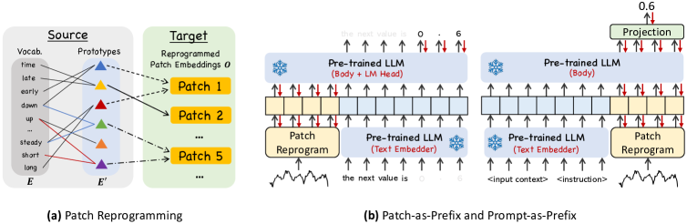
Figure 3: Illustration of (a) patch reprogramming and (b) Patch-as-Prefix versus Prompt-as-Prefix.

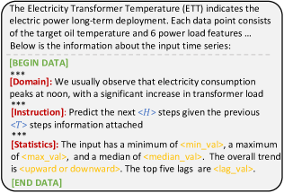
Figure 4: Prompt example. $<>$ and $<>$ are task-specific configurations and calculated input statistics.

Prompt-as-Prefix. Prompting serves as a straightforward yet effective approach task-specific activation of LLMs (Yin et al., 2023). However, the direct translation of time series into natural language presents considerable challenges, hindering both the creation of instruction-following datasets and the effective utilization of on-the-fly prompting without performance compromise (Xue & Salim, 2022). Recent advancements indicate that other data modalities, such as images, can be seamlessly integrated as the prefixes of prompts, thereby facilitating effective reasoning based on these inputs (Tsimpoukelli et al., 2021). Motivated by these findings, and to render our approach directly applicable to real-world time series, we pose an alternative question: can prompts act as prefixes to enrich the input context and guide the transformation of reprogrammed time series patches? We term this concept as Prompt-as-Prefix (PaP) and observe that it significantly enhances the LLM’s adaptability to downstream tasks while complementing patch reprogramming (See subsection 4.5 later).

An illustration of the two prompting approaches is in Figure 3(b). In Patch-as-Prefix, a language model is prompted to predict subsequent values in a time series, articulated in natural language. This approach encounters certain constraints: (1) language models typically exhibit reduced sensitivity in processing high-precision numerals without the aid of external tools, thereby presenting substantial challenges in accurately addressing practical forecasting tasks over long horizons; (2) intricate, customized post-processing is required for different language models, given that they are pre-trained on diverse corpora and may employ different tokenization types in generating high-precision numerals with precision and efficiency. This results in forecasts being represented in disparate natural language formats, such as [‘0’, ‘.’, ‘6’, ‘1’] and [‘0’, ‘.’, ‘61’], to denote the decimal 0.61.

Prompt-as-Prefix, on the other hand, tactfully avoids these constraints. In practice, we identify three pivotal components for constructing effective prompts: (1) dataset context, (2) task instruction, and (3) input statistics. A prompt example is in Figure 4. The dataset context furnishes the LLM with essential background information concerning the input time series, which often exhibits distinct characteristics across various domains. Task instruction serves as a crucial guide for the LLM in the transformation of patch embeddings for specific tasks. We also enrich the input time series with additional crucial statistics, such as trends and lags, to facilitate pattern recognition and reasoning.

Output Projection. Upon packing and feedforwarding the prompt and patch embeddings $\mathbf{O}^{(i)}$ through the frozen LLM as shown in Figure 2, we discard the prefixal part and obtain the output representations. Following this, we flatten and linear project them to derive the final forecasts $\hat{\mathbf{Y}}^{(i)}$.

4 Main Results

Time-LLM consistently outperforms state-of-the-art forecasting methods by large margins across multiple benchmarks and settings, especially in few-shot and zero-shot scenarios. We compared our approach against a broad collection of up-to-date models, including a recent study that fine-tunes language model for time series analysis (Zhou et al., 2023a). To ensure a fair comparison, we adhere to the experimental configurations in (Wu et al., 2023) across all baselines with a unified evaluation pipeline. We use Llama-7B (Touvron et al., 2023) as the default backbone unless stated otherwise.

Baselines. We compare with the SOTA time series models, and we cite their performance from (Zhou et al., 2023a) if applicable. Our baselines include a series of Transformer-based methods: PatchTST (2023), ESTformer (2022), Non-Stationary Transformer (2022), FEDformer (2022), Autoformer (2021), Informer (2021), and Reformer (2020). We also select a set of recent competitive models, including GPT4TS (2023a), LLMTime (2023), DLinear (2023), TimesNet (2023), and LightTS (2022a). In short-term forecasting, we further compare our model with N-HiTS (2023b) and N-BEATS (2020). More details are in Appendix A.

4.1 Long-term Forecasting

Setups. We evaluate on ETTh1, ETTh2, ETTm1, ETTm2, Weather, Electricity (ECL), Traffic, and ILI, which have been extensively adopted for benchmarking long-term forecasting models (Wu et al., 2023). Details of the implementation and datasets can be found in Appendix B. The input time series length $T$ is set as 512, and we use four different prediction horizons $H\in\{96,192,336,720\}$. The evaluation metrics include mean square error (MSE) and mean absolute error (MAE).

Results. Our brief results are shown in Table 1, where Time-LLM outperforms all baselines in most cases and significantly so to the majority of them. The comparison with GPT4TS (Zhou et al., 2023a) is particularly noteworthy. GPT4TS is a very recent work that involves fine-tuning on the backbone language model. We note average performance gains of 12% and 20% over GPT4TS and TimesNet, respectively. When compared with the SOTA task-specific Transformer model PatchTST, by reprogramming the smallest Llama, Time-LLM realizes an average MSE reduction of 1.4%. Relative to the other models, e.g., DLinear, our improvements are also pronounced, exceeding 12%.

Table 1: Long-term forecasting results. All results are averaged from four different forecasting horizons: $H\in\{24,36,48,60\}$ for ILI and $\{96,192,336,720\}$ for the others. A lower value indicates better performance. Red: the best, Blue: the second best. Our full results are in Appendix D.

Methods	Time-LLM		GPT4TS		DLinear		PatchTST		TimesNet		FEDformer		Autoformer		Stationary		ETSformer		LightTS		Informer		Reformer
	(Ours)		(2023a)		(2023)		(2023)		(2023)		(2022)		(2021)		(2022)		(2022)		(2022a)		(2021)		(2020)
Metric	MSE	MAE	MSE	MAE	MSE	MAE	MSE	MAE	MSE	MAE	MSE	MAE	MSE	MAE	MSE	MAE	MSE	MAE	MSE	MAE	MSE	MAE	MSE	MAE
$ETTh1$	0.408	0.423	0.465	0.455	0.422	0.437	0.413	0.430	0.458	0.450	0.440	0.460	0.496	0.487	0.570	0.537	0.542	0.510	0.491	0.479	1.040	0.795	1.029	0.805
$ETTh2$	0.334	0.383	0.381	0.412	0.431	0.446	0.330	0.379	0.414	0.427	0.437	0.449	0.450	0.459	0.526	0.516	0.439	0.452	0.602	0.543	4.431	1.729	6.736	2.191
$ETTm1$	0.329	0.372	0.388	0.403	0.357	0.378	0.351	0.380	0.400	0.406	0.448	0.452	0.588	0.517	0.481	0.456	0.429	0.425	0.435	0.437	0.961	0.734	0.799	0.671
$ETTm2$	0.251	0.313	0.284	0.339	0.267	0.333	0.255	0.315	0.291	0.333	0.305	0.349	0.327	0.371	0.306	0.347	0.293	0.342	0.409	0.436	1.410	0.810	1.479	0.915
$Weather$	0.225	0.257	0.237	0.270	0.248	0.300	0.225	0.264	0.259	0.287	0.309	0.360	0.338	0.382	0.288	0.314	0.271	0.334	0.261	0.312	0.634	0.548	0.803	0.656
$ECL$	0.158	0.252	0.167	0.263	0.166	0.263	0.161	0.252	0.192	0.295	0.214	0.327	0.227	0.338	0.193	0.296	0.208	0.323	0.229	0.329	0.311	0.397	0.338	0.422
$Traffic$	0.388	0.264	0.414	0.294	0.433	0.295	0.390	0.263	0.620	0.336	0.610	0.376	0.628	0.379	0.624	0.340	0.621	0.396	0.622	0.392	0.764	0.416	0.741	0.422
$ILI$	1.435	0.801	1.925	0.903	2.169	1.041	1.443	0.797	2.139	0.931	2.847	1.144	3.006	1.161	2.077	0.914	2.497	1.004	7.382	2.003	5.137	1.544	4.724	1.445
$1^{\text{st}}$Count	7		0		0		5		0		0		0		0		0		0		0		0

4.2 Short-term Forecasting

Table 2: Short-term time series forecasting results on M4. The forecasting horizons are in [6, 48] and the three rows provided are weighted averaged from all datasets under different sampling intervals. A lower value indicates better performance. Red: the best, Blue: the second best. More results are in Appendix D.

Methods		Time-LLM	GPT4TS	TimesNet	PatchTST	N-HiTS	N-BEATS	ETSformer	LightTS	DLinear	FEDformer	Stationary	Autoformer	Informer	Reformer
		(Ours)	(2023a)	(2023)	(2023)	(2023b)	(2020)	(2022)	(2022a)	(2023)	(2022)	(2022)	(2021)	(2021)	(2020)
Average	SMAPE	11.983	12.69	12.88	12.059	12.035	12.25	14.718	13.525	13.639	13.16	12.780	12.909	14.086	18.200
	MASE	1.595	1.808	1.836	1.623	1.625	1.698	2.408	2.111	2.095	1.775	1.756	1.771	2.718	4.223
	OWA	0.859	0.94	0.955	0.869	0.869	0.896	1.172	1.051	1.051	0.949	0.930	0.939	1.230	1.775

Setups. We choose the M4 benchmark (Makridakis et al., 2018) as the testbed, which contains a collection of marketing data in different sampling frequencies. More details are provided in Appendix B. The prediction horizons in this case are relatively small and in $[6,48]$. The input lengths are twice as prediction horizons. The evaluation metrics are symmetric mean absolute percentage error (SMAPE), mean absolute scaled error (MSAE), and overall weighted average (OWA).

Results. Our brief results with unified seeds across all methods are in Table 2. Time-LLM consistently surpasses all baselines, outperforming GPT4TS by 8.7%. Time-LLM remains competitive even when compared with the SOTA model, N-HiTS (Challu et al., 2023b) , w.r.t. MASE and OWA.

4.3 Few-shot Forecasting

Setups. LLMs have recently demonstrated remarkable few-shot learning capabilities (Liu et al., 2023b). In this section, we assess whether our reprogrammed LLM retains this ability in forecasting tasks. We adhere to the setups in (Zhou et al., 2023a) for fair comparisons, and we evaluate on scenarios with limited training data (i.e., $\leq\ \text{first}\ 10\%$ training time steps).

Table 3: Few-shot learning on 10% training data. We use the same protocol in Table 1. All results are averaged from four different forecasting horizons: $H\in\{96,192,336,720\}$. Our full results are in Appendix E.

Methods	Time-LLM		GPT4TS		DLinear		PatchTST		TimesNet		FEDformer		Autoformer		Stationary		ETSformer		LightTS		Informer		Reformer
	(Ours)		(2023a)		(2023)		(2023)		(2023)		(2022)		(2021)		(2022)		(2022)		(2022a)		(2021)		(2020)
Metric	MSE	MAE	MSE	MAE	MSE	MAE	MSE	MAE	MSE	MAE	MSE	MAE	MSE	MAE	MSE	MAE	MSE	MAE	MSE	MAE	MSE	MAE	MSE	MAE
$ETTh1$	0.556	0.522	0.590	0.525	0.691	0.600	0.633	0.542	0.869	0.628	0.639	0.561	0.702	0.596	0.915	0.639	1.180	0.834	1.375	0.877	1.199	0.809	1.249	0.833
$ETTh2$	0.370	0.394	0.397	0.421	0.605	0.538	0.415	0.431	0.479	0.465	0.466	0.475	0.488	0.499	0.462	0.455	0.894	0.713	2.655	1.160	3.872	1.513	3.485	1.486
$ETTm1$	0.404	0.427	0.464	0.441	0.411	0.429	0.501	0.466	0.677	0.537	0.722	0.605	0.802	0.628	0.797	0.578	0.980	0.714	0.971	0.705	1.192	0.821	1.426	0.856
$ETTm2$	0.277	0.323	0.293	0.335	0.316	0.368	0.296	0.343	0.320	0.353	0.463	0.488	1.342	0.930	0.332	0.366	0.447	0.487	0.987	0.756	3.370	1.440	3.978	1.587
$Weather$	0.234	0.273	0.238	0.275	0.241	0.283	0.242	0.279	0.279	0.301	0.284	0.324	0.300	0.342	0.318	0.323	0.318	0.360	0.289	0.322	0.597	0.495	0.546	0.469
$ECL$	0.175	0.270	0.176	0.269	0.180	0.280	0.180	0.273	0.323	0.392	0.346	0.427	0.431	0.478	0.444	0.480	0.660	0.617	0.441	0.489	1.195	0.891	0.965	0.768
$Traffic$	0.429	0.306	0.440	0.310	0.447	0.313	0.430	0.305	0.951	0.535	0.663	0.425	0.749	0.446	1.453	0.815	1.914	0.936	1.248	0.684	1.534	0.811	1.551	0.821
$1^{\text{st}}$Count	7		1		0		1		0		0		0		0		0		0		0		0

Table 4: Few-shot learning on 5% training data. We use the same protocol in Table 1. All results are averaged from four different forecasting horizons: $H\in\{96,192,336,720\}$. Our full results are in Appendix E.

Methods	Time-LLM		GPT4TS		DLinear		PatchTST		TimesNet		FEDformer		Autoformer		Stationary		ETSformer		LightTS		Informer		Reformer
	(Ours)		(2023a)		(2023)		(2023)		(2023)		(2022)		(2021)		(2022)		(2022)		(2022a)		(2021)		(2020)
Metric	MSE	MAE	MSE	MAE	MSE	MAE	MSE	MAE	MSE	MAE	MSE	MAE	MSE	MAE	MSE	MAE	MSE	MAE	MSE	MAE	MSE	MAE	MSE	MAE
$ETTh1$	0.627	0.543	0.681	0.560	0.750	0.611	0.694	0.569	0.925	0.647	0.658	0.562	0.722	0.598	0.943	0.646	1.189	0.839	1.451	0.903	1.225	0.817	1.241	0.835
$ETTh2$	0.382	0.418	0.400	0.433	0.694	0.577	0.827	0.615	0.439	0.448	0.463	0.454	0.441	0.457	0.470	0.489	0.809	0.681	3.206	1.268	3.922	1.653	3.527	1.472
$ETTm1$	0.425	0.434	0.472	0.450	0.400	0.417	0.526	0.476	0.717	0.561	0.730	0.592	0.796	0.620	0.857	0.598	1.125	0.782	1.123	0.765	1.163	0.791	1.264	0.826
$ETTm2$	0.274	0.323	0.308	0.346	0.399	0.426	0.314	0.352	0.344	0.372	0.381	0.404	0.388	0.433	0.341	0.372	0.534	0.547	1.415	0.871	3.658	1.489	3.581	1.487
$Weather$	0.260	0.309	0.263	0.301	0.263	0.308	0.269	0.303	0.298	0.318	0.309	0.353	0.310	0.353	0.327	0.328	0.333	0.371	0.305	0.345	0.584	0.527	0.447	0.453
$ECL$	0.179	0.268	0.178	0.273	0.176	0.275	0.181	0.277	0.402	0.453	0.266	0.353	0.346	0.404	0.627	0.603	0.800	0.685	0.878	0.725	1.281	0.929	1.289	0.904
$Traffic$	0.423	0.298	0.434	0.305	0.450	0.317	0.418	0.296	0.867	0.493	0.676	0.423	0.833	0.502	1.526	0.839	1.859	0.927	1.557	0.795	1.591	0.832	1.618	0.851
$1^{\text{st}}$Count	5		2		1		1		0		0		0		0		0		0		0		0

Results. Our brief 10% and 5% few-shot learning results are in Table 3 and Table 4 respectively. Time-LLM remarkably excels over all baseline methods, and we attribute this to the successful knowledge activation in our reprogrammed LLM. Interestingly, both our approach and GPT4TS consistently surpass other competitive baselines, further underscoring the potential prowess of language models as proficient time series machines.

In the realm of 10% few-shot learning, our methodology realizes a 5% MSE reduction in comparison to GPT4TS, without necessitating any fine-tuning on the LLM. In relation to recent SOTA models such as PatchTST, DLinear, and TimesNet, our average enhancements surpass 8%, 12%, and 33% w.r.t. MSE. Analogous trends are discernible in the 5% few-shot learning scenarios, where our average advancement over GPT4TS exceeds 5%. When compared with PatchTST, DLinear, and TimesNet, Time-LLM manifests a striking average improvement of over 20%.

4.4 Zero-shot Forecasting

Table 5: Zero-shot learning results. Red: the best, Blue: the second best. Appendix E shows our detailed results.

Methods	Time-LLM		GPT4TS		LLMTime		DLinear		PatchTST		TimesNet
	(Ours)		(2023a)		(2023)		(2023)		(2023)		(2023)
Metric	MSE	MAE	MSE	MAE	MSE	MAE	MSE	MAE	MSE	MAE	MSE	MAE
$ETTh1$ $\rightarrow$ $ETTh2$	0.353	0.387	0.406	0.422	0.992	0.708	0.493	0.488	0.380	0.405	0.421	0.431
$ETTh1$ $\rightarrow$ $ETTm2$	0.273	0.340	0.325	0.363	1.867	0.869	0.415	0.452	0.314	0.360	0.327	0.361
$ETTh2$ $\rightarrow$ $ETTh1$	0.479	0.474	0.757	0.578	1.961	0.981	0.703	0.574	0.565	0.513	0.865	0.621
$ETTh2$ $\rightarrow$ $ETTm2$	0.272	0.341	0.335	0.370	1.867	0.869	0.328	0.386	0.325	0.365	0.342	0.376
$ETTm1$ $\rightarrow$ $ETTh2$	0.381	0.412	0.433	0.439	0.992	0.708	0.464	0.475	0.439	0.438	0.457	0.454
$ETTm1$ $\rightarrow$ $ETTm2$	0.268	0.320	0.313	0.348	1.867	0.869	0.335	0.389	0.296	0.334	0.322	0.354
$ETTm2$ $\rightarrow$ $ETTh2$	0.354	0.400	0.435	0.443	0.992	0.708	0.455	0.471	0.409	0.425	0.435	0.443
$ETTm2$ $\rightarrow$ $ETTm1$	0.414	0.438	0.769	0.567	1.933	0.984	0.649	0.537	0.568	0.492	0.769	0.567

Setups.

Beyond few-shot learning, LLMs hold potential as effective zero-shot reasoners (Kojima et al., 2022). In this section, we evaluate the zero-shot learning capabilities of the reprogrammed LLM within the framework of cross-domain adaptation. Specifically, we examine how well a model performs on a dataset $\clubsuit$ when it is optimized on another dataset $\spadesuit$, where the model has not encountered any data samples from the dataset $\clubsuit$. Similar to few-shot learning, we use long-term forecasting protocol and evaluate on various cross-domain scenarios utilizing the ETT datasets.

Results. Our brief results are in Table 5. Time-LLM consistently outperforms the most competitive baselines by a large margin, over 14.2% w.r.t. the second-best in MSE reduction. Considering the few-shot results, we observe that reprogramming an LLM tends to yield significantly better results in data scarcity scenarios. For example, our overall error reductions w.r.t. GPT4TS in 10% few-shot forecasting, 5% few-shot forecasting, and zero-shot forecasting are increasing gradually: 7.7%, 8.4%, and 22%. Even when benchmarked against LLMTime, the most recent approach in this field, with the backbone LLM of comparable size (7B), Time-LLM shows a substantial improvement exceeding 75%. We attribute this to our approach being better at activating the LLM’s knowledge transfer and reasoning capabilities in a resource-efficient manner when performing time series tasks.

4.5 Model Analysis

Language Model Variants. We compare two representative backbones with varying capacities (A.1-4 in Table 6). Our results indicate that the scaling law retain after the LLM reprogramming. We adopt Llama-7B by default in its full capacity, which manifestly outperforms its 1/4 capacity variant (A.2; inclusive of the first 8 Transformer layers) by 14.5%. An average MSE reduction of 14.7% is observed over GPT-2 (A.3), which slightly outperforms its variant GPT-2 (6) (A.4) by 2.7%.

Cross-modality Alignment. Our results in Table 6 indicate that ablating either patch reprogramming or Prompt-as-Prefix hurts knowledge transfer in reprogramming the LLM for effective time series forecasting. In the absence of representation alignment (B.1), we observe a notable average performance degradation of 9.2%, which becomes more pronounced (exceeding 17%) in few-shot tasks. In Time-LLM, the act of prompting stands as a pivotal element in harnessing the LLM’s capacity for understanding the inputs and tasks. Ablation of this component (B.2) results in over 8% and 19% degradation in standard and few-shot forecasting tasks, respectively. We find that removing the input statistics (C.1) hurts the most, resulting in an average increase of 10.2% MSE. This is anticipated as external knowledge can be naturally incorporated via prompting to facilitate the learning and inference. Additionally, providing the LLM with clear task instructions and input context (e.g., dataset captioning) is also beneficial (i.e., C.2 and C.1; eliciting over 7.7% and 9.6%, respectively).

Table 6: Ablations on ETTh1 and ETTm1 in predicting 96 and 192 steps ahead (MSE reported). Red: the best.

Variant	Long-term Forecasting				Few-shot Forecasting
	ETTh1-96	ETTh1-192	ETTm1-96	ETThm1-192	ETTh1-96	ETTh1-192	ETTm1-96	ETThm1-192
A.1 Llama (Default; 32)	0.362	0.398	0.272	0.310	0.448	0.484	0.346	0.373
A.2 Llama (8)	0.389	0.412	0.297	0.329	0.567	0.632	0.451	0.490
A.3 GPT-2 (12)	0.385	0.419	0.306	0.332	0.548	0.617	0.447	0.509
A.4 GPT-2 (6)	0.394	0.427	0.311	0.342	0.571	0.640	0.468	0.512
B.1 w/o Patch Reprogramming	0.410	0.412	0.310	0.342	0.498	0.570	0.445	0.487
B.2 w/o Prompt-as-Prefix	0.398	0.423	0.298	0.339	0.521	0.617	0.432	0.481
C.1 w/o Dataset Context	0.402	0.417	0.298	0.331	0.491	0.538	0.392	0.447
C.2 w/o Task Instruction	0.388	0.420	0.285	0.327	0.476	0.529	0.387	0.439
C.3 w/o Statistical Context	0.391	0.419	0.279	0.347	0.483	0.547	0.421	0.461

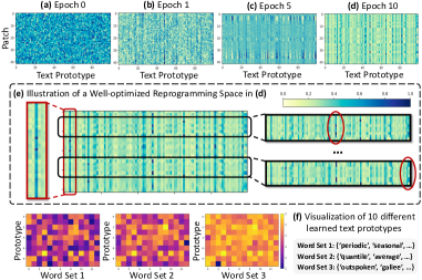
Figure 5: A showcase of patch reprogramming.

Reprogramming Interpretation. We provide a case study on ETTh1 of reprogramming 48 time series patches with 100 text prototypes in Figure 5. The top 4 subplots visualize the optimization of reprogramming space from randomly-initialized (a) to well-optimized (d). We find only a small set of prototypes (columns) participated in reprogramming the input patches (rows) in subplot (e). Also, patches undergo different representations through varying combinations of prototypes. This indicates: (1) text prototypes learn to summarize language cues, and a select few are highly relevant for representing information in local time series patches, which we visualize by randomly selecting 10 in subplot (f). Our results suggest a high relevance to the words that describe time series properties (i.e., word sets 1 and 2); (2) patches usually have different underlying semantics, necessitating different prototypes to represent.

Reprogramming Efficiency. Table 7 provides an overall efficiency analysis of Time-LLM with and without the backbone LLM. Our proposed reprogramming network itself (D.3) is lightweight in activating the LLM’s ability for time series forecasting (i.e., fewer than 6.6 million trainable parameters; only around 0.2% of the total parameters in Llama-7B), and the overall efficiency of Time-LLM is actually capped by the leveraged backbones (e.g., D.1 and D.2). This is favorable even compared to the parameter-efficient fine-tuning methods (e.g., QLoRA (Dettmers et al., 2023)) in balancing task performance and efficiency.

Table 7: Efficiency analysis of Time-LLM on ETTh1 in forecasting different steps ahead.

Length	ETTh1-96			ETTh1-192			ETTh1-336			ETTh1-512
Metric	Param. (M)	Mem. (MiB)	Speed(s/iter)	Param. (M)	Mem. (MiB)	Speed(s/iter)	Param. (M)	Mem. (MiB)	Speed(s/iter)	Param. (M)	Mem.(MiB)	Speed(s/iter)
D.1 LLama (32)	3404.53	32136	0.517	3404.57	33762	0.582	3404.62	37988	0.632	3404.69	39004	0.697
D.2 LLama (8)	975.83	11370	0.184	975.87	12392	0.192	975.92	13188	0.203	976.11	13616	0.217
D.3 w/o LLM	6.39	3678	0.046	6.42	3812	0.087	6.48	3960	0.093	6.55	4176	0.129

5 Conclusion and Future Work

TIME-LLM shows promise in adapting frozen large language models for time series forecasting by reprogramming time series data into text prototypes more natural for LLMs and providing natural language guidance via Prompt-as-Prefix to augment reasoning. Evaluations demonstrate the adapted LLMs can outperform specialized expert models, indicating their potential as effective time series machines. Our results also provide a novel insight that time series forecasting can be cast as yet another “language” task that can be tackled by an off-the-shelf LLM to achieve state-of-the-art performance through our Time-LLM framework. Further research should explore optimal reprogramming representations, enrich LLMs with explicit time series knowledge through continued pre-training, and build towards multimodal models with joint reasoning across time series, natural language, and other modalities. Furthermore, applying the reprogramming framework to equip LLMs with broader time series analytical abilities or other new capabilities should also be considered.

Appendix A More Related Work

Task-specific Learning. We furnish an extension of the related work on task-specific learning, focusing particularly on the most related models to which we made comparisons. Recent works improve Transformer (Vaswani et al., 2017) for time series forecasting by incorporating signal processing principles like patching, exponential smoothing, decomposition, and frequency analysis. For example, PatchTST (Nie et al., 2023) segments time series into patches as input tokens to Transformer. This retains local semantics, reduces computation/memory for attention, and allows longer history. It improves long-term forecast accuracy over other Transformer models. It also achieves excellent performance on self-supervised pretraining and transfer learning. ETSformer (Woo et al., 2022) incorporates exponential smoothing principles into Transformer attention to improve accuracy and efficiency. It uses exponential smoothing attention and frequency attention to replace standard self-attention. FEDformer (Zhou et al., 2022) combines Transformer with seasonal-trend decomposition. The decomposition captures the global profile while Transformer captures detailed structures. It also uses frequency enhancement for long-term prediction. This provides better performance and efficiency than the standard Transformer. Autoformer (Wu et al., 2021) uses a decomposition architecture with auto-correlation to enable progressive decomposition capacities for complex series. Auto-correlation is designed based on series periodicity to conduct dependency discovery and representation aggregation. It outperforms self-attention in efficiency and accuracy.

Although these methods enhance efficiency and accuracy compared to vanilla Transformer, they are mostly designed and optimized for narrow prediction tasks within specific domains. These models are typically trained end-to-end on small, domain-specific datasets. While achieving strong performance on their target tasks, such specialized models sacrifice versatility and generalizability across the diverse range of time series data encountered in the real world. The narrow focus limits their applicability to new datasets and tasks. To advance time series forecasting, there is a need for more flexible, widely applicable models that can adapt to new data distributions and tasks without extensive retraining. Ideal models would learn robust time series representations that transfer knowledge across domains. Developing such broadly capable forecasting models remains an open challenge. According to our discussions of related previous work, recent studies have begun to explore model versatility through pre-training and architectural innovations. However, further efforts are needed to realize the truly general-purpose forecasting systems that we are advancing in this research.

Cross-modality Adaptation. We provide an extended overview of related work in cross-modality adaptation, with a particular focus on recent advancements in model reprogramming for time series and other data modalities. Model reprogramming is a resource-efficient cross-domain learning approach that involves adapting a well-developed, pre-trained model from one domain (source) to address tasks in a different domain (target) without the need for model fine-tuning, even when these domains are significantly distinct, as noted by Chen (2022). In the context of time series data, Voice2Series (Yang et al., 2021) adapts an acoustic model from speech recognition for time series classification by transforming the time series to fit the model and remapping outputs to new labels. Similarly, LLMTime (Gruver et al., 2023) adapts LLMs for zero-shot time series forecasting, focusing on the effective tokenization of input time series for the backbone LLM, which then generates forecasts autoregressively. Diverging from these methods, Time-LLM does not edit the input time series directly. Instead, it proposes reprogramming time series with the source data modality along with prompting to unleash the full potential of LLMs as versatile forecasters in standard, few-shot, and zero-shot scenarios. Other notable works in this field, mostly in biology, include R2DL (Vinod et al., 2020) and ReproBert (Melnyk et al., 2023), which reprogram amino acids using word embeddings. A key distinction with our patch reprogramming approach is that, unlike the complete set of amino acids, time series patches do not form a complete set. Thus, we propose optimizing a small set of text prototypes and their mapping to time series patches, rather than directly optimizing a large transformation matrix between two complete sets, such as vocabulary and amino acids.

Appendix B Experimental Details

B.1 Implementation

We mainly follow the experimental configurations in (Wu et al., 2023) across all baselines within a unified evaluation pipeline in https://github.com/thuml/Time-Series-Library for fair comparisons. We use Llama-7B (Touvron et al., 2023) as the default backbone model unless stated otherwise. All our experiments are repeated three times and we report the averaged results. Our model implementation is on PyTorch (Paszke et al., 2019) with all experiments conducted on NVIDIA A100-80G GPUs. Our detailed model configurations are in Appendix B.4, and our code is made available at https://github.com/KimMeen/Time-LLM.

Technical Details. We provide additional technical details of Time-LLM in three aspects: (1) the learning of text prototypes, (2) the calculation of trends and lags in time series for use in prompts, and (3) the implementation of the output projection. To identify a small set of text prototypes $\mathbf{E^{\prime}}\in\mathbb{R}^{V^{\prime}\times D}$ from $\mathbf{E}\in\mathbb{R}^{V\times D}$, we learn a matrix $\mathbf{W}\in\mathbb{R}^{V^{\prime}\times V}$ as the intermediary. To describe the overall time series trend in natural language, we calculate the sum of differences between consecutive time steps. A sum greater than 0 indicates an upward trend, while a lesser sum denotes a downward trend. In addition, we calculate the top-5 lags of the time series, identified by computing the autocorrelation using fast Fourier transformation and selecting the five lags with the highest correlation values. After we pack and feedforward the prompt and patch embeddings $\mathbf{O}^{(i)}\in\mathbb{R}^{P\times D}$ through the frozen LLM, we discard the prefixal part and obtain the output representations, denoted as $\tilde{\mathbf{O}}^{i}\in\mathbb{R}^{P\times D}$. Subsequently, we follow PatchTST (Nie et al., 2023) and flatten $\tilde{\mathbf{O}}^{i}$ into a 1D tensor with the length $P\times D$, which is then linear projected as $\hat{\mathbf{Y}}^{i}\in\mathbb{R}^{H}$.

B.2 Dataset Details

Dataset statistics are summarized in Table 8. We evaluate the long-term forecasting performance on the well-established eight different benchmarks, including four ETT datasets (Zhou et al., 2021) (i.e., ETTh1, ETTh2, ETTm1, and ETTm2), Weather, Electricity, Traffic, and ILI from (Wu et al., 2023). Furthermore, we evaluate the performance of short-term forecasting on the M4 benchmark (Makridakis et al., 2018) and the quarterly dataset in the M3 benchmark (Makridakis & Hibon, 2000).

Table 8: Dataset statistics are from (Wu et al., 2023). The dimension indicates the number of time series (i.e., channels), and the dataset size is organized in (training, validation, testing).

Tasks	Dataset	Dim.	Series Length	Dataset Size	Frequency	Domain
	ETTm1	7	{96, 192, 336, 720}	(34465, 11521, 11521)	15 min	Temperature
Long-term	ETTm2	7	{96, 192, 336, 720}	(34465, 11521, 11521)	15 min	Temperature
Forecasting	ETTh1	7	{96, 192, 336, 720}	(8545, 2881, 2881)	1 hour	Temperature
	ETTh2	7	{96, 192, 336, 720}	(8545, 2881, 2881)	1 hour	Temperature
	Electricity	321	{96, 192, 336, 720}	(18317, 2633, 5261)	1 hour	Electricity
	Traffic	862	{96, 192, 336, 720}	(12185, 1757, 3509)	1 hour	Transportation
	Weather	21	{96, 192, 336, 720}	(36792, 5271, 10540)	10 min	Weather
	ILI	7	{24, 36, 48, 60}	(617, 74, 170)	1 week	Illness
	M3-Quarterly	1	8	(756, 0, 756)	Quarterly	Multiple
	M4-Yearly	1	6	(23000, 0, 23000)	Yearly	Demographic
	M4-Quarterly	1	8	(24000, 0, 24000)	Quarterly	Finance
Short-term	M4-Monthly	1	18	(48000, 0, 48000)	Monthly	Industry
Forecasting	M4-Weakly	1	13	(359, 0, 359)	Weakly	Macro
	M4-Daily	1	14	(4227, 0, 4227)	Daily	Micro
	M4-Hourly	1	48	(414, 0, 414)	Hourly	Other

The Electricity Transformer Temperature (ETT; An indicator reflective of long-term electric power deployment) benchmark is comprised of two years of data, sourced from two counties in China, and is subdivided into four distinct datasets, each with varying sampling rates: ETTh1 and ETTh2, which are sampled at a 1-hour level, and ETTm1 and ETTm2, which are sampled at a 15-minute level. Each entry within the ETT datasets includes six power load features and a target variable, termed “oil temperature”. The Electricity dataset comprises records of electricity consumption from 321 customers, measured at a 1-hour sampling rate. The Weather dataset includes one-year records from 21 meteorological stations located in Germany, with a sampling rate of 10 minutes. The Traffic dataset includes data on the occupancy rates of the freeway system, recorded from 862 sensors across the State of California, with a sampling rate of 1 hour. The influenza-like illness (ILI) dataset contains records of patients experiencing severe influenza with complications.

The M4 benchmark comprises 100K time series, amassed from various domains commonly present in business, financial, and economic forecasting. These time series have been partitioned into six distinctive datasets, each with varying sampling frequencies that range from yearly to hourly. The M3-Quarterly dataset comprises 756 quarterly sampled time series in the M3 benchmark. These series are categorized into five different domains: demographic, micro, macro, industry, and finance.

B.3 Evaluation Metrics

For evaluation metrics, we utilize the mean square error (MSE) and mean absolute error (MAE) for long-term forecasting. In terms of the short-term forecasting on M4 benchmark, we adopt the symmetric mean absolute percentage error (SMAPE), mean absolute scaled error (MASE), and overall weighted average (OWA) as in N-BEATS (Oreshkin et al., 2020). Note that OWA is a specific metric utilized in the M4 competition. The calculations of these metrics are as follows:

MSE $$=\frac{1}{H}\sum_{h=1}^{T}(\mathbf{Y}_{h}-\hat{\mathbf{Y}}_{h})^{2}, =\frac{1}{H}\sum_{h=1}^{H}|\mathbf{Y}_{h}-\hat{\mathbf{Y}}_{h}|,$$ MAE

SMAPE $$=\frac{200}{H}\sum_{h=1}^{H}\frac{|\mathbf{Y}_{h}-\hat{\mathbf{Y}}_{h}|}{|\mathbf{Y}_{h}|+|\hat{\mathbf{Y}}_{h}|}, =\frac{100}{H}\sum_{h=1}^{H}\frac{|\mathbf{Y}_{h}-\hat{\mathbf{Y}}_{h}|}{|\mathbf{Y}_{h}|},$$ MAPE

MASE $$=\frac{1}{H}\sum_{h=1}^{H}\frac{|\mathbf{Y}_{h}-\hat{\mathbf{Y}}_{h}|}{\frac{1}{H-s}\sum_{j=s+1}^{H}|\mathbf{Y}_{j}-\mathbf{Y}_{j-s}|}, =\frac{1}{2}\left[\frac{\text{SMAPE}}{\text{SMAPE}_{\textrm{Naïve2}}}+\frac{\text{MASE}}{\text{MASE}_{\textrm{Naïve2}}}\right],$$ OWA

where $s$ is the periodicity of the time series data. $H$ denotes the number of data points (i.e., prediction horizon in our cases). $\mathbf{Y}_{h}$ and $\hat{\mathbf{Y}}_{h}$ are the $h$-th ground truth and prediction where $h\in\{1,\cdots,H\}$.

B.4 Model Configurations

The configurations of our models, relative to varied tasks and datasets, are consolidated in Table 9. By default, the Adam optimizer (Kingma & Ba, 2015) is employed throughout all experiments. Specifically, the quantity of text prototypes $V^{\prime}$ is held constant at 100 and 1000 for short-term and long-term forecasting tasks, respectively. We utilize the Llama-7B model at full capacity, maintaining the backbone model layers at 32 across all tasks as a standard. The term input length $T$ signifies the number of time steps present in the original input time series data. Patch dimensions $d_{m}$ represent the hidden dimensions of the embedded time series patches prior to reprogramming. Lastly, heads $K$ correlate to the multi-head cross-attention utilized for patch reprogramming. In the four rightmost columns of Table 9, we detail the configurations related to model training.

Table 9: An overview of the experimental configurations for Time-LLM. “LTF” and “STF” denote long-term and short-term forecasting, respectively.

Task-Dataset / Configuration	Model Hyperparameter					Training Process
	Text Prototype $V^{\prime}$	Backbone Layers	Input Length $T$	Patch Dim. $d_{\text{m}}$	Heads $K$	LR∗	Loss	Batch Size	Epochs
LTF - ETTh1	1000	32	512	16	8	$10^{-3}$	MSE	16	50
LTF - ETTh2	1000	32	512	16	8	$10^{-3}$	MSE	16	50
LTF - ETTm1	1000	32	512	16	8	$10^{-3}$	MSE	16	100
LTF - ETTm2	1000	32	512	16	8	$10^{-3}$	MSE	16	100
LTF - Weather	1000	32	512	16	8	$10^{-2}$	MSE	8	100
LTF - Electricity	1000	32	512	16	8	$10^{-2}$	MSE	8	100
LTF - Traffic	1000	32	512	16	8	$10^{-2}$	MSE	8	100
LTF - ILI	100	32	96	16	8	$10^{-2}$	MSE	16	50
STF - M3-Quarterly	100	32	$2\times H$ †	32	8	$10^{-4}$	SMAPE	32	50
STF - M4	100	32	$2\times H$ †	32	8	$10^{-4}$	SMAPE	32	50

• ${\dagger}$ $H$ represents the forecasting horizon of the M4 and M3 datasets.

• $\ast$ LR means the initial learning rate.

Appendix C Hyperparameter Sensitivity

We conduct a hyperparameter sensitivity analysis focusing on the four important hyperparameters within Time-LLM: namely, the number of backbone model layers, the number of text prototypes $V^{\prime}$, the time series input length $T$, and the number of patch reprogramming cross-attention heads $K$. The correlated results can be found in Figure 6. From our analysis, we derive the following observations: (1) There is a positive correlation between the number of Transformer layers in the backbone LLM and the performance of Time-LLM, affirming that the scaling law is preserved post-LLM reprogramming.; (2) Generally, acquiring more text prototypes enhances performance. We hypothesize that a limited number of prototypes $V^{\prime}$ might induce noise when aggregating language cues, consequently obstructing the efficient learning of highly representative prototypes essential for characterizing the input time series patches; (3) The input time length $T$ exhibits a direct relation with forecasting accuracy, particularly evident when predicting extended horizons. This observation is logical and is in congruence with conventional time series models; (4) Increasing the number of attention heads during the reprogramming of input patches proves to be advantageous.

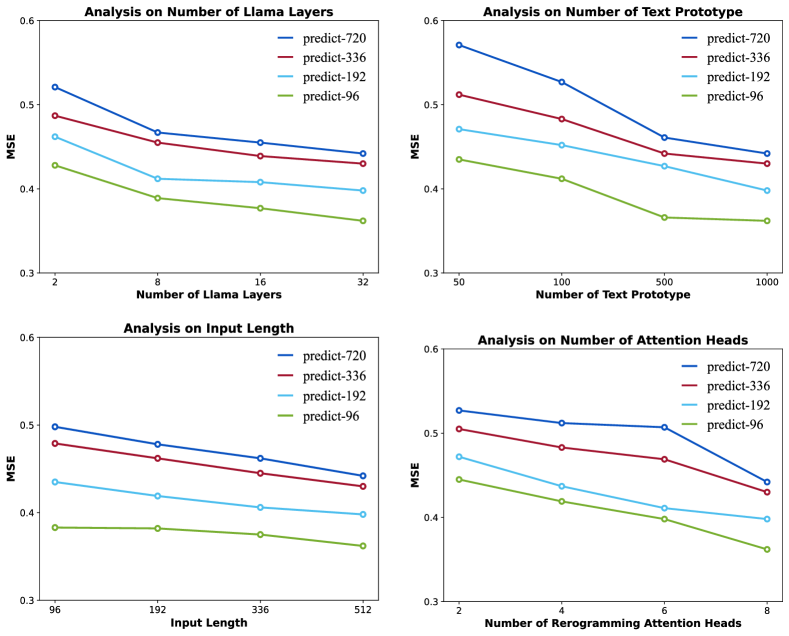
Figure 6: Analysis of hyperparameter sensitivity on ETTh1 dataset.

Appendix D Long-term and Short-term Forecasting

D.1 Long-term Forecasting

By solely reprogramming the smallest Llama model while keeping it intact, Time-LLM attains SOTA performance in 36 out of 40 instances across eight time series benchmarks. This underscores the considerable potential of LLMs as robust and reliable time series forecasters. Furthermore, we benchmark the proposed method against other well-established baselines in Table 11. This comparison includes three notable statistical methods (AutoARIMA, AutoTheta, and AutoETS) (Herzen et al., 2022) and two recent time series models, N-HiTS (Challu et al., 2023b) and N-BEATS (Oreshkin et al., 2020). Remarkably, Time-LLM secures SOTA performance across all cases, surpassing the second-best results by significant margins of over 22% and 16% in terms of MSE and MAE.

Table 10: Full long-term forecasting results. We set the forecasting horizons $H\in\{24,36,48,60\}$ for ILI and $\{96,192,336,720\}$ for the others. A lower value indicates better performance. Red: the best, Blue: the second best.

Methods		Time-LLM		GPT4TS		DLinear		PatchTST		TimesNet		FEDformer		Autoformer		Stationary		ETSformer		LightTS		Informer		Reformer
Metric		MSE	MAE	MSE	MAE	MSE	MAE	MSE	MAE	MSE	MAE	MSE	MAE	MSE	MAE	MSE	MAE	MSE	MAE	MSE	MAE	MSE	MAE	MSE	MAE
$ETTh1$	96	0.362	0.392	0.376	0.397	0.375	0.399	0.370	0.399	0.384	0.402	0.376	0.419	0.449	0.459	0.513	0.491	0.494	0.479	0.424	0.432	0.865	0.713	0.837	0.728
	192	0.398	0.418	0.416	0.418	0.405	0.416	0.413	0.421	0.436	0.429	0.420	0.448	0.500	0.482	0.534	0.504	0.538	0.504	0.475	0.462	1.008	0.792	0.923	0.766
	336	0.430	0.427	0.442	0.433	0.439	0.443	0.422	0.436	0.491	0.469	0.459	0.465	0.521	0.496	0.588	0.535	0.574	0.521	0.518	0.488	1.107	0.809	1.097	0.835
	720	0.442	0.457	0.477	0.456	0.472	0.490	0.447	0.466	0.521	0.500	0.506	0.507	0.514	0.512	0.643	0.616	0.562	0.535	0.547	0.533	1.181	0.865	1.257	0.889
	Avg	0.408	0.423	0.465	0.455	0.422	0.437	0.413	0.430	0.458	0.450	0.440	0.460	0.496	0.487	0.570	0.537	0.542	0.510	0.491	0.479	1.040	0.795	1.029	0.805
$ETTh2$	96	0.268	0.328	0.285	0.342	0.289	0.353	0.274	0.336	0.340	0.374	0.358	0.397	0.346	0.388	0.476	0.458	0.340	0.391	0.397	0.437	3.755	1.525	2.626	1.317
	192	0.329	0.375	0.354	0.389	0.383	0.418	0.339	0.379	0.402	0.414	0.429	0.439	0.456	0.452	0.512	0.493	0.430	0.439	0.520	0.504	5.602	1.931	11.12	2.979
	336	0.368	0.409	0.373	0.407	0.448	0.465	0.329	0.380	0.452	0.452	0.496	0.487	0.482	0.486	0.552	0.551	0.485	0.479	0.626	0.559	4.721	1.835	9.323	2.769
	720	0.372	0.420	0.406	0.441	0.605	0.551	0.379	0.422	0.462	0.468	0.463	0.474	0.515	0.511	0.562	0.560	0.500	0.497	0.863	0.672	3.647	1.625	3.874	1.697
	Avg	0.334	0.383	0.381	0.412	0.431	0.446	0.330	0.379	0.414	0.427	0.437	0.449	0.450	0.459	0.526	0.516	0.439	0.452	0.602	0.543	4.431	1.729	6.736	2.191
$ETTm1$	96	0.272	0.334	0.292	0.346	0.299	0.343	0.290	0.342	0.338	0.375	0.379	0.419	0.505	0.475	0.386	0.398	0.375	0.398	0.374	0.400	0.672	0.571	0.538	0.528
	192	0.310	0.358	0.332	0.372	0.335	0.365	0.332	0.369	0.374	0.387	0.426	0.441	0.553	0.496	0.459	0.444	0.408	0.410	0.400	0.407	0.795	0.669	0.658	0.592
	336	0.352	0.384	0.366	0.394	0.369	0.386	0.366	0.392	0.410	0.411	0.445	0.459	0.621	0.537	0.495	0.464	0.435	0.428	0.438	0.438	1.212	0.871	0.898	0.721
	720	0.383	0.411	0.417	0.421	0.425	0.421	0.416	0.420	0.478	0.450	0.543	0.490	0.671	0.561	0.585	0.516	0.499	0.462	0.527	0.502	1.166	0.823	1.102	0.841
	Avg	0.329	0.372	0.388	0.403	0.357	0.378	0.351	0.380	0.400	0.406	0.448	0.452	0.588	0.517	0.481	0.456	0.429	0.425	0.435	0.437	0.961	0.734	0.799	0.671
$ETTm2$	96	0.161	0.253	0.173	0.262	0.167	0.269	0.165	0.255	0.187	0.267	0.203	0.287	0.255	0.339	0.192	0.274	0.189	0.280	0.209	0.308	0.365	0.453	0.658	0.619
	192	0.219	0.293	0.229	0.301	0.224	0.303	0.220	0.292	0.249	0.309	0.269	0.328	0.281	0.340	0.280	0.339	0.253	0.319	0.311	0.382	0.533	0.563	1.078	0.827
	336	0.271	0.329	0.286	0.341	0.281	0.342	0.274	0.329	0.321	0.351	0.325	0.366	0.339	0.372	0.334	0.361	0.314	0.357	0.442	0.466	1.363	0.887	1.549	0.972
	720	0.352	0.379	0.378	0.401	0.397	0.421	0.362	0.385	0.408	0.403	0.421	0.415	0.433	0.432	0.417	0.413	0.414	0.413	0.675	0.587	3.379	1.338	2.631	1.242
	Avg	0.251	0.313	0.284	0.339	0.267	0.333	0.255	0.315	0.291	0.333	0.305	0.349	0.327	0.371	0.306	0.347	0.293	0.342	0.409	0.436	1.410	0.810	1.479	0.915
${{\color[rgb]{0,0,0}Weather}}$	96	0.147	0.201	0.162	0.212	0.176	0.237	0.149	0.198	0.172	0.220	0.217	0.296	0.266	0.336	0.173	0.223	0.197	0.281	0.182	0.242	0.300	0.384	0.689	0.596
	192	0.189	0.234	0.204	0.248	0.220	0.282	0.194	0.241	0.219	0.261	0.276	0.336	0.307	0.367	0.245	0.285	0.237	0.312	0.227	0.287	0.598	0.544	0.752	0.638
	336	0.262	0.279	0.254	0.286	0.265	0.319	0.245	0.282	0.280	0.306	0.339	0.380	0.359	0.395	0.321	0.338	0.298	0.353	0.282	0.334	0.578	0.523	0.639	0.596
	720	0.304	0.316	0.326	0.337	0.333	0.362	0.314	0.334	0.365	0.359	0.403	0.428	0.419	0.428	0.414	0.410	0.352	0.288	0.352	0.386	1.059	0.741	1.130	0.792
	Avg	0.225	0.257	0.237	0.270	0.248	0.300	0.225	0.264	0.259	0.287	0.309	0.360	0.338	0.382	0.288	0.314	0.271	0.334	0.261	0.312	0.634	0.548	0.803	0.656
${{\color[rgb]{0,0,0}Electricity}}$	96	0.131	0.224	0.139	0.238	0.140	0.237	0.129	0.222	0.168	0.272	0.193	0.308	0.201	0.317	0.169	0.273	0.187	0.304	0.207	0.307	0.274	0.368	0.312	0.402
	192	0.152	0.241	0.153	0.251	0.153	0.249	0.157	0.240	0.184	0.289	0.201	0.315	0.222	0.334	0.182	0.286	0.199	0.315	0.213	0.316	0.296	0.386	0.348	0.433
	336	0.160	0.248	0.169	0.266	0.169	0.267	0.163	0.259	0.198	0.300	0.214	0.329	0.231	0.338	0.200	0.304	0.212	0.329	0.230	0.333	0.300	0.394	0.350	0.433
	720	0.192	0.298	0.206	0.297	0.203	0.301	0.197	0.290	0.220	0.320	0.246	0.355	0.254	0.361	0.222	0.321	0.233	0.345	0.265	0.360	0.373	0.439	0.340	0.420
	Avg	0.158	0.252	0.167	0.263	0.166	0.263	0.161	0.252	0.192	0.295	0.214	0.327	0.227	0.338	0.193	0.296	0.208	0.323	0.229	0.329	0.311	0.397	0.338	0.422
${{\color[rgb]{0,0,0}Traffic}}$	96	0.362	0.248	0.388	0.282	0.410	0.282	0.360	0.249	0.593	0.321	0.587	0.366	0.613	0.388	0.612	0.338	0.607	0.392	0.615	0.391	0.719	0.391	0.732	0.423
	192	0.374	0.247	0.407	0.290	0.423	0.287	0.379	0.256	0.617	0.336	0.604	0.373	0.616	0.382	0.613	0.340	0.621	0.399	0.601	0.382	0.696	0.379	0.733	0.420
	336	0.385	0.271	0.412	0.294	0.436	0.296	0.392	0.264	0.629	0.336	0.621	0.383	0.622	0.337	0.618	0.328	0.622	0.396	0.613	0.386	0.777	0.420	0.742	0.420
	720	0.430	0.288	0.450	0.312	0.466	0.315	0.432	0.286	0.640	0.350	0.626	0.382	0.660	0.408	0.653	0.355	0.632	0.396	0.658	0.407	0.864	0.472	0.755	0.423
	Avg	0.388	0.264	0.414	0.294	0.433	0.295	0.390	0.263	0.620	0.336	0.610	0.376	0.628	0.379	0.624	0.340	0.621	0.396	0.622	0.392	0.764	0.416	0.741	0.422
${{\color[rgb]{0,0,0}ILI}}$	24	1.285	0.727	2.063	0.881	2.215	1.081	1.319	0.754	2.317	0.934	3.228	1.260	3.483	1.287	2.294	0.945	2.527	1.020	8.313	2.144	5.764	1.677	4.400	1.382
	36	1.404	0.814	1.868	0.892	1.963	0.963	1.430	0.834	1.972	0.920	2.679	1.080	3.103	1.148	1.825	0.848	2.615	1.007	6.631	1.902	4.755	1.467	4.783	1.448
	48	1.523	0.807	1.790	0.884	2.130	1.024	1.553	0.815	2.238	0.940	2.622	1.078	2.669	1.085	2.010	0.900	2.359	0.972	7.299	1.982	4.763	1.469	4.832	1.465
	60	1.531	0.854	1.979	0.957	2.368	1.096	1.470	0.788	2.027	0.928	2.857	1.157	2.770	1.125	2.178	0.963	2.487	1.016	7.283	1.985	5.264	1.564	4.882	1.483
	Avg	1.435	0.801	1.925	0.903	2.169	1.041	1.443	0.797	2.139	0.931	2.847	1.144	3.006	1.161	2.077	0.914	2.497	1.004	7.382	2.003	5.137	1.544	4.724	1.445
$1^{\text{st}}$Count		36		0		1		17		0		0		0		0		0		0		0		0

Table 11: Additional comparison with other baselines in long-term forecasting tasks. We set the forecasting horizons $H\in\{24,36,48,60\}$ for ILI and $\{96,192,336,720\}$ for the others. A lower value indicates better performance. Red: the best, Blue: the second best.

Methods		Time-LLM		N-BEATS		N-HiTS		AutoARIMA		AutoTheta		AutoETS
Metric		MSE	MAE	MSE	MAE	MSE	MAE	MSE	MAE	MSE	MAE	MSE	MAE
$ETTh1$	96	0.362	0.392	0.496	0.475	0.392	0.407	0.933	0.635	1.266	0.758	1.264	0.756
	192	0.398	0.418	0.544	0.504	0.442	0.438	0.868	0.621	1.188	0.749	1.181	0.745
	336	0.430	0.427	0.592	0.533	0.497	0.471	0.964	0.663	1.310	0.799	1.292	0.792
	720	0.442	0.457	0.639	0.588	0.559	0.533	1.043	0.705	1.510	0.882	1.405	0.842
	Avg	0.408	0.423	0.568	0.525	0.473	0.462	0.952	0.656	1.319	0.797	1.286	0.784
$ETTh2$	96	0.268	0.328	0.384	0.431	0.321	0.368	0.390	0.417	0.461	0.430	0.444	0.403
	192	0.329	0.375	0.496	0.493	0.398	0.421	0.545	0.492	0.754	0.537	0.771	0.461
	336	0.368	0.409	0.585	0.542	0.453	0.459	0.697	0.562	1.355	0.683	1.526	0.522
	720	0.372	0.420	0.792	0.651	0.775	0.609	0.907	0.658	3.971	1.061	5.183	0.633
	Avg	0.334	0.383	0.564	0.529	0.487	0.464	0.635	0.532	1.635	0.678	1.981	0.505
$ETTm1$	96	0.272	0.334	0.393	0.412	0.327	0.368	1.091	0.661	1.211	0.704	1.519	0.768
	192	0.310	0.358	0.425	0.427	0.376	0.400	1.119	0.682	1.237	0.724	1.535	0.784
	336	0.352	0.384	0.464	0.454	0.407	0.423	1.125	0.698	1.231	0.735	1.472	0.782
	720	0.383	0.411	0.521	0.488	0.471	0.456	1.243	0.745	1.394	0.801	1.591	0.825
	Avg	0.329	0.372	0.451	0.445	0.395	0.412	1.145	0.697	1.268	0.741	1.529	0.790
$ETTm2$	96	0.161	0.253	0.204	0.302	0.188	0.273	0.435	0.375	0.245	0.316	0.359	0.333
	192	0.219	0.293	0.282	0.358	0.274	0.338	0.995	0.494	0.413	0.401	0.756	0.396
	336	0.271	0.329	0.378	0.425	0.384	0.406	2.324	0.648	0.790	0.528	1.747	0.467
	720	0.352	0.379	0.555	0.523	0.501	0.488	9.064	1.020	2.451	0.847	6.856	0.639
	Avg	0.251	0.313	0.355	0.402	0.337	0.376	3.205	0.634	0.975	0.523	2.430	0.459
${{\color[rgb]{0,0,0}Weather}}$	96	0.147	0.201	0.185	0.244	0.160	0.222	0.255	0.273	0.279	0.266	0.331	0.277
	192	0.189	0.234	0.225	0.282	0.202	0.265	0.390	0.353	0.337	0.316	0.498	0.345
	336	0.262	0.279	0.274	0.323	0.253	0.303	0.775	0.457	0.472	0.385	0.898	0.423
	720	0.304	0.316	0.340	0.373	0.323	0.354	2.898	0.707	0.818	0.526	2.820	0.580
	Avg	0.225	0.257	0.256	0.306	0.235	0.286	1.080	0.448	0.477	0.373	1.137	0.406
${{\color[rgb]{0,0,0}Electricity}}$	96	0.131	0.224	0.233	0.327	0.184	0.275	0.520	0.466	0.653	0.532	0.650	0.526
	192	0.152	0.241	0.246	0.340	0.190	0.282	0.581	0.499	0.713	0.561	0.704	0.549
	336	0.160	0.248	0.262	0.355	0.205	0.298	0.602	0.515	0.797	0.603	0.766	0.577
	720	0.192	0.298	0.296	0.383	0.239	0.330	0.685	0.558	1.023	0.688	0.901	0.628
	Avg	0.158	0.252	0.259	0.351	0.205	0.296	0.597	0.510	0.797	0.596	0.755	0.570
${{\color[rgb]{0,0,0}Traffic}}$	96	0.362	0.248	0.608	0.447	0.410	0.329	1.068	0.694	3.207	1.219	3.254	1.221
	192	0.374	0.247	0.605	0.448	0.414	0.330	1.380	0.775	3.407	1.262	3.569	1.264
	336	0.385	0.271	0.618	0.454	0.428	0.337	1.448	0.790	3.473	1.274	3.971	1.275
	720	0.430	0.288	0.650	0.467	0.456	0.354	1.481	0.799	3.952	1.382	6.784	1.379
	Avg	0.388	0.264	0.620	0.454	0.427	0.338	1.344	0.765	3.510	1.284	4.395	1.285
${{\color[rgb]{0,0,0}ILI}}$	24	1.285	0.727	6.809	1.870	2.675	1.080	4.909	1.329	5.991	1.510	4.869	1.315
	36	1.404	0.814	6.850	1.890	3.081	1.194	5.079	1.440	5.922	1.539	4.917	1.422
	48	1.523	0.807	6.788	1.876	2.973	1.176	4.276	1.339	4.637	1.329	3.966	1.301
	60	1.531	0.854	6.908	1.893	3.259	1.232	3.855	1.276	4.378	1.345	3.540	1.229
	Avg	1.435	0.801	6.839	1.882	2.997	1.171	4.530	1.346	5.232	1.431	4.323	1.317
$1^{\text{st}}$Count		40		0		1		0		0		0

D.2 Short-term Forecasting

Table 12: Full short-term time series forecasting results. The forecasting horizons are in [6, 48] and the last three rows are weighted averaged from all datasets under different sampling intervals. A lower value indicates better performance. Red: the best, Blue: the second best.

Methods		Time-LLM	GPT4TS	TimesNet	PatchTST	N-HiTS	N-BEATS	ETSformer	LightTS	DLinear	FEDformer	Stationary	Autoformer	Informer	Reformer
Yearly	SMAPE	13.419	15.11	15.378	13.477	13.422	13.487	18.009	14.247	16.965	14.021	13.717	13.974	14.727	16.169
	MASE	3.005	3.565	3.554	3.019	3.056	3.036	4.487	3.109	4.283	3.036	3.078	3.134	3.418	3.800
	OWA	0.789	0.911	0.918	0.792	0.795	0.795	1.115	0.827	1.058	0.811	0.807	0.822	0.881	0.973
Quarterly	SMAPE	10.110	10.597	10.465	10.38	10.185	10.564	13.376	11.364	12.145	11.1	10.958	11.338	11.360	13.313
	MASE	1.178	1.253	1.227	1.233	1.18	1.252	1.906	1.328	1.520	1.35	1.325	1.365	1.401	1.775
	OWA	0.889	0.938	0.923	0.921	0.893	0.936	1.302	1.000	1.106	0.996	0.981	1.012	1.027	1.252
Monthly	SMAPE	12.980	13.258	13.513	12.959	13.059	13.089	14.588	14.014	13.514	14.403	13.917	13.958	14.062	20.128
	MASE	0.963	1.003	1.039	0.97	1.013	0.996	1.368	1.053	1.037	1.147	1.097	1.103	1.141	2.614
	OWA	0.903	0.931	0.957	0.905	0.929	0.922	1.149	0.981	0.956	1.038	0.998	1.002	1.024	1.927
Others	SMAPE	4.795	6.124	6.913	4.952	4.711	6.599	7.267	15.880	6.709	7.148	6.302	5.485	24.460	32.491
	MASE	3.178	4.116	4.507	3.347	3.054	4.43	5.240	11.434	4.953	4.041	4.064	3.865	20.960	33.355
	OWA	1.006	1.259	1.438	1.049	0.977	1.393	1.591	3.474	1.487	1.389	1.304	1.187	5.879	8.679
Average	SMAPE	11.983	12.69	12.88	12.059	12.035	12.25	14.718	13.525	13.639	13.16	12.780	12.909	14.086	18.200
	MASE	1.595	1.808	1.836	1.623	1.625	1.698	2.408	2.111	2.095	1.775	1.756	1.771	2.718	4.223
	OWA	0.859	0.94	0.955	0.869	0.869	0.896	1.172	1.051	1.051	0.949	0.930	0.939	1.230	1.775

Table 13: Additional short-term time series forecasting results on M3 (Quarterly). The forecasting horizon is 8. A lower value indicates better performance. Red: the best, Blue: the second best.

Methods		Time-LLM	GPT4TS	TimesNet	PatchTST	N-HiTS	N-BEATS	DLinear	FEDformer
	SMAPE	11.171	14.453	10.410	12.380	12.616	18.640	15.028	12.927
	MRAE	3.282	5.035	3.310	2.401	4.271	4.612	2.793	3.653
	MAPE	0.151	0.203	0.140	0.154	0.168	0.247	0.196	0.174

Our complete results on short-term forecasting are presented in Table 12. Time-LLM consistently outperforms the majority of baseline models in most cases. Notably, we surpass GPT4TS by a large margin (e.g., 8.7% overall, 13.4% on M4-Yearly, and an average of 21.5% on M4-Hourly, M4-Daily, and M4-Weekly), as well as TimesNet (e.g., 10% overall, 14.1% on M4-Yearly, and an average of 30.1% on M4-Hourly, M4-Daily, and M4-Weekly). Compared to the recent state-of-the-art forecasting models, N-HiTS and PatchTST, Time-LLM exhibits comparable or superior performances without any parameter updates on the backbone LLM.

In addition, we conduct a comparative analysis between Time-LLM and the top-performing models on the M3-Quarterly dataset, with the findings presented in Table 13. We provide additional metrics, namely MRAE and MAPE, alongside the default SMAPE used in the M3 competition. On this dataset, Time-LLM attains on-par performance compared to TimesNet and PatchTST, outperforming GPT4TS by substantial margins, achieving reductions of over 23%, 35%, and 26% in SMAPE, MRAE, and MAPE, respectively.

Appendix E Few-shot and Zero-shot Forecasting

E.1 Few-shot Forecasting

Table 14: Full few-shot learning results on 10% training data. We use the same protocol as in Table 1.

Methods		Time-LLM		GPT4TS		DLinear		PatchTST		TimesNet		FEDformer		Autoformer		Stationary		ETSformer		LightTS		Informer		Reformer
Metric		MSE	MAE	MSE	MAE	MSE	MAE	MSE	MAE	MSE	MAE	MSE	MAE	MSE	MAE	MSE	MAE	MSE	MAE	MSE	MAE	MSE	MAE	MSE	MAE
$ETTh1$	96	0.448	0.460	0.458	0.456	0.492	0.495	0.516	0.485	0.861	0.628	0.512	0.499	0.613	0.552	0.918	0.639	1.112	0.806	1.298	0.838	1.179	0.792	1.184	0.790
	192	0.484	0.483	0.570	0.516	0.565	0.538	0.598	0.524	0.797	0.593	0.624	0.555	0.722	0.598	0.915	0.629	1.155	0.823	1.322	0.854	1.199	0.806	1.295	0.850
	336	0.589	0.540	0.608	0.535	0.721	0.622	0.657	0.550	0.941	0.648	0.691	0.574	0.750	0.619	0.939	0.644	1.179	0.832	1.347	0.870	1.202	0.811	1.294	0.854
	720	0.700	0.604	0.725	0.591	0.986	0.743	0.762	0.610	0.877	0.641	0.728	0.614	0.721	0.616	0.887	0.645	1.273	0.874	1.534	0.947	1.217	0.825	1.223	0.838
	Avg	0.556	0.522	0.590	0.525	0.691	0.600	0.633	0.542	0.869	0.628	0.639	0.561	0.702	0.596	0.915	0.639	1.180	0.834	1.375	0.877	1.199	0.809	1.249	0.833
$ETTh2$	96	0.275	0.326	0.331	0.374	0.357	0.411	0.353	0.389	0.378	0.409	0.382	0.416	0.413	0.451	0.389	0.411	0.678	0.619	2.022	1.006	3.837	1.508	3.788	1.533
	192	0.374	0.373	0.402	0.411	0.569	0.519	0.403	0.414	0.490	0.467	0.478	0.474	0.474	0.477	0.473	0.455	0.785	0.666	2.329	1.104	3.856	1.513	3.552	1.483
	336	0.406	0.429	0.406	0.433	0.671	0.572	0.426	0.441	0.537	0.494	0.504	0.501	0.547	0.543	0.507	0.480	0.839	0.694	2.453	1.122	3.952	1.526	3.395	1.526
	720	0.427	0.449	0.449	0.464	0.824	0.648	0.477	0.480	0.510	0.491	0.499	0.509	0.516	0.523	0.477	0.472	1.273	0.874	3.816	1.407	3.842	1.503	3.205	1.401
	Avg	0.370	0.394	0.397	0.421	0.605	0.538	0.415	0.431	0.479	0.465	0.466	0.475	0.488	0.499	0.462	0.455	0.894	0.713	2.655	1.160	3.872	1.513	3.485	1.486
$ETTm1$	96	0.346	0.388	0.390	0.404	0.352	0.392	0.410	0.419	0.583	0.501	0.578	0.518	0.774	0.614	0.761	0.568	0.911	0.688	0.921	0.682	1.162	0.785	1.442	0.847
	192	0.373	0.416	0.429	0.423	0.382	0.412	0.437	0.434	0.630	0.528	0.617	0.546	0.754	0.592	0.781	0.574	0.955	0.703	0.957	0.701	1.172	0.793	1.444	0.862
	336	0.413	0.426	0.469	0.439	0.419	0.434	0.476	0.454	0.725	0.568	0.998	0.775	0.869	0.677	0.803	0.587	0.991	0.719	0.998	0.716	1.227	0.908	1.450	0.866
	720	0.485	0.476	0.569	0.498	0.490	0.477	0.681	0.556	0.769	0.549	0.693	0.579	0.810	0.630	0.844	0.581	1.062	0.747	1.007	0.719	1.207	0.797	1.366	0.850
	Avg	0.404	0.427	0.464	0.441	0.411	0.429	0.501	0.466	0.677	0.537	0.722	0.605	0.802	0.628	0.797	0.578	0.980	0.714	0.971	0.705	1.192	0.821	1.426	0.856
$ETTm2$	96	0.177	0.261	0.188	0.269	0.213	0.303	0.191	0.274	0.212	0.285	0.291	0.399	0.352	0.454	0.229	0.308	0.331	0.430	0.813	0.688	3.203	1.407	4.195	1.628
	192	0.241	0.314	0.251	0.309	0.278	0.345	0.252	0.317	0.270	0.323	0.307	0.379	0.694	0.691	0.291	0.343	0.400	0.464	1.008	0.768	3.112	1.387	4.042	1.601
	336	0.274	0.327	0.307	0.346	0.338	0.385	0.306	0.353	0.323	0.353	0.543	0.559	2.408	1.407	0.348	0.376	0.469	0.498	1.031	0.775	3.255	1.421	3.963	1.585
	720	0.417	0.390	0.426	0.417	0.436	0.440	0.433	0.427	0.474	0.449	0.712	0.614	1.913	1.166	0.461	0.438	0.589	0.557	1.096	0.791	3.909	1.543	3.711	1.532
	Avg	0.277	0.323	0.293	0.335	0.316	0.368	0.296	0.343	0.320	0.353	0.463	0.488	1.342	0.930	0.332	0.366	0.447	0.487	0.987	0.756	3.370	1.440	3.978	1.587
${{\color[rgb]{0,0,0}Weather}}$	96	0.161	0.210	0.163	0.215	0.171	0.224	0.165	0.215	0.184	0.230	0.188	0.253	0.221	0.297	0.192	0.234	0.199	0.272	0.217	0.269	0.374	0.401	0.335	0.380
	192	0.204	0.248	0.210	0.254	0.215	0.263	0.210	0.257	0.245	0.283	0.250	0.304	0.270	0.322	0.269	0.295	0.279	0.332	0.259	0.304	0.552	0.478	0.522	0.462
	336	0.261	0.302	0.256	0.292	0.258	0.299	0.259	0.297	0.305	0.321	0.312	0.346	0.320	0.351	0.370	0.357	0.356	0.386	0.303	0.334	724	0.541	0.715	0.535
	720	0.309	0.332	0.321	0.339	0.320	0.346	0.332	0.346	0.381	0.371	0.387	0.393	0.390	0.396	0.441	0.405	0.437	0.448	0.377	0.382	0.739	0.558	0.611	0.500
	Avg	0.234	0.273	0.238	0.275	0.241	0.283	0.242	0.279	0.279	0.301	0.284	0.324	0.300	0.342	0.318	0.323	0.318	0.360	0.289	0.322	0.597	0.495	0.546	0.469
${{\color[rgb]{0,0,0}Electricity}}$	96	0.139	0.241	0.139	0.237	0.150	0.253	0.140	0.238	0.299	0.373	0.231	0.323	0.261	0.348	0.420	0.466	0.599	0.587	0.350	0.425	1.259	0.919	0.993	0.784
	192	0.151	0.248	0.156	0.252	0.164	0.264	0.160	0.255	0.305	0.379	0.261	0.356	0.338	0.406	0.411	0.459	0.620	0.598	0.376	0.448	1.160	0.873	0.938	0.753
	336	0.169	0.270	0.175	0.270	0.181	0.282	0.180	0.276	0.319	0.391	0.360	0.445	0.410	0.474	0.434	0.473	0.662	0.619	0.428	0.485	1.157	0.872	0.925	0.745
	720	0.240	0.322	0.233	0.317	0.223	0.321	0.241	0.323	0.369	0.426	0.530	0.585	0.715	0.685	0.510	0.521	0.757	0.664	0.611	0.597	1.203	0.898	1.004	0.790
	Avg	0.175	0.270	0.176	0.269	0.180	0.280	0.180	0.273	0.323	0.392	0.346	0.427	0.431	0.478	0.444	0.480	0.660	0.617	0.441	0.489	1.195	0.891	0.965	0.768
${{\color[rgb]{0,0,0}Traffic}}$	96	0.418	0.291	0.414	0.297	0.419	0.298	0.403	0.289	0.719	0.416	0.639	0.400	0.672	0.405	1.412	0.802	1.643	0.855	1.157	0.636	1.557	0.821	1.527	0.815
	192	0.414	0.296	0.426	0.301	0.434	0.305	0.415	0.296	0.748	0.428	0.637	0.416	0.727	0.424	1.419	0.806	1.641	0.854	1.207	0.661	1.454	0.765	1.538	0.817
	336	0.421	0.311	0.434	0.303	0.449	0.313	0.426	0.304	0.853	0.471	0.655	0.427	0.749	0.454	1.443	0.815	1.711	0.878	1.334	0.713	1.521	0.812	1.550	0.819
	720	0.462	0.327	0.487	0.337	0.484	0.336	0.474	0.331	1.485	0.825	0.722	0.456	0.847	0.499	1.539	0.837	2.660	1.157	1.292	0.726	1.605	0.846	1.588	0.833
	Avg	0.429	0.306	0.440	0.310	0.447	0.313	0.430	0.305	0.951	0.535	0.663	0.425	0.749	0.446	1.453	0.815	1.914	0.936	1.248	0.684	1.534	0.811	1.551	0.821
$1^{\text{st}}$Count		32		9		3		3		0		0		0		0		0		0		0		0

Table 15: Full few-shot learning results on 5% training data. We use the same protocol as in Table 1. ’-’ means that 5% time series is not sufficient to constitute a training set.

Methods		Time-LLM		GPT4TS		DLinear		PatchTST		TimesNet		FEDformer		Autoformer		Stationary		ETSformer		LightTS		Informer		Reformer
Metric		MSE	MAE	MSE	MAE	MSE	MAE	MSE	MAE	MSE	MAE	MSE	MAE	MSE	MAE	MSE	MAE	MSE	MAE	MSE	MAE	MSE	MAE	MSE	MAE
$ETTh1$	96	0.483	0.464	0.543	0.506	0.547	0.503	0.557	0.519	0.892	0.625	0.593	0.529	0.681	0.570	0.952	0.650	1.169	0.832	1.483	0.91	1.225	0.812	1.198	0.795
	192	0.629	0.540	0.748	0.580	0.720	0.604	0.711	0.570	0.940	0.665	0.652	0.563	0.725	0.602	0.943	0.645	1.221	0.853	1.525	0.93	1.249	0.828	1.273	0.853
	336	0.768	0.626	0.754	0.595	0.984	0.727	0.816	0.619	0.945	0.653	0.731	0.594	0.761	0.624	0.935	0.644	1.179	0.832	1.347	0.87	1.202	0.811	1.254	0.857
	720	-	-	-	-	-	-	-	-	-	-	-	-	-	-	-	-	-	-	-	-	-	-	-	-
	Avg	0.627	0.543	0.681	0.560	0.750	0.611	0.694	0.569	0.925	0.647	0.658	0.562	0.722	0.598	0.943	0.646	1.189	0.839	1.451	0.903	1.225	0.817	1.241	0.835
$ETTh2$	96	0.336	0.397	0.376	0.421	0.442	0.456	0.401	0.421	0.409	0.420	0.390	0.424	0.428	0.468	0.408	0.423	0.678	0.619	2.022	1.006	3.837	1.508	3.753	1.518
	192	0.406	0.425	0.418	0.441	0.617	0.542	0.452	0.455	0.483	0.464	0.457	0.465	0.496	0.504	0.497	0.468	0.845	0.697	3.534	1.348	3.975	1.933	3.516	1.473
	336	0.405	0.432	0.408	0.439	1.424	0.849	0.464	0.469	0.499	0.479	0.477	0.483	0.486	0.496	0.507	0.481	0.905	0.727	4.063	1.451	3.956	1.520	3.312	1.427
	720	-	-	-	-	-	-	-	-	-	-	-	-	-	-	-	-	-	-	-	-	-	-	-	-
	Avg	0.382	0.418	0.400	0.433	0.694	0.577	0.827	0.615	0.439	0.448	0.463	0.454	0.441	0.457	0.470	0.489	0.809	0.681	3.206	1.268	3.922	1.653	3.527	1.472
$ETTm1$	96	0.316	0.377	0.386	0.405	0.332	0.374	0.399	0.414	0.606	0.518	0.628	0.544	0.726	0.578	0.823	0.587	1.031	0.747	1.048	0.733	1.130	0.775	1.234	0.798
	192	0.450	0.464	0.440	0.438	0.358	0.390	0.441	0.436	0.681	0.539	0.666	0.566	0.750	0.591	0.844	0.591	1.087	0.766	1.097	0.756	1.150	0.788	1.287	0.839
	336	0.450	0.424	0.485	0.459	0.402	0.416	0.499	0.467	0.786	0.597	0.807	0.628	0.851	0.659	0.870	0.603	1.138	0.787	1.147	0.775	1.198	0.809	1.288	0.842
	720	0.483	0.471	0.577	0.499	0.511	0.489	0.767	0.587	0.796	0.593	0.822	0.633	0.857	0.655	0.893	0.611	1.245	0.831	1.200	0.799	1.175	0.794	1.247	0.828
	Avg	0.425	0.434	0.472	0.450	0.400	0.417	0.526	0.476	0.717	0.561	0.730	0.592	0.796	0.620	0.857	0.598	1.125	0.782	1.123	0.765	1.163	0.791	1.264	0.826
$ETTm2$	96	0.174	0.261	0.199	0.280	0.236	0.326	0.206	0.288	0.220	0.299	0.229	0.320	0.232	0.322	0.238	0.316	0.404	0.485	1.108	0.772	3.599	1.478	3.883	1.545
	192	0.215	0.287	0.256	0.316	0.306	0.373	0.264	0.324	0.311	0.361	0.394	0.361	0.291	0.357	0.298	0.349	0.479	0.521	1.317	0.850	3.578	1.475	3.553	1.484
	336	0.273	0.330	0.318	0.353	0.380	0.423	0.334	0.367	0.338	0.366	0.378	0.427	0.478	0.517	0.353	0.380	0.552	0.555	1.415	0.879	3.561	1.473	3.446	1.460
	720	0.433	0.412	0.460	0.436	0.674	0.583	0.454	0.432	0.509	0.465	0.523	0.510	0.553	0.538	0.475	0.445	0.701	0.627	1.822	0.984	3.896	1.533	3.445	1.460
	Avg	0.274	0.323	0.308	0.346	0.399	0.426	0.314	0.352	0.344	0.372	0.381	0.404	0.388	0.433	0.341	0.372	0.534	0.547	1.415	0.871	3.658	1.489	3.581	1.487
${{\color[rgb]{0,0,0}Weather}}$	96	0.172	0.263	0.175	0.230	0.184	0.242	0.171	0.224	0.207	0.253	0.229	0.309	0.227	0.299	0.215	0.252	0.218	0.295	0.230	0.285	0.497	0.497	0.406	0.435
	192	0.224	0.271	0.227	0.276	0.228	0.283	0.230	0.277	0.272	0.307	0.265	0.317	0.278	0.333	0.290	0.307	0.294	0.331	0.274	0.323	0.620	0.545	0.446	0.450
	336	0.282	0.321	0.286	0.322	0.279	0.322	0.294	0.326	0.313	0.328	0.353	0.392	0.351	0.393	0.353	0.348	0.359	0.398	0.318	0.355	0.649	0.547	0.465	0.459
	720	0.366	0.381	0.366	0.379	0.364	0.388	0.384	0.387	0.400	0.385	0.391	0.394	0.387	0.389	0.452	0.407	0.461	0.461	0.401	0.418	0.570	0.522	0.471	0.468
	Avg	0.260	0.309	0.263	0.301	0.263	0.308	0.269	0.303	0.298	0.318	0.309	0.353	0.310	0.353	0.327	0.328	0.333	0.371	0.305	0.345	0.584	0.527	0.447	0.453
${{\color[rgb]{0,0,0}Electricity}}$	96	0.147	0.242	0.143	0.241	0.150	0.251	0.145	0.244	0.315	0.389	0.235	0.322	0.297	0.367	0.484	0.518	0.697	0.638	0.639	0.609	1.265	0.919	1.414	0.855
	192	0.158	0.241	0.159	0.255	0.163	0.263	0.163	0.260	0.318	0.396	0.247	0.341	0.308	0.375	0.501	0.531	0.718	0.648	0.772	0.678	1.298	0.939	1.240	0.919
	336	0.178	0.277	0.179	0.274	0.175	0.278	0.183	0.281	0.340	0.415	0.267	0.356	0.354	0.411	0.574	0.578	0.758	0.667	0.901	0.745	1.302	0.942	1.253	0.921
	720	0.224	0.312	0.233	0.323	0.219	0.311	0.233	0.323	0.635	0.613	0.318	0.394	0.426	0.466	0.952	0.786	1.028	0.788	1.200	0.871	1.259	0.919	1.249	0.921
	Avg	0.179	0.268	0.178	0.273	0.176	0.275	0.181	0.277	0.402	0.453	0.266	0.353	0.346	0.404	0.627	0.603	0.800	0.685	0.878	0.725	1.281	0.929	1.289	0.904
${{\color[rgb]{0,0,0}Traffic}}$	96	0.414	0.291	0.419	0.298	0.427	0.304	0.404	0.286	0.854	0.492	0.670	0.421	0.795	0.481	1.468	0.821	1.643	0.855	1.157	0.636	1.557	0.821	1.586	0.841
	192	0.419	0.291	0.434	0.305	0.447	0.315	0.412	0.294	0.894	0.517	0.653	0.405	0.837	0.503	1.509	0.838	1.856	0.928	1.688	0.848	1.596	0.834	1.602	0.844
	336	0.437	0.314	0.449	0.313	0.478	0.333	0.439	0.310	0.853	0.471	0.707	0.445	0.867	0.523	1.602	0.860	2.080	0.999	1.826	0.903	1.621	0.841	1.668	0.868
	720	-	-	-	-	-	-	-	-	-	-	-	-	-	-	-	-	-	-	-	-	-	-	-	-
	Avg	0.423	0.298	0.434	0.305	0.450	0.317	0.418	0.296	0.867	0.493	0.676	0.423	0.833	0.502	1.526	0.839	1.859	0.927	1.557	0.795	1.591	0.832	1.618	0.851
$1^{\text{st}}$Count		21		6		7		6		0		1		0		0		0		0		0		0

Our full results in few-shot forecasting tasks are detailed in Table 14 and Table 15. Within the scope of 10% few-shot learning, Time-LLM secures SOTA performance in 32 out of 35 cases, spanning seven different time series benchmarks. Our approach’s advantage becomes even more pronounced in the context of 5% few-shot scenarios, achieving SOTA results in 21 out of 32 cases. We attribute this to the successful knowledge activation in our reprogrammed LLM.

E.2 Zero-shot Forecasting

The full results of zero-shot forecasting are summarized in Table 16. Time-LLM remarkably surpasses the six most competitive time series models in zero-shot adaptation. Overall, we observe over 23.5% and 12.4% MSE and MAE reductions across all baselines on average. Our improvements are consistently significant on those typical cross-domain scenarios (e.g., ETTh2 $\rightarrow$ ETTh1 and ETTm2 $\rightarrow$ ETTm1), over 20.8% and 11.3% on average w.r.t. MSE and MAE. Significantly, Time-LLM exhibits superior performance gains in comparison to LLMTime (Gruver et al., 2023), which employs a similarly sized backbone LLM (7B) and is the latest effort in leveraging LLMs for zero-shot time series forecasting. We attribute this success to our reprogramming framework being better at activating the LLM’s knowledge transfer and reasoning capabilities in a resource-efficient manner when performing time series tasks.

Table 16: Full zero-shot learning results on ETT datasets. A lower value indicates better performance. Red: the best, Blue: the second best.

Methods		Time-LLM		LLMTime		GPT4TS		DLinear		PatchTST		TimesNet		Autoformer
Metric		MSE	MAE	MSE	MAE	MSE	MAE	MSE	MAE	MSE	MAE	MSE	MAE	MSE	MAE
$ETTh1$ $\rightarrow$ $ETTh2$	96	0.279	0.337	0.510	0.576	0.335	0.374	0.347	0.400	0.304	0.350	0.358	0.387	0.469	0.486
	192	0.351	0.374	0.523	0.586	0.412	0.417	0.447	0.460	0.386	0.400	0.427	0.429	0.634	0.567
	336	0.388	0.415	0.640	0.637	0.441	0.444	0.515	0.505	0.414	0.428	0.449	0.451	0.655	0.588
	720	0.391	0.420	2.296	1.034	0.438	0.452	0.665	0.589	0.419	0.443	0.448	0.458	0.570	0.549
	Avg	0.353	0.387	0.992	0.708	0.406	0.422	0.493	0.488	0.380	0.405	0.421	0.431	0.582	0.548
$ETTh1$ $\rightarrow$ $ETTm2$	96	0.189	0.293	0.646	0.563	0.236	0.315	0.255	0.357	0.215	0.304	0.239	0.313	0.352	0.432
	192	0.237	0.312	0.934	0.654	0.287	0.342	0.338	0.413	0.275	0.339	0.291	0.342	0.413	0.460
	336	0.291	0.365	1.157	0.728	0.341	0.374	0.425	0.465	0.334	0.373	0.342	0.371	0.465	0.489
	720	0.372	0.390	4.730	1.531	0.435	0.422	0.640	0.573	0.431	0.424	0.434	0.419	0.599	0.551
	Avg	0.273	0.340	1.867	0.869	0.325	0.363	0.415	0.452	0.314	0.360	0.327	0.361	0.457	0.483
$ETTh2$ $\rightarrow$ $ETTh1$	96	0.450	0.452	1.130	0.777	0.732	0.577	0.689	0.555	0.485	0.465	0.848	0.601	0.693	0.569
	192	0.465	0.461	1.242	0.820	0.758	0.559	0.707	0.568	0.565	0.509	0.860	0.610	0.760	0.601
	336	0.501	0.482	1.328	0.864	0.759	0.578	0.710	0.577	0.581	0.515	0.867	0.626	0.781	0.619
	720	0.501	0.502	4.145	1.461	0.781	0.597	0.704	0.596	0.628	0.561	0.887	0.648	0.796	0.644
	Avg	0.479	0.474	1.961	0.981	0.757	0.578	0.703	0.574	0.565	0.513	0.865	0.621	0.757	0.608
$ETTh2$ $\rightarrow$ $ETTm2$	96	0.174	0.276	0.646	0.563	0.253	0.329	0.240	0.336	0.226	0.309	0.248	0.324	0.263	0.352
	192	0.233	0.315	0.934	0.654	0.293	0.346	0.295	0.369	0.289	0.345	0.296	0.352	0.326	0.389
	336	0.291	0.337	1.157	0.728	0.347	0.376	0.345	0.397	0.348	0.379	0.353	0.383	0.387	0.426
	720	0.392	0.417	4.730	1.531	0.446	0.429	0.432	0.442	0.439	0.427	0.471	0.446	0.487	0.478
	Avg	0.272	0.341	1.867	0.869	0.335	0.370	0.328	0.386	0.325	0.365	0.342	0.376	0.366	0.411
$ETTm1$ $\rightarrow$ $ETTh2$	96	0.321	0.369	0.510	0.576	0.353	0.392	0.365	0.415	0.354	0.385	0.377	0.407	0.435	0.470
	192	0.389	0.410	0.523	0.586	0.443	0.437	0.454	0.462	0.447	0.434	0.471	0.453	0.495	0.489
	336	0.408	0.433	0.640	0.637	0.469	0.461	0.496	0.494	0.481	0.463	0.472	0.484	0.470	0.472
	720	0.406	0.436	2.296	1.034	0.466	0.468	0.541	0.529	0.474	0.471	0.495	0.482	0.480	0.485
	Avg	0.381	0.412	0.992	0.708	0.433	0.439	0.464	0.475	0.439	0.438	0.457	0.454	0.470	0.479
$ETTm1$ $\rightarrow$ $ETTm2$	96	0.169	0.257	0.646	0.563	0.217	0.294	0.221	0.314	0.195	0.271	0.222	0.295	0.385	0.457
	192	0.227	0.318	0.934	0.654	0.277	0.327	0.286	0.359	0.258	0.311	0.288	0.337	0.433	0.469
	336	0.290	0.338	1.157	0.728	0.331	0.360	0.357	0.406	0.317	0.348	0.341	0.367	0.476	0.477
	720	0.375	0.367	4.730	1.531	0.429	0.413	0.476	0.476	0.416	0.404	0.436	0.418	0.582	0.535
	Avg	0.268	0.320	1.867	0.869	0.313	0.348	0.335	0.389	0.296	0.334	0.322	0.354	0.469	0.484
$ETTm2$ $\rightarrow$ $ETTh2$	96	0.298	0.356	0.510	0.576	0.360	0.401	0.333	0.391	0.327	0.367	0.360	0.401	0.353	0.393
	192	0.359	0.397	0.523	0.586	0.434	0.437	0.441	0.456	0.411	0.418	0.434	0.437	0.432	0.437
	336	0.367	0.412	0.640	0.637	0.460	0.459	0.505	0.503	0.439	0.447	0.460	0.459	0.452	0.459
	720	0.393	0.434	2.296	1.034	0.485	0.477	0.543	0.534	0.459	0.470	0.485	0.477	0.453	0.467
	Avg	0.354	0.400	0.992	0.708	0.435	0.443	0.455	0.471	0.409	0.425	0.435	0.443	0.423	0.439
$ETTm2$ $\rightarrow$ $ETTm1$	96	0.359	0.397	1.179	0.781	0.747	0.558	0.570	0.490	0.491	0.437	0.747	0.558	0.735	0.576
	192	0.390	0.420	1.327	0.846	0.781	0.560	0.590	0.506	0.530	0.470	0.781	0.560	0.753	0.586
	336	0.421	0.445	1.478	0.902	0.778	0.578	0.706	0.567	0.565	0.497	0.778	0.578	0.750	0.593
	720	0.487	0.488	3.749	1.408	0.769	0.573	0.731	0.584	0.686	0.565	0.769	0.573	0.782	0.609
	Avg	0.414	0.438	1.933	0.984	0.769	0.567	0.649	0.537	0.568	0.492	0.769	0.567	0.755	0.591

Appendix F Ablation Study

Table 17: Full ablations on ETTh1 and ETTm1 in predicting 96 and 192 steps ahead (MSE reported).

Variant	Long-term Forecasting				Few-shot Forecasting
	ETTh1-96	ETTh1-192	ETTm1-96	ETThm1-192	ETTh1-96	ETTh1-192	ETTm1-96	ETThm1-192
A.1 Llama (Default; 32)	0.362	0.398	0.272	0.310	0.448	0.484	0.346	0.373
A.2 Llama (8)	0.389	0.412	0.297	0.329	0.567	0.632	0.451	0.490
A.3 GPT-2 (12)	0.385	0.419	0.306	0.332	0.548	0.617	0.447	0.509
A.4 GPT-2 (6)	0.394	0.427	0.311	0.342	0.571	0.640	0.468	0.512
A.5 Llama (QLoRA; 32)	0.391	0.420	0.310	0.338	0.543	0.611	0.578	0.618
B.1 w/o Patch Reprogramming	0.410	0.412	0.310	0.342	0.498	0.570	0.445	0.487
B.2 w/o Prompt-as-Prefix	0.398	0.423	0.298	0.339	0.521	0.617	0.432	0.481
C.1 w/o Dataset Context	0.402	0.417	0.298	0.331	0.491	0.538	0.392	0.447
C.2 w/o Task Instruction	0.388	0.420	0.285	0.327	0.476	0.529	0.387	0.439
C.3 w/o Statistical Context	0.391	0.419	0.279	0.347	0.483	0.547	0.421	0.461

The full ablation results are in Table 17. We additionally compare the model performance under reprogramming and fine-tuning (with QLoRA Dettmers et al. (2023)) protocols. Our results indicate a clear performance gain of our approach compared to the QLoRA variant (A.5) by 19% in average.

Appendix G Efficiency Comparison with Model Fine-Tuning

Setups.

We compare the efficiency of model fine-tuning (with QLoRA Dettmers et al. (2023)) and our proposed model reprogramming in this section with two different backbones, that is, Llama in 1/4 capacity (first 8 Transformer layers) and full capacity. Here, we adhere to the long-term forecasting protocol on ETTh1 to forecast two different steps (that is, 96 and 336 in this case) ahead. For the evaluation metrics, we report the total number of trainable parameters (in million), GPU memory (in mebibyte), and running time (seconds per iteration).

Results.

Our results are given in Table 18. We see that model reprogramming remarkably results in better efficiency compared to parameter-efficient fine-tuning (PEFT) with QLoRA on long-range forecasting tasks in terms of the total number of trainable parameters, GPU memory overhead, and training speed. Quantitatively, there is an 71.2% trainable parameter reduction on average over four scenarios, leading to 23.1% smaller memory consumption and 25.3% faster training speed.

Table 18: Efficiency comparison between model reprogramming and parameter-efficient fine-tuning (PEFT) with QLoRA (Dettmers et al., 2023) on ETTh1 dataset in forecasting two different steps ahead.

Length		ETTh1-96			ETTh1-336
Metric		Trainable Param. (M)	Mem. (MiB)	Speed(s/iter)	Trainable Param. (M)	Mem. (MiB)	Speed(s/iter)
Llama (8)	QLoRA	12.60	14767	0.237	12.69	15982	0.335
	Reprogram	5.62	11370	0.184	5.71	13188	0.203
Llama (32)	QLoRA	50.29	45226	0.697	50.37	49374	0.732
	Reprogram	6.39	32136	0.517	6.48	37988	0.632

Appendix H Error bars

All experiments have been conducted three times, and we present the standard deviations of our model and the runner-up model here. The comparisons between our method and the second-best method, PatchTST (Nie et al., 2023), on long-term forecasting tasks, are delineated in Table 19. In this table, the average MSE and MAE have been reported across four ETT datasets, complete with standard deviations. Furthermore, Table 20 contrasts the effectiveness of our method with that of the second-best method, N-HiTS (Challu et al., 2023a), employing varying M4 datasets for the comparison.

Table 19: Standard deviations of our approach and the second-best method (PatchTST) on all time series datasets for long-term forecasting.

Model	Time-LLM		PatchTST (2023)
Dataset	MSE	MAE	MSE	MAE
ETTh1	$0.408\pm 0.011$	$0.423\pm 0.012$	$0.413\pm 0.001$	$0.430\pm 0.002$
ETTh2	$0.334\pm 0.005$	$0.383\pm 0.009$	$0.330\pm 0.002$	$0.379\pm 0.007$
ETTm1	$0.329\pm 0.006$	$0.372\pm 0.007$	$0.351\pm 0.006$	$0.380\pm 0.002$
ETTm2	$0.251\pm 0.002$	$0.313\pm 0.003$	$0.255\pm 0.003$	$0.315\pm 0.002$
Weather	$0.225\pm 0.009$	$0.257\pm 0.008$	$0.225\pm 0.001$	$0.264\pm 0.001$
Electricity	$0.158\pm 0.004$	$0.252\pm 0.007$	$0.161\pm 0.001$	$0.252\pm 0.001$
Traffic	$0.388\pm 0.001$	$0.264\pm 0.006$	$0.390\pm 0.003$	$0.263\pm 0.003$
ILI	$1.435\pm 0.011$	$0.801\pm 0.008$	$1.443\pm 0.012$	$0.797\pm 0.002$

Table 20: Standard deviations of our Time-LLM and the second-best method (N-HiTS) on M4 datasets for short-term forecasting.

Model	Time-LLM			N-HiTS (2023a)
Dataset	SMAPE	MAPE	OWA	SMAPE	MAPE	OWA
Yearly	$13.419\pm 0.117$	$3.005\pm 0.011$	$0.789\pm 0.003$	$13.422\pm 0.009$	$3.056\pm 0.017$	$0.795\pm 0.010$
Quarterly	$10.110\pm 0.107$	$1.178\pm 0.009$	$0.889\pm 0.007$	$10.185\pm 0.107$	$1.180\pm 0.007$	$0.893\pm 0.001$
Monthly	$12.980\pm 0.102$	$0.963\pm 0.005$	$0.903\pm 0.001$	$13.059\pm 0.101$	$1.013\pm 0.007$	$0.929\pm 0.005$
Others	$4.795\pm 0.117$	$3.178\pm 0.012$	$1.006\pm 0.009$	$4.711\pm 0.117$	$3.054\pm 0.011$	$0.997\pm 0.012$
Averaged	$11.983\pm 0.011$	$1.595\pm 0.021$	$0.859\pm 0.002$	$12.035\pm 0.111$	$1.625\pm 0.012$	$0.869\pm 0.005$

Appendix I Visualization

In this part, we visualize the forecasting results of Time-LLM compared with the state-of-the-art and representative methods (e.g., GPT4TS (Zhou et al., 2023a), PatchTST (Nie et al., 2023), and Autoformer (Wu et al., 2021)) in various scenarios to demonstrate the superior performance of Time-LLM.

In Figure 7 and Figure 8, the long-term (input-96-predict-96) and short-term (input-36-predict-36) forecasts of various approaches are compared with the ground truth. Here, Time-LLM showcases forecasting accuracy that is notably superior compared to GPT4TS, PatchTST, and a classical Transformer-based method, Autoformer.

We also offer visual comparisons of the forecasting results in both few-shot and zero-shot scenarios, as depicted in Figure 9 and Figure 10. We adhere to the long-term (input-96-predict-96) forecasting setup in both cases. Time-LLM exhibits remarkable superiority in forecasting with limited data—a fact that becomes particularly salient when compared to GPT4TS.

Figure 7: Long-term forecasting cases from ETTh1 by different models under the input-96-predict-96 settings. Blue lines are the ground truths and orange lines are the model predictions.

Figure 8: Short-term forecasting from the M4 dataset by different models under the input-36-predict-18 settings.

Figure 9: Few-shot forecasting cases from ETTm1 by different models under the input-96-predict-96 settings. Blue lines are the ground truths and orange lines are the model predictions.

Figure 10: Zero-shot forecasting cases from ETTh1$\rightarrow$ETTh2 by different models under the input-96-predict-96 settings. Blue lines are the ground truths and orange lines are the model predictions.

References

- Bai et al. (2018) Shaojie Bai, J Zico Kolter, and Vladlen Koltun. An empirical evaluation of generic convolutional and recurrent networks for sequence modeling. arXiv preprint arXiv:1803.01271, 2018.
- Box et al. (2015) George EP Box, Gwilym M Jenkins, Gregory C Reinsel, and Greta M Ljung. Time series analysis: forecasting and control. John Wiley & Sons, 2015.
- Brown et al. (2020) Tom Brown, Benjamin Mann, Nick Ryder, Melanie Subbiah, Jared D Kaplan, Prafulla Dhariwal, Arvind Neelakantan, Pranav Shyam, Girish Sastry, Amanda Askell, et al. Language models are few-shot learners. Advances in Neural Information Processing Systems, 33:1877–1901, 2020.
- Challu et al. (2023a) Cristian Challu, Kin G Olivares, Boris N Oreshkin, Federico Garza, Max Mergenthaler, and Artur Dubrawski. N-hits: Neural hierarchical interpolation for time series forecasting. Proceedings of the AAAI Conference on Artificial Intelligence, 2023a.
- Challu et al. (2023b) Cristian Challu, Kin G Olivares, Boris N Oreshkin, Federico Garza Ramirez, Max Mergenthaler Canseco, and Artur Dubrawski. Nhits: neural hierarchical interpolation for time series forecasting. In Proceedings of the AAAI Conference on Artificial Intelligence, volume 37, pp. 6989–6997, 2023b.
- Chang et al. (2023) Ching Chang, Wen-Chih Peng, and Tien-Fu Chen. Llm4ts: Two-stage fine-tuning for time-series forecasting with pre-trained llms. arXiv preprint arXiv:2308.08469, 2023.
- Chen (2022) Pin-Yu Chen. Model reprogramming: Resource-efficient cross-domain machine learning. arXiv preprint arXiv:2202.10629, 2022.
- Chu et al. (2023) Zhixuan Chu, Hongyan Hao, Xin Ouyang, Simeng Wang, Yan Wang, Yue Shen, Jinjie Gu, Qing Cui, Longfei Li, Siqiao Xue, et al. Leveraging large language models for pre-trained recommender systems. arXiv preprint arXiv:2308.10837, 2023.
- Deldari et al. (2022) Shohreh Deldari, Hao Xue, Aaqib Saeed, Jiayuan He, Daniel V Smith, and Flora D Salim. Beyond just vision: A review on self-supervised representation learning on multimodal and temporal data. arXiv preprint arXiv:2206.02353, 2022.
- Dettmers et al. (2023) Tim Dettmers, Artidoro Pagnoni, Ari Holtzman, and Luke Zettlemoyer. Qlora: Efficient finetuning of quantized llms. Advances in Neural Information Processing Systems, 2023.
- Devlin et al. (2018) Jacob Devlin, Ming-Wei Chang, Kenton Lee, and Kristina Toutanova. Bert: Pre-training of deep bidirectional transformers for language understanding. In Proceedings of the 2019 Conference of the North American Chapter of the Association for Computational Linguistics: Human Language Technologies, 2018.
- Fawaz et al. (2018) Hassan Ismail Fawaz, Germain Forestier, Jonathan Weber, Lhassane Idoumghar, and Pierre-Alain Muller. Transfer learning for time series classification. In IEEE International Conference on Big Data, pp. 1367–1376. IEEE, 2018.
- Gruver et al. (2023) Nate Gruver, Marc Anton Finzi, Shikai Qiu, and Andrew Gordon Wilson. Large language models are zero-shot time series forecasters. Advances in Neural Information Processing Systems, 2023.
- Herzen et al. (2022) Julien Herzen, Francesco Lassig, Samuele Giuliano Piazzetta, Thomas Neuer, Leo Tafti, Guillaume Raille, Tomas Van Pottelbergh, Marek Pasieka, Andrzej Skrodzki, Nicolas Huguenin, et al. Darts: User-friendly modern machine learning for time series. The Journal of Machine Learning Research, 23(1):5442–5447, 2022.
- Hochreiter & Schmidhuber (1997) Sepp Hochreiter and Jürgen Schmidhuber. Long short-term memory. Neural computation, 9(8):1735–1780, 1997.
- Jin et al. (2023a) Ming Jin, Huan Yee Koh, Qingsong Wen, Daniele Zambon, Cesare Alippi, Geoffrey I Webb, Irwin King, and Shirui Pan. A survey on graph neural networks for time series: Forecasting, classification, imputation, and anomaly detection. arXiv preprint arXiv:2307.03759, 2023a.
- Jin et al. (2023b) Ming Jin, Qingsong Wen, Yuxuan Liang, Chaoli Zhang, Siqiao Xue, Xue Wang, James Zhang, Yi Wang, Haifeng Chen, Xiaoli Li, et al. Large models for time series and spatio-temporal data: A survey and outlook. arXiv preprint arXiv:2310.10196, 2023b.
- Kim et al. (2021) Taesung Kim, Jinhee Kim, Yunwon Tae, Cheonbok Park, Jang-Ho Choi, and Jaegul Choo. Reversible instance normalization for accurate time-series forecasting against distribution shift. In International Conference on Learning Representations, 2021.
- Kingma & Ba (2015) Diederik P. Kingma and Jimmy Ba. Adam: A method for stochastic optimization. International Conference on Learning Representations, 2015.
- Kitaev et al. (2020) Nikita Kitaev, Łukasz Kaiser, and Anselm Levskaya. Reformer: The efficient transformer. In International Conference on Learning Representations, 2020.
- Kojima et al. (2022) Takeshi Kojima, Shixiang Shane Gu, Machel Reid, Yutaka Matsuo, and Yusuke Iwasawa. Large language models are zero-shot reasoners. Advances in neural information processing systems, 35:22199–22213, 2022.
- Leonard (2001) Michael Leonard. Promotional analysis and forecasting for demand planning: a practical time series approach. with exhibits, 1, 2001.
- Li et al. (2022) Na Li, Donald M Arnold, Douglas G Down, Rebecca Barty, John Blake, Fei Chiang, Tom Courtney, Marianne Waito, Rick Trifunov, and Nancy M Heddle. From demand forecasting to inventory ordering decisions for red blood cells through integrating machine learning, statistical modeling, and inventory optimization. Transfusion, 62(1):87–99, 2022.
- Liu et al. (2023a) Hengbo Liu, Ziqing Ma, Linxiao Yang, Tian Zhou, Rui Xia, Yi Wang, Qingsong Wen, and Liang Sun. Sadi: A self-adaptive decomposed interpretable framework for electric load forecasting under extreme events. In IEEE International Conference on Acoustics, Speech and Signal Processing, 2023a.
- Liu et al. (2023b) Xin Liu, Daniel McDuff, Geza Kovacs, Isaac Galatzer-Levy, Jacob Sunshine, Jiening Zhan, Ming-Zher Poh, Shun Liao, Paolo Di Achille, and Shwetak Patel. Large language models are few-shot health learners. arXiv preprint arXiv:2305.15525, 2023b.
- Liu et al. (2022) Yong Liu, Haixu Wu, Jianmin Wang, and Mingsheng Long. Non-stationary transformers: Exploring the stationarity in time series forecasting. Advances in Neural Information Processing Systems, 35:9881–9893, 2022.
- Ma et al. (2023) Ziyang Ma, Wen Wu, Zhisheng Zheng, Yiwei Guo, Qian Chen, Shiliang Zhang, and Xie Chen. Leveraging speech ptm, text llm, and emotional tts for speech emotion recognition. arXiv preprint arXiv:2309.10294, 2023.
- Makridakis & Hibon (2000) Spyros Makridakis and Michele Hibon. The m3-competition: results, conclusions and implications. International journal of forecasting, 16(4):451–476, 2000.
- Makridakis et al. (2018) Spyros Makridakis, Evangelos Spiliotis, and Vassilios Assimakopoulos. The m4 competition: Results, findings, conclusion and way forward. International Journal of Forecasting, 34(4):802–808, 2018.
- Melnyk et al. (2023) Igor Melnyk, Vijil Chenthamarakshan, Pin-Yu Chen, Payel Das, Amit Dhurandhar, Inkit Padhi, and Devleena Das. Reprogramming pretrained language models for antibody sequence infilling. In International Conference on Machine Learning, 2023.
- Mirchandani et al. (2023) Suvir Mirchandani, Fei Xia, Pete Florence, Danny Driess, Montserrat Gonzalez Arenas, Kanishka Rao, Dorsa Sadigh, Andy Zeng, et al. Large language models as general pattern machines. In Proceedings of the 7th Annual Conference on Robot Learning, 2023.
- Misra et al. (2023) Diganta Misra, Agam Goyal, Bharat Runwal, and Pin Yu Chen. Reprogramming under constraints: Revisiting efficient and reliable transferability of lottery tickets. arXiv preprint arXiv:2308.14969, 2023.
- Nie et al. (2023) Yuqi Nie, Nam H Nguyen, Phanwadee Sinthong, and Jayant Kalagnanam. A time series is worth 64 words: Long-term forecasting with transformers. In International Conference on Learning Representations, 2023.
- OpenAI (2023) OpenAI. Gpt-4 technical report, 2023.
- Oreshkin et al. (2020) Boris N Oreshkin, Dmitri Carpov, Nicolas Chapados, and Yoshua Bengio. N-beats: Neural basis expansion analysis for interpretable time series forecasting. In International Conference on Learning Representations, 2020.
- Paszke et al. (2019) Adam Paszke, Sam Gross, Francisco Massa, Adam Lerer, James Bradbury, Gregory Chanan, Trevor Killeen, Zeming Lin, Natalia Gimelshein, Luca Antiga, et al. Pytorch: An imperative style, high-performance deep learning library. Advances in Neural Information Processing Systems, 32, 2019.
- Radford et al. (2019) Alec Radford, Jeffrey Wu, Rewon Child, David Luan, Dario Amodei, Ilya Sutskever, et al. Language models are unsupervised multitask learners. OpenAI blog, 1(8):9, 2019.
- Schneider & Dickinson (1974) Stephen H Schneider and Robert E Dickinson. Climate modeling. Reviews of Geophysics, 12(3):447–493, 1974.
- Tang et al. (2022) Yihong Tang, Ao Qu, Andy HF Chow, William HK Lam, SC Wong, and Wei Ma. Domain adversarial spatial-temporal network: a transferable framework for short-term traffic forecasting across cities. In Proceedings of the 31st ACM International Conference on Information & Knowledge Management, pp. 1905–1915, 2022.
- Touvron et al. (2023) Hugo Touvron, Thibaut Lavril, Gautier Izacard, Xavier Martinet, Marie-Anne Lachaux, Timothée Lacroix, Baptiste Rozière, Naman Goyal, Eric Hambro, Faisal Azhar, et al. Llama: Open and efficient foundation language models. arXiv preprint arXiv:2302.13971, 2023.
- Tsimpoukelli et al. (2021) Maria Tsimpoukelli, Jacob L Menick, Serkan Cabi, SM Eslami, Oriol Vinyals, and Felix Hill. Multimodal few-shot learning with frozen language models. Advances in Neural Information Processing Systems, 34:200–212, 2021.
- Vaswani et al. (2017) Ashish Vaswani, Noam Shazeer, Niki Parmar, Jakob Uszkoreit, Llion Jones, Aidan N Gomez, Łukasz Kaiser, and Illia Polosukhin. Attention is all you need. Advances in Neural Information Processing Systems, 30, 2017.
- Vinod et al. (2020) Ria Vinod, Pin-Yu Chen, and Payel Das. Reprogramming language models for molecular representation learning. In Annual Conference on Neural Information Processing Systems, 2020.
- Wang et al. (2023) Yan Wang, Zhixuan Chu, Xin Ouyang, Simeng Wang, Hongyan Hao, Yue Shen, Jinjie Gu, Siqiao Xue, James Y Zhang, Qing Cui, et al. Enhancing recommender systems with large language model reasoning graphs. arXiv preprint arXiv:2308.10835, 2023.
- Wen et al. (2023) Qingsong Wen, Tian Zhou, Chaoli Zhang, Weiqi Chen, Ziqing Ma, Junchi Yan, and Liang Sun. Transformers in time series: A survey. In International Joint Conference on Artificial Intelligence, 2023.
- Woo et al. (2022) Gerald Woo, Chenghao Liu, Doyen Sahoo, Akshat Kumar, and Steven Hoi. Etsformer: Exponential smoothing transformers for time-series forecasting. arXiv preprint arXiv:2202.01381, 2022.
- Wu et al. (2021) Haixu Wu, Jiehui Xu, Jianmin Wang, and Mingsheng Long. Autoformer: Decomposition transformers with auto-correlation for long-term series forecasting. Advances in Neural Information Processing Systems, 34:22419–22430, 2021.
- Wu et al. (2023) Haixu Wu, Tengge Hu, Yong Liu, Hang Zhou, Jianmin Wang, and Mingsheng Long. Timesnet: Temporal 2d-variation modeling for general time series analysis. In International Conference on Learning Representations, 2023.
- Xue & Salim (2022) Hao Xue and Flora D Salim. Prompt-based time series forecasting: A new task and dataset. arXiv preprint arXiv:2210.08964, 2022.
- Yang et al. (2021) Chao-Han Huck Yang, Yun-Yun Tsai, and Pin-Yu Chen. Voice2series: Reprogramming acoustic models for time series classification. In International Conference on Machine Learning, pp. 11808–11819. PMLR, 2021.
- Yin et al. (2023) Shukang Yin, Chaoyou Fu, Sirui Zhao, Ke Li, Xing Sun, Tong Xu, and Enhong Chen. A survey on multimodal large language models. arXiv preprint arXiv:2306.13549, 2023.
- Zeng et al. (2023) Ailing Zeng, Muxi Chen, Lei Zhang, and Qiang Xu. Are transformers effective for time series forecasting? In Proceedings of the AAAI conference on artificial intelligence, volume 37, pp. 11121–11128, 2023.
- Zhang et al. (2023) Kexin Zhang, Qingsong Wen, Chaoli Zhang, Rongyao Cai, Ming Jin, Yong Liu, James Zhang, Yuxuan Liang, Guansong Pang, Dongjin Song, et al. Self-supervised learning for time series analysis: Taxonomy, progress, and prospects. arXiv preprint arXiv:2306.10125, 2023.
- Zhang et al. (2022a) Tianping Zhang, Yizhuo Zhang, Wei Cao, Jiang Bian, Xiaohan Yi, Shun Zheng, and Jian Li. Less is more: Fast multivariate time series forecasting with light sampling-oriented mlp structures. arXiv preprint arXiv:2207.01186, 2022a.
- Zhang et al. (2022b) Xiang Zhang, Ziyuan Zhao, Theodoros Tsiligkaridis, and Marinka Zitnik. Self-supervised contrastive pre-training for time series via time-frequency consistency. Advances in Neural Information Processing Systems, 35:3988–4003, 2022b.
- Zhou et al. (2021) Haoyi Zhou, Shanghang Zhang, Jieqi Peng, Shuai Zhang, Jianxin Li, Hui Xiong, and Wancai Zhang. Informer: Beyond efficient transformer for long sequence time-series forecasting. In Proceedings of the AAAI Conference on Artificial Intelligence, volume 35, pp. 11106–11115, 2021.
- Zhou et al. (2022) Tian Zhou, Ziqing Ma, Qingsong Wen, Xue Wang, Liang Sun, and Rong Jin. Fedformer: Frequency enhanced decomposed transformer for long-term series forecasting. In International Conference on Machine Learning, pp. 27268–27286. PMLR, 2022.
- Zhou et al. (2023a) Tian Zhou, Peisong Niu, Xue Wang, Liang Sun, and Rong Jin. One fits all: Power general time series analysis by pretrained lm. Advances in Neural Information Processing Systems, 36, 2023a.
- Zhou et al. (2023b) Yunyi Zhou, Zhixuan Chu, Yijia Ruan, Ge Jin, Yuchen Huang, and Sheng Li. ptse: A multi-model ensemble method for probabilistic time series forecasting. In The 32nd International Joint Conference on Artificial Intelligence, 2023b.