PrACTiS: Perceiver-Attentional Copulas for Time Series

Abstract

Transformers incorporating copula structures have demonstrated remarkable performance in time series prediction. However, their heavy reliance on self-attention mechanisms demands substantial computational resources, thus limiting their practical utility across a wide range of tasks. In this work, we present a model that combines the perceiver architecture with a copula structure to enhance time-series forecasting. By leveraging the perceiver as the encoder, we efficiently transform complex, high-dimensional, multimodal data into a compact latent space, thereby significantly reducing computational demands. To further reduce complexity, we introduce midpoint inference and local attention mechanisms, enabling the model to capture dependencies within imputed samples effectively. Subsequently, we deploy the copula-based attention and output variance testing mechanism to capture the joint distribution of missing data, while simultaneously mitigating error propagation during prediction. Our experimental results on the unimodal and multimodal benchmarks showcase a consistent 20% improvement over the state-of-the-art methods, while utilizing less than half of available memory resources.

1 Introduction

Time-series prediction remains an enduring challenge since it requires effectively capturing global patterns (e.g., month-long trends) and localized details (e.g., abrupt disruptions). This challenge becomes particularly pronounced when dealing with non-synchronized, incomplete, high-dimensional, or multimodal input data. For instance, consider a time series consisting of $N$ regularly-sampled and synchronously-measured values, where measurements are taken at intervals of length $T$. If the time-step is unobserved at rate $r$, then there are $(1-r)NT$ observed values that are relevant for inference. Consider an asynchronously-measured time series, where input variables are observed at different times, resulting in each time-step having only $1/N$ of its variables observed. In this scenario, only $(1-r)T$ values remain relevant for inference within the time series. Consequently, employing a synchronous model to address non-synchronized time series results in a missingness rate of $(N-1)/N$. This missingness rate grows rapidly as the number of variables increases, reaching 95% with just $20$ variables in the time series. When designing an architecture to handle missing data, it is crucial to utilize techniques for approximating missing values while ensuring the computational overhead does not exceed the effort required to extract valuable insights from the observed data. To this end, TACTiS (Drouin et al., 2022) presents an attention-based model (Vaswani et al., 2017) tailored for time series. This model tokenizes input variables and utilizes a transformer-based encoding and decoding approach, making it a suitable choice for modeling non-synchronized time series data. Tokenization also offers significant advantages for missing data, as unobserved data can be seamlessly excluded from the token stream. Additionally, TACTiS leverages a copula structure (Nelsen, 2006) as a flexible model to represent the sequence distribution and achieves remarkable prediction performance. Particularly, it represents the joint distribution with a non-parametric copula that is a product of conditional probabilities. To ensure that the product give a valid copula, TACTiS considers permutations of the margins during training such that a level of permutation invariance occurs. This, however, yields an exchangeable class of copulas in the limit of infinite permutations, diminishing the utility of the non-parameteric copula. In addition, the transformer architecture in TACTiS poses significant computational demands related to the self-attention mechanism.

In this paper, we introduce the Perceiver-Attentional Copulas for Time Series (PrACTiS) architecture, a new approach that combines the Perceiver IO model (Jaegle et al., 2021a) with attention-based copulas to enhance time series modeling and address computational efficiency challenges. Our model consists of the perceiver-based encoder and the copula-based decoder, enabling the incorporation of a more general class of copulas that are not exchangeable. Specifically, the class of copulas in PrACTiS are the factor copulas, which are conditionally exchangeable based on the factor. Initially, PrACTiS transforms the input variables into temporal embeddings through a combination of input embedding and positional encoding procedures. In this phase, the observed and the missing data points are encoded (i.e., the value of missing data points are masked). Subsequently, PrACTiS utilizes a latent attention-based mechanism inspired by the perceiver architecture. This mechanism efficiently maps the acquired input embeddings to a lower-dimensional latent space. Since all subsequent computations are performed within this compact latent space, it helps reduce the complexity from a quadratic to a sub-quadratic level. Lastly, the decoder leverages the copula structure to formulate the joint distribution of missing data using latent embeddings. This distribution undergoes a sampling process to yield the predicted outcomes. Our proposed model can effectively handle synchronized, non-synchronized, and multimodal data, expanding its applicability to diverse domains.

To validate the efficacy of PrACTiS, we conduct extensive experiments on the unimodal datasets from the Monash Time Series Forecasting Repository (Godahewa et al., 2021) (i.e., electricity, traffic, and fred-md) and the multimodal datasets, such as room occupation (Candanedo, 2016), interstate traffic (Hogue, 2019), and air quality (Chen, 2019). We also conduct memory consumption scaling experiments using random walk data to demonstrate the memory efficiency of PrACTiS. The results demonstrate the competitive performance of our model compared to the state-of-the-art methods, including TACTiS, GPVar (Salinas et al., 2019), SSAE-LSTM (Zhu et al., 2021), and deep autoregressive AR (Kalliovirta et al., 2015) while utilizing as little as 10% of the memory resources.

2 Related Work

Neural networks for time series forecasting (Zhang et al., 1998) have undergone extensive research and delivered impressive results when compared to classical statistical methods (Box et al., 2015; Hyndman et al., 2008; Yanchenko & Mukherjee, 2020). Notably, both convolutional (Chen et al., 2020) and recurrent neural networks (Connor et al., 1994; Shih et al., 2019; Hochreiter & Schmidhuber, 1997) have demonstrated the power of deep neural networks in learning historical patterns and leveraging this knowledge for precise predictions of future data points. Subsequently, various deep learning techniques have been proposed to address the modeling of regularly-sampled time series data (Oreshkin et al., 2019; Le Guen & Thome, 2020; de Bézenac et al., 2020; Lim & Zohren, 2021; Benidis et al., 2022). Most recently, the transformer architecture, initially designed for sequence modeling tasks, has been adopted extensively for time series forecasting (Li et al., 2019; Lim et al., 2021; Müller et al., 2021). Using the properties of the attention mechanism, these models excel at capturing long-term dependencies within the data, achieving remarkable results. In addition to these developments, score-based diffusion models (Tashiro et al., 2021) achieved competitive performance in forecasting tasks. However, it is worth noting that the majority of these approaches are tailored for handling regularly sampled and synchronized time series data. Consequently, they may not be optimal when applied to non-synchronized datasets. In financial forecasting, the copula emerges as a formidable tool for estimating multivariate distributions (Aas et al., 2009; Patton, 2012; Krupskii & Joe, 2020; Größer & Okhrin, 2022; Mayer & Wied, 2023). Its computational efficiency has led to its use in the domain adaptation contexts (Lopez-Paz et al., 2012). Moreover, the copula structure has found utility in time series prediction when coupled with neural architectures like LSTMs (Lopez-Paz et al., 2012) and the transformer (Drouin et al., 2022), enabling the modeling of irregularly sampled time series data. While previous research has explored non-synchronized methods (Chapados & Bengio, 2007; Shukla & Marlin, 2021), their practicality often falters due to computational challenges. The TACTiS (Drouin et al., 2022) method combines the transformer architecture with copulas, and it achieved significant advancements over existing models, making the approach applicable to both synchronized and non-synchronized datasets. Nonetheless, it is important to note that the inherent computational overhead associated with the transformer’s self-attention mechanism poses limitations, particularly when applied to high-dimensional inputs such as multimodal data. To mitigate this computational complexity, we propose the adoption of the perceiver IO (Jaegle et al., 2021b; a) as the encoder, paired with a copula-based decoder. In addition, we utilize the midpoint inference (Liu et al., 2019) during the decoding phase of the model. This approach restricts conditioning and effectively embodies a form of sparse attention (Child et al., 2019; Tay et al., 2020; Roy et al., 2021), although the sparsity pattern is determined through a gap-filling process.

3 Preliminaries

TACTiS (Drouin et al., 2022) has exhibited outstanding performance in the domain of time series prediction. It harnesses the self-attention mechanism (Vaswani et al., 2017) at two critical stages within its operation. Firstly, TACTiS employs self-attention to encode input time series variables, effectively transforming them into a sequence of generalized tokens. This transformation enables the model to process and analyze the temporal aspects of the data efficiently. Secondly, it applies self-attention over this resulting token sequence to generate a conditional distribution of inferred variables using a parameterized copula. An innovative aspect of TACTiS involves permuting modeled variables, allowing the model to determine the optimal ordering of these conditional distributions. Furthermore, it introduces a stochastic element by randomly selecting permutations for each inference sample, accommodating scenarios where a fixed order may not be ideal. This feature grants TACTiS a competitive edge in modeling asynchronous time series data. These features allow TACTiS to accel in missing data inference. It accomplishes this by removing unobserved data from the token stream during tokenization, allowing the model to generate precise predictions even when dealing with incomplete input.

Let $\mathcal{X}$ denote the a time series of interest, $\mathcal{X}=\{X_{1},X_{2},\ldots,X_{i},\ldots\}$. Each element $X_{i}$ is defined as a quadruple: $X_{i}=(v_{i},c_{i},t_{i},m_{i})$, where $v_{i}$ is the value, $c_{i}$ is an index identifying the variable, $t_{i}$ is a time stamp, and $m_{i}$ is a mask indicating whether the data point is observed (i.e., with available value) or needs to be inferred (i.e., missing data). For synchronously measured time series data, we can organize it into a data matrix denoted as $X_{c,t}$. This matrix has rows corresponding to individual variables and columns corresponding to different timestamps when measurements were recorded. The TACTiS architecture comprises an encoder and a decoder. First, the encoder generates embeddings for each data point, $\vec{x}_{i}$, which includes the value $v_{i}$, a learned encoding for the variable $c_{i}$, an additive sinusoidal positional encoding indicating the position of $t_{i}$ within the overall time series, and the mask $m_{i}$. Subsequently, TACTiS employs a self-attention mechanism represented as $\mathtt{self\_attention(K,Q,V)}$, where $K$ represents keys, $Q$ is a query, and $V$ is a set of values. By utilizing learned functions for generating keys and values, $\mathtt{key\_encode}()$ and $\mathtt{value\_encode}()$, TACTiS derives a tokenized representation, denoted as $\vec{z}_{i}$, for each data point. This is achieved by passing the input embeddings through a stack of residual layers, as follows:

$$\vec{z}_{i}=\mathtt{self\_attention}(\mathtt{key\_encode}(\vec{x}_{\neg i}),\vec{x}_{i},\mathtt{value\_encode}(\vec{x}_{\neg i}))$$

Next, the decoder is specifically designed to learn the joint distribution of the missing data points conditioned on the observed ones. To achieve this, the attention-based decoder is trained to mimic a non-parametric copula (Nelsen, 2006). Let $x^{(m)}$ and $x^{(o)}$ represent the missing and observed data points, respectively. Let $F_{i}$ be the $i^{\text{th}}$ marginal cumulative distribution function (CDF) and $f_{i}$ be the marginal probability density function (PDF). The copulas, under Sklar’s theorem (Sklar, 1959), allow for separate modeling of the joint distribution and the marginals, which has particular relevance to the case of sequence modeling. To model the marginal CDF, TACTiS employs a normalizing flow technique known as Deep Sigmoidal Flow (Huang et al., 2018). The marginal PDF is obtained by differentiating the marginal CDF. The copula-based structure $g_{\phi}$ is described as follows:

$$g_{\phi}\left(x^{(m)}_{1},\ldots,x^{(m)}_{n_{m}}\right)=c_{\phi_{c}}\left(F_{\phi_{1}}\left(x^{(m)}_{1}\right),\ldots,F_{\phi_{n_{m}}}\left(x^{(m)}_{n_{m}}\right)\right)\times f_{\phi_{1}}\left(x^{(m)}_{1}\right)\times\ldots\times f_{\phi_{n_{m}}}\left(x^{(m)}_{n_{m}}\right),$$

where $c_{\phi_{c}}$ is the density of a copula, and $c_{\phi_{c}}(F_{\phi_{1}}(x^{(m)}_{1}),\ldots,F_{\phi_{n_{m}}}(x^{(m)}_{n_{m}}))=c_{\phi_{c1}}(F_{\phi_{1}}(x^{(m)}_{1}))\times c_{\phi_{c2}}(F_{\phi_{2}}(x^{(m)}_{2})\Big{|}F_{\phi_{1}}(x^{(m)}_{1}))\times\ldots\times c_{\phi_{cn_{m}}}(F_{\phi_{n_{m}}}(x^{(m)}_{n_{m}})\Big{|}F_{\phi_{1}}(x^{(m)}_{1}),\ldots,F_{\phi_{n_{m}-1}}(x^{(m)}_{n_{m}-1}))$.

During the decoding phase, TACTiS selects a permutation, denoted as $\gamma$, from all data points, ensuring that observed data points come before those awaiting inference. It then utilizes the learned key and value functions, $\mathtt{key\_decode}()$ and $\mathtt{value\_decode}()$, to derive distributional parameters, $\theta_{\gamma(i)}$, for each datapoint awaiting inference as follows:

$$\theta_{\gamma(i)}=\mathtt{self\_attention}(\mathtt{key\_decode}(\vec{z}_{\gamma(j)<\gamma(i)}),\vec{z}_{\gamma(i)},\mathtt{value\_decode}(\vec{z}_{\gamma(j)<\gamma(i)}))$$

Finally, TACTiS introduces a parameterized diffeomorphism $f_{\phi,c}:(0,1)\mapsto\mathbb{R}$. When $\theta$ represents the parameters for a distribution $p_{\theta}$ over the interval $(0,1)$, TACTiS proceeds by either sampling data points as $\hat{x}_{i}=f_{\phi,c_{i}}(u_{i}),\ \ u_{i}\sim p_{\theta_{i}}$, or computing the conditional likelihood: $p_{\theta_{i}}(f^{-1}_{\phi,c_{i}}(x_{i}))$. It’s important to note that both self-attention mechanisms within TACTiS involve pairwise calculations among the variables. Consequently, the encoder’s computational complexity scales as $O(N^{2})$, where $N$ is the number of data points in the time series. Conversely, the decoder’s complexity scales as $O(S(S+H))$, where $S$ represents the number of data points to be inferred and $H$ denotes the number of observed data points. To address the computational complexity of the encoder in TACTiS, especially for synchronously measured time series,  Drouin et al. (2022) have implemented a temporal transformer variant. This variant applies attention iteratively, first within a time step and then across time steps, effectively reducing the encoder’s complexity to $O(n^{2}T+nT^{2})$, where $n$ is the number of variables, and $T$ is approximately the number of time steps. However, it’s worth noting that the self-attention-based decoder in TACTiS maintains its complexity scaling as $O(S(S+H))$.

TACTiS uses a training procedure involving random permutations to establish an approximately valid copula. Particularly, all margins are approximately the same and uniform. Once a valid copula is obtained, it leverages Sklar’s theorem to combine copula density with marginal densities for maximum likelihood estimation (MLE). However, the conditional copula factorization, as expressed by $c(u_{1},\ldots,u_{d})=c(u_{\pi_{1}})\times c(u_{\pi_{2}}\mid u_{\pi_{1}})\times\cdots\times c(u_{\pi_{d}}\mid u_{\pi_{1}},\ldots,u_{\pi_{d-1}})$ for permutations of indices $\pi$, carries significant implications, especially in the asymptotic limit of infinite permutations. As the order of the marginals becomes irrelevant, the copula converges into a family of exchangeable copulas. Relying on exchangeability to ensure the validity of a copula undermines the potential advantages of utilizing a nonparametric copula, ultimately diminishing its expected benefits.

4 PrACTiS

We propose the integration of the Perceiver model (Jaegle et al., 2021b; a) as the encoder with the copula-based decoder, aiming to enhance the expressiveness of dependence between covariates, elevate prediction performance, and streamline the complexity of TACTiS. This integrated model, called Perceiver-Attentional Copulas for Time Series (PrACTiS), represents a groundbreaking advancement in generative modeling for time series data. PrACTiS utilizes the advantages of both the self-attention mechanism and latent-variable-based attention mechanisms from perceivers. Notably, it enables the modeling of dependencies between covariates, which can converge into a factor copula (Oh & Patton, 2017; Krupskii & Joe, 2013) described as follows:

$$C(u_{1},\cdots,u_{d})=\int_{[0,1]^{k}}\prod_{j=1}^{d}F_{j|Z_{1},\cdots,Z_{k}}(u_{j}|z_{1},\cdots,z_{k})dz_{1}\cdots z_{k}$$ (1)

The factor copula is particularly well-suited for modeling high-dimensional data, primarily because it permits the specification of a parametric form with linear $O(n)$ dependency parameters, rather than the computationally burdensome $O(n^{2})$ parameters, where $n$ is the number of observed variables. Furthermore, the factor copula model proves invaluable in cases where the interdependence among observed variables is contingent upon a limited number of unobserved variables, particularly in situations where there is a presence of tail asymmetry or tail dependence within the dataset. In numerous multivariate scenarios, the dependence on observed variables can be explained through latent variables. Importantly, this approach dispenses with the assumption of exchangeability, allowing the copula to adopt a more general form. The perceiver considers this structure conditioned on latent variables. As a result, our proposed PrACTiS model is capable of effectively handling multimodal input data, while significantly reducing computational complexity. The perceiver serves as the driving force behind PrACTiS, enabling it to efficiently process a wide spectrum of data types. The overview architecture of our proposed model is illustrated in Figure 1. Next, we discuss detailed components of the PrACTiS model.

4.1 Perceiver-based Encoding

Initially, each data point $\vec{x}_{i}$ undergoes embedding via the input embedding and positional encoding processes. Subsequently, these embeddings are passed through the perceiver-based encoder. Here, the encoder leverages a predefined set of learned latent vectors $\vec{u}_{k}$ for the cross-attention mechanism $\mathtt{cross\_attention(K,Q,V)}$, where $K$ is a set of keys, $Q$ is a query, and $V$ is a set of values. Through the utilization of learned key and value-generating functions, $\mathtt{key\_latent}()$ and $\mathtt{value\_latent}()$, the encoder derives latent vectors $\vec{w}_{i}$, which effectively encapsulate the temporal information through cross-attention with the set of observed vectors $\vec{X}_{O}$ as follows:

$$\vec{w}_{k}=\mathtt{cross\_attention}(\mathtt{key\_latent}(\vec{X}_{O}),\vec{u}_{k},\mathtt{value\_latent}(\vec{X}_{O}))$$

Following additional self-attention-based processing on the set of latent vectors, the perceiver-based encoder proceeds to employ cross-attention with the latent vector set $\vec{W}$, to generate tokens for each data point. This operation involves using the learned key, query, and value-generating functions, $\mathtt{key\_encode}()$, $\mathtt{query\_encode}()$, and $\mathtt{value\_encode}()$, to derive token vectors $\vec{z}_{i}$ as follows:

$$\vec{z}_{i}=\mathtt{cross\_attention}(\mathtt{key\_encode}(\vec{W}),\mathtt{query\_encode}(\vec{x}_{i}),\mathtt{value\_encode}(\vec{W}))$$

Aligned with the perceiver architecture, the number of latent features $K$ is intentionally maintained at a considerably smaller scale compared to the total number of data points $N$. This strategic choice serves to manage computational complexity, which scales at $O(NK)$. The initial cross-attention step in PrACTiS assumes a pivotal role by encoding a comprehensive global summary of the observed data from the time series into a set of concise latent vectors. These latent vectors effectively capture the essential information embedded within the entire dataset. Subsequently, PrACTiS generates tokens for each individual data point by efficiently querying relevant global information from the previously obtained latent summary in the second cross-attention step. This process ensures that each token encompasses vital contextual details drawn from the overall dataset, as necessitated.

Figure 1: The overview architecture of PrACTiS. The pre-processor includes input embedding, and positional encoding layers to capture temporal dependencies in the input data. The encoder uses the cross-attention mechanisms to map the embedding to a lower-dimensional latent space. The decoder constructs the joint distribution of missing data using the copula-based structure.

4.2 Midpoint Inference and Local Attention

To enhance computational efficiency while maintaining the prediction performance, we propose the midpoint inference mechanism with temporally local self-attention to effectively reduce computational overhead. Instead of relying on random permutations to establish the conditioning structure, our method employs permutations that recursively infer midpoints within gaps in the observed data. When dealing with a continuous sequence of missing data points for the same variable, we determine the depth of each data point based on the number of midpoint inferences required within that sequence before considering the data point itself as a midpoint. Notably, observed data points are assigned shallower depths compared to data points that are yet to be observed. Consequently, we sample a permutation $\gamma$ that positions data points with shallower assigned depths before those with deeper depths. Here, we determine midpoints by considering the number of data points between the prior observation and the next observation, as visually depicted in Figure 2. This method is well-suited for regularly or nearly-regularly sampled time series data. For each data token $\vec{z}_{i}$, our approach selects a set of conditioning tokens $\vec{H}_{i}$. These conditioning tokens comprise both past and future windows, consisting of the $k$ closest tokens for each variable in the series that precede $\vec{z}i$ within the generated permutation $\gamma$. Figure 2(b) illustrates the proposed local-attention conditioning mechanism in comparison with TACTiS’s global self-attention. Here, PrACTiS employs learned key and value-generation functions, $\mathtt{key\_decode}()$ and $\mathtt{value\_decode}()$, to derive distributional parameters $\theta{\gamma(i)}$ for each data point to be inferred, following the ordering imposed by $\gamma$ as follows:

$$\theta_{i}=\mathtt{self\_attention}(\mathtt{key\_decode}(\vec{H}_{i}),\vec{z}_{i},\mathtt{value\_decode}(\vec{H}_{i}))$$

Figure 2: (a) Visualization of the midpoint inference mechanism: blue-filled points represent the points earmarked for inference at a particular depth, while black points represent those already observed or inferred at that depth and the white points are unobserved. (b) Comparison between the attention mechanisms in TACTiS and PrACTiS, both utilizing a local window containing only the nearest tokens: green-filled points indicate the currently sampled variable, while red points signify the variables to which the sampled token directs its attention during the sampling process.

4.3 Output Variance Test and Decoding

Our approach incorporates the copula-based decoder to construct the joint distribution of the missing data from the observed latent vectors. By incorporating midpoint inference and local attention mechanisms, the decoder efficiently captures dependencies among neighboring imputed samples. However, it’s worth noting that the system is vulnerable to errors, which can potentially impede the training process. To mitigate the error propagation, we implement an output variance test for each imputed data point. Specifically, for every imputation, we perform $10$ predictions by sampling from the obtained joint distribution of the missing data. We then compare the output variance obtained from these predicted samples with a threshold, which is set to match the input data variance. If the output variance exceeds four times the threshold, we flag this predicted sample for exclusion in future imputations. In simpler terms, we mask out this predicted data point to prevent it from influencing future imputation processes. With a fixed window size, the decoder’s complexity can be described as $O(nN)$, where $n$ is the number of time series variables. In summary, integrating the perceiver-based architecture with the tailored inference mechanisms significantly elevates the performance of PrACTiS, resulting in notable improvements in both efficiency and scalability.

5 Experimental Study

We present comprehensive experiments to showcase the computational efficiency of PrACTiS. First, we conduct memory consumption scaling experiments using synthetic random walk data to demonstrate the memory efficiency of our proposed model. Next, we evaluate the predictive capabilities of our model, comparing it against the state-of-the-art approaches, such as TACTiS (Drouin et al., 2022), GPVar (Salinas et al., 2019), SSAE-LSTM (Zhu et al., 2021), and deep autoregressive AR (Kalliovirta et al., 2015). Our evaluation spans across three unimodal time series datasets from the Monash Time Series Forecasting Repository (Godahewa et al., 2021), including electricity, traffic, and fred-md, for short-term and long-term prediction tasks. Moreover, we evaluate the multi-modality capabilities of our perceiver-based model in three multimodal time series datasets from the UCI Machine Learning Repository (Dua & Graff, 2017), including room occupation (Candanedo, 2016), interstate traffic (Hogue, 2019), and air quality (Chen, 2019) datasets. The experimental results show the efficacy of our proposed PrACTiS model over other approaches in prediction performance and memory utilization.

(a) Varying Prediction Length

(b) Varying Conditioning Length

Figure 3: Comparison of memory consumption of PrACTiS, TACTiS, TACTiS with perceiver-based encoder (TACTiS-PE), and TACTiS with midpoint imputation (TACTiS-MI) on a synthetic dataset with (a) varying prediction length and (b) varying conditioning length.

5.1 Memory Consumption Scaling on Synthetic Datasets

In this experiment, we evaluate the computational costs associated with our proposed PrACTiS model and the state-of-the-art TACTiS approach with respect to the quantity of observed and inferred data. Here, we use the synthetic random walk data with a synchronously-measured time series consisting of $10$ variables, $10$ observed time-steps, and $10$ to-be-inferred time-steps. Additionally, we vary the number of observed and inferred time-steps to assess their impact. Our analysis extends to comparing our PrACTiS model with a perceiver-based variant of TACTiS (TACTiS-PE). It employs similar encoding and decoding mechanisms as TACTiS but leverages the perceiver-based encoder. We also consider TACTiS with a midpoint inference mechanism (TACTiS-MI). This model deduces data points using midpoint imputation and temporally local attention.

A comprehensive comparison of memory usage among these models when applied to a single input series is illustrated in Figure 3. Firstly, it shows the quadratic relationship between the computational cost of TACTiS and the quantity of input data. Secondly, it underscores the remarkable efficiency of the proposed PrACTiS in terms of memory utilization. Additionally, it showcases the improvements achieved by TACTiS variants over the original model. TACTiS-PE, which utilizes TACTiS’ decoder, operates quadratically when dealing with inferred variables, thereby maintaining its quadratic scaling with respect to the number of predicted time-steps. Conversely, TACTiS-MI employs TACTiS’ encoder, preserving its quadratic scaling with respect to the number of observed time steps. Overall, these results underscore the success of PrACTiS and the proposed inference mechanisms in efficiently mitigating the inherent quadratic scaling issue within TACTiS.

Table 1: Comparison of memory usage and prediction performance between PrACTiS and other approaches in unimodal time series datasets, such as fred-md, traffic, and electricity.

	fred-md - 24 timesteps prediction
Approach	Params	Memory	Batches/s	NLL	RMSE-CM	CRPS
AR(24)	6K	3.7 MB	37.4	–	$7.0\scriptstyle\pm 0.5E+2$	$1.10\scriptstyle\pm 0.05$
GPVar	78K	1.39 GB	11.7	$42.3\scriptstyle\pm 0.6$	$6.8\scriptstyle\pm 0.5E+2$	$0.86\scriptstyle\pm 0.06$
TACTiS	91K	1.51 GB	12.3	$42.3\scriptstyle\pm 0.4$	$6.1\scriptstyle\pm 0.4E+2$	$0.74\scriptstyle\pm 0.05$
PrACTiS	122K	1.66 GB	16.6	$34.2\scriptstyle\pm 0.3$	$6.0\scriptstyle\pm 0.4E+2$	$0.71\scriptstyle\pm 0.06$
	traffic - 48 timesteps prediction
Approach	Params	Memory	Batches/s	NLL	RMSE-CM	CRPS
AR(48)	20K	11.5 MB	10.31	–	$0.053\scriptstyle\pm 0.005$	$0.431\scriptstyle\pm 0.004$
GPVar	78K	4.67 GB	5.81	$204.6\scriptstyle\pm 0.8$	$0.044\scriptstyle\pm 0.003$	$0.215\scriptstyle\pm 0.008$
TACTiS	91K	5.52 GB	5.84	$198.7\scriptstyle\pm 0.6$	$0.035\scriptstyle\pm 0.002$	$0.181\scriptstyle\pm 0.009$
PrACTiS	122K	2.75 GB	5.95	$188.7\scriptstyle\pm 0.6$	$0.028\scriptstyle\pm 0.002$	$0.162\scriptstyle\pm 0.006$
	electricity - 48 timesteps prediction
Approach	Params	Memory	Batches/s	NLL	RMSE-CM	CRPS
AR(48)	20K	11.6 MB	10.34	–	$90\scriptstyle\pm 0.1$	$0.149\scriptstyle\pm 0.001$
GPVar	78K	4.78 GB	5.76	$185.6\scriptstyle\pm 0.5$	$62\scriptstyle\pm 0.1$	$0.060\scriptstyle\pm 0.001$
TACTiS	91K	5.42 GB	5.81	$182.3\scriptstyle\pm 0.6$	$49\scriptstyle\pm 0.1$	$0.060\scriptstyle\pm 0.001$
PrACTiS	122K	2.73 GB	5.93	$177.8\scriptstyle\pm 0.8$	$42\scriptstyle\pm 0.1$	$0.056\scriptstyle\pm 0.001$
	electricity - 672 timesteps prediction
Approach	Params	Memory	Batches/s	NLL	RMSE-CM	CRPS
AR(672)	270K	47.7 MB	1.74	–	$159\scriptstyle\pm 0.8$	$0.290\scriptstyle\pm 0.02$
GPVar	78K	4.81 GB	3.48	$3.5\scriptstyle\pm 0.4E+3$	$147\scriptstyle\pm 0.5$	$0.198\scriptstyle\pm 0.005$
TACTiS	91K	4.81 GB	3.65	$2.8\scriptstyle\pm 0.2E+3$	$141\scriptstyle\pm 0.3$	$0.186\scriptstyle\pm 0.006$
PrACTiS	122K	372 MB	18.3	$185\scriptstyle\pm 0.9$	$98\scriptstyle\pm 0.1$	$0.133\scriptstyle\pm 0.001$

5.2 Forecasting on Unimodal Datasets

In these experiments, we evaluate our proposed model’s computational cost and inference performance across three real-world unimodal datasets. To begin, we employ the fred-md time series dataset, consisting of $20$ input variables, each comprising $24$ observed samples, with the goal of predicting $24$ time-steps into the future. Appendix C provides insights into the models and their training procedures. Table 1 presents a comparative analysis of performance metrics for PrACTiS, TACTiS, GPVar, and AR models. We evaluate these models based on negative log-likelihoods (NLL), root-mean-squared-errors of conditional expectations (RMSE-CM), and continuous ranked probability scores (CRPS). In Figures 4,  5, and  6, we demonstrate example inferences generated by PrACTiS, TACTiS, and AR models, respectively. Our proposed model outperforms GPVar and AR while achieving competitive results with TACTiS in both RMSE-CM and CRPS metrics.

Next, we utilize traffic time series data with 20 input variables, each with $48$ observed samples to predict $48$ time-steps ahead. The performance comparison between PrACTiS, TACTiS, GPVar, AR is demonstrated in Table 1. We also present example inferences from PrACTiS, TACTiS, and AR in Figures  7,  8, and  9 respectively. Here, our proposed model demonstrates a significant performance advantage over TACTiS, GPVar, and AR, excelling in both RMSE-CM and CRPS metrics. Notably, we achieve 20% improvement over TACTiS in terms of RMSE-CM. Furthermore, the reported numbers of parameters and memory usage highlight the efficiency of PrACTiS, which utilizes less than 50% of the memory compared to TACTiS and GPVar.

Finally, we evaluate PrACTiS in the context of short-term and long-term prediction tasks using the electricity dataset. In the short-term prediction experiment, we utilize 20 variables, each spanning $48$ observed time-steps, to forecast $48$ time-steps into the future. As shown in Table 1, our proposed model significantly outperforms other approaches, boasting a 14% improvement in RMSE-CM compared to TACTiS, all while utilizing just 50% of available memory. Figures  10,  11, and  12 illustrate the examples of predictions made by PrACTiS, TACTiS, and AR(48), respectively. For the long-term prediction task, we work with 10 variables, each encompassing 672 observed time-steps, to predict the subsequent 672 time-steps. This experiment provides valuable insights into the capabilities of these models on a large-scale dataset. Visual representations of the predictions from PrACTiS, TACTiS, and AR are shown in Figures  13,  14, and  15, respectively. In this scenario, PrACTiS demonstrates a significant performance advantage over TACTiS, excelling in both RMSE-CM and CRPS while utilizing only 10% of available memory. It’s noteworthy that PrACTiS manages to capture the seasonal patterns in the data, albeit not as accurately as in the short-term task. Conversely, TACTiS and other methods face inherent challenges when dealing with extended time series. In particular, TACTiS struggles to model the underlying seasonal structures within the data, resulting in less reliable performance when tasked with long-term predictions.

5.3 Forecasting on Multimodal Datasets

Table 2: Comparison of memory usage and prediction performance between PrACTiS and other approaches in multimodal time series datasets, such as room occupation, interstate traffic, air quality.

	room occupation - 6 features attributions
Approach	Params	Memory	RMSE-CM	Use/No Use	High/Low CO2
SSAE-LSTM	76K	5.22 GB	$0.056\scriptstyle\pm 0.002$	97.1%	96.5%
TACTiS	91K	6.38 GB	$0.031\scriptstyle\pm 0.001$	98.1%	97.7%
PrACTiS	122K	3.09 GB	$0.018\scriptstyle\pm 0.001$	$98.9\%$	$98.4\%$
	interstate traffic - 8 features attributions
Approach	Params	Memory	RMSE-CM	Rain/No Rain	High/Low Traffic
SSAE-LSTM	76K	5.68 GB	$0.083\scriptstyle\pm 0.004$	95.3%	94.6%
TACTiS	91K	7.13 GB	$0.065\scriptstyle\pm 0.003$	96.7%	96.1%
PrACTiS	122K	3.22 GB	$0.027\scriptstyle\pm 0.003$	$98.2\%$	$97.8\%$
	air quality - 12 features attributions
Approach	Params	Memory	RMSE-CM	Rain/No Rain	High/Low PM2.5
SSAE-LSTM	76K	6.17 GB	$0.106\scriptstyle\pm 0.006$	93.7%	93.4%
TACTiS	91K	8.83 GB	$0.074\scriptstyle\pm 0.005$	95.8%	94.9%
PrACTiS	122K	3.41 GB	$0.022\scriptstyle\pm 0.004$	$98.5\%$	$98.1\%$

In the multimodal experiments, we first evaluate the predictive capabilities of PrACTiS on the room occupation dataset (Candanedo, 2016). This dataset is multimodal, consisting of $6$ feature attributes related to room conditions, such as temperature, humidity, and CO₂ levels. A detailed dataset description is available in Appendix D. Here, we conduct a comparative analysis with TACTiS (Drouin et al., 2022) and SSAE-LSTM (Zhu et al., 2021). Both of these methods employ a strategy of concatenating all feature attributes at each time-step for prediction. The performance results, as presented in Table 2, consist of measures such as average RMSE-CM, room occupation detection accuracy, and high CO₂ detection accuracy. The memory usage is also provided to highlight the efficiency of PrACTiS when achieving 40% reduction in RMSE-CM compared to TACTiS, while utilizing only half of the memory resources. We then extend our experimentation to the interstate traffic dataset (Hogue, 2019). This dataset comprises $8$ feature attributes related to weather conditions (e.g., temperature, snow), holiday status, and traffic volume. Table 2 illustrates that PrACTiS significantly outperforms other approaches while maintaining linear memory usage. Notably, our approach achieves a 58% improvement in RMSE-CM compared to TACTiS and consistently excels in prediction tasks related to detecting rain and high traffic. Finally, we evaluate the performance of our approach on the air quality dataset (Chen, 2019), which encompasses $12$ variables, each with $12$ feature attributes, including $6$ pollution-related features (e.g., PM2.5, PM10) and $6$ weather-related features (e.g., temperature, rain). Table 2 showcases the performance comparison between PrACTiS and other approaches, with our model achieving a remarkable 70% improvement in RMSE-CM compared to TACTiS while utilizing only 40% of the memory resources.

The results of our experiments illustrate that PrACTiS exhibits increasing efficiency as both the prediction length and the number of feature attributes grow in scale. This efficiency gain becomes particularly pronounced when compared to TACTiS and other existing approaches. In essence, the perceiver-based architecture and the midpoint inference mechanism have proven to be highly effective in addressing the challenges posed by complex multimodal datasets.

6 Conclusions

We introduce a new approach to time series forecasting, harnessing the power of cross-attention with a copula-based structure. Our model excels at encoding the global description of partially-observed time series into latent representations, effectively reducing computational complexity. It also integrates a temporally local attention mechanism through midpoint inference, which restricts token attention to those with the utmost temporal relevance to their conditioning for precise conditional modeling. Our experiments underscore the substantial reduction in computational costs when modeling extensive time series data, while delivering competitive inference performance compared with the state-of-the-art methods.

Reproducibility Statement

We provide a comprehensive breakdown of the experimental setup details for the memory consumption experiment in Appendix B, encompassing the dataset description and the model parameters. Additional details on the unimodal data experiment are shown in Appendix C, including the detailed unimodal datasets descriptions and the complete experimental setup (i.e., the training parameters for the PrACTiS, TACTiS models). The examples of the predicted samples using these models are illustrated in Appendix E. For the multimodal data experiment, we provide a thorough description of multimodal datasets and the experimental training procedure in Appendix D.

Appendix A Advantages and Disadvantages of PrACTiS

Throughout extensive experiments on unimodal and multimodal datasets, we have observed that PrACTiS effectively learns to model time series data and contributes to improved prediction performance. Nevertheless, it is worth noting that in certain instances, the utilization of PrACTiS may result in a significant increase in memory consumption without proportional gains in performance. For instance, for shorter time series, such as the fred-md dataset in the Monash Time Series Forecasting Repository (Godahewa et al., 2021), PrACTiS may require increased time and computational resources for training compared to the TACTiS approach. This heightened resource requirement stems from the overhead associated with the cross-attention mechanism, which is designed to map input embeddings into latent embeddings. In this experiment, PrACTiS obtains insignificant improvement over TACTiS, but utilizes more memory resources. In contrast, when dealing with long and complex time series, such as those present in the Monash Time Series Forecasting Repository (Godahewa et al., 2021) (e.g., traffic, electricity datasets), and the UCI Machine Learning Repository (Dua & Graff, 2017) (room occupation dataset (Candanedo, 2016), interstate traffic (Hogue, 2019), and air quality (Chen, 2019) datasets), our experiments clearly demonstrate the advantages of PrACTiS’s enhanced scalability, as exemplified by the outcomes of our memory scaling experiments. These advancements highlight PrACTiS models’ ability to train efficiently on hardware configurations with more modest computational resource allocations, rendering them highly suitable for a wide range of time series modeling tasks. Furthermore, PrACTiS exhibits the capacity to handle more complex tasks with a linear increase in memory usage, allowing for greater flexibility in model design. In summary, PrACTiS simplifies the modeling of time series data that would otherwise pose computational challenges when employing TACTiS or alternative methodologies. As a result, PrACTiS can adeptly learn to model time series data while consuming only a fraction of the memory resources, all while achieving highly competitive performance levels.

Overall, PrACTiS shows potential applications in the generative models for handling missing data. Its utilization of latent variables to deduce a global state and enhance computational efficiency bears a striking resemblance to how other generative models leverage their latent variables for efficient missing data inference. The fusion of this latent space with an attentional generative mechanism empowers PrACTiS to overcome many of the inherent architectural challenges encountered when applying existing generative models to missing data tasks. Attentional models, which replace complex architectural details with information encoded within their input data, may prove to be ideally suited for addressing missing data challenges.

Appendix B Additional Details for Memory Consumption Experiments

To illustrate how the computational demands of PrACTiS and TACTiS models scale in relation to the quantity of observed and inferred data, we investigate the memory usage of these two architectures during training using synthetic random walk data. In this experimental setup, we initiate with a synchronously-measured Random Walk time series comprising $10$ variables, encompassing $10$ observed time-steps and an additional $10$ time-steps to be inferred. We then systematically vary both the number of observed time-steps and the number of inferred time-steps. The model parameters employed for our memory scaling experiments with TACTiS and PrACTiS are detailed in Table 3.

Our analysis also extends to comparing our PrACTiS model with a perceiver-based variant of TACTiS (TACTiS-PE). It employs similar encoding and decoding mechanisms as TACTiS but leverages the perceiver-based encoder. We also consider TACTiS with a midpoint inference mechanism (TACTiS-MI). This model deduces data points using midpoint imputation and temporally local attention. As shown in Figure 3, both of these models always outperform the original TACTiS, demonstrating the efficacy of the added mechanism.

Table 3: Model Parameters for Memory Consumption Scaling Experiment.

(a) TACTiS

Input Encoding
Series Embedding Dim.	5
Input Encoder Layers	3
Positional Encoding
Dropout	0.0
Temporal Encoder
Attention Layers	3
Attention Heads	3
Attention Dim.	16
Attention Feedforward Dim.	16
Dropout	0.0
Copula Decoder
Min. u	0.01
Max. u	0.99
Attentional Copula
Attention Layers	3
Attention Heads	3
Attention Dim.	16
Feedforward Dim.	16
Feedforward Layers	3
Resolution	50
Marginal Flow
Feedforward Layers	2
Feedforward Dim.	8
Flow Layers	2
Flow Dim.	8

(b) PrACTiS

Input Encoding
Series Embedding Dim.	5
Input Encoder Layers	3
Positional Encoding
Dropout	0.0
Perceiver Encoder
Num. Latents	64
Latent Dim.	48
Attention Layers	3
Self-attention Heads	3
Cross-attention Heads	3
Dropout	0.0
Perceiver Decoder
Cross-attention Heads	3
Copula Decoder
Min. u	0.01
Max. u	0.99
Attentional Copula
Attention Layers	3
Attention Heads	3
Attention Dim.	16
Feedforward Dim.	16
Feedforward Layers	3
Resolution	50
Marginal Flow
Feedforward Layers	2
Feedforward Dim.	8
Flow Layers	2
Flow Dim.	8

Appendix C Additional Details for Inference Performance Experiments

The TACTiS model parameters employed for these experiments were adopted from the configuration used by  Drouin et al. (2022). We also adopt these parameters as the foundation for establishing a comparable PrACTiS model. Additionally, we employ deep AR(d) models, characterized as feedforward models that take the previous $d$ time-steps as inputs to predict the current time-step. Below, in Table 4, we provide a comprehensive listing of the model parameters utilized for our deep AR, TACTiS, and PrACTiS models.

Table 4: Model Parameters for Performance Experiments.

(a) Deep AR(d)

Num. Layers	3
Hidden Dim.	d

(b) TACTiS

Input Encoding
Series Embedding Dim.	5
Input Encoder Layers	3
Positional Encoding
Dropout	0.01
Temporal Encoder
Attention Layers	2
Attention Heads	2
Attention Dim.	24
Attention Feedforward Dim.	24
Dropout	0.01
Copula Decoder
Min. u	0.05
Max. u	0.95
Attentional Copula
Attention Layers	1
Attention Heads	3
Attention Dim.	16
Feedforward Dim.	48
Feedforward Layers	1
Resolution	20
Marginal Flow
Feedforward Layers	1
Feedforward Dim.	48
Flow Layers	3
Flow Dim.	16

(c) PrACTiS

Input Encoding
Series Embedding Dim.	5
Input Encoder Layers	3
Positional Encoding
Dropout	0.01
Perceiver Encoder
Num. Latents	256
Latent Dim.	48
Attention Layers	2
Self-attention Heads	3
Cross-attention Heads	3
Dropout	0.01
Perceiver Decoder
Cross-attention Heads	3
Copula Decoder
Min. u	0.05
Max. u	0.95
Attentional Copula
Attention Layers	1
Attention Heads	3
Attention Dim.	16
Feedforward Dim.	48
Feedforward Layers	1
Resolution	20
Marginal Flow
Feedforward Layers	1
Feedforward Dim.	48
Flow Layers	3
Flow Dim.	16

C.1 Further Details for Short Forecasting

The datasets, namely fred-md, traffic, and electricity, all consist of 20 input variables. Our model training process for these datasets follows a consistent protocol: we use batch sizes of $24$ for the fred-md dataset and $48$ for the traffic and electricity datasets. This training routine extends over $100$ epochs, each comprising $512$ batches. For optimizing all our models, we employ the RMSProp optimizer (Hinton et al., 2012) with an initial learning rate set at $1e-3$.

C.2 Further Details for Long Forecasting

Given the considerable computational demands associated with forecasting 672 time-steps in this experiment, we made the strategic decision to reduce the batch size to 1 in order to facilitate the training of the TACTiS model. However, this adjustment presented challenges when applying PrACTiS’s midpoint inference scheme, as its initial forecasts extended across hundreds of time steps, leading to suboptimal performance. To overcome this limitation and achieve substantially improved results in the realm of long-term forecasting, we refined the midpoint inference scheme. This refinement involved introducing greater autoregressive behavior at the outset, with a carefully designed sampling order that ensured each time-step remained within a user-defined maximum interval from the nearest conditioning variable. In this experiment, we set a relatively aggressive maximum interval of three time-steps, and the subsequent results reflect the impact of this adjustment.

It’s important to highlight that the autoregressive refinement made in the midpoint inference order doe not alter the computational complexity of training a PrACTiS model. While this adjustment has the potential to improve forecasting accuracy in specific situations, it’s worth acknowledging that it can also pose challenges when predicting time-steps that fall between observed data points.

Appendix D Additional Details for Multimodal Experiments

The room occupation dataset (Candanedo, 2016) is a comprehensive multimodal dataset encompassing six distinct feature attributes that capture room conditions and room occupancy status (i.e., the primary output). These attributes include temperature, relative humidity, humidity ratio, light levels, and CO₂ concentrations. In this experiment, our model is trained to forecast $48$ time-steps ahead, utilizing historical data spanning the preceding $48$ time-steps. The evaluation of predictive performance is based on the average RMSE-CM across all six attributes. Furthermore, we undertake two classification tasks: the first task involves predicting room occupancy, while the second task focuses on detecting high CO₂ levels (i.e., levels exceeding 700 ppm).

The interstate traffic dataset (Hogue, 2019) presents a collection of multimodal traffic data samples, encompassing eight feature attributes that capture a wide range of information. These attributes are associated with diverse aspects, including weather conditions, temporal factors, holiday status, and traffic volume (i.e., primary output). Here, the weather-related attributes include temperature, precipitation (rain and snow), cloud cover, and the categorization of weather conditions. In this experimental setup, our model is rigorously trained to predict traffic conditions up to $48$ time-steps into the future, leveraging historical data spanning the preceding $48$ time-steps. To assess predictive performance, we utilize RMSE-CM calculated across all eight attributes. Additionally, we investigate two classification tasks: firstly, identifying instances of rainy weather conditions, and secondly, detecting periods of high traffic volume (i.e., volumes exceeding 2000 cars).

The air quality (Chen, 2019) dataset comprises pollution measures and weather-related metrics data. It encompasses $12$ variables, each with $12$ feature attributes, including $6$ pollution-related features and $6$ weather-related features. The pollution-related features include PM2.5, PM10, SO₂, NO₂, CO, O₃ concentrations. The weather-related features consist of temperature, dew point temperature, pressure, precipitation, wind direction and speed. Similarly, our model is trained to forecast 48 time-steps into the future, leveraging historical data spanning the preceding 48 time-steps. To assess the quality of our predictions, we employ the average RMSE-CM calculated across all attributes. Moreover, we tackle two classification tasks: firstly, identifying instances of rainy weather conditions, and secondly, detecting periods with elevated PM2.5 levels, specifically those exceeding 80 $\mu g/m^{3}$. The detailed results of these experiment can be found in Table 2.

Appendix E Forcasting Samples

Here, we provide some predicted samples produced using the PrACTiS, TACTiS, and AR models. First, Figure 4,  5, and  6 illustrate the predicted samples from the short-term task (i.e., $24$ time-steps, which corresponds to $2$ years) in fred-md dataset using PrACTiS, TACTiS, and AR models, respectively. Next, Figure 7,  8, and  9 demonstrate the short-term predicted samples (i.e., $48$ time-step, corresponding to $2$ days) in traffic dataset using PrACTiS, TACTiS, and AR models, respectively. Similarly, the short-term predicted samples (i.e., $48$ time-step, corresponding to $2$ days) in electricity dataset using PrACTiS, TACTiS, and AR models are shown in Figure 10,  11, and  12, respectively. Lastly, Figure 13,  14, and  15 illustrate the last 4-day predicted samples from the long-term task (i.e., $672$ time-step, corresponding to $1$ month) in electricity dataset using PrACTiS, TACTiS, and AR models, respectively.

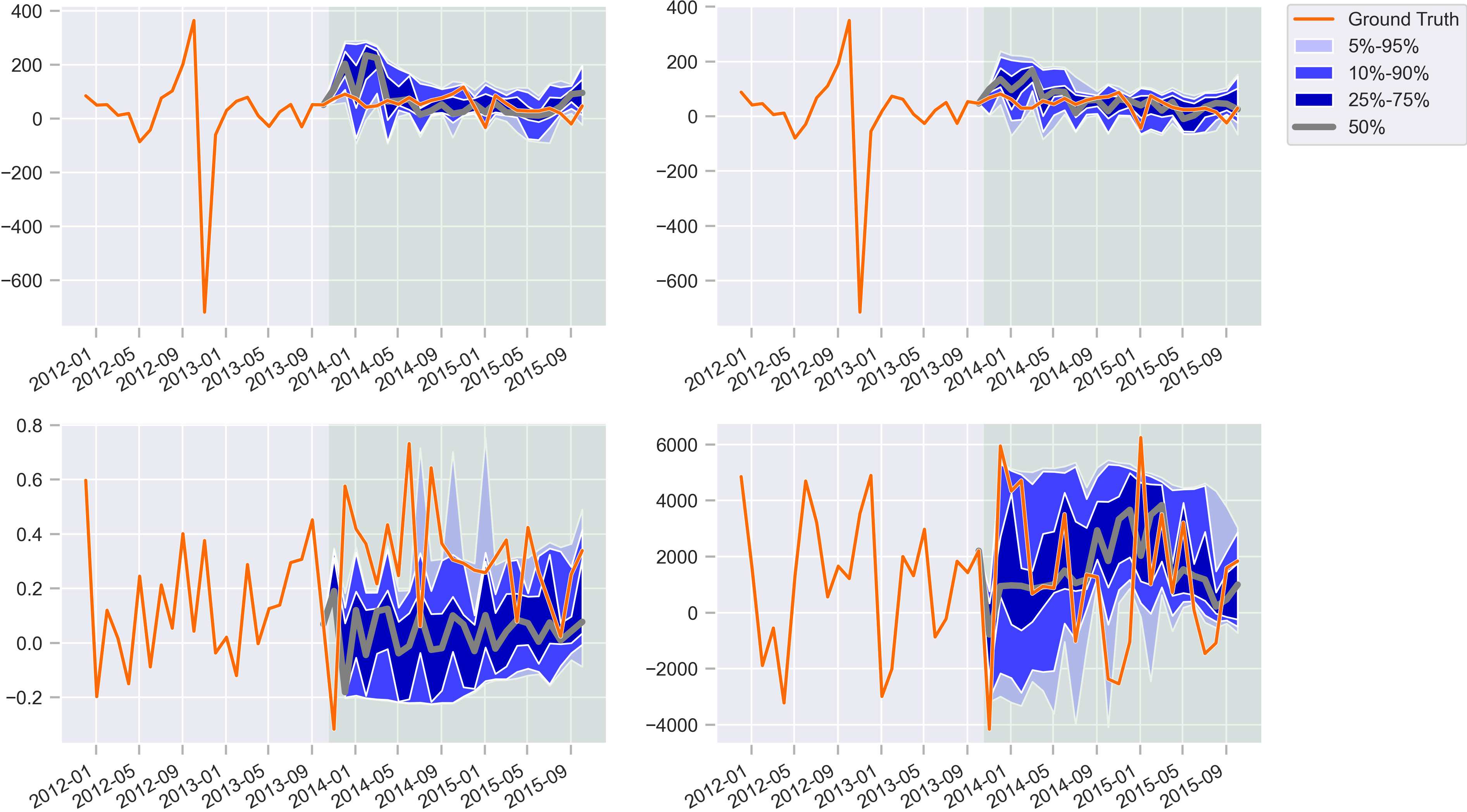
Figure 4: The predicted samples by the PrACTiS model for two-year forecasts, corresponding to $24$ time-steps, conditioned on two-year historical data in fred-md dataset.

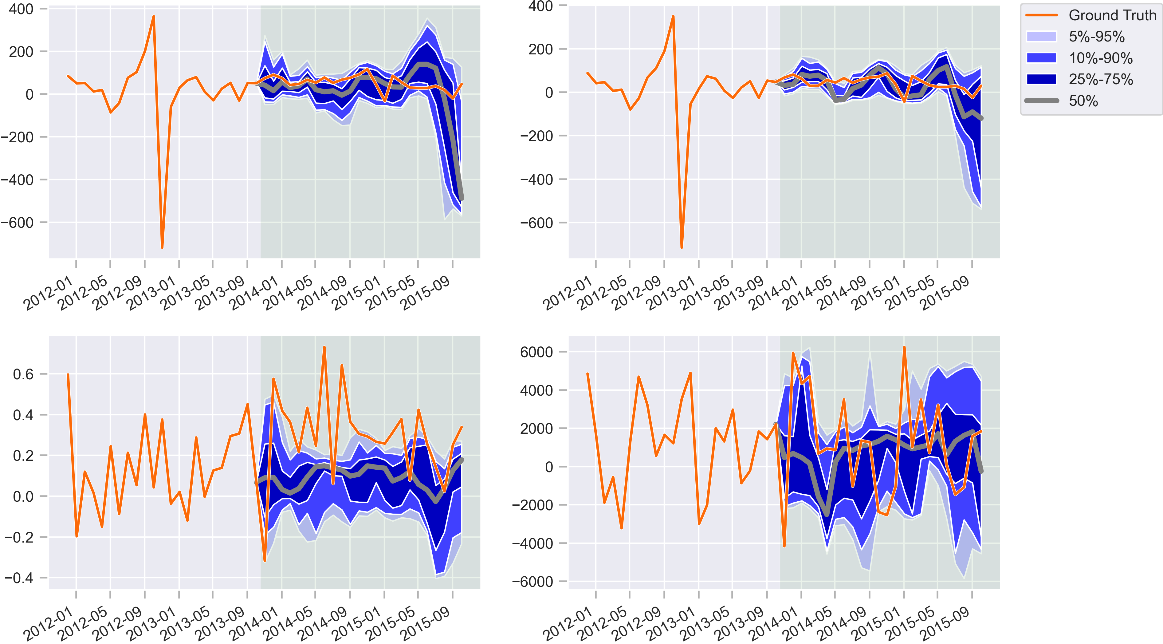
Figure 5: The predicted samples by the TACTiS model for two-year forecasts, corresponding to $24$ time-steps, conditioned on two-year historical data in fred-md dataset.

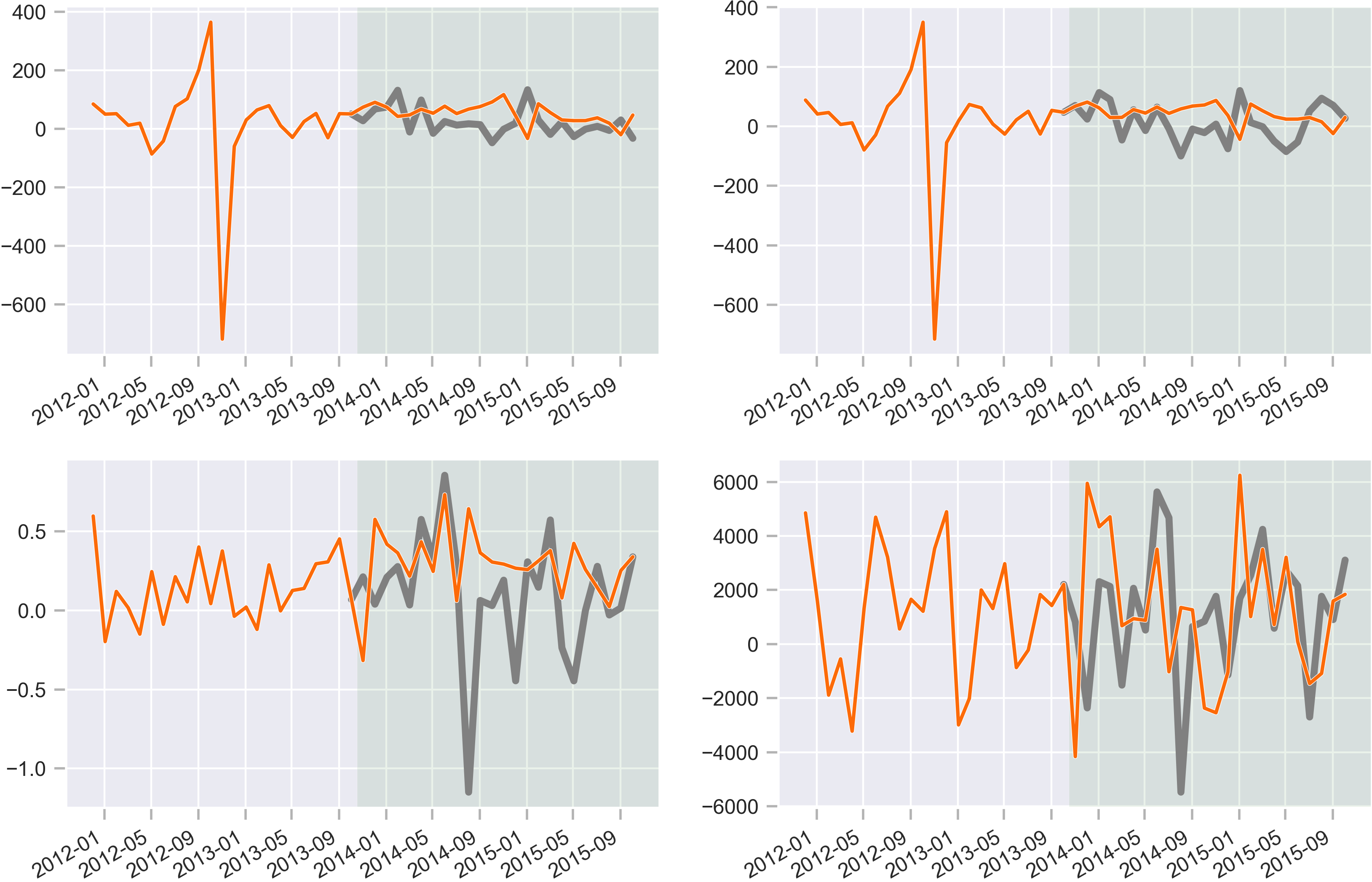
Figure 6: The predicted samples by the AR(24) model for two-year forecasts, corresponding to $24$ time-steps, conditioned on two-year historical data in fred-md dataset.

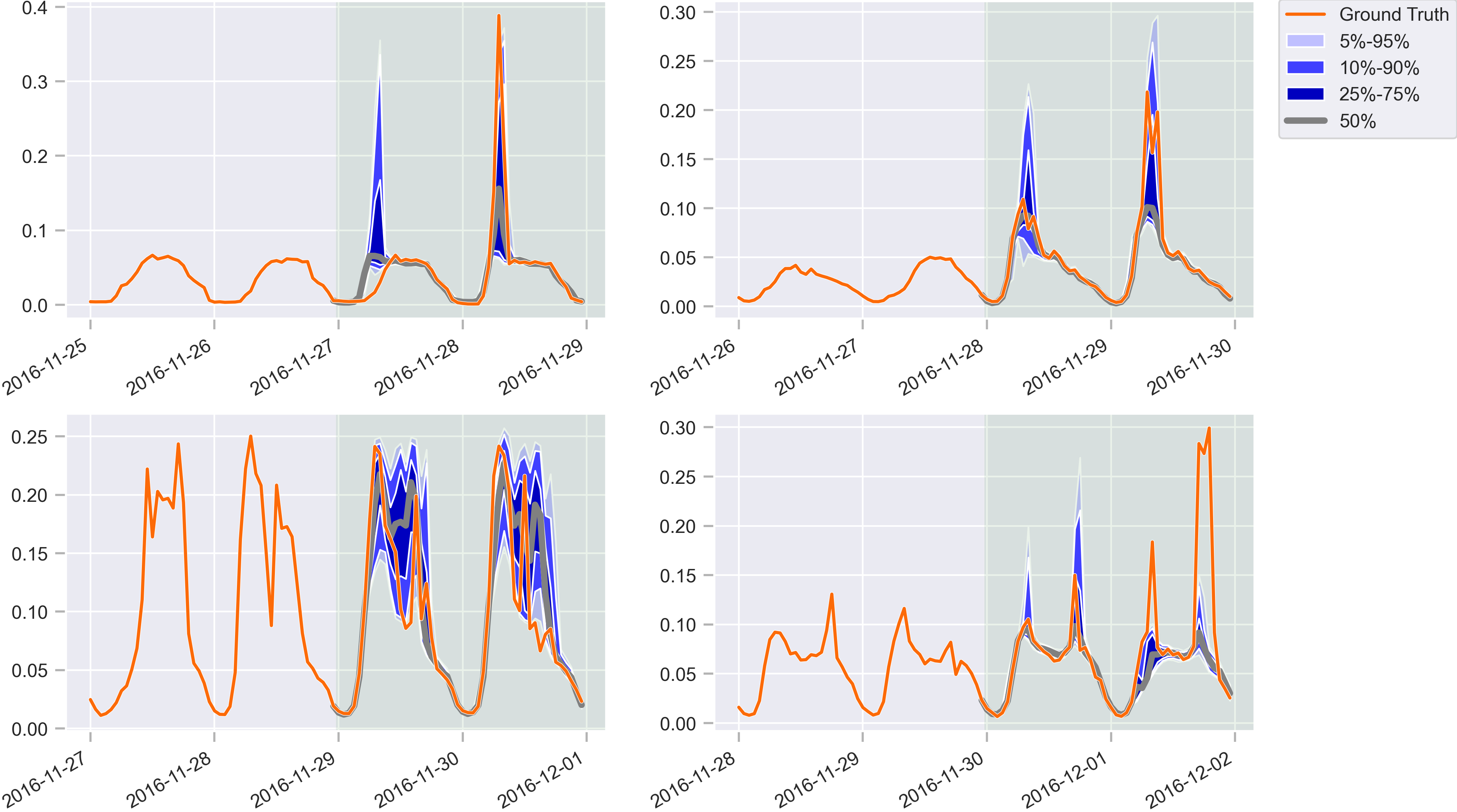
Figure 7: The predicted samples by the PrACTiS model for two-day forecasts, corresponding to $48$ time-steps, conditioned on two-day historical data in traffic dataset.

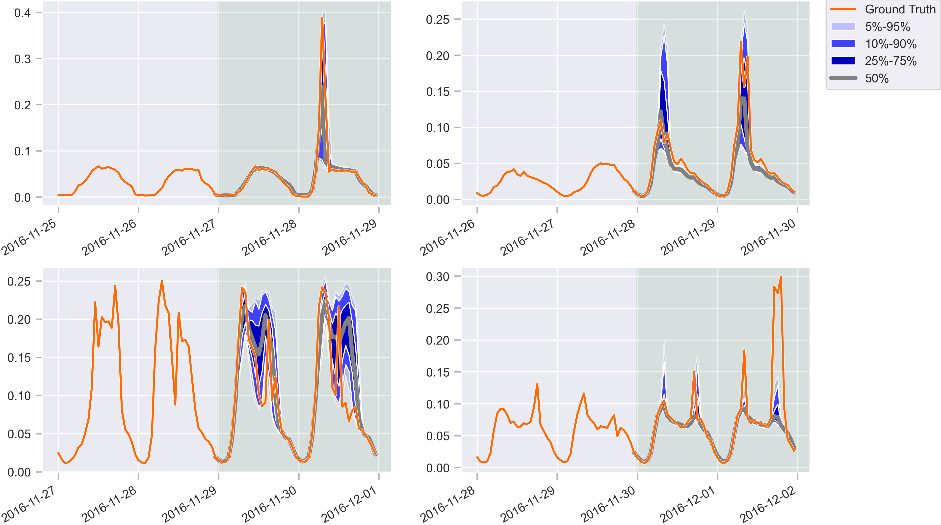
Figure 8: The predicted samples by the TACTiS model for two-day forecasts, corresponding to $48$ time-steps, conditioned on two-day historical data in traffic dataset.

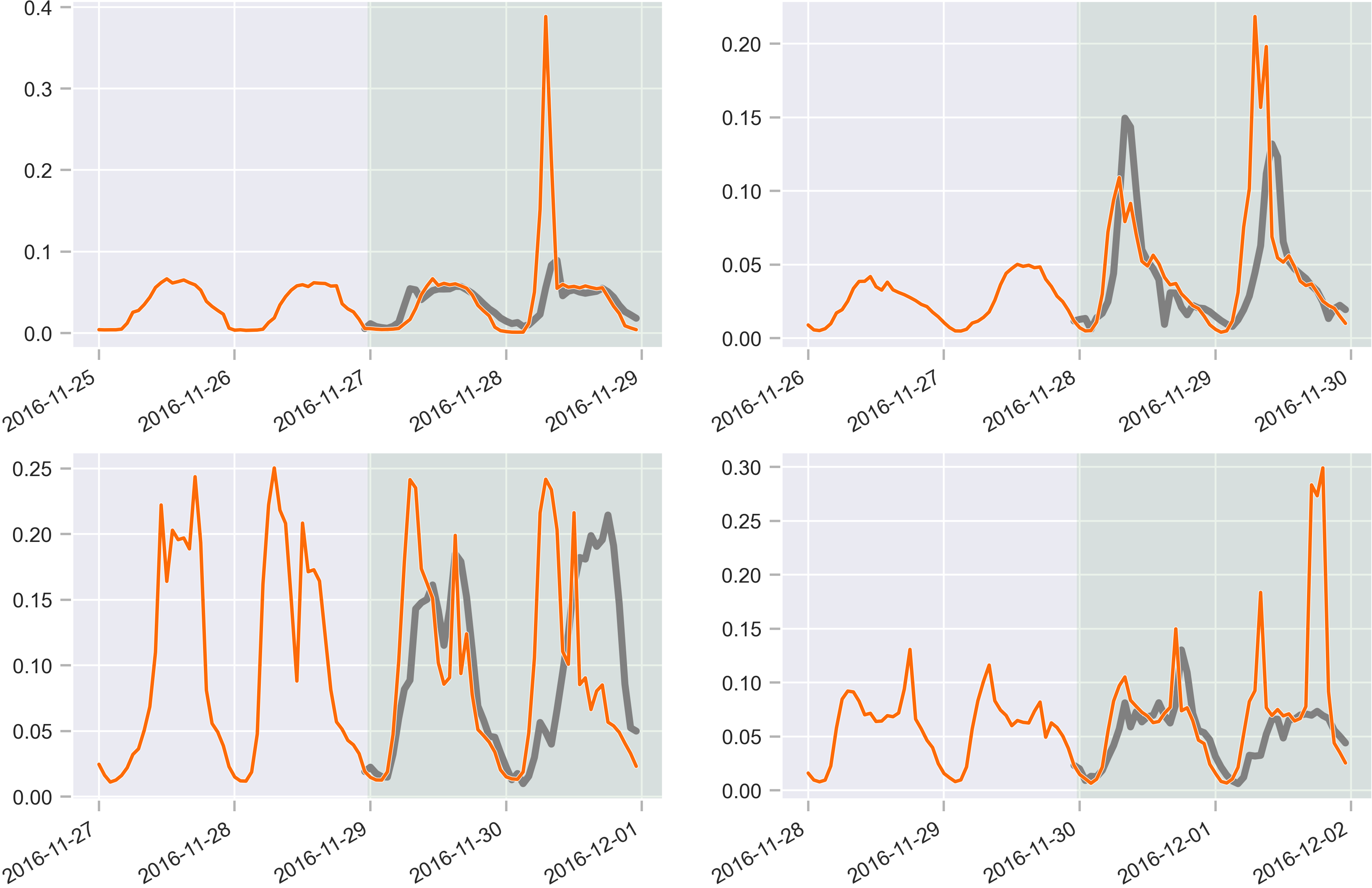
Figure 9: The predicted samples by the AR(48) model for two-day forecasts, corresponding to $48$ time-steps, conditioned on two-day historical data in traffic dataset.

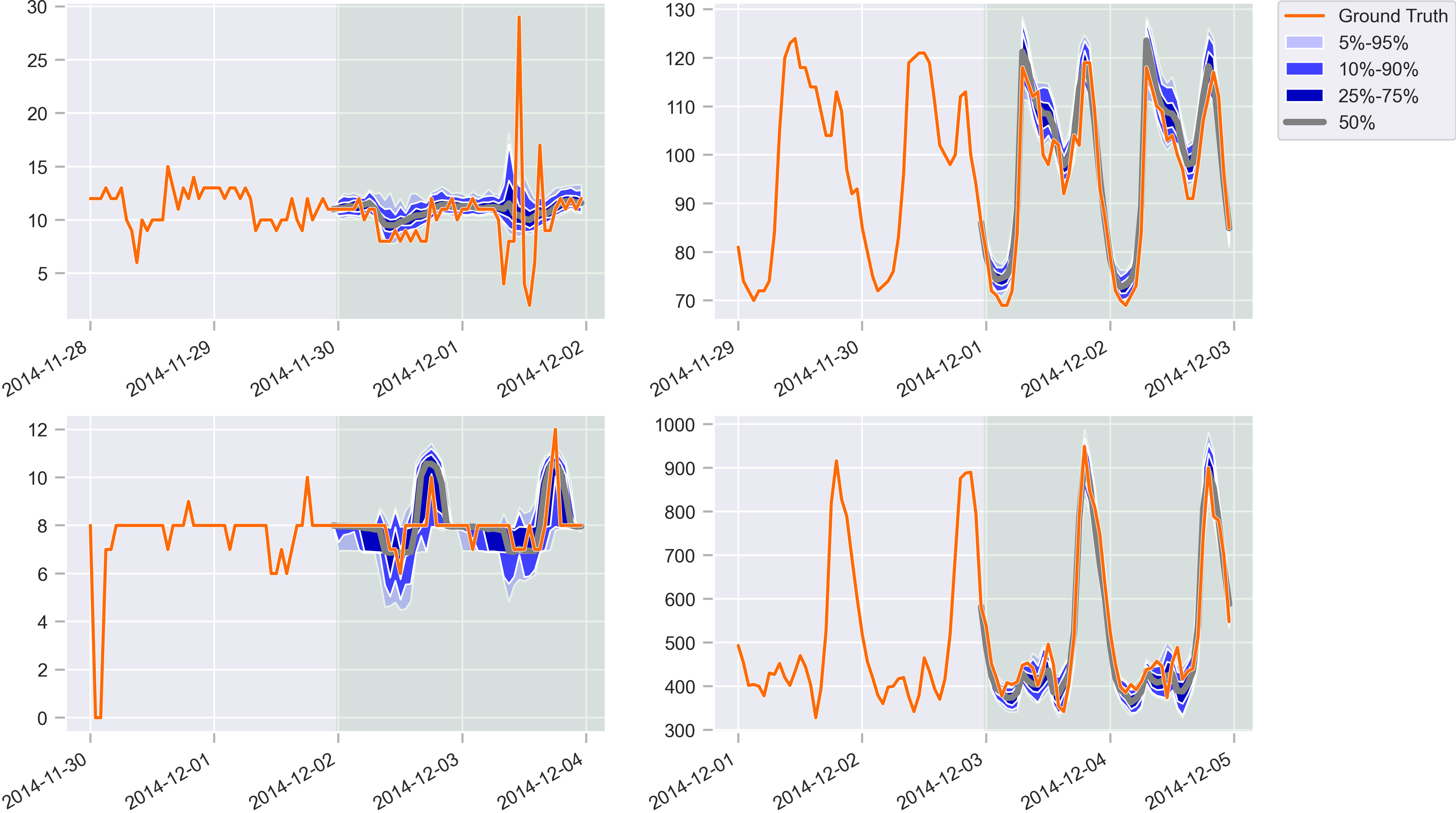
Figure 10: The predicted samples by the PrACTiS model for two-day forecasts, corresponding to $48$ time-steps, conditioned on two-day historical data in electricity dataset.

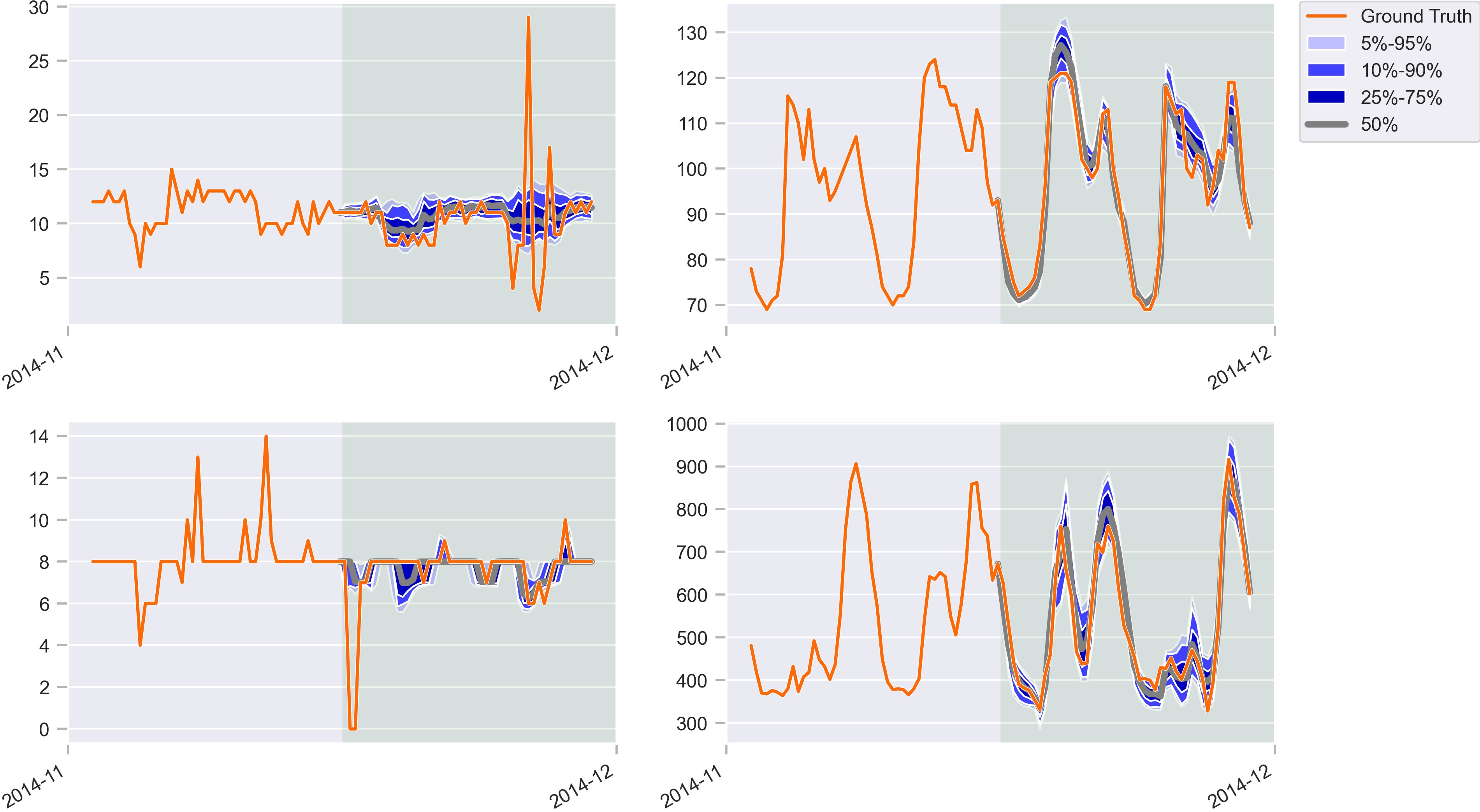
Figure 11: The predicted samples by the TACTiS model for two-day forecasts, corresponding to $48$ time-steps, conditioned on two-day historical data in electricity dataset.

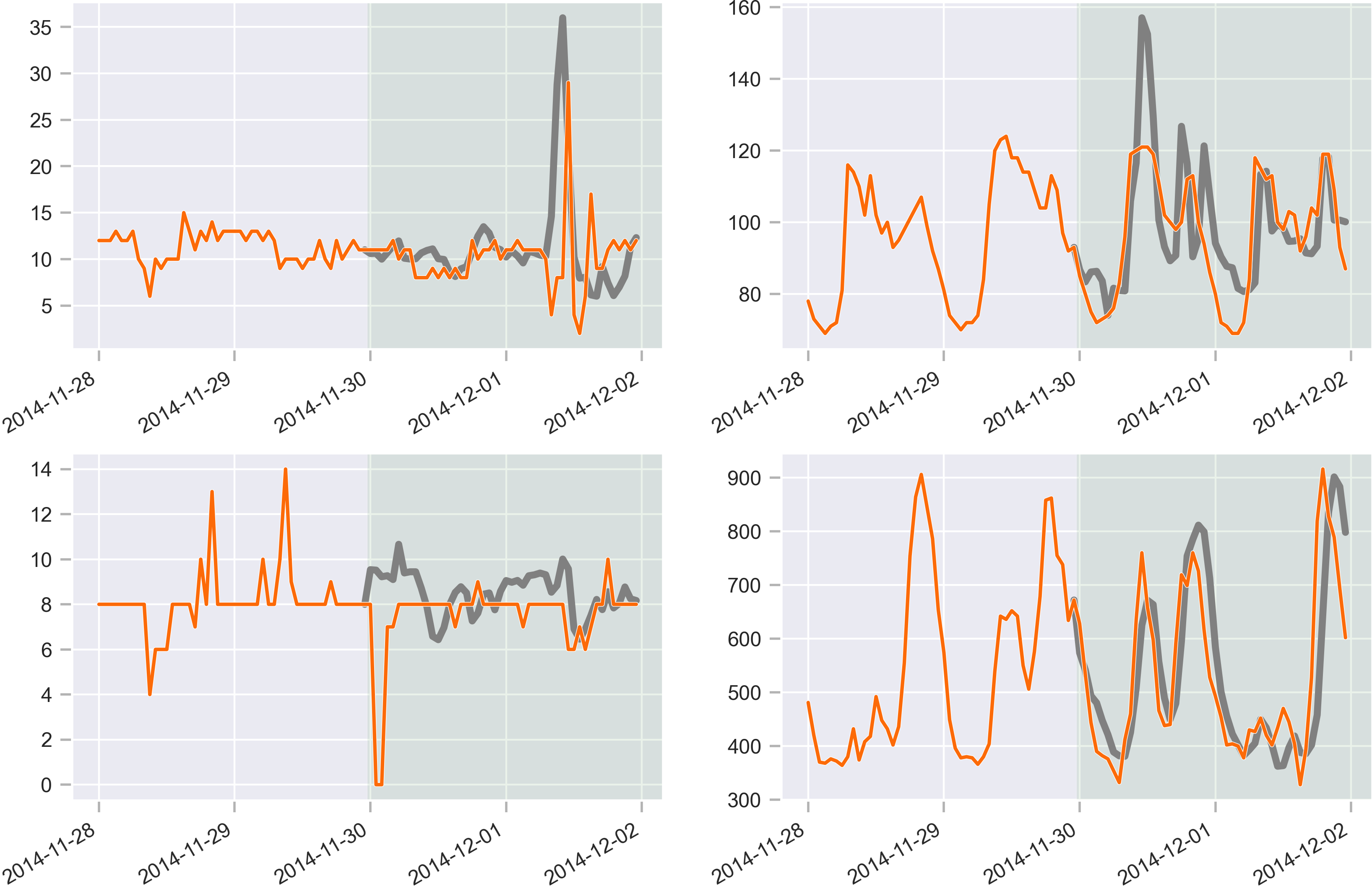
Figure 12: The predicted samples by the AR(48) model for two-day forecasts, corresponding to $48$ time-steps, conditioned on two-day historical data in electricity dataset.

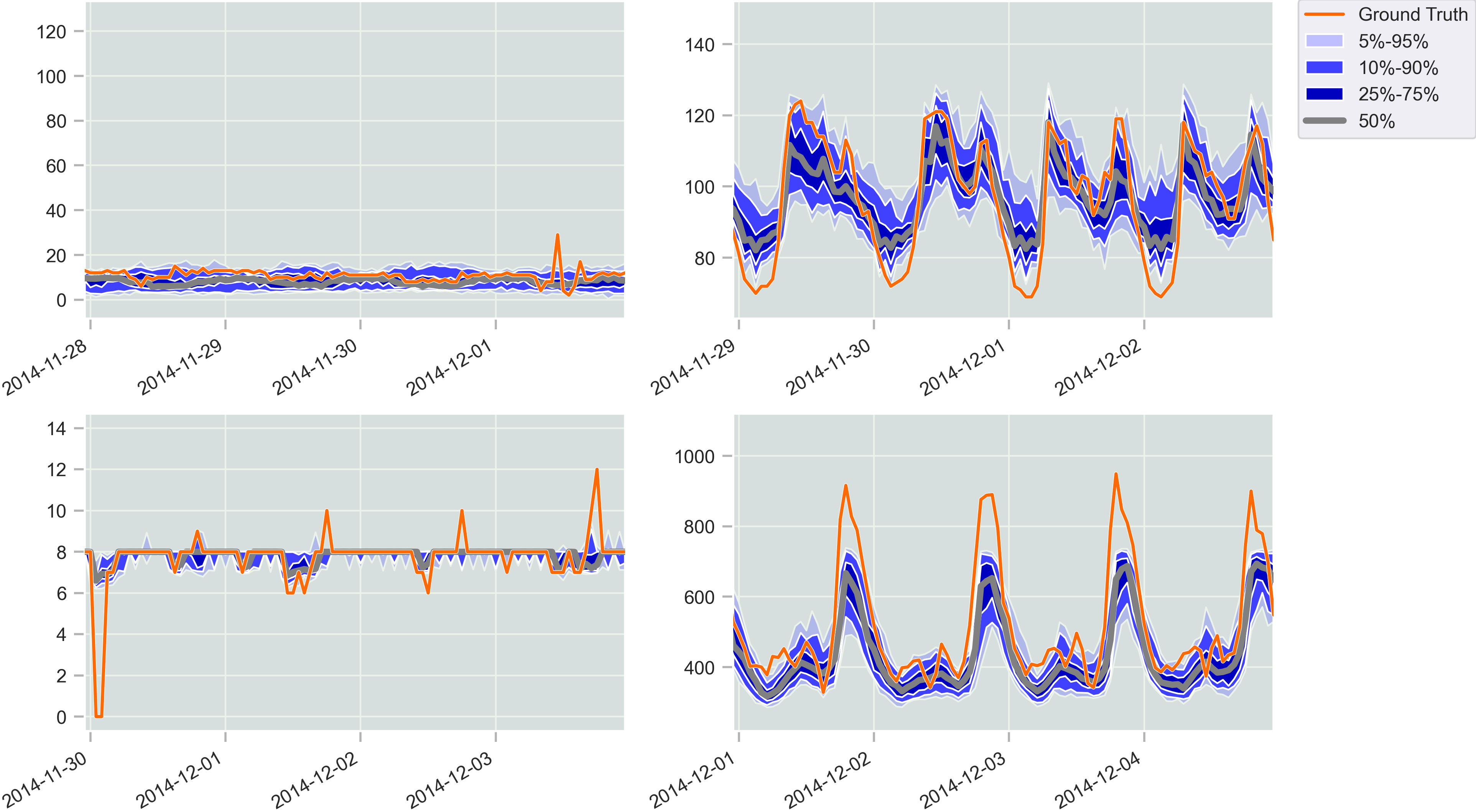
Figure 13: The final four-day predicted samples by the PrACTiS model for one-month forecasts, corresponding to $672$ time-steps, conditioned on one-month historical data in electricity dataset.

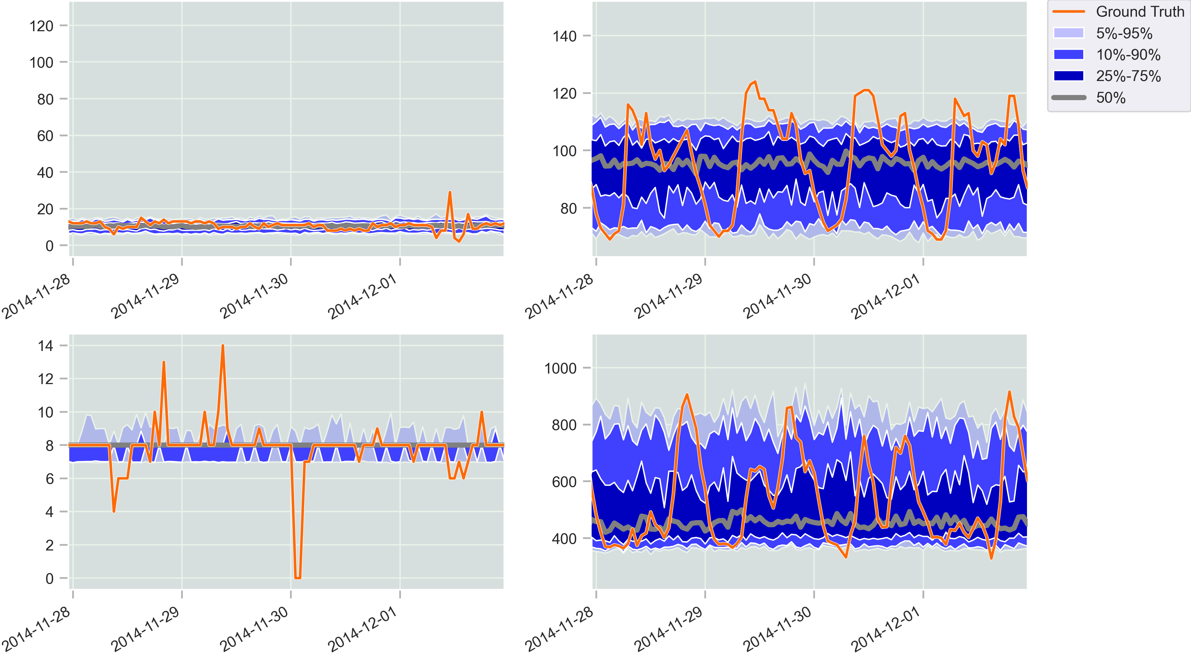
Figure 14: The final four-day predicted samples by the TACTiS model for one-month forecasts, corresponding to $672$ time-steps, conditioned on one-month historical data in electricity dataset.

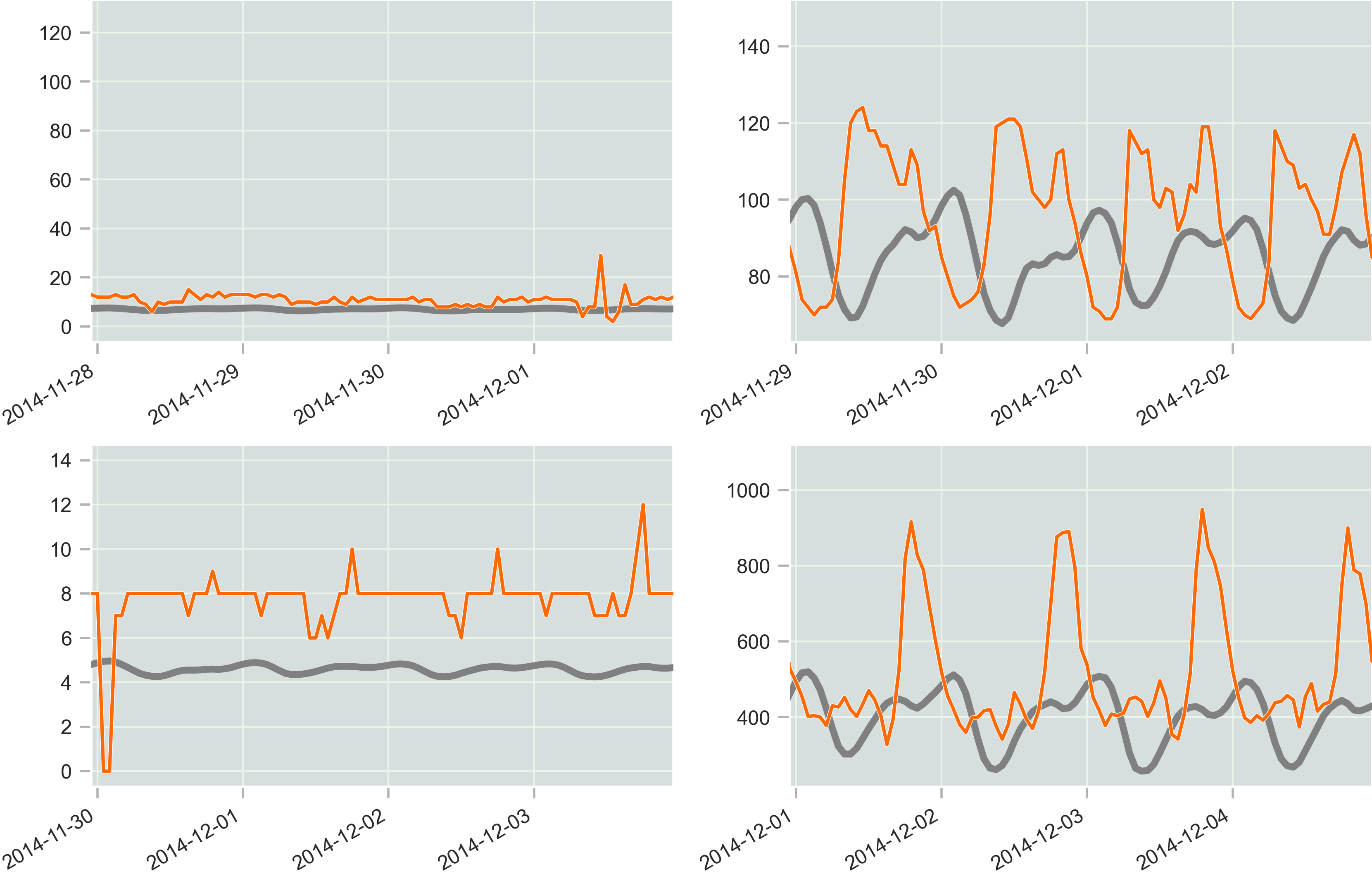
Figure 15: The final four-day predicted samples by the AR(672) model for one-month forecasts, corresponding to $672$ time-steps, conditioned on one-month historical data in electricity dataset.

References

- Aas et al. (2009) Kjersti Aas, Claudia Czado, Arnoldo Frigessi, and Henrik Bakken. Pair-copula constructions of multiple dependence. Insurance: Mathematics and economics, 44(2):182–198, 2009.
- Benidis et al. (2022) Konstantinos Benidis, Syama Sundar Rangapuram, Valentin Flunkert, Yuyang Wang, Danielle Maddix, Caner Turkmen, Jan Gasthaus, Michael Bohlke-Schneider, David Salinas, Lorenzo Stella, et al. Deep learning for time series forecasting: Tutorial and literature survey. ACM Computing Surveys, 55(6):1–36, 2022.
- Box et al. (2015) George EP Box, Gwilym M Jenkins, Gregory C Reinsel, and Greta M Ljung. Time series analysis: forecasting and control. John Wiley & Sons, 2015.
- Candanedo (2016) Luis Candanedo. Occupancy Detection . UCI Machine Learning Repository, 2016. DOI: https://doi.org/10.24432/C5X01N.
- Chapados & Bengio (2007) Nicolas Chapados and Yoshua Bengio. Augmented functional time series representation and forecasting with gaussian processes. Advances in neural information processing systems, 20, 2007.
- Chen (2019) Song Chen. Beijing Multi-Site Air-Quality Data. UCI Machine Learning Repository, 2019. DOI: https://doi.org/10.24432/C5RK5G.
- Chen et al. (2020) Yitian Chen, Yanfei Kang, Yixiong Chen, and Zizhuo Wang. Probabilistic forecasting with temporal convolutional neural network. Neurocomputing, 399:491–501, 2020.
- Child et al. (2019) Rewon Child, Scott Gray, Alec Radford, and Ilya Sutskever. Generating Long Sequences with Sparse Transformers. arXiv preprint arXiv:1904.10509, 2019.
- Connor et al. (1994) Jerome T Connor, R Douglas Martin, and Les E Atlas. Recurrent neural networks and robust time series prediction. IEEE transactions on neural networks, 5(2):240–254, 1994.
- de Bézenac et al. (2020) Emmanuel de Bézenac, Syama Sundar Rangapuram, Konstantinos Benidis, Michael Bohlke-Schneider, Richard Kurle, Lorenzo Stella, Hilaf Hasson, Patrick Gallinari, and Tim Januschowski. Normalizing kalman filters for multivariate time series analysis. Advances in Neural Information Processing Systems, 33:2995–3007, 2020.
- Drouin et al. (2022) Alexandre Drouin, Étienne Marcotte, and Nicolas Chapados. TACTiS: Transformer-Attentional Copulas for Time Series. In International Conference on Machine Learning, pp. 5447–5493. PMLR, 2022.
- Dua & Graff (2017) Dheeru Dua and Casey Graff. Uci machine learning repository, 2017. URL http://archive.ics.uci.edu/ml.
- Godahewa et al. (2021) Rakshitha Godahewa, Christoph Bergmeir, Geoffrey I Webb, Rob J Hyndman, and Pablo Montero-Manso. Monash time series forecasting archive. arXiv preprint arXiv:2105.06643, 2021.
- Größer & Okhrin (2022) Joshua Größer and Ostap Okhrin. Copulae: An overview and recent developments. Wiley Interdisciplinary Reviews: Computational Statistics, 14(3):e1557, 2022.
- Hinton et al. (2012) Geoffrey Hinton, Nitish Srivastava, and Kevin Swersky. Neural Networks for Machine Learning Lecture 6A Overview of Mini-Batch Gradient Descent. Cited on, 14(8):2, 2012.
- Hochreiter & Schmidhuber (1997) Sepp Hochreiter and Jürgen Schmidhuber. Long short-term memory. Neural computation, 9(8):1735–1780, 1997.
- Hogue (2019) John Hogue. Metro Interstate Traffic Volume. UCI Machine Learning Repository, 2019. DOI: https://doi.org/10.24432/C5X60B.
- Huang et al. (2018) Chin-Wei Huang, David Krueger, Alexandre Lacoste, and Aaron Courville. Neural autoregressive flows. In International Conference on Machine Learning, pp. 2078–2087. PMLR, 2018.
- Hyndman et al. (2008) Rob Hyndman, Anne B Koehler, J Keith Ord, and Ralph D Snyder. Forecasting with exponential smoothing: the state space approach. Springer Science & Business Media, 2008.
- Jaegle et al. (2021a) Andrew Jaegle, Sebastian Borgeaud, Jean-Baptiste Alayrac, Carl Doersch, Catalin Ionescu, David Ding, Skanda Koppula, Daniel Zoran, Andrew Brock, Evan Shelhamer, et al. Perceiver IO: A General Architecture for Structured Inputs & Outputs. arXiv preprint arXiv:2107.14795, 2021a.
- Jaegle et al. (2021b) Andrew Jaegle, Felix Gimeno, Andy Brock, Oriol Vinyals, Andrew Zisserman, and Joao Carreira. Perceiver: General Perception with Iterative Attention. In International Conference on Machine Learning, pp. 4651–4664. PMLR, 2021b.
- Kalliovirta et al. (2015) Leena Kalliovirta, Mika Meitz, and Pentti Saikkonen. A gaussian mixture autoregressive model for univariate time series. Journal of Time Series Analysis, 36(2):247–266, 2015.
- Krupskii & Joe (2013) Pavel Krupskii and Harry Joe. Factor copula models for multivariate data. Journal of Multivariate Analysis, 120:85–101, 2013.
- Krupskii & Joe (2020) Pavel Krupskii and Harry Joe. Flexible copula models with dynamic dependence and application to financial data. Econometrics and Statistics, 16:148–167, 2020.
- Le Guen & Thome (2020) Vincent Le Guen and Nicolas Thome. Probabilistic time series forecasting with shape and temporal diversity. Advances in Neural Information Processing Systems, 33:4427–4440, 2020.
- Li et al. (2019) Shiyang Li, Xiaoyong Jin, Yao Xuan, Xiyou Zhou, Wenhu Chen, Yu-Xiang Wang, and Xifeng Yan. Enhancing the locality and breaking the memory bottleneck of transformer on time series forecasting. Advances in neural information processing systems, 32, 2019.
- Lim & Zohren (2021) Bryan Lim and Stefan Zohren. Time-series forecasting with deep learning: a survey. Philosophical Transactions of the Royal Society A, 379(2194):20200209, 2021.
- Lim et al. (2021) Bryan Lim, Sercan Ö Arık, Nicolas Loeff, and Tomas Pfister. Temporal fusion transformers for interpretable multi-horizon time series forecasting. International Journal of Forecasting, 37(4):1748–1764, 2021.
- Liu et al. (2019) Yukai Liu, Rose Yu, Stephan Zheng, Eric Zhan, and Yisong Yue. NAOMI: Non-Autoregressive Multiresolution Sequence Imputation. Advances in Neural Information Processing Systems, 32, 2019.
- Lopez-Paz et al. (2012) David Lopez-Paz, Jose Hernández-lobato, and Bernhard Schölkopf. Semi-supervised domain adaptation with non-parametric copulas. Advances in neural information processing systems, 25, 2012.
- Mayer & Wied (2023) Alexander Mayer and Dominik Wied. Estimation and inference in factor copula models with exogenous covariates. Journal of Econometrics, 2023.
- Müller et al. (2021) Samuel Müller, Noah Hollmann, Sebastian Pineda Arango, Josif Grabocka, and Frank Hutter. Transformers can do bayesian inference. arXiv preprint arXiv:2112.10510, 2021.
- Nelsen (2006) Roger B Nelsen. An introduction to copulas. Springer, 2006.
- Oh & Patton (2017) Dong Hwan Oh and Andrew J Patton. Modeling dependence in high dimensions with factor copulas. Journal of Business & Economic Statistics, 35(1):139–154, 2017.
- Oreshkin et al. (2019) Boris N Oreshkin, Dmitri Carpov, Nicolas Chapados, and Yoshua Bengio. N-beats: Neural basis expansion analysis for interpretable time series forecasting. arXiv preprint arXiv:1905.10437, 2019.
- Patton (2012) Andrew J Patton. A review of copula models for economic time series. Journal of Multivariate Analysis, 110:4–18, 2012.
- Roy et al. (2021) Aurko Roy, Mohammad Saffar, Ashish Vaswani, and David Grangier. Efficient Content-Based Sparse Attention with Routing Transformers. Transactions of the Association for Computational Linguistics, 9:53–68, 2021.
- Salinas et al. (2019) David Salinas, Michael Bohlke-Schneider, Laurent Callot, Roberto Medico, and Jan Gasthaus. High-Dimensional Multivariate Forecasting with Low-Rank Gaussian Copula Processes. Advances in Neural Information Processing Systems, 32, 2019.
- Shih et al. (2019) Shun-Yao Shih, Fan-Keng Sun, and Hung-yi Lee. Temporal pattern attention for multivariate time series forecasting. Machine Learning, 108:1421–1441, 2019.
- Shukla & Marlin (2021) Satya Narayan Shukla and Benjamin M Marlin. Multi-time attention networks for irregularly sampled time series. arXiv preprint arXiv:2101.10318, 2021.
- Sklar (1959) M Sklar. Fonctions de repartition an dimensions et leurs marges publications de l’institut de statistique de l’universite de paris, vol. 8. 1959.
- Tashiro et al. (2021) Yusuke Tashiro, Jiaming Song, Yang Song, and Stefano Ermon. Csdi: Conditional score-based diffusion models for probabilistic time series imputation. Advances in Neural Information Processing Systems, 34:24804–24816, 2021.
- Tay et al. (2020) Yi Tay, Dara Bahri, Liu Yang, Donald Metzler, and Da-Cheng Juan. Sparse Sinkhorn Attention. In International Conference on Machine Learning, pp. 9438–9447. PMLR, 2020.
- Vaswani et al. (2017) Ashish Vaswani, Noam Shazeer, Niki Parmar, Jakob Uszkoreit, Llion Jones, Aidan N Gomez, Łukasz Kaiser, and Illia Polosukhin. Attention Is All You Need. Advances in Neural Information Processing Systems, 30, 2017.
- Yanchenko & Mukherjee (2020) Anna K Yanchenko and Sayan Mukherjee. Stanza: a nonlinear state space model for probabilistic inference in non-stationary time series. arXiv preprint arXiv:2006.06553, 2020.
- Zhang et al. (1998) Guoqiang Zhang, B Eddy Patuwo, and Michael Y Hu. Forecasting with artificial neural networks:: The state of the art. International journal of forecasting, 14(1):35–62, 1998.
- Zhu et al. (2021) Qiding Zhu, Shukui Zhang, Yang Zhang, Chunqing Yu, Mengli Dang, and Li Zhang. Multimodal time series data fusion based on ssae and lstm. In 2021 IEEE Wireless Communications and Networking Conference (WCNC), pp. 1–7. IEEE, 2021.