Ensemble Distillation for Unsupervised Constituency Parsing

Abstract

We investigate the unsupervised constituency parsing task, which organizes words and phrases of a sentence into a hierarchical structure without using linguistically annotated data. We observe that existing unsupervised parsers capture differing aspects of parsing structures, which can be leveraged to enhance unsupervised parsing performance. To this end, we propose a notion of “tree averaging,” based on which we further propose a novel ensemble method for unsupervised parsing. To improve inference efficiency, we further distill the ensemble knowledge into a student model; such an ensemble-then-distill process is an effective approach to mitigate the over-smoothing problem existing in common multi-teacher distilling methods. Experiments show that our method surpasses all previous approaches, consistently demonstrating its effectiveness and robustness across various runs, with different ensemble components, and under domain-shift conditions.

1 Introduction

Constituency parsing is a core task in natural language processing (NLP), which interprets a sentence and induces its constituency tree, a syntactic structure representation that organizes words and phrases into a hierarchy (Carnie, 2007). It has wide applications in various downstream tasks, including semantic role labeling (Mohammadshahi and Henderson, 2023) and explainability of AI models (Tenney et al., 2019). Traditionally, parsing is accomplished by supervised models trained with linguistically annotated treebanks (Charniak, 2000), which are expensive to obtain and may not be available for low-resource scenarios. Also, these supervised parsers often underperform when encountering domain shifts. This motivates researchers to explore unsupervised methods as it eliminates the need for annotated data.

To address unsupervised parsing, researchers have proposed various heuristics and indirect supervision signals. Clark (2001) employs context distribution clustering to induce a probabilistic context-free grammar (PCFG; Booth, 1969). Klein and Manning (2002) define a joint distribution for sentences and parse structures, the latter learned by expectation–maximization (EM) algorithms. Snyder et al. (2009) address multilingual unsupervised parsing by aligning potential parse trees in a generative model.

In the deep learning era, unsupervised parsing techniques keep advancing. Cao et al. (2020) utilize linguistic constituency tests (Fromkin et al., 2003) as heuristics, evaluating all spans as potential constituents for selection. Li and Lu (2023) modify each span based on linguistic perturbations and observe changes in the contextual representations within a masked language model; according to the level of distortion, they determine how likely the span is a constituent. Maveli and Cohen (2022) use rules to train two classifiers with local features and contextual features, respectively, which are further refined in a co-training fashion. Another way to obtain the parsing structure in an unsupervised way is to treat it as a latent variable and train it in downstream tasks, such as text classification (Li et al., 2019), language modeling (Shen et al., 2019; Kim et al., 2019b), and sentence reconstruction (Drozdov et al., 2019; Kim et al., 2019a). Overall, unsupervised parsing is made feasible by such heuristics and indirect supervisions, and has become a curious research direction in NLP.

In our work, we uncover an intriguing phenomenon of low correlation among different unsupervised parsers, despite their similar overall $F_{1}$ scores (the main evaluation metric for parsing), shown in Table 1. This suggests that different approaches capture different aspects of parsing structures, and our insight is that combining these parsers may leverage their different expertise, achieving higher performance for unsupervised parsing.

To this end, we propose an ensemble method for unsupervised parsing. We first introduce a notion of “tree averaging” based on the similarity of two constituency trees. Given a few existing unsupervised parsers, referred to as teachers, we then propose to use a CYK-like algorithm (Kasami, 1966; Younger, 1967; Manacher, 1978; Sennrich, 2014) that utilizes dynamic programming to search for the tree that is most similar to all teachers’ outputs. In this way, we are able to obtain an “average” parse tree, taking advantage of different existing unsupervised parsers.

To improve the inference efficiency, we distill our ensemble knowledge into a student model. In particular, we choose the recurrent neural network grammar (RNNG; Dyer et al., 2016) with an unsupervised self-training procedure (URNNG; Kim et al., 2019b), following the common practice in unsupervised parsing (Kim et al., 2019a; Cao et al., 2020). Our ensemble-then-distill process is able to mitigate the over-smoothing problem, where the standard cross-entropy loss encourages the student to learn an overly smooth distribution (Wen et al., 2023). Such a problem exists in common multi-teacher distilling methods (Wu et al., 2021), and it would be especially severe when the teachers are heterogeneous, signifying the importance of our approach.

We evaluated our ensemble method on the Penn Treebank (PTB; Marcus et al., 1993) and SUSANNE (Sampson, 2002) corpora. Results show that our approach outperforms existing unsupervised parsers by a large margin in terms of $F_{1}$ scores, and that it achieves results comparable to the supervised counterpart in the domain-shift setting. Overall, our paper largely bridges the gap between supervised and unsupervised parsing.

In short, the main contributions of this paper include: 1) We reveal an intriguing phenomenon that existing unsupervised parsers have diverse expertise, which may be leveraged by model ensembles; 2) We propose a notion of tree averaging and utilize a CYK-like algorithm that searches for the average tree of existing unsupervised parsers; and 3) We propose an ensemble-then-distill approach to improve inference efficiency and to alleviate the over-smoothing problem in common multi-teacher distilling approaches.

Compound PCFG	$100$
DIORA	$55.8$	$100$
S-DIORA	$58.1$	$63.6$	$100$
	Compound	DIORA	S-DIORA
	PCFG

DIORA✩	$100$
DIORA✧	$74.1$	$100$
DIORA✻	$74.3$	$74.9$	$100$
	DIORA✩	DIORA✧	DIORA✻

Table 1: Correlation analysis of unsupervised parsers. Numbers are the $F_{1}$ score of one model against another on the Penn Treebank dataset (Marcus et al., 1993). The left table considers three heterogeneous models (Compound PCFG, DIORA, and S-DIORA), whereas the right table considers three runs (✩, ✧, and ✻) of the same model. All their $F_{1}$ scores against the ground truth fall within the range of 59–61, thus providing a controlled experimental setting.

2 Approach

2.1 Unsupervised Constituency Parsing

In linguistics, a constituent refers to a word or a group of words that function as a single unit in a hierarchical tree structure (Carnie, 2007). In the sentence “The quick brown fox jumps over the lazy dog,” for example, the phrase “the lazy dog” serves as a noun phrase constituent, whereas “jumps over the lazy dog” is a verb phrase constituent. In this study, we address unsupervised constituency parsing, where no linguistic annotations are used for training. This reduces human labor and is potentially useful for low-resource languages. Following most previous work in this direction (Cao et al., 2020; Maveli and Cohen, 2022; Li and Lu, 2023), we focus on unlabeled, binary parse trees, in which each constituent has a binary branching and is not labeled with its syntactic role (such as a noun phrase or a verb phrase).

The standard evaluation metric for constituency parsing is the $F_{1}$ score, which is the harmonic mean of precision and recall (Shen et al., 2018; Zhang et al., 2021):

$$P=\frac{|C(T_{\text{pred}})\cap C(T_{\text{ref}})|}{|C(T_{\text{pred}})|},\;\;R=\frac{|C(T_{\text{pred}})\cap C(T_{\text{ref}})|}{|C(T_{\text{ref}})|},\;\;F_{1}=2\frac{PR}{P+R}$$ (1)

where $T_{\text{pred}}$ and $T_{\text{ref}}$ are predicted and reference trees, respectively, and $C(T)$ is the set of constituents of a tree $T$.

2.2 A Notion of Averaging Constituency Trees

In our study, we propose an ensemble approach to combine the expertise of existing unsupervised parsers (called teachers), as we observe they have low correlation among themselves despite their similar overall $F_{1}$ scores (Table 1).

To accomplish ensemble binary constituency parsing, we need to define a notion of tree averaging; i.e., our ensemble output is the average tree that is most similar to all teachers’ outputs. Inspired by the evaluation metric, we suggest the average tree should have the highest total $F_{1}$ score compared with different teachers. Let $s$ be a sentence and $T_{k}$ is the $k$th teacher parser. Given $K$ teachers, we define the average tree to be

$$\operatorname{AvgTree}(s,\{T_{k}\}_{k=1}^{K})=\operatorname*{arg\,max}\limits_{T\in\mathcal{T}(s)}\sum_{k=1}^{K}F_{1}(T,T_{k}(s))$$ (2)

where $\mathcal{T}(s)$ is all possible unlabeled binary trees on sentence $s$, and $T_{k}(s)$ is the $k$th teacher’s output.

It is emphasized that only the trees of the same sentence can be averaged. This simplifies the $F_{1}$ score of binary trees, as the denominators for both precision and recall are $2|s|-1$ for a sentence with $|s|$ words, i.e., $|C(T_{\text{pred}})|=|C(T_{\text{ref}})|=2|s|-1$. Thus, Eqn. (2) can be rewritten as:

$$\operatorname{AvgTree}(s,\{T_{k}\}_{k=1}^{K}) =\operatorname*{arg\,max}\limits_{T\in\mathcal{T}(s)}\sum_{k=1}^{K}F_{1}(T,T_{k}(s))=\operatorname*{arg\,max}\limits_{T\in\mathcal{T}(s)}\sum_{k=1}^{K}\frac{|C(T)\cap C(T_{k}(s))|}{2|s|-1}$$ (3)

$$=\operatorname*{arg\,max}\limits_{T\in\mathcal{T}(s)}\sum_{c\in C(T)}\underbrace{\sum_{k=1}^{K}\mathds{1}[c\in C(T_{k}(s))]}_{\operatorname{HitCount}(c,\{T_{k}(s)\}_{k=1}^{K})}$$ (4)

Here, we define the $\operatorname{HitCount}$ function to be the number of times that a constituent $c$ appears in the teachers’ outputs. In other words, Eqn. (4) suggests that the best averaging tree should be the one that hits the teachers’ predicted constituents most.

Discussion on MBR decoding. Our work can be seen as minimum Bayes risk (MBR) decoding (Bickel and Doksum, 2015). In general, MBR yields an output that minimizes an expected error (called Bayes risk), defined according to the task of interest. In our case, the error function can be thought of as $-\sum_{c\in C(T)}\operatorname{HitCount}(c,\{T_{k}(s)\}_{k=1}^{K})$, and minimizing such-defined Bayes risk is equivalent to maximizing the total hit counts, as shown by Eqn. (4).

However, our MBR approach significantly differs from prior MBR studies in NLP. In fact, MBR has been widely applied to text generation (Kumar and Byrne, 2004; Freitag et al., 2022; Suzgun et al., 2023), where a set of candidate output sentences are obtained by sampling or beam search, and the best one is selected based on a given error function, e.g., the dissimilarity against others; such an MBR method is selective, meaning that the output can only be selected from a candidate set. On the contrary, our MBR is generative, as the sentence’s entire parse space $\mathcal{T}(s)$ will be considered during the $\operatorname*{arg\,max}$ process in (4). This allows us to obtain the global lowest-risk tree and consequently achieve higher performance. Here, the global search is feasible because the nature of tree structures facilitates efficient exact decoding with dynamic programming, discussed in the next subsection.

2.3 Our CYK Variant

As indicated by Eqn. (4), our method searches for the constituency tree with the highest total hit counts of its constituents in the teachers’ outputs. We can achieve this by a CYK (Kasami, 1966; Younger, 1967)-like dynamic programming algorithm, because an optimal constituency parse structure of a span—a continuous subsequence of a sentence—is independent of the rest of the sentence.

Given a sentence $s$, we denote by $s_{b:e}$ a span starting from the $b$th word and ending right before the $e$th word. Considering a set of teachers $\{T_{k}\}_{k=1}^{K}$, we define a recursion variable

$$H_{b:e}=\max_{T\in\mathcal{T}({s_{b:e}})}\sum_{c\in C(T)}\operatorname{HitCount}(c,\{T_{k}(s)\}_{k=1}^{K})$$ (5)

which is the best total hit count for this span. We also define $L_{b:e}$ to be the corresponding locally best parse structure, unambiguously represented by the set of all constituents in it.

The base cases are $H_{b:b+1}=K$ and $L_{b:b+1}=\{s_{b:b+1}\}$ for $b=1,\cdots,|s|$, suggesting that the best parse tree of a single-word span is the word itself, which appears in all teachers’ outputs and has a hit count of $K$.

For recursion, we see a span $s_{b:e}$ will be split into two subspans $s_{b:j}$ and $s_{j:e}$ for some split position $j$, because our work focuses on binary constituency parsing. Given $j$, the total hit count for the span $s_{b:e}$ is the summation over those of the two subspans $s_{b:j}$ and $s_{j:e}$, plus its own hit count. To obtain the best split, we need to vary $j$ from $b$ to $e$ (exclusive), given by

$$j_{b:e}^{*}=\operatorname*{arg\,max}\limits_{b<j<e}\left[H_{b:j}+H_{j:e}+\operatorname{HitCount}(s_{b:e},\{T_{k}(s)\}_{k=1}^{K})\right]$$ (6)

where the hit count is a constant for $\operatorname*{arg\,max}$ and can be omitted in implementation. Then, we have

$$H_{b:e} =H_{b:j_{b:e}^{*}}+H_{j_{b:e}^{*}:e}+\operatorname{HitCount}(s_{b:e},\{T_{k}(s)\}_{k=1}^{K})$$ (7)

$$L_{b:e} =L_{b:j_{b:e}^{*}}\cup L_{j_{b:e}^{*}:e}\cup\{s_{b:e}\}$$ (8)

Eqn. (8) essentially groups two sub-parse structures $L_{b:j_{b:e}^{*}}$ and $L_{j_{b:e}^{*}:e}$ for the span $s_{b:e}$. This can be represented as the union operation on the sets of constituents.

The recursion terminates when we have computed $L_{1:|s|+1}$, which is the best parse tree for the sentence $s$, maximizing overall similarity to the teachers’ predictions and being our ensemble output. In Appendix A, we summarize our ensemble procedure in pseudocode and provide an illustration.

2.4 Ensemble Distillation

In our work, we further propose an ensemble distilling approach that trains a student parser from an ensemble of teachers. This is motivated by the fact that the ensemble model requires performing inference for all teacher models and may be slow. Specifically, we choose the recurrent neural network grammar (RNNG; Dyer et al., 2016) as the student model, which learns shift–reduce parsing operations (Aho and Johnson, 1974) along with language modeling using recurrent neural networks. The choice of RNNG is due to its unsupervised refinement procedure (URNNG; Kim et al., 2019b), which treats syntactic structures as latent variables and uses variational inference to optimize the joint probability of syntax and language modeling, given some unlabeled text. Such a self-training process enables URNNG to significantly boost parsing performance.

Concretely, we treat the ensemble outputs as pseudo-groundtruth parse trees and use them to train RNNG with cross-entropy loss. Then, we apply URNNG for refinement, following previous work (Kim et al., 2019a; Cao et al., 2020).

Discussion on union distillation. An alternative way of distilling knowledge from multiple teachers is to perform cross-entropy training based on the union of the teachers’ outputs (Wu et al., 2021), which we call union distillation. Specifically, the cross-entropy loss between a target distribution $t$ and a learned distribution $p$ is $-\sum_{x}t(x)\log p(x)$, which tends to suffer from an over-smoothing problem (Wei et al., 2019; Wen et al., 2022, 2023): the machine learning model will predict an overly smooth distribution $p$ to cover the support of $t$; if otherwise $p(x)$ is zero but $t(x)$ is non-zero for some $x$, the cross-entropy loss would be infinity. Such an over-smoothing problem is especially severe in our scenario, as will be shown in Section 3.4, because our multiple teachers are heterogeneous and have different expertise (Table 1). By contrast, our proposed method is an ensemble-then-distill approach, which first synthesizes a best parse tree by model ensemble and then learns from the single best tree given an input sentence.

3 Experiments

3.1 Datasets

We evaluated our approach on the widely used the Penn Treebank (PTB; Marcus et al., 1993) dataset, following most previous work (Shen et al., 2019; Kim et al., 2019a; Cao et al., 2020; Maveli and Cohen, 2022; Li and Lu, 2023). We adopted the standard split: 39,701 samples in Sections 02–21 for training, 1,690 samples in Section 22 for validation, and 2,412 samples in Section 23 for test. It is emphasized that we did not use linguistically labeled trees in the training set, but took the sentences to train teacher unsupervised parsers and to distill knowledge into the student.

In addition, we used the SUSANNE dataset (Sampson, 2002) to evaluate model performance in a domain-shift setting. Since it is a small, test-only dataset containing 6,424 samples in total, it is not possible to train unsupervised parsers directly on SUSANNE, which on the other hand provides an ideal opportunity for domain-shift evaluation.

We adopted the standard evaluation metric, the $F_{1}$ score of unlabeled constituents, as has been explained in Section 2.1. We used the same evaluation setup as Kim et al. (2019a), ignoring punctuation and trivial constituents, i.e., single words and the whole sentence. We reported the average of sentence-level $F_{1}$ scores over the corpus.

3.2 Competing Methods

Our ensemble approach involves the following classic or state-of-the-art unsupervised parsers as our teachers, which are also baselines for comparison.

• Ordered Neurons (Shen et al., 2019), a neural language model that learns syntactic structures with a gated attention mechanism;

• Neural PCFG (Kim et al., 2019a), which utilizes neural networks to learn a latent probabilistic context-free grammar;

• Compound PCFG (Kim et al., 2019a), which improves the Neural PCFG by adding an additional sentence-level latent representation;

• DIORA (Drozdov et al., 2019), a deep inside–outside recursive auto-encoder that marginalizes latent parse structures during encoder–decoder training;

• S-DIORA (Drozdov et al., 2020), a single-tree encoding for DIORA that only considers the most probable tree during unsupervised training;

• ConTest (Cao et al., 2020), which induces parse trees by rules and heuristics inspired by constituency tests (McCawley, 1998); and

• ContexDistort (Li and Lu, 2023), which induces parsing structures from pretrained masked language models—in particular, the BERT-base model (Devlin et al., 2019) in our experiments—based on contextual representation changes caused by linguistic perturbations.

To combine multiple teachers, we consider several alternatives:

• Selective MBR, which selects the lowest-risk constituency tree among a given candidate set (Section 2.2). In particular, we consider teaches’ outputs as the candidates, and we have $\operatorname{SelectiveMBR}(s,\{T_{k}\}_{k=1}^{K})=\operatorname*{arg\,max}_{T\in\mathcal{\{}T_{k}(s)\}_{k=1}^{K}}\sum_{k=1}^{K}F_{1}(T,T_{k}(s))$. This differs from our MBR approach, which is generative and performs the $\operatorname*{arg\,max}$ over the entire binary tree space, shown in Eqn. (2).

• Union distillation, which trains a student from the union of the teachers’ outputs (Section 2.4).

For hyperparameters and other setups of previous methods (all teacher and student models), we used default values mentioned in either papers or codebases. It should be emphasized that our proposed ensemble approach does not have any hyperparameters, thus not requiring any tuning.

3.3 Main Results

Results on PTB. Table 2 presents the main results on the PTB dataset, where we performed five runs of replication either by loading original authors’ checkpoints or by rerunning released codebases. Our replication results are comparable to those reported in previous papers, inventoried in Appendix C, showing that we have successfully established a foundation for our ensemble research.

We first evaluate our ensembles of corresponding runs (Row 12), which is a fair comparison against teacher models (Rows 3–9). Without RNNG/URNNG distillation, our method outperforms the best teacher (Row 8) by $7.5$ points in terms of $F_{1}$ scores, showing that our ensemble approach is highly effective and justifying the proposed notion of tree averaging for unsupervised parsing.

It is also possible to have an ensemble of the best (or worst) teachers across different runs, as the teacher models are all validated by a labeled development set in previous papers. We observe that the ensemble of the best (or worst) teachers achieves slightly higher (or lower) scores than the ensemble of the teachers in corresponding runs, which is intuitive. However, the gap between the best-teachers ensemble and worst-teachers ensemble is small (Rows 13 vs. 14), showing that our approach is not sensitive to the variance of teachers. Interestingly, the ensemble of the worst teachers still outperforms the best single teacher by a large margin of $6.5$ $F_{1}$ points.

We compare our ensemble approach with selective MBR (Row 11), which selects a minimum-risk tree from the teachers’ predictions. As shown, selective MBR outperforms all the teachers too, again verifying the effectiveness of our tree-averaging formulation. However, its performance is worse than our method (Row 12), which can be thought of as generative MBR that searches the entire tree space using a CYK-like algorithm.

	Method	Mean${}_{\pm\text{Std}}$	Run 1	+RNNG	+URNNG
1	Left branching	$8.7$	–	–	–
2	Right branching	$39.5$	–	–	–
3	Ordered Neurons (Shen et al., 2019)	$44.3_{\pm 6.0}$	$44.8$	$45.4$	$45.3$
4	Neural PCFG (Kim et al., 2019a)	$51.0_{\pm 1.7}$	$48.4$	$48.9$	$51.1$
5	Compound PCFG (Kim et al., 2019a)	$55.5_{\pm 2.4}$	$60.1$	$60.5$	$67.4$
6	DIORA (Drozdov et al., 2019)	$58.9_{\pm 1.8}$	$55.4$	$58.6$	$62.3$
7	S-DIORA (Drozdov et al., 2020)	$57.1_{\pm 2.4}$	$56.3$	$59.4$	$62.2$
8	ConTest (Cao et al., 2020)	$62.9_{\pm 1.6}$	$65.9$	$64.6$	$68.5$
9	ContexDistort (Li and Lu, 2023)	$47.8_{\pm 0.9}$	$48.8$	$48.5$	$50.8$
10	Union distillation	–	–	$65.6$	$65.4$
11	Selective MBR	$66.2_{\pm 0.7}$	$66.6$	$68.6$	$71.5$
12	Our ensemble (corresponding run)	$70.4_{\pm 0.6}$	$70.5$	$69.7$	$71.7$
13	Our ensemble (worst teacher across runs)	$69.4$	–	$69.1$	$70.0$
14	Our ensemble (best teacher across runs)	71.9	–	71.1	72.8
15	Oracle	$83.3$	–	$76.0$	$76.0$

Table 2: $F_{1}$ scores on PTB. Teacher models’ results are given by our five runs of replication (detailed in Appendix C) for a fair comparison. Due to the limit of computing resources, we trained RNNG/URNNG with the first run only. The oracle refers to the highest possible $F_{1}$ score of binarized groundtruth trees.

Then, we evaluate the distillation stage of our approach, which is based on Run 1 of each model. We observe our RNNG and URRNG follow the same trend as in previous work that RNNG may slightly hurt the performance, but its URNNG refinement yields a performance boost. It is also noted that such a boosting effect of URNNG on our approach is less significant than that on previous models, which is reasonable because our ensemble (w/o RNNG or URNNG) has already achieved a high performance. Overall, we achieve an $F_{1}$ score of $72.8$ in Row 14, being a new state of the art of unsupervised parsing and largely bridging the gap between supervised and unsupervised constituency parsing.

We compare our ensemble-then-distill approach with union distillation (Row 10), which trains from the union of the teachers’ first-run outputs. As expected in Section 2.4, union distillation does not work well; its performance is worse than that of the best teacher (Run 1 of Row 8), suggesting that multiple teachers may confuse the student and hurt the performance. Rather, our approach requires all teachers to negotiate a most agreed tree, thus avoiding confusion during the distilling process.

	Method	Run 1	+RNNG	+URNNG
1	Left branching	$6.9$	–	–
2	Right branching	$26.9$	–	–
3	Ordered Neurons	$32.4$	$33.1$	$33.1$
4	Neural PCFG	$44.2$	$46.1$	$48.6$
5	Compound PCFG	$43.0$	$43.4$	$46.5$
6	DIORA	$35.9$	$42.2$	$44.0$
7	S-DIORA	$37.5$	$43.3$	$42.4$
8	ConTest	$38.8$	$46.9$	$47.3$
9	ContexDistort	$41.2$	$39.6$	$41.1$
10	Selective MBR	$47.3$	$48.4$	$48.5$
11	Our ensemble	50.3	$49.1$	$48.8$
12	PTB-supervised	–	$50.1$	$49.8$
13	SUSANNE oracle	$69.8$	–	–

Table 3: $F_{1}$ scores in the domain-shift setting from PTB to SUSANNE. Note that all models were trained on PTB, including RNNGs and URNNGs. Since our approach is highly robust, we only considered the models of the first run on PTB in this experiment.

Results on SUSANNE. Table 3 presents parsing performance under a domain shift from PTB to SUSANNE. We directly ran unsupervised PTB-trained models on the test-only SUSANNE corpus without finetuning. This is a realistic experiment to examine the models’ performance in an unseen low-resource domain.

We see both selective MBR (Row 10) and our method (Row 11) outperform all teachers (Rows 3–9) in the domain-shift setting, and that our approach outperforms selective MBR by $3$ points. The results are consistent with the PTB experiment.

For the ensemble-distilled RNNG and URNNG (Row 11), the performance drops slightly, probably because the performance of our ensemble approach without RNNG/URNNG is saturating and close to the PTB-supervised model (Row 12), whose RNNG/URNNG distillation also yields slight performance drop. Nevertheless, our RNNG and URNNG (Row 11) outperform all the baselines in all settings. Moreover, the inference of our student model does not require querying the teachers, and is $18$x faster than the ensemble method (Appendix B.1). Thus, the ensemble-distilled model is useful as it achieves competitive performance and high efficiency.

3.4 In-Depth Analysis

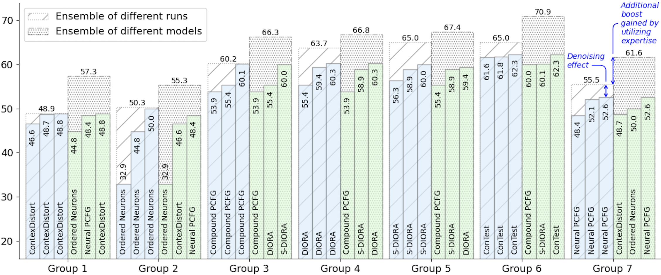
Figure 1: Effect of denoising vs. utilizing different expertise. Results are the $F_{1}$ scores on the PTB test set. The italic blue annotation is an interpretation of the plot.

Denoising vs. utilizing different expertise. A curious question raised from the main results is why our ensemble approach yields such a substantial improvement. We have two plausible hypotheses: 1) The ensemble approach merely smooths out the teachers’ noise, and 2) The ensemble approach is able to utilize different expertise of heterogeneous teachers.

We conducted the following experiment to verify the above hypotheses. Specifically, we compare two settings: the ensemble of three runs of the same model and the ensemble of three heterogeneous models. We picked the runs and models such that the two settings have similar performance. This sets up a controlled experiment, as the gain obtained by the ensemble of multiple runs suggests a denoising effect, whereas a further gain obtained by the ensemble of heterogeneous models suggests the effect of utilizing different expertise.

We repeated the experiment for seven groups with different choices of models and show results in Figure 1. As seen, the ensemble of different runs always outperforms a single run, showing that the denoising effect does play a role in the ensemble process. Moreover, the ensemble of heterogeneous models consistently leads to a large add-on improvement compared with the ensemble of multiple runs; the results convincingly verify that different unsupervised parsers learn different aspects of the language structures, and that our ensemble approach is able to utilize such different expertise.

Over-smoothing in multi-teacher knowledge distillation. As discussed in Section 2.4, union distillation is prone to the over-smoothing problem, where the student learns an overly smooth, wide-spreading distribution. This is especially severe in our setting, as our student learns from multiple heterogeneous teachers.

Distillation Approach	Mean Entropy	Std
Union distillation	11.42	0.10
Our ensemble distillation	4.93	0.13
Oracle-supervision distillation	2.26	0.13

Table 4: The mean and standard deviation (std) of the prediction entropy for distilled RNNGs.

The over-smoothing problem can be verified by checking the entropy, $-\sum_{x}p(x)\log p(x)$, of a model’s predicted distribution $p$. In Table 4, we report the mean and standard deviation of the entropy across five runs. Results clearly show that the union distillation leads to a very smooth distribution (very high entropy), which also explains its low

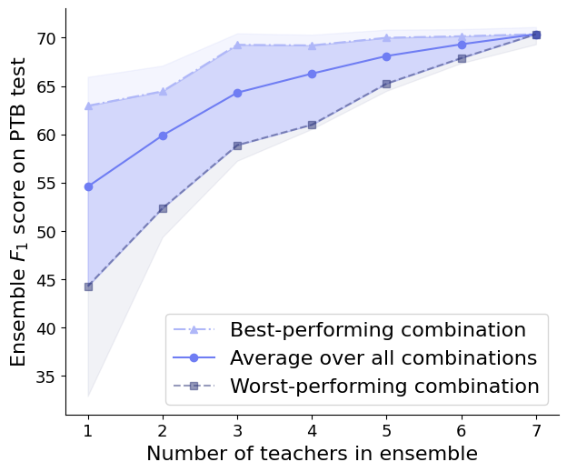
Figure 2: Ensemble performance with different numbers of teachers. The lines are best-performing, average, and worst-performing combinations. These results are averaged over five runs available in the experiments conducted for Table 2. The gray shades are the best and worst runs.

performance (Table 2). On the contrary, our ensemble-then-distill approach yields much lower entropy, providing strong evidence of the alleviation of the over-smoothing problem.

Analyzing the number of teachers. In our main experiment (Table 2), we perform an ensemble of seven popular unsupervised parsers. We would like to analyze the performance of ensemble models with different numbers of teachers, and results are shown in Figure 2.

We see a consistent trend that more teachers lead to higher performance. Profoundly, the top dashed line suggests that, even if we start with a strong teacher, adding weaker teachers also improves, or at least does not hurt, the performance. Further, the decrease in the width of gray shades (deviations of best and worst runs) suggests that more teachers also lead to lower variance. Overall, this analysis conclusively shows that, with a growing number of teachers, our ensemble approach not only improves performance, but also makes unsupervised parsing more robust.

Additional results. We present supplementary analyses in the appendix. B.1: Inference efficiency; B.2: Performance by different constituency types.

4 Related Work

Unsupervised syntactic structure discovery carries a long history and has attracted much attention in different ages (Klein, 2005; Shen et al., 2019; Li and Lu, 2023). Its significance lies in the potential to help low-resource domains (Kann et al., 2019) and its important role in cognitive science, such as understanding how children learn language (Bod, 2009). Peng et al. (2011) show unsupervised constituency parsing methods are not limited to linguistics but can also be used to parse motion-sensor data by treating it as a language. This approach finds an abstraction of motion data and leads to a better understanding of the signal semantics.

Unsupervised syntactic structure discovery can be divided into different tasks: unsupervised constituency parsing, which organizes the phrases of a sentence in a hierarchical manner (Carnie, 2007); unsupervised dependency parsing (Nivre, 2010; Naseem et al., 2010; Han et al., 2020), which determines the syntactic relation between the words in a sentence; and unsupervised chunking, which aims at segmenting a text into groups of syntactically related words in a flattened structure (Deshmukh et al., 2021; Wu et al., 2023).

Our work falls in the category of unsupervised constituency parsing. Previous work has proposed various heuristics and indirect supervisions to tackle this task (Snyder et al., 2009; Kim et al., 2019a; Drozdov et al., 2019), as mentioned in Section 1. In our work, we propose to build an ensemble model to utilize the expertise of different unsupervised parsers.

Minimum Bayes risk (MBR) decoding minimizes a Bayes risk (i.e., expected loss) during inference (Bickel and Doksum, 2015). For example, machine translation systems may generate a set of candidate outputs, and define the risk as the dissimilarity between one candidate output and the rest; MBR decoding selects the lowest-risk candidate translation that is most similar to others (Kumar and Byrne, 2004; Freitag et al., 2022; Suzgun et al., 2023). Similar approaches are applied to other decoding tasks, such as speech recognition (Gibson and Hain, 2006) and text summarization (Suzgun et al., 2023).

In this work, we develop a novel generative MBR method for constituency parsing that searches the entire binary tree space by an efficient CYK-like dynamic programming, significantly differing from existing MBR approaches that perform selection on a candidate set.

Knowledge distillation (KD) is commonly used to train a small student model from a large teacher model (Sun et al., 2019; Jiao et al., 2020). Evidence show that the teacher’s predicted probability contains more knowledge than a groundtruth label and can better train the student model (Hinton et al., 2015; Wen et al., 2023).

Interestingly, KD is originally proposed to train a small model from an ensemble of teachers (Buciluă et al., 2006; Hinton et al., 2015). They address simple classification tasks and use either voting or average ensembles to train the student. A voting ensemble is similar to MBR, but only works for classification tasks; it cannot be applied to structure prediction (e.g., sequences or trees). An average ensemble takes the average of probabilities; thus, it resembles union distillation, which is the predominant approach for multi-teacher distillation in recent years (Wu et al., 2021; Yang et al., 2020). However, these approaches may suffer from the over-smoothing problem when teachers are heterogeneous (Section 2.4). In our work, we propose a novel MBR-based ensemble method for multi-teacher distillation, which largely alleviates the over-smoothing problem and is able to utilize different teachers’ expertise.

5 Conclusion

In this work, we reveal an interesting phenomenon that different unsupervised parsers learn different expertise, and we propose a novel ensemble approach by introducing a new notion of “tree averaging” to leverage such heterogeneous expertise. Further, we distill the ensemble knowledge into a student model to improve inference efficiency; the proposed ensemble-then-distill approach also addresses the over-smoothing problem in multi-teacher distillation. Overall, our method shows consistent effectiveness with various teacher models and is robust in the domain-shift setting, largely bridging the gap between supervised and unsupervised constituency parsing.

Future work may be considered from both linguistic and machine learning perspectives. The proposed ensemble method largely bridges the gap between supervised and unsupervised parsing of the English language. A future direction is to address unsupervised linguistic structure discovery in low-resource and multilingual settings. Regarding the machine learning aspect, our work demonstrates the importance of addressing the over-smoothing problem in multi-teacher distillation, and we expect our ensemble-and-distill approach can be extended to different data types, such as sequences and graphs, with proper design of data-specific ensemble methods.

Appendix A Our CYK Variant

	Teacher 1									Teacher 2									Teacher 3									Teacher 4
Tree
						width("✧")
$\operatorname{HitCount}$					4
				1		1
			1		1		1
		3		0		3		1
	4		4		4		4		4
	$w_{1}$		$w_{2}$		$w_{3}$		$w_{4}$		$w_{5}$
	$b=1$									$b=2$									$b=3$									$b=4$
$l=2$
	$w_{1}$		$w_{2}$		$w_{3}$		$w_{4}$		$w_{5}$	$w_{1}$		$w_{2}$		$w_{3}$		$w_{4}$		$w_{5}$	$w_{1}$		$w_{2}$		$w_{3}$		$w_{4}$		$w_{5}$	$w_{1}$		$w_{2}$		$w_{3}$		$w_{4}$		$w_{5}$
$l=3$
	$w_{1}$		$w_{2}$		$w_{3}$		$w_{4}$		$w_{5}$	$w_{1}$		$w_{2}$		$w_{3}$		$w_{4}$		$w_{5}$	$w_{1}$		$w_{2}$		$w_{3}$		$w_{4}$		$w_{5}$
$l=4$
	$w_{1}$		$w_{2}$		$w_{3}$		$w_{4}$		$w_{5}$	$w_{1}$		$w_{2}$		$w_{3}$		$w_{4}$		$w_{5}$
$l=5$
	$w_{1}$		$w_{2}$		$w_{3}$		$w_{4}$		$w_{5}$

Figure 3: Step-by-step illustration of our CYK algorithm, showing the dynamic changes in the $H$ along with the construction of the corresponding optimal binary constituency tree.

In this appendix, we provide a step-by-step illustration of our CYK-based ensemble algorithm in Section 2.3.

Consider four teachers predicting the trees in the first row of Figure 3. The hit count of each span is shown in the second row. For example, the span $(w_{1}w_{2})$ hits $3$ times, namely, Teachers 1–3.

The initialization of the algorithm is to obtain the total hit count for a single word, which is simply the same as the number of teachers because every word appears intact in every teacher’s prediction. The initialization has five cells in a row, and is omitted in the figure to fit the page width.

For recursion, we first consider the constituents of two words, denoted by $l=2$. A constituent’s total hit count, denoted by $H_{b:e}$ in Eqn. (5), inherits those of its children, plus its own hit count. In the cell of $l=2,b=1$, for example, $H_{1:3}=4+4+3=11$, where $3$ is the hit count of the span $(w_{1}w_{2})$, shown before.

For the next step of recursion, we consider three-word constituents, i.e., $l=3$. For example, the span $w_{1}w_{2}w_{3}$ has two possible tree structures $(w_{1}(w_{2}w_{3}))$ and $((w_{1}w_{2})w_{3})$. The former leads to a total hit count of $13$, whereas the latter leads to $16$. Therefore, $((w_{1}w_{2})w_{3})$ highlighted in red is chosen, with the best hit count $H_{1:4}=16$.

The process is repeated until we have the best parse tree of the whole sentence, which is $l=5$ for the 5-word sentence in Figure 3. We also provide the pseudocode for the process in Algorithm 1.

Algorithm 1 Pseudocode for our CYK variant

1:function our_cyk($s,\{T_{i}\}_{i=1}^{K}$)

2:     for $b\leftarrow 1$ to $|s|$ do $\qquad\rhd$ Base cases

3:         $H_{b:b+1}=K$

4:         $L_{b:b+1}=\{s_{b:b+1}\}$

5:     end for

6:     for $l\leftarrow 2$ to $|s|$ do $\qquad\hskip 1.70709pt\rhd$Iterate over different lengths of constituents

7:         for $b\leftarrow 1$ to $|s|-l+1$ do $\qquad\rhd$ Iterate over different possible constituents of length $l$

8:              $e\leftarrow b+l$

9:              $j^{*}_{s:b}\leftarrow\operatorname*{arg\,max}\limits_{b<j<e}(H_{b:j}+H_{j:e}{\color[rgb]{.5,.5,.5}+\operatorname{HitCount}(s_{b:e},\{T_{i}(s)\}_{i=1}^{K})})$

10:                                   $\rhd$ The gray term need not be implemented as it is a constant in $j$

11:              $H_{b:e}\leftarrow H_{b:j^{*}_{s:b}}+H_{j^{*}_{s:b}:e}+\operatorname{HitCount}(s_{b:e},\{T_{i}(s)\}_{i=1}^{K})$

12:              $L_{b:e}\leftarrow L_{b:j^{*}_{s:b}}\cup L_{j^{*}_{s:b}:e}\cup\{s_{b:e}\}$

13:         end for

14:     end for

15:     return $L_{1:|s|+1}$

16:end function

Appendix B Supplementary Analyses

B.1 Inference Efficiency

		Inference Time (ms)
	Model	w/ GPU	w/o GPU
Teachers
	ON	35	130
	Neural PCFG	610	630
	Compound PCFG	560	590
	DIORA	30	30
	S-DIORA	110	140
	ConTest	4,300	59,500
	ContexDestort	1,890	11,110
Our ensemble
	CYK part	6	6
	Total	7,541	72,136
Student
	RNNG	410	410

Table 5: Per-sample inference time (in milliseconds) on the PTB test.

We propose to distill the ensemble knowledge into a student model to increase the inference efficiency. We conducted an analysis on the inference time of different approaches, where we measured the run time using 28 Intel(R) Core(TM) i9-9940X (@3.30GHz) CPUs with and without one Nvidia RTX Titan GPU. Table 5 reports the average time elapsed for performing inference on one sample of the PTB test set, ignoring loading models, reading inputs, and writing outputs.

In the table, the total inference time of our ensemble model is the summation of all the teachers and the CYK algorithm. As expected, an ensemble approach is slow because it has to perform inference for every teacher. However, our CYK-based ensemble algorithm is extremely efficient and its inference time is negligible compared with the teacher models.

The RNNG student model learns the knowledge from the cumbersome ensemble, and is able to perform inference efficiently with an 18x and 175x speedup with and without GPU, respectively. This shows the necessity of having knowledge distillation on top of the ensemble. Overall, RNNG achieves comparable performance to its ensemble teacher (Tables 2 and 3) but drastically speeds up the inference, being a useful model in practice.

B.2 Performance by Constituency Labels

In this work, we see different unsupervised parsers learn different patterns (Table 1), and their expertise can be utilized by an ensemble approach (Section 3.4). From the linguistic point of view, we are curious about whether there is a relation between such different expertise and the linguistic constituent labels (e.g., noun phrases and verb phrases).

With this motivation, we report in Figure 4 the breakdown performance by constituency labels, where the most common five labels—namely, noun phrases, propositional phrases, verb phrases, simple declarative clauses, and subordinating conjunction clauses—are considered, covering 95% of the cases in the PTB test. Notice that the predicted constituency parse trees are still unlabeled (without tags like noun phrases), whereas the groundtruth constituency labels are used for collecting the statistics. Consequently, only recall scores can be calculated in per-label performance analysis (Drozdov et al., 2019; Kim et al., 2019a; Cao et al., 2020).

As seen, existing unsupervised parsers indeed exhibit variations in the performance of different constituency labels. For example, ConTest achieves high performance of prepositional phrases, whereas DIORA works well for clauses (including simple declarative clauses and subordinating conjunction clauses); for noun phrases, most models perform similarly. By contrast, our ensemble model achieves outstanding performance similar to or higher than the best teacher in each category. This provides further evidence that our ensemble model utilizes different teachers’ expertise.

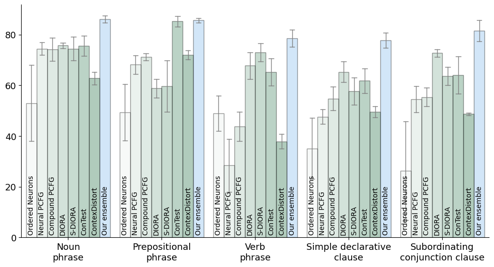
Figure 4: Performance by constituency labels on the PTB test set. Results are measured by recall, because the predicted parse trees are unlabeled; thus, precision and $F_{1}$ scores cannot be computed (Drozdov et al., 2019). Bars and gray intervals are the mean and standard deviation, respectively, over five runs.

Appendix C Inventory of Teacher Models

Our experiments involve seven existing unsupervised parsers as teachers, each of which has five runs either based on authors’ checkpoints or by our replication using authors’ codebases. We show the details in Table 6, where we also quote the mean $F_{1}$ scores and, if available, max $F_{1}$ scores reported in respective papers. Overall, we have achieved similar performance to previous work, which shows the success of our replication and establishes a solid foundation for our ensemble research.

	Run	Source	$F_{1}$
Ordered Neurons	mean $F_{1}=47.7$, max $F_{1}=49.4$ reported in Shen et al. (2019)
	1	Our replication using the original codebase ($\text{seed}=0017$)	$44.8$
	2	Our replication using the original codebase ($\text{seed}=0031$)	$32.9$
	3	Parsed data available in Kim et al. (2019a)	$50.0$
	4	Our replication using the original codebase ($\text{seed}=7214$)	$47.8$
	5	Our replication using the original codebase ($\text{seed}=1111$)	$45.9$
Neural PCFG	mean $F_{1}=50.8$, max $F_{1}=52.6$ reported in Kim et al. (2019a)
	1	Our replication using the original codebase ($\text{seed}=3435$)	$48.4$
	2	Parsed data available in the original codebase	$52.6$
	3	Our replication using the original codebase ($\text{seed}=1234$)	$52.1$
	4	Our replication using the original codebase ($\text{seed}=1313$)	$52.3$
	5	Our replication using the original codebase ($\text{seed}=5555$)	$49.8$
Compound PCFG	mean $F_{1}=50.8$, max $F_{1}=52.6$ reported in Kim et al. (2019a)
	1	Parsed data available in the original codebase	$60.1$
	2	Our replication using the original codebase ($\text{seed}=3435$)	$53.9$
	3	Our replication using the original codebase ($\text{seed}=1234$)	$55.4$
	4	Our replication using the original codebase ($\text{seed}=0887$)	$53.2$
	5	Our replication using the original codebase ($\text{seed}=0778$)	$55.0$
DIORA	mean $F_{1}=56.8$ reported in Drozdov et al. (2019)
	1	The mlp-softmax checkpoint available on the original codebase	$55.4$
	2	Our replication using the original codebase ($\text{seed}=0035$)	$59.4$
	3	Our replication using the original codebase ($\text{seed}=0074$)	$60.3$
	4	Our replication using the original codebase ($\text{seed}=1313$)	$60.5$
	5	Our replication using the original codebase ($\text{seed}=5555$)	$58.9$
S-DIORA	mean $F_{1}=57.6$, max $F_{1}=64.0$ reported in Drozdov et al. (2020)
	1	Our replication using the original codebase($\text{seed}=1943591871$)	$56.3$
	2	Our replication using the original codebase ($\text{seed}=0315$)	$60.9$
	3	Our replication using the original codebase ($\text{seed}=0075$)	$58.9$
	4	Our replication using the original codebase ($\text{seed}=1313$)	$54.7$
	5	Our replication using the original codebase ($\text{seed}=442597220$)	$54.9$
ConTest	mean $F_{1}=62.8$, max $F_{1}=65.9$ reported in Cao et al. (2020)
	1	A checkpoint provided by the authors through personal email	$65.9$
	2	Our replication using the original codebase ($\text{id}=0$)	$61.6$
	3	Parsed data provided by the authors through personal email	$62.3$
	4	Our replication using the original codebase ($\text{id}=1$)	$63.0$
	5	Our replication using the original codebase ($\text{id}=2$)	$61.8$
ContexDistort	$F_{1}=49.0$ reported in Li and Lu (2023)
	1	Our replication using the original codebase on 10th layer of “bert-base-cased”	$48.8$
	2	Our replication using the original codebase on 12th layer of “bert-base-cased”	$46.6$
	3	Our replication using the original codebase on 11th layer of “bert-base-cased”	$48.7$
	4	Our replication using the original codebase on 8th layer of “bert-base-cased”	$46.9$
	5	Our replication using the original codebase on 9th layer of “bert-base-cased”	$48.1$

Table 6: $F_{1}$ scores are on PTB test for different teachers in different runs. Note that the runs were randomly shuffled for the randomized experiment.

References

- Aho and Johnson (1974) Alfred V. Aho and Stephen C. Johnson. LR parsing. CSUR, 6(2):99–124, 1974.
- Bickel and Doksum (2015) Peter J Bickel and Kjell A Doksum. Mathematical Statistics: Basic Ideas and Selected Topics. CRC Press, 2015.
- Bod (2009) Rens Bod. From exemplar to grammar: A probabilistic analogy-based model of language learning. Cognitive Science, 33(5):752–793, 2009.
- Booth (1969) Taylor L. Booth. Probabilistic representation of formal languages. In Scandinavian Workshop on Algorithm Theory, 1969.
- Buciluă et al. (2006) Cristian Buciluă, Rich Caruana, and Alexandru Niculescu-Mizil. Model compression. In KDD, page 535–541, 2006.
- Cao et al. (2020) Steven Cao, Nikita Kitaev, and Dan Klein. Unsupervised parsing via constituency tests. In EMNLP, pages 4798–4808, 2020.
- Carnie (2007) Andrew Carnie. Syntax: A Generative Introduction. Blackwell Pub., 2 edition, 2007.
- Charniak (2000) Eugene Charniak. A maximum-entropy-inspired parser. In NAACL, pages 132–139, 2000.
- Clark (2001) Alexander Clark. Unsupervised induction of stochastic context-free grammars using distributional clustering. In CoNLL, 2001.
- Deshmukh et al. (2021) Anup Anand Deshmukh, Qianqiu Zhang, Ming Li, Jimmy Lin, and Lili Mou. Unsupervised chunking as syntactic structure induction with a knowledge-transfer approach. In Findings of EMNLP, pages 3626–3634, 2021.
- Devlin et al. (2019) Jacob Devlin, Ming-Wei Chang, Kenton Lee, and Kristina Toutanova. BERT: Pre-training of deep bidirectional transformers for language understanding. In NAACL-HLT, pages 4171–4186, 2019.
- Drozdov et al. (2019) Andrew Drozdov, Patrick Verga, Mohit Yadav, Mohit Iyyer, and Andrew McCallum. Unsupervised latent tree induction with deep inside-outside recursive auto-encoders. In NAACL-HLT, pages 1129–1141, 2019.
- Drozdov et al. (2020) Andrew Drozdov, Subendhu Rongali, Yi-Pei Chen, Tim O’Gorman, Mohit Iyyer, and Andrew McCallum. Unsupervised parsing with S-DIORA: Single tree encoding for deep inside-outside recursive autoencoders. In EMNLP, pages 4832–4845, 2020.
- Dyer et al. (2016) Chris Dyer, Adhiguna Kuncoro, Miguel Ballesteros, and Noah A. Smith. Recurrent neural network grammars. In NAACL-HLT, pages 199–209, 2016.
- Freitag et al. (2022) Markus Freitag, David Grangier, Qijun Tan, and Bowen Liang. High quality rather than high model probability: Minimum Bayes risk decoding with neural metrics. TACL, 10:811–825, 07 2022.
- Fromkin et al. (2003) Victoria Fromkin, Robert Rodman, and Nina Hyams. An Introduction to Language. Thomson/Heinle, 7 edition, 2003.
- Gibson and Hain (2006) Matthew Gibson and Thomas Hain. Hypothesis spaces for minimum Bayes risk training in large vocabulary speech recognition. In INTERSPEECH, pages 2406–2409, 2006.
- Han et al. (2020) Wenjuan Han, Yong Jiang, Hwee Tou Ng, and Kewei Tu. A survey of unsupervised dependency parsing. In COLING, pages 2522–2533, 2020.
- Hinton et al. (2015) Geoffrey Hinton, Oriol Vinyals, and Jeff Dean. Distilling the knowledge in a neural network. arXiv preprint arXiv:1503.02531, 2015.
- Jiao et al. (2020) Xiaoqi Jiao, Yichun Yin, Lifeng Shang, Xin Jiang, Xiao Chen, Linlin Li, Fang Wang, and Qun Liu. TinyBERT: Distilling BERT for natural language understanding. In Findings of EMNLP, pages 4163–4174, 2020.
- Kann et al. (2019) Katharina Kann, Anhad Mohananey, Samuel R. Bowman, and Kyunghyun Cho. Neural unsupervised parsing beyond English. In Proceedings of Workshop on Deep Learning for Low-Resource Natural Language Processing, pages 209–218, 2019.
- Kasami (1966) Tadao Kasami. An efficient recognition and syntax-analysis algorithm for context-free languages. Coordinated Science Laboratory Report, 1966.
- Kim et al. (2019a) Yoon Kim, Chris Dyer, and Alexander Rush. Compound probabilistic context-free grammars for grammar induction. In ACL, pages 2369–2385, 2019a.
- Kim et al. (2019b) Yoon Kim, Alexander Rush, Lei Yu, Adhiguna Kuncoro, Chris Dyer, and Gábor Melis. Unsupervised recurrent neural network grammars. In NAACL-HLT, pages 1105–1117, 2019b.
- Klein (2005) Dan Klein. The Unsupervised Learning of Natural Language Structure. Stanford University, 2005.
- Klein and Manning (2002) Dan Klein and Christopher D. Manning. A generative constituent-context model for improved grammar induction. In ACL, pages 128–135, 2002.
- Kumar and Byrne (2004) Shankar Kumar and William Byrne. Minimum Bayes-risk decoding for statistical machine translation. In HLT-NAACL, pages 169–176, 2004.
- Li et al. (2019) Bowen Li, Lili Mou, and Frank Keller. An imitation learning approach to unsupervised parsing. In ACL, pages 3485–3492, 2019.
- Li and Lu (2023) Jiaxi Li and Wei Lu. Contextual distortion reveals constituency: Masked language models are implicit parsers. In ACL, pages 5208–5222, 2023.
- Manacher (1978) Glenn K. Manacher. An improved version of the Cocke-Younger-Kasami algorithm. Computer Languages, 3(2):127–133, 1978.
- Marcus et al. (1993) Mitchell P. Marcus, Beatrice Santorini, and Mary Ann Marcinkiewicz. Building a large annotated corpus of English: The Penn Treebank. Computational Linguistics, 19(2):313–330, 1993.
- Maveli and Cohen (2022) Nickil Maveli and Shay Cohen. Co-training an unsupervised constituency parser with weak supervision. In Findings of ACL, pages 1274–1291, 2022.
- McCawley (1998) James D. McCawley. The Syntactic Phenomena of English. University of Chicago Press, 1998.
- Mohammadshahi and Henderson (2023) Alireza Mohammadshahi and James Henderson. Syntax-aware graph-to-graph transformer for semantic role labelling. In RepL4NLP, pages 174–186, 2023.
- Naseem et al. (2010) Tahira Naseem, Harr Chen, Regina Barzilay, and Mark Johnson. Using universal linguistic knowledge to guide grammar induction. In EMNLP, pages 1234–1244, 2010.
- Nivre (2010) Joakim Nivre. Dependency parsing. Language and Linguistics Compass, 4(3):138–152, 2010.
- Peng et al. (2011) Huan-Kai Peng, Pang Wu, Jiang Zhu, and Joy Ying Zhang. Helix: Unsupervised grammar induction for structured activity recognition. In ICDM, pages 1194–1199, 2011.
- Sampson (2002) Geoffrey Sampson. English for the computer: The SUSANNE corpus and analytic scheme. Computational Linguistics, 28(1):102–103, 2002.
- Sennrich (2014) Rico Sennrich. A CYK+ variant for SCFG decoding without a dot chart. In Proceedings of the Workshop on Syntax, Semantics and Structure in Statistical Translation, pages 94–102, 2014.
- Shen et al. (2018) Yikang Shen, Zhouhan Lin, Chin-Wei Huang, and Aaron Courville. Neural language modeling by jointly learning syntax and lexicon. In ICLR, 2018.
- Shen et al. (2019) Yikang Shen, Shawn Tan, Alessandro Sordoni, and Aaron Courville. Ordered neurons: Integrating tree structures into recurrent neural networks. In ICLR, 2019.
- Snyder et al. (2009) Benjamin Snyder, Tahira Naseem, and Regina Barzilay. Unsupervised multilingual grammar induction. In ACL, pages 73–81, 2009.
- Sun et al. (2019) Siqi Sun, Yu Cheng, Zhe Gan, and Jingjing Liu. Patient knowledge distillation for BERT model compression. In EMNLP-IJCNLP, pages 4323–4332, 2019.
- Suzgun et al. (2023) Mirac Suzgun, Luke Melas-Kyriazi, and Dan Jurafsky. Follow the wisdom of the crowd: Effective text generation via minimum Bayes risk decoding. In Findings of ACL, pages 4265–4293, 2023.
- Tenney et al. (2019) Ian Tenney, Dipanjan Das, and Ellie Pavlick. BERT rediscovers the classical NLP pipeline. In ACL, pages 4593–4601, 2019.
- Wei et al. (2019) Bolin Wei, Shuai Lu, Lili Mou, Hao Zhou, Pascal Poupart, Ge Li, and Zhi Jin. Why do neural dialog systems generate short and meaningless replies? A comparison between dialog and translation. In ICASSP, pages 7290–7294, 2019.
- Wen et al. (2022) Yuqiao Wen, Yongchang Hao, Yanshuai Cao, and Lili Mou. An equal-size hard EM algorithm for diverse dialogue generation. In ICLR, 2022.
- Wen et al. (2023) Yuqiao Wen, Zichao Li, Wenyu Du, and Lili Mou. -divergence minimization for sequence-level knowledge distillation. In ACL, pages 10817–10834, 2023.
- Wu et al. (2021) Chuhan Wu, Fangzhao Wu, and Yongfeng Huang. One teacher is enough? Pre-trained language model distillation from multiple teachers. In Findings of ACL-IJCNLP, pages 4408–4413, 2021.
- Wu et al. (2023) Zijun Wu, Anup Anand Deshmukh, Yongkang Wu, Jimmy Lin, and Lili Mou. Unsupervised chunking with hierarchical RNN. arXiv preprint arXiv:2309.04919, 2023.
- Yang et al. (2020) Ze Yang, Linjun Shou, Ming Gong, Wutao Lin, and Daxin Jiang. Model compression with two-stage multi-teacher knowledge distillation for web question answering system. In WSDM, pages 690–698, 2020.
- Younger (1967) Daniel H. Younger. Recognition and parsing of context-free languages in time . Information and Control, 10(2):189–208, 1967.
- Zhang et al. (2021) Yu Zhang, Houquan Zhou, and Zhenghua Li. Fast and accurate neural CRF constituency parsing. In IJCAI, pages 4046–4053, 2021.