Greedy invariant-domain preserving approximation for hyperbolic systems

Abstract

The paper focuses on invariant-domain preserving approximations of hyperbolic systems. We propose a new way to estimate the artificial viscosity that has to be added to make explicit, conservative, consistent numerical methods invariant-domain preserving and entropy inequality compliant. Instead of computing an upper bound on the maximum wave speed in Riemann problems, we estimate a minimum wave speed in the said Riemann problems such that the approximation satisfies predefined invariant-domain properties and predefined entropy inequalities. This technique eliminates non-essential fast waves from the construction of the artificial viscosity, while preserving pre-assigned invariant-domain properties and entropy inequalities.

35L65, 65M60, 65M12, 65N30

1 Introduction

Let us consider the hyperbolic system of conservation equations $\partial_{t}{\bm{u}}+\nabla{\cdot}{\mathbbm{f}}({\bm{u}})={\bm{0}}$, where ${\bm{u}}$ denotes a conserved state taking values in ${\mathbb{R}}^{m}$ and ${\mathbbm{f}}({\bm{u}})$ an associated flux taking values in ${\mathbb{R}}^{m{\times}d}$, where $d$ is the space dimension. Most explicit approximation methods for solving this type of system are based on some notion of numerical flux and involve some numerical dissipation. For instance, all the methods based on Lax’s seminal paper [15, p. 163] involve numerical fluxes between pairs of degrees of freedom, say $i,j$, that take the following form $\frac{1}{2}({\mathbbm{f}}(\textsf{{U}}_{i})+{\mathbbm{f}}(\textsf{{U}}_{j})){\bm{n}}_{ij}+\alpha_{ij}(\textsf{{U}}_{i}-\textsf{{U}}_{j})$, where ${\bm{n}}_{ij}$ is some unit vector associated with the space discretization at hand and $\alpha_{ij}$ is an upper bound on the maximum wave speed in the Riemann problem using the flux ${\mathbbm{f}}(\textsf{{U}}){\bm{n}}_{ij}$ and the states $\textsf{{U}}_{i}$ and $\textsf{{U}}_{j}$ as left and right Riemann data. Denoting by $\lambda_{\max}({\bm{n}}_{ij},\textsf{{U}}_{i},\textsf{{U}}_{j})$ the maximum wave speed in the Riemann problem in question, it is now well established that choosing $\alpha_{ij}$ such that $\alpha_{ij}\geq\lambda_{\max}({\bm{n}}_{ij},\textsf{{U}}_{i},\textsf{{U}}_{j})$ guarantees that some invariant-domain property can be extracted from the scheme; see e.g., Harten et al. [10], Tadmor [23, p. 375], Perthame and Shu [20, §5]. Using $\lambda_{\max}({\bm{n}}_{ij},\textsf{{U}}_{i},\textsf{{U}}_{j})$ to construct invariant-domain preserving schemes dates back to the origins of computational fluid dynamics; we refer the reader for instance to [15, p. 163]. Recalling that the flux $\alpha_{ij}(\textsf{{U}}_{i}-\textsf{{U}}_{j})$ is associated with numerical dissipation and therefore induces a loss of accuracy, a natural question to ask is whether it is possible to estimate a greedy value for $\alpha_{ij}$ in the open interval $(0,\lambda_{\max}({\bm{n}}_{ij},\textsf{{U}}_{i},\textsf{{U}}_{j}))$ guaranteeing that the scheme satisfies the desired invariant-domain properties and relevant entropy inequalities. It is the purpose of the present paper to give a positive answer to this question. The paper is the result of a research project that was initiated at the 9th International Conference on Numerical Methods for Multi-Material Fluid Flow, held in Trento, Italy, 9-13, September 2019. Some of the questions posed above and some answers thereto were outlined in [8].

To convince the reader that the program described above is feasible, let us consider the compressible Euler equations equipped with a $\gamma$-law, and let us consider the Riemann problem with the flux ${\mathbbm{f}}({\bm{u}}){\cdot}{\bm{n}}$ and some left and right data ${\bm{u}}_{L},{\bm{u}}_{R}$. Then denoting by $\lambda_{1}^{-},\lambda_{1}^{+}$ the two wave speeds enclosing the $1$-wave, $\lambda_{2}$ the speed of the $2$-wave (i.e., the contact discontinuity), and $\lambda_{3}^{-},\lambda_{3}^{+}$ the two wave speeds enclosing the $3$-wave, we have $\lambda_{1}^{-}\leq\lambda_{1}^{+}\leq\lambda_{2}\leq\lambda_{3}^{-}\leq\lambda_{3}^{+}$, and the maximum wave speed in the Riemann problem is $\lambda_{\max}({\bm{n}},{\bm{u}}_{L},{\bm{u}}_{R}):=\max(|\lambda_{1}^{-}|,|\lambda_{3}^{+}|)>|\lambda_{2}|$. If the Riemann data yields a solution that consists of just one contact discontinuity, one can establish that the amount of viscosity that is sufficient to satisfy all the invariant domain properties (in addition to local entropy inequalities) is just $|\lambda_{2}|$ (because the velocity and the pressure are constant in this case). Hence setting the graph viscosity wave speed $\alpha$ to be larger than or equal to $\lambda_{\max}({\bm{n}},{\bm{u}}_{L},{\bm{u}}_{R})$ is needlessly over-diffusive since taking $\alpha=|\lambda_{2}|$ is sufficient in this case. Invoking the continuous dependence of the Riemann solution with respect to the data, one then realizes that a similar conclusion holds if the Riemann data is a small perturbation of a data set producing a contact discontinuity only. The situation described above is well illustrated by the multi-material Euler equations in Lagrangian coordinates. In this case the interface between two materials is a contact discontinuity that should keep its integrity over time. Let $v:={\bm{u}}{\cdot}{\bm{n}}$ denote the component of the material velocity normal to the interface. The maximum wave speed in the Riemann problem using the two states on either sides of the interface gives $\lambda_{\max}({\bm{n}},{\bm{u}}_{L},{\bm{u}}_{R})=\max(|\lambda_{1}^{-}-v|,|\lambda_{3}^{+}-v|)$ in the Lagrangian reference frame, whereas the wave speed of the $2$-wave is $\lambda_{2}-v=0$. In this case the amount of viscosity that is sufficient to satisfy all the invariant domain properties is $\alpha=\lambda_{2}-v=0$. Hence, if one instead uses $\alpha=\lambda_{\max}:=\max(|\lambda_{1}^{-}-v|,|\lambda_{3}^{+}-v|)$ (as suggested e.g., in Guermond et al. [5] and most of the literature on the topic) one needlessly diffuses the contact discontinuity. The purpose of the present paper is to clarify the issues described above and derive a variation of the method presented in [2, 5] that is invariant-domain preserving, satisfies discrete entropy inequalities, and minimizes the amount of artificial viscosity used.

The paper is organized as follows. We formulate the problem and recall important concepts that are used in the paper in §2. We introduce in §3 the concept of greedy viscosity for any hyperbolic system. The key results of this section are the definitions (3.7) and (3.8) and Theorem 3.8. The concept of greedy viscosity is then illustrated for scalar conservation equations in §4. The main result summarizing the content of this section are the definitions (4.2), (4.3) and Theorem 4.5. (Due to lack of space, the concept of greedy viscosity for systems like the compressible Euler equation equipped with a tabulated equation of state will be illustrated in the forthcoming second part of this work.) The ideas introduced in the paper are numerically illustrated in §6 for scalar conservation equations and for the $p$-system. Some of these tests are meant to illustrate that estimating a greedy wave speed in order to preserve the invariant-domain is not sufficient to converge to an entropy solution. Ensuring that entropy inequalities are satisfied is essential for this matter. We also show that using just one entropy is not sufficient for scalar conservation equations with a non-convex flux.

2 Formulation of the problem

In this section we formulate the question that is addressed in the paper and put it in context.

2.1 The hyperbolic system

Our objective is to develop elementary and robust numerical tools to approximate hyperbolic systems in conservation form:

(2.1) $$\begin{cases}\partial_{t}{\bm{u}}+\nabla{\cdot}{\mathbbm{f}}({\bm{u}})={\bm{0}},\quad\mbox{for}\,({\bm{x}},t)\in D{\times}{\mathbb{R}}_{+},\\ {\bm{u}}({\bm{x}},0)={\bm{u}}_{0}({\bm{x}}),\quad\mbox{for}\,{\bm{x}}\in{\mathbb{R}}^{d}.\end{cases}$$

Here $d$ is the space dimension, $D$ is a compact, connected, polygonal subset of ${\mathbb{R}}^{d}$. To avoid difficulties related to boundary conditions, we either solve the Cauchy problem or assume that the boundary conditions are periodic. The dependent variable (or state variable) ${\bm{u}}$ takes values in ${\mathbb{R}}^{m}$. The function ${\mathbbm{f}}:{\mathcal{A}}\to({\mathbb{R}}^{m})^{d}$ is called flux. The domain of ${\mathbbm{f}}$, i.e., ${\mathcal{A}}\subset{\mathbb{R}}^{m}$, is called admissible set. The state variable ${\bm{u}}$ is viewed as a column vector ${\bm{u}}=(u_{1},\ldots,u_{m})^{\mathsf{T}}$. The flux is a $m{\times}d$ matrix with entries ${\mathbbm{f}}_{ik}({\bm{u}}({\bm{x}}))$, $i\in\{1\hskip 0.50003pt{:}\hskip 1.00006ptm\}$, $k\in\{1\hskip 0.50003pt{:}\hskip 1.00006ptd\}$ and $\nabla{\cdot}{\mathbbm{f}}({\bm{u}}({\bm{x}}))$ is a column vector with entries $(\nabla{\cdot}{\mathbbm{f}}({\bm{u}}))_{i}=\sum_{k\in\{1\hskip 0.35002pt{:}\hskip 0.70004ptd\}}\partial_{x_{k}}{\mathbbm{f}}_{ik}({\bm{u}}({\bm{x}}))$. For any ${\bm{n}}=(n_{1}\ldots,n_{d})^{\mathsf{T}}\in{\mathbb{R}}^{d}$, we denote ${\mathbbm{f}}({\bm{u}}){\bm{n}}$ the column vector with entries $\sum_{l\in\{1\hskip 0.35002pt{:}\hskip 0.70004ptd\}}{\mathbbm{f}}_{il}({\bm{u}})n_{l}$, where $i\in\{1\hskip 0.50003pt{:}\hskip 1.00006ptm\}$.

We assume in the entire paper that the admissible set ${\mathcal{A}}\subset{\mathbb{R}}^{m}$ is constructed such that for every pair of states $({\bm{u}}_{L},{\bm{u}}_{R})\in{\mathcal{A}}{\times}{\mathcal{A}}$ and every unit vector ${\bm{n}}$ in ${\mathbb{R}}^{d}$, the following one-dimensional Riemann problem

(2.2) $$\partial_{t}{\bm{w}}+\partial_{x}({\mathbbm{f}}({\bm{w}}){\bm{n}})=0,\quad(x,t)\in{\mathbb{R}}{\times}{\mathbb{R}}_{+},\qquad{\bm{w}}(x,0)=\begin{cases}{\bm{u}}_{L},&\text{if $x<0$}\\ {\bm{u}}_{R},&\text{if $x>0$},\end{cases}$$

has a unique solution satisfying adequate entropy inequalities. We assume that this solution is self-similar with self-similarity parameter $\xi{:=}\frac{x}{t}$, and we set

(2.3) $${\bm{v}}({\bm{n}},{\bm{u}}_{L},{\bm{u}}_{R},\frac{x}{t}){:=}{\bm{w}}(x,t);$$

see for instance Lax [16], Toro [24]. Using Lax’s notation, we denote by $\lambda_{1}^{-}\leq\lambda_{1}^{+}$ the two wave speeds enclosing the $1$-wave (i.e., the leftmost wave) and $\lambda_{m}^{-}\leq\lambda_{m}^{+}$ the two wave speeds enclosing the $m$-wave (i.e., the rightmost wave). The key result that we are going to use in the paper is that ${\bm{v}}({\bm{n}},{\bm{u}}_{L},{\bm{u}}_{R},\xi)={\bm{u}}_{L}$ if $\xi\leq\lambda_{1}^{-}$ and ${\bm{v}}({\bm{n}},{\bm{u}}_{L},{\bm{u}}_{R},\xi)={\bm{u}}_{R}$ if $\xi\geq\lambda_{m}^{+}$. We define a left wave speed $\lambda_{L}({\bm{n}},{\bm{u}}_{L},{\bm{u}}_{R}){:=}\lambda_{1}^{-}$ and a right wave speed $\lambda_{R}({\bm{n}},{\bm{u}}_{L},{\bm{u}}_{R}){:=}\lambda_{m}^{+}$. We also define the maximum wave speed of the Riemann problem to be

(2.4) $$\lambda_{\max}({\bm{n}},{\bm{u}}_{L},{\bm{u}}_{R}){:=}\max(|\lambda_{L}({\bm{n}},{\bm{u}}_{L},{\bm{u}}_{R})|,|\lambda_{R}({\bm{n}},{\bm{u}}_{L},{\bm{u}}_{R})|).$$

We will replace the notation $\lambda_{\max}({\bm{n}},{\bm{u}}_{L},{\bm{u}}_{R})$ by $\lambda_{\max}$ when the context is unambiguous. For further reference, for every $t>0$ we define

(2.5) $$\overline{\bm{v}}(t,{\bm{n}},{\bm{u}}_{L},{\bm{u}}_{R}):=\int_{-\frac{1}{2}}^{\frac{1}{2}}{\bm{v}}({\bm{n}},{\bm{u}}_{L},{\bm{u}}_{R},\tfrac{x}{t})\,{\mathrm{d}}x.$$

Notice that if $t\lambda_{\max}({\bm{n}},{\bm{u}}_{L},{\bm{u}}_{R})\leq\frac{1}{2}$, then $\overline{\bm{v}}(t,{\bm{n}},{\bm{u}}_{L},{\bm{u}}_{R})$ is the average of the entropy solution of the Riemann problem (2.2) over the Riemann fan. This property is illustrated in Figure 1.

Figure 1: Riemann problem and Riemann fan.

Definition 2.1 (Invariant domain).

We say that ${\mathcal{B}}\subset{\mathcal{A}}\subset{\mathbb{R}}^{m}$ is invariant domain for (2.1) if the following holds true: (i) ${\mathcal{B}}$ is convex; (ii) for any pair $({\bm{u}}_{L},{\bm{u}}_{R})\in{\mathcal{B}}{\times}{\mathcal{B}}$, any unit vector ${\bm{n}}\in{\mathbb{R}}^{d}$, and all $t\in\big{(}0,\frac{1}{2\lambda_{\max}({\bm{n}},{\bm{u}}_{L},{\bm{u}}_{R})}\big{)}$, we have $\overline{\bm{v}}(t,{\bm{n}},{\bm{u}}_{L},{\bm{u}}_{R})\in{\mathcal{B}}$, where $\overline{\bm{v}}$ is given by (2.5). $\square$

Lemma 2.2 (Invariance of the auxiliary states).

Let ${\mathcal{B}}\subset{\mathcal{A}}$ be any invariant domain for (2.1). Let $(\eta,{\bm{q}})$ be an entropy pair for (2.1). Let $\lambda>0$, let ${\bm{n}}\in{\mathbb{R}}^{d}$ be a unit vector. For all ${\bm{u}}_{L}$, ${\bm{u}}_{R}$ in ${\mathcal{A}}$, consider the following auxiliary state:

(2.6) $$\overline{{\bm{u}}}_{LR}(\lambda):=\frac{1}{2}({\bm{u}}_{L}+{\bm{u}}_{R})-\frac{1}{2\lambda}\left({\mathbbm{f}}({\bm{u}}_{R})-{\mathbbm{f}}({\bm{u}}_{L})\right){\bm{n}}.$$

Assume that ${\bm{u}}_{L},{\bm{u}}_{R}\in{\mathcal{B}}$, and $\lambda\geq\lambda_{\max}({\bm{n}},{\bm{u}}_{L},{\bm{u}}_{R})$. Then

(2.7) $$\overline{{\bm{u}}}_{LR}(\lambda)=\overline{\bm{v}}\left(\tfrac{1}{2\lambda},{\bm{n}},{\bm{u}}_{L},{\bm{u}}_{R}\right),$$

(2.8) $$\overline{{\bm{u}}}_{LR}(\lambda)\in{\mathcal{B}},$$

(2.9) $$\eta(\overline{\bm{u}}_{LR}(\lambda))\leq\tfrac{1}{2}(\eta({\bm{u}}_{L})+\eta({\bm{u}}_{R}))-\tfrac{1}{2\lambda}\left({\bm{q}}({\bm{u}}_{R})-{\bm{q}}({\bm{u}}_{L})\right){\cdot}{\bm{n}}$$

$\square$

Proof 2.3.

See e.g., Lemma 2.1 and Lemma 2.2 in [2]. $\square$

2.2 Agnostic space approximation

Without going into details, we now assume that we have at hand a fully discrete scheme where time is approximated by using the forward Euler time stepping and space is approximated by using some “centered” approximation of (2.1), i.e., without any artificial viscosity to stabilize the approximation. We denote by $t^{n}$ the current time, $n\in{\mathbb{N}}$, and we denote by ${\tau}$ the current time step size; that is $t^{n+1}:=t^{n}+{\tau}$ (we should write ${\tau}^{n}$ as the time step may vary at each time step, but we omit the super-index ⁿ to simplify the notation). Let us assume that the current approximation is a collection of states $\{\textsf{{U}}_{i}^{n}\}_{i\in{\mathcal{V}}}$, where the index set ${\mathcal{V}}$ is used to enumerate all the degrees of freedom of the approximation. We assume that the “centered” update is given by $\textsf{{U}}_{i}^{\textup{G},n+1}$ with

(2.10) $$\frac{m_{i}}{{\tau}}(\textsf{{U}}_{i}^{\textup{G},n+1}-\textsf{{U}}_{i}^{n})+\!\!\sum_{j\in{\mathcal{I}}(i)}{\mathbbm{f}}(\textsf{{U}}_{j}^{n}){\bm{c}}_{ij}={\bm{0}}.$$

The quantity $m_{i}$ is called lumped mass and we assume that $m_{i}>0$ for all $i\in{\mathcal{V}}$. The index set ${\mathcal{I}}(i)$ is called local stencil. This set collects only the degrees of freedom in ${\mathcal{V}}$ that interact with $i$. We set ${\mathcal{I}}(i)^{*}{:=}{\mathcal{I}}(i){\setminus}\{i\}$. The vector ${\bm{c}}_{ij}\in{\mathbb{R}}^{d}$ encodes the space discretization. We view $\frac{1}{m_{i}}\sum_{j\in{\mathcal{I}}(i)}{\mathbbm{f}}(\textsf{{U}}_{j}^{n}){\bm{c}}_{ij}$ as a Galerkin (or centered or inviscid) approximation of $\nabla{\cdot}{\mathbbm{f}}({\bm{u}})$ at time $t^{n}$ at some grid point (or cell) $i\in{\mathcal{V}}$. The superscript ${}^{\textup{G}}$ is meant to remind us that (2.10) is a Galerkin (or inviscid or centered) approximation of (2.1). That is, we assume that the consistency error in space in (2.10) scales optimally with respect to the mesh size for the considered approximation setting. We keep the discussion at this abstract level for the sake of generality; see Remark 2.4. The only requirement that we make on the coefficients ${\bm{c}}_{ij}$ is that the method is conservative; that is to say, we assume that

(2.11) $${\bm{c}}_{ij}=-{\bm{c}}_{ji}\quad\text{and}\quad\sum_{j\in{\mathcal{I}}(i)}{\bm{c}}_{ij}={\bm{0}}.$$

An immediate consequence of this assumption is that the total mass is conserved: $\sum_{i\in{\mathcal{V}}}m_{i}\textsf{{U}}_{i}^{\textup{G},n+1}=\sum_{i\in{\mathcal{V}}}m_{i}\textsf{{U}}_{i}^{n}$.

Of course, (2.10) is in general not appropriate if the solution to (2.1) is not smooth. To recover some sort of stability (the exact notion of stability we have in mind is defined in Theorem 2.5) we modify the scheme by adding a graph viscosity based on the stencil ${\mathcal{I}}(i)$; that is, we compute the stabilized update $\textsf{{U}}_{i}^{n+1}$ by setting:

(2.12) $$\frac{m_{i}}{{\tau}}(\textsf{{U}}_{i}^{n+1}-\textsf{{U}}_{i}^{n})+\!\!\sum_{j\in{\mathcal{I}}(i)}{\mathbbm{f}}(\textsf{{U}}_{j}^{n}){\bm{c}}_{ij}-\!\!\sum_{j\in{\mathcal{I}}(i)^{*}}d_{ij}^{n}(\textsf{{U}}^{n}_{j}-\textsf{{U}}^{n}_{i})={\bm{0}}.$$

Here $d_{ij}^{n}$ is the yet to be defined graph viscosity. We assume that

(2.13) $$d_{ij}^{n}=d_{ji}^{n}>0,\quad\text{if}\quad i\neq j.$$

The symmetry implies that the method remains conservative. The question addressed in the paper is the following: how large has $d_{ij}^{n}$ to be chosen so that (2.12) preserves invariant domains and satisfies entropy inequalities (for some finite collection of entropies)?

Remark 2.4 (Literature).

The algorithm (2.12) is a generalization of [15, p. 163]; see also Harten et al. [10], Tadmor [23, p. 375], Perthame and Shu [20, §5] and the literature cited in these references. The reader is referred to [2], [6] for realizations of the above algorithm with continuous finite elements. Realizations of the algorithm with discontinuous elements and with finite volumes are described in [7]. $\square$

2.3 The auxiliary bar states

We now recall the main stability result established in [2]. The proof of this result is the source of inspiration for the rest of the paper. For all $i\in{\mathcal{V}}$ and all $j\in{\mathcal{I}}(i)$ we introduce the unit vector ${\bm{n}}_{ij}:={\bm{c}}_{ij}/\|{\bm{c}}_{ij}\|_{\ell^{2}}$. Given two states $\textsf{{U}}_{i}^{n}$ and $\textsf{{U}}_{j}^{n}$ in ${\mathcal{A}}$, we recall that $\lambda_{\max}({\bm{n}}_{ij},\textsf{{U}}_{i}^{n},\textsf{{U}}_{j}^{n})$ is the maximum wave speed in the Riemann problem defined in §2.1 with left state $\textsf{{U}}_{i}^{n}$, right state $\textsf{{U}}_{j}^{n}$, and unit vector ${\bm{n}}_{ij}$. The guaranteed maximum speed (GMS) graph viscosity $d_{ij}^{\textup{\tiny GMS},n}$ is defined in [2] as follows:

(2.14) $$d_{ij}^{\textup{\tiny GMS},n}:=\max\big{(}\lambda_{\max}({\bm{n}}_{ij},\textsf{{U}}_{i}^{n},\textsf{{U}}_{j}^{n})\|{\bm{c}}_{ij}\|_{\ell^{2}},\lambda_{\max}({\bm{n}}_{ji},\textsf{{U}}_{j}^{n},\textsf{{U}}_{i}^{n})\|{\bm{c}}_{ji}\|_{\ell^{2}}\big{)}.$$

Theorem 2.5 (Local invariance).

Let ${\mathcal{B}}\subset{\mathcal{A}}$ be any invariant domain for (2.1). Let $(\eta,{\bm{q}})$ be any entropy pair for (2.1). Let $n\geq 0$ and $i\in{\mathcal{V}}$. Let $d_{ij}^{n}$ be any graph viscosity such that $d_{ij}^{n}\geq d_{ij}^{\textup{\tiny GMS},n}$ and $d_{ij}^{n}>0$. Assume that $0<{\tau}\leq m_{i}/\sum_{j\in{\mathcal{I}}(i)^{*}}2d_{ij}^{n}$. Assume that $\{\textsf{{U}}_{j}^{n}\}_{j\in{\mathcal{I}}(i)}\subset{\mathcal{B}}$. Then the update $\{\textsf{{U}}_{i}^{n+1}\}_{i\in{\mathcal{V}}}$ given by (2.12) satisfies the following properties:

(2.15) $$\textsf{{U}}_{i}^{n+1}\in{\mathcal{B}},$$

(2.16) $$\frac{m_{i}}{{\tau}}(\eta(\textsf{{U}}_{i}^{n+1})-\eta(\textsf{{U}}_{i}^{n}))+\sum_{j\in{\mathcal{I}}(i)}{\bm{c}}_{ij}{\cdot}{\bm{q}}(\textsf{{U}}_{j}^{n})-\!\!\!\sum_{j\in{\mathcal{I}}(i)^{*}}\!\!\!d_{ij}^{n}(\eta(\textsf{{U}}_{j}^{n})-\eta(\textsf{{U}}_{j}^{n}))\leq 0.$$

$\square$

Proof 2.6.

We refer to Theorem 4.1 and Theorem 4.5 in [2] for detailed proofs. But since these proofs contain ideas that are going to be used latter in the paper, we now reproduce the key arguments. Using the conservation property (2.11), i.e., $\sum_{j\in{\mathcal{I}}(i)}{\bm{c}}_{ij}={\bm{0}}$, we rewrite (2.12) as follows:

$$\frac{m_{i}}{{\tau}}(\textsf{{U}}_{i}^{n+1}-\textsf{{U}}_{i}^{n})+\!\!\sum_{j\in{\mathcal{I}}(i)^{*}}\Big{(}2d_{ij}^{n}\textsf{{U}}^{n}_{i}+({\mathbbm{f}}(\textsf{{U}}_{j}^{n})-{\mathbbm{f}}(\textsf{{U}}_{i}^{n})){\bm{c}}_{ij}-d_{ij}^{n}(\textsf{{U}}^{n}_{j}+\textsf{{U}}^{n}_{i})\Big{)}={\bm{0}}.$$

Then, recalling that $d_{ij}^{n}>0$ by assumption, we introduce the auxiliary states

(2.17) $$\overline{\textsf{{U}}}_{ij}^{n}:=\frac{1}{2}(\textsf{{U}}^{n}_{i}+\textsf{{U}}^{n}_{j})-({\mathbbm{f}}(\textsf{{U}}_{j}^{n})-{\mathbbm{f}}(\textsf{{U}}_{i}^{n})){\bm{n}}_{ij}\frac{\|{\bm{c}}_{ij}\|_{\ell^{2}}}{2d_{ij}^{n}}.$$

This allows us to rewrite (2.12) as follows:

(2.18) $$\textsf{{U}}_{i}^{n+1}=\bigg{(}1-\!\!\sum_{j\in{\mathcal{I}}(i)^{*}}\frac{2{\tau}d_{ij}^{n}}{m_{i}}\bigg{)}\textsf{{U}}_{i}^{n}+\!\!\sum_{j\in{\mathcal{I}}(i)^{*}}\frac{2{\tau}d_{ij}^{n}}{m_{i}}\overline{\textsf{{U}}}_{ij}^{n}.$$

Since we assumed that $1-2\frac{{\tau}}{m_{i}}\sum_{j\in{\mathcal{I}}(i)^{*}}d_{ij}^{n}>0$, the right-hand side in the above identity is a convex combination of the states $\{\overline{\textsf{{U}}}_{ij}^{n}\}_{j\in{\mathcal{I}}(i)}$ with the convention $\overline{\textsf{{U}}}_{ii}^{n}:=\textsf{{U}}^{n}_{i}$. Setting $\lambda_{ij}:=\frac{d_{ij}^{n}}{\|{\bm{c}}_{ij}\|_{\ell^{2}}}$ and recalling definition (2.6), we observe that $\overline{\textsf{{U}}}_{ij}^{n}=\overline{{\bm{u}}}_{ij}(\lambda_{ij})$ (here, with slight abuse of notation, we write $\overline{{\bm{u}}}_{ij}(\lambda)$ instead of $\overline{{\bm{u}}}_{LR}(\lambda)$). Then the assumption $d_{ij}^{n}\geq d_{ij}^{\textup{\tiny GMS},n}$ implies that $\lambda_{ij}\geq\lambda_{\max}({\bm{n}}_{ij},\textsf{{U}}_{i}^{n},\textsf{{U}}_{j}^{n})$, and the rest of the proof readily follows by invoking Lemma 2.2 (in particular $\overline{\textsf{{U}}}_{ij}^{n}=\overline{{\bm{u}}}_{ij}(\lambda_{ij})={\bm{v}}(\frac{1}{2\lambda_{ij}},{\bm{n}}_{ij},\textsf{{U}}_{i}^{n},\textsf{{U}}_{j}^{n})$). $\square$

Remark 2.7 ($\lambda_{\epsilon}$ and $\lambda_{\max}^{\mathcal{V}}$).

The expression (2.17) (and thereby the identity (2.18) as well) is ill-defined if $\lambda_{\max}({\bm{n}}_{ij},\textsf{{U}}_{i}^{n},\textsf{{U}}_{j}^{n})=0$, (recall that Lemma 2.2 requires that one should take $\lambda\geq\lambda_{\max}({\bm{n}}_{ij},\textsf{{U}}_{i}^{n},\textsf{{U}}_{j}^{n})$). To avoid the division by zero issue, we introduce a small number $\epsilon\in(0,1)$ and we define

(2.19a) $$\lambda_{\max}^{\mathcal{V}}{:=}\max_{i\in{\mathcal{V}},j\in{\mathcal{I}}(i)}\lambda_{\max}({\bm{n}}_{ij},\textsf{{U}}_{i}^{n},\textsf{{U}}_{j}^{n}),\qquad\lambda_{\epsilon}{:=}\epsilon\lambda_{\max}^{\mathcal{V}},$$

(2.19b) $$\lambda_{ij}^{\sharp}{:=}\max(\lambda_{\epsilon},\lambda_{\max}({\bm{n}}_{ij},\textsf{{U}}_{i}^{n},\textsf{{U}}_{j}^{n})).$$

Henceforth we assume that $\lambda_{\max}^{\mathcal{V}}>0$, which implies $\lambda_{\epsilon}>0$. Otherwise the wave speed is zero everywhere, the solution is constant in time, and there is nothing to update. We are now going to consider the auxiliary states $\overline{\bm{u}}_{ij}(\lambda)$ and (2.17) for $\lambda\in[\lambda_{\epsilon},\lambda_{ij}^{\sharp}]$. $\square$

Remark 2.8 (Key observation).

The statements (2.15) and (2.16) in Theorem 2.5 are consequences of (2.8)-(2.9) in Lemma 2.2. And the assertions (2.8)-(2.9) hold true because $\lambda\geq\lambda_{\max}({\bm{n}},{\bm{u}}_{L},{\bm{u}}_{R})$ implies the identity (2.7), i.e., $\overline{{\bm{u}}}_{LR}=\overline{\bm{v}}(\frac{1}{2\lambda},{\bm{n}},{\bm{u}}_{L},{\bm{u}}_{R})$. We note, though, that $\lambda\geq\lambda_{\max}({\bm{n}},{\bm{u}}_{L},{\bm{u}}_{R})$ (and thus identity (2.7)) is just a sufficient condition for (2.8)-(2.9) to hold true. The remainder of the paper is dedicated to estimating a greedy wave speed $\lambda_{LR}^{\textup{grdy}}\,\in\,[\lambda_{\epsilon},\lambda_{LR}^{\sharp}]$ (depending on ${\bm{n}}$, ${\bm{u}}_{L}$ and ${\bm{u}}_{R}$) that is as small as possible so that (2.8)-(2.9) still holds, although (2.7) may no longer hold. For this wave speed $\lambda_{ij}^{\textup{grdy}}$ all the assertions in Theorem 2.5 still hold true after redefining the viscosity $d_{ij}^{n}:=\max\big{(}\lambda_{ij}^{\textup{grdy}}\|{\bm{c}}_{ij}\|_{\ell^{2}},\lambda_{ji}^{\textup{grdy}}\|{\bm{c}}_{ji}\|_{\ell^{2}}\big{)}.$ This minimization program is reasonable since in the worst case scenario setting $\lambda=\lambda_{LR}^{\sharp}\geq\lambda_{\max}({\bm{n}},{\bm{u}}_{L},{\bm{u}}_{R})$ is always admissible, i.e., the minimizing set for $\lambda$ is not empty. $\square$

Remark 2.9 (Literature).

The importance of the auxiliary states $\overline{{\bm{u}}}_{LR}(\lambda)$, which are the backbone of Lax’s scheme, has been recognized in Nessyahu and Tadmor [18, Eq. (2.6)]. That these states are averages of Riemann solutions provided $\lambda$ is larger than $\lambda_{\max}$ is well documented in Harten et al. [10, §3.A] (see also the reference to a private communication with Harten at p. 375, line 12 in Tadmor [23]). A variant of Lemma 2.2 is invoked to prove Theorem 3.1 in [10]. This theorem is a somewhat simplified version of Theorem 2.5. $\square$

3 Greedy wave speed and greedy viscosity

The key idea of the paper is introduced in this section. Let ${\mathcal{B}}$ be a convex invariant domain for (2.1). In this entire section ${\bm{n}}$ is a unit vector and ${\bm{u}}_{L},{\bm{u}}_{R}$ are two states in ${\mathcal{B}}$. The important results of this section are the definitions (3.7)-(3.8) and Theorem 3.8. Owing to Lemma 2.2, we know that the invariant-domain property (2.8) and the entropy inequality (2.9) hold for $\overline{{\bm{u}}}_{LR}(\lambda)$ if $\lambda\geq\lambda_{\max}({\bm{n}},{\bm{u}}_{L},{\bm{u}}_{R})$. Our objective in this paper is to find a value of $\lambda$ as small as possible in the interval $[\lambda_{\epsilon},\lambda_{LR}^{\sharp}]$ so that (2.8) and (2.9) still hold (we no longer require that (2.7) be true). The actual estimation of this greedy wave speed in done §3.2.

3.1 Invariant domain and entropy: structural assumptions

As the notion of an invariant domain of the PDE system (2.1) is too general, we list in this section the properties that we want to preserve. We use the concept of quasiconcavity for his purpose. (The reader who is not comfortable or familiar with this notion can replace the word quasiconcavity by concavity without losing the essence of what is said.)

Definition 3.1 (Quasiconcavity).

Given a convex set ${\mathcal{C}}\subset{\mathbb{R}}^{m}$, we say that a function $\Psi:{\mathcal{C}}\to{\mathbb{R}}$ is quasiconcave if the set $L_{\chi}(\Psi):=\{{\bm{u}}\in{\mathcal{C}}{\;|\;}\Psi({\bm{u}})\geq\chi\}$ is convex for every $\chi\in{\mathbb{R}}$. The sets $\{L_{\chi}(\Psi)\}_{\chi\in{\mathbb{R}}}$ are called upper level sets or upper contour sets. $\square$

We now list the properties we are interested in and that we want to preserve. Let $L\in{\mathbb{N}}{\setminus}\{0\}$ and let us set ${\mathcal{L}}{:=}\{0\hskip 0.50003pt{:}\hskip 1.00006ptL\}$, ${\mathcal{L}}^{*}{:=}\{1\hskip 0.50003pt{:}\hskip 1.00006ptL\}$. We assume that there exists a collection of $L+1$ subsets $\{{\mathcal{B}}_{l}\}_{l\in{\mathcal{L}}}$ in ${\mathbb{R}}^{m}$, and a collection of $L$ continuous quasiconcave functionals $\{\Psi_{l}:{\mathcal{B}}_{l-1}\to{\mathbb{R}}\}_{l\in{\mathcal{L}}^{*}}$ so that the following properties hold true:

(3.1a) $${\mathcal{B}}_{L}\subset{\mathcal{B}}_{L-1}\subset\ldots\subset{\mathcal{B}}_{0}{:=}{\mathbb{R}}^{m},$$

(3.1b) $${\mathcal{B}}_{l}=\{{\bm{u}}\in{\mathcal{B}}_{l-1}{\;|\;}\Psi_{l}({\bm{u}})\geq 0\},\qquad\qquad\forall l\in{\mathcal{L}}^{*},$$

(3.1c) $${\mathcal{B}}_{L}\subset{\mathcal{B}},$$

(3.1d) $${\bm{u}}_{L},{\bm{u}}_{R}\in{\mathcal{B}}_{l},\quad\text{and}\quad\overline{{\bm{u}}}_{LR}(\lambda_{LR}^{\sharp})\in{\mathcal{B}}_{l},\quad\forall l\in{\mathcal{L}}.$$

Notice in passing that all the subsets $\{{\mathcal{B}}_{l}\}_{l\in{\mathcal{L}}}$ are convex since ${\mathcal{B}}_{0}={\mathbb{R}}^{m}$ and ${\mathcal{B}}_{l}=L_{0}(\Psi_{l})$ for all $l\in{\mathcal{L}}^{*}$. These sets are also closed as the functional $\{\Psi_{l}\}_{l\in{\mathcal{L}}}$ are continuous. As ${\mathcal{B}}_{l}$ is convex for all $l\in{\mathcal{L}}$, the assumption (3.1d) then implies that $\overline{{\bm{u}}}_{LR}(\lambda)\in{\mathcal{B}}_{l}$ for all $\lambda\in[\lambda_{LR}^{\sharp},\infty)$ and all $l\in{\mathcal{L}}$. (The assumption (3.1d) is reasonable as we already know that $\overline{{\bm{u}}}_{LR}(\lambda)\in{\mathcal{B}}$ for all $\lambda\in[\lambda_{LR}^{\sharp},\infty)$.)

As documented in Appendix A in Harten and Hyman [9] (and in Lemma 3.2 in [4]), computing a wave speed that guarantees a method to be invariant-domain preserving is not enough to ensure convergence to the entropy solution. Hence, in addition to invariant-domain properties, we also want to satisfy entropy inequalities. In order to clarify this objective, we assume to be given a finite set of entropy pairs for (2.1), say $\{(\eta_{e},{\bm{q}}_{e})\}_{e\in{\mathcal{E}}}$ with $\eta_{e}:{\mathcal{B}}_{L}\to{\mathbb{R}}$ and ${\bm{q}}_{e}:{\mathcal{B}}_{L}\to{\mathbb{R}}^{d}$ for all $e\in{\mathcal{E}}$. Let $\lambda_{LR}^{\flat}$ be the infimum of the set $\{\lambda\in[\lambda_{\epsilon},\lambda_{LR}^{\sharp}]{\;|\;}\overline{{\bm{u}}}_{LR}(\lambda)\in{\mathcal{B}}_{L}\}$; that is,

(3.2) $$\lambda_{LR}^{\flat}{:=}\inf\{\lambda\in[\lambda_{\epsilon},\lambda_{LR}^{\sharp}]{\;|\;}\overline{{\bm{u}}}_{LR}(\lambda)\in{\mathcal{B}}_{L}\}.$$

Note that $\lambda_{LR}^{\flat}$ is well defined because the minimizing set is not empty (it contains $\lambda_{LR}^{\sharp}$). This infimum is actually the minimum as $[\lambda_{\epsilon},\lambda_{LR}^{\sharp}]\ni\lambda\mapsto{\bm{u}}_{LR}(\lambda)$ is continuous and ${\mathcal{B}}_{L}$ is closed. For every $e\in{\mathcal{E}}$, we introduce the function $\Phi^{e}:[\frac{1}{\lambda_{LR}^{\sharp}},\frac{1}{\lambda_{LR}^{\flat}}]\to{\mathbb{R}}$ defined by

(3.3) $$\Phi_{e}(t):=\eta_{e}\left(\overline{\bm{u}}_{LR}(\tfrac{1}{t})\right)-\frac{1}{2}(\eta_{e}({\bm{u}}_{L})+\eta_{e}({\bm{u}}_{R}))+\frac{t}{2}({\bm{q}}_{e}({\bm{u}}_{R})-{\bm{q}}_{e}({\bm{u}}_{L})){\cdot}{\bm{n}},\quad\forall e\in{\mathcal{E}}.$$

We have established in Lemma 2.2 that

(3.4) $$\Phi_{e}(1/\lambda_{LR}^{\sharp})\leq 0,\quad\forall e\in{\mathcal{E}}.$$

Our goal is to find a greedy wave speed $\lambda^{\textup{grdy}}({\bm{n}},{\bm{u}}_{L},{\bm{u}}_{R})$ as small as possible in $[\lambda_{LR}^{\flat},\lambda_{LR}^{\sharp}]$ so that $\overline{{\bm{u}}}_{LR}(\lambda^{\textup{grdy}})\in{\mathcal{B}}_{L}$ and $\Phi_{e}(1/\lambda^{\textup{grdy}})\leq 0$, for all $e\in{\mathcal{E}}$.

Lemma 3.2.

The function $\Phi_{e}:(\frac{1}{\lambda_{LR}^{\sharp}},\frac{1}{\lambda_{LR}^{\flat}})\to{\mathbb{R}}$ is convex for all $e\in{\mathcal{E}}$. $\square$

Proof 3.3.

Let $t_{1},t_{2}\in(\frac{1}{\lambda_{LR}^{\sharp}},\frac{1}{\lambda_{LR}^{\flat}})$ and $\theta\in[0,1]$. Then using that

$$\overline{\bm{u}}_{LR}(\tfrac{1}{\theta t_{1}+(1-\theta)t_{2}}) =\tfrac{\theta}{2}({\bm{u}}_{L}+{\bm{u}}_{R})\!+\!\tfrac{1-\theta}{2}({\bm{u}}_{L}+{\bm{u}}_{R})-(\tfrac{\theta}{2}t_{1}\!+\!\tfrac{1-\theta}{2}t_{2})({\mathbbm{f}}({\bm{u}}_{R})-{\mathbbm{f}}({\bm{u}}_{L})){\bm{n}}$$

$$=\theta\overline{\bm{u}}_{LR}(\tfrac{1}{t_{1}})+(1-\theta)\overline{\bm{u}}_{LR}(\tfrac{1}{t_{2}}),$$

the assertion follows from the convexity of $\eta_{e}$. $\square$

Remark 3.4 (Notation).

To be precise the entropy functional defined in (3.3) should be denoted by $\Phi^{e}_{LR}$ instead $\Phi_{e}$ as it depends on the pair ${\bm{u}}_{L}$, ${\bm{u}}_{R}$. Likewise, we should also use $\Psi^{l}_{LR}$ instead of $\Psi_{l}$. In what follows the index _LR reminds us of the dependence with respect the pair ${\bm{u}}_{L},$ ${\bm{u}}_{R}$ and the unit vector ${\bm{n}}$. We have chosen to use the symbols $\Phi_{e}$ and $\Psi_{l}$ instead to simplify the notation. $\square$

Remark 3.5 (Matryoshka doll structure).

The Matryoshka doll structure introduced in (3.1) is meant to reflect that the domain of definition of the functionals $\Psi_{l}$ may become smaller and smaller as the index $l$ increases. We illustrate this point with the compressible Euler equations with the equation of state $p({\bm{u}}){:=}\frac{\gamma-1}{1-b\rho}\rho(e({\bm{u}})-q)-\gamma p_{\infty}$, where $b\geq 0$, $\gamma>1$, $q\in{\mathbb{R}}$, and $p_{\infty}\in{\mathbb{R}}$, and $e({\bm{u}}){:=}E/\rho-\frac{1}{2}\|{\bm{m}}/\rho\|_{\ell}^{2}$. This equation of state is often called Nobel-Abel stiffened gas equation of state in the literature; see Le Métayer and Saurel [17]. In this case we have: $\Psi_{1}({\bm{u}}){:=}\rho$, ${\mathcal{B}}_{1}{:=}\{{\bm{u}}=(\rho,{\bm{m}},E)^{\mathsf{T}}\in{\mathbb{R}}^{d+2}{\;|\;}\rho>0\}$; $\Psi_{2}({\bm{u}}){:=}1-b\rho$, ${\mathcal{B}}_{2}{:=}\{{\bm{u}}\in{\mathcal{B}}_{1}{\;|\;}1-b\rho>0\}$; $\Psi_{3}({\bm{u}}){:=}\rho(e({\bm{u}})-q)-p_{\infty}(1-b\rho)$, ${\mathcal{B}}_{3}{:=}\{{\bm{u}}\in{\mathcal{B}}_{2}{\;|\;}\rho(e({\bm{u}})-q)-p_{\infty}(1-b\rho)>0\}$. Notice that the constraint $\Psi_{3}({\bm{u}})>0$ implies that $p({\bm{u}})+p_{\infty}>0$ which is essential to be able to define the specific entropy $\eta({\bm{u}})=\log((1/\rho-b)^{\gamma}(p({\bm{u}})+p_{\infty}))$. $\square$

In practice, we are going to enforce sharper bounds than those shown above by making all the functionals $\{\Psi_{l}\}_{l\in{\mathcal{L}}}$ and all the sets $\{{\mathcal{B}}_{l}\}_{l\in{\mathcal{L}}}$ depend on the states ${\bm{u}}_{L}$ and ${\bm{u}}_{R}$ (see §4 and §5).

3.2 Algorithm for estimating the greedy wave speed

As mentioned above, the key idea of the paper is to define a greedy wave speed $\lambda^{\textup{grdy}}({\bm{n}},{\bm{u}}_{L},{\bm{u}}_{R})$ in $[\lambda_{LR}^{\flat},\lambda_{LR}^{\sharp}]$ so that $\overline{{\bm{u}}}_{LR}(\lambda^{\textup{grdy}})\in{\mathcal{B}}_{L}$ and $\Phi_{e}(1/\lambda^{\textup{grdy}})\leq 0$, for all $e\in{\mathcal{E}}$. We now present an algorithm that carries out this program (see Algorithm 1).

One starts by setting $\lambda_{0}({\bm{n}},{\bm{u}}_{L},{\bm{u}}_{R}){:=}\lambda_{\epsilon}$. Then one traverses the index set ${\mathcal{L}}^{*}$ in increasing order, and for each index $l$ in ${\mathcal{L}}^{*}$ one computes the wave speed $\lambda_{l}({\bm{n}},{\bm{u}}_{L},{\bm{u}}_{R})$ recursively defined by

(3.5) $$\lambda_{l}:=\min\{\lambda\in[\lambda_{l-1},\lambda_{LR}^{\sharp}]{\;|\;}\Psi_{l}(\overline{\bm{u}}_{LR}(\lambda))\geq 0\}.$$

Next, one (indiscriminately) traverses the index set ${\mathcal{E}}$ and computes the wave speed $\lambda_{e}({\bm{n}},{\bm{u}}_{L},{\bm{u}}_{R})$ defined by

(3.6) $$\lambda_{e}:=\min\{\lambda\in[\lambda_{L},\lambda_{LR}^{\sharp}]{\;|\;}\Phi_{e}(\lambda^{-1})\leq 0\}.$$

One finally defines the greedy wave speed $\lambda^{\textup{grdy}}({\bm{n}},{\bm{u}}_{L},{\bm{u}}_{R})$ as follows:

(3.7) $$\lambda^{\textup{grdy}}({\bm{n}},{\bm{u}}_{L},{\bm{u}}_{R}):=\max_{e\in{\mathcal{E}}}\lambda_{e}.$$

Lemma 3.6.

Assume that (3.1) hold true. Then,

1. $\lambda_{l}$ is well defined and $\lambda_{\epsilon}\leq\lambda_{l}\leq\lambda_{LR}^{\sharp}$ for all $l\in{\mathcal{L}}$. We have $\overline{\bm{u}}_{LR}(\lambda)\in{\mathcal{B}}_{l}$ for all $\lambda\in[\lambda_{l},\lambda_{LR}^{\sharp}]$ and all $l\in{\mathcal{L}}$.

2. $\lambda_{e}$ is well defined. We have $\Phi_{e}(\frac{1}{\lambda})\leq 0$ for all $\lambda\in[\lambda_{e},\lambda_{LR}^{\sharp})]$ and all $e\in{\mathcal{E}}$.

$\square$

Proof 3.7.

Recall that $\lambda_{LR}^{\sharp}{:=}\max(\lambda_{\epsilon},\lambda_{\max})$.
(i) We proceed by induction over $l\in{\mathcal{L}}$. The wave speed $\lambda_{\epsilon}$ is well defined (see (2.19a)) and $\lambda_{\epsilon}\in[\lambda_{\epsilon},\lambda_{LR}^{\sharp}]$. Moreover, $\overline{{\bm{u}}}_{LR}(\lambda)\in{\mathcal{B}}_{0}{:=}{\mathbb{R}}^{m}$ for all $\lambda\in[\lambda_{\epsilon},\lambda_{LR}^{\sharp}]$. Hence, the induction assumption (i) holds for $l=0$ since $\lambda_{0}{:=}\lambda_{\epsilon}$. Now let $l\in{\mathcal{L}}^{*}$ and let us prove that (i) holds. The induction assumption implies that the set $[\lambda_{l-1},\lambda_{LR}^{\sharp}]$ is not empty (because $\lambda_{l-1}\leq\lambda_{LR}^{\sharp}$), and $\overline{{\bm{u}}}_{LR}(\lambda)\in{\mathcal{B}}_{l-1}$ for all $\lambda\in[\lambda_{l-1},\lambda_{LR}^{\sharp}]$. This means in particular that $\Psi_{l}(\overline{{\bm{u}}}_{LR}(\lambda))$ is well defined for all $\lambda\in[\lambda_{l-1},\lambda_{LR}^{\sharp}]$. Moreover, we have $\overline{{\bm{u}}}_{LR}(\lambda_{LR}^{\sharp})\in{\mathcal{B}}_{l}$ owing to the assumption (3.1d). Hence the set $\{\lambda\in[\lambda_{l-1},\lambda_{LR}^{\sharp}]{\;|\;}\Psi_{l}(\overline{{\bm{u}}}_{LR}(\lambda))\geq 0\}$ is not empty. This set has a minimum since $\Psi_{l}$ is continuous, the mapping $[\lambda_{l-1},\lambda_{LR}^{\sharp}]\ni\lambda\mapsto\overline{{\bm{u}}}_{LR}(\lambda)\in{\mathcal{B}}_{l-1}$ is continuous, and $[\lambda_{l-1},\lambda_{LR}^{\sharp}]$ is compact. Hence $\lambda_{l}$ is well defined and $\lambda_{\epsilon}\leq\lambda_{l-1}\leq\lambda_{l}\leq\lambda_{LR}^{\sharp}$ (by definition). Let us now prove that $\overline{{\bm{u}}}_{LR}(\lambda)\in{\mathcal{B}}_{l}$ for all $\lambda\in[\lambda_{l},\lambda_{LR}^{\sharp}]$. We first observe that $\overline{{\bm{u}}}_{LR}(\lambda)=\theta\,\overline{{\bm{u}}}_{LR}(\lambda_{l})+(1-\theta)\overline{{\bm{u}}}_{LR}(\lambda_{LR}^{\sharp})$ with $\theta{:=}\frac{(\lambda_{LR}^{\sharp}-\lambda)\,\lambda_{l}}{(\lambda_{LR}^{\sharp}-\lambda_{l})\,\lambda}$; hence, the set $\{\overline{{\bm{u}}}_{LR}(\lambda){\;|\;}\lambda\in[\lambda_{l},\lambda_{LR}^{\sharp}]\}$ is a line segment in ${\mathbb{R}}^{m}$. But both $\overline{{\bm{u}}}_{LR}(\lambda_{l})$ and $\overline{{\bm{u}}}_{LR}(\lambda_{LR}^{\sharp})$ are members of $\{{\bm{u}}\in{\mathcal{B}}_{l-1}{\;|\;}\Psi_{l}({\bm{u}})\geq 0\}={\mathcal{B}}_{l}$. Since ${\mathcal{B}}_{l}$ is convex, we conclude that the entire line segment $\{\overline{{\bm{u}}}_{LR}(\lambda){\;|\;}\lambda\in[\lambda_{l},\lambda_{LR}^{\sharp}]\}$ is in ${\mathcal{B}}_{l}$. This proves that the induction assumption holds true for $l$.
(ii) The argument in (i) proves that $\overline{{\bm{u}}}_{LR}(\lambda)\in{\mathcal{B}}_{L}$ for all $\lambda\in[\lambda_{L},\lambda_{LR}^{\sharp}]$. As the domain of $\eta_{e}$ and ${\bm{q}}_{e}$ is ${\mathcal{B}}_{L}$, this argument proves that $\Phi_{e}(\frac{1}{\lambda})$ is well defined for all $\lambda\in[\lambda_{L},\lambda_{LR}^{\sharp}]$ and all $e\in{\mathcal{E}}$. The continuity of $\Phi_{e}$ implies that $\lambda_{e}$ is well defined as well. From the convexity of $\Phi_{e}$ established in Lemma 3.2 it follows that $\Phi_{e}(\frac{1}{\lambda})\leq 0$ for all $\lambda\in[\lambda_{e},\lambda_{LR}^{\sharp}]$ since $\Phi_{e}(\frac{1}{\lambda_{e}})\leq 0$ and $\Phi_{e}(\frac{1}{\lambda_{LR}^{\sharp}})\leq 0$, see (3.4). $\square$

Algorithm 1 Greedy wave speed

1:${\bm{n}}$, ${\bm{u}}_{L}$, ${\bm{u}}_{R}$

2:$\lambda^{\textup{grdy}}({\bm{n}},{\bm{u}}_{L},{\bm{u}}_{R})$

3:Compute $\lambda_{\max}({\bm{n}},{\bm{u}}_{L},{\bm{u}}_{R})$, $\lambda_{0}({\bm{n}},{\bm{u}}_{L},{\bm{u}}_{R})$ and $\lambda_{LR}^{\sharp}$

4:for $l=1\textbf{ to }L$ do

5:     Define $\Psi_{l}^{LR}$ and compute $\lambda_{l}({\bm{n}},{\bm{u}}_{L},{\bm{u}}_{R})$; see (3.5)

6:end for

7:for $e\in{\mathcal{E}}$ do

8:     Define $(\eta_{e}^{LR},{\bm{q}}_{e}^{LR})$ and compute $\lambda_{e}({\bm{n}},{\bm{u}}_{L},{\bm{u}}_{R})$; see (3.6)

9:end for

10:Compute $\lambda^{\textup{grdy}}({\bm{n}},{\bm{u}}_{L},{\bm{u}}_{R})$; see (3.7)

3.3 Greedy viscosity

We are now in a position to state the main results of §3. Using the same notation as in §2.3, let $i\in{\mathcal{V}}$ and $j\in{\mathcal{I}}(i)$. With the greedy wave speed $\lambda^{\textup{grdy}}({\bm{n}}_{ij},\textsf{{U}}_{i}^{n},\textsf{{U}}_{j}^{n})$ defined in (3.7), we define the greedy viscosity for the pair $(i,j)$ at the time $t^{n}$ as follows:

(3.8) $$d_{ij}^{\textup{grdy},n}=\max(\lambda^{\textup{grdy}}({\bm{n}}_{ij},\textsf{{U}}_{i}^{n},\textsf{{U}}_{j}^{n})\|{\bm{c}}_{ij}\|_{\ell^{2}},\lambda^{\textup{grdy}}({\bm{n}}_{ji},\textsf{{U}}_{j}^{n},\textsf{{U}}_{i}^{n})\|{\bm{c}}_{ji}\|_{\ell^{2}}).$$

Note that if $\lambda_{\max}({\bm{n}}_{ij},\textsf{{U}}_{i}^{n},\textsf{{U}}_{j}^{n})\geq\lambda_{\epsilon}$ (which is almost always the case), then

(3.9) $$d_{ij}^{\textup{\tiny GMS},n}\geq d_{ij}^{\textup{grdy},n}.$$

The main result of the paper and the reason we have introduced the greedy wave speed is the following.

Theorem 3.8 (IDP Greedy viscosity).

Let ${\mathcal{B}}$ be an invariant domain for (2.1). Let $n\geq 0$, $i\in{\mathcal{V}}$. For all $j\in{\mathcal{I}}(i)^{*}$, let $\{{\mathcal{B}}_{l}^{ij}\}_{l\in{\mathcal{L}}}$ be a finite collection of convex sets, and let $\{\Psi_{l}^{ij}:{\mathcal{B}}_{l}^{ij}\to{\mathbb{R}}\}_{l\in{\mathcal{L}}^{*}}$ be a collection of continuous quasiconcave functionals. Let $\{(\eta_{e}^{i},{\bm{q}}_{e}^{i})\}_{e\in{\mathcal{E}}^{i}}$ be a finite set of entropy pairs for (2.1). (We use a superscript $i$ on the entropy pairs to allow for the possibility to choose a different set of entropies for each index $i\in{\mathcal{V}}$.) Let $\{d_{ij}^{\textup{grdy},n}\}_{j\in{\mathcal{I}}(i)^{*}}$ be the greedy graph viscosity defined by (3.8) and let $\{\textsf{{U}}_{i}^{n+1}\}_{i\in{\mathcal{V}}}$ be the update defined in (2.12) with the choice $d_{ij}^{n}{:=}d_{ij}^{\textup{grdy},n}$. Assume the following:

1. $\{{\mathcal{B}}_{l}^{ij}\}_{l\in{\mathcal{L}}}$ and $\{\Psi_{l}^{ij}\}_{l\in{\mathcal{L}}^{*}}$ satisfy the assumptions in (3.1) for all $j\in{\mathcal{I}}(i)^{*}$;

2. ${\tau}$ is small enough so that $1-2\frac{{\tau}}{m_{i}}\sum_{j\in{\mathcal{I}}(i)^{*}}d_{ij}^{n}>0$.

Then the update $\{\textsf{{U}}_{i}^{n+1}\}_{i\in{\mathcal{V}}}$ satisfies the following properties:

(3.10) $$\textsf{{U}}_{i}^{n+1}\in\textup{conv}\,\Big{(}\bigcup_{j\in{\mathcal{I}}(i)^{*}}{\mathcal{B}}_{L}^{ij}\Big{)},\quad\text{hence}\quad\textsf{{U}}_{i}^{n+1}\in{\mathcal{B}},$$

(3.11) $$\frac{m_{i}}{{\tau}}(\eta_{e}^{i}(\textsf{{U}}_{i}^{n+1})-\eta_{e}^{i}(\textsf{{U}}_{i}^{n}))+\!\!\sum_{j\in{\mathcal{I}}(i)}\!\!{\bm{c}}_{ij}{\cdot}{\bm{q}}_{e}^{i}(\textsf{{U}}_{j}^{n})-\!\!\!\!\!\sum_{j\in{\mathcal{I}}(i)^{*}}\!\!\!d_{ij}^{n}(\eta_{e}^{i}(\textsf{{U}}_{j}^{n})-\eta_{e}^{i}(\textsf{{U}}_{j}^{n}))\leq 0.$$

$\square$

Proof 3.9.

We first recall that (2.12) can be rewritten as follows:

(3.12) $$\textsf{{U}}_{i}^{n+1}=\bigg{(}1-\!\!\sum_{j\in{\mathcal{I}}(i)^{*}}\frac{2{\tau}d_{ij}^{n}}{m_{i}}\bigg{)}\textsf{{U}}_{i}^{n}+\!\!\sum_{j\in{\mathcal{I}}(i)^{*}}\frac{2{\tau}d_{ij}^{n}}{m_{i}}\overline{\textsf{{U}}}_{ij}^{n},$$

with the notation $\overline{\textsf{{U}}}_{ij}^{n}{:=}\overline{{\bm{u}}}_{ij}(\frac{d_{ij}^{n}}{\|{\bm{c}}_{ij}\|_{\ell^{2}}})$. Setting $\lambda_{ij}:=\frac{d_{ij}^{n}}{\|{\bm{c}}_{ij}\|_{\ell^{2}}}$ for all $j\in{\mathcal{I}}(i)^{*}$, we have $\overline{\textsf{{U}}}_{ij}^{n}=\overline{{\bm{u}}}_{ij}(\lambda_{ij})$. As the assumptions in (3.1) hold and $\lambda^{\textup{grdy}}({\bm{n}}_{ij},\textsf{{U}}_{i}^{n},\textsf{{U}}_{j}^{n})$ is defined by (3.5)-(3.6)-(3.7) for all $j\in{\mathcal{I}}(i)^{*}$, we can apply Lemma 3.6. Then combining (3.7) with the identity $\lambda_{ij}\|{\bm{c}}_{ij}\|_{\ell^{2}}=d_{ij}^{n}=d_{ij}^{\textup{grdy},n}$ implies $\lambda_{ij}\geq\lambda_{ij}^{\textup{grdy}}({\bm{n}}_{ij},\textsf{{U}}_{i}^{n},\textsf{{U}}_{j}^{n})$, and invoking Lemma 3.6(i), (3.1a) and (3.1c), we infer that

$$\overline{\textsf{{U}}}^{n}_{ij}\in\bigcap_{l\in{\mathcal{L}}}{\mathcal{B}}_{l}^{ij}={\mathcal{B}}_{L}^{ij}\subset{\mathcal{B}}.$$

Since we assumed that $1-2\frac{{\tau}}{m_{i}}\sum_{j\in{\mathcal{I}}(i)^{*}}d_{ij}^{n}>0$, the right-hand side in (3.12) is a convex combination of the states $\{\textsf{{U}}_{i}^{n}\}\cup\{\overline{\textsf{{U}}}_{ij}^{n}\}_{j\in{\mathcal{I}}(i)^{*}}$ which all lie in the convex hull $\textup{conv}\Big{(}\bigcup_{j\in{\mathcal{I}}(i)^{*}}{\mathcal{B}}_{L}^{ij}\Big{)}$, and it follows that $\textsf{{U}}_{i}^{n+1}\in{\mathcal{B}}$. Let us now establish the entropy inequality (3.11). From the convexity of $\eta_{e}^{i}$ and (3.12) we obtain

$$\eta_{e}^{i}(\textsf{{U}}_{i}^{n+1})\leq\bigg{(}1-\!\!\sum_{j\in{\mathcal{I}}(i)^{*}}\frac{2{\tau}d_{ij}^{n}}{m_{i}}\bigg{)}\eta_{e}^{i}(\textsf{{U}}_{i}^{n})+\!\!\sum_{j\in{\mathcal{I}}(i)^{*}}\frac{2{\tau}d_{ij}^{n}}{m_{i}}\eta_{e}^{i}(\overline{\textsf{{U}}}_{ij}^{n}).$$

Using Lemma 3.6(ii) and recalling that $\overline{\textsf{{U}}}_{ij}^{n}=\overline{{\bm{u}}}_{ij}(\lambda_{ij})$, we infer that $\Phi_{e}(\frac{1}{\lambda_{ij}})\leq 0$, i.e.,

$$2d_{ij}^{n}\eta_{e}^{i}(\overline{\textsf{{U}}}_{ij}^{n})\leq d_{ij}^{n}(\eta_{e}^{i}(\textsf{{U}}_{i}^{n})+\eta_{e}^{i}(\textsf{{U}}_{j}^{n}))-({\bm{q}}_{e}^{i}(\textsf{{U}}_{j}^{n})-{\bm{q}}_{e}^{i}(\textsf{{U}}_{i}^{n})){\cdot}{\bm{c}}_{ij}.$$

Inserting this inequality in the previous inequality and using (2.11) gives (3.11). $\square$

Remark 3.10.

More generally, Theorem 3.8 holds true for any choice $\{d_{ij}^{n}\}_{j\in{\mathcal{I}}(i)^{*}}$ of graph viscosity provided that $d_{ij}^{n}\geq d_{ij}^{\textup{grdy},n}$ for all $j\in{\mathcal{I}}(i)^{*}$, $i\in{\mathcal{V}}$. $\square$

The result stated in Theorem 3.8 can be slightly refined by assuming a little more structure on the sets $\{{\mathcal{B}}^{ij}_{l}\}_{i\in{\mathcal{I}}(i)^{*}}$ for all $l\in{\mathcal{L}}$.

Corollary 3.11 (Localization).

Let the assumptions of Theorem 3.8 hold. Assume also that the following holds true for all $l\in{\mathcal{L}}^{*}$: There exists $i(l)\in{\mathcal{I}}(i)^{*}$ so that ${\mathcal{B}}^{ij}_{l}\subset{\mathcal{B}}^{ii(l)}_{l}$ for all $j\in{\mathcal{I}}(i)^{*}$. Then the update given by (2.12) satisfies the following local properties:

(3.13) $$\Psi_{l}^{ii(l)}(\textsf{{U}}_{i}^{n+1})\geq 0,\quad\forall l\in{\mathcal{L}}^{*}.$$

$\square$

Proof 3.12.

The assumption together with with property (3.10) from Theorem 3.8 implies that

$$\textsf{{U}}_{i}^{n+1}\in\textup{conv}\,\Big{(}\bigcup_{j\in{\mathcal{I}}(i)^{*}}{\mathcal{B}}_{L}^{ij}\Big{)}\subset\Big{(}\bigcup_{j\in{\mathcal{I}}(i)^{*}}{\mathcal{B}}_{l}^{ij}\Big{)}={\mathcal{B}}^{ii(l)}_{l}.$$

Hence, the statement is an immediate consequence of the definition of the set ${\mathcal{B}}^{ii(l)}_{l}$ given in (3.1b). $\square$

4 Scalar conservation equations

In this section we specialize the proposed definitions (3.7)-(3.8) on scalar conservation equations. Instead of using the notation ${\mathbbm{f}}$ and ${\bm{u}}$, we now denote the flux by ${\bm{f}}$ and the dependent variable by $u$.

4.1 Maximum principle

In the scalar case, the only invariant-domain property there is reduces to enforcing the maximum principle. We start by estimating a wave speed that does exactly that by following the algorithm (3.5) described in §3.2. We take care of the entropy inequalities (3.6) in §4.2

Let $u_{L},u_{R}\in{\mathcal{A}}$ and let ${\bm{n}}$ be a unit vector in ${\mathbb{R}}^{d}$. (Computing $\lambda_{\max}({\bm{n}},u_{L},u_{R})$ is a standard exercise; see e.g., Dafermos [1, Lem. 3.1], Holden and Risebro [13, § 2.2], Osher [19, Thm. 1].) We introduce two concave functionals to take care of the local minimum and maximum principle:

(4.1a) $$u_{LR}^{\min} {:=}\min(u_{L},u_{R}), u_{LR}^{\max}{:=}\max(u_{L},u_{R}),$$

(4.1b) $$\Psi_{1}(u) {:=}u-u_{LR}^{\min}, \Psi_{2}(u){:=}u_{LR}^{\max}-u.$$

Accordingly, we set ${\mathcal{B}}_{0}{:=}{\mathbb{R}}$, ${\mathcal{B}}_{1}{:=}\{u\in{\mathcal{B}}_{0}{\;|\;}\Psi_{1}(u)\geq 0\}$, ${\mathcal{B}}_{2}{:=}\{u\in{\mathcal{B}}_{1}{\;|\;}\Psi_{2}(u)\geq 0\}$.

Lemma 4.1.

Let

(4.2) $$\lambda_{12}({\bm{n}},u_{L},u_{R}):=\begin{cases}\frac{|({\bm{f}}(u_{R})-{\bm{f}}(u_{L})){\cdot}{\bm{n}}|}{|u_{R}-u_{L}|}&\text{if $u_{R}\neq u_{L}$}\\ \max(|{\bm{f}}^{\prime}(u_{R}){\cdot}{\bm{n}}|,|{\bm{f}}^{\prime}(u_{L}){\cdot}{\bm{n}}|)&\text{if $u_{R}=u_{L}$}.\end{cases}$$

Then $\Psi_{1}(\overline{u}_{LR}(\lambda))\geq 0$ and $\Psi_{2}(\overline{u}_{LR}(\lambda))\geq 0$ for all $\lambda\geq\max(\lambda_{12},\lambda_{\epsilon})$. (This also means $\overline{u}_{LR}(\lambda)\in[u_{LR}^{\min},u_{LR}^{\max}]$ for all $\lambda\geq\max(\lambda_{12},\lambda_{\epsilon})$.) $\square$

Proof 4.2.

Let $a:=\frac{1}{2}(u_{L}+u_{R})$, $b:=({\bm{f}}(u_{R})-{\bm{f}}(u_{L})){\cdot}\frac{{\bm{n}}}{2}$. Note that $a\in[u_{LR}^{\min},u_{LR}^{\max}]$ and recall that $\overline{u}_{LR}(\lambda){:=}a-b\lambda^{-1}$, for all $\lambda\geq\lambda_{\epsilon}>0$. We want to estimate the smallest value of $\lambda$ in $[\lambda_{\epsilon},\lambda_{LR}^{\sharp}]$ so that $\Psi_{1}(\overline{u}_{LR}(\lambda))\geq 0$ and $\Psi_{2}(\overline{u}_{LR}(\lambda))\geq 0$. That is, we want $\lambda$ to be such that

$$-\frac{1}{2}(u_{LR}^{\max}-u_{LR}^{\min})=a-u_{LR}^{\max}\leq b\lambda^{-1}\leq a-u_{LR}^{\min}=\frac{1}{2}(u_{LR}^{\max}-u_{LR}^{\min}).$$

This holds true if and only if $|b|\lambda^{-1}\leq\frac{1}{2}(u_{LR}^{\max}-u_{LR}^{\min})$. If $u_{LR}^{\max}-u_{LR}^{\min}\neq 0$, the smallest possible value of $\lambda$ making this inequality to hold is $\lambda=\frac{|({\bm{f}}(u_{R})-{\bm{f}}(u_{L})){\cdot}{\bm{n}}|}{u_{LR}^{\max}-u_{LR}^{\min}}$. If $u_{LR}^{\max}-u_{LR}^{\min}=0$, every value of $\lambda$ is admissible, but the only value of $\lambda$ that is stable under perturbation of the two states is $\lambda=|{\bm{f}}^{\prime}(u_{R}){\cdot}{\bm{n}}|$ if ${\bm{f}}$ is of class $C^{1}$, and $\max(|{\bm{f}}^{\prime}(u_{R}){\cdot}{\bm{n}}|,|{\bm{f}}^{\prime}(u_{L}){\cdot}{\bm{n}}|)$ otherwise. $\square$

We note that the wave speed identified in Lemma 4.1, $\frac{|({\bm{f}}(u_{R})-{\bm{f}}(u_{L})){\bm{n}}|}{|u_{R}-u_{L}|}$, is the average speed, sometimes called Roe’s average in the computational fluid dynamics literature. It is well known that in the presence of sonic points this wave speed is not large enough to ensure that the approximation defined in (2.12) converges to the entropy solution (seee.g., Harten and Hyman [9, App.  A] or [3, Lem. 3.2] for a simple proof). This problem is addressed in the next section by augmenting the wave speed so as to make sure that some entropy inequalities are locally satisfied, i.e., (3.6) is satisfied.

4.2 Entropy inequality

Now, following algorithm (3.6) described in §3.2, we further look for a wave speed, possibly larger than $\lambda_{12}$, so as to satisfy some entropy inequalities.

Lemma 4.3.

Let $k\in{\mathbb{R}}$. Let $\eta_{k}(u):=|u-k|$ be the Krǔzkov entropy associated with $k$ and ${\bm{q}}_{k}(u):=\textup{sign}(u-k)({\bm{f}}(u)-{\bm{f}}(k))$ be the corresponding entropy flux. Let

$$a_{k}:=u_{L}+u_{R}-2k, b:=({\bm{f}}(u_{R})-{\bm{f}}(u_{L})){\cdot}{\bm{n}},$$

$$c_{k}:=\eta_{k}(u_{L})+\eta_{k}(u_{R}), d_{k}:=({\bm{q}}_{k}(u_{R})-{\bm{q}}_{k}(u_{L})){\cdot}{\bm{n}}.$$

(Observe that $|a_{k}|=c_{k}$ if and only if $k\not\in(u_{LR}^{\min},u_{LR}^{\max})$.) Let $\lambda_{12}({\bm{n}},u_{L},u_{R})$ be defined as in Lemma 4.1, and let

(4.3) $$\lambda(k,{\bm{n}},u_{L},u_{R}){:=}\begin{cases}\lambda_{12}({\bm{n}},u_{L},u_{R})&\text{if $k\not\in(u_{LR}^{\min},u_{LR}^{\max})$}\\ \max\left(\frac{d_{k}+b}{c_{k}+a_{k}},\frac{d_{k}-b}{c_{k}-a_{k}},\lambda_{12}({\bm{n}},u_{L},u_{R})\right)&\text{otherwise}.\end{cases}$$

Let $\Phi_{k}(\frac{1}{\lambda}){:=}\eta_{k}(\overline{u}_{LR}(\lambda))-\frac{1}{2}(\eta_{k}(u_{L})+\eta_{k}(u_{R}))+\frac{1}{2\lambda}({\bm{q}}_{k}(u_{R})-{\bm{q}}_{k}(u_{L})){\cdot}{\bm{n}}$. Then, for every $\lambda\geq\max(\lambda(k,{\bm{n}},u_{L},u_{R}),\lambda_{\epsilon})$ we have $\Phi_{k}(\frac{1}{\lambda})\leq 0$ . $\square$

Proof 4.4.

(1) Assume first that $k\not\in(u_{LR}^{\min},u_{LR}^{\max})$, i.e., $c_{k}=|a_{k}|$. The assumption $\lambda\geq\max(\lambda_{12},\lambda_{\epsilon})$ implies that $\overline{u}_{LR}(\lambda)\in[u_{LR}^{\min},u_{LR}^{\max}]$. Hence, $\textup{sign}(\overline{u}_{LR}(\lambda)-k)=\textup{sign}(\tfrac{1}{2}(u_{R}+u_{L})-k)$. As a result, we have

$$\eta_{k}(\overline{u}_{LR}(\lambda)) =\textup{sign}(\overline{u}_{LR}(\lambda)-k)(\overline{u}_{LR}(\lambda)-k)$$

$$=\textup{sign}(\tfrac{1}{2}(u_{R}+u_{L})-k)\left(\tfrac{1}{2}(u_{R}+u_{L})-\tfrac{1}{2\lambda}({\bm{f}}(u_{R})-{\bm{f}}(u_{L})){\cdot}{\bm{n}}-k\right).$$

On the other hand, using that $\eta_{k}(u_{R})=\textup{sign}(\tfrac{1}{2}(u_{R}+u_{L})-k)(u_{R}-k)$, ${\bm{q}}_{k}(u_{R})=\textup{sign}(\tfrac{1}{2}(u_{R}+u_{L})-k)({\bm{f}}(u_{R})-{\bm{f}}(k))$, and the corresponding identities for $\eta_{k}(u_{L})$ and ${\bm{q}}_{k}(u_{L})$, we deduce that

$$\tfrac{1}{2}\eta_{k}(u_{L}) +\tfrac{1}{2}\eta_{k}(u_{R})-\tfrac{1}{2\lambda}({\bm{q}}_{k}(u_{R})-{\bm{q}}_{k}(u_{L})){\cdot}{\bm{n}}$$

$$=\textup{sign}(\tfrac{1}{2}(u_{R}+u_{L})-k)\left(\tfrac{1}{2}(u_{R}+u_{L})-\tfrac{1}{2\lambda}({\bm{f}}(u_{R})-{\bm{f}}(u_{L})){\cdot}{\bm{n}}-k\right).$$

Hence, we conclude that $\eta_{k}(\overline{u}_{LR}(\lambda))=\eta_{k}(u_{L})+\eta_{k}(u_{R})-\lambda^{-1}({\bm{q}}_{k}(u_{R})-{\bm{q}}_{k}(u_{L})){\cdot}{\bm{n}}$ for all $k\not\in(u_{LR}^{\min},u_{LR}^{\max})$.

(2) Let us now assume that $k\in(u_{LR}^{\min},u_{LR}^{\max})$. Then we have that $c_{k}-|a_{k}|\geq 2\min(\eta_{k}(u_{L}),\eta_{k}(u_{R}))>0$. Hence definition (4.3) makes sense. Using the definitions for $a_{k}$, $b$, $c_{k}$, and $d_{k}$, we have $2\eta_{k}(\overline{u}_{LR}(\lambda))=|a_{k}-\lambda^{-1}b|$. Then we want to find the smallest value of $\lambda$ that guarantees that

$$|a_{k}-\lambda^{-1}b|\leq c_{k}-\lambda^{-1}d_{k}.$$

The above inequality is equivalent to

$$\lambda^{-1}(d_{k}-b)\leq c_{k}-a_{k},\quad\text{and}\quad\lambda^{-1}(b+d_{k})\leq c_{k}+a_{k}.$$

Using that $|a_{k}|<c_{k}$, we infer that

$$\lambda\geq\frac{d_{k}-b}{c_{k}-a_{k}};\qquad\lambda\geq\frac{d_{k}+b}{c_{k}+a_{k}}.$$

The assertion follows readily. $\square$

4.3 Summary

The following result summarizes what is proposed above. In particular, it shows how the Krǔzkov entropies should be chosen.

Theorem 4.5.

Let $n\geq 0$, $i\in{\mathcal{V}}$, ${\mathsf{U}}_{i}^{\min,n}{:=}\min_{j\in{\mathcal{I}}(i)}{\mathsf{U}}_{j}^{n}$, ${\mathsf{U}}_{i}^{\max,n}{:=}\max_{j\in{\mathcal{I}}(i)}{\mathsf{U}}_{j}^{n}$. Let $k_{i}$ be any real number in the range $({\mathsf{U}}_{i}^{\min,n},{\mathsf{U}}_{i}^{\max,n})$. Let $(\eta_{k_{i}},{\bm{q}}_{k_{i}})$ be the associated Krǔzkov entropy pair. For all $j\in{\mathcal{I}}(i)^{*}$, let $\lambda_{ij}^{\textup{grdy},n}{:=}\max(\lambda_{\epsilon},\lambda(k_{i},{\bm{n}}_{ij},{\mathsf{U}}_{i}^{m},{\mathsf{U}}_{j}^{n}))$ and

(4.4) $$d_{ij}^{\textup{grdy},n}:=\max(\lambda_{ij}^{\textup{grdy},n}\|{\bm{c}}_{ij}\|_{\ell^{2}},\lambda_{ji}^{\textup{grdy},n}\|{\bm{c}}_{ji}\|_{\ell^{2}}).$$

Let ${\mathsf{U}}_{i}^{n+1}$ be given by (2.12) with the viscosity $d_{ij}^{n}=d_{ij}^{\textup{grdy},n}$ defined above. Assume that $1-2\frac{{\tau}}{m_{i}}\sum_{j\in{\mathcal{I}}(i)^{*}}d_{ij}^{n}\geq 0$. Then

(4.5) $${\mathsf{U}}_{i}^{n+1}\in[{\mathsf{U}}_{i}^{\min,n},{\mathsf{U}}_{i}^{\max,n}]$$

(4.6) $$\frac{m_{i}}{{\tau}}(\eta_{k_{i}}({\mathsf{U}}_{i}^{n+1})-\eta_{k_{i}}({\mathsf{U}}_{i}^{n}))+\sum_{j\in{\mathcal{I}}(i)}{\bm{c}}_{ij}{\cdot}{\bm{q}}_{k_{i}}({\mathsf{U}}_{j}^{n})$$

$$\hskip 85.35826pt-\sum_{j\in{\mathcal{I}}(i)^{*}}\!\!\!d_{ij}^{n}(\eta_{k_{i}}({\mathsf{U}}_{j}^{n})-\eta_{k_{i}}({\mathsf{U}}_{j}^{n}))\leq 0.$$

$\square$

Proof 4.6.

This is just a reformulation of Theorem 3.8 . $\square$

Remark 4.7 (Entropy choice).

It is essential that $k_{i}$ be chosen in $({\mathsf{U}}_{i}^{\min,n},{\mathsf{U}}_{i}^{\max,n})$; otherwise, we have $\lambda_{ij}^{\textup{grdy},n}{:=}\max(\lambda_{\epsilon},\lambda_{12}({\bm{n}}_{ij},{\mathsf{U}}_{i}^{m},{\mathsf{U}}_{j}^{n})$, and inequality (4.6) is just a restatement of the local maximum principle (i.e., ${\mathsf{U}}_{i}^{n+1}\in[{\mathsf{U}}^{\min,n},{\mathsf{U}}^{\max,n}]$). It is also demonstrated in the numerical section that the choice of $k_{i}$ in $({\mathsf{U}}_{i}^{\min,n},{\mathsf{U}}_{i}^{\max,n})$ should be random for the method to be robust when the flux ${\bm{f}}$ is not strictly convex or concave. $\square$

5 The $p$-system

In this section we illustrate the greedy viscosity idea on the one-dimensional $p$-system. The extension to the compressible Euler equations with arbitrary equation of state will be done in the forthcoming second part of this work.

5.1 The model problem

The $p$-system is a model for isentropic gas dynamics written in Lagrangian coordinates. The dependent variable has two components which are the specific volume, $v$, and the velocity, $u$. The system is written as follows:

(5.1) $$\partial_{t}\begin{pmatrix}v\\ u\end{pmatrix}+\partial_{x}\begin{pmatrix}-u\\ p(v)\end{pmatrix}=0,\qquad(x,t)\in{\mathbb{R}}{\times}{\mathbb{R}}_{+}.$$

The pressure $v\mapsto p(v)$ is assumed to be of class $C^{2}({\mathbb{R}}_{+};{\mathbb{R}})$ and be such that

(5.2) $$p^{\prime}<0,\qquad 0<p^{\prime\prime}.$$

As an illustration, we are going to restrict the discussion to the gamma-law, $p(v)=rv^{-\gamma}$, where $r>0$ and $\gamma>1$. We introduce the notation ${\bm{u}}{:=}(v,u)^{\mathsf{T}}$ and define the flux ${\mathbbm{f}}({\bm{u}}){:=}(-u,p(v))^{\mathsf{T}}$.

The admissible set for (5.1) is ${\mathcal{A}}{:=}(0,\infty){\times}{\mathbb{R}}$. The p-system ($\gamma>1$) has two families of global Riemann invariants:

(5.3) $$w_{+}({\bm{u}})=u+\int_{v}^{\infty}\!\!\!\!\sqrt{-p^{\prime}(\xi)}\,{\mathrm{d}}\xi,\quad\mbox{and}\quad w_{-}({\bm{u}})=u-\int_{v}^{\infty}\!\!\!\!\sqrt{-p^{\prime}(\xi)}\,{\mathrm{d}}\xi,$$

and it can be shown that

(5.4) $${\mathcal{B}}_{ab}:=\{{\bm{u}}\in{\mathcal{A}}{\;|\;}a\leq w_{-}({\bm{u}}),\ w_{+}({\bm{u}})\leq b\}$$

is an invariant domain for the system (5.1) for all $a<b\in{\mathbb{R}}$; see Hoff [12, Exp. 3.5, p. 597] for a proof in the context of parabolic regularization, or Young [25] for a direct proof. Note in passing that it is established in Hoff [11, Thm. 2.1] and [12, Thm. 4.1] that the Lax scheme is invariant-domain preserving for all ${\mathcal{B}}_{ab}$.

The $p$-system has many entropy pairs. We are going to use the following one:

(5.5) $$\eta({\bm{u}})=\frac{1}{2}u^{2}+\int_{v}^{\infty}p(\xi)\,{\mathrm{d}}\xi;\qquad q({\bm{u}})=up(v).$$

We now follow the principles explained in Algorithm 1 to estimate a greedy viscosity.

5.2 Maximum wave speed

Let us consider a left state ${\bm{u}}_{i}{:=}(v_{i},u_{i})^{\mathsf{T}}$, a right state ${\bm{u}}_{j}{:=}(v_{j},u_{j})^{\mathsf{T}}$, and a one-dimensional normal direction $n_{ij}\in\{-1,+1\}$ where $i\in{\mathcal{V}}$ and $j\in{\mathcal{I}}(i)$. We now describe a procedure to compute (an upper bound of) the maximal wave speed $\lambda_{\max}(n_{ij},{\bm{u}}_{i},{\bm{u}}_{j})$ that was introduced in (2.4) in §2.1. One first realizes that the Riemann problem with the flux ${\mathbbm{f}}({\bm{u}})n_{ij}$, left data data $(v_{i},u_{i})^{\mathsf{T}}$ and right data $(v_{j},u_{j})^{\mathsf{T}}$, is identical to the Riemann problem with the flux ${\mathbbm{f}}({\bm{u}})$ and data ${\bm{u}}_{L}{:=}(v_{i},n_{ij}u_{i})^{\mathsf{T}}$, ${\bm{u}}_{R}{:=}(v_{j},n_{ij}u_{j})^{\mathsf{T}}$. We now use the symbol $n$ in lieu of $n_{ij}$ and write $\lambda_{\max}(n,{\bm{u}}_{L},{\bm{u}}_{R})$ instead of $\lambda_{\max}(n_{ij},{\bm{u}}_{i},{\bm{u}}_{j})$.

For the index $Z\in\{L,R\}$, we introduce

(5.6) $$f_{Z}(v):=\begin{cases}-\sqrt{(p(v)-p(v_{Z}))(v_{Z}-v)},&\text{if $v\leq v_{Z}$}\\ \displaystyle\int_{v_{Z}}^{v}\sqrt{-p^{\prime}(\xi)}\,{\mathrm{d}}\xi,&\text{if $v>v_{Z}$}.\end{cases}$$

and define $\phi(v):=f_{L}(v)+f_{R}(v)+u_{L}-u_{R}$. The function $\phi$ is increasing and concave with $\lim_{v\to+0}\phi(v)=-\infty$; see Young [25] for details. Notice that $\lim_{v\to+\infty}\phi(v)=w_{+}({\bm{u}}_{L})-w_{-}({\bm{u}}_{R})$. If $w_{+}({\bm{u}}_{L})-w_{-}({\bm{u}}_{R})\leq 0$, then we set $v^{*}{:=}+\infty$ (vacuum appears in the Riemann solution in this case). If $w_{+}({\bm{u}}_{L})-w_{-}({\bm{u}}_{R})\geq 0$, the equation $\phi(v)=0$ has a unique solution which we denote by $v^{*}$. Setting $v_{\min}{:=}\min(v_{L},v_{R})$, we have $\phi(v_{\min})=u_{L}-u_{R}-\sqrt{(p(v_{R})-p(v_{L}))(v_{L}-v_{R})}$, and the following result is standard (see e.g., [25], [2, Lem. 2.5]):

(5.7) $$\lambda_{\max}(n,{\bm{u}}_{L},\!{\bm{u}}_{R})\!=\!\!\begin{cases}\sqrt{\frac{p(v_{\min})-p(v^{*})}{v^{*}-v_{\min}}},&\text{if $\phi(v_{\min})>0$,}\\ \sqrt{-p^{\prime}(v_{\min})},&\text{otherwise,}\end{cases}$$

Note that $\lambda_{\max}(n,{\bm{u}}_{L},{\bm{u}}_{R})$ is a decreasing function of $v^{*}$. The value of $v^{*}$ can be found using Newton’s method starting with a guess $v^{0}$ smaller than $v^{*}$. As $\phi$ is concave and increasing, starting the Newton interations on the left of $v^{*}$ guarantees that at each step of Newton’s method the new estimate is smaller than $v^{*}$, which in turn implies that the estimated maximum speed is an upper bound for the exact maximum speed. A starting guess $v^{0}$ with the above property can be computed as follows:

(5.8a) $$w_{+}^{\max} {:=}\max(w_{+}({\bm{u}}_{L}),w_{+}({\bm{u}}_{R})),\qquad w_{-}^{\min}{:=}\min(w_{-}({\bm{u}}_{L}),w_{-}({\bm{u}}_{R}))$$

(5.8b) $$v^{0} {:=}(\gamma r)^{\frac{1}{\gamma-1}}\left(\frac{4}{(\gamma-1)(w_{+}^{\max}-w_{-}^{\min})}\right)^{\frac{2}{\gamma-1}}.$$

Here, (5.8b) follows from finding the pair $u^{0}{:=}(v^{0},u^{0})^{\mathsf{T}}$ solving $w_{+}({\bm{u}}^{0})=w_{+}^{\max}$ and $w_{-}({\bm{u}}^{0})=w_{-}^{\min}$. This construction implies

(5.9) $$\lambda_{\max}(n,{\bm{u}}_{L},\!{\bm{u}}_{R})\leq\widehat{\lambda}_{\max}{:=}\sqrt{\frac{p(v_{\min})-p(v^{0})}{v^{0}-v_{\min}}}.$$

5.3 Invariant-domain property

We first compute three wave speeds to guarantee a local invariant-domain property as in (3.5). Then we compute a fourth wave speed in §5.4 so as to ensure that a local entropy inequality holds for the above-defined entropy pair; see (3.6). Recall that

(5.10) $$\overline{{\bm{u}}}_{LR}(\lambda)=\frac{1}{2}\begin{pmatrix}v_{L}+v_{R}+\frac{1}{\lambda}(u_{R}-u_{L})\\ u_{L}+u_{R}-\frac{1}{\lambda}(p(v_{R})-p(v_{L}))\end{pmatrix}.$$

We introduce

(5.11) $$\Psi_{1}({\bm{u}}){:=}v,\qquad\Psi_{2}({\bm{u}}){:=}w_{+}^{\max}-w_{+}({\bm{u}}),\qquad\Psi_{3}({\bm{u}}){:=}w_{-}({\bm{u}})-w_{-}^{\min},$$

where $w_{+}^{\max}$ and $w_{-}^{\min}$ are defined in (5.8a). Observe that $\Psi_{1}$ is concave and $\Psi_{2}$ and $\Psi_{3}$ are both strictly concave due to (5.2). We define ${\mathcal{B}}_{0}{:=}{\mathbb{R}}^{2}$, ${\mathcal{B}}_{1}{:=}\{{\bm{u}}\in{\mathbb{R}}^{2}{\;|\;}\Psi_{1}(v)>0\}={\mathcal{A}}$, ${\mathcal{B}}_{2}{:=}\{{\bm{u}}\in{\mathcal{B}}_{1}{\;|\;}\Psi_{2}({\bm{u}})\geq 0\}$, and ${\mathcal{B}}_{3}{:=}\{{\bm{u}}\in{\mathcal{B}}_{2}{\;|\;}\Psi_{3}({\bm{u}})\geq 0\}$. It is necessary to introduce $\Psi_{1}$ and ${\mathcal{B}}_{1}={\mathcal{A}}$ to make sure that the domain of definition of $\Psi_{2}$ and $\Psi_{3}$ is ${\mathcal{A}}$.

If ${\bm{u}}_{L}={\bm{u}}_{R}$, then $\overline{\bm{u}}_{LR}(\lambda)={\bm{u}}_{L}={\bm{u}}_{R}$ for all $\lambda>0$. In this case, we take $\lambda_{1}=\lambda_{2}=\lambda_{3}=\lambda_{\epsilon}$. Let us now assume that ${\bm{u}}_{L}\not={\bm{u}}_{R}$. The smallest wave speed $\lambda_{1}$, greater than or equal to $\lambda_{\epsilon}$, that ensures $\Psi_{1}(\overline{\bm{u}}_{LR}(\lambda))>0$ for all $\lambda>\lambda_{1}$ is given by

(5.12) $$\lambda_{1}=\max\left(\frac{u_{L}-u_{R}}{v_{L}+v_{R}},\lambda_{\epsilon}\right).$$

Now we estimate $\lambda_{2}$. If $\Psi_{2}(\overline{\bm{u}}_{LR}(\lambda_{1}))\geq 0$, then we set $\lambda_{2}=\lambda_{1}$. If $\Psi_{2}(\overline{\bm{u}}_{LR}(\lambda_{1}))<0$ there are two cases. If $u_{R}-u_{L}\geq 0$ and $-(p(v_{R})-p(v_{L}))\leq 0$, we have $\Psi_{2}(\overline{\bm{u}}_{LR}(\lambda))\geq\Psi_{2}(\frac{1}{2}({\bm{u}}_{L}+{\bm{u}}_{R}))\geq 0$ for all $\lambda>0$ and we set $\lambda_{2}{:=}\lambda_{1}$. Otherwise, we observe that the curve $w_{+}({\bm{u}})=w_{+}^{\max}$ has a horizontal asymptote given by $\{u=w_{+}^{\max}\}$ and a vertical asymptote given by $\{v=0\}$ and the condition ($u_{R}-u_{L}<0$ or $-(p(v_{R})-p(v_{L}))>0$) implies that the equation $\Psi_{2}(\overline{\bm{u}}_{LR}(\lambda))=0$ has a unique positive solution, $\lambda_{2}^{*}$, which can be computed using an iterative method, and we set $\lambda_{2}=\lambda_{2}^{*}$; we omit the details for brevity. The argument to estimate $\lambda_{3}$ is analogous: If $\Psi_{3}(\overline{\bm{u}}_{LR}(\lambda_{2}))\geq 0$, then we set $\lambda_{3}=\lambda_{2}$. Otherwise, we observe that the curve $w_{-}({\bm{u}})=w_{-}^{\min}$ has a horizontal asymptote given by $\{u=w_{-}^{\min}\}$ and a vertical asymptote given by $\{v=0\}$. Hence if $u_{R}-u_{L}\geq 0$ and $-(p(v_{R})-p(v_{L}))\geq 0$, we have $\Psi_{3}(\overline{\bm{u}}_{LR}(\lambda))\geq\Psi_{3}(\frac{1}{2}({\bm{u}}_{L}+{\bm{u}}_{R}))>0$ for all $\lambda>0$ and we set $\lambda_{3}{:=}\lambda_{2}$. Otherwise the equation $\Psi_{3}(\overline{\bm{u}}_{LR}(\lambda))=0$ has a unique positive solution, $\lambda_{3}^{*}$, which can be computed using an iterative method, and we set $\lambda_{3}=\lambda_{3}^{*}$. As asserted in Lemma 3.6, the process described above guarantees that $\overline{\bm{u}}_{LR}(\lambda)\in{\mathcal{B}}_{3}{:=}\{{\bm{u}}\in{\mathcal{A}}{\;|\;}\Psi_{2}({\bm{u}})\geq 0,\ \Psi_{3}({\bm{u}})\geq 0\}$ for all $\lambda\geq\lambda_{3}$.

5.4 Wave speed based on the entropy inequality

We now estimate a wave speed associated with one entropy inequality. The entropy functional in this case is

(5.13) $$\Phi_{e}(t):=\eta\left(\overline{\bm{u}}_{LR}(\tfrac{1}{t})\right)-\frac{1}{2}(\eta({\bm{u}}_{L})+\eta({\bm{u}}_{R}))+\frac{t}{2}(q({\bm{u}}_{R})-q({\bm{u}}_{L})),$$

where $\eta$ and ${\bm{q}}$ are defined in (5.5). We have $\eta({\bm{u}})=\frac{1}{2}u^{2}-\frac{1}{1-\gamma}vp(v)$ for the pressure gamma-law.

If ${\bm{u}}_{L}={\bm{u}}_{R}$, then $\overline{\bm{u}}_{LR}(\lambda)={\bm{u}}_{L}={\bm{u}}_{R}$ for all $\lambda>0$ and $\Phi_{e}(t)=0$ for all $t\geq 0$. In this case, we take $\lambda_{e}=\lambda_{3}$. If ${\bm{u}}_{L}\not={\bm{u}}_{R}$, we compute $\lambda_{e}$ as defined in (3.6). More precisely, if $\Phi_{e}(\frac{1}{\lambda_{3}})\leq 0$, then we set $\lambda_{e}=\lambda_{3}$. Otherwise, we observe that the equation $\Phi_{e}(\frac{1}{\lambda})=0$ has a unique solution in $[\frac{1}{\lambda_{LR}^{\sharp}},\frac{1}{\lambda_{3}})$ because $\eta$ defined in (5.5) is strictly convex and we also have established in (3.4) that $\Phi_{e}(\frac{1}{\lambda_{LR}^{\sharp}})\leq 0$. Finally, we set $\lambda_{e}=\max(\lambda_{e},\lambda_{3}).$ The greedy wave speed is obtained by setting $\lambda^{\textup{grdy}}(n,{\bm{u}}_{L},{\bm{u}}_{R}){:=}\lambda_{e}$. This algorithm is illustrated numerically in §7.

6 Numerical illustrations with scalar conservation equations

We start by illustrating the method for scalar conservation equations. To test the robustness of the method, we choose problems with fluxes that are not strictly convex and contain sonic points. Methods that underestimate the maximum wave speed (or just enforce the maximum principle) tend to fail when applied to this type of problems.

Here, we numerically show that computing the viscosity so as to enforce local entropy inequalities is sufficient to select the entropy solution provided that the family of entropies is rich enough. All the computations are done with continuous ${\mathbb{P}}_{1}$ finite elements and we take $\epsilon=10^{-8}$ in (2.19a). The time stepping is done with the three stages, third-order, strong stability preserving Runge Kutta method [22]. The time step is computed by using the expression ${\tau}_{n}=\frac{\text{{CFL}}}{2}\max_{i\in{\mathcal{V}}}m_{i}/\sum_{j\in{\mathcal{I}}(i)^{*}}d_{ij}^{\textup{grdy},n}$.

6.1 Piecewise linear flux

We consider a Riemann problem in one space dimension for the scalar conservation equation $\partial_{t}u+\partial_{x}f(u)=0$ using the scalar flux $f(v)=2-v$ if $v\leq 2$ and $f(v)=2v-4$ otherwise. The initial data is $u_{0}(x)=1$ if $x\leq 0$ and $u_{0}(x)=3$ otherwise. This flux is convex and Lipschitz, but it is not strictly convex: the velocity is piecewise constant and discontinuous. This class of problems is thoroughly investigated in Petrova and Popov [21]. The solution is

(6.1) $$u(x,t)=\begin{cases}1&\text{if $x\leq-t$}\\ 2&\text{if $-t<x\leq 2t$}\\ 3&\text{if $2t<x$}.\end{cases}$$

The solution is composed of two contact waves (i.e., the characteristics do not cross) separated by an expansion wave. One contact wave moves to the left at speed $-1$, the other moves to the right at speed 2.

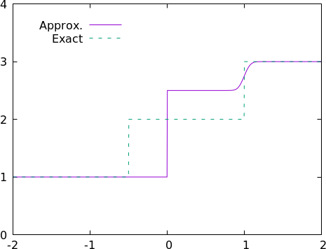
(a)

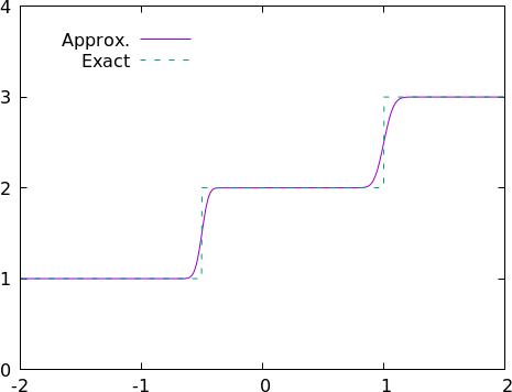
(b)

Figure 2: Approximation of a scalar conservation equation with piecewise linear flux: (a) viscosity solely based on $\lambda_{12}$ given in (4.2); (b) viscosity based on an entropy inequality, Eq. (4.3) with the choice $k_{i}=\frac{1}{2}({\mathsf{U}}_{i}^{\min,n}+{\mathsf{U}}_{i}^{\max,n}).$

This example is meant to demonstrate that only using the wave speed $\lambda_{12}$ defined in (4.2) to construct the graph viscosity (i.e., only using the Roe average) is not robust even in a case as simple as the one above. Using the wave speed $\lambda_{12}$ guarantees that the maximum principle locally holds, but the approximation may converge to a nonentropic weak solution. We illustrate this phenomenon by applying the algorithm described in the paper over the domain $D=(-2,2)$ using uniform meshes. The solution is computed to a final time $t=0.5$ using CFL=0.75. We show in the left panel of Figure 2 the solution obtained with the viscosity computed by using only $\lambda_{12}$. The graph of the exact solution is shown with a dashed line. We observe that the approximate solution does not converge to the exact solution. The leftmost discontinuity in the approximate solution is stationary instead of moving to the left at speed $-1$. The right panel shows the approximate solution using definition (4.3) for the wave speed with $k_{i}=\frac{1}{2}({\mathsf{U}}_{i}^{\min,n}+{\mathsf{U}}_{i}^{\min,n})$ for every $i\in{\mathcal{V}}$. We have verified that the method using this definition for the wave speed converges with the expected rate (tables not shown here for brevity).

6.2 1D non-convex flux

We now consider a Riemann problem in one space dimension using the scalar flux $f(v)=\sin(v)$. The initial data is $u_{0}(x)=(2+a)\pi$ if $x<0$ and $u_{0}(x)=b\pi$ otherwise. Here, $a\in[\frac{1}{2},1]$ and $b\in[0,\frac{1}{2}]$ are two chosen parameters. Note that the flux is neither convex nor concave over the interval $[b\pi,(2+a)\pi]$. Since $(2+a)\pi>b\pi$, the solution is obtained by replacing the flux by its upper concave envelope which is ${f\raisebox{6.0pt}{\tiny$\frown$}}(v)=\sin(v)$ for $v\in[b\pi,\frac{1}{2}\pi]$, ${f\raisebox{6.0pt}{\tiny$\frown$}}(v)=1$ for $v\in[\frac{1}{2}\pi,\frac{5}{2}\pi]$, and ${f\raisebox{6.0pt}{\tiny$\frown$}}(v)=\sin(v)$ for $v\in[\frac{5}{2}\pi,(2+a)\pi]$ (see, e.g., Dafermos [1, Lem. 3.1] and Holden and Risebro [13, §2.2]). We note that the entire the interval $v\in[\frac{1}{2}\pi,\frac{5}{2}\pi]$ is composed of sonic points. The exact solution is given by

(6.2) $$u(x,t)=\begin{cases}(2+a)\pi&\text{if $x\leq t\cos((2+a)\pi)$}\\ 3\pi-\arccos(|x/t|)&\text{if $t\cos((2+a)\pi)<x\leq 0$}\\ \arccos(x/t)&\text{if $0<x\leq t\cos(b\pi)$}\\ b\pi&\text{if $t\cos(b\pi)<x$}.\end{cases}$$

It is a composite wave composed of an expansion followed by a stationary shock followed by a second expansion. The numerical tests reported below are done with $b=0$ and $a=1$ over the domain $D=(-1,1)$.

Here again, tests done with the graph viscosity solely based on the Roe average $\lambda_{12}$ yields a method that is not robust (figures and tables are not reported for brevity). We observe that the approximate solution is a stationary shock for every mesh refinement (i.e., the initial data does not evolve), which is clearly not the entropy solution. One can artificially try to avoid this problem by initializing the approximate solution at $t_{0}>0$ using the exact solution (6.2). If the mesh does not have a vertex located at $\{0\}$, then convergence starts only when the mesh size is less that $t_{0}$. On the other hand, we observe convergence with no pre-asymptotic range for every positive value of $t_{0}$ when the mesh has a vertex located at $\{0\}$. This behavior illustrates well the lack of robustness of methods that are solely based on the wave speed $\lambda_{12}$.

We now test the method based on the wave speed computed by using (4.3). The tests are done with $\text{CFL}=0.5$. The relative errors in the $L^{1}$-norm and $L^{2}$-norm are computed at $t=0.8$. We test two strategies to select the Krǔzkov entropy for each degree of freedom $i\in{\mathcal{V}}$. The first strategy consists of setting $k_{i}=\theta{\mathsf{U}}_{i}^{\min,n}+(1-\theta){\mathsf{U}}_{i}^{\max,n}$ where $\theta=\frac{1}{2}$. The second strategy consists of setting $k_{i}=\theta_{i}{\mathsf{U}}_{i}^{\min,n}+(1-\theta_{i}){\mathsf{U}}_{i}^{\max,n}$, where $\theta_{i}\in(0,1)$ is a uniformly distributed random number changing at every grid point $i\in{\mathcal{V}}$.

	Random entropy				Average entropy
# dofs	$\delta^{1}(t)$	rate	$\delta^{2}(t)$	rate	$\delta^{1}(t)$	rate	$\delta^{2}(t)$	rate
51	1.96E-02	–	2.21E-02	–	2.41E-02	–	2.30E-02	–
101	1.39E-02	0.49	1.65E-02	0.42	1.81E-02	0.41	1.77E-02	0.38
201	9.17E-03	0.60	1.13E-02	0.55	1.33E-02	0.45	1.38E-02	0.35
401	5.87E-03	0.64	8.25E-03	0.45	9.81E-03	0.43	1.14E-02	0.28
801	3.66E-03	0.68	5.76E-03	0.52	7.54E-03	0.38	9.89E-03	0.20
1601	2.24E-03	0.71	4.15E-03	0.47	6.10E-03	0.31	9.06E-03	0.13
3201	1.38E-03	0.70	2.89E-03	0.52	5.20E-03	0.23	8.62E-03	0.07
6401	8.50E-04	0.70	2.06E-03	0.49	4.65E-03	0.16	8.39E-03	0.04

Table 1: 1D two-sonic point problem. The second and fourth columns show relative errors in the $L^{1}$-norm and the $L^{2}$-norms using a random Krǔzkov entropy with $k=\theta u_{L}+(1-\theta)u_{R}$, where $\theta\in(0,1)$ is a uniformly distributed random value. The sixth and eight columns report relative errors in the $L^{1}$-norm and the $L^{2}$-norms obtained for the average Krǔzkov entropy with $k=\frac{1}{2}(u_{L}+u_{R})$.

When using the first strategy with fixed $\theta=\frac{1}{2}$ we observe exactly the same problems as reported above when only using $\lambda_{12}$. Irrespective of the location of the grid points, the approximate solution is a stationary shock when one initializes the approximate solution with the exact solution at $t_{0}=0$. Initializing with the exact solution (6.2) at $t_{0}=10^{-8}$ still produces a stationary shock when the point $\{x=0\}$ is not a vertex of the mesh, but a non trivial solution is obtained when the point $\{x=0\}$ is a vertex of the mesh. We show in the right part of Table 1 convergence results using $t_{0}=10^{-8}$ and uniform meshes with odd numbers of grid points. We observe some kind of convergence on coarse meshes, but eventually the error stalls and stagnates as the mesh is further refined. We have observed this behavior for every constant value of $\theta$. This is highly counter intuitive because the viscosity based on (4.3) is strictly larger than $\lambda_{12}$, and we have observed in the above paragraph that the approximate solution using $\lambda_{12}$ converges to the entropy solution when the point $\{x=0\}$ is a mesh vertex. Here again, we observe a clear lack of robustness even when the wave speed is augmented so as to guarantee one “entropy fix” per grid point.

We now discuss what happens when the Krǔzkov entropy is randomly chosen. All the problem mentioned above disappear when $\theta_{i}\in(0,1)$ is randomly chosen at every grid point. The method convergences whether there is a grid point at $\{0\}$ or not and whatever the initial time. In particular there is no problem setting $t_{0}=0$. We show convergence tests in the left panel of Table 1 with $t_{0}=0$. To be able to compare with the results displayed in the right part of the table, we have use the same meshes. The method is now clearly convergent and converges with the expected rates.

The conclusion of this section is that the method based on the greedy wave speed computed by using (4.3) with random Krǔzkov entropies is robust.

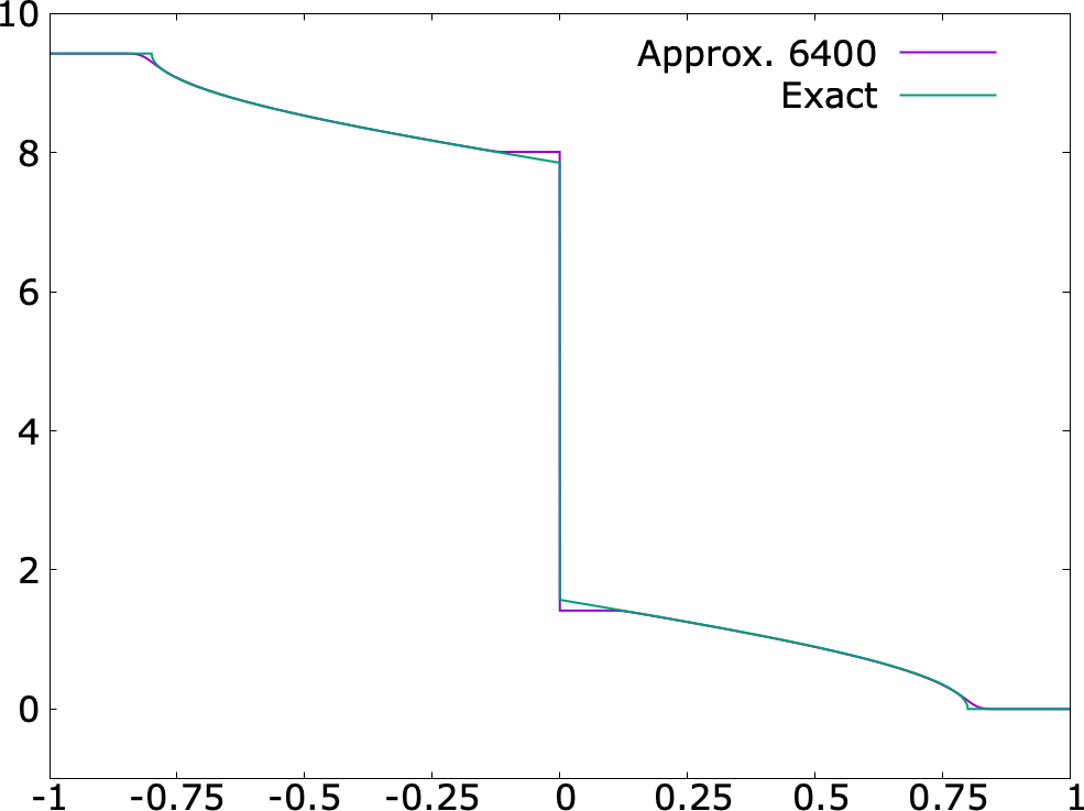
(a) Solution at $t=0.8$

	Square entropy $\eta(v)=\frac{1}{2}v^{2}$
# dofs	$\delta^{1}(t)$	rate	$\delta^{2}(t)$	rate
50	2.22E-02	–	2.18E-02	–
100	1.63E-02	0.45	1.64E-02	0.41
200	1.15E-02	0.50	1.23E-02	0.42
400	8.08E-03	0.51	9.44E-03	0.38
800	5.82E-03	0.47	7.61E-03	0.31
1600	4.38E-03	0.41	6.50E-03	0.23
3200	3.48E-03	0.33	5.87E-03	0.15
6400	2.92E-03	0.25	5.52E-03	0.09

(b) Convergence table

Figure 3: 1D two-sonic point problem computed with the square entropy $\eta(v)=\frac{1}{2}v^{2}$. The “entropy stable” method does not converge to the entropy solution.

Remark 6.1 (Robustness and “entropy stability”).

The numerical tests performed in this section demonstrates that robustness comes from randomness of the Krǔzkov entropy. Note in passing that this series of tests casts doubt on the robustness of methods that are called entropy stable in the literature. Since these methods enforce only one fixed global entropy inequality (at the semi-discrete level), one may wonder whether they produce approximations that converge to the right solution for the above one-dimensional problem. In order to provide some numerical evidence in this matter, we adjust our method as introduced in §4.2 for the entropy $\eta(v)=\frac{1}{2}v^{2}$ which is usually invoked in the literature dedicated to entropy stable methods. Redoing the computations in the proof of Lemma 4.3 with the square entropy gives $\lambda=(2ab+d+\sqrt{\Delta})/(2(c-a^{2}))$ with $a{:=}\frac{1}{2}(u_{L}+u_{R})$, $b{:=}\frac{1}{2}({\bm{f}}(u_{L})-{\bm{f}}(u_{R})){\cdot}{\bm{n}}$, $c{:=}\eta(u_{L})+\eta(u_{R})$, $d=({\bm{q}}(u_{R})-{\bm{q}}(u_{L})){\cdot}{\bm{n}}$, $\Delta{:=}(2ab+d)^{2}-4b^{2}(a^{2}-c)$. The method thus produced is locally and globally entropy stable with respect to $\eta(v)=\frac{1}{2}v^{2}$, i.e., (3.11) holds. Convergence tests with this method are reported in Figure 3. These tests show that the approximation does not converge to the entropy solution (6.2). The convergence behavior is strange as the approximation seems to converge over a large pre-asymptotic range, but eventually, when the mesh is very fine, the approximation converges to a weak solution that is not the entropy solution. In conclusion, the method is definitely entropy stable for the square entropy but it is not convergent for non-convex fluxes; hence, it is not robust. $\square$

6.3 The 2D KPP problem

(a) $\lambda_{12}$ with (4.2)

(b) $\lambda^{\text{grdy}}$ with (4.3), $\theta_{i}=\tfrac{1}{2}$

(c) $\lambda^{\text{grdy}}$ with (4.3), $\theta_{i}$ random

Figure 4: 2D KPP problem with ${\mathbb{P}}_{1}$ elements on nonuniform Delaunay mesh (118850 grid points) at $t=1$, $\text{CFL}=0.5$, computed with three different strategies: (a) $\lambda_{\max}=\lambda_{12}$ using (4.2); (b) wave speed $\lambda^{\text{grdy}}$ computed with (4.3) using $k_{i}=\theta{\mathsf{U}}_{i}^{\min,n}+(1-\theta){\mathsf{U}}_{i}^{\max,n}$ with $\theta=\frac{1}{2}$; (c) wave speed $\lambda^{\text{grdy}}$ computed with (4.3) using $k_{i}=\theta_{i}{\mathsf{U}}_{i}^{\min,n}+(1-\theta_{i}){\mathsf{U}}_{i}^{\max,n}$ where $\theta_{i}\in(0,1)$ is a uniformly random number changing for every $i\in{\mathcal{V}}$. Only the solution in the right panel is the correct entropy solution.

We finish our numerical examples by solving a two-dimensional scalar conservation equation with the non-convex flux ${\bm{f}}(u):=(\sin u,\cos u)^{\mathsf{T}}$

(6.3) $$\partial_{t}u+\nabla{\cdot}{\bm{f}}(u)=0,\quad u({\bm{x}},0)=u_{0}({\bm{x}})=\begin{cases}\tfrac{14\pi}{4}&\mbox{if }\sqrt{x^{2}+y^{2}}\leq 1\\ \tfrac{\pi}{4}&\mbox{otherwise},\end{cases}$$

in the computational domain $D=[-2,2]{\times}[-2.5,1.5]$. The problem was originally proposed in Kurganov et al. [14]. The solution has a two-dimensional composite wave structure which high-order numerical schemes have difficulties to capture correctly. We approximate the solution with continuous ${\mathbb{P}}_{1}$ finite elements on nonuniform Delaunay triangulations up to a final time of $t=1$. We show in Figure 4 three results computed on a mesh with 118850 grid points with CFL=0.5. The solution shown in the leftmost panel is obtained by only using the wave speed $\lambda_{12}$ for computing the greedy viscosity. The solution in the midle panel is obtained with the the wave speed (4.3) and the Krǔzkov entropy using $k_{i}=\theta{\mathsf{U}}_{i}^{\min,n}+(1-\theta){\mathsf{U}}_{i}^{\max,n}$ with $\theta=\frac{1}{2}$. The solution in the rightmost panel is obtained with the the wave speed (4.3) and the Krǔzkov entropy using $k_{i}=\theta_{i}{\mathsf{U}}_{i}^{\min,n}+(1-\theta_{i}){\mathsf{U}}_{i}^{\max,n}$ where $\theta_{i}$ is a random number changing for every $i\in{\mathcal{V}}$. One may be mislead thinking that the solution in the middle panel is correct, but the only approximation that converges correctly is the one using the random entropy.

So, here again, our conclusion for scalar conservation equations is that robustness can be achieved for methods based on the greedy wave speed (4.3) provided the Krǔzkov entropies are chosen randomly. Any other choice is not robust.

7 p-System

We test the method on the p-system using the equation of state $p(v)=\frac{1}{\gamma}v^{\gamma}$ with $\gamma=3$. We consider a Riemann problem with left state ${\bm{u}}_{L}=(v_{L},\sqrt{(1-v_{L})(p(v_{L})-p(1))}$ and right state ${\bm{u}}_{R}=(v_{R},-\sqrt{(1-v_{R})(p(v_{R})-p(1))}$. The solution is composed of two shock waves when $v_{L},v_{R}>1$, and in this case $v^{*}=1$, $u^{*}=0$. For this test we set $v_{L}=1.5$ and $v_{R}=1000$. The left shock is weak and fast moving; the shock speed is close to $-0.6849$. The right shock is strong and slow; the shock speed is close to $1.827{\times}10^{-2}$.

The simulations are done in the computational domain $D{:=}(0,1)$. The initial data is ${\bm{u}}_{0}(x)={\bm{u}}_{L}$ if $x<0.8$ and ${\bm{u}}_{0}(x)={\bm{u}}_{R}$ otherwise. The relative error in the $L^{1}$-norm is computed at $t=0.7$. The relative error is the sum of the relative error on $v$ plus the relative error on $u$. Convergences test are done on a sequence of uniform meshes starting from $51$ grid points to $1601$ grid points. The results are shown in Table 2. The results in the first column are obtained by using the upper wave speed estimate $\widehat{\lambda}_{\max}$ given in (5.9). Those shown in the second column are obtained by using $\lambda_{\max}$ as defined in (5.7) where $v^{*}$ is computed with a Newton method with $10^{-10}$ tolerance. Those shown in the right column are obtain with the greedy viscosity $\lambda^{\text{grdy}}$ defined in §5.3-5.4.

	$\widehat{\lambda}_{\max}$		$\lambda_{\max}$		$\lambda^{\text{grdy}}$
# dofs	$\delta^{1}(t)$	rate	$\delta^{1}(t)$	rate	$\delta^{1}(t)$	rate
51	3.33E-01	–	1.93E-01	–	1.31E-01	–
101	2.41E-01	0.47	1.57E-01	0.30	1.18E-01	0.15
201	1.41E-01	0.78	6.58E-02	1.25	4.93E-02	1.25
401	7.59E-02	0.89	4.42E-02	0.58	3.65E-02	0.43
801	3.64E-02	1.06	2.09E-02	1.08	1.77E-02	1.05
1601	1.70E-02	1.10	9.07E-03	1.20	7.76E-03	1.19

Table 2: Convergence tests for the $p$ system for various choices of wave speed estimate.

We show in Figure 5 the graph of the $u$ component at the final time $t=0.7$. In the left panel the approximation is done with 101 uniform grid points. We show a closer view of the plateau separating the two shocks in the right panel. The number of grid points used in each case is: 101 in the top right panel; 401 in middle right panel; and 1600 in the bottom right panel. This series of simulations demonstrate well the gain in accuracy that can potentially be gained by using the greedy viscosity technique described in this paper.

Figure 5: Approximation of the $u$ component in the $p$ system, $t=0.5$.

8 Conclusions

We have presented a general strategy to compute the artificial viscosity in first-order approximation methods for hyperbolic systems. The technique is based on the estimation of a minimum wave speed guaranteeing that the approximation satisfies predefined invariant-domain properties and predefined entropy inequalities. This approach eliminates non-essential fast waves from the construction of the artificial viscosity, while preserving pre-assigned invariant-domain properties and entropy inequalities. One should however keep in mind that being invariant-domain preserving is in general not enough to have a method that is robust. Likewise ensuring only one entropy inequality is not a guarantee of robustness.

References

- Dafermos [1972] C. M. Dafermos. Polygonal approximations of solutions of the initial value problem for a conservation law. J. Math. Anal. Appl., 38:33–41, 1972.
- Guermond and Popov [2016] J.-L. Guermond and B. Popov. Invariant domains and first-order continuous finite element approximation for hyperbolic systems. SIAM J. Numer. Anal., 54(4):2466–2489, 2016.
- Guermond and Popov [2017a] J.-L. Guermond and B. Popov. Invariant domains and second-order continuous finite element approximation for scalar conservation equations. SIAM J. Numer. Anal., 55(6):3120–3146, 2017a.
- Guermond and Popov [2017b] J.-L. Guermond and B. Popov. Invariant Domains and Second-Order Continuous Finite Element Approximation for Scalar Conservation Equations. SIAM J. Numer. Anal., 55(6):3120–3146, 2017b.
- Guermond et al. [2017] J.-L. Guermond, B. Popov, L. Saavedra, and Y. Yang. Invariant domains preserving arbitrary Lagrangian Eulerian approximation of hyperbolic systems with continuous finite elements. SIAM J. Sci. Comput., 39(2):A385–A414, 2017.
- Guermond et al. [2018] J.-L. Guermond, M. Nazarov, B. Popov, and I. Tomas. Second-order invariant domain preserving approximation of the Euler equations using convex limiting. SIAM J. Sci. Comput., 40(5):A3211–A3239, 2018.
- Guermond et al. [2019a] J.-L. Guermond, B. Popov, and I. Tomas. Invariant domain preserving discretization-independent schemes and convex limiting for hyperbolic systems. Comput. Methods Appl. Mech. Engrg., 347:143–175, 2019a.
- Guermond et al. [2019b] J.-L. Guermond, B. B. Popov, and I. Tomas. Invariant domain preserving schemes for hyperbolic systems of conservation laws. Multimat, August 2019, Trento, Italy, https://www.osti.gov/biblio/1641823-invariant-domain-preserving-schemes-hyperbolic-systems-conservation-laws, 2019b.
- Harten and Hyman [1983] A. Harten and J. M. Hyman. Self-adjusting grid methods for one-dimensional hyperbolic conservation laws. J. Comput. Phys., 50(2):235–269, 1983.
- Harten et al. [1983] A. Harten, P. D. Lax, and B. van Leer. On upstream differencing and Godunov-type schemes for hyperbolic conservation laws. SIAM Rev., 25(1):35–61, 1983.
- Hoff [1979] D. Hoff. A finite difference scheme for a system of two conservation laws with artificial viscosity. Math. Comp., 33(148):1171–1193, 1979.
- Hoff [1985] D. Hoff. Invariant regions for systems of conservation laws. Trans. Amer. Math. Soc., 289(2):591–610, 1985.
- Holden and Risebro [2015] H. Holden and N. H. Risebro. Front tracking for hyperbolic conservation laws, volume 152 of Applied Mathematical Sciences. Springer, Heidelberg, second edition, 2015.
- Kurganov et al. [2007] A. Kurganov, G. Petrova, and B. Popov. Adaptive semidiscrete central-upwind schemes for nonconvex hyperbolic conservation laws. SIAM Journal on Scientific Computing, 29(6):2381–2401, 2007.
- Lax [1954] P. D. Lax. Weak solutions of nonlinear hyperbolic equations and their numerical computation. Comm. Pure Appl. Math., 7:159–193, 1954.
- Lax [1957] P. D. Lax. Hyperbolic systems of conservation laws. II. Comm. Pure Appl. Math., 10:537–566, 1957.
- Le Métayer and Saurel [2016] O. Le Métayer and R. Saurel. The noble-abel stiffened-gas equation of state. Physics of Fluids, 28(4):046102, 2016.
- Nessyahu and Tadmor [1990] H. Nessyahu and E. Tadmor. Nonoscillatory central differencing for hyperbolic conservation laws. J. Comput. Phys., 87(2):408–463, 1990.
- Osher [1983] S. Osher. The Riemann problem for nonconvex scalar conservation laws and Hamilton-Jacobi equations. Proc. Amer. Math. Soc., 89(4):641–646, 1983.
- Perthame and Shu [1996] B. Perthame and C.-W. Shu. On positivity preserving finite volume schemes for Euler equations. Numer. Math., 73(1):119–130, 1996.
- Petrova and Popov [1999] G. Petrova and B. Popov. Linear transport equations with discontinuous coefficients. Comm. Partial Differential Equations, 24(9-10):1849–1873, 1999.
- Shu and Osher [1988] C.-W. Shu and S. Osher. Efficient implementation of essentially non-oscillatory shock-capturing schemes. J. Comput. Phys., 77(2):439 – 471, 1988.
- Tadmor [1984] E. Tadmor. Numerical viscosity and the entropy condition for conservative difference schemes. Math. Comp., 43(168):369–381, 1984.
- Toro [2009] E. F. Toro. Riemann solvers and numerical methods for fluid dynamics. Springer-Verlag, Berlin, third edition, 2009. A practical introduction.
- Young [2002] R. Young. The -system. I. The Riemann problem. In The legacy of the inverse scattering transform in applied mathematics (South Hadley, MA, 2001), volume 301 of Contemp. Math., pages 219–234. Amer. Math. Soc., Providence, RI, 2002.