On Representation Complexity of Model-based and Model-free Reinforcement Learning

Abstract

We study the representation complexity of model-based and model-free reinforcement learning (RL) in the context of circuit complexity. We prove theoretically that there exists a broad class of MDPs such that their underlying transition and reward functions can be represented by constant depth circuits with polynomial size, while the optimal $Q$-function suffers an exponential circuit complexity in constant-depth circuits. By drawing attention to the approximation errors and building connections to complexity theory, our theory provides unique insights into why model-based algorithms usually enjoy better sample complexity than model-free algorithms from a novel representation complexity perspective: in some cases, the ground-truth rule (model) of the environment is simple to represent, while other quantities, such as $Q$-function, appear complex. We empirically corroborate our theory by comparing the approximation error of the transition kernel, reward function, and optimal $Q$-function in various Mujoco environments, which demonstrates that the approximation errors of the transition kernel and reward function are consistently lower than those of the optimal $Q$-function. To the best of our knowledge, this work is the first to study the circuit complexity of RL, which also provides a rigorous framework for future research.

1 Introductions

In recent years, reinforcement learning (RL) has seen significant advancements in various real-world applications (Mnih et al., 2013; Silver et al., 2016; Moravčík et al., 2017; Shalev-Shwartz et al., 2016; Yurtsever et al., 2020; Yu et al., 2020; Kober et al., 2014). Roughly speaking, the RL algorithms can be categorized into two types: model-based algorithms (Draeger et al., 1995; Rawlings, 2000; Luo et al., 2018; Chua et al., 2018; Nagabandi et al., 2020; Moerland et al., 2023) and model-free algorithms (Mnih et al., 2015; Lillicrap et al., 2015; Van Hasselt et al., 2016; Haarnoja et al., 2018). Model-based algorithms typically learn the underlying dynamics of the model (i.e., the transition kernel and the reward function) and then learn the optimal policy utilizing the knowledge of the ground-truth model. On the other hand, model-free algorithms usually derive optimal policies through different quantities, such as $Q$-function and value function, without directly assimilating the underlying ground-truth models.

In statistical machine learning, the efficiency of an algorithm is usually measured by sample complexity. For the comparison of model-based and model-free RL algorithms, many previous works also focus on their sample efficiency gap, and model-based algorithm usually enjoys a better sample complexity than model-free algorihms (Jin et al., 2018; Zanette and Brunskill, 2019; Tu and Recht, 2019; Sun et al., 2019). In general, the error of learning  can be decomposed into three parts: optimization error, statistical error, and approximation error. Many previous efforts focus on optimization errors (Singh et al., 2000; Agarwal et al., 2020; Zhan et al., 2023) and statistical errors Kakade (2003); Strehl et al. (2006); Auer et al. (2008); Azar et al. (2017); Rashidinejad et al. (2022); Zhu and Zhang (2023), while approximation error has been less explored. Although a line of previous work studies the sample complexity additionally caused by the approximation error under the assumption of a bounded model misspecification error (Jin et al., 2019; Wang et al., 2020; Zhu et al., 2023b; Huang et al., 2021; Zhu et al., 2023a), they did not take a further or deeper step to study for what types of function classes (including transition kernel, reward function, $Q$-function, etc.), it is reasonable to assume a small model misspecification error.

In this paper, we study approximation errors through the lens of representation complexities. Intuitively, if a function (transition kernel, reward function, $Q$-function, etc.) has a low representation complexity, it would be relatively easy to learn it within a function class of low complexity and misspecification error, thus implying a better sample complexity. The previous work Dong et al. (2020b) studies a special class of MDPs with state space $\mathcal{S}=[0,1]$, action space $\mathcal{A}=\{0,1\}$, transition kernel piecewise linear with constant pieces and a simple reward function. By showing that the optimal $Q$-function requires an exponential number of linear pieces to approximate, they provide a concrete example that the $Q$-function has a much larger representation complexity than the transition kernel and reward function, which implies that model-based algorithms enjoy better sample complexity. However, the MDP class they study is restrictive. Thus, it is unclear whether it is a universal phenomenon that the underlying models have a lower representation complexity than other quantities such as $Q$-functions. Moreover, their metrics of measuring representation complexity, i.e., the number of pieces of piece-wise linear functions, is not fundamental, rigorous, or applicable to more general functions.

Therefore, we study representation complexity via circuit complexity (Shannon, 1949), which is a fundamental and rigorous metric that can be applied to arbitrary functions stored in computers. Also, since the circuit complexity has been extensively explored by numerous previous works (Shannon, 1949; Karp, 1982; Furst et al., 1984; Razborov, 1989; Smolensky, 1987; Vollmer, 1999; Leighton, 2014) and is still actively evolving, it could offer us a deep understanding of the representation complexity of RL, and any advancement of circuit complexity might provide new insights into our work. Theoretically, we show that there exists a general class of MDPs called Majority MDP (see more details in Section 3), such that their transition kernels and reward functions have much lower circuit complexity than their optimal $Q$-functions. This provides a new perspective for the better sample efficiency of model-based algorithms in more general settings. We also empirically validate our results by comparing the approximation errors of the transition kernel, reward function, and optimal $Q$-function in various Mujoco environments (see Section 4 for more details).

We briefly summarize our main contributions as follows:

• We are the first to study the representation complexity of RL under a circuit complexity framework, which is more fundamental and rigorous than previous works.

• We study a more general class of MDPs than previous work, demonstrating that it is common in a broad scope that the underlying models are easier to represent than other quantities such as $Q$-functions.

• We empirically validate our results in real-world environments by comparing the approximation error of the ground-truth models and $Q$-functions in various MuJoCo environments.

1.1 Related work

Model-based v.s. Model-free algorithms.

Many previous results imply that there exists the sample efficiency gap between model-based and model-free algorithms in various settings, including tabular MDPs (Strehl et al., 2006; Azar et al., 2017; Jin et al., 2018; Zanette and Brunskill, 2019), linear quadratic regulators (Dean et al., 2018; Tu and Recht, 2018; Dean et al., 2020), contextual decision processes with function approximation (Sun et al., 2019), etc. The previous work Dong et al. (2020b) compares model-based and model-free algorithms through the lens of the expressivity of neural networks. They claim that the expressivity is a different angle from sample efficiency. On the contrary, in our work, we posit the representation complexity as one of the important reasons causing the gap in sample complexity.

Ground-truth dynamics.

The main result of our paper is that, in some cases, the underlying ground-truth dynamics (including the transition kernels and reward models) are easier to represent and thus learn, which inspires us to utilize the knowledge of the ground-truth model to boost the learning algorithms. This is consistent with the methods of many previous algorithms that exploit the dynamics to boost model-free quantities (Buckman et al., 2018; Feinberg et al., 2018; Luo et al., 2018; Janner et al., 2019), perform model-based planning (Oh et al., 2017; Weber et al., 2017; Chua et al., 2018; Wang and Ba, 2019; Piché et al., 2018; Nagabandi et al., 2018; Du and Narasimhan, 2019) or improve the learning procedure via various other approaches (Levine and Koltun, 2013; Heess et al., 2015; Rajeswaran et al., 2016; Silver et al., 2017; Clavera et al., 2018).

Approximation error.

A line of previous work (Jin et al., 2019; Wang et al., 2020; Zhu et al., 2023b) study the sample complexity of RL algorithms in the presence of model misspecification. This bridges the connection between the approximation error and sample efficiency. However, these works directly assume a small model misspecification error without further justifying whether it is reasonable. Our results imply that assuming a small error of transition kernel or reward function might be more reasonable than $Q$-functions. Many other works study the approximation error and expressivity of neural networks (Bao et al., 2014; Lu et al., 2017; Dong et al., 2020a; Lu et al., 2021). Instead, we study approximation error through circuit complexity, which provides a novel perspective and rigorous framework for future research.

Circuit complexity.

Circuit complexity is one of the most fundamental concepts in the theory of computer science (TCS) and has been long and extensively explored (Savage, 1972; Valiant, 1975; Trakhtenbrot, 1984; Furst et al., 1984; Hastad, 1986; Smolensky, 1987; Razborov, 1987, 1989; Boppana and Sipser, 1990; Arora and Barak, 2009). In this work, we first introduce circuit complexity to reinforcement learning to study the representation complexity of different functions including transition kernel, reward function and $Q$-functions, which bridges an important connection between TCS and RL.

1.2 Notations

Let $\mathbf{1}_{b}=(1,\dots,1)\in\mathbb{R}^{b}$ denote the all-one vector and let $\mathbf{0}_{b}=(0,\dots,0)\in\mathbb{R}^{b}$ denote the all-zero vector. For any set $\mathcal{X}$ and any function $f:\mathcal{X}\to\mathcal{X}$, $f^{(k)}(x)$ is the value of $f$ applied to $x$ after $k$ times, i.e., $f^{(1)}(x)=f(x)$ and $f^{(k)}(x)=\underbrace{f(f(\dots f}_{k}(x))\dots))$.

Let $\lceil x\rceil$ denote the smallest integer greater than or equal to $x$, and let $\lfloor x\rfloor$ denote the greatest integer less than or equal to $x$. We use $\{0,1\}^{n}$ to denote the set of $n$-bits binary strings. Let $\delta_{x}$ denote the Dirac measure: $\delta_{x}(A)=\begin{cases}1,&~{}x\in A\\ 0,&~{}x\notin A\end{cases}$ and we use $\mathbbm{1}(\cdot)$ to denote the indicator function. Let $[n]$ denote the set $\{1,2,\dots,n\}$ and let $\mathbb{N}=\{0,1,2,\ldots\}$ denote the set of all natural numbers.

2 Preliminaries

2.1 Markov Decision Process

An episodic Markov Decision Process (MDP) is defined by the tuple $\mathcal{M}=(\mathcal{S},\mathcal{A},H,\mathbb{T},r)$ where $\mathcal{S}$ is the state space, $\mathcal{A}$ is the action set, $H$ is the number of time steps in each episode, $\mathbb{T}$ is the transition kernel from $\mathcal{S}\times\mathcal{A}$ to $\Delta(\mathcal{S})$ and $r=\{r_{h}\}_{h=1}^{H}$ is the reward function. When $\mathbb{T}(\cdot|s,a)=\delta_{s^{\prime}}$, i.e., $\mathbb{T}$ is deterministic, we also write $\mathbb{T}(s,a)=s^{\prime}$. In each episode, the agent starts at a fixed initial state $s_{1}$ and at each time step $h\in[H]$ it takes action $a_{h}$, receives reward $r_{h}(s_{h},a_{h})$ and transits to $s_{h+1}\sim\mathbb{T}(\cdot|s_{h},a_{h})$. Typically, we assume $r_{h}(s_{h},a_{h})\in[0,1]$.

A policy $\pi$ is a length-$H$ sequence of functions $\pi=\{\pi_{h}:\mathcal{S}\mapsto\Delta(\mathcal{A})\}_{h=1}^{H}$. Given a policy $\pi$, we define the value function $V_{h}^{\pi}(s)$ as the expected cumulative reward under policy $\pi$ starting from $s_{h}=s$ (we abbreviate $V^{*}:=V^{*}_{0}$):

$$V_{h}^{\pi}(s):=\mathbb{E}\left.\left[\sum_{t=h}^{H}r_{t}(s_{t},a_{t})\right|s_{h}=s,\pi\right]$$

and we define the $Q$-function $Q_{h}^{\pi}(s,a)$ as the the expected cumulative reward taking action $a$ in state $s_{h}=s$ and then following $\pi$ (we abbreviate $Q^{*}:=Q^{*}_{0}$):

$$Q_{h}^{\pi}(s,a):=\mathbb{E}\left.\left[\sum_{t=h}^{H}r_{t}(s_{t},a_{t})\right|s_{h}=s,a_{h}=a,\pi\right].$$

The Bellman operator $\mathcal{T}_{h}$ applied to $Q$-function $Q_{h+1}$ is defined as follow

$$\mathcal{T}_{h}(Q_{h+1})(s,a):=r_{h}(s,a)+\mathbb{E}_{s^{\prime}\sim\mathbb{T}(\cdot|s,a)}[\max_{a^{\prime}}Q_{h+1}(s^{\prime},a^{\prime})].$$

There exists an optimal policy $\pi^{\ast}$ that gives the optimal value function for all states, i.e. $V^{\pi^{\ast}}_{h}(s)=\sup_{\pi}V_{h}^{\pi}(s)$ for all $h\in[H]$ and $s\in\mathcal{S}$ (see, e.g., Agarwal et al. (2019)). For notation simplicity, we abbreviate $V^{\pi^{\ast}}$ as $V^{\ast}$ and correspondingly $Q^{\pi^{\ast}}$ as $Q^{\ast}$. Therefore $Q^{\ast}$ satisfies the following Bellman optimality equations for all $s\in\mathcal{S}$, $a\in\mathcal{A}$ and $h\in[H]$:

$$Q^{\ast}_{h}(s,a)=\mathcal{T}_{h}(Q^{\ast}_{h+1})(s,a).$$

2.2 Function approximation

In value-based (model-free) function approximation, the learner is given a function class $\mathcal{F}=\mathcal{F}_{1}\times\cdots\times\mathcal{F}_{H}$, where $\mathcal{F}_{h}\subset\{f:\mathcal{S}\times\mathcal{A}\mapsto[0,H]\}$ is a set of candidate functions to approximate the optimal Q-function $Q^{\ast}$.

In model-based function approximation, the learner is given a function class $\mathcal{F}=\mathcal{F}_{1}\times\cdots\times\mathcal{F}_{H}$, where $\mathcal{F}_{h}\subset\{f:\mathcal{S}\times\mathcal{A}\mapsto\Delta(\mathcal{S})\}$ is a set of candidate functions to approximate the underlying transition function $\mathbb{T}$. Additionally, the learner might also be given a function class $\mathcal{R}=\mathcal{R}_{1}\times\cdots\times\mathcal{R}_{H}$ where $\mathbb{R}_{h}\subset\{f:\mathcal{S}\times\mathcal{A}\mapsto[0,1]\}$ is a set of candidate functions to approximate the reward function $r$. Typically, the reward function would be much easier to learn than the transition function.

To learn a function with a large representation complexity, one usually needs a function class with a large complexity to ensure that the ground-truth function is (approximately) realized in the given class. A larger complexity (e.g., log size, log covering number, etc.) of the function class would incur a larger sample complexity. Our main result shows that it is common that an MDP has a transition kernel and reward function with low representation complexity while the optimal $Q$-function has a much larger representation complexity. This implies that model-based algorithms might enjoy better sample complexity than value-based (model-free) algorithms.

2.3 Circuit complexity

To provide a rigorous and fundamental framework for representation complexity, in this paper, we use circuit complexity to measure the representation complexity.

Circuit complexity has been extensively explored in depth. In this section, we introduce concepts related to our results. One can refer to Arora and Barak (2009); Vollmer (1999) for more details.

Definition 1 (Boolean circuits, adapted from Definition 6.1, Arora and Barak (2009)).

For every $m,n\in\mathbb{Z}_{+}$, a Boolean circuit $C$ with $n$ inputs and $m$ outputs is a directed acyclic graph with $n$ sources and $m$ sinks (both ordered). All non-source vertices are called gates and are labeled with one of $\wedge$ (AND), $\vee$ (OR) or $\neg$ (NOT). For each gate, its fan-in is the number of incoming edges, and its fan-out is the number of outcoming edges. The size of $C$ is the number of vertices in it. The depth of $C$ is the length of the longest directed path in it. A circuit family is a sequence $\{C_{n}\}_{n\in\mathbb{Z}_{+}}$ of Boolean circuits where $C_{n}$ has $n$ inputs.

If $C$ is a Boolean circuit, and $x=(x_{1},\dots,x_{n})\in\{0,1\}^{n}$ is its input, then the output of $C$ on $x$, denoted by $C(x)$, is defined in the following way: for every vertex $v$ of $C$, a value $\mathrm{val}(v)$ is assigned to $v$ such that $\mathrm{val}(v)$ is given recursively by applying $v$’s logical operation on the values of the vertices pointed to $v$; the output $C(x)$ is a $m$-bits binary string $y=(y_{1},\dots,y_{m})$, where $y_{i}$ is the value of the $i$-th sink.

Definition 2 (Circuit computation).

A circuit family is a sequence $C=(C_{1},C_{2},\ldots,C_{n},\ldots)$, where for every $n\in\mathbb{Z}_{+}$, $C_{n}$ is a Boolean circuit with $n$ inputs. Let $f_{n}$ be the function computed by $C_{n}$ . Then we say that $C$ computes the function $f:\{0,1\}^{*}\to\{0,1\}^{*}$, which is defined by

$$f(w):=C_{|w|}(w),~{}\forall w\in\{0,1\}^{*}$$

where $|w|$ is the bit length of $w$. More generally, we say that a function $f:\mathbb{N}\to\mathbb{N}$ can be computed by $C$ if $f$ can be computed by $C$ where the inputs and the outputs are represented by binary numbers.

Definition 3 ($(k,m)$-DNF).

A $(k,m)$-DNF is a disjunction of conjuncts, i.e., a formula of the form

$$\bigvee_{i=1}^{n}\left(\bigwedge_{j=1}^{k_{i}}X_{i,j}\right)$$

where $k_{i}\leq k$ for every $i\in[n]$, $\sum_{i=1}^{n}k_{i}\leq m$, and $X_{i,j}$ is either a primitive Boolean variable or the negation of a primitive Boolean variable.

Definition 4 ($\mathbf{AC}^{0}$).

$\mathbf{AC}^{0}$ is the class of all boolean functions $f:\{0,1\}^{*}\to\{0,1\}^{*}$ for which there is a circuit family with unbounded fan-in, $n^{O(1)}$ size, and constant depth that computes $f$.

In this paper, we study representation complexity within the class of constant-depth circuits. Our results depend on two “hard” functions, parity and majority functions, which require exponential size circuits to compute and thus are not in $\mathbf{AC}^{0}$. Below, we formally define these two functions respectively.

Definition 5 (Parity).

For every $n\in\mathbb{Z}_{+}$, the $n$-variable parity function $\mathsf{PARITY}_{n}:\{0,1\}^{n}\to\{0,1\}$ is defined by $\mathsf{PARITY}_{n}(x_{1},\dots,x_{n})=\sum_{i=1}^{n}x_{i}~{}\mod 2$. The parity function $\mathsf{PARITY}:\{0,1\}^{*}\to\{0,1\}$ is defined by

$$\mathsf{PARITY}(w):=\mathsf{PARITY}_{|w|}(w),~{}\forall w\in\{0,1\}^{*}.$$

Proposition 2.1 (Furst et al. (1984)).

$\mathsf{PARITY}\notin\mathbf{AC}^{0}$.

3 Theoretical Results

We show our main results in this section that there exists a broad class of MDPs that demonstrates a separation between the representation complexity of the ground-truth model and that of the value function. This reveals one of the important reasons that model-based algorithms usually enjoy better sample efficiency than value-based (model-free) algorithms.

The previous work Dong et al. (2020b) also conveyed similar messages. However, they only study a very special MDP while we study a more general class of MDPs. Moreover, Dong et al. (2020b) measures the representation complexity of functions by the number of pieces for a piecewise linear function, which is not rigorous and not applicable to more general functions.

To study the representation complexity of MDPs under a more rigorous and fundamental framework, we introduce circuit complexity to facilitate the study of representation complexity. In this work, we focus on circuits with constant-depth. We first show a warm-up example in Section 3.1, and then extend our results to a broader class of MDPs in Section 3.2.

3.1 Warm up example

In this section we show a simple MDP that demonstrates a separation between the circuit complexity of the model function and that of the value function.

Definition 6 (Parity MDP).

An $n$-bits parity MDP is defined as follows: the state space is $\{0,1\}^{n}$, the action space is $\{(i,j):i,j\in[n]\}$, and the planning horizon is $H=n$. Let the reward function be defined by: $r(s,a)=\begin{cases}1,&~{}s=\mathbf{0}_{n}\\ 0,&~{}\text{otherwise}\end{cases}$. Let the transition function be defined as follows: for each state $s$ and action $a=(i,j)$, transit with probability $1$ to $s^{\prime}$ where $s^{\prime}$ is given by flipping the $i$-th and $j$-th bits of $s$.

Both $\mathbb{T}$ and $r$ can be computed by a circuit with polynomial-size and constant depth. Indeed, consider the following circuit:

$$C_{\mathrm{reward}}(s)=s_{1}\wedge s_{2}\wedge\cdots\wedge s_{n}.$$

It can be verified that $C_{\mathrm{reward}}=r$ and it has size $n$. For the model transition function, we consider the binary representation of the action: for each $a=(i,j)$, let $(a_{1},\dots,a_{b})$ denote the binary representation of $i$ and let $(a_{b+1},\dots,a_{2b})$ denote the binary representation of $j$, where $b=\lceil\log(n+1)\rceil$. Then define the following circuit:

$$C_{\mathrm{model}}(s,a)=\left(s_{k}\oplus\delta_{k}(a_{1},\dots,a_{b})\oplus\delta_{k}(a_{b+1},\dots,a_{2b})\right)_{k=1}^{n}$$

where $\oplus$ is the XOR gate and $\delta_{k}(x_{1},\dots,x_{b})=\mathbbm{1}\left(k=\sum_{i=1}^{b}2^{b-i}\cdot x_{i}\right)$. We visualize this circuit in Figure 1.

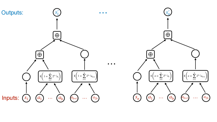
Figure 1: Constant-depth circuit of the model transition function in parity MDP. An empty node is directly assigned the value of the node pointing to it.

Since the XOR gate and the gate $\delta_{k}$ can all be implemented by binary circuits with polynomial size and constant depth (notice that $a\oplus b=(\neg a\vee b)\wedge(a\vee\neg b)$ and $\delta_{k}(x_{1},\dots,x_{b})=(x_{1}\vee k_{1})\vee\cdots\vee(x_{b}\vee k_{b})$ where $k_{1}k_{2}\cdots k_{b}$ is the binary representation of $k$), $C_{\mathrm{model}}$ also has polynomial size and constant depth.

However, the optimal $Q$-function $Q^{*}$ can not be computed by a circuit with polynomial size and constant depth. Indeed, it suffices to see that the value function $V^{*}$ can not be computed by a circuit with polynomial size and constant depth. To see this, notice that $\mathbbm{1}(V^{*}>0)$ is the parity function, since if there are even numbers of 1’s in $(s_{1},\dots,s_{n})$, then there always exists a sequence of actions to transit to the reward state; otherwise, the number of 1’s remains odd and will never become $\mathbf{0}_{n}$. Suppose for the sake of contradiction that there exists a circuit $C_{\mathrm{value}}$ with polynomial size and constant depth that computes $V^{*}$, then the circuit

$$C_{\mathsf{PARITY}}(s,a)=C_{\mathrm{value}}(s,a)_{1}\vee C_{\mathrm{value}}(s,a)_{2}\vee\cdots\vee C_{\mathrm{value}}(s,a)_{n}$$

computes the parity function for $s$ and belongs to the class $\mathbf{AC}^{0}$. This contradicts Proposition 2.1.

3.2 A broader family of MDPs

In this section, we present our main results, i.e., there exists a general class of MDP, of which nearly all instances of MDP have low representation complexity for the transition model and reward function but suffer an exponential representation complexity for the optimal $Q$-function.

We consider a general class of MDPs called ‘majority MDP’, where the states are comprised of representation bits that reflect the situation in the underlying environment and control bits that determine the transition of the representation bits. We first give the definition of majority MDP and then provide intuitive explanations.

Definition 7 (Control function).

We say that a map $f$ from $\{0,1\}^{b}$ to itself is a control function over $\{0,1\}^{b}$, if $f(\mathbf{1}_{b})=\mathbf{1}_{b}$, and

$$\left\{f^{(k)}(\mathbf{0}_{b}):k=1,2,\dots,2^{b}-1\right\}=\{0,1\}^{b}\backslash\{\mathbf{0}_{b}\}.$$

Definition 8 (Majority MDP).

An $n$-bits majority MDP with reward state $s_{\mathrm{reward}}\in\{0,1\}^{n}$, control function $f:\{0,1\}^{\lceil\log(n+1)\rceil}\to\{0,1\}^{\lceil\log(n+1)\rceil}$, and condition $C:\{0,1\}^{n}\to\{0,1\}$ is defined by the following:

• The state space is given by $\{0,1\}^{n+b}$ where $b=\lceil\log(n+1)\rceil$. For convenience, we assume $n=2^{b}-1$. Each state is comprised of two subparts $s=(s[c],s[r])$, where $s[c]=(s_{1},\dots,s_{b})\in\{0,1\}^{b}$ is called the control bits, and $s[r]=(s_{b+1},\dots,s_{b+n})\in\{0,1\}^{n}$ is called the representation bits (see Figure 2);

• The action space is $\{0,1\}$; The planning horizon is $H=2^{b}+n$;

• The reward function is defined by: $r(s,a)=\begin{cases}1,&~{}s[r]=s_{\mathrm{reward}},s[c]=\mathbf{1}_{b}\\ 0,&~{}\text{otherwise}\end{cases}$;

• The transition function $\mathbb{T}$ is defined as follows: define the flipping function $g:\{0,1\}^{n}\times[n]\to\{0,1\}^{n}$ by $g(s,i)=(s_{1},\dots,\neg s_{i},\dots,s_{n})$, then $\mathbb{T}$ is given by:

  $$\mathbb{T}(s,a)=\begin{cases}\left(s[c],g(s[r],\sum_{j=1}^{b}2^{b-j}\cdot s_{j})\right),&~{}a=1,C(s[r])=1\\ \left(f(s[c]),s[r]\right),&~{}\text{otherwise}\end{cases}$$

  that is, if $a=1$ and $C(s[r])=1$, then transit to $s^{\prime}=\left(s[c],g(s[r],i)\right)$ where $i=\sum_{j=1}^{b}2^{b-j}\cdot s_{j}$ and $g_{i}(s[r])$ is given by flipping the $i$-th bits of $s[r]$ (keep the control bits while flip the $i$-th coordinate of the representation bits); otherwise transit to $s^{\prime}=\left(f(s[c]),s[r]\right)$ (keep the representation bits and apply the control function $f$ to the control bits).

When $C\equiv 1$, we call such an MDP unconditioned.

Figure 2: Illustration of state for majority MDPs.

Although many other MDPs lie outside of the Majority MDP class, most are too random to become meaningful (for example, the MDP where the reward state is in a $o(n)$-sized connected component). Thus, instead of studying a more general class of MDPs, we consider one representative class of MDPs and separate three fundamental notions in RL: control, representation, and condition. We elaborate on these aspects in the following remark.

Remark 1 (Control function and control bits).

In Majority MDPs, the control bits start at $\mathbf{0}_{b}$ and traverse all $b$-bits binary strings before ending at $\mathbf{1}_{b}$. This means that the agent can can flip every entry of the representation bits, and therefore, the agent is able to change the representation bits to any $n$-bits binary string within $2^{b}+n$ time steps in unconditional settings.

The control function is able to express any ordering of $b$-bits strings (starting from $\mathbf{0}_{b}$ and ending with $\mathbf{1}_{b}$) in which the control bits are taken. With this expressive power, the framework of Majority MDP simplifies the action space to fundamental case of $\mathcal{A}=\{0,1\}$.

Remark 2 (Representation bits).

In general, the states of any MDP (even for MDP with continuous state space) are stored in computer systems in finitely many bits. Therefore, we allocate $n$ bits in the representation bits to encapsulate and delineate the various states within an MDP.

Remark 3 (Condition function).

The condition function simulates and expresses the rules of transition in an MDP. In many real-world applications, the decisions made by an agent only take effect (and therefore cause state transition) under certain underlying conditions, or only enable transitions to certain states that satisfy the conditions: for example, an marketing maneuver made by a company will only make an influence if it observes the advertisement law and regulations; a move of a piece chess must follow the chess rules; a treatment decision can only affect some of the measurements taken on an individual; a resource allocation is subject to budget constraints; etc.

Finally, the following two theorems show the separation result of circuit complexity between the model and the optimal $Q$-function for Majority MDP in both unconditional and conditional settings.

Theorem 1 (Separation result of majority MDP, unconditioned setting).

For any reward state $s_{\mathrm{reward}}\in\{0,1\}^{n}$ and any control function $f:\{0,1\}^{b}\to\{0,1\}^{b}$, the unconditioned $n$-bits majority MDP with reward state $s_{\mathrm{reward}}$, control function $f$ has the following properties:

• The reward function and the transition function can be computed by circuits with polynomial (in $n$) size and constant depth.

• The optimal Q-function (at time step $t=0$) cannot be computed by a circuit with polynomial size and constant depth.

Theorem 2 (Separation result of majority MDP, conditioned setting).

Fix $m<n/2$. Let $\rho$ be uniform distribution over $(O(1),m)$-DNFs of $n$ Boolean variables. Then for any reward state $s_{\mathrm{reward}}\in\{0,1\}^{n}$ and any control function $f:\{0,1\}^{b}\to\{0,1\}^{b}$, with probability at least $1-e^{-\Omega(m)}$, the $n$-bits majority MDP with reward state $s_{\mathrm{reward}}$, control function $f$, and condition $C$ sampled from $\rho$, has the following properties:

• The reward function and the transition function can be computed by circuits with polynomial (in $n$) size and constant depth.

• The optimal Q-function (at time step $t=0$) cannot be computed by a circuit with polynomial size and constant depth.

The proof of Theorem 1 and Theorem 2 are deferred to Section B.3 and Section B.2. In short, they imply that $\mathbb{T},r\in\mathbf{AC}_{0}$ and $Q^{*}\notin\mathbf{AC}_{0}$. In fact, we show that the value functions cannot be computed by a circuit with polynomial size and constant depth. Due to the relationship $Q^{*}(s,a)=r(s,a)+V^{*}(\mathbb{T}(s,a))$, we will treat these two functions synonymously and refer to them collectively as the "value function."

4 Experiments

Theorems 1 and 2 indicate that there exists a broad class of MDPs in which the transition functions and the reward functions have much lower circuit complexity than the optimal $Q$-functions (actually also value functions according to our proof for Majority MDPs). This observation, therefore, implies that value functions might be harder to approximate than transition functions and the reward functions, and gives rise to the following question:

In general MDPs, are the value functions harder to approximate than transition functions and the reward functions?

In this section, we seek to answer this question via experiments on common simulated environments. Specifically, we fix $d,m\in\mathbb{Z}_{+}$, and let $\mathcal{F}$ denote the class of $d$-depth, $m$-width neural networks (with input and output dimensions tailored to the context). The quantities of interest are the following relative approximation errors

$$e_{\text{model}}= ~{}\min_{P\in\mathcal{F}}\frac{\mathbb{E}[\|P(s,a)-\mathbb{T}(s,a)\|^{2}]}{\mathbb{E}[\|\mathbb{T}(s,a)\|^{2}]}$$

$$e_{\text{reward}}= ~{}\min_{R\in\mathcal{F}}\frac{\mathbb{E}[(R(s,a)-r(s,a))^{2}]}{\mathbb{E}[(r(s,a))^{2}]}$$

$$e_{\text{$Q$-function}}= ~{}\min_{Q\in\mathcal{F}}\frac{\mathbb{E}[(Q(s,a)-Q^{*}(s,a))^{2}]}{\mathbb{E}[(Q^{*}(s,a))^{2}]}$$

where the expectation is over the distribution of the optimal policy and the mean squared errors are divided by the second moment so that the scales of different errors will match. Therefore, $e_{\text{model}},e_{\text{reward}},e_{\text{Q-function}}$ stand for the difficulty for a $d$-depth, $m$-width neural networks to approximate the transition function, the reward function, and the $Q$-function, respectively.

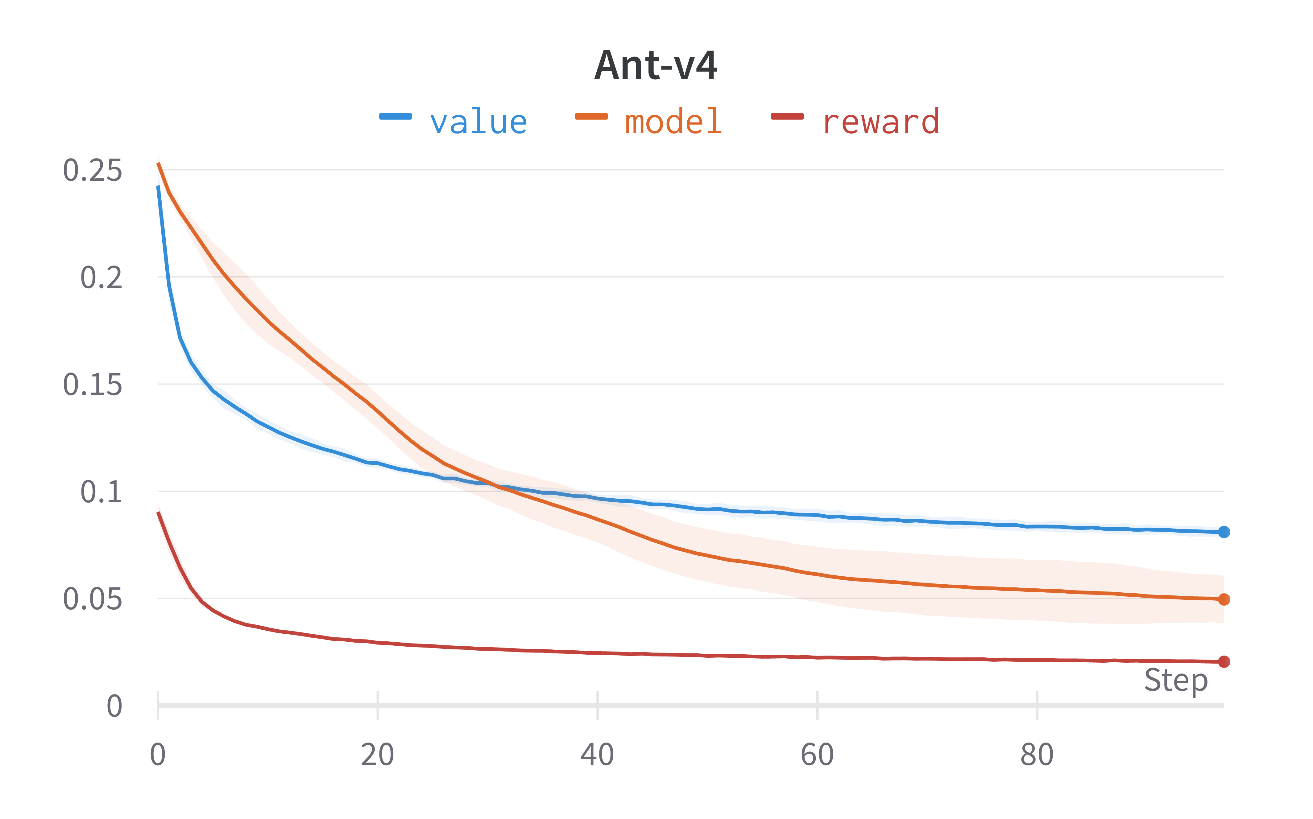
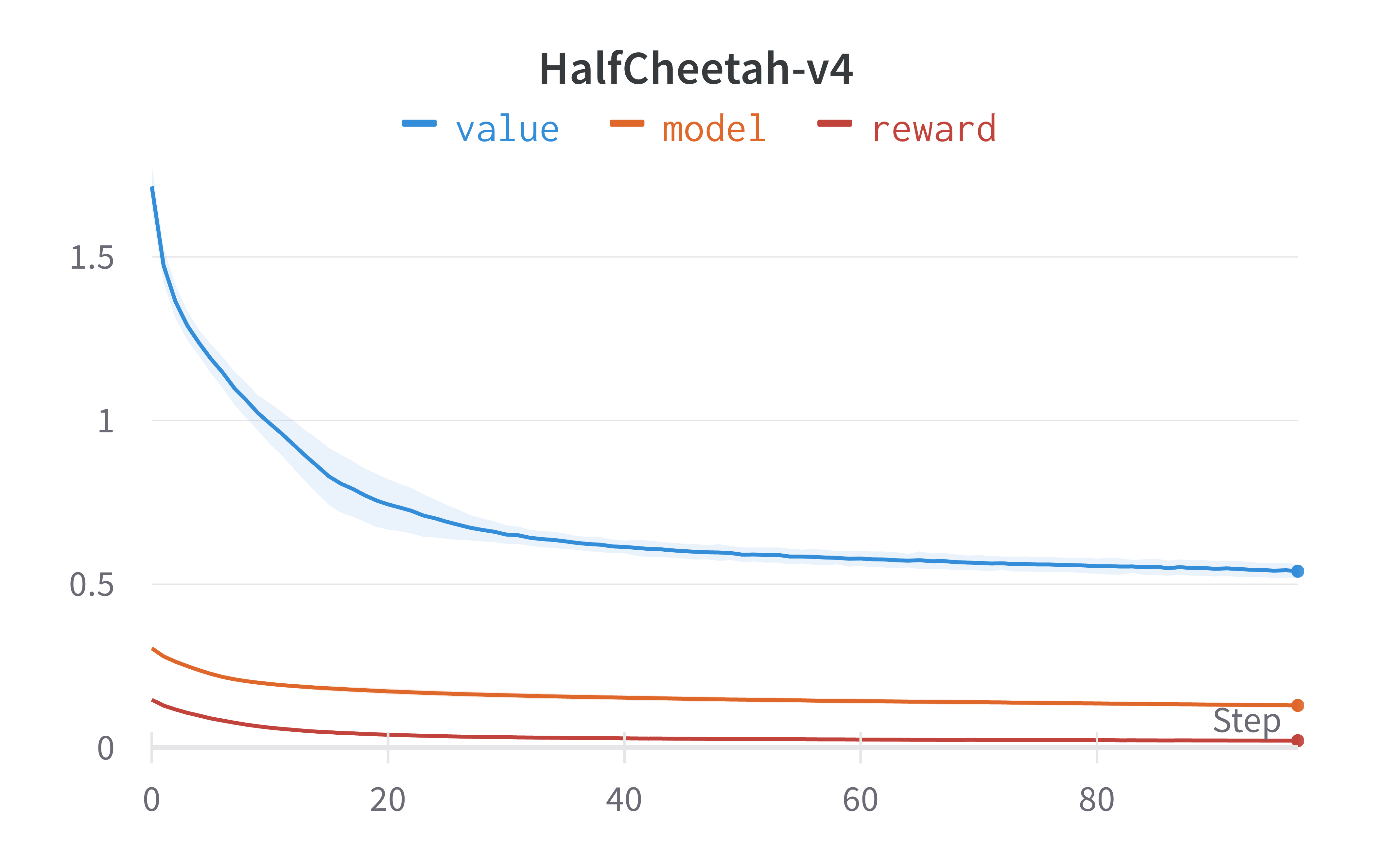
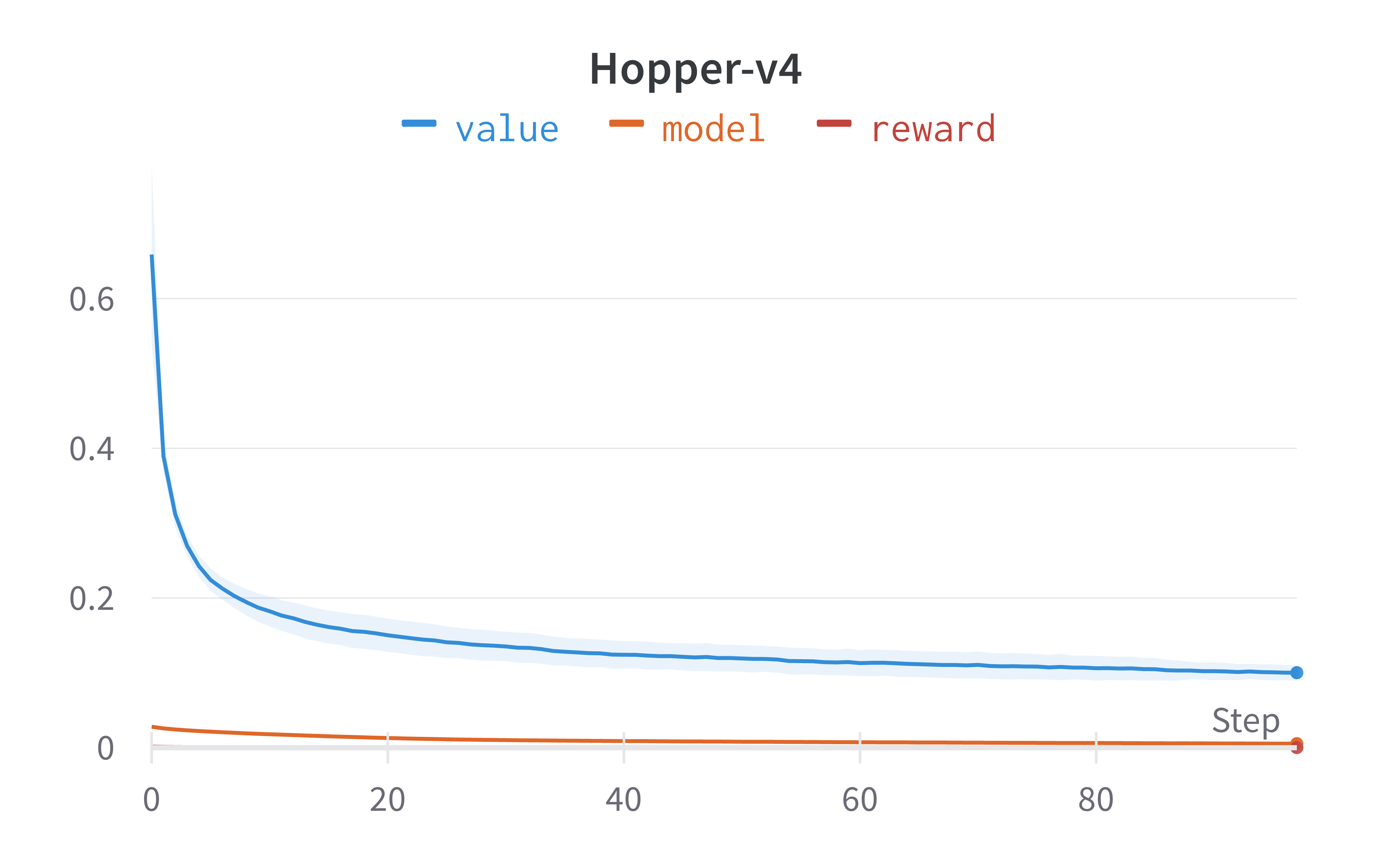
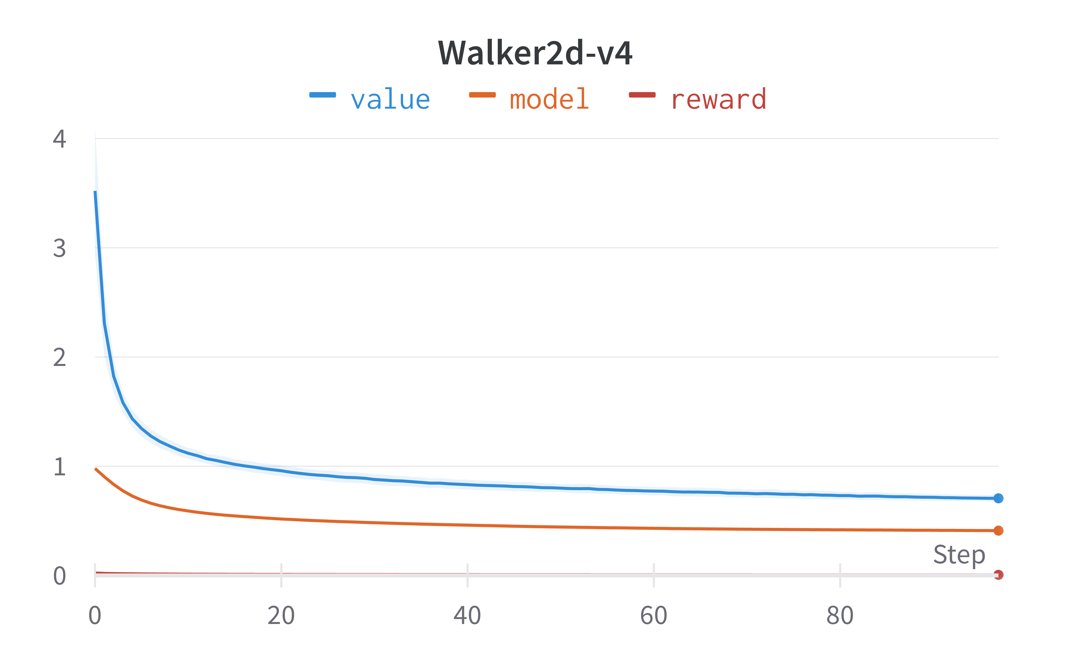
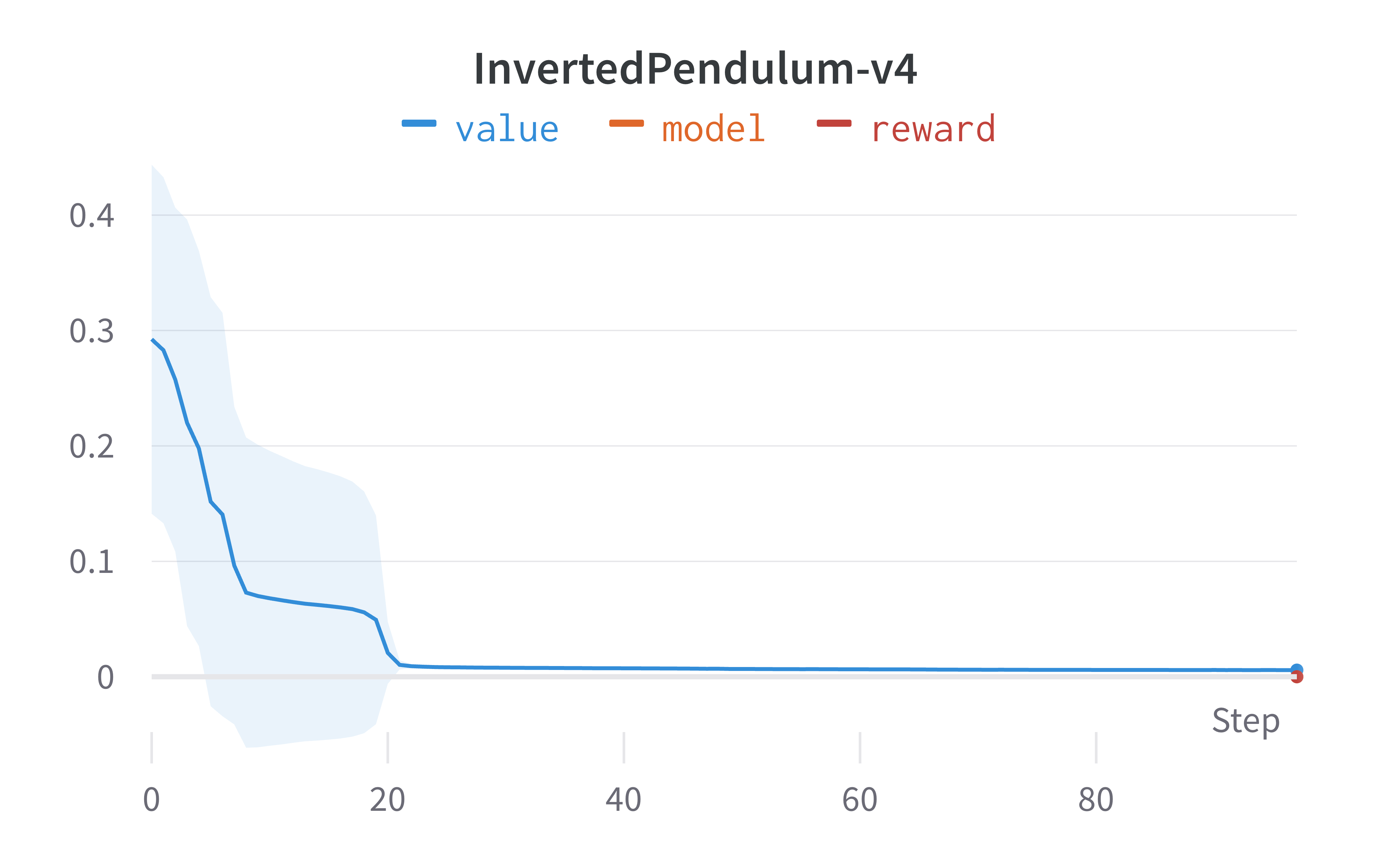
Figure 3: Approximation errors of the optimal $Q$-functions, reward functions, and transition functions in MuJoCo environments. In each environment, we run $5$ independent experiments and report the mean and standard deviation of the approximation errors.

For common MuJoCo Gym environments (Brockman et al., 2016), including Ant-v4, Hopper-v4, HalfCheetah-v4, InvertedPendulum-v4, and Walker2d-v4 , we find these objectives by training $d$-depth, $m$-width neural networks to fit the corresponding values over the trajectories generated by an SAC-trained agent.  In Figure 3, we visualize the approximation errors under $d=2,w=32$. Among the approximation objectives, the reward functions and the model transition functions are accessible, and we use Soft-Actor-Critic (Haarnoja et al., 2018) to learn the optimal $Q$-function. We observe a consistent phenomenon that the approximation errors of the optimal $Q$-function, in all environments, are much greater than the approximation errors of the transition and reward function. This finding concludes that in the above environments, the optimal $Q$-functions are more difficult to approximate than the transition functions and the reward function, which partly consolidate our hypothesis.

5 Conclusions

In this paper, we find that in a broad class of Markov Decision Processes, the transition function and the reward function can be computed by constant-depth, polynomial-sized circuits, whereas the optimal $Q$-function requires an exponential size for constant-depth circuits to compute. This separation reveals a rigorous gap in the representation complexity of the $Q$-function, the reward, and the transition function. Our experiments further corroborate that this gap is prevalent in common real-world environments.

Our theory lays the foundation of studying the representation complexity in RL and raises several open questions:

1. If we randomly sample an MDP, does the separation that the value function $\notin\mathbf{AC}^{0}$ and the reward and transition function $\in\mathbf{AC}^{0}$ occurs in high probability?

2. For $k\geq 1$, are there broad classes of MDPs such that the value function $\notin\mathbf{AC}^{k}$ and the reward and transition function $\in\mathbf{AC}^{k}$?

3. What are the typical circuit complexities of the value function, the reward function, and transition function?

Appendix A Supplementary Background on Circuit Complexity

Definition 9 (Majority).

For every $n\in\mathbb{Z}_{+}$, the $n$-variable majority function $\mathsf{MAJORITY}_{n}:\{0,1\}^{n}\to\{0,1\}$ is defined by $\mathsf{MAJORITY}_{n}(x_{1},\dots,x_{n})=\mathbbm{1}(\sum_{i=1}^{n}x_{i}>n/2)$. The majority function $\mathsf{MAJORITY}:\{0,1\}^{*}\to\{0,1\}$ is defined by

$$\mathsf{MAJORITY}(w):=\mathsf{MAJORITY}_{|w|}(w),~{}\forall w\in\{0,1\}^{*}.$$

Proposition A.1 (Razborov [1987], Smolensky [1987, 1993]).

$\mathsf{MAJORITY}\notin\mathbf{AC}^{0}$.

We also introduce another function that can be represented by polynomial-size constant-depth circuits, contrary to the above two “hard” functions.

Definition 10 (Addition).

For every $n\in\mathbb{Z}_{+}$, the length-$n$ integer addition function $\mathsf{ADDITION}_{n}:\{0,1\}^{n}\times\{0,1\}^{n}\to\{0,1\}^{n+1}$ is defined as follows: for any two binary strings $a_{1},a_{2}\in\{0,1\}^{n}$, the value $\mathsf{ADDITION}_{n}(a_{1},a_{2})$ is the $(n+1)$-bits binary representation of $a_{1}+a_{2}$. The integer addition function $\mathsf{ADDITION}:\{0,1\}^{*}\to\{0,1\}^{*}$ is defined by

$$\mathsf{ADDITION}(w_{1},w_{2}):=\mathsf{ADDITION}_{\max\{|w_{1}|,|w_{2}|\}}(w_{1},w_{2}),~{}\forall w_{1},w_{2}\in\{0,1\}^{*}.$$

Proposition A.2 (Proposition 1.15, Vollmer [1999]).

$\mathsf{ADDITION}\in\mathbf{AC}^{0}$.

Definition 11 (Maximum).

For every $n\in\mathbb{Z}_{+}$, the length-$n$ maximum function $\mathsf{MAX}_{n}:\{0,1\}^{n}\times\{0,1\}^{n}\to\{0,1\}^{n}$ is defined as follows: for any two binary strings $a_{1},a_{2}\in\{0,1\}^{n}$, the value $\mathsf{MAX}_{n}(a_{1},a_{2})$ is the $n$-bits binary representation of $\max\{a_{1},a_{2}\}$. The maximum function $\mathsf{MAX}:\{0,1\}^{*}\to\{0,1\}^{*}$ is defined by

$$\mathsf{MAX}(w_{1},w_{2}):=\mathsf{MAX}_{\max\{|w_{1}|,|w_{2}|\}}(w_{1},w_{2}),~{}\forall w_{1},w_{2}\in\{0,1\}^{*}.$$

Proposition A.3.

$\mathsf{MAX}\in\mathbf{AC}^{0}$.

Proof of Proposition A.3.

Fix any $n\in\mathbb{Z}_{+}$, and assume $w_{1},w_{2}\in\{0,1\}^{n}$. Let

$$k=\bigvee_{i=1}^{n}\left((w_{1})_{i}\wedge\neg(w_{2})_{i}\wedge\left(\bigwedge_{j=1}^{i-1}\neg((w_{1})_{j}\oplus(w_{2})_{j})\right)\right).$$

Therefore, $k=\mathbbm{1}(w_{1}>w_{2})$. Let the $i$-th bit of output be

$$((w_{1})_{i}\wedge k)\vee((w_{2})_{i}\wedge\neg k),$$

which is exact the $i$-th bit of $\max\{w_{1},w_{2}\}$. This circuit has polynomial size and constant depth, which completes the proof. ∎

Appendix B Proofs of Main Results

B.1 Useful results

We will use the following results frequently in the proofs.

Claim B.1.

If $C_{0},C_{1},\dots,C_{n}$ are circuits with polynomial (in $n$) size and constant depth, where $C_{i}$ has $k_{i}$ outputs for each $i\in[n]$ and $C_{0}$ has $\sum_{i=1}^{n}k_{i}$ inputs, then the circuit

$$C_{0}\left(C_{1}(x_{1}),\dots,C_{n}(x_{n})\right)$$

also has polynomial (in $n$) size and constant depth.

Claim B.2.

The XOR gate can be computed by a circuit with constant size.

Claim B.3.

For any integer $k=\operatorname{poly}(n)$, the gate $\delta(x_{1},\dots,x_{n})=\mathbbm{1}\left(k=\sum_{i=1}^{n}2^{n-i}\cdot x_{i}\right)$ can be computed by a circuit with polynomial size and constant depth.

B.2 Proof of Theorem 1

We need the following lemma.

Lemma 1 (Property of value function in unconditioned Majority MDPs).

In an unconditioned $n$-bits majority MDP with reward state $s_{\mathrm{reward}}$ and control function $f$, the value function $V^{*}$ (at time step $t=0$) over $\{s\in\{0,1\}^{b+n}:s[c]=\mathbf{0}_{b}\}$ is given by the following:

$$V^{*}(s)=n-\sum_{i=1}^{n}(\neg(s_{b+i}\oplus s_{\mathrm{reward},i}))+1.$$

Proof.

To find $V^{*}(s)$, it suffices to count the number of time steps an optimal agent takes to reach the reward state $(\mathbf{1}_{b},s_{\mathrm{reward}})$.

For the control bits to traverse from $\mathbf{0}_{b}$ to $\mathbf{1}_{b}$, it takes $2^{b}-1$ time steps. Indeed, by Definition 7, $f^{(i)}(\mathbf{0}_{b})\neq\mathbf{1}_{b}$ for any $i<2^{b}-1$ and $f^{(2^{b}-1)}(\mathbf{0}_{b})=\mathbf{1}_{b}$ (otherwise, $\left|\left\{f^{(k)}(\mathbf{0}_{b}):k=1,2,\dots,2^{b}-1\right\}\right|<2^{b}-1$ and as a result $\left\{f^{(k)}(\mathbf{0}_{b}):k=1,2,\dots,2^{b}-1\right\}$ can not traverse $\{0,1\}^{b}\backslash\{\mathbf{0}_{b}\}$). Thus, this corresponds to at least $2^{b}-1$ time steps in which action $a=0$ is played.

For the representation bits, starting from $s[r]$, reaching $s_{\mathrm{reward}}$ takes at least

$$\sum_{i=1}^{n}(\neg(s_{b+i}\oplus s_{\mathrm{reward},i}))$$

number of flipping, because each index $i$ such that $s_{b+i}\neq s_{\mathrm{reward},i}$ needs to be flipped. This corresponds to at least $\sum_{i=1}^{n}(\neg(s_{b+i}\oplus s_{\mathrm{reward},i}))$ time steps in which action $a=1$ is played.

In total, the agent needs to take at least $2^{b}+\sum_{i=1}^{n}(\neg(s_{b+i}\oplus s_{\mathrm{reward},i}))-1$ times steps before it can receive positive rewards. Since there are $2^{b}+n$ time steps in total, it follows that the agent gets a positive reward in at most $n-\sum_{i=1}^{n}(\neg(s_{b+i}\oplus s_{\mathrm{reward},i}))+1$ time steps. As a consequence,

$$V^{*}(s)\leq n-\sum_{i=1}^{n}(\neg(s_{b+i}\oplus s_{\mathrm{reward},i}))+1$$

On the other hand, consider the following policy:

$$\pi^{*}(s)=\begin{cases}1,&~{}\text{if}~{}s_{b+i}\neq s_{\mathrm{reward},i},~{}\text{where}~{}i=\sum_{j=1}^{b}2^{b-j}\cdot s_{j}\\ 0,&~{}\text{otherwise}.\end{cases}$$

This policy reaches the reward state in $2^{b}+\sum_{i=1}^{n}(\neg(s_{b+i}\oplus s_{\mathrm{reward},i}))-1$ time steps. Indeed, the control bits takes $2^{b}-1$ times steps to reach $\mathbf{1}_{b}$. During these time steps, the control bits (as a binary number) traverses $0,\dots,2^{b}-1$. Thus for any $i\in[n]$ such that $s_{b+i}\neq s_{\mathrm{reward},i}$, there exists a time $t$ such that the control bits at this time $t$ (as a binary number) equals $i$, and at this time step, the agent flipped the $i$-th coordinate of the representation bits by playing action $1$. Therefore, the representation bits takes $\sum_{i=1}^{n}(\neg(s_{b+i}\oplus s_{\mathrm{reward},i}))$ times steps to reach $s_{\mathrm{reward}}$. Combining, the agent arrives the state $(\mathbf{0}_{b},s_{\mathrm{reward}})$ after $2^{b}+\sum_{i=1}^{n}(\neg(s_{b+i}\oplus s_{\mathrm{reward},i}))-1$ time steps, and then collects reward $1$ in each of the remaining $n-\sum_{i=1}^{n}(\neg(s_{b+i}\oplus s_{\mathrm{reward},i}))+1$ time steps, resulting in a value of

$$V^{*}(s)=n-\sum_{i=1}^{n}(\neg(s_{b+i}\oplus s_{\mathrm{reward},i}))+1.$$

∎

Lemma 2.

Any control function can be computed by a constant depth, polynomial sized (in $n$) circuit.

Proof.

By Claim 2.13 in Arora and Barak [2009], any Boolean function can be computed by a CNF formula, i.e., Boolean circuits of the form

$$\bigwedge_{i=1}^{n}\left(\bigvee_{j=1}^{k_{i}}X_{i,j}\right).$$

As result, the control function can be computed by a depth-$2$, $2^{b}=\operatorname{poly}(n)$ sized circuit. ∎

Now we return to the proof of Theorem 1.

Proof.

First, we show that the model transition function can be computed by circuits with polynomial size and constant depth. Consider the following circuit:

$$C_{\mathrm{model}}(s,a)=\left(g(s_{1},\dots,s_{b},a),\left(s_{b+k}\oplus\left(\delta_{k}(s_{1},\dots,s_{b})\wedge a\right)\right)_{k=1}^{n}\right)$$

where $\oplus$ is the XOR gate, $g:\{0,1\}^{b+1}\to\{0,1\}^{b}$ such that $g(x_{1},\dots,x_{b},a)_{i}=(f(x_{1},\dots,x_{b})_{i}\wedge\neg a)\vee(x_{i}\wedge a)$ for all $i\in[b]$, and $\delta_{k}(x_{1},\dots,x_{b})=\mathbbm{1}(k=\sum_{j=1}^{b}2^{b-j}\cdot x_{j})$. We can verify that $C_{\mathrm{model}}=\mathbb{T}$. By Claim B.2, Claim B.3, and Lemma 2, the XOR gate, the control function $f$, and the gate $\delta_{k}$ can all be implemented by binary circuits with polynomial size and constant depth. As a result of Claim B.1, $C_{\mathrm{model}}$ also has polynomial size and constant depth.

Now, the reward function can be computed by the following simple circuit:

$$C_{\mathrm{reward}}(s)=s_{1}\wedge\dots\wedge s_{b}\wedge(\neg(s_{b+1}\oplus s_{\mathrm{reward},1}))\wedge\cdots\wedge(\neg(s_{b+n}\oplus s_{\mathrm{reward},n})).$$

Finally, we show that the value function can not be computed by a circuit with constant depth and polynomial size. By Lemma 1, we have

$$n+1-V^{*}(s)=\sum_{i=1}^{n}(\neg(s_{b+i}\oplus s_{\mathrm{reward},i}))\in\{0\}\cup[n]=\{0\}\cup[2^{b}-1],$$

which can be represented in binary form with $b$ bits. Therefore, the first (most significant) bit of $n+1-V^{*}(s)$ is the majority function of $\left(\neg(s_{b+i}\oplus s_{\mathrm{reward},i})\right)_{i=1}^{n}$. If there exists a circuit $C_{\mathrm{value}}=V^{*}$ with polynomial size and constant depth, then the circuit defined by

$$C_{\mathsf{MAJORITY}}(x_{1},\dots,x_{n})=n+1-C_{\mathrm{value}}\left(\mathbf{0}_{b},\neg x_{1}\oplus s_{\mathrm{reward},1},\dots,\neg x_{n}\oplus s_{\mathrm{reward},n}\right)$$

outputs the majority function in the first bit. By Proposition A.2, $C_{\mathsf{MAJORITY}}$ also has polynomial size and constant depth, which contradicts Proposition 2. This means that $V^{*}$ can not be computed by circuits with polynomial size and constant depth. Notice that $V^{*}(s)=\max_{a\in\mathcal{A}}Q^{*}(s,a)=\max\{Q^{*}(s,0),Q^{*}(s,1)\}$. By Proposition A.3 and Claim B.1, we conclude that the optimal $Q$-function can not be computed by circuits with polynomial size and constant depth. ∎

B.3 Proof of Theorem 2

We need the following lemmata.

Lemma 3.

With probability at least $1-e^{-\Omega(m)}$, there exists a set $A\subset[n]$ such that $|A|\geq n/2$ and $C(x)=1$ holds for any binary string $x\in\{0,1\}^{n}$ satisfying $x_{i}=s_{\mathrm{reward},i},\forall i\notin A$.

Proof.

It suffices to show that $C(s_{\mathrm{reward}})=1$ with at least $1-e^{-\Omega(m)}$. Indeed, in this case, since $m<n/2$, $C$ is independent on at least $n/2$ of the variables $x_{1},\dots,x_{n}$. The indices of such variables form the set $A$ that we are looking for.

To show that $C(s_{\mathrm{reward}})=1$ with at least $1-e^{-\Omega(m)}$, we assume WLOG that

$$C(x_{1},\dots,x_{n})=\bigvee_{i=1}^{n}\left(\bigwedge_{j=1}^{k_{i}}X_{i,j}\right)$$

where $X_{i,j}=x_{l}$ or $X_{i,j}=\neg x_{l}$ for some $l\in[m]$. Notice

$$\mathbb{P}\left(\left(\bigwedge_{j=1}^{k_{i}}X_{i,j}\right)=1\right)=2^{-k_{i}}=\Omega(1)$$

since each $X_{i,j}$ is sampled i.i.d. from $\{x_{l},\neg x_{l}\}_{l\in[m]}$ uniformly at random. It follows that

$$\mathbb{P}\left(C(x_{1},\dots,x_{n})=1\right)= ~{}1-\prod_{i=1}^{n}\mathbb{P}\left(\left(\bigwedge_{j=1}^{k_{i}}X_{i,j}\right)=0\right)$$

$$= ~{}1-\prod_{i=1}^{n}(1-2^{-k_{i}})$$

$$\geq ~{}1-e^{-\Omega(m)}.$$

∎

Lemma 4 (Property of value function in conditioned Majority MDPs).

In an $n$-bits majority MDP with reward state $s_{\mathrm{reward}}$, control function $f$ and condition $C$, if there exists a set $A\subset[n]$ such that $|A|=\lceil n/2\rceil=2^{b-1}-1$ and $C(x)=1$ holds for any binary string $x\in\{0,1\}^{n}$ satisfying $x_{i}=s_{\mathrm{reward},i},\forall i\notin A$, then the value function $V^{*}$ over $\{s\in\{0,1\}^{b+n}:s[c]=\mathbf{0}_{b},s_{b+i}=s_{\mathrm{reward},i}~{}(\forall i\notin A)\}$ is given by the following:

$$V^{*}(s)=n-\sum_{i\in A}(\neg(s_{b+i}\oplus s_{\mathrm{reward},i}))+1.$$

Proof.

To find $V^{*}(s)$, it suffices to count the number of actions it takes to reach the reward state $(\mathbf{1}_{b},s_{\mathrm{reward}})$.

For the control bits to travel from $\mathbf{0}_{b}$ to $\mathbf{1}_{b}$, it takes $2^{b}-1$ time steps. Indeed, by Definition 7, $f^{(i)}(\mathbf{0}_{b})\neq\mathbf{1}_{b}$ for any $i<2^{b}-1$ and $f^{(2^{b}-1)}(\mathbf{0}_{b})\neq\mathbf{1}_{b}$ (otherwise, $\left|\left\{f^{(k)}(\mathbf{0}_{b}):k=1,2,\dots,2^{b}-1\right\}\right|<2^{b}-1$ and as a result $\left\{f^{(k)}(\mathbf{0}_{b}):k=1,2,\dots,2^{b}-1\right\}$ can not traverse $\{0,1\}^{b}\backslash\{\mathbf{0}_{b}\}$). Thus, this corresponds to at least $2^{b}-1$ time steps in which action $a=0$ is played.

For the representation bits, starting from $s[r]$, reaching $s_{\mathrm{reward}}$ takes at least

$$\sum_{i\in A}(\neg(s_{b+i}\oplus s_{\mathrm{reward},i}))$$

number of flipping, as each index $i$ such that $s_{b+i}\neq s_{\mathrm{reward},i}$ needs to be flipped. This corresponds to at least $\sum_{i\in A}(\neg(s_{b+i}\oplus s_{\mathrm{reward},i}))$ time steps in which action $a=1$ is played.

In total, the agent needs to take at least $2^{b}+\sum_{i\in A}(\neg(s_{b+i}\oplus s_{\mathrm{reward},i}))-1$ times steps before it can receive positive rewards. Since there are $2^{b}+n$ time step in total, it follows that the agent gets positive reward in at most $n-\sum_{i\in A}(\neg(s_{b+i}\oplus s_{\mathrm{reward},i}))+1$ time steps. As a consequence,

$$V^{*}(s)\leq n-\sum_{i\in A}(\neg(s_{b+i}\oplus s_{\mathrm{reward},i}))+1$$

On the other hand, consider the following policy:

$$\pi^{*}(s)=\begin{cases}1,&~{}\text{if}~{}s_{b+i}\neq s_{\mathrm{reward},i},~{}\text{where}~{}i=\sum_{j=1}^{b}2^{b-j}\cdot s_{j}\\ 0,&~{}\text{otherwise}.\end{cases}$$

This policy reaches the reward state in $2^{b}+\sum_{i\in A}(\neg(s_{b+i}\oplus s_{\mathrm{reward},i}))-1$ time steps. Indeed, the control bits takes $2^{b}-1$ times steps to reach $\mathbf{1}_{b}$. During these time steps, the control bits (as a binary number) traverses $0,\dots,2^{b}-1$. Thus for any $i\in[n]$ such that $s_{b+i}\neq s_{\mathrm{reward},i}$, there exists a time $t$ such that the control bits at this time $t$ (as a binary number) equals $i$, and at this time step, the agent flipped the $i$-th coordinate of the representation bits by playing action $1$ (note that the flipping operation can always be applied since the condition is always satisfied under the current policy). Therefore, the representation bits takes $\sum_{i\in A}(\neg(s_{b+i}\oplus s_{\mathrm{reward},i}))$ times steps to reach $s_{\mathrm{reward}}$. Combining, the agent arrives the state $(\mathbf{0}_{b},s_{\mathrm{reward}})$ after $2^{b}+\sum_{i\in A}(\neg(s_{b+i}\oplus s_{\mathrm{reward},i}))-1$ time steps, and then collects reward $1$ in each of the remaining $n-\sum_{i\in A}(\neg(s_{b+i}\oplus s_{\mathrm{reward},i}))+1$ time steps, resulting in a value of

$$V^{*}(s)=n-\sum_{i\in A}(\neg(s_{b+i}\oplus s_{\mathrm{reward},i}))+1.$$

∎

Now we return to the proof of Theorem 2.

Proof.

First, we show that the model function can be computed by circuits with polynomial size and constant depth. Consider the following circuit:

$$C_{\mathrm{model}}(s,a)=\left(g(s_{1},\dots,s_{b}),\left(s_{b+k}\oplus\left(\delta_{k}(s_{1},\dots,s_{b})\wedge a\wedge C(s[r])\right)\right)_{k=1}^{n}\right)$$

where $\oplus$ is the XOR gate, $g:\{0,1\}^{b+1}\to\{0,1\}^{b}$ such that $g(x_{1},\dots,x_{b},a)_{i}=(f(x_{1},\dots,x_{b})_{i}\wedge\neg a)\vee(x_{i}\wedge a)$ for all $i\in[b]$, and $\delta_{k}(x_{1},\dots,x_{b})=\mathbbm{1}(k=\sum_{j=1}^{b}2^{b-j}\cdot x_{j})$. We can verify that $C_{\mathrm{model}}=\mathbb{T}$. By Claim B.2, Claim B.3, and Lemma 2, the XOR gate, the control function $f$, the function $C(s[r])$, and the gate $\delta_{k}$ can all be implemented by binary circuits with polynomial size and constant depth. As a result of Claim B.1, $C_{\mathrm{model}}$ also has polynomial size and constant depth.

Now, the reward function can be computed by the following simple circuit:

$$C_{\mathrm{reward}}(s)=s_{1}\wedge\dots\wedge s_{b}\wedge(\neg(s_{b+1}\oplus s_{\mathrm{reward},1}))\wedge\cdots\wedge(\neg(s_{b+n}\oplus s_{\mathrm{reward},n})).$$

Finally, we show that with high probability, the value function can not be computed by a circuit with constant depth and polynomial size. By Lemma 3, with probability at least $1-e^{-\Omega(m)}$, there exists a set $A\subset[n]$ such that $|A|\geq n/2$ and $C(x)=1$ holds for any binary string $x\in\{0,1\}^{n}$ satisfying $x_{i}=s_{\mathrm{reward},i},\forall i\notin A$. We can reduce the size of $A$ by deleting some elements to make $|A|=\lceil n/2\rceil=2^{b-1}-1$ and the above property still holds. Denote $A=\{a(1)<\dots<a(L)\}$ where $a:[L]\to[n]$. Define $h:\{0,1\}^{L}\to\{0,1\}^{b}$

$$h\left((x_{1},\dots,x_{L})\right)=n+1-V^{*}\left((\mathbf{0}_{b},s^{\prime})\right),~{}\text{where}~{}s^{\prime}_{j}=\begin{cases}s_{\mathrm{reward},j},&~{}j\notin A\\ \neg x_{a^{-1}(j)}\oplus s_{\mathrm{reward},j},&~{}j\in A\end{cases}.$$

Due to Lemma 4, $h\left(x\right)$ can be represented in binary form with $(b-1)$ bits, and the first (most significant) bit of $h(x)$ is the majority function of $x$. If there exists a circuit $C_{\mathrm{value}}=V^{*}$ with polynomial size and constant depth, then the circuit defined by

$$C_{\mathsf{MAJORITY}}(x_{1},\dots,x_{L})=n+1-C_{\mathrm{value}}\left(\mathbf{0}_{b},\neg x_{a^{-1}(1)}\oplus s_{\mathrm{reward},1},\dots,\neg x_{a^{-1}(n)}\oplus s_{\mathrm{reward},n}\right)$$

where $a^{-1}(i)=i$ if $i\notin A$, outputs $h$. By Proposition A.2, $C_{\mathsf{MAJORITY}}$ also has polynomial size and constant depth, which contradicts Proposition A.1. This means that $V^{*}$ can not be computed by circuits with polynomial size and constant depth. Notice that $V^{*}(s)=\max_{a\in\mathcal{A}}Q^{*}(s,a)=\max\{Q^{*}(s,0),Q^{*}(s,1)\}$. By Proposition A.3 and Claim B.1, we conclude that the optimal $Q$-function can not be computed by circuits with polynomial size and constant depth. ∎

Appendix C Experiment Details

Table 1 shows the parameters used in SAC training to learn the optimal $Q$-function. Table 2 shows parameters for fitting neural networks to the value, reward, and transition functions.

Hyperparameter	Value(s)
Optimizer	Adam [Kingma and Ba, 2014]
Learning Rate	0.0003
Batch Size	1000
Number of Epochs	100000
Init_temperature	0.1
Episode length	1000
Discount factor	0.99
number of hidden layers (all networks)	256
number of hidden units per layer	2
target update interval	1

Table 1: Hyperparameters in Soft-Actor-Critic

Hyperparameter	Value(s)
Optimizer	Adam [Kingma and Ba, 2014]
Learning Rate	0.001
Batch Size	32
Number of Epochs	100

Table 2: Hyperparameters of fitting neural networks to the value, reward, and transition functions

References

- Agarwal et al. [2019] Alekh Agarwal, Nan Jiang, Sham M Kakade, and Wen Sun. Reinforcement learning: Theory and algorithms. CS Dept., UW Seattle, Seattle, WA, USA, Tech. Rep, 2019.
- Agarwal et al. [2020] Alekh Agarwal, Sham M Kakade, Jason D Lee, and Gaurav Mahajan. Optimality and approximation with policy gradient methods in Markov decision processes. In Conference on Learning Theory, pages 64–66. PMLR, 2020.
- Arora and Barak [2009] Sanjeev Arora and Boaz Barak. Computational complexity: a modern approach. Cambridge University Press, 2009.
- Auer et al. [2008] Peter Auer, Thomas Jaksch, and Ronald Ortner. Near-optimal regret bounds for reinforcement learning. Advances in neural information processing systems, 21, 2008.
- Azar et al. [2017] Mohammad Gheshlaghi Azar, Ian Osband, and Rémi Munos. Minimax regret bounds for reinforcement learning. In Proceedings of the 34th International Conference on Machine Learning-Volume 70, pages 263–272. JMLR. org, 2017.
- Bao et al. [2014] Chenglong Bao, Qianxiao Li, Zuowei Shen, Cheng Tai, Lei Wu, and Xueshuang Xiang. Approximation analysis of convolutional neural networks. work, 65, 2014.
- Biewald [2020] Lukas Biewald. Experiment tracking with weights and biases. Software available from wandb.com, 2:233, 2020.
- Boppana and Sipser [1990] Ravi B Boppana and Michael Sipser. The complexity of finite functions. In Algorithms and complexity, pages 757–804. Elsevier, 1990.
- Brockman et al. [2016] Greg Brockman, Vicki Cheung, Ludwig Pettersson, Jonas Schneider, John Schulman, Jie Tang, and Wojciech Zaremba. Openai gym, 2016.
- Buckman et al. [2018] Jacob Buckman, Danijar Hafner, George Tucker, Eugene Brevdo, and Honglak Lee. Sample-efficient reinforcement learning with stochastic ensemble value expansion. Advances in neural information processing systems, 31, 2018.
- Chua et al. [2018] Kurtland Chua, Roberto Calandra, Rowan McAllister, and Sergey Levine. Deep reinforcement learning in a handful of trials using probabilistic dynamics models. Advances in neural information processing systems, 31, 2018.
- Clavera et al. [2018] Ignasi Clavera, Jonas Rothfuss, John Schulman, Yasuhiro Fujita, Tamim Asfour, and Pieter Abbeel. Model-based reinforcement learning via meta-policy optimization. In Conference on Robot Learning, pages 617–629. PMLR, 2018.
- Dean et al. [2018] Sarah Dean, Horia Mania, Nikolai Matni, Benjamin Recht, and Stephen Tu. Regret bounds for robust adaptive control of the linear quadratic regulator. Advances in Neural Information Processing Systems, 31, 2018.
- Dean et al. [2020] Sarah Dean, Horia Mania, Nikolai Matni, Benjamin Recht, and Stephen Tu. On the sample complexity of the linear quadratic regulator. Foundations of Computational Mathematics, 20(4):633–679, 2020.
- Dong et al. [2020a] Kefan Dong, Yuping Luo, and Tengyu Ma. On the expressivity of neural networks for deep reinforcement learning. In International Conference on Machine Learning (ICML), 2020a.
- Dong et al. [2020b] Kefan Dong, Yuping Luo, Tianhe Yu, Chelsea Finn, and Tengyu Ma. On the expressivity of neural networks for deep reinforcement learning. In International conference on machine learning, pages 2627–2637. PMLR, 2020b.
- Draeger et al. [1995] Andreas Draeger, Sebastian Engell, and Horst Ranke. Model predictive control using neural networks. IEEE Control Systems Magazine, 15(5):61–66, 1995.
- Du and Narasimhan [2019] Yilun Du and Karthic Narasimhan. Task-agnostic dynamics priors for deep reinforcement learning. In International Conference on Machine Learning, pages 1696–1705. PMLR, 2019.
- Feinberg et al. [2018] Vladimir Feinberg, Alvin Wan, Ion Stoica, Michael I Jordan, Joseph E Gonzalez, and Sergey Levine. Model-based value estimation for efficient model-free reinforcement learning. arXiv preprint arXiv:1803.00101, 2018.
- Furst et al. [1984] Merrick Furst, James B Saxe, and Michael Sipser. Parity, circuits, and the polynomial-time hierarchy. Mathematical systems theory, 17(1):13–27, 1984.
- Haarnoja et al. [2018] Tuomas Haarnoja, Aurick Zhou, Pieter Abbeel, and Sergey Levine. Soft actor-critic: Off-policy maximum entropy deep reinforcement learning with a stochastic actor. In International conference on machine learning, pages 1861–1870. PMLR, 2018.
- Hastad [1986] John Hastad. Almost optimal lower bounds for small depth circuits. In Proceedings of the eighteenth annual ACM symposium on Theory of computing, pages 6–20, 1986.
- Heess et al. [2015] Nicolas Heess, Gregory Wayne, David Silver, Timothy Lillicrap, Tom Erez, and Yuval Tassa. Learning continuous control policies by stochastic value gradients. Advances in neural information processing systems, 28, 2015.
- Huang et al. [2021] Baihe Huang, Kaixuan Huang, Sham Kakade, Jason D Lee, Qi Lei, Runzhe Wang, and Jiaqi Yang. Going beyond linear rl: Sample efficient neural function approximation. Advances in Neural Information Processing Systems, 34:8968–8983, 2021.
- Janner et al. [2019] Michael Janner, Justin Fu, Marvin Zhang, and Sergey Levine. When to trust your model: Model-based policy optimization. Advances in neural information processing systems, 32, 2019.
- Jin et al. [2018] Chi Jin, Zeyuan Allen-Zhu, Sebastien Bubeck, and Michael I Jordan. Is Q-learning provably efficient? In Advances in Neural Information Processing Systems, pages 4863–4873, 2018.
- Jin et al. [2019] Chi Jin, Zhuoran Yang, Zhaoran Wang, and Michael I Jordan. Provably efficient reinforcement learning with linear function approximation. arXiv preprint arXiv:1907.05388, 2019.
- Kakade [2003] SM Kakade. On the sample complexity of reinforcement learning. PhD thesis, University of London, 2003.
- Karp [1982] Richard Karp. Turing machines that take advice. Enseign. Math., 28:191–209, 1982.
- Kingma and Ba [2014] Diederik P Kingma and Jimmy Ba. Adam: A method for stochastic optimization. arXiv preprint arXiv:1412.6980, 2014.
- Kober et al. [2014] Jens Kober, Andrew Bagnell, and Jan Peters. Reinforcement learning in robotics: A survey. Springer Tracts in Advanced Robotics, 97:9–67, 2014.
- Leighton [2014] F Thomson Leighton. Introduction to parallel algorithms and architectures: Arrays· trees· hypercubes. Elsevier, 2014.
- Levine and Koltun [2013] Sergey Levine and Vladlen Koltun. Guided policy search. In International conference on machine learning, pages 1–9. PMLR, 2013.
- Lillicrap et al. [2015] Timothy P Lillicrap, Jonathan J Hunt, Alexander Pritzel, Nicolas Heess, Tom Erez, Yuval Tassa, David Silver, and Daan Wierstra. Continuous control with deep reinforcement learning. arXiv preprint arXiv:1509.02971, 2015.
- Lu et al. [2021] Jianfeng Lu, Zuowei Shen, Haizhao Yang, and Shijun Zhang. Deep network approximation for smooth functions. SIAM Journal on Mathematical Analysis, 53(5):5465–5506, 2021.
- Lu et al. [2017] Zhou Lu, Hongming Pu, Feicheng Wang, Zhiqiang Hu, and Liwei Wang. The expressive power of neural networks: A view from the width. Advances in neural information processing systems, 30, 2017.
- Luo et al. [2018] Yuping Luo, Huazhe Xu, Yuanzhi Li, Yuandong Tian, Trevor Darrell, and Tengyu Ma. Algorithmic framework for model-based deep reinforcement learning with theoretical guarantees. arXiv preprint arXiv:1807.03858, 2018.
- Mnih et al. [2013] Volodymyr Mnih, Koray Kavukcuoglu, David Silver, Alex Graves, Ioannis Antonoglou, Daan Wierstra, and Martin Riedmiller. Playing atari with deep reinforcement learning. arXiv preprint arXiv:1312.5602, 2013.
- Mnih et al. [2015] Volodymyr Mnih, Koray Kavukcuoglu, David Silver, Andrei A Rusu, Joel Veness, Marc G Bellemare, Alex Graves, Martin Riedmiller, Andreas K Fidjeland, Georg Ostrovski, et al. Human-level control through deep reinforcement learning. Nature, 518(7540):529–533, 2015.
- Moerland et al. [2023] Thomas M Moerland, Joost Broekens, Aske Plaat, Catholijn M Jonker, et al. Model-based reinforcement learning: A survey. Foundations and Trends® in Machine Learning, 16(1):1–118, 2023.
- Moravčík et al. [2017] Matej Moravčík, Martin Schmid, Neil Burch, Viliam Lisỳ, Dustin Morrill, Nolan Bard, Trevor Davis, Kevin Waugh, Michael Johanson, and Michael Bowling. Deepstack: Expert-level artificial intelligence in heads-up no-limit poker. Science, 356(6337):508–513, 2017.
- Nagabandi et al. [2018] Anusha Nagabandi, Gregory Kahn, Ronald S Fearing, and Sergey Levine. Neural network dynamics for model-based deep reinforcement learning with model-free fine-tuning. In 2018 IEEE international conference on robotics and automation (ICRA), pages 7559–7566. IEEE, 2018.
- Nagabandi et al. [2020] Anusha Nagabandi, Kurt Konolige, Sergey Levine, and Vikash Kumar. Deep dynamics models for learning dexterous manipulation. In Conference on Robot Learning, pages 1101–1112. PMLR, 2020.
- Oh et al. [2017] Junhyuk Oh, Satinder Singh, and Honglak Lee. Value prediction network. Advances in neural information processing systems, 30, 2017.
- Piché et al. [2018] Alexandre Piché, Valentin Thomas, Cyril Ibrahim, Yoshua Bengio, and Chris Pal. Probabilistic planning with sequential monte carlo methods. In International Conference on Learning Representations, 2018.
- Rajeswaran et al. [2016] Aravind Rajeswaran, Sarvjeet Ghotra, Balaraman Ravindran, and Sergey Levine. Epopt: Learning robust neural network policies using model ensembles. arXiv preprint arXiv:1610.01283, 2016.
- Rashidinejad et al. [2022] Paria Rashidinejad, Hanlin Zhu, Kunhe Yang, Stuart Russell, and Jiantao Jiao. Optimal conservative offline rl with general function approximation via augmented lagrangian. arXiv preprint arXiv:2211.00716, 2022.
- Rawlings [2000] James B Rawlings. Tutorial overview of model predictive control. IEEE control systems magazine, 20(3):38–52, 2000.
- Razborov [1987] Alexander A. Razborov. Lower bounds on the size of bounded depth circuits over a complete basis with logical addition. Mathematical notes of the Academy of Sciences of the USSR, 41:333–338, 1987. URL https://api.semanticscholar.org/CorpusID:121744639.
- Razborov [1989] Alexander A Razborov. On the method of approximations. In Proceedings of the twenty-first annual ACM symposium on Theory of computing, pages 167–176, 1989.
- Savage [1972] John E Savage. Computational work and time on finite machines. Journal of the ACM (JACM), 19(4):660–674, 1972.
- Shalev-Shwartz et al. [2016] Shai Shalev-Shwartz, Shaked Shammah, and Amnon Shashua. Safe, multi-agent, reinforcement learning for autonomous driving. arXiv preprint arXiv:1610.03295, 2016.
- Shannon [1949] Claude E Shannon. The synthesis of two-terminal switching circuits. The Bell System Technical Journal, 28(1):59–98, 1949.
- Silver et al. [2016] David Silver, Aja Huang, Chris J. Maddison, Arthur Guez, Laurent Sifre, George Van Den Driessche, Julian Schrittwieser, Ioannis Antonoglou, Veda Panneershelvam, and Marc Lanctot. Mastering the game of Go with deep neural networks and tree search. Nature, 529(7587):484, 2016.
- Silver et al. [2017] David Silver, Hado Hasselt, Matteo Hessel, Tom Schaul, Arthur Guez, Tim Harley, Gabriel Dulac-Arnold, David Reichert, Neil Rabinowitz, Andre Barreto, et al. The predictron: End-to-end learning and planning. In International Conference on Machine Learning, pages 3191–3199. PMLR, 2017.
- Singh et al. [2000] Satinder Singh, Tommi Jaakkola, Michael L Littman, and Csaba Szepesvári. Convergence results for single-step on-policy reinforcement-learning algorithms. Machine learning, 38:287–308, 2000.
- Smolensky [1987] Roman Smolensky. Algebraic methods in the theory of lower bounds for boolean circuit complexity. In Proceedings of the nineteenth annual ACM symposium on Theory of computing, pages 77–82, 1987.
- Smolensky [1993] Roman Smolensky. On representations by low-degree polynomials. In Proceedings of 1993 IEEE 34th Annual Foundations of Computer Science, pages 130–138. IEEE, 1993.
- Strehl et al. [2006] Alexander L Strehl, Lihong Li, Eric Wiewiora, John Langford, and Michael L Littman. PAC model-free reinforcement learning. In Proceedings of the 23rd international conference on Machine learning, pages 881–888, 2006.
- Sun et al. [2019] Wen Sun, Nan Jiang, Akshay Krishnamurthy, Alekh Agarwal, and John Langford. Model-based rl in contextual decision processes: Pac bounds and exponential improvements over model-free approaches. In Conference on learning theory, pages 2898–2933. PMLR, 2019.
- Trakhtenbrot [1984] Boris A Trakhtenbrot. A survey of russian approaches to perebor (brute-force searches) algorithms. Annals of the History of Computing, 6(4):384–400, 1984.
- Tu and Recht [2018] Stephen Tu and Benjamin Recht. The gap between model-based and model-free methods on the linear quadratic regulator: An asymptotic viewpoint. arXiv preprint arXiv:1812.03565, 2018.
- Tu and Recht [2019] Stephen Tu and Benjamin Recht. The gap between model-based and model-free methods on the linear quadratic regulator: An asymptotic viewpoint. In Conference on Learning Theory, pages 3036–3083, 2019.
- Valiant [1975] Leslie G Valiant. On non-linear lower bounds in computational complexity. In Proceedings of the seventh annual ACM symposium on Theory of computing, pages 45–53, 1975.
- Van Hasselt et al. [2016] Hado Van Hasselt, Arthur Guez, and David Silver. Deep reinforcement learning with double q-learning. In Proceedings of the AAAI conference on artificial intelligence, volume 30, 2016.
- Vollmer [1999] Heribert Vollmer. Introduction to circuit complexity: a uniform approach. Springer Science & Business Media, 1999.
- Wang et al. [2020] Ruosong Wang, Ruslan Salakhutdinov, and Lin F Yang. Provably efficient reinforcement learning with general value function approximation. arXiv preprint arXiv:2005.10804, 2020.
- Wang and Ba [2019] Tingwu Wang and Jimmy Ba. Exploring model-based planning with policy networks. arXiv preprint arXiv:1906.08649, 2019.
- Weber et al. [2017] Théophane Weber, Sébastien Racaniere, David P Reichert, Lars Buesing, Arthur Guez, Danilo Jimenez Rezende, Adria Puigdomenech Badia, Oriol Vinyals, Nicolas Heess, Yujia Li, et al. Imagination-augmented agents for deep reinforcement learning. arXiv preprint arXiv:1707.06203, 2017.
- Yu et al. [2020] Chao Yu, Jiming Liu, and Shamim Nemati. Reinforcement learning in healthcare: A survey. In arXiv preprint arXiv:1908.08796, 2020.
- Yurtsever et al. [2020] Ekim Yurtsever, Jacob Lambert, Alexander Carballo, and Kazuya Takeda. A survey of autonomous driving: Common practices and emerging technologies. IEEE access, 8:58443–58469, 2020.
- Zanette and Brunskill [2019] Andrea Zanette and Emma Brunskill. Tighter problem-dependent regret bounds in reinforcement learning without domain knowledge using value function bounds, 2019.
- Zhan et al. [2023] Wenhao Zhan, Shicong Cen, Baihe Huang, Yuxin Chen, Jason D Lee, and Yuejie Chi. Policy mirror descent for regularized reinforcement learning: A generalized framework with linear convergence. SIAM Journal on Optimization, 33(2):1061–1091, 2023.
- Zhu and Zhang [2023] Hanlin Zhu and Amy Zhang. Provably efficient offline goal-conditioned reinforcement learning with general function approximation and single-policy concentrability, 2023.
- Zhu et al. [2023a] Hanlin Zhu, Paria Rashidinejad, and Jiantao Jiao. Importance weighted actor-critic for optimal conservative offline reinforcement learning. arXiv preprint arXiv:2301.12714, 2023a.
- Zhu et al. [2023b] Hanlin Zhu, Ruosong Wang, and Jason Lee. Provably efficient reinforcement learning via surprise bound. In International Conference on Artificial Intelligence and Statistics, pages 4006–4032. PMLR, 2023b.