Quantum Entanglement Phase Transitions and Computational Complexity: Insights from Ising Models

Abstract

In this paper, we construct 2-dimensional bipartite cluster states and perform single-qubit measurements on the bulk qubits. We explore the entanglement scaling of the unmeasured 1-dimensional boundary state and show that under certain conditions, the boundary state can undergo a volume-law to an area-law entanglement transition driven by variations in the measurement angle. We bridge this boundary state entanglement transition and the measurement-induced phase transition in the non-unitary 1+1-dimensional circuit via the transfer matrix method. We also explore the application of this entanglement transition on the computational complexity problems. Specifically, we establish a relation between the boundary state entanglement transition and the sampling complexity of the bipartite $2$d cluster state, which is directly related to the computational complexity of the corresponding Ising partition function with complex parameters. By examining the boundary state entanglement scaling, we numerically identify the parameter regime for which the $2$d quantum state can be efficiently sampled, which indicates that the Ising partition function can be evaluated efficiently in such a region.

I Introduction

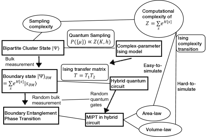
Figure 1: Road map of this work

.

Measurement-induced phase transitions (MIPT) occurring within monitored quantum systems have garnered significant attention, inspiring extensive research to unravel their profound implications. Numerous studies have explored these transitions in various quantum systems, investigating their fundamental properties and experimental realization [1, 2, 3, 4, 5, 6, 7, 8, 9, 10, 11, 12, 13, 14, 15, 16, 17, 18]. One type of phase transition exists in the hybrid quantum circuit composed of entangling unitary gates and disentangling measurements. An entanglement transition manifests by tuning the measurement rate, transitioning from a volume-law phase to an area-law phase [1, 2, 3, 4, 7, 8, 6, 5, 9]. Another example of entanglement phase transitions occurs in measurement-only circuits, where the transition is between different area-law phases, with a deviation from area-law scaling at the critical point [13, 12, 14, 15, 17, 16, 18]. An illustrative example of such a system is the $ZZ/X$ competing measurement model in [17], whose transition can be understood in classical percolation.

MIPT in the 1+1D hybrid quantum circuit naturally implies a complexity phase transition regarding simulability. The entanglement structure of a quantum system plays a crucial role in determining the computational difficulty of simulating the system on a classical computer. Simulating a volume-law entangled system is widely recognized as challenging due to the exponential resources required to store the quantum state. Conversely, an area-law entangled system is easily simulatable, as demonstrated by the matrix product state (MPS) representation and tensor networks, along with their variants [19]. The volume-law to area-law entanglement phase transition thus indicates a transition between phases that are hard to simulate classically to phases that are easy to simulate.

Moreover, MIPT is closely related to other computational challenges. In the context of the Random Circuit Sampling (RCS) problem, which is commonly employed to assess quantum advantage [20], classical simulation is believed to be computationally arduous [21, 22]. Recent findings [23] indicate that for RCS with a finite depth $d$, approximate sampling becomes viable for circuits with depths up to $d_{c}$, a finite critical depth. Conversely, approximating the outcomes becomes computationally demanding when the circuit depth exceeds $d_{c}$. The complexity of this sampling problem can be understood by treating one spatial dimension as the time axis and interpreting circuit depth as the inverse of the measurement rate $p=1/d$ in a hybrid circuit. As a result, a connection emerges between the challenge of approximating outputs in shallow 2D circuits and the transition from a 1+1D volume law to an area-law entanglement phase. Recent research on MIPT in shallow circuits also suggests the existence of entanglement phase transitions induced by measurements on 2D quantum states prepared by shallow circuits [24, 25].

Motivated by these advancements, in our recent work [24], we explicitly consider 2D quantum states generated by various Clifford shallow circuits. We then investigate the entanglement structure of the boundary 1D quantum state after measuring all the bulk qubits. Remarkably, we demonstrate that this boundary state undergoes a volume-law to area-law entanglement phase transition in various shallow circuits, and similar ideas were also discussed in [25]. In particular, we consider a cluster state generated on a square lattice and employ random single qubit X or Z measurements for the bulk qubits. Our findings reveal that by manipulating the ratio between X and Z measurements, the boundary 1D state undergoes the volume-law to area-law entanglement transition.

In this paper, we aim to gain a deeper understanding of the boundary entanglement phase transition in various 2D cluster states and its connection with transitions in computational complexity. To achieve this objective, we take the three following approaches: (1) We establish a connection between the sampling problem of the 2D cluster state defined on the bipartite lattice and the Ising partition function with complex parameters. (2) We reveal that the 1D boundary state carries essential information about the 2D bulk Ising partition function. Employing the transfer matrix approach, we also illustrate that the boundary state can be generated through 1+1D non-unitary dynamics. (3) We undertake numerical evaluations of the entanglement entropy of the 1D boundary state by performing single qubit measurements for the bulk qubits. We observe and analyze various entanglement phase transitions by varying the measurement angle on the Bloch sphere or the ratio between X/Y/Z Pauli measurements.

Through these three approaches, we effectively demonstrate that the boundary entanglement transition in the cluster state is closely linked to the complexity transition of the 2D Ising models. Specifically, in the volume-law phase, the corresponding 2D Ising partition function is challenging to evaluate approximately, while in the area-law phase, the corresponding 2D Ising partition function becomes easy to evaluate. A particular case is the 2D classical Ising without magnetic field. Due to its free fermion nature, the corresponding boundary state can always be efficiently evaluated. This indicates the absence of the volume-law entanglement on its boundary state, and is confirmed numerically via random Clifford measurements. Our findings shed light on the intricate interplay between boundary entanglement scaling, computational complexity, and the (im)-possibility of efficient classical approximations of Ising models with complex parameters. A road map of this work is shown in Fig. 1.

II Resource State Sampling Problem

In this section, we will examine the relationship between the toric code, cluster state, and the classical Ising partition function, following similar steps as outlined in previous works [26, 27, 28]. We first introduce the measurement basis

$$\mathcal{B}(w)=\{\ket{\mu,w}\equiv\bigotimes_{i\in\Lambda}\ket{\mu_{i},w_{i}}_{i}\mid\mu_{i}\in\mathbb{Z}_{2}\}$$ (1)

where $\Lambda$ is the set of all qubits, $w\equiv\{w_{i}\}\in\mathbb{C}^{|\Lambda|}$ labels the measurement direction configuration, $\mu\equiv\{\mu_{i}\}\in\mathbb{Z}_{2}^{|\Lambda|}$ is the measurement outcome configuration, and $\ket{\ldots}_{i}$ is the quantum state defined on local Hilbert space of qubit $i$.

The local projective measurement on qubit $i$ along $\hat{O}_{i}=\cos\theta_{i}Z_{i}+\sin\theta_{i}\cos\varphi_{i}X_{i}+\sin\theta_{i}\sin\varphi_{i}Y_{i}$, where $(\theta_{i},\varphi_{i})$ is given by the standard definition of spherical coordinates, collapses the single-site wave function on qubit $i$ to a measurement state

$$\ket{+,(\theta_{i},\varphi_{i})}_{i} =\cos\frac{\theta_{i}}{2}\ket{0}_{i}+\exp(i\varphi_{i})\sin\frac{\theta}{2}\ket{1}_{i}$$ (2)

$$\ket{-,(\theta_{i},\varphi_{i})}_{i} =\sin\frac{\theta_{i}}{2}\ket{0}_{i}-\exp(i\varphi_{i})\cos\frac{\theta}{2}\ket{1}_{i}$$

where $\ket{0}_{i}$ and $\ket{1}_{i}$ are the eigenstates of Pauli $Z$ on qubit $i$, that satisfy $Z_{i}\ket{0}_{i}=\ket{0}_{i}$, $Z_{i}\ket{1}_{i}=-\ket{1}_{i}$. We define

$$w_{i}\equiv\tan(\theta_{i}/2)\exp(i\varphi_{i}),$$ (3)

and then introduce the weight parameter $W_{i}$

$$W_{i}\equiv\left\{\begin{matrix}w_{i}&\text{if}&\mu=+1\\ -\left[(w_{i})^{*}\right]^{-1}&\text{if}&\mu=-1\end{matrix}\right.,$$ (4)

where $(\cdots)^{*}$ is the complex conjugate. The measurement state is further written more compactly as

$$\ket{\mu_{i},w_{i}}_{i}=N_{i}\left(\ket{0}_{i}+W_{i}\ket{1}_{i}\right)$$ (5)

where $N_{i}=1/\sqrt{1+|W_{i}|^{2}}$ is the normalization factor, $w_{i}$ is the measurement direction parameter defined in Eq. 3, and $\mu$ is the measurement outcome. It is easy to show that for a given measurement direction configuration $\{\theta_{i},\varphi_{i}\}$, the set of measurement states $\{\bigotimes_{i\in\Lambda}\ket{\mu_{i},w_{i}}_{i},\mu_{i}=\pm 1\}$ form a complete basis $\mathcal{B}(w)$ of the Hilbert space of qubit set $\Lambda$, and we define such basis to be the measurement basis. One thing worth noticing is that the weight parameter $W_{i}$ stands for the ratio between the coefficients of $\ket{0}$ and $\ket{1}$, meaning that $W_{i}$ is independent of the normalization factor.

We now try to expand a multi-qubit wave function $\ket{\Psi}$ in the measurement basis. Formally, it can be written as

$$\ket{\Psi}=\sum_{\mu}\Omega_{w,\mu}\ket{\mu,w},$$ (6)

where $\Omega_{w,\mu}=\innerproduct{\mu,w}{\Psi}$ is the overlap between measurement base state $\ket{\mu,w}\in\mathcal{B}(\omega)$ and the multi-qubit wave function $|\Psi\rangle$. The summation is over all the allowed measurement outcome configurations $\mu$. We will show later in this section that the overlap function can be written in the form of the partition function of classical spin systems

$$\Omega_{w,\mu}\propto\mathcal{Z}(K,h).$$ (7)

with the effective coupling $K$ and effective magnetic field $h$ determined by the measurement outcome $\mu$, and measurement direction $\omega$. Calculating such overlap function is essential in quantum sampling problems, which is commonly used as a demonstration of quantum advantage.

II.1 The Toric Code State

The toric code state gives a simple example. The toric code state, as first introduced in [29], is the ground state of the Hamiltonian given by

$$H=-\sum_{v}A_{v}-\sum_{p}B_{p},$$ (8)

where the qubits are defined on the edges of a square lattice. Here, $A_{v}=\prod_{i\in v}X_{i}$ represents the vertex operator, which is the product of Pauli X operators enclosing the vertex $v$, and $B_{p}=\prod_{j\in p}Z_{j}$ represents the plaquette operator, which is the product of Pauli Z operators associated with the plaquettes $p$. The ground state of such a Hamiltonian takes the form

$$\ket{\Psi}^{TC}=\frac{1}{|\mathcal{C}|}\sum_{l\in\mathcal{C}}\ket{l},$$ (9)

where $\mathcal{C}$ is the set of configurations of closed loops formed by connecting edges on the dual lattice, $|\mathcal{C}|$ is the number of the loops, and $\ket{l}$ is the quantum state related to loop configuration $l\in\mathcal{C}$. The explicit form of $|l\rangle$ is

$$\ket{l}=\bigotimes_{i\in l,j\not\in l}\ket{1}_{i}\otimes\ket{0}_{j}.$$ (10)

An example of such a loop is shown in Figure. 2.

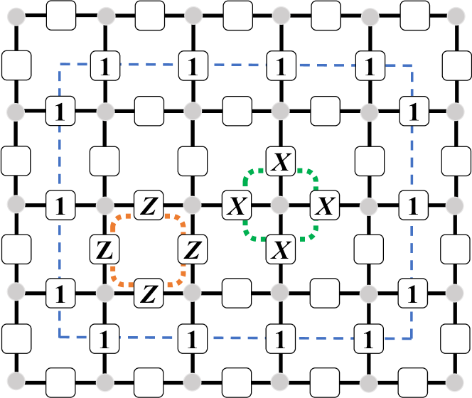
Figure 2: Toric code conventions: green dashed line represents the vertex operator $A_{v}$, the orange dashed line represents the plaquette operator $B_{p}$, and the blue dashed line gives an example of the quantum state related to closed-loop $l$.

We now calculate the overlap function $\Omega_{w,\mu}$ for the toric code state. Utilizing Eq. (5), we can demonstrate that the overlap function is given by:

$$\Omega_{w,\mu}=\frac{\prod_{i}N_{i}}{|\mathcal{C}|}\sum_{l\in\mathcal{C}}W_{l}.$$ (11)

Each loop configuration takes a weight of $W_{l}=\prod_{i\in l}W_{i}$ that can be effectively treated as the Boltzmann weight for a domain wall configuration in the Ising model. The overlap function is thus

$$\Omega_{w,\mu}\propto\sum_{s}\exp\left(\sum_{i=\langle k,l\rangle}K_{i}s_{k}s_{l}\right),$$ (12)

where

$$\exp(-2K_{i})=W_{i},$$ (13)

with $i=\langle k,l\rangle$ being the edge connecting site neighboring site $k$ and $l$ and the classical spins $\{s\}$ are defined on the vertices of the square lattice given in Fig. 2.

II.2 The Bipartite Cluster State

We now consider cluster states defined on bipartite graphs. The cluster state is a stabilizer state defined on a graph $G=(V,E)$, where the stabilizer generator takes the form

$$g_{i}=X_{i}\prod_{j\in\mathcal{N}_{i}}Z_{j}\quad i\in V.$$ (14)

where $j\in\mathcal{N}_{i}$ is the neighbor of vertex $i$, and the cluster state $\ket{\Psi}$ satisfies the stabilizer condition $g_{i}\ket{\Psi}=\ket{\Psi}$, for all sites $i$. For a bipartite graph $G$, the stabilizer generators naturally split into two sets:

$$g_{i} =X_{i}\prod_{j\in\mathcal{N}_{i}}Z_{j}\quad\text{for }i\in\circ$$ (15)

$$g_{m} =X_{m}\prod_{n\in\mathcal{N}_{m}}Z_{n}\quad\text{for }m\in\bullet,$$

where $\mathcal{N}_{i/m}$ denotes the neighbors of site $i/m$, and $\circ,\bullet\subset V$ labels the bipartition of graph vertices. Two examples of graph bipartition are shown in Fig. 3.

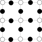
(a) Lieb lattice

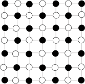
(b) Square lattice

Figure 3: Lattice bipartitions

Applying Hardmard rotation $\operatorname{H}$ on the $\bullet\in V$ sites of the bipartite cluster state, we have the hardmard rotated state $\ket{\Psi}_{H}=\prod_{i\in\bullet}\operatorname{H}_{i}\ket{\Psi}$, which is stabilized under

$$g_{i}^{X} =X_{i}\prod_{j\in\mathcal{N}_{i}}X_{j}\quad\text{for }i\in\circ$$ (16)

$$g_{m}^{Z} =Z_{m}\prod_{n\in\mathcal{N}_{m}}Z_{n}\quad\text{for }m\in\bullet,$$

as presented in [27]. The rotated quantum state $\ket{\Psi}_{H}$ can then be expressed as

$$\ket{\Psi}_{H} =\frac{1}{2^{N}}\prod_{m\in\bullet}(1+g_{m}^{Z})\prod_{i\in\circ}(1+g_{i}^{X})\bigotimes_{k\in\Lambda}\ket{0}_{k}$$ (17)

$$=\frac{1}{2^{|\circ|}}\prod_{i\in\circ}(1+g_{i}^{X})\bigotimes_{k\in\Lambda}\ket{0}_{k}$$

$$=\frac{1}{2^{|\circ|}}\sum_{A}g^{X}_{A}\bigotimes_{k\in\Lambda}\ket{0}_{k}.$$

Here, the rotated cluster state $\ket{\Psi}_{H}$ is given by applying projection operators $1/2(1+g_{m}^{Z})$ and $1/2(1+g_{i}^{X})$ to an initial state $\bigotimes_{k\in\Lambda}\ket{0}_{k}$. Taking advantage of the fact that $X\ket{0}=\ket{1}$ and $Z\ket{0}=\ket{0}$, we write the rotated cluster state in the following form

$$\ket{\Psi}_{H}=\frac{1}{2^{|\circ|}}\sum_{A}\ket{A}\otimes\ket{\partial A}\otimes\ket{\overline{A}}.$$ (18)

We use $A$ to denote $\circ$ sites that support $g_{A}^{X}$ and $\partial A$ to denote neighboring sites of $A$, which, because the lattice is bipartite, are $\bullet$, and $\overline{A}$ to denote other parts of the qubits. The quantum states $\ket{A}=\bigotimes_{A}\ket{1}$ and $\ket{\overline{A}}=\bigotimes_{\overline{A}}\ket{0}$. As for $\ket{\partial A}$, we take

$$\ket{\partial A}=\bigotimes_{i\in\mathcal{N}_{E},j\in\mathcal{N}_{O}}\ket{0}_{i}\ket{1}_{j}$$ (19)

where $\mathcal{N}_{E/O}$ denotes $\bullet$ sites that have even/odd number of $g_{i}^{X}$’s operating on the its $\circ$ neighbours. The overlap function is

$$\Omega_{w,\mu}\propto\sum_{A}W_{A}\times W_{\partial A}$$ (20)

where

$$W_{A} =\innerproduct{\mu_{A},w_{A}}{A}=\prod_{i\in A}W_{i}$$

$$W_{\partial A} =\innerproduct{\mu_{\partial A},w_{\partial A}}{\partial A}=\prod_{i\in\mathcal{N}_{O}}W_{i}$$

with $\ket{\mu_{A},w_{A}}$ and $\ket{\mu_{\partial A},w_{\partial A}}$ being the measurement basis on $A$ and $\partial A$

$$\ket{\mu_{A},w_{A}} =\bigotimes_{j\in A}\ket{\mu_{j},w_{j}}_{j}$$ (21)

$$\ket{\mu_{\partial A},w_{\partial A}} =\bigotimes_{i\in\partial A}\ket{\mu_{i},w_{i}}_{i}.$$

When introducing the Ising degrees of freedom $\{s\}$ on $\circ$ sites, $W_{A}$ can be treated as the onsite magnetic field term whereas the boundary $W_{\partial A}$ contributes to the spin interaction. Thus, the overlap function can be expressed in the form of an Ising partition function,

$$\innerproduct{\mu,w}{\Psi}_{H}\propto$$ (22)

$$\sum_{s} \exp\left(\sum_{i\in\bullet}K_{i}\prod_{j\in\mathcal{N}_{i}|j\in\circ}s_{j}+\sum_{k\in\circ}h_{k}s_{k}\right).$$

where the classical spins $\{s_{i}\}$ are defined on the $\circ$ sublattice. The effective multi-spin coupling constant $K_{i}$ is given by $\exp(-2K_{i})=W_{i}$ with $i\in\bullet$, and the onsite effective magnetic field is obtained from $\exp(-2h_{k})=W_{k}$ with $k\in\circ$. The overlap function of $\ket{\Psi}$ without Hardmard rotation can be obtained using the identity

$$\innerproduct{\mu,w}{\Psi}=\bra{\mu,w}\prod_{i\in\bullet}H_{i}^{\dagger}H_{i}\ket{\Psi}=\bra{\mu,w^{\prime}}\ket{\Psi}_{H}$$ (23)

where $W^{\prime}_{i}=W_{i}$ for $i\in\circ$, and $W^{\prime}_{i}=(1-W_{i})/(1+W_{i})$ for $i\in\bullet$ due to the Hardmard rotation on site $i\in\bullet$. The correspondence between the measurement parameter $\{W_{i},W_{k}\}$ and the Ising parameters $\{K_{i},h_{k}\}$ are now

$$\begin{matrix}&\exp(-2h_{k})=W_{k}&\quad k\in\circ\\ &\exp(-2K_{i})=\frac{1-W_{i}}{1+W_{i}}&\quad i\in\bullet\end{matrix}.$$ (24)

It should be noted that the variable $W_{i}$ is generally complex, implying that both $K_{j}$ and $h_{j}$ can take complex values. In Appendix A, an alternative approach for establishing a connection between the cluster state overlap function $\Omega_{w,\mu}$ and the Ising partition function $\mathcal{Z}$ is presented.

One simple example is the cluster state defined on the Lieb lattice, the bipartition of such lattice is shown in Fig. 3a, where the vertices are labeled “$\circ$” while the edges are “$\bullet$”, and an example of $\ket{A}\otimes\ket{\partial A}\otimes\ket{\overline{A}}$ is shown in Fig. 4. Following the same logic, we write down the overlap function as

$$\Omega_{w,\mu}\propto\sum_{s}\exp\left(\sum_{m=\langle i,j\rangle}K_{m}s_{i}s_{j}+\sum_{k}h_{k}s_{k}\right).$$ (25)

This is the partition function of the Ising model with nearest neighbor coupling in the presence of the magnetic field. The classical Ising spin is defined on the $\circ$ sublattice, which forms a square lattice. The parameters $K_{m}$ and $h_{k}$ are given by Eq. 24.

An interesting scenario is when taking the measurement on the vertex direction to be $X$ and forcing the measurement outcome to be $\mu_{i}=+$, which means that for vertex sites $w_{i}=1$ and thus $h_{i}=0$. The wave function with forced $X$ measurements on the vertices takes the form

$$\ket{\Psi}^{+}=\left(\sum_{\mu_{\bullet}}\Omega_{w,\mu,h=0}\ket{\mu,w}_{\bullet}\right)\otimes\ket{+}_{\circ}$$ (26)

where $\{\ket{\mu,w}_{\bullet}\}$ is the edge measurement basis, and $\ket{+}_{\circ}\equiv\bigotimes_{i\in\circ}\ket{+}_{i}$ is the tensor product of $+$ eigenstates of Pauli $X$ on the vertices. As $\Omega_{w,\mu,h=0}$ is the same as the overlap function of the toric code shown in Eq. 12 up to Hardmard rotations, we thus have

$$\ket{\Psi}^{+}=\ket{\Psi}^{TC}_{H}\otimes\ket{+}_{\circ}$$ (27)

with

$$\ket{\Psi}^{TC}_{H}=\frac{1}{|\mathcal{C}|}\sum_{l\in\mathcal{C}}\ket{l}_{H}~{}\text{and}~{}\ket{l}=\bigotimes_{i\in l,j\not\in l}\ket{+}_{i}\otimes\ket{-}_{j}$$ (28)

where $X_{i}\ket{\pm}_{i}=\pm\ket{\pm}_{i}$. One subtlety here is that the quantum state obtained via vertex $X$ measurement differs from the toric code state shown in Eq. 9 by Hardmard rotations on each unmeasured sits, and the loops are represented in $\ket{\pm}$ instead of $\ket{0},\ket{1}$.

The $X$ measurements on the vertices can also be interpreted as enforcing flux constraints in $\mathbb{Z}_{2}$ gauge theory:

$$\mathcal{Z}=\sum_{\tau}\exp\left(\sum_{p=\langle a,b\rangle^{\prime}}\tilde{h_{p}}\tau_{p}\right)\prod_{i}(1+m_{i}\prod_{q\in\square_{i}}\tau_{q}).$$ (29)

Here, $\tau_{p}$ represents the $\mathbb{Z}_{2}$ gauge field defined on edge $p$, $a,b$ are neighboring plaquettes that share the same edge $p$, and $\prod_{i}(1+m_{i}\prod_{q\in\square_{i}}\tau_{q})$ denotes the flux constraint associated with the $X$ measurement outcome $m_{i}=\pm 1$ on vertex $i$, with $\prod_{q\in\square_{i}}$ being the product over edges sharing the same vertex $i$. By enforcing $m_{i}=1$ for all vertices $i$, we recover the Ising partition function by directly setting $\tau_{q}=\sigma_{a}\sigma_{b}$, where $\sigma_{a}\sigma_{b}$ are $\mathbb{Z}_{2}$ variables assigned to plaquettes $a$ and $b$. A detailed discussion can be found in Appendix C.

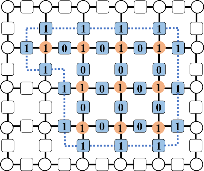
Figure 4: Example structure of wave function $\ket{A}\otimes\ket{\partial A}\otimes\ket{\overline{A}}$. The orange dots are $\ket{A}$, $\ket{\partial A}$ is colored in Blue, and the un-colored part labels $\ket{\overline{A}}$. The blue dashed line labels the $\prod_{j\in\mathcal{N}_{O}}\ket{1}_{j}$ part of $\ket{\partial A}$

Another example is the cluster state defined square lattice state in our previous work [24]. With the bipartition shown in Fig. 3b, the overlap function for this case is

$$\Omega_{w,\mu}\propto\sum_{s}\exp(\sum_{i\in\bullet}K_{i}s_{a}s_{b}s_{c}s_{d}+\sum_{r\in\circ}h_{r}s_{r})$$ (30)

where the Ising spins $\{s\}$ locate on $\circ$ sites. The four-body Ising interaction $K_{i}s_{a}s_{b}s_{c}s_{d}$ is defined on four neighboring sites $a,b,c,d\in\circ$ enclosing site $i\in\bullet$. The effective Ising coupling $\{K_{i}\}$ and magnetic field $\{h_{r}\}$ are determined by Eq. 24.

In summary, we show that the overlap function for the ground state of the toric code model and cluster state defined on the bipartite graph can be expressed in terms of classical Ising partition function $\Omega_{w,\mu}=\mathcal{Z}(K,h)$, as shown in Eq. 12, Eq. 25, and Eq. 30. The quantum sampling over such resouce states are therefore equivalent to the computation of the corresponding Ising partition function with complex parameters. In the subsequent sections of this paper, we will establish the connection between the hardness of approximating this partition function and the entanglement scaling of the 1D boundary state. We will show that by varying the measurement direction $\{w\}$, the boundary state can undergo a volume-law to an area-law entanglement phase transition. This transition, in turn, suggests that the resource state sampling problem can transition from being hard-to-simulate to becoming easy-to-simulate, depending on the measurement direction.

III Boundary States and Ising Partition Functions

In this section, we explore the boundary state that arises from measuring the bulk qubits in the previously discussed 2D quantum states. Specifically, we examine the 2D quantum state supported on a half-cylinder denoted as $\mathcal{M}$, as illustrated in Fig. 5. By using Eq.(6), we have

$$\ket{\Psi}_{\partial\mathcal{M}}\propto\sum_{\mu_{\partial\mathcal{M}}}\sum_{s}\exp{(H[s])}\ket{\mu_{\partial\mathcal{M}},w_{\partial\mathcal{M}}},$$ (31)

where the summation $\sum_{\mu_{\partial\mathcal{M}}}\sum_{s}$ is over all the spin configurations and boundary basis, and

$$\sum_{s}\exp{(H[s])}\propto\innerproduct{\mu_{\mathcal{M}},w_{\mathcal{M}},\mu_{\partial\mathcal{M}},w_{\partial\mathcal{M}}}{\Psi}$$ (32)

where $\ket{\mu_{\mathcal{M}},w_{\mathcal{M}},\mu_{\partial\mathcal{M}},w_{\partial\mathcal{M}}}\equiv\ket{\mu_{\mathcal{M}},w_{\mathcal{M}}}\otimes\ket{\mu_{\partial\mathcal{M}},w_{\partial M}}$ is the tensor product of the bulk measurement basis $\{\ket{\mu_{\mathcal{M}},w_{\mathcal{M}}}\}$ and the boundary basis $\{\ket{\mu_{\partial\mathcal{M}},w_{\partial\mathcal{M}}}\}$. We will further show that by properly choosing the boundary basis $\{\ket{\mu_{\partial\mathcal{M}},w_{\partial\mathcal{M}}}\}$, the boundary state can be written in a more compact form as

$$\ket{\Psi}_{\partial\mathcal{M}}\propto\sum_{s}\exp{(H[s])}\ket{s_{\partial\mathcal{M}}},$$ (33)

where $\{\ket{s_{\partial\mathcal{M}}}\}$ is a set of complete basis of the boundary labeled by classical boundary spin configuration $\{s_{\partial\mathcal{M}}\}$.

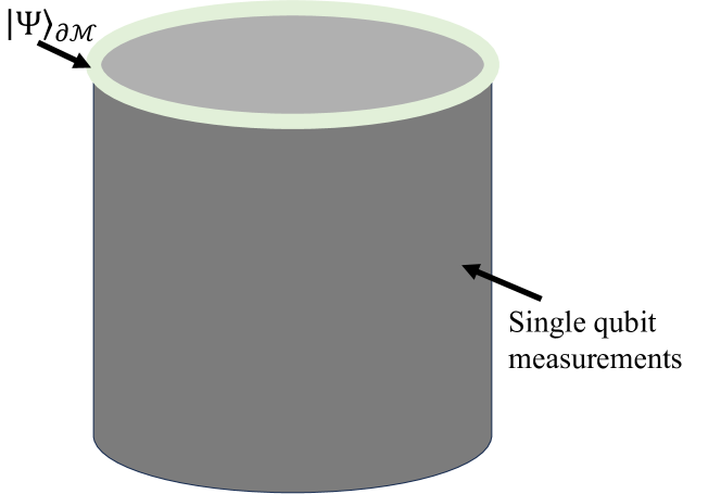
Figure 5: The 2D quantum state is defined on the half-cylinder $\mathcal{M}$. We perform single-qubit measurement in the bulk and leave the boundary $\partial\mathcal{M}$ (top circle) qubits unmeasured. $\ket{\Psi}_{\partial\mathcal{M}}$ denotes the 1D wave function on the unmeasured boundary.

We first consider the toric code model with a smooth boundary as shown in Fig. 6. We now express the boundary state in Pauli-$Z$ basis $\ket{\mu_{\partial\mathcal{M}}}\equiv\bigotimes_{i\in\partial\mathcal{M}}\ket{\mu_{i}}_{i}$, with $\mu_{\partial\mathcal{M}}\equiv(\mu_{1},\mu_{2},\ldots,\mu_{L})$, and $Z_{i}\ket{\mu_{i}}_{i}=\mu_{i}\ket{\mu_{i}}_{i}$. The boundary basis is effectively taking $\theta_{i}\to 0$ in Eq. 3 on the boundary, and the local weight parameter $W_{i}$ defined in Eq 4 is then

$$W_{i}=\lim_{\theta\to 0}\left\{\begin{matrix}\tan(\theta_{i}/2)\exp(i\varphi_{i})&\text{if}&\mu=+1\\ \cot(\theta_{i}/2)\exp(-i\varphi_{i})&\text{if}&\mu=-1\end{matrix}\right..$$ (34)

For simplicity, we choose the limit direction to be $0^{+}$ to fix the sign of the weight parameter when the measurement outcome is negative $\mu=-1$

$$W_{i}=\lim_{\theta\to 0^{+}}\left\{\begin{matrix}0&\text{if}&\mu=+1\\ +\infty&\text{if}&\mu=-1\end{matrix}\right.$$ (35)

and we thus have the boundary coupling

$$K_{i}=\left\{\begin{matrix}+\infty&\text{if}&\mu=+1\\ -\infty&\text{if}&\mu=-1\end{matrix}\right..$$ (36)

This can be further written as

$$\tanh K_{i}=\mu_{i}\quad i\in\partial\mathcal{M}$$ (37)

Figure 6: Toric code with smooth boundary conditions. Green shaded area denotes the unmeasured boundary qubits. The vertex stabilizer $A_{v}=\prod_{i}X_{i}$ and plaquette stabilizer $B_{p}=\prod_{i}Z_{i}$ living on the boundary are labeled by orange dashed lines.

The boundary state of the toric code can be expressed as follows:

$$\ket{\Psi}_{\partial\mathcal{M}}\propto \sum_{s,\mu_{\partial\mathcal{M}}}\exp\left(\sum_{j=\langle c,d\rangle}K_{j}s_{c}s_{d}\right)\times$$ (38)

$$\exp\left(\sum_{i=\langle a,b\rangle}K_{i}s_{a}s_{b}\right)\ket{\mu_{\partial\mathcal{M}}}.$$

Here, the first sum, denoted by $\sum_{j=\langle c,d\rangle}$, represents the summation over the links of the bulk of the square lattice, while the second summation $\sum_{i=\langle a,b\rangle}$ is the sum over the links that lie on the boundary. Taking advantage of Eq. 37, we further write the boundary summation as

$$\exp\left(\sum_{i=\langle a,b\rangle}K_{i}s_{a}s_{b}\right)\propto\prod_{i=\langle a,b\rangle}(1+\tanh K_{i}s_{a}s_{b})$$ (39)

$$=\prod_{i=\langle a,b\rangle}(1+\mu_{i}s_{a}s_{b})\propto\prod_{i\in\partial\mathcal{M}}\delta_{\mu_{i},s_{a}s_{b}}$$

where we used the fact that $\prod_{i=\langle a,b\rangle}(1+\mu_{i}s_{a}s_{b})\neq 0$ if and only if $\mu_{i}=s_{a}s_{b}$ for all $i$. The boundary state for toric code can now be written as

$$\ket{\Psi}_{\partial\mathcal{M}} \propto\sum_{\mu_{\partial\mathcal{M}}}\sum_{s}\exp\left(\sum_{j=\langle c,d\rangle}K_{j}s_{c}s_{d}\right)\prod_{i\in\partial\mathcal{M}}\delta_{\mu_{i},s_{a}s_{b}}\ket{\mu_{\partial\mathcal{M}}}$$ (40)

$$\propto\sum_{s}\exp\left(\sum_{j=\langle c,d\rangle}K_{j}s_{c}s_{d}\right)\bigotimes_{i=\langle a,b\rangle}\ket{s_{a}s_{b}}_{i}.$$

where $\ket{s_{a}s_{b}}_{i}$ represents the quantum state on the $i$-th qubit of the boundary, satisfying $Z_{i}\ket{s_{a}s_{b}}_{i}=s_{a}s_{b}\ket{s_{a}s_{b}}_{i}$, with $i$ being the edge connecting neighboring sites $a$ and $b$. This quantum state is determined by the corresponding classical Ising domain wall configuration on the boundary, denoted as $\{s_{a}s_{b}\}$ with $a,b$ being neighbors. With this, we complete the construction of the boundary state for the toric code model.

For the boundary state of the Lieb cluster, similar to the toric code case, we take the basis

$$\ket{\mu_{\partial\mathcal{M}}}\equiv\big{(}\bigotimes_{i\in\partial\mathcal{M}_{\bullet}}\ket{\mu_{i}}_{i}\big{)}\otimes\big{(}\bigotimes_{a\in\partial\mathcal{M}_{\circ}}\ket{\mu_{a}}_{a}\big{)}.$$ (41)

For the boundary edge qubit $i\in\partial\mathcal{M}_{\bullet}$, we define the basis as follows

$$X_{i}\ket{\mu_{i}}_{i}=\mu_{i}\ket{\mu_{i}}_{i}.$$ (42)

For the boundary vertex qubit $a\in\partial\mathcal{M}_{\circ}$, the basis is

$$Z_{a}\ket{\mu_{a}}_{a}=\mu_{a}\ket{\mu_{a}}_{a}.$$ (43)

To obtain these basis via the measurement basis defined in Eq. 1, we take $\theta_{i}\to\pi/2$ and $\phi_{i}\to 0$ in the Eq. 3. On the other hand, the basis for the vertex qubit $a\in\partial\mathcal{M}_{\circ}$ is acquired by performing a Pauli $Z$ measurement with $\theta_{i}\to 0$.

For the edge qubit, the corresponding weight parameter, defined in Eq. 4, of such basis is then

$$W_{i}=\left\{\begin{matrix}1&\text{if}&\mu_{i}=+1\\ -1&\text{if}&\mu_{i}=-1\end{matrix}\right..$$ (44)

As $\exp(-2K_{i})=(1-W_{i})/(1+W_{i})$, the corresponding boundary coupling is

$$K_{i}=\left\{\begin{matrix}+\infty&\text{if}&\mu_{i}=+1\\ -\infty&\text{if}&\mu_{i}=-1\end{matrix}\right..$$ (45)

Again we write

$$\tanh K_{i}=\mu_{i}\quad i\in\partial\mathcal{M}_{\bullet}$$ (46)

As for the boundary vertex qubit, we have

$$W_{a}=\left\{\begin{matrix}0&\text{if}&\mu_{a}=+1\\ +\infty&\text{if}&\mu_{a}=-1\end{matrix}\right..$$ (47)

The corresponding magnetic field is then

$$h_{a}=\left\{\begin{matrix}+\infty&\text{if}&\mu_{a}=+1\\ -\infty&\text{if}&\mu_{a}=-1\end{matrix}\right.,$$ (48)

which can be further written as

$$\tanh h_{a}=\mu_{a}\quad a\in\partial\mathcal{M}_{\circ}.$$ (49)

We now write the boundary state of the Lieb cluster state as

$$\ket{\Psi}_{\partial\mathcal{M}} \propto\sum_{\mu_{\partial\mathcal{M}}}\sum_{s}\exp{\sum_{j=\langle c,d\rangle}K_{j}s_{c}s_{d}+\sum_{e}h_{e}s_{e}}$$ (50)

$$\times \exp{\sum_{i=\langle a,b\rangle}K_{i}s_{a}s_{b}+\sum_{c}h_{c}s_{c}}\ket{\mu_{\partial\mathcal{M}}},$$

where the first line is the bulk term and the second term is the boundary term. The boundary terms can be further written as

$$\exp{\sum_{i=\langle a,b\rangle}K_{i}s_{a}s_{b}+\sum_{c}h_{c}s_{c}}$$ (51)

$$\propto\prod_{i=\langle a,b\rangle}(1+\tanh K_{i}s_{a}s_{b})\prod_{c}(1+\tanh h_{c}s_{c})$$

$$\propto\prod_{i=\langle a,b\rangle}\delta_{\mu_{i}s_{a}s_{b}}\prod_{c}\delta_{\mu_{c}s_{c}}.$$

where we used the same derivation in Eq. 39. We may thus relabel the boundary basis using the boundary Ising spin variables

$$\begin{matrix}\mu_{i}=s_{a}s_{b}&&i\in\partial\mathcal{M}_{\bullet}\\ \mu_{c}=s_{c}&&c\in\partial\mathcal{M}_{\circ}\end{matrix}$$ (52)

where $i=\langle a,b\rangle$ is the edge connecting neighboring sites $a,b$. The boundary state of the Lieb lattice model is thus

$$\ket{\Psi}_{\partial\mathcal{M}} \propto\sum_{s}\exp{\sum_{j=\langle c,d\rangle}K_{j}s_{c}s_{d}+\sum_{e}h_{e}s_{e}}\times$$ (53)

$$\bigotimes_{i=\langle a,b\rangle,c}\ket{s_{a}s_{b}}_{i}\ket{s_{c}}_{d}.$$

where the boundary basis satisfies

$$\begin{matrix}X_{i}\ket{s_{a}s_{b}}_{i}=s_{a}s_{b}\ket{s_{a}s_{b}}_{i}&i\in\partial\mathcal{M}_{\bullet}\\ Z_{c}\ket{s_{c}}_{c}=s_{c}\ket{s_{c}}_{c}&c\in\partial\mathcal{M}_{\circ}\end{matrix}.$$ (54)

It is thus obvious that the boundary state is the eigenstate of $g_{i}=X_{i}Z_{a}Z_{b}$ with $a,b$ being neighboring boundary sites connected by edge $i$

$$g_{i}\ket{\Psi}_{\partial\mathcal{M}}=\ket{\Psi}_{\partial\mathcal{M}}\quad\forall i\in\partial\mathcal{M}_{\bullet}.$$ (55)

The boundary state of the cluster state on the square lattice is obtained using a similar approach as the one defined on the Lieb lattice. The boundary state is

$$\ket{\Psi}_{\partial\mathcal{M}}\propto$$ (56)

$$\sum_{s} \exp{\sum_{j\in\bullet}K_{j}s_{e}s_{f}s_{g}s_{h}+\sum_{r\in\circ}h_{r}s_{r}}$$

$$\bigotimes_{i,d}\ket{s_{a}s_{b}s_{c}}_{i}\ket{s_{d}}_{d}$$

where $j$ is the bulk $\bullet$ site enclosed by neighboring $\circ$ sites $e,f,g,h$, and $i$ labels the boundary $\bullet$ sites enclosed by $a,b,c\in\circ$, as shown in Fig. 8b. The boundary basis satisfies

$$X_{i}\ket{s_{a}s_{b}s_{c}}_{i} =s_{a}s_{b}s_{c}\ket{s_{a}s_{b}s_{c}}_{i}$$ (57)

$$Z_{d}\ket{s_{d}}_{d} =s_{d}\ket{s_{d}}_{d}$$

We thus finish the derivation of the boundary state in terms classical Ising model.

(a) Lieb lattice with smooth boundary. Green shaded area: boundary qubits. $a,b\in\circ$ label the neighboring sites of $i\in\bullet$. $c$ labels the boundary $\circ$ sites.

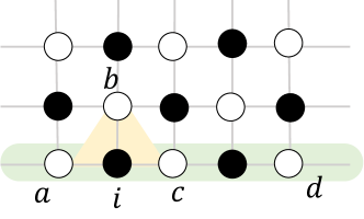
(b) The boundary of the square lattice cluster state. $a,b,c$ label the neighboring sites of $i\in\bullet$. $d$ labels the boundary $\circ$ sites.

Figure 7: Boundary conventions

To sum up, in this section, we have demonstrated that the boundary state, which is obtained through single qubit projective measurements on the bulk qubits, carries crucial information about the partition function of the 2D classical Ising model. Consequently, if we can successfully compute the 1D boundary state for a large system, we can effectively solve the 2D state sampling problem. One promising method for approximately simulating 1D quantum states is the MPS approach. The complexity of this representation relies on the entanglement scaling of the wave function. If the wave function exhibits volume-law scaling of entanglement, storing this quantum state becomes challenging, and consequently, computing the corresponding partition function becomes difficult. However, if the state follows an area-law scaling of entanglement, it can be efficiently approximated on a classical computer, making approximately compute the corresponding partition function relatively easy. In the next section, we will elaborate on the formalism to compute the boundary state by mapping it to a 1+1D dynamical problem. This approach will provide further insights into understanding and addressing the complexity of the quantum sampling problem.

IV Bridging 2D Sampling Problem and 1+1D Circuit Dynamics

In the previous section, we demonstrated that for a cluster state defined on a bipartite graph, the boundary 1D quantum state can be expressed as follows after performing single qubit measurements on the bulk qubits:

$$\ket{\Psi}_{\partial\mathcal{M}}\propto\sum_{s}\exp{(H[s])}\ket{s_{\partial\mathcal{M}}}$$ (58)

Here $H[s]$ represents a 2D classical spin Hamiltonian with parameters that can take complex values, and $\ket{s_{\partial\mathcal{M}}}$ is the basis for the boundary state related to the classical-spin configurations on the boundary. This boundary state exhibits entanglement transitions and establishes an interesting connection with the 1+1D hybrid quantum dynamics. In this section, we provide two approaches to dynamically generate this boundary state.

IV.1 Transfer Matrix Method

It is well-established that the partition function of the 2D classical spin model is connected to the 1+1D quantum dynamics using the transfer matrix method as in Fig. 9. Consequently, the boundary wave function in Eq. (58) can be expressed as follows:

$$\ket{\Psi}_{\partial\mathcal{M}}=\mathcal{T}\prod_{\tau}\mathbf{T}(\tau)\ket{\Psi_{0}}$$ (59)

where $\mathcal{T}$ is the time ordering operator, $\mathbf{T}(\tau)$ is the the transfer matrix acting on the initial state $\ket{\Psi_{0}}$. The initial state $\ket{\Psi_{0}}$ is determined by the shape of the bottom boundary as shown in Fig. 9.

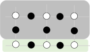
(a) The ”smooth” boundary

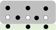
(b) The ”rough” boundary

Figure 8: Typical boundary shapes of Lieb lattice

For the cluster state defined on the Lieb lattice, two typical boundaries are the “smooth” and “rough” boundaries, as shown in Fig. 8. For ”smooth boundary,” $\ket{\Psi_{0}}$ is the equal weight superposition of quantum states labeled by all possible boundary classical spin configurations $\{s_{\partial\mathcal{M}}\}$

$$\ket{\Psi_{0}}=\frac{1}{2^{|\{s_{\partial\mathcal{M}}\}|}}\sum_{s_{\partial\mathcal{M}}}\ket{s_{\partial\mathcal{M}}},$$ (60)

while for “rough” boundary conditions, we have

$$\ket{\Psi_{0}}=\ket{s_{\partial_{M}}=+1}.$$ (61)

A detailed discussion of the boundary condition is shown in App. B. In the following, we will use the term “top boundary” to refer to qubits support the wave function induced by bulk measurement $\ket{\Psi}_{\partial\mathcal{M}}$, and “bottom boundary” to refer qubits on the other end of the cylinder $\mathcal{M}$ which determines the initial state $\ket{\Psi_{0}}$.

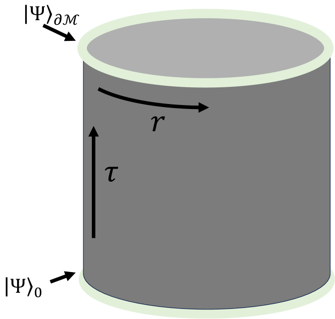
Figure 9: The two “dimensions” are now labeled as the spatial dimension $r$ and the temporal dimension $\tau$. $\ket{\Psi}_{\partial\mathcal{M}}$ is obtained by “time” evolution of initial state $\ket{\Psi}_{0}$.

The 1D boundary state $\ket{\Psi}_{\partial\mathcal{M}}$ is defined in Eq. 53. We take the perpendicular axis as the temporal direction $\hat{\tau}$ and the horizontal axis as the spatial direction $\hat{r}$ shown in Fig. 9. We will use “time slice $\tau$” to refer to the row position of a vertex site. The indices $a,b,c,\ldots$ denote the column position, and $i,j,k,\ldots$ are used to label the edges connecting neighboring vertex sites. We will use $i=\langle a,b\rangle$ to label the edge $i$ connecting neighboring sites $a$ and $b$, and $e=(k,l)$ to label vertex $e$ shared by neighboring edges $k$ and $l$.

For the Ising model defined on the square lattice, it is well-known that by associating each vertex with a qubit, we obtain the spin basis for each time slice $\tau$

$$\ket{s}_{\tau}=\bigotimes_{a\in\tau}\ket{s_{a}}_{a}\quad Z_{a}\ket{s_{a}}_{a}=s_{a}\ket{s_{a}}_{a},$$ (62)

which spans the Hilbert space $\mathcal{H}_{\tau}=\operatorname{span}\{\ket{s}_{\tau}\}$. The transfer matrix that maps $\mathcal{H}_{\tau}$ to $\mathcal{H}_{\tau+1}$ can now be written in the form

$$T(\tau)=T_{2}(\tau)T_{1}(\tau)$$ (63)

with

$$T_{1}(\tau)\propto\exp\left(\sum_{\begin{subarray}{c}i=\langle a,b\rangle\end{subarray}}K^{\tau}_{i}Z_{a}^{\tau}Z_{b}^{\tau}+\sum_{c}h^{\tau}_{c}Z_{c}^{\tau}\right)$$ (64)

$$T_{2}(\tau)\propto\exp(\sum_{e}\tilde{K}_{e}^{\tau}X_{e}^{\tau})$$

with $K_{i}^{\tau}$ being the quantum Ising coupling, $\tilde{K}_{e}^{\tau}$ the effective transverse field, and $h_{c}^{\tau}$ the longitudinal field. The Paulis are defined in the following way

$$Z_{a}^{\tau} \equiv\sum_{s_{a_{\tau}}}\ket{s_{a_{\tau}}}_{a_{\tau}}\bra{s_{a_{\tau}}}_{a_{\tau}}$$ (65)

$$X_{e}^{\tau} \equiv\sum_{s_{e_{\tau}}}\ket{\overline{s_{e_{\tau}}}}_{e_{\tau+1}}\bra{s_{e_{\tau}}}_{s_{e_{\tau}}}$$

where $\overline{s_{e_{\tau}}}\equiv-s_{e_{\tau}}$. As $\mathcal{H}_{\tau}$’s are identical for all time slice $\tau$, we will drop the index $\tau$ on the Pauli’s as well as on the classical spin indices labeling the quantum states in the remaining part of this section. The relations between the quantum parameters $\{K^{\tau},\tilde{K}^{\tau},h\}$ and the classical parameters $\{K,h\}$ are shown below

$$K_{i}^{\tau} =K_{i_{\tau}}$$ (66)

$$h_{c}^{\tau} =h_{c_{\tau}}$$

$$\tilde{K}_{e}^{\tau} =-\frac{1}{2}\ln\tanh{K_{e_{\tau}}}$$

where $K_{i_{\tau}}$ is the classical coupling along the spatial direction $\hat{r}$ on the $i$-th edge of time slice $\tau$, $h_{c_{\tau}}$ is the classical magnetic field on site $c$ at time slice $\tau$, and $K_{e_{\tau}}$ is the classical coupling along the temporal direction $\hat{\tau}$ of neighboring sites on time slice $\tau$ and $\tau+1$ of the $e$-th row of vertex sites.

In the Lieb lattice model, the qubits are on both the vertices and edges of the square lattice. Notice that the $1$d quantum state on the boundary $\ket{\Psi}_{\partial\mathcal{M}}$ is defined on the Pauli-$X$ basis for $\circ$ vertices and the Pauli-$Z$ basis for $\bullet$ edges as shown in the previous section. The basis for the transfer matrix of the Lieb lattice model is naturally

$$\ket{s}_{\text{Lieb}}=\bigotimes_{i,c}\ket{s_{a}s_{b}}_{i}\otimes\ket{s_{c}}_{c}$$ (67)

as defined in Eq.54, with $i\in\bullet$ labeling the boundary edge connecting vertex $a,b$, and $c\in\circ$ the boundary vertex. On such basis, the transverse field part is modified to

$$\mathbf{T}_{2}(\tau)\propto\exp(\sum_{e=(k,l)}\tilde{K}_{e}^{\tau}X_{e}Z_{k}Z_{l}),$$ (68)

where again $\tilde{K}_{e}^{\tau}=-1/2\ln\tanh K_{e_{\tau}}$ with $K_{e_{\tau}}$ being the classical coupling along $\hat{\tau}$ that connects neighboring sites of $e$-th row of vertices on time slice $\tau$ and $\tau+1$. Here, $X_{e}$ is a Pauli $X$ operator on the vertex qubit $e$, and $Z_{k}$, $Z_{l}$ are $Z$ Paulis operators on neighboring edges in the spacial direction $k,l\in\hat{r}$ that share the same vertex $e$. Since the edge qubits

$$Z_{k}\ket{s_{e}s_{g}}_{k}=\ket{\overline{s_{e}s_{g}}}_{k},$$ (69)

where $\ket{s_{e}s_{g}}_{k}$ and $\ket{\overline{s_{e}s_{g}}}_{k}$ are the eigenstates of $X_{k}$, operator $X_{e}Z_{k}Z_{l}$ flips the classical spin defined on vertex $e$ in the following manner

$$X_{e}Z_{k}Z_{l} \ket{s_{e}}_{e}\ket{s_{e}s_{g}}_{k}\ket{s_{e}s_{h}}_{l}$$ (70)

$$=\ket{\overline{s_{e}}}_{e}\ket{\overline{s_{e}s_{g}}}_{k}\ket{\overline{s_{e}s_{f}}}_{l}$$

$$=\ket{\overline{s_{e}}}_{e}\ket{\overline{s_{e}}s_{g}}_{k}\ket{\overline{s_{e}}s_{f}}_{l}.$$

Here $e=(k,l)$ is the site shared by two edges $k$ and $l$.

The spatial coupling of the Lieb lattice model $\mathbf{T}_{1}(\tau)$ is the same as $T_{1}(\tau)$ for the Ising model defined on a square lattice, since Pauli $Z$ transforms spin-edge basis Eq. 67 the same way as the spin basis Eq. 62. The transfer matrix $\mathbf{T}(\tau)=\mathbf{T}_{1}(\tau)\mathbf{T}_{2}(\tau)$ at time $\tau$ is thus obtained.

The initial state $\ket{\Psi}_{0}$ for both “smooth” and “rough” boundaries can be expanded using the basis defined in Eq. 67

$$\ket{s}_{\text{Lieb}}=\bigotimes_{i,c}\ket{s_{a}s_{b}}_{i}\otimes\ket{s_{c}}_{c},$$

which is stabilized under $g_{i}=X_{i}Z_{a}Z_{b}$ for all edge $i=\langle a,b\rangle$. Since

$$[g_{i},\mathbf{T}(\tau)]=0\quad\forall i,\tau$$ (71)

the boundary state state $\ket{\Psi}_{\partial\mathcal{M}}$ obtained by evolving $\ket{\Psi}_{0}$ is still an eigenstate of $g_{i}$. This is consistent with Eq. 55. We thus finish the derivation of the transfer matrix of the cluster state defined on the Lieb lattice.

IV.2 Connection with 1+1D Circuit Dynamics

The transfer matrix of the Lieb lattice model obtained in Sec. IV.1 can be decomposed into three types of local gates in the following way

$$\mathbf{T}(\tau)\propto \exp\left(\sum_{\begin{subarray}{c}i=\langle a,b\rangle\end{subarray}}K^{\tau}_{i}Z_{a}Z_{b}+\sum_{c}h^{\tau}_{c}Z_{c}\right)$$ (72)

$$\times\exp(\sum_{e=(k,l)}\tilde{K}_{e}^{\tau}X_{e}Z_{k}Z_{l})$$

$$= \prod_{i}\mathbf{T}_{ZZ}^{i=\langle a,b\rangle}(\tau)\prod_{c}\mathbf{T}_{Z}^{c}(\tau)\prod_{e}\mathbf{T}_{X}^{e=(k,l)}(\tau),$$

where

$$\mathbf{T}_{ZZ}^{i=\langle a,b\rangle}(\tau)=\exp(K_{i}^{\tau}Z_{a}Z_{b})$$ (73)

is a two-qubit gate and characterizes the Ising interaction between neighboring qubits $a$ and $b$,

$$\mathbf{T}_{Z}^{c}(\tau)=\exp(h_{c}Z_{c}),$$ (74)

is a single qubit gate and represents the longitudinal field acting on vertex qubit $c$, and

$$\mathbf{T}_{X}^{e=(k,l)}(\tau)=\exp(\tilde{K}_{e}^{\tau}X_{e}Z_{k}Z_{l})$$ (75)

is a three-qubit gate, where $e=(k,l)$ is the vertex connecting two neighboring edges $k$ and $l$.

Taking advantage of Eq.24 and Eq.66, the correspondence between parameters in the quantum gates $\{K^{\tau},\tilde{K}^{\tau},h^{\tau}\}$ and the weight parameters $\{W\}$ defined in Eq. 4 is then

$$\begin{aligned} \exp(-2K_{i}^{\tau})&=\frac{1-W_{i_{\tau}}}{1+W_{i_{\tau}}}\\ \exp(-2\tilde{K}_{e}^{\tau})&=W_{e_{\tau}}\\ \exp(-2h_{c}^{\tau})&=W_{c_{\tau}}\\ \end{aligned},$$ (76)

where $W_{i_{\tau}}$ and $W_{e_{\tau}}$ are weight parameters on edges in spatial $\hat{r}$ and temporal $\hat{\tau}$ direction respectively. Here $i_{\tau}$ is the $i$-th edge on time slice $\tau$ and $e_{\tau}$ labels the edge connecting neighboring sites on the $e$-th row of vertex sites on time slice $\tau$ and $\tau+1$. $W_{c_{\tau}}$ is the measurement weight parameter on vertex site $c$ of time slice $\tau$. For measurements in the $XZ$-plane, the weight parameter $W\in\mathbb{R}$. For measurements containing $Y$ components, the weight parameter $W$ becomes complex, and the parameters in both the classical 2D Hamiltonian and 1+1D quantum dynamics are complex.

IV.2.1 Pauli Measurements

To illustrate the correspondence between the $2$d measurement process and the $1+1$d circuit dynamics and to understand the physical meaning of the complex Ising parameters, we examine three straightforward cases: measuring all the bulk qubits along the $X$, $Z$, and $Y$ directions. We show that bulk measurements along $X$ and $Z$ directions can be effectively treated as projective measurements in the $1+1$d circuit dynamics, while bulk $Y$ measurements are effective unitary gates.

When measuring the bulk along $X$ direction, we take $W=\pm 1$, where the $\pm$ sign is determined by measurement outcome. For every site in bulk, we have

$$\begin{aligned} K_{i}^{\tau}&=\pm\infty\\ \tilde{K}_{e}^{\tau}&=0\text{ or }\pm\frac{i\pi}{2}\\ h_{c}^{\tau}&=0\text{ or }\pm\frac{i\pi}{2}\\ \end{aligned}.$$ (77)

The local terms are

$$\begin{aligned} \mathbf{T}_{ZZ}^{i=\langle a,b\rangle}(\tau)&\propto(1\pm Z_{a}Z_{b})\\ \mathbf{T}_{Z}^{c}(\tau)&\propto I\text{ or }Z_{c}\\ \mathbf{T}_{X}^{e=(k,l)}(\tau)&\propto I\text{ or }X_{e}Z_{k}Z_{l}\\ \end{aligned}.$$ (78)

In this case, $\mathbf{T}_{ZZ}^{i=\langle a,b\rangle}(\tau)$ is effectively a $Z_{a}Z_{b}$ projective measurement on neighboring sites $a$ and $b$ connected by edge $i$, and $\mathbf{T}_{Z}^{c}(\tau)$ and $\mathbf{T}_{X}^{e=(k,l)}(\tau)$ are local Pauli operations that do not affect the entanglement structure.

The boundary state $\ket{\Psi}_{\partial\mathcal{M}}$ is a trivial product state stabilized under $\langle X_{i},Z_{a}\rangle$ with $i$ being the boundary edges and $a$ the vertices, if taking the “rough” boundary on the bottom and is a GHZ state on vertices and product state on edges stabilized under $\langle X_{i},Z_{a}Z_{b},\prod_{j}X_{j}\rangle$ with $i=\langle a,b\rangle$ being the edges, and $\prod_{j}X_{j}$ the $X$-string support on all the boundary edge qubits if taking the “smooth” boundary condition. This difference is because “smooth” bottom boundary condition preserves the global $\mathbb{Z}_{2}$ of Ising when measuring every site along $X$, which results in the vertex GHZ state. In contrast “rough” bottom boundary breaks it, and thus results in a trivial product state on the boundary.

For Pauli $Z$ measurements, we have $W=0,+\infty$ depending on the measurement outcome $\mu$, and the transfer matrix parameters are

$$K_{i}^{\tau} =0\text{ or }\pm\frac{i\pi}{2}$$ (79)

$$\tilde{K}_{e}^{\tau} =\pm\infty$$

$$h_{c}^{\tau} =\pm\infty.$$

The local terms of the transfer matrices thus become

$$\mathbf{T}_{ZZ}^{i=\langle a,b\rangle}(\tau) \propto I\text{ or }Z_{a}Z_{b}$$ (80)

$$\mathbf{T}_{Z}^{c}(\tau) \propto(1\pm Z_{c})$$

$$\mathbf{T}_{X}^{e=(k,l)}(\tau) \propto(1\pm X_{e}Z_{k}Z_{l})$$

where $a$ and $b$ denote neighboring sites connected by edge $i$, $c$ labels the vertex sites, and $k$, $l$ are edges sharing the same vertex $e$. At the final time, the quantum state is projected onto the $1$-dimensional cluster state up to some Paulis. The reason is that the edges connecting the boundary and bulk are in the temporal direction due to the boundary condition we take, meaning that at the final time the transfer matrix is the temporal part

$$\prod_{e}\mathbf{T}_{X}^{e=(k,l)}\propto\prod_{e=(k,l)}(1\pm X_{e}Z_{k}Z_{l}),$$ (81)

which projects the quantum state onto the eigenstate of $\{X_{e}Z_{k}Z_{l}\}$

$$X_{e}Z_{k}Z_{l}\ket{\Psi}_{\partial\mathcal{M}}=\mp X_{e}Z_{k}Z_{l}\ket{\Psi}_{\partial\mathcal{M}}\quad\forall e=(k,l).$$ (82)

The initial state $\ket{\Psi}_{0}$ is the eigenstate of $\{g_{i}=X_{i}Z_{a}Z_{b}\}$ with $i=\langle a,b\rangle$ being the edge connecting neighboring sites $a$ and $b$ and $g_{i}$ commute with all the transfer matrices as shown in Eq. 55 and Eq. 71. The boundary state $\ket{\Psi}_{\partial\mathcal{M}}$ obtained by measuring the bulk in the $Z$ direction is therefore a stabilizer state under group

$$\mathcal{G}=\langle X_{i}Z_{a}Z_{b},\mp X_{e}Z_{k}Z_{l}\rangle\quad i=\langle a,b),~{}e=(k,l)$$ (83)

where the sign $\mp$ is determined by the measurement outcomes. Such a quantum state can be recognized as a $1$d cluster state up to some Paulis. This result is consistent with direct calculation using the stabilizer measurement formula shown in [3].

When taking Pauli $Y$ measurements in bulk, the transfer matrix parameters are

$$\begin{aligned} K_{i}^{\tau}&=\pm\frac{i\pi}{4}\\ \tilde{K}_{e}^{\tau}&=\pm\frac{i\pi}{4}\\ h_{c}^{\tau}&=\pm\frac{i\pi}{4}\\ \end{aligned},$$ (84)

and the local terms all become $\frac{\pi}{4}$ Pauli rotations

$$\begin{aligned} \mathbf{T}_{ZZ}^{i=\langle a,b\rangle}(\tau)&=\exp(\pm i\frac{\pi}{4}Z_{a}Z_{b})\\ \mathbf{T}_{Z}^{c}(\tau)&=\exp(\pm i\frac{\pi}{4}Z_{c})\\ \mathbf{T}_{X}^{e=(k,l)}(\tau)&=\exp(\pm i\frac{\pi}{4}X_{e}Z_{k}Z_{l})\end{aligned}.$$ (85)

By randomly measuring the bulk along the $X$ $Y$ and $Z$, we obtain an effective $1+1$-dimensional hybrid random circuit. In the next section, we will further show that such a system exhibits a volume-law-area-law entanglement transition on the unmeasured boundary.

IV.2.2 Free Fermion Dynamics

As the $2$-dimensional Ising model is exactly solvable when $h_{c}=0$ for all site $c$, we discuss the corresponding exact solvable limit of the boundary state $\ket{\Psi}_{\partial\mathcal{M}}$ of the Lieb lattice model. As is shown in previous sections, measuring all the vetex qubits in $X$ direction effectively turns off the magnetic field. We now consider the case where all the vertex qubits including those on the boundary are measured in $X$ direction. For the bulk measurements, we have $W_{c}=\pm 1$ in the bulk, which means that

$$h_{c}=0\text{ or }\frac{i\pi}{2}$$ (86)

depending on the measurement result. The negative measurement result induces an $i\pi/2$ magnetic field, which effectively is an single site $Z$ rotation, and that does not change free-femrion nature of the effective quantum dynamics. The transfer matrices are

$$\mathbf{T}_{ZZ}^{i=\langle a,b\rangle}(\tau) =\exp(K_{i}Z_{a}Z_{b}),$$ (87)

$$\mathbf{T}_{X}^{e=(k,l)}(\tau) =\exp(\tilde{K}_{e}^{\tau}X_{e}Z_{k}Z_{l}).$$

As the transfer matrices are written in the spin-edge basis given in Eq. 67, and notice that $Z_{a}Z_{b}$ transforms the basis the same way as $X_{i}$ with $i=\langle a,b\rangle$

$$X_{i}\ket{s_{a}s_{b}}_{i}\ket{s_{a}}_{a}\ket{s_{b}}_{b}=Z_{a}Z_{b}\ket{s_{a}s_{b}}_{i}\ket{s_{a}}_{a}\ket{s_{b}}_{b},$$ (88)

which yields the equivalence relation $Z_{a}Z_{b}\sim X_{i}$. The transfer matrix is further written as

$$\mathbf{T}_{ZZ}^{i=\langle a,b\rangle}(\tau) =\exp(K_{i}X_{i}),$$ (89)

$$\mathbf{T}_{X}^{e=(k,l)}(\tau) =\exp(\tilde{K}_{e}^{\tau}X_{e}Z_{k}Z_{l}).$$

$X$-measurement on the boundary vertex qubits is described by projection

$$\mathcal{P}_{X}^{\pm}=\frac{1}{2^{L}}\prod_{e\in\partial\mathcal{M}}(1\pm X_{e})$$ (90)

where $e$ labels the boundary vertex sites, and $L$ is the number of boundary vertex sites. Such projection operator introduces an equivalence relation

$$X_{e}Z_{k}Z_{l}\sim Z_{k}Z_{l}\quad e=(k,l)$$ (91)

in the following manner

$$\mathcal{P}_{X}^{\pm}X_{e}Z_{k}Z_{l}=\mp\mathcal{P}_{X}^{\pm}Z_{k}Z_{l},\quad\forall e=(k,l),$$ (92)

since $(1\pm X_{e})X_{e}Z_{k}Z_{l}=\mp(1\pm X_{e})Z_{k}Z_{l}$. The transfer matrices are now modified to

$$\mathbf{T}_{ZZ}^{i=\langle a,b\rangle}(\tau) =\exp(K_{i}X_{i}),$$ (93)

$$\mathbf{T}_{X}^{e=(k,l)}(\tau) =\exp(\tilde{K}_{e}^{\tau}Z_{k}Z_{l}).$$

Such matrices can be further written in the bi-linear form of majorana operators $\gamma_{i}$’s via Jordan-Wigner Transformation $i\gamma_{2i-1}\gamma_{2i}=X_{i}$, $i\gamma_{2k}\gamma_{2k+1}=Z_{k}Z_{k+1}$ with $\{\gamma_{i},\gamma_{j}\}=2\delta_{i,j}$,

$$\mathbf{T}_{ZZ}^{i=\langle a,b\rangle}(\tau) =\exp\bigg(iK_{i}\gamma_{2i-1}\gamma_{2i}\bigg{missing}),$$ (94)

$$\mathbf{T}_{X}^{e=(k,l)}(\tau) =\exp(i\tilde{K}_{e}^{\tau}\gamma_{2k}\gamma_{2k+1}),$$

where $e$ labels the edge connecting vertex $k$ and $k+1$. As for random pauli measurement on the edge, the transfer matrices are, up to some pauli rotations,

$$\mathbf{T}_{ZZ}^{i=\langle a,b\rangle}(\tau) \propto(1\pm X_{i})$$ (95)

$$\mathbf{T}_{X}^{e=(k,l)}(\tau) \propto(1\pm Z_{k}Z_{l}),$$

with $i$, $k$, and $l$ labeling the edge qubits and $k$, $l$ being neighboring edges. Here $\mathbf{T}_{ZZ}^{i=\langle a,b\rangle}(\tau)$ is induced by Pauli-X measurement on the spatial edge $i$ at time slice $(\tau)$, while $\mathbf{T}_{X}^{e=(k,l)}$ is induced by Pauli-Z measurement on the temporal edge connecting vertices on time slice $\tau$ and $\tau+1$. Bulk $Y$ measurements are effectively

$$\begin{aligned} \mathbf{T}_{ZZ}^{i=\langle a,b\rangle}(\tau)&=\exp(\pm i\frac{\pi}{4}X_{i})\\ \mathbf{T}_{X}^{e=(k,l)}(\tau)&=\exp(\pm i\frac{\pi}{4}Z_{k}Z_{l})\end{aligned}.$$ (96)

It is easy to identify them as the braiding gates of the Majoranas in terms of the free fermion representation of the Ising model. Such dynamics is the same as in [17]. As Pauli-X measurement on the vertex qubits of the Lieb lattice model projects the Lieb cluster state $\ket{\Psi}$ to the toric code state $\ket{\Psi}_{TC}$ up to some Paulis, in this limit, we have the same model as a recent work [30], where the boundary entanglement structure of conducting random measurement in the bulk of toric code model is investigated.

IV.3 Alternative Circuit Construction

In this section, we present an alternate interpretation of cluster state sampling as a 1+1d quantum circuit. The resulting circuit consists of one- and two-qubit unitary gates, interspersed with weak single-qubit measurements along the Z axis. Akin to previous sections, the setting is as follows: we consider sampling from a cluster state defined on a square lattice $\mathcal{M}$ of dimensions $L_{x}\times L_{y}$, containing $N\equiv L_{x}\times L_{y}$ qubits. Measurements are performed along an arbitrary direction $\hat{n}(x,y)$, where $(x,y)$ denotes the coordinates of the qubits. The state of interest is the boundary state $\ket{\Psi}_{\partial\mathcal{M}}$, supported on one row $(x,y=L_{y})$ of qubits, obtained after performing measurements on all other qubits. We then show that the boundary states for different bulk measurement outcomes can be interpreted as a 1d state, to which a particular family of quantum circuits of depth $L_{y}$ have been applied.

The cluster state $\ket{\Psi}$ can be obtained by initializing all the qubits on a square lattice in the $\ket{+}$ state, and applying controlled-Z gates to every pair of nearest neighbors $i$ and $j$, denoted $CZ_{ij}$.

$$\ket{\Psi} =\prod\limits_{\expectationvalue{ij}}CZ_{ij}\ket{+}^{\otimes N}$$ (97)

$$=\frac{1}{\sqrt{2^{N}}}\prod\limits_{\expectationvalue{ij}}CZ_{ij}\sum\limits_{n_{1}\dots n_{N}}\ket{n_{1},n_{2}\dots n_{N}}$$

$$=\frac{1}{\sqrt{2^{N}}}\sum\limits_{n_{1}\dots n_{N}}\prod\limits_{\expectationvalue{ij}}(-1)^{n_{i}n_{j}}\ket{n_{1},n_{2}\dots n_{N}}$$

where $n_{i}=0,1$ for $i=1,\ldots,N$. We relabel the qubits by their physical coordinates $(x,\tau)$, with the $y-$coordinate serving as an effective time direction, and define the shorthand $\quantity{n}_{\tau}\equiv\quantity(n_{1,\tau},n_{2,\tau},\ldots,n_{L_{x},\tau})$ to label the coordinates on each row (or timestep) $\tau$. Next, the pairs of nearest neighbors are enumerated and divided into two types – those that share a vertical edge (sites at $(x,\tau)$ and $(x,\tau+1)$), and those that share a horizontal edge (sites at $(x,\tau)$ and $(x+1,\tau)$), so that

$$\prod\limits_{\expectationvalue{ij}}(-1)^{n_{i}n_{j}}=U^{\quantity{n}_{L_{y}}}_{2}\prod\limits_{\tau<L_{y}}U^{\quantity{n}_{\tau+1},\quantity{n}_{\tau}}_{1}U^{\quantity{n}_{\tau}}_{2},$$ (98)

where

$$U^{\quantity{n}_{\tau^{\prime}},\quantity{n}_{\tau}}_{1} \equiv\prod\limits_{x}(-1)^{n_{x,\tau^{\prime}},n_{x,\tau}}$$ (vertical edges) (99)

$$U^{\quantity{n}_{\tau}}_{2} \equiv\prod\limits_{x}(-1)^{n_{x,\tau},n_{x+1,\tau}} \text{(horizontal edges)}.$$

$\ket{\Psi}$ can now be expressed as

$$\ket{\Psi}=\sum\limits_{\quantity{n}} U^{\quantity{n}_{L_{y}}}_{2}\ket{\quantity{n}_{L_{y}}}$$ (100)

$$\prod\limits_{\tau<L_{y}}\quantity(U^{\quantity{n}_{\tau+1},\quantity{n}_{\tau}}_{1}U^{\quantity{n}_{\tau}}_{2}\ket{\quantity{n}_{\tau}})$$

Given a specific set of bulk measurement outcomes $\quantity{\mu_{x,\tau},w_{x,\tau}};\tau<L_{y}$, the (unnormalized) boundary state can be written as

$$\ket{\Psi}_{\partial\mathcal{M}}\propto \innerproduct{\quantity{\mu_{x,\tau},w_{x,\tau}}}{\Psi}$$ (101)

$$= \sum\limits_{\quantity{n}}U^{\quantity{n}_{L_{y}}}_{2}\ket{\quantity{n}_{L_{y}}}\times$$

$$\prod\limits_{\tau<L_{y}}\quantity(U^{\quantity{n}_{\tau+1},\quantity{n}_{\tau}}_{1}U^{\quantity{n}_{\tau}}_{2}M^{\quantity{n}_{\tau}}),$$

where

$$M^{\quantity{n}_{\tau}}\equiv\prod\limits_{x}\innerproduct{W_{x,\tau}}{n_{x,\tau}}=\prod\limits_{x}\frac{W_{x,\tau}^{n_{x,\tau}}}{\sqrt{1+|W_{x,\tau}|^{2}}}.$$ (102)

Recall from Eq. 5 that $\innerproduct{W}{n}=\frac{W^{n}}{\sqrt{1+|W|^{2}}}$, where $\ket{W}\equiv\frac{1}{\sqrt{1+|W|^{2}}}\quantity(\ket{0}+W\ket{1})$. To complete the mapping to a quantum circuit, we introduce factors of $\innerproduct{\quantity{n}_{\tau}}{\quantity{n}_{\tau}}=1$ and rewrite the expression for $\ket{\Psi}_{\partial\mathcal{M}}$ as

$$\ket{\Psi}_{\partial\mathcal{M}}\propto\widetilde{U}\quantity(L_{y})\ket{+}^{\otimes L_{x}}$$ (103)

where the nonunitary circuit $\widetilde{U}\quantity(L_{y})$ of depth $L_{y}$ is

$$\widetilde{U}\quantity(L_{y},0) \equiv\sum\limits_{\quantity{n}}U^{\quantity{n}_{L_{y}}}_{2}\outerproduct{\quantity{n}_{L_{y}}}{\quantity{n}_{L_{y}}}\times$$ (104)

$$\prod\limits_{\tau<L_{y}}\Bigg{\{}\quantity(U^{\quantity{n}_{\tau+1},\quantity{n}_{\tau}}_{1}\outerproduct{\quantity{n}_{\tau+1}}{\quantity{n}_{\tau}})\times$$

$$\quantity(U^{\quantity{n}_{\tau}}_{2}\outerproduct{\quantity{n}_{\tau}}{\quantity{n}_{\tau}})\quantity(M^{\quantity{n}_{\tau}}\outerproduct{\quantity{n}_{\tau}}{\quantity{n}_{\tau}})\bigg{\}}$$

The terms in each of the parentheses can readily be interpreted as quantum gates and measurements by following the prescription

$$U_{1} \rightarrow\prod\limits_{x}H_{x}\text{ (Hadamard gates)}$$ (105)

$$U_{2} \rightarrow\prod\limits_{x}CZ_{x,x+1}$$

$$M \rightarrow\text{Weak measurements }P_{\pm}(\beta)\sim e^{\pm\beta Z}.$$

The circuit, written as a sequential application of $L_{y}-1$ layers of quantum gates, is

$$\widetilde{U}(L_{y}) =\prod\limits_{x}CZ_{x,x+1}\prod\limits_{\tau}\widetilde{U}_{\tau}$$ (106)

$$\widetilde{U}_{\tau} \equiv\prod\limits_{x}H_{x}\prod\limits_{x}CZ_{x,x+1}\prod\limits_{x}P_{\mu_{x,\tau}}.$$

Through $P_{\mu_{x,\tau}}$, the outcomes of the measurements performed on cluster state fittingly influence the measurements that are to be applied in the 1+1d circuit. An illustration of one layer $\widetilde{U}_{\tau}$ is shown in Fig. 10. We elaborate on the prescription Eq. 105 below.

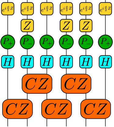
Figure 10: One layer of the circuit defined in Eq. 104, for a particular set of measurement outcomes. A circuit with $L_{y}$ such layers, with $P_{\pm}$ chosen according to the measurement outcomes for each row of the cluster state, results in $\ket{\Psi}_{\partial\mathcal{M}}$ – the state obtained after measuring the bulk qubits of a cluster state.

$H$ gate: The term $U^{\quantity{n}_{\tau+1},\quantity{n}_{\tau}}_{1}\outerproduct{\quantity{n}_{\tau+1}}{\quantity{n}_{\tau}}$ can be decomposed into a product of single particle operators

$$\prod\limits_{x}(-1)^{n_{x,\tau+1}n_{x,\tau}}\outerproduct{n_{x,\tau+1}}{n_{x,\tau}},$$ (107)

so it suffices to show that each single particle operator with matrix elements of the form $(-1)^{n_{x,\tau+1}n_{x,\tau}}$ corresponds to a $H$ gate. A single-qubit operator $U_{1}$ can be represented in the computational basis as

$$U_{1}\equiv\sum\limits_{n,n^{\prime}}\quantity(U_{1})_{n}^{n^{\prime}}\outerproduct{n^{\prime}}{n}.$$ (108)

By requiring the matrix elements of $U_{1}$ to be $\quantity(U_{1})_{n}^{n^{\prime}}=(-1)^{nn^{\prime}}$,

$$\quantity(U_{1})_{n}^{n^{\prime}}=\matrixquantity(1&1\\ 1&-1).$$ (109)

$U_{1}$ has the same representation as the Hadamard gate $H$, in the computational basis. This establishes the first connection in Eq. 105.

$CZ$ gate: Turning to the second term, we now construct a two-qubit unitary gate that is diagonal in the computational basis. It can similarly be represented as

$$U_{2}\equiv\sum\limits_{n,n^{\prime}}U_{2}^{n,n^{\prime}}\outerproduct{n,n^{\prime}}{n,n^{\prime}}.$$ (110)

Again, requiring $U_{2}^{n,n^{\prime}}=(-1)^{nn^{\prime}}$, $U_{2}$ has the same representation as the $CZ$ gate,

$$U_{2}\equiv\matrixquantity(1&&&\\ &1&&\\ &&1&\\ &&&-1)=CZ.$$ (111)

Weak Measurements: As with the $H$ gate, we consider a possibly non-unitary, diagonal, single-qubit operator $M$ whose representation is given by

$$M\equiv\sum\limits_{n}M^{n}\outerproduct{n}{n};$$ (112)

$$M^{n}\propto\frac{W^{n}}{\sqrt{1+|W|^{2}}}.$$

We reiterate the parametrization of $W$ according to Eqs. 3 and 4. This will also enable us to fix the normalization constant for $M$. For a single-qubit measurement performed in the direction $\hat{n}=\cos\theta\hat{z}+\sin\theta\cos\phi\hat{x}+\sin\theta\sin\phi\hat{y}$ with a measurement outcome $+\hat{n}$, the weight $W=\tan\frac{\theta}{2}e^{i\phi}$. The resulting operator $M_{+}$, constructed according Eq. 112, is

$$M_{+} \propto\frac{1}{\sqrt{1+\tan^{2}\frac{\theta}{2}}}\quantity(\outerproduct{0}{0}+e^{-i\phi}\tan(\frac{\theta}{2})\outerproduct{1}{1})$$ (113)

$$\propto\exp(i\frac{\phi}{2}Z)\quantity(\cos(\frac{\theta}{2})\outerproduct{0}{0}+\sin(\frac{\theta}{2})\outerproduct{1}{1})$$

$$\equiv\exp(i\frac{\phi}{2}Z)P_{+}(\beta).$$

where, in the last line, we have unambiguously defined the operator $M_{+}$. $P_{+}(\beta)$ refers to a weak projector (of strength $\beta$) to the $\ket{0}$ state

$$P_{+}(\beta)\equiv\frac{1}{\sqrt{2\quantity(1+\tanh^{2}(\beta))}}\quantity(1+\tanh(\beta)Z),$$ (114)

and the strength $\beta$ is defined via

$$\tanh(\beta)=\tan(\frac{\pi}{4}-\frac{\theta}{2}).$$ (115)

Similarly, when the outcome is $-\hat{n}$, the operator $M_{-}$ is defined as

$$M_{-} \propto\frac{1}{\sqrt{1+\cot^{2}\frac{\theta}{2}}}\quantity(\outerproduct{0}{0}-e^{-i\phi}\cot(\frac{\theta}{2})\outerproduct{1}{1})$$ (116)

$$\equiv\exp(i\frac{\phi}{2}Z)ZP_{-}(\beta),$$

where $P_{-}$ analogously refers to a weak projector to the $\ket{1}$ state

$$P_{-}(\beta)\equiv\frac{1}{\sqrt{2\quantity(1+\tanh^{2}(\beta))}}\quantity(1-\tanh(\beta)Z).$$ (117)

At their “strongest”, $P_{\pm}(\beta\to\infty)$ reduce to the projectors to the $\ket{0}$ and $\ket{1}$ states

$$P_{\pm}(\beta\to\infty)=\frac{1\pm Z}{2},$$ (118)

whereas at their weakest, $P_{\pm}(0)\propto 1$. Thus, these weak measurements generalize the idea of projective measurements, where weaker measurements (i.e., with smaller $\beta$) obtain less information from the system. $P_{\pm}$ describe a POVM and obey $P_{+}^{\dagger}P_{+}+P_{-}^{\dagger}P_{-}=1$. It follows that $M_{\pm}$ also constitute a valid set of Kraus operators since they are unitarily related to $P_{\pm}$; hence, $M_{\pm}(\beta)$ describe weak measurements followed by a single-qubit rotation about the Z axis.

The boundary state is now equivalent to a 1d state obtained after a hybrid quantum circuit of depth $L_{y}$, consisting of measurements and unitary operations, is applied to the state $\ket{+}^{\otimes L_{x}}$. The unitary gates in this circuit are dual unitary, and known to be maximally chaotic for generic $\phi$ [31, 32].

In conventional setups that have studied the MIPT in 1+1d random circuits, the tuning parameter is the rate $p$ at which projective measurements are performed on the qubits. In our interpretation, weak measurements are performed on every qubit at every time step, so $p=1$. However, an MIPT is observed even in such a setting [33]. The entanglement scaling of $\ket{\Psi}_{\partial\mathcal{M}}$ is expected to exhibit a transition from volume-law to area-law behavior as the strength $\beta$ is increased. An increase in $\beta$ is achieved by choosing the measurement axis to align closer to the Z axis (i.e. by decreasing $\theta$), according to Eq. 115. When $\theta=0\quantity(\beta=\infty)$, we expect an area-law scaling for $\ket{\Psi}_{\partial\mathcal{M}}$, whereas when $\theta=\frac{\pi}{2}\quantity(\beta=0)$, a volume-law scaling is expected, since the circuit is purely unitary (and chaotic). In subsequent sections, we present numerical evidence that a transition in the entanglement scaling behavior is observed as $\theta$ is varied. Using this mapping, the physics underlying this transition has been shown to be innately connected to the physics of MIPTs.

IV.4 Dynamics from Tensor Contractions

Another dynamical interpretation of this model is provided by considering its tensor network representation. While the method pioneered in [23] provides a generic algorithm to sample from 2D shallow circuits – such as the circuits used to prepare cluster states – we instead use a more direct method that utilizes the exact form of the tensors that constitute the cluster state, to construct the boundary state.

Certain 2D states, such as the cluster state, can be represented as a network of tensors [19, 34, 35], with each index of a tensor represented as a “leg”, with the understanding that legs that are connected correspond to indices that are summed over. Each tensor further has a physical index corresponding to the physical degrees of freedom, qubits, in our case. We distinguish these physical legs from the others by terming the latter “virtual” legs. The process of measuring a qubit in the Pauli $Z$ basis is equivalent to fixing a specific value $0$ or $1$ of its physical index, which effects a projection $\outerproduct{0}{0}$ or $\outerproduct{1}{1}$ on that qubit. Measurements in other bases can be implemented by applying an appropriate single-qubit rotation prior to constraining the value of the physical index. At the end of our protocol, the tensor only has physical legs at the top edge. The boundary state that remains after measuring the bulk qubits is obtained by contracting over all the remaining non-physical indices in the bulk of the network. However, owing to the associativity of tensor multiplication and the commutativity of projectors on different sites, we are free to choose the order in which the tensor network can be contracted to obtain the boundary state. A specific pattern of contractions, which can be interpreted as the evolution of a 1D state through a random nonunitary circuit, is described in the following paragraph and in Fig. 11. This procedure can be used to obtain the boundary state following any set of measurement outcomes $\quantity(\mu,\omega)$.

Concretely, we begin by considering the lowest row of the cluster state, defined on a square lattice with $L_{x}$ columns and $L_{y}$ rows. This row can be treated as an MPS $\ket{\psi_{\rm virt}(\tau=1)}$ where the $L_{x}$ virtual legs that connect this row to the next serve as physical legs. The tensors in the next row have virtual legs connected to tensors in rows both below and above them. They can be thought of as the Matrix Product Operator (MPO) decomposition of a nonunitary operator. We term this operator $T$, reminiscent of the transfer matrix from the previous section. The state $\ket{\psi_{\rm virt}}$ can now be “evolved” nonunitarily by contracting the legs it shares with $T$, and this process is iteratively continued over subsequent rows until the boundary state, i.e., the $L_{y}^{\rm th}$ row, is reached. The vertical direction can be reinterpreted as a discrete effective time direction. After $\tau\leq L_{y}-1$ such rows have been contracted – equivalently, $\tau$ “time steps” – the state is

$$\ket{\psi_{\rm virt}(\tau)}=\frac{\prod\limits_{\tau^{\prime}<\tau}T(\tau^{\prime})\ket{\psi_{\rm virt}}}{\norm{\prod\limits_{\tau^{\prime}<\tau}T(\tau^{\prime})\ket{\psi_{\rm virt}}}}.$$ (119)

The boundary state $\ket{\psi}_{\partial\mathcal{M}}$ is obtained by contracting $\ket{\psi_{\rm virt}}$ with the $L_{y}^{\rm th}$ row, resulting in an MPS with physical indices, as shown in Fig. 11.

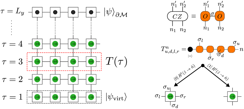
Figure 11: The process by which $\ket{\psi}_{\partial\mathcal{M}}$ is obtained on the square lattice. (Left) Each square represents a tensor of the form given in Eq. 133. The green circles denote outcomes (parallel or anti-parallel to the direction $\hat{n}$) for measurements performed on the bulk. The black circles represent the physical degrees of freedom of $\ket{\psi}_{\partial\mathcal{M}}$. (Right) The decomposition of $CZ$ into MPOs as given in Eq. 125, and the consequent iterative construction of $T^{n}_{u,l,d,r}$ starting from the $\ket{+}$ state.

IV.4.1 Obtaining Tensors for the Cluster State

The cluster state, as defined in Eq. 14, is obtained by applying $CZ$ gates across all pairs on neighboring qubits, all of which are initialized in the $\ket{+}$ state. We first derive the tensors for two neighboring qubits, labeled $1$ and $2$. Initially, $\ket{\psi}_{1}=\ket{+}_{1}$, $\ket{\psi}_{2}=\ket{+}_{2}$. Their joint wavefunction can be represented as

$$\ket{\psi}=\sum\limits_{n_{1},n_{2}=0,1}A^{n_{1}}A^{n_{2}}\ket{n_{1},n_{2}}$$ (120)

where $\ket{n_{1},n_{2}}$ is a state in the computational basis of the two qubits. The matrices $A^{n_{j}}=\frac{1}{\sqrt{2}}$ for $n_{j}=0,1$.

We proceed by obtaining a representation of the $CZ$ gate in terms of tensors as

$$CZ=\sum\limits_{\begin{subarray}{c}n_{1},n_{1}^{\prime}\\ n_{2},n_{2}^{\prime},\sigma\end{subarray}}O_{\sigma}^{n_{1}^{\prime},n_{1}}O_{\sigma}^{n_{2}^{\prime},n_{2}}\outerproduct{n_{1}^{\prime},n_{2}^{\prime}}{n_{1},n_{2}},$$ (121)

where $\sum\limits_{n_{j}^{\prime},n_{j}}O_{\sigma}^{n_{j}^{\prime},n_{j}}\outerproduct{n_{j}^{\prime}}{n_{j}}$ is an operator acting on the $j^{\rm th}$ qubit for each $\sigma$. After the application of the $CZ$ gate, the state

$$\ket{\psi}\to CZ\ket{\psi}=\sum\limits_{n_{1}^{\prime},n_{2}^{\prime},\sigma}B^{n_{1}^{\prime}}_{\sigma}B^{n_{2}^{\prime}}_{\sigma}\ket{n_{1}^{\prime},n_{2}^{\prime}}$$ (122)

where $B^{n_{j}^{\prime}}_{\sigma}=\sum\limits_{n_{j}}O_{\sigma}^{n_{j}^{\prime},n_{j}}A^{n_{j}}$. The action of the $CZ$ gate is given by

$$CZ\ket{n_{1},n_{2}}=(-1)^{n_{1}.n_{2}}\ket{n_{1},n_{2}}.$$ (123)

$CZ$ can equivalently be written as

$$CZ =P_{1}^{0}+P_{1}^{1}Z_{2}$$ (124)

$$=2\quantity(\frac{1+Z_{1}}{2})\quantity(\frac{1+Z_{2}}{2})-Z_{1}Z_{2}$$

$$=\matrixquantity(\sqrt{2}P_{1}^{0}\hfil&iZ_{1})\matrixquantity(\sqrt{2}P_{2}^{0}\\ iZ_{2}),$$

where $P^{0/1}_{j}\equiv\frac{1\pm Z_{j}}{2}$ is the projector onto $\ket{0}_{j}$or$\ket{1}_{j}$ and $Z_{j}$ is the Pauli $Z$ operator, both on the $j^{\rm th}$ qubit. From the last line, $O_{\sigma}^{n_{j}^{\prime},n_{j}}$ can be read off as

$$O_{\sigma}^{n_{j}^{\prime},n_{j}}=\begin{cases}\sqrt{2}\quantity(P^{0})^{n_{j}^{\prime},n_{j}},&\sigma=0\\ iZ^{n_{j}^{\prime},n_{j}},&\sigma=1\end{cases},$$ (125)

with $M^{n_{j}^{\prime},n_{j}}\equiv\matrixelement{n_{j}^{\prime}}{M}{n_{j}}$ for every 1-qubit operator $M$. Returning to the cluster state, the tensor corresponding to a vertex $v$, $T^{n}_{\sigma_{1},\sigma_{2},\dots,\sigma_{k}}$, whose neighbours are $v_{1},v_{2}\dots v_{k}$, and $\sigma_{j}$ labels the leg or index shared between $v$ and $v_{j}$, is given by

$$T^{n}_{\sigma_{1},\sigma_{2},\dots,\sigma_{k}}=\frac{1}{\sqrt{2}}\sum\limits_{\quantity{n_{j}}=0,1}O_{\sigma_{1}}^{n,n_{1}}O_{\sigma_{2}}^{n_{1},n_{2}}\dots O_{\sigma_{k}}^{n_{k-1},n_{k}}.$$ (126)

The unnormalized state of $T$ following a projective measurement is obtained by

$$\quantity(P^{0/1})^{n,n^{\prime}}\quantity(R^{\dagger}(\hat{z}\to\hat{n}))^{n^{\prime},n^{\prime\prime}}T^{n^{\prime\prime}}_{\sigma_{1},\sigma_{2},\dots,\sigma_{k}},$$ (127)

where $R\quantity(\hat{z}\to\hat{n})$ is the unitary operator effects a single-qubit rotation from the $\hat{z}$ to the $\hat{n}$ direction, for measurements performed along $\hat{n}$.

As an illustration, we provide a method by which the tensors for the cluster state on the infinite square lattice may be obtained. Let $T^{n_{x,y}}_{u_{x,y},d_{x,y},l_{x,y},r_{x,y}}(x,y)$ denote the tensor corresponding to the qubit located at the vertex $(x,y)$ of the square lattice. $n$ refers to the physical index, while $u,d,l$, and $r$ refer to virtual indices, respectively, the legs that point up, down, left, and right. The location dependence of these indices will be suppressed in their notation unless there is potential for ambiguity. From Eq. 126, with $O$ as in Eq. 125,

$$T^{n}_{u,d,l,r}=\frac{1}{\sqrt{2}}\sum\limits_{\quantity{n_{j}}=0,1}O_{u}^{n,n_{1}}O_{d}^{n_{1},n_{2}}O_{l}^{n_{2},n_{3}}O_{r}^{n_{3},n_{4}}.$$ (128)

This calculation of $T$ only needs to be performed once. Following this, the tensors for all other vertices are straightforwardly obtained by relabelling the indices to match the virtual indices of those vertices. By the geometry of the square lattice, the following indices are to be identified:

$$\begin{aligned} r_{x,y}&\leftrightarrow l_{x+1,y}\\ u_{x,y}&\leftrightarrow d_{x,y+1}\\ \end{aligned}.$$ (129)

Finally, the cluster state can be written as

$$\ket{\psi_{\rm G}} =\sum\limits_{\quantity{n_{x,y}}}\sum\limits_{\quantity{\begin{subarray}{c}u_{x,y},d_{x,y}\\ l_{x,y},r_{x,y}\end{subarray}}}$$ (130)

$$\quantity(\prod_{x,y}T^{n_{x,y}}_{u,d,l,r}(x,y)\delta_{r_{x,y},l_{x+1,y}}\delta_{u_{x,y},d_{x,y+1}})\ket{\quantity{n_{x,y}}},$$

with the Kronecker-$\delta$s enforcing the identification Eq. 129 in the summation. The last step in the protocol is the measurement of the bulk qubits, leaving behind the boundary state $\ket{\psi}_{\partial\mathcal{M}}$. We choose a uniform direction $\hat{n}$ along which all the bulk measurements are performed. With $\hat{n}$ fixed, the boundary state can uniquely be described by a collection of $L_{x}\times(L_{y}-1)$ bits $\quantity{s_{x,y}}$, where $s_{x,y}=0/1$ refers to a projective measurement resulting in a state parallel $\quantity(\ket{+\hat{n}})$ or anti-parallel $\quantity(\ket{-\hat{n}})$ to $\hat{n}$ at site $(x,y)$. This step is implemented in two substeps. First, we rotate each qubit using the unitary

$$\quantity(R^{\dagger}(\hat{z}\to\hat{n}))^{n_{x,y},n^{\prime}_{x,y}}\outerproduct{n_{x,y}}{n^{\prime}_{x,y}},$$ (131)

where $R(\hat{z}\to\hat{n})$ is the unitary operator that effects a rotation from the $\hat{z}$ axis to $\hat{n}$, as in Eq. 127. Next, we project that bulk qubit onto the state $\bra{s_{x,y}}$ by multiplying the tensor $T^{n}_{u,d,l,r}(x,y)$ by an appropriate vector $\quantity(P^{0,1})^{n}$, corresponding to a projection onto $\bra{0/1}$. The unnormalized boundary state $\ket{\psi}_{\partial\mathcal{M}}$ is finally given by

$$\ket{\psi}_{\partial\mathcal{M}}\propto\Biggl{(}\prod_{\quantity(x,y)\in{\rm bulk}}\quantity(P^{s_{x,y}})^{n_{x,y}}\quantity(R^{\dagger})^{n_{x,y},n^{\prime}_{x,y}}\times$$ (132)

$$T^{n^{\prime}_{x,y}}_{u,d,l,r}(x,y)\delta_{r_{x,y},l_{x+1,y}}\delta_{u_{x,y},d_{x,y+1}}\Biggr{)}$$

$$\quantity(\prod_{x,y=L_{y}}T^{n_{x,y}}_{d,l,r}(x,y)\delta_{r_{x,y},l_{x+1,y}}\ket{n_{x,y}}),$$

with the understanding that repeated indices are summed over. The absence of $u$ indices in the last line stem from the fact that the topmost row of the square lattice has no neighbors – and hence no virtual indices – above it.

IV.4.2 Implementing the 1+1D Circuit

The implementation of the 1+1D circuit that reproduces the boundary state of the square lattice once its bulk degrees of freedom have been measured can now be described in detail. We begin by noting that the expression for $\ket{\psi}_{\partial\mathcal{M}}$ in Eq. 132 consists of several tensor multiplications and will focus first on the terms in the first parentheses. Two types of multiplications are involved in this process – those involving contractions of the physical indices $n$ and those involving the virtual indices $\quantity{u,d,l,r}$. Crucially, the order in which these contractions are performed is irrelevant to the final solution, since matrix multiplication is associative. No contraction of the physical indices involves more than one site at a given time. By choosing the order of contractions, an interpretation of this process as a quantum circuit follows naturally. This can be demonstrated by considering the terms in the parentheses corresponding to the lowest row and subsequent rows separately. We proceed by expressing $\delta_{u_{x,y},d_{x,y+1}}$ as the inner-product of basis states as $\delta_{u_{x,y},d_{x,y+1}}\equiv\innerproduct{d_{x,y+1}}{u_{x,y}}$, and defining, for $1<y<L_{y}$,

$$T_{u,d,l,r}(x,y)\equiv\quantity(P^{s_{x,y}})^{n}\quantity(R^{\dagger})^{n,n^{\prime}}T^{n^{\prime}}_{u,d,l,r}(x,y),$$ (133)

and for $y=1$, since these tensors – being those on the last row of the lattice – do not have any virtual indices “below” them, as shown in Fig. 11,

$$B_{u,l,r}(x)\equiv\quantity(P^{s_{x,1}})^{n}\quantity(R^{\dagger})^{n,n^{\prime}}T^{n^{\prime}}_{u,l,r}(x,1).$$ (134)

The term in the first parentheses can be rewritten as

$$\prod_{x,1<y\leq L_{y}-1}T_{u,d,l,r}(x,y)\delta_{r_{x,y},l_{x+1,y}}\innerproduct{d_{x,y+1}}{u_{x,y}}\times$$ (135)

$$\prod_{x,y=1}B_{u,l,r}(x)\delta_{r_{x,1},l_{x+1,1}}\innerproduct{d_{x,2}}{u_{x,1}}.$$

The order of the bras and kets can be rearranged to give

$$\bra{d_{1,L_{y}}d_{2,L_{y}}\dots d_{L_{x},L_{y}}}$$ (136)

$$\quantity(\prod_{x,1<y\leq L_{y}-1}T_{u,d,l,r}(x,y)\delta_{r_{x,y},l_{x+1,y}}\outerproduct{u_{x,y}}{d_{x,y}})$$

$$\hskip 55.00008pt\quantity(\prod_{x,y=1}B_{u,l,r}(x)\delta_{r_{x,1},l_{x+1,1}}\ket{u_{x,y=1}}).$$

For each $1<y\leq L_{y}-1$, we can define an effective time-evolution operator $T(\tau)$ as

$$T(\tau)=\sum\limits_{\quantity{\begin{subarray}{c}u_{x,\tau},d_{x,\tau}\\ l_{x,\tau},r_{x,\tau}\end{subarray}}}\prod_{x}T_{u,d,l,r}(x,\tau)\delta_{r_{x,\tau},l_{x+1,\tau}}\outerproduct{u_{x,\tau}}{d_{x,\tau-1}},$$ (137)

and thus, express the terms in the first parentheses of Eq. 132 as an inner product $\innerproduct{d_{1,L_{y}}d_{2,L_{y}}\dots d_{L_{x},L_{y}}}{\psi_{\rm virt}(L_{y})}$, where

$$\ket{\psi_{\rm virt}(L_{y})}\equiv T(L_{y}-1)T(L_{y}-2)\dots T(2)\ket{\psi_{\rm virt}(\tau=1)}$$ (138)

$$\ket{\psi_{\rm virt}(\tau=1)}\equiv\quantity(\prod_{x,y=1}B_{u,l,r}(x)\delta_{r_{x,1},l_{x+1,1}}\ket{u_{x,y=1}}).$$

The vertical coordinate $y$ has been relabelled as an effective temporal direction $\tau$. The time evolution of $\ket{\psi_{\rm virt}}$ can equivalently be seen as an evolution of the $\quantity{B_{u,l,r}(x)}_{\tau}$, according to the rule

$$B_{u,\bar{l},\bar{r}}(x,\tau)=T_{u,l,d,r}(x,\tau)B_{u^{\prime},l^{\prime},r^{\prime}}(x,\tau-1)\delta_{d,u^{\prime}},$$ (139)

where $\bar{l}$ and $\bar{r}$ denote the combined indices $(l,l^{\prime})$ and $(r,r^{\prime})$ respectively.

To obtain the boundary state $\ket{\psi}_{\partial\mathcal{M}}$ at the final step of this dynamical evolution, the operator $T(\tau=L_{y})$, which maps the free virtual indices $\quantity{u_{x,y=L_{y}-1}}$ to the physical indices $\quantity{n_{x,y=L_{y}}}$, is given by the last line of Eq. 132 as

$$T(\tau=L_{y})=\prod_{x,y=L_{y}}T^{n_{x,y}}_{d,l,r}(x,y)\delta_{r_{x,y},l_{x+1,y}}\outerproduct{n_{x,L_{y}}}{d_{x,L_{y}}}.$$ (140)

The tensors for $T(\tau=L_{y})$ are those that constitute the top-most row of a cluster state on a square lattice. Their $d$ indices must be contracted with the $u$ indices of the MPS describing $\ket{\psi_{\rm virt}(\tau=L_{y}-1)}$ to obtain $\ket{\psi}_{\partial\mathcal{M}}$. Eq. 132 can finally be expressed as

$$\ket{\psi}_{\partial\mathcal{M}}\propto\prod\limits_{2\leq\tau\leq L_{y}}T(\tau)\ket{\psi_{\rm virt}(\tau=1)}.$$ (141)

We conclude this section by providing a brief algorithm that describes this implementation. Note that Eq. 137 describes the MPO representation of $T$, while Eq. 138 describes the MPS representation of the state $\ket{\psi_{\rm virt}}$. This identification allows us to use the extensively studied techniques for the time evolution of 1D quantum states.

1. Given a measurement direction $\hat{n}$, the measurement outcomes $\quantity{s_{x,y}}$, and the dimensions of the square lattice $L_{x}$ and $L_{y}$. Assume $L_{y}\geq L_{x}$.

2. Obtain the unitary gate $R$ which effects a rotation from $\hat{z}$ to $\hat{n}$

3. Calculate and store $B_{u,l,r}$ for both measurement outcomes $s=0,1$, using Eq. 134.

   • According to $\quantity{s_{x,y=1}}$, create an MPS for $\ket{\psi_{\rm virt}}$, where the tensors at site $x$ are $B^{(s_{x,y=1})}_{u,l,r}$.

   • Designate $u$ as a physical index, and relabel the virtual indices $l,r$ uniquely, ensuring, however, that $r_{x}=l_{x+1}$ (this enforces $\delta_{r_{x,y},l_{x+1,y}}$).

4. Calculate and store $T_{u,d,l,r}$ for either measurement outcome, using Eq. 133. These tensors $T_{u,d,l,r}(x,y>1)$ constitute the MPO representations of $T$.

   • Use standard techniques [35, 36] to “time-evolve” (and truncate, if necessary) the MPS $\ket{\psi_{\rm virt}}$.

   • Normalize the state $\ket{\psi_{\rm virt}}$.

   • Repeat this process for $\tau=L_{y}-1$ time-steps.

5. Evolve the state with $T(\tau=L_{y})$ to obtain $\ket{\psi}_{\partial\mathcal{M}}$.

V Numerical Results

We now turn to the numerical characterization of the boundary state obtained after performing single-qubit measurements on all the qubits in the bulk of a 2D graph state. We consider two types of bulk measurements: (A) measurements in arbitrary directions, and (B) Pauli X/Y/Z measurements. Broadly, in (A), we vary the direction along which the measurements are performed, whereas in (B), we alter the fraction of X/Y/Z measurements. We are specifically interested in determining the presence of an entanglement transition as these parameters are varied. We further seek to establish connections between the entanglement of the boundary state and the difficulty of approximating certain families of partition functions.

V.1 Entanglement Scaling at Arbitrary Measurement Directions

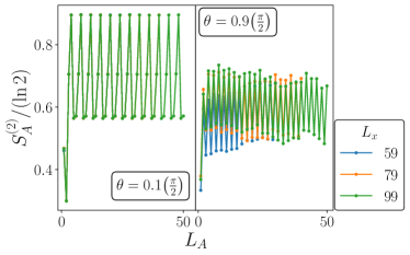
Figure 12: The entanglement entropy in the boundary state of a Lieb lattice with dimensions $L_{y}=500$ and $L_{x}$. Measurements are performed along $\hat{n}=\cos(\theta)\hat{z}+\sin(\theta)\hat{x}$. In both cases, $S_{A}$ shows no dependence on subsystem-size $L_{A}$, nor does it change with $L_{x}$, indicating an area-law phase.

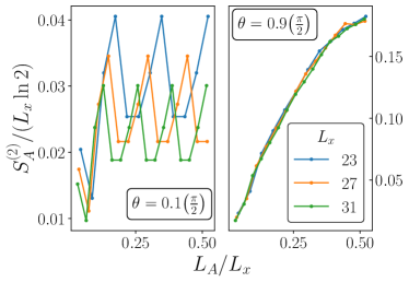
Figure 13: The scaling of entanglement entropy in the boundary state of a Lieb lattice with dimensions $L_{y}=500$ and $L_{x}$. Measurements are now performed along $\hat{n}=\cos(\theta)\hat{z}+\sin(\theta)\hat{y}$. (Left) $S_{A}/L_{x}$ trends downward as $L_{x}$ increases, indicating that the entanglement scales sub-linearly. When $S_{A}$ is plotted as a function of $L_{A}$ (as in Fig. 12, not shown), the curves superimpose one-another, indicating an area-law phase. (Right) $S_{A}$ scales linearly with $L_{x}$, and the data is amenable to a collapse indicative of a volume law phase.

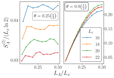
Figure 14: The scaling of entanglement entropy in the boundary state of a square lattice with dimensions $L_{y}=500$ and $L_{x}$. Measurements are performed along $\hat{n}=\cos(\theta)\hat{z}+\sin(\theta)\hat{x}$. As in Fig. 13, (Left) $S_{A}/L_{x}$ trends downward as $L_{x}$ increases, while (Right) $S_{A}$ scales linearly with $L_{x}$, indicating a volume law phase.

Results are presented here for the entanglement of the boundary state after forced measurements are performed along an arbitrary direction $\hat{n}$ on the qubits in the bulk. The entanglement is quantified using the $2^{\rm nd}$ Rényi entropy $S^{(2)}_{A}$, defined as

$$S^{(2)}_{A}=-\ln\tr\rho^{2}_{A},$$ (142)

where $\rho_{A}=\tr_{\overline{A}}\outerproduct{\psi_{\rm edge}}{\psi_{\rm edge}}$ is the reduced density matrix describing subsystem $A$ of the boundary state $\ket{\psi}_{\partial\mathcal{M}}$, and $\overline{A}$ is the complement of $A$.

We consider the cluster state defined on (1) the Lieb lattice and (2) the square lattice as initial states. Our simulation emulates the following setup – on the initial state, a single qubit measurement is performed on the qubit located at position $\vec{r}$, along the (possibly position-dependent) direction $\hat{n}(\vec{r})$. Following a measurement, the qubit points along $\hat{n}$ or $-\hat{n}$. The outcome, however, is “post-selected”, in that the outcome is chosen with a predetermined probability distribution; the specific distributions will be described later in this section.

We denote by $L_{x}$ the horizontal width of the lattice, and by $L_{y}$, its vertical length. By employing the tensor network scheme described in Section IV.4, these dimensions have the alternate interpretation of $L_{x}$ qubits undergoing a nonunitary, stroboscopic evolution for $L_{y}$ “time steps”. Since the accessible horizontal sizes are limited in numerical simulations, we use the following criteria to determine the entanglement scaling behavior: for a given $\hat{n}$, we first plot the scaled entanglement entropy $S_{A}/L_{x}$ as a function of fractional subsystem size $L_{A}/L_{x}$ for various sizes $L_{x}$. If the curves approximately collapse onto a single curve, the boundary state obeys a volume-law scaling ,$S^{(2)}_{A}\sim|A|$, and is hard to simulate using a tensor network scheme. If the curves instead trend downward with increasing $L_{x}$, this signals an area-law scaling, $S^{(2)}_{A}\sim{\rm const}$, of the entanglement entropy, and the boundary state is easily simulable. These simulations were implemented using the ITensor Julia package [36, 37].

In this section, we first explore the effects of uniformly measuring all the bulk qubits along a direction $\hat{n}(\vec{r})\equiv\hat{n}$, independent of their position. $\hat{n}$ is parameterized by the angles $\theta$ and $\phi$ as $\hat{n}=\cos\theta\hat{z}+\sin\theta\cos\phi\hat{x}+\sin\theta\sin\phi\hat{y}$. The outcomes at each site are chosen independently and randomly to be $\pm\hat{n}$ with equal probability, and $S^{(2)}_{A}$ for the boundary state is finally averaged over 20 such sets of outcomes, so as to ameliorate the noise, and bring the underlying scaling with $|A|$ to the fore. We believe that our results capture the typical behavior of the boundary states, despite this post-selection. For the cluster state defined on the Lieb lattice, we separately consider the cases where $\hat{n}$ lies in X-Z plane ($\phi=0$), and in the Y-Z plane ($\phi=\frac{\pi}{2}$), whereas in the square lattice, we only consider the case where $\phi=0$.

Under certain conditions, we find that the entanglement of the boundary state undergoes a phase transition as the measurement angle $\theta$ is varied. This is interesting in its own right, since this transition adds to the panoply of measurement-induced phase transitions. Additionally, such a transition also bears interesting consequences for the feasibility of using an effective 1+1D dynamics to approximate the partition functions of 2d Ising models. As described in Section III, every boundary state has an associated classical Ising partition function $\mathcal{Z}$. In the area-law phase, $\mathcal{Z}$ can be computed efficiently for large system sizes with controlled approximations, but in the volume-law phase, these approximations to $\mathcal{Z}$ are uncontrolled, and thus, the calculations of $\mathcal{Z}$ requires resources exponentially large in $L_{x}$. In the 1+1D dynamics, the approximations correspond to retaining only a fixed number of the largest singular values in each of the tensors that constitute $\ket{\psi_{\rm virt}}$. This can be done with a controlled error only if $\ket{\psi_{\rm virt}}$ is area-law entangled.

We further utilize this connection to explore the complexity of approximating partition functions of specific classical models. This proceeds by restoring the position dependence of $\hat{n}(\vec{r})$ and postselecting for the $+\hat{n}(x,y)$ outcome. The measurement protocols that we consider correspond to classical Random Bond Ising Models (RBIMs), as in Eqs. 53 and 56. We begin by studying RBIMs where the absolute values of the interaction parameters ($|K|$) are fixed to be constant, but their signs ($K/|K|$) take random values $\pm 1$ for each set of interacting spins. The magnetic field $h$ is taken to be a constant as well. We proceed to study a few different types of coupling, and thereby attempt to uncover the factors that could play a key role in making the calculation of partition functions hard.we posit that the complexity of calculating $\mathcal{Z}$ (using a 1+1D-like algorithm) depends crucially on the form of the interactions in the Hamiltonian of $\mathcal{Z}$.

V.1.1 Lieb Lattice

In the Lieb lattice, a volume-law entangled phase is absent in the boundary state of a Lieb lattice when $\hat{n}$ lies in the $X$-$Z$ plane. $\hat{n}$ is parameterized by the angle $\theta$ that it makes with the z-axis, as $\hat{n}\equiv\cos{\quantity(\theta)}\hat{z}+\sin{\quantity(\theta)}\hat{x}$. In this case, the boundary state is always area-law entangled. The $\mathcal{Z}$ corresponding to this case has positive and negative weights, but we see that this does not lead to a change in the complexity of its calculation. When $\hat{n}$ is instead chosen to lie in the $Y-Z$ plane, now parameterized as $\hat{n}\equiv\cos{\quantity(\theta)}\hat{z}+\sin{\quantity(\theta)}\hat{y}$, an area-law to volume-law transition is observed as $\theta$ is tuned through $\theta_{c}\sim 0.75\quantity(\frac{\pi}{2})$. $\mathcal{Z}$ now includes complex weights, but it is only above a specific value of $\theta$ that this calculation becomes hard.

V.1.2 Square Lattice

In contrast to the Lieb lattice, we find an area- to volume-law transition in the scaling of the entanglement entropy of the boundary state in the square lattice, even as $\hat{n}$ is varied in the X-Z plane. For small $\theta$, the state is area-law entangled, but becomes volume-law entangled as $\theta$ exceeds $\theta_{c}\sim 0.7\frac{\pi}{2}$. Again, here, $\mathcal{Z}$ is entirely of real weights, but the corresponding Ising model now has 4-body interactions Eq. 56, as opposed to 2-body interactions in the Lieb lattice. Using the mapping Eq. 56, we can obtain the following intuition for the transition. When $\theta=0$, the (real part of) Ising interaction strength is $0$, while the contribution from the magnetic field to the partition function is 0, unless all the outcomes are $-$. In the opposite limit $\theta=\frac{\pi}{2}$, the Ising interactions are equally likely to be $\pm\infty$. The increasing relevance of the frustrations arising from the 4-body interactions as $\theta$ is varied could be responsible for the poor performance of the 1+1D algorithm.

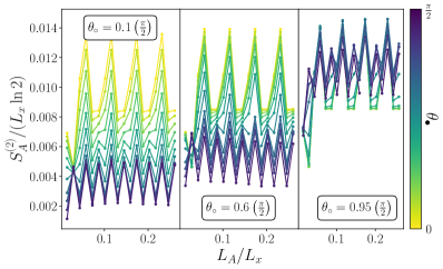
Figure 15: $S^{(2)}_{A}$ for $\ket{\psi}_{\partial\mathcal{M}}$ obtained after measurements on the Lieb lattice, for different values of $\theta_{\bullet}$ and $\theta_{\circ}$. The measurement outcomes are post-selected to be $+\hat{n}_{\circ/\bullet}$, where $\hat{n}$ lies in the X-Z plane on both $\circ$ and $\bullet$ sublattices. $\theta_{\circ}$, which sets the magnetic field in $\mathcal{Z}$, is held constant, while only $|\theta_{\bullet}|$ is fixed (i.e. $\hat{n}$ is randomly chosen to make an angle $\pm\theta_{\bullet}$ with the $Z$ axis). The boundary state is always in an area law, indicating that the associated Ising partition function, with 2-spin random interactions on the square lattice, consists only of positive weights and is easy to approximate.

Randomness in the measurement outcomes is crucial to observing any non-area-law phase on the square lattice. If the measurement outcomes are all chosen to be equal ($+1$, for instance), the boundary state is area-law entangled in the thermodynamic limit $L_{y}\to\infty$. The finite-size scaling of entanglement is shown in the presence and absence of randomness in Fig. 16, in the square lattice, making evident the significance of stochasticity. Frustration is important to making the calculation of $\mathcal{Z}$ hard, and cannot exist if all measurement outcomes and directions – consequently, the Ising interaction strengths – are the same. This explains the differences between our results and those found in [38], where the boundary state obtained after measurements on the square lattice is never in a volume-law phase, except at $\theta=\frac{\pi}{2}$.

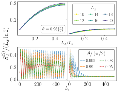
Figure 16: Entanglement entropy density of the boundary state when the measurement outcomes of the bulk are (left) random and (right) fixed to be along $+\hat{n}$. The greater entanglement when there is randomness in the measurement outcomes is accompanied by a higher degree of frustration in the corresponding classical model. (Top) Scaling of $S_{A}$ as a function of subsystem size for different $L_{x}$ (Bottom) “Evolution” of the entanglement of the boundary state with vertical depth $L_{y}$ (or imaginary time $\tau$). In the absence of randomness, $S^{(}2)_{A}$ decays strongly, ultimately saturating in values much smaller than in the case with randomness as $L_{y}\to\infty$.

V.1.3 Connections to Classical Partition Functions

We have, thus far, discussed the entanglement scaling as the measurement direction is kept uniform across the lattice, while outcomes are random. We have also demonstrated that the resulting boundary state $\ket{\psi}_{\partial\mathcal{M}}$ can be described in terms of a classical parition function $\mathcal{Z}$. In this subsection, we instead use a different type of post-selected measurement outcomes to glean information about the computational complexity of the corresponding $\mathcal{Z}$ that describes the $\ket{\psi}_{\partial\mathcal{M}}$. We focus on the specific cases of $\mathcal{Z}$ that describe RBIMs, where the randomness is only in the sign of the Ising interaction. The implementation is described below.

We begin by considering the case where the measurement outcomes are all $+1$, meaning that the measurement outcomes all point along $\hat{n}(x,y)$, but $\hat{n}$ can now be position-dependent. We also choose $\hat{n}$ to lie in the X-Z plane (so $\phi=0$). From Eq. 24, we see now that the $K$ and $h$ parameters are given by

$$\exp(-2h_{k})=\tan\quantity(\theta_{\circ}/2) \quad k\in\circ$$ (143)

$$\exp(-2K_{i})=\frac{1-\tan\quantity(\theta_{\bullet}/2)}{1+\tan\quantity(\theta_{\bullet}/2)} \quad i\in\bullet$$

Given a value of the magnetic field $h_{k}$ at site $k$, we can instead set that term to be $-h_{k}$ by setting $\theta_{\circ}\to\pi-\theta_{\circ}$. This, in turn, ensures that the $\mathcal{Z}$ that describes $\ket{\psi}_{\partial\mathcal{M}}$ has the magnetic field at site $k$ flipped.

Similarly, to toggle only the sign of the interaction $K_{i}$ from $+$ to $-$, only the change $\theta_{\bullet}$ to $-\theta_{\bullet}$ needs to be effected. We then consider an evolution where the measurement outcomes are all chosen to be $+1$, but the angle is drawn randomly from $\quantity{\theta_{\bullet},-\theta_{\bullet}}$ with equal probability. These angles are independently drawn for each site on the $\bullet$ sublattice. This models interactions of the form

$$|K|\sum_{\expectationvalue{i,j}}{\rm sign}\quantity(K_{ij})s_{i}s_{j}$$ (144)

in the Lieb lattice, and

$$|K|\sum_{i\in\bullet}{\rm sign}\quantity(K_{i})s_{a}s_{b}s_{c}s_{d}$$ (145)

in the square lattice. As in Eq. 30, $s_{a},s_{b},s_{c}$ and $s_{d}$ refer to the 4 sites belonging to the $\circ$ sublattice that enclose site $i$. The sign of the coupling ${\rm sign}\quantity(K)=\pm 1$ corresponds to $\hat{n}=\quantity(\cos\theta)\hat{z}\pm\quantity(\sin\theta)\hat{x}$. Measurements on the $\circ$ sublattice are performed along a fixed direction $\hat{n}$ and the outcomes are fixed to be +1, corresponding to a $\mathcal{Z}$ with a fixed magnetic field.

In the Lieb lattice, we find that the state is always in an area-law, as shown in Fig. 15, which suggests that the partition function of an RBIM with 2-body interactions should always be easily approximated, independent of $\theta$ (or $|K|$). Surprisingly, we find this to be the case in the square lattice as well. The plots presented in Fig. 17 show that $\ket{\psi}_{\partial\mathcal{M}}$ is found to obey an area law, unlike in the case with randomized measurement outcomes. Using the results of our numerical simulations, we are able to make the following claims about when the process of approximating $\mathcal{Z}$ (or equivalently, sampling from the cluster state in arbitrary measurement directions $\hat{n}$) becomes hard, for the specific interactions that we have considered in this work.

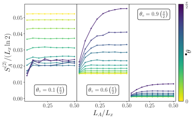
Figure 17: $S^{(2)}_{A}$ for $\ket{\psi}_{\partial\mathcal{M}}$ obtained after measurements on the square lattice. The set up is identical to that used for Fig. 15. The associated Ising partition function, with 4-spin random interactions on the square lattice, but still consisting only of positive weights, is also easy to approximate.

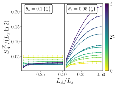
Figure 18: $S^{(2)}_{A}$ for $\ket{\psi}_{\partial\mathcal{M}}$ obtained after measurements on the square lattice. Unlike in Fig. 17, $\theta_{\bullet}$ is held fixed, but the measurement outcomes are now randomly chosen to be $\pm\hat{n}$, but only on the $\bullet$ sublattice. The boundary state entanglement now shows an area- to volume-law transition provided $\theta_{\circ/\bullet}$ are sufficiently high. The associated $\mathcal{Z}$ is now composed of both positive and negative weight terms. This suggests the necessity of negative weights in observing a transition in the complexity of approximating $\mathcal{Z}$.

When $\theta_{\bullet}$ is either $\pm\theta$, with the $+\hat{n}$ outcome post-selected and $0\leq\theta\leq\frac{\pi}{2}$, the corresponding weights in $\mathcal{Z}$ are always positive. Since the boundary state is in an area law regardless of the number of spins that participate in each interaction (2 in the Lieb lattice, 4 in the square lattice), we posit that positive weights with such interactions lead to a partition function whose approximation is always easy.

With a fixed $\theta$, $0\leq\theta\leq\frac{\pi}{2}$, negative weights in $\mathcal{Z}$ correspond to a measurement outcome along $-\hat{n}$, since in this case, Eq. 143 is modified to give the following relations

$$\exp(-2h_{k})=-\cot\quantity(\theta_{\circ}/2) \quad k\in\circ$$ (146)

$$\exp(-2K_{i})=-\frac{1+\tan\quantity(\theta_{\bullet}/2)}{1-\tan\quantity(\theta_{\bullet}/2)} \quad i\in\bullet$$

In the square lattice, we showed earlier that in the presence of randomness in the measurement outcomes, i.e. both $\pm\hat{n}$ outcomes are possible, a volume-to-area-law transition is observed. From Eq. 146, this corresponds to a $\mathcal{Z}$ with negative weights. Intriguingly, such a transition is observed, as shown in Fig. 18, even when the measurement outcomes are identical on one sublattice ($\circ$, in this case), provided there is randomness in the measurement outcomes on the other sublattice ($\bullet$). This indicates that a finite density of negative weights can make the approximation of $\mathcal{Z}$ hard.

Lastly, measurements performed along $\hat{n}$ lying in the X-Z plane, on a graph state on the Lieb lattice, always result in an area law phase for the boundary state. Thus, approximating $\mathcal{Z}$ for a 2D Ising model with 2-body interactions only becomes hard in the presence of complex weights. This is the case even in the absence of randomness in the measurement outcomes, provided $\theta>\theta_{c}$.

In summary, partition functions describing these specific interactions and with positive weights appear easy to approximate. Negative weights in $\mathcal{Z}$ can lead to a transition in the complexity of its approximation with 4 body interactions, but evidently not with 2 body interactions. The presence of complex weights generically can cause a transition, provided the real parts of the interaction strengths $K$ (or equivalently, the magnitude of the weights) are above a certain value.

We conclude this subsection by noting that the results presented so far pertained specifically to a sampling algorithm obtained by treating a 2D quantum state sampling problem as an effective 1+1D nonunitary dynamics. However, these results do not forestall the existence of an algorithm that could nonetheless circumvent these difficulties; we only find that the boundary evolution algorithm fails under these circumstances.

V.2 Entanglement Scaling with Random Pauli Measurements

This section investigates the boundary entanglement structure induced by bulk Pauli measurements on a $2$d cluster state. We first review the dynamical method introduced in our previous work [24].

For a cluster state defined on a 2D lattice, the measurement in one row will only affect its neighboring rows. Consequently, in the process of generating the boundary state at the top row, we can exchange the orders of CZ gates and single qubit measurements. Drawing inspiration from this insight, we design the algorithm as follows: We first prepare a three-layer cluster state, perform Pauli measurement in the middle layer, and remove the measured qubits. Next, we use the CZ gates to entangle the remaining two-layer state with an additional third layer of cluster state. Iterating this process and, at the final time, measuring all the non-boundary qubits, we thus obtain the boundary state $\ket{\Psi}_{\mathcal{M}}$ by avoiding the need for the construction of the 2D cluster state. This method is similar to the dynamical tensor contractions employed in the preceding section.

V.2.1 Volume-law-area-law Transition

We consider the cluster state defined on the Lieb lattice and perform randomized Pauli $X$, $Y$, and $Z$ measurements on the bulk qubits with probabilities $p_{x}$, $p_{y}$, and $p_{z}$, respectively, restricted by

$$p_{x}+p_{y}+p_{z}=1.$$ (147)

For simplicity we only consider the ”rough” boundary on the bottom discussed in Sec. IV. We first investigate the scaling of the n-Rényi entropy

$$S_{A}^{n}=\frac{1}{1-n}\ln\tr\rho_{A}^{n}$$ (148)

on the boundary. Here $\rho_{A}=\tr_{\overline{A}}\rho$ is the partial trace of the density matrix of the boundary state $\rho=\ket{\Psi}_{\partial\mathcal{M}}\bra{\Psi}_{\partial\mathcal{M}}$. As a consequence, the post-measurement boundary state is still a stabilizer state, whose entanglement entropy is independent of Rènyi index $n$. We thus drop the index $n$ in the following parts of this section. Without the $Y$ measurement, the boundary $1$d state is area-law entangled with $S_{A}\sim\text{const.}$. However, as shown in Fig. 19, when the $Y$ measurement dominates, the entanglement entropy satisfies volume-law scaling, $S_{A}\sim L$ with $L_{A}=1/2L$. By adjusting the measurement rate $p_{y}$, we induce an entanglement transition from the volume-law phase to the area-law phase. This transition can be mapped to MIPT by the transfer matrix formalism presented in Sec. IV.1, where we demonstrate that $X$ or $Z$ measurements correspond to one or two-qubit projective measurements. In contrast, the $Y$ measurements correspond to entangling unitary gates. The interplay between the entangling $Y$ measurement and the disentangling $X/Z$ measurement drives the entanglement phase transition. In the following part of this section, we take $L$ as the number of qubits on the boundary $\partial\mathcal{M}$, and $L_{A}$ as the number of qubits in subsystem $A$.

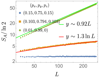
Figure 19: Entanglement entropy $S_{A}$ of the fixed ratio $L_{A}/L=1/2$ vs. boundary length $L$ for the boundary state of the Lieb graph state.

The position of the volume-law to area-law entanglement phase transition can be determined by identifying the peak of the mutual information [3]

$$I_{AB}=S_{A}+S_{B}-S_{AB}$$ (149)

of two antipodal regions $A$ and $B$ on the boundary $\partial\mathcal{M}$ with $L_{A}=L_{B}=L/8$ as shown in Fig. 21. Employing this method, we construct the phase diagram presented in Fig. 20.

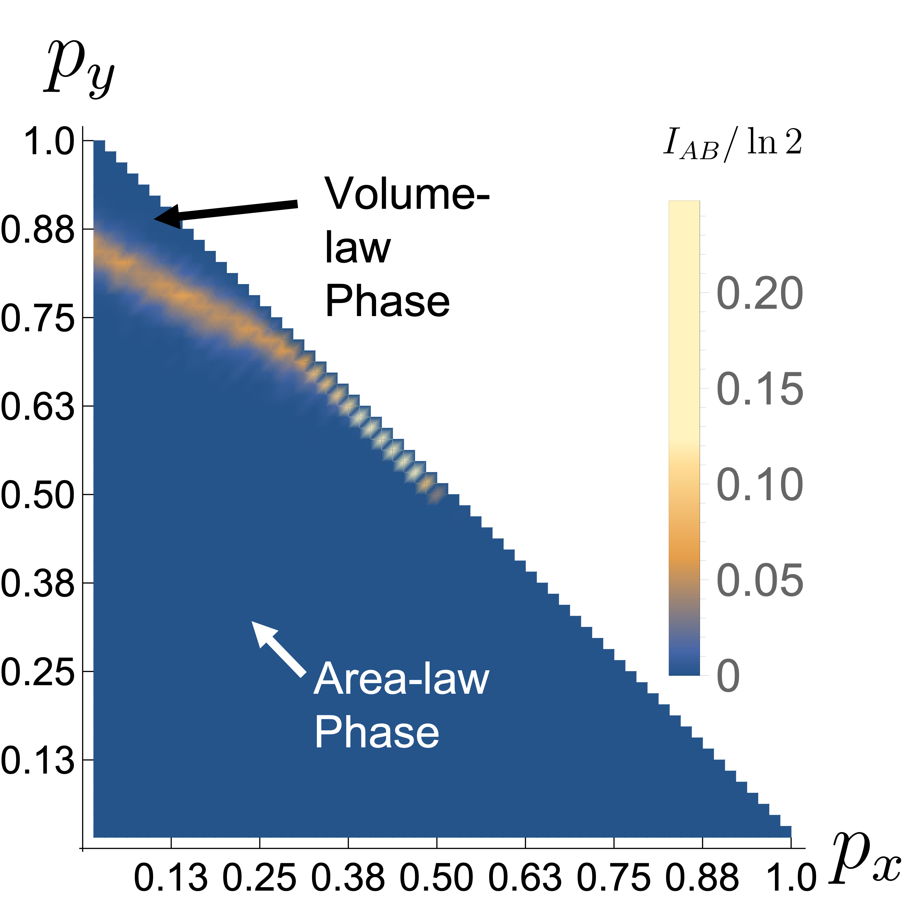
Figure 20: (Lieb lattice model) Mutual information $I_{AB}$ of antipodal domains $A$ and $B$, with $L_{A}=L_{B}=L/8$. The yellow line (mutual information peak) marks the phase boundary.

We further explore the entanglement phase transition of the two specific cases: (1) when $p_{z}=0$, allowing only $X$ and $Y$ measurements, and (2) when $p_{x}=0$, with only random $Z$ and $Y$ measurements.

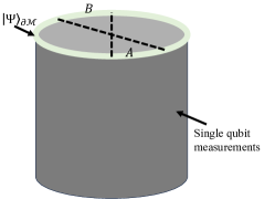
(a) Geometry of subsystem $A,B$, $L_{A}=L_{B}=L/8$

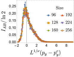
(b) Mutual information data collapse for $p_{z}=0$, where $p_{y}^{c}=0.58$, $\nu=1.78$

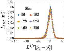
(c) Mutual information data collapse for $p_{x}=0$, where $p_{y}^{c}=0.858$, $\nu=1.3$

Figure 21: Mutual Information data collapse $I_{AB}=f(L^{1/\nu}(p_{y}-p_{y}^{c}))$ for the critical points of the boundary state defined on the Lieb graph state.

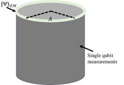
(a) Geometry of subsystem $A$

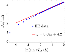
(b) $p_{z}=0$, $p_{y}=p_{y}^{c}=0.58$, $p_{x}=0.42$

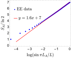
(c) $p_{x}=0$, $p_{y}=p_{y}^{c}=0.858$, $p_{z}=0.142$

Figure 22: The entanglement entropy scaling of Lieb lattice model at the critical points, with $L=256$

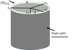
(a) Geometry of subsystem randomly chosen disjoint $A$, $B$

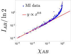
(b) $p_{z}=0$, $p_{y}=p_{y}^{c}=0.58$, $p_{x}=0.42$

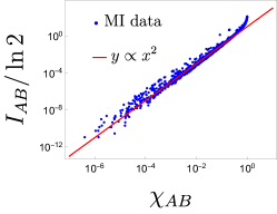
(c) $p_{x}=0$, $p_{y}=p_{y}^{c}=0.858$, $p_{z}=0.142$

Figure 23: Critical mutual information (MI) scaling of Lieb lattice model, $I_{AB}\sim\chi_{AB}^{\Delta}$

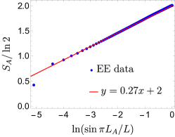
(a) Critical entanglement scaling, $p_{x}=p_{z}=0.5$, $p_{y}=0$

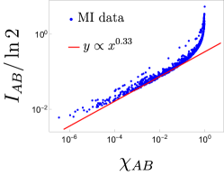
(b) Critical mutual information scaling, $p_{x}=p_{z}=0.5$, $p_{y}=0$

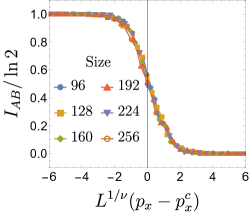
(c) Mutual information data collapse at $p_{y}=0$, $p_{x}^{c}=0.5$, $\nu=3/4$

Figure 24: Criticality of the area-law phase to the area-law phase transition at $p_{y}=0$, $p_{z}=p_{x}=0.5$.

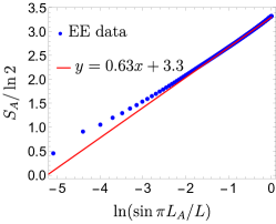
(a) $p_{x}=p_{z}=0.4$, $p_{y}=0.2$

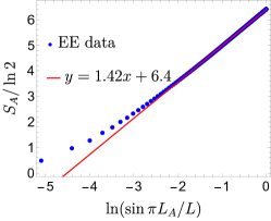
(b) $p_{x}=p_{z}=0.2$, $p_{y}=0.6$

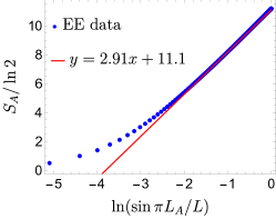
(c) $p_{x}=p_{z}=0.1$, $p_{y}=0.8$

Figure 25: Logarithmic scaling of entanglement entropy in the critical Goldstone phase with system size $L=512$.

For $p_{z}=0$, where only $X$ and $Y$ Pauli measurements exist, the criticality is observed at $p_{y}=0.58$ and $p_{x}=0.42$. The mutual information of two antipodal regions peaks at the critical point and collapses to

$$I_{AB}\sim f\big{(}L^{1/\nu} (p_{y}-p_{y}^{c})\big{)}$$ (150)

$$p_{y}^{c}=0.58, \quad\nu=1.78.$$

as shown in Fig. 21b. At criticality, the entanglement entropy scales logarithmically with subsystem size $L_{A}$

$$S_{A}/\ln 2\sim 0.58\ln\sin(\pi\frac{L_{A}}{L})$$ (151)

which is shown in Fig. 22b. At criticality, the mutual information $I_{AB}$ of two disjoint regions $A$ and $B$ is a function of the cross-ratio $\chi_{AB}$. In particular, when $\chi_{AB}$ is close to zero, as shown in Fig. 23b, we have

$$I_{AB}\sim\chi_{AB}^{0.6}$$ (152)

with

$$\chi_{AB}=\frac{x_{12}x_{34}}{x_{13}x_{24}},\quad\mbox{with}~{}x_{ij}=\frac{L_{x}}{\pi}\sin\left(\frac{\pi}{L_{x}}|x_{i}-x_{j}|\right),$$ (153)

where $x_{i=1,2,3,4}$ are endpoints of subregions $A$ and $B$ as shown in Fig. 23a.

Taking $p_{x}=0$, the critical point occurs at $p_{y}=0.858$ and $p_{z}=0.142$. Fig.22c showing that $S_{A}/\ln 2\sim 1.6\ln(\sin(\pi L_{A}/L))$. The mutual information $I_{AB}$ data collapse around the critical point is shown in Fig. 21c, where we have $\nu=1.3$. Furthermore, at criticality, Fig. 23c presents the scaling of mutual information between two disjoint intervals $A$ and $B$, characterized by $I_{AB}\sim\chi_{AB}^{2}$ with small $\chi$.

V.2.2 Absence of the volume-law phase

As demonstrated in Eq. 27, measuring all the vertex qubits along the $X$-direction on the Lieb lattice allows us to generate the toric code state up to some Pauli rotations. We further perform randomized Pauli $X$, $Y$, and $Z$ measurements in the bulk edge qubits of the Lieb lattice cluster state with probabilities $p_{x}$, $p_{y}$, and $p_{z}$, respectively. Using the transfer matrix method detailed in Sec. IV.2.2, we can show that this dynamics is equivalent to a free fermion system subject to repeated projective measurements as reported in [17]. Similar physics has recently been discussed in Ref. [30]. The $Y$ measurement generates a unitary free fermion gate, effectively braiding a pair of Majorana fermions, while the $X$ and $Z$ measurements correspond to $X$ and $ZZ$ measurements in the effective $1+1$d dynamics, respectively. This non-unitary free fermion dynamics can be mapped to a loop model, which has been extensively studied in Ref. 39.

When the $Y$ measurement dominates, a critical phase emerges. Its entanglement entropy scales like this

$$S_{A}/\ln 2\sim\alpha\ln\sin\left(\frac{\pi L_{A}}{L}\right)+$$ (154)

$$\mathcal{O}\bigg{(}\ln^{2}\sin\left(\frac{\pi L_{A}}{L}\right)\bigg{)},$$

with $\alpha$ being some non-universal constant varying with measurement rate $p_{x},p_{y},p_{z}$. Some entanglement entropy scaling data with $p_{x}=p_{z}=(1-p_{y})$ are shown in Fig. 25.

For nonzero $p_{y}$, varying $p_{x}$ or $p_{z}$ can induce transitions between the area-law and critical phases. In the limit $p_{y}=0$, the intermediate critical phase disappears. Consequently, varying $p_{x}$ results in a direct area-law to area-law transition, with the critical point described by the 2D percolation conformal field theory[40]. This result is confirmed by us numerically. At criticality, as illustrated in Fig. 24a, the entanglement entropy scales as:

$$S_{A}/\ln 2\sim\frac{K}{2}\ln\sin\left(\frac{\pi L_{A}}{L}\right),$$ (155)

where $K=0.54\approx\sqrt{3}/\pi$, which agrees with the theoretical prediction [39, 40]. The critical scaling of the mutual information is given by:

$$I_{AB}\sim\chi_{AB}^{\Delta},\quad\Delta=0.33\sim\frac{1}{3},$$ (156)

as shown in Fig. 24b. Furthermore, we examine the data collapse of the mutual information for two antipodal intervals, $A$ and $B$, with $L_{A}=L_{B}=L/4$. The mutual information collapses to

$$I_{AB}\sim g(L^{1/\nu}(p_{x}-p_{x}^{c}))$$ (157)

with $\nu=3/4$ and $p_{x}^{c}=0.5$, which can be identified as a bond percolation on a square lattice, which agrees with the result shown in Ref. 17.

The two area-law phases can be further characterized by their difference in the mutual information $I_{AB}$. Notably, we consider $L_{A}=L_{B}=L/4$ and the domain distance $r_{AB}=L/2$. The phase diagram is presented in Fig. 26. In one phase, we have $I_{AB}=0$. Conversely, in the other phase, the system displays long-range entanglement characterized by $I_{AB}=\ln 2$. This arises from the logical operator $O_{L}=\prod_{i\in l_{n}}X_{i}$ of the parent toric code state, where $l_{n}$ denotes the non-contractable loop of the cylinder. When the bulk $Z$ measurement on the edge qubits dominates, this logical operator is pushed onto the boundary and contributes to the $I_{AB}=\ln 2$ mutual information of the boundary state. For the critical phase, one observes non-constant mutual information. No volume-law phase is observed in this model, even with the effective unitaries induced by the bulk $Y$ measurement. The absence of the volume-law phase agrees with statement that the evaluation of the Ising partition function defined on a plannar graph, which in our case is Eq.(25) with $h=0$, only requires polynomial resource and can be efficiently evaluated on the classical computer [41].

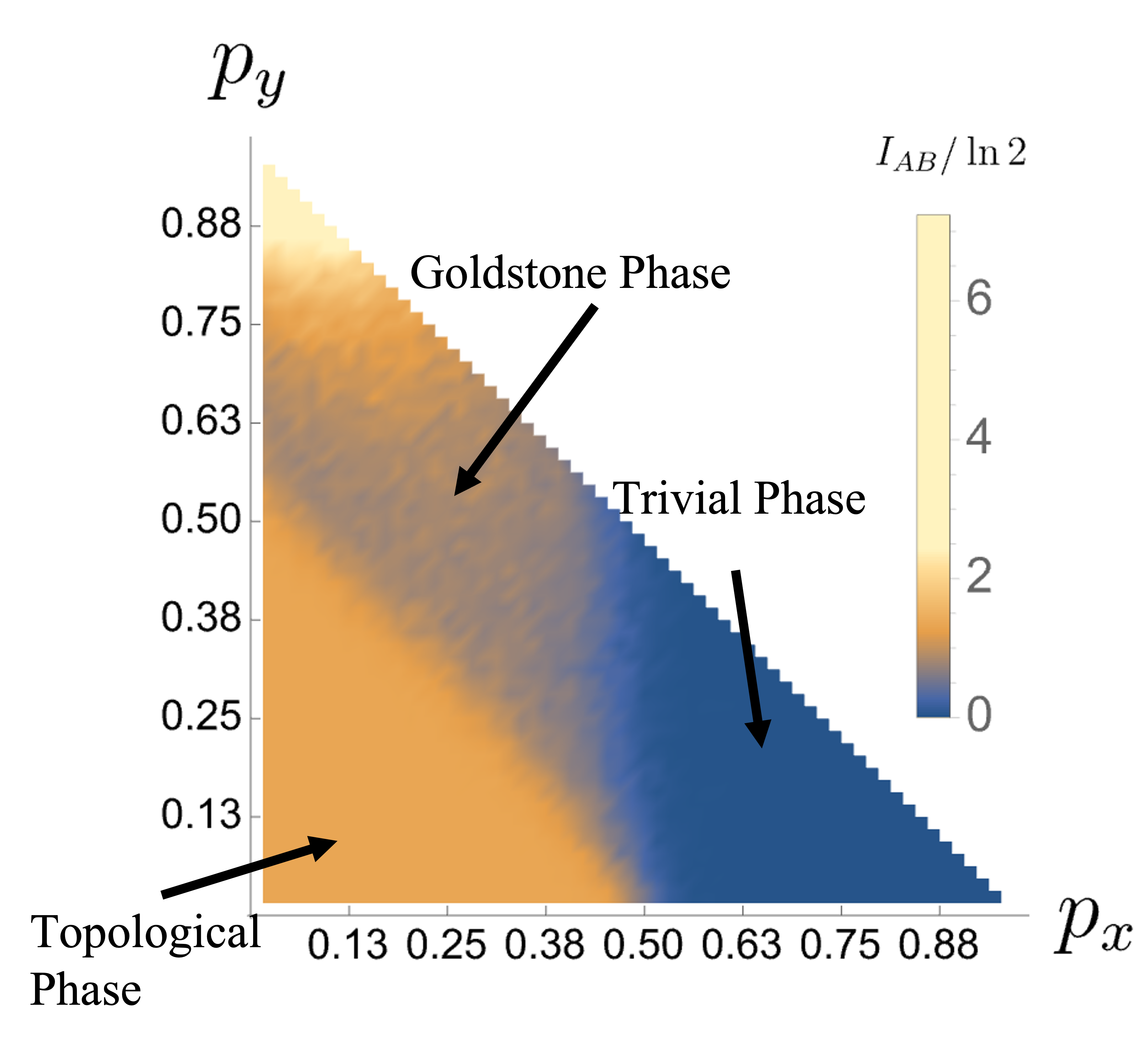
Figure 26: (Lieb lattice with X measurement on vertices) Mutual information $I_{AB}$ of antipodal domains $A$ and $B$, with $L_{A}=L_{B}=L/4$. Phases are marked by different colors, as $I_{AB}$ behaves differently in different phases.

V.2.3 Entanglement Transition in Square Lattice Cluster State

We now investigate the boundary state entanglement structure of the square lattice cluster state with random Pauli measurements in the bulk. We take the smooth boundary condition for the Square Lattice cluster state as shown in Fig. 8b. Consider random $X/Y/Z$ measurement with the measurement rate satisfying $p_{x}+p_{y}+p_{z}=1$. The phase diagram is shown in Fig. 27. When $X/Y$ measurement dominates, the boundary state is in the volume-law phase. When $Z$ measurement dominates, the boundary state is in the area-law phase.

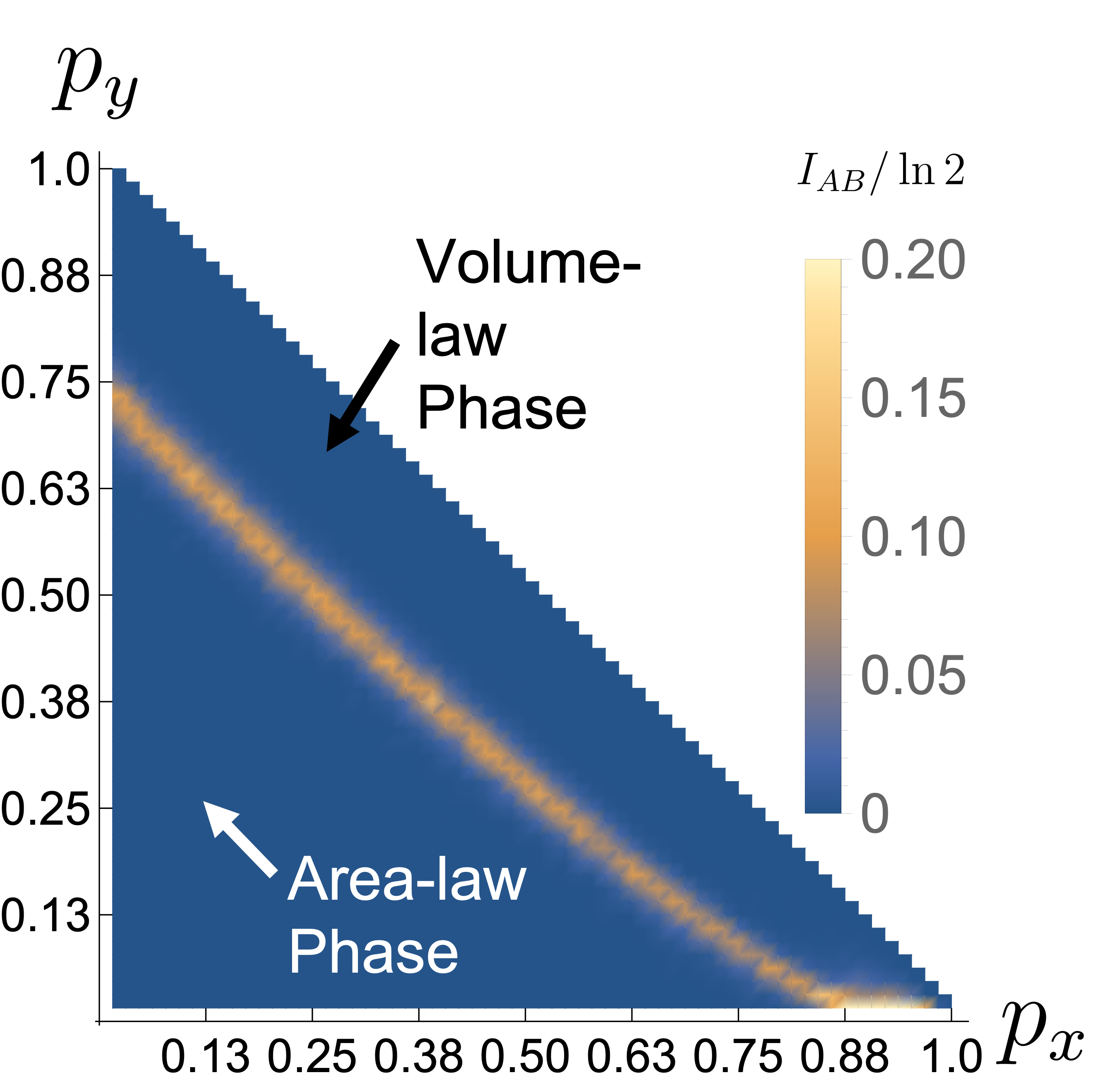
Figure 27: (Square lattice model) Mutual information $I_{AB}$ of antipodal domains $A$ and $B$, with $L_{A}=L_{B}=L/8$. The yellow line (mutual information peak) marks the phase boundary.

.

The volume-law to the area-law phase transition along $p_{y}=0$ is studied in our previous work Ref. [24]. Here, we investigate the boundary state entanglement transition along the line with $p_{x}=0$. The mutual information collapses to

$$I_{AB}\sim h(L^{1/\nu}(p_{y}-p_{y}^{c})),~{}\nu=1.3,$$ (158)

with data collapse shown in Fig. 28c. At the critical point $p_{y}=0.743$, the entanglement entropy, as shown in Fig. 28a is

$$S_{A}/\ln 2\sim 1.6\ln\sin(\frac{\pi L_{A}}{L})$$ (159)

and the mutual information is a function of the cross ratio and scales like

$$I_{AB}\sim\chi_{AB}^{2}$$ (160)

as shown in Fig. 28b.

We argue that the criticality observed along the $p_{x}=0$ line of the square lattice model and the Lieb lattice model falls within the same universality class as the volume-law to area-law entanglement transition in the 1+1D hybrid random Clifford circuit presented in [3]. Several reasons support this claim:

First, they exhibit the same critical exponents for entanglement entropy scaling, as illustrated in Figs. 22c and  28a

$$S_{A}\sim 1.6\ln\sin\left(\frac{\pi L_{A}}{L}\right).$$

Second, they both display the same critical mutual information scaling,

$$I_{AB}\sim\chi_{AB}^{2},$$

as shown in Figs. 23c and 28b. Additionally, their mutual information collapses to the same universal function with the same exponents $\nu=1.3$, as depicted in Fig. 29. These critical exponents agree with the ones extracted in [3].

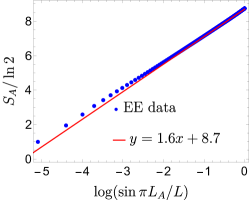
(a) Critical entanglement scaling, $p_{y}=0.743$, $p_{x}=0$

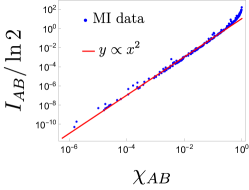
(b) Critical mutual information scaling, $p_{y}=0.743$, $p_{x}=0$

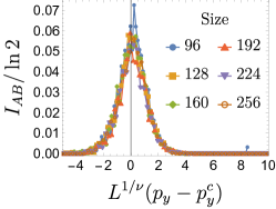
(c) Mutual information data collapse at $p_{y}^{c}=0.743$, $p_{x}=0$, $\nu=1.3$

Figure 28: Volume-law to area-law phase transition on the square lattice.

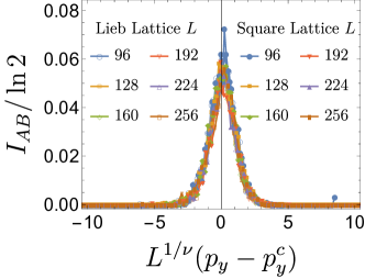
Figure 29: Mutual information data collapse for Lieb/Square lattice model along $p_{x}=0$ with $\nu=1.3$. Empty/Filled icons label the Lieb/Square lattice mutual information data.

In summary, our numerical observations demonstrate that cluster states defined on the Lieb lattice and square lattice exhibit entanglement phase transition on the 1D boundary induced by the bulk measurement. Such phase transition is closely related to the measurement-induced phase transition observed in the 1+1D hybrid circuits.[1, 2, 3, 4, 5, 6, 7, 8, 9, 10, 11, 12, 13, 14, 15, 16, 17]

VI Conclusion and Discussion

In this work, we have focused on the entanglement structure of the 1D boundary state and its relevance to the computational complexity of the cluster state sampling problem and the Ising partition function evaluation. We have established an equivalence between the sampling problem and the 2D Ising partition function, elucidating how this information can be encoded within the 1D boundary state. We have also explored dynamic boundary state generation and its connection to 1+1D non-unitary evolution. Finally, we numerically studied the boundary entanglement transitions induced by bulk measurements, specifically on the cluster states generated on the Lieb and square lattices. This method allowed us to pinpoint efficient regimes for evaluating the Ising partition function.

In Section II, we established a crucial connection between sampling the cluster state and evaluating the classical Ising partition function. This connection was unveiled by demonstrating that the inner product between the single qubit product state and the 2D cluster state follows the identical form as the classical Ising partition function with complex variables (as indicated in Eq. 22). As a result, the hardness of the cluster state sampling problem was found to be equivalent to the evaluation of the 2D Ising partition function.

In Sec. III, we illustrated that the 1D boundary state encodes all the information of the Ising partition function. A 1D wave function can be represented in a matrix product state, whose complexity is determined by its entanglement structure. This observation led us to a significant insight: the task of approximating the Ising partition function can be directly mapped to understanding the entanglement scaling of the 1D boundary state. When the boundary state exhibits a volume-law entanglement scaling, it signifies that the partition function is challenging to evaluate efficiently. Conversely, if the boundary state exhibits area-law entanglement scaling, it indicates that the corresponding Ising partition can be efficiently evaluated using classical computational resources.

In Sec. IV, we provided two dynamical approaches to generate the 1D boundary state. In the first approach, based on the transfer matrix, we explicitly established the correspondence between the single qubit measurement on the Lieb lattice cluster state and the non-unitary gates involved in 1+1D non-unitary dynamics. In the second approach, we employed a specific order of contractions of 2D tensor networks to obtain the boundary state, and demonstrated that such an order can be naturally interpreted as a 1+1D dynamics.

In Sec. V, we studied the boundary entanglement structure using two complementary numerical methods. First, we explicitly implemented the tensor network inspired dynamics to find that the boundary state undergoes an entanglement transition as the measurement direction $\hat{n}$ is varied. This transition is similar to the measurement-induced transition found in 1+1D non-unitary circuits. We found that the manifolds in which $\hat{n}$ ought to be varied to observe such a transition depended crucially on the geometry of the lattice. We related the presence of this transition, to the nature of the weights – positive, real or complex – in corresponding Ising-type partition functions and consequently, draw conclusions about the ease of their approximation. We also showed that randomness in the bulk measurement outcomes was crucial to the existence of volume-law phases in the boundary state. Secondly, we utilized the classical simulability of Pauli gates to study the behavior of the boundary states under random Pauli measurements. We found similar entanglement phase transitions here as well, supporting the generality of such transitions.

As emphasized throughout our work, our research offers a fresh perspective on computational complexity through boundary entanglement. Moreover, such an entanglement perspective can provide insight into measurement-based quantum computing systems (MBQCs), where the computation is done by controlling the measurement pattern on a resource state [42]. A crucial question arises in the realm of MBQCs: Is the resource state universal? Our study provides insights by demonstrating that the Lieb/Square lattice cluster state can prepare a boundary state with stable volume-law entanglement. This observation aligns with the assertion that Lieb/Square lattice cluster states can serve as universal resource states, as previously indicated [26, 43, 44]. In contrast, non-universal states, such as the toric code state, fail to generate boundary states with volume-law entanglement. This highlights how boundary entanglement analysis can be a valuable tool for determining whether the resource states are universal.

For further directions, we aim to extend this concept to other 2D resource states and explore whether similar approaches can yield interesting 1D boundary states. Additionally, we intend to investigate whether the computational power of thermal states can be characterized by the boundary entanglement structures.

Appendix A Bipartite Cluster State and Ising model

This appendix presents an alternative approach to establish the connection between sampling the bipartite cluster state and the Ising partition function, drawing on techniques introduced in [28].

The cluster state $\ket{\Psi}$ serves as a ground state of the following Hamiltonian:

$$H=-\frac{\Delta}{2}\sum_{i}K_{i}\quad\text{where}\quad K_{i}=X_{i}\prod_{n\in N_{i}}Z_{n}.$$ (161)

Here, $\Delta$ represents the energy gap, and $N_{i}$ denotes the neighboring sites of $i$ [56]. For cluster states defined on a bipartite graph, the Hamiltonian can be expressed as:

$$H=-\frac{\Delta}{2}\left(\sum_{i\in\circ}K_{i}+\sum_{j\in\bullet}K_{j}\right).$$ (162)

The ground state can be directly expressed using classical Ising spins $s$ defined on $\circ$ as follows:

$$\ket{\Psi}=\frac{1}{2^{|\circ|}}\sum_{s}\bigotimes_{i\in\circ,j\in\bullet}\ket{s_{i}}_{i}\otimes\ket{Q_{j}}_{j},$$ (163)

where $Z_{i}\ket{s_{i}}=s_{i}\ket{s_{i}}$, $X_{j}\ket{Q_{j}}=Q_{j}\ket{Q_{j}}$, and $Q_{j}=\prod_{i\in N_{j}}s_{i}$. It can be verified that for any $l\in\bullet$:

$$K_{l}\ket{\Psi}=\sum_{s}Q_{l}\times\prod_{n\in N_{l}}s_{n}\bigotimes_{i\in\circ,j\in\bullet}\ket{s_{i}}_{i}\otimes\ket{Q_{j}}_{j}$$ (164)

$$=\sum_{s}\bigotimes_{i\in\circ,j\in\bullet}\ket{s_{i}}_{i}\otimes\ket{Q_{j}}_{j},$$

as $Q_{l}\times\prod_{n\in N_{l}}s_{n}=1$ by definition. For any $m\in\circ$:

$$K_{m}\ket{s_{m}}_{m}\bigotimes_{n\in N_{m}}\ket{Q_{n}}_{n}=\ket{\overline{s_{m}}}_{m}\bigotimes_{n\in N_{m}}\ket{\overline{Q_{n}}}_{n},$$ (165)

which effectively flips the Ising spin $s_{m}\to\overline{s_{m}}$. We therefore have $K_{m}\ket{\Psi}=\ket{\Psi}$ for any $m\in\circ$. It is now evident that $\ket{\Psi}$ is the ground state of Eq. 161, hence the cluster state.

For simplicity, we parameterize the measurement wave function as:

$$\ket{\phi}_{i}= \sum_{s_{i}}\exp(h_{i}s_{i})\ket{s_{i}}_{i} \text{for }i\in\circ$$ (166)

$$\ket{\phi}_{j}= \sum_{Q_{j}}\exp(K_{j}Q_{j})\ket{Q_{j}}_{j} \text{for }j\in\bullet$$

with $h_{i},K_{j}\in\mathbb{C}$, and again $Z_{i}\ket{s_{i}}=s_{i}\ket{s_{i}}$, $X_{j}\ket{Q_{j}}=Q_{j}\ket{Q_{j}}$. The overlap function is then:

$$\bigotimes_{i\in\circ,j\in\bullet}\bra{\phi}_{i}\otimes\bra{\phi}_{j}\cdot\ket{\Psi}=\mathcal{Z}$$ (167)

where:

$$\mathcal{Z}=\sum_{s}\exp\left(\sum_{j\in\bullet}K_{j}Q_{j}+\sum_{i\in\circ}h_{i}s_{i}\right)$$ (168)

is the Ising partition function, taking $Q_{j}=\prod_{n\in N_{j}}s_{n}$. Thus, we recover Eq. 22.

Rewriting Eq. 166 in the $Z$ basis, we relate the Ising parameters $\{K,h\}$ with the weight parameters introduced in Eq. 4:

$$\exp(-2h_{i})= W_{i} \text{for }i\in\circ$$ (169)

$$\exp(-2K_{j})= \frac{1-W_{j}}{1+W_{j}} \text{for }j\in\bullet.$$

This relationship corresponds to Eq 24.

Appendix B Boundary Condition and Initial State

In this section, we discuss the relation between the shape of the Lieb lattice boundary and the initial state $\ket{\Psi}_{0}$ of the dynamics given by the Ising transfer matrix shown in Sec. IV. As previously shown in App. A. The cluster state defined on the lieb lattice is given by

$$\ket{\Psi}=\frac{1}{2^{|\circ|}}\sum_{s}\bigotimes_{i\in\circ,j\in\bullet}\ket{s_{i}}_{i}\otimes\ket{\prod_{n\in N_{j}}s_{n}}_{j},$$ (170)

where $\prod_{n\in N_{j}}s_{n}$ is the product over spins on the neighbouring sites of $j$. Taking into account the boundary of the lieb lattice, we modify the wave function to

$$\ket{\Psi}=\frac{1}{2^{|\circ|}}\sum_{s}\bigotimes_{i\in\circ,j\in\bullet}\ket{s_{i}}_{i}\otimes\ket{\prod_{n\in N_{j}}s_{n}}_{j}\otimes\ket{\psi[s_{k}]},$$ (171)

where $\ket{\psi[s_{k}]}$ labels the boundary condition and $s_{k}$ labels the boundary spin configuration.

For the “smooth” boundary condition, the boundary stabilizer is $g_{m}=X_{m}Z_{k}Z_{l}$ where $m=\langle k,l\rangle$ is the edge connecting vertices $k,l$ on the boundary and $g_{k}=X_{k}Z_{l}Z_{m}Z_{p}$ where $k$ is the vertex shared by edges $l,m,p$. $\ket{\psi_{0}[s_{k}]}$ is naturally

$$\ket{\psi_{0}[s_{k}]}=\bigotimes_{m\in\bullet,l\in\circ}\ket{s_{k}s_{l}}_{m}\ket{s_{k}}_{l}$$

which is physically the “free” boundary condition of the Ising model. The boundary term of the Ising partition function $\mathcal{Z}_{\text{b.t}}$ is given by overlap $\innerproduct{\phi}{\psi_{0}[s_{k}]}$

$$\mathcal{Z}_{\text{b.t}}=\sum_{s}\exp(\sum_{j}K_{j}s_{l}s_{m}+\sum_{k}h_{k}s_{k}),$$ (172)

which is the ”free” boundary condition of the Ising model. The initial state of the Ising transfer matrix dynamics is thus

$$\ket{\Psi_{0}}\equiv\frac{1}{2^{|\{s_{\partial\mathcal{M}}\}|}}\sum_{s_{\partial\mathcal{M}}}\ket{s_{\partial\mathcal{M}}}.$$

As for the “rough” boundary condition, the boundary stabilizer is $g_{m}=X_{m}Z_{k}$ where $m$ is the boundary edge connected to site $k$ and $g_{k}=X_{k}Z_{l}Z_{m}Z_{p}Z_{q}$ where $k$ is the vertex shared by edges $l,m,p,q$, and $m$ is the boundary edge. We may write the boundary term as

$$\ket{\psi_{0}[s_{k}]}=\bigotimes_{m}\ket{s_{k}}_{m}.$$ (173)

where $X_{m}\ket{s_{k}}_{m}=s_{k}\ket{s_{k}}_{m}$. The boundary term is

$$\mathcal{Z}_{\text{b.t}}=\sum_{s}\exp(\sum_{k}h_{k}^{\text{ext}}s_{k}),$$ (174)

since the boundary qubit is labeled by a single Ising spin. The single-site measurements on the boundary edge result in an external Ising magnetic field in the following form

$$\exp(-2h_{k}^{\text{ext}})=\frac{1-W_{m}}{1+W_{m}}.$$ (175)

where $W_{m}$ is the measurement weight $m$ on the boundary. In another perspective, we may regard such external field as bulk Ising spins couple to a fixed boundary spin $s_{k}=+1$ for all $k$ on the boundary, and the boundary term is written as

$$\mathcal{Z}_{\text{b.t}}=\sum_{s}\exp(\sum_{k}h_{k}^{\text{ext}}s_{k}s_{p});$$ (176)

$$s_{p}=1,~{}\forall p~{}\text{on boundary}.$$

The external magnetic field is now interpreted as Ising spins couple to a fixed boundary $s_{p}=1$ for all $p$ on the boundary

$$\ket{\psi_{0}[s_{p}]}=\bigotimes_{p}\ket{s_{p}=+1}_{p}$$ (177)

where $Z_{p}\ket{s_{k}=+1}_{p}=\ket{s_{p}=+1}_{p}$, and the fixed boundary condition results in the initial state

$$\ket{\Psi_{0}}=\ket{s_{\partial_{M}}=+1}.$$ (178)

Appendix C Overlap function as Ising gauge field

In this section, we demonstrate that the overlap function on the Lieb lattice can also be expressed using the $\mathbb{Z}_{2}$ gauge field partition function on a square lattice

$$\mathcal{Z}=\sum_{\tau}\exp\left(\sum_{p=\langle a,b\rangle^{\prime}}\tilde{h_{p}}\tau_{p}+\sum_{i}\tilde{K_{i}}\prod_{q\in\square_{i}}\tau_{q}\right),$$

and $X$ measurements with outcome $m_{i}$ on vertex $i$ correspond to applying a flux constraint on the gauge field

$$\prod_{q\in\square_{i}}\tau_{q}=m_{i}.$$

Directly taking $\tau=\sigma_{a}\sigma_{b}$, we recover the Ising partition function

$$\mathcal{Z}=\sum_{\sigma}\exp\left(\sum_{p=\langle a,b\rangle^{\prime}}\tilde{h_{p}}\sigma_{a}\sigma_{b}\right).$$

As illustrated in Fig. 30, the edges of the Lieb lattice are colored $\bullet$, and the vertices $\circ$. We assign each vertex $i$ a classical spin $s_{i}$, and each edge $p=\langle j,k\rangle$ a domain-wall variable $Q_{p=\langle j,k\rangle}=s_{j}s_{k}$ with $j,k$ being vertices connected by edge $p$. Plugging everything into Eq. 168, we recover Eq. 25:

$$\mathcal{Z}=\sum_{s}\exp\left(\sum_{p=\langle j,k\rangle}K_{p}s_{j}s_{k}+\sum_{i}h_{i}s_{i}\right),$$

which corresponds to a 2D classical Ising model with a magnetic field.

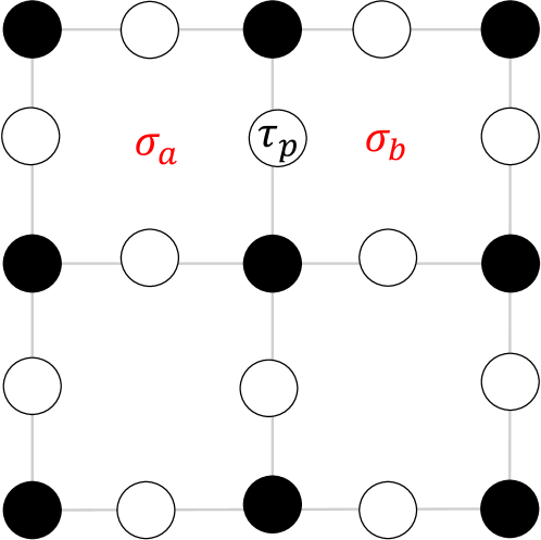
Figure 30: Alternative bipartition of the Lieb lattice. Physical $\mathbb{Z}_{2}$ degrees of freedom $\tau_{p}$ are defined on the edge $p$, and the corresponding $\mathbb{Z}_{2}$ transformations $\sigma_{a},\sigma_{b}$ are assigned to neighboring plaquettes $a$ and $b$.

Now, we reverse the color of the edges and vertices. The edges are colored $\circ$, and the vertices $\bullet$. We assign each edge $p=\langle a,b\rangle^{\prime}\in\circ$ a $\mathbb{Z}_{2}$ variable $\tau_{p}$, and each site $i$ a $Q_{i}=\prod_{q\in\square_{i}}\tau_{q}$, where $\square_{i}$ denotes edges enclosing site $i$. To clarify the physical meaning, we parameterize the measurement wave function in Eq. 166 as:

$$\ket{\phi}_{p}= \sum_{\tau_{p}}\exp(\tilde{h_{p}}\tau_{p})\ket{\tau_{p}}_{p} \text{for }p\in\circ$$ (179)

$$\ket{\phi}_{i}= \sum_{Q_{i}}\exp(\tilde{K_{i}}Q_{i})\ket{Q_{i}}_{i} \text{for }i\in\bullet$$

where $Z_{p}\ket{\tau_{p}}_{p}=\tau_{p}\ket{\tau_{p}}_{p}$ and $X_{i}\ket{Q_{i}}_{i}=Q_{i}\ket{Q_{i}}$. The overlap function becomes:

$$\mathcal{Z}=\sum_{\tau}\exp\left(\sum_{p=\langle a,b\rangle^{\prime}}\tilde{h_{p}}\tau_{p}+\sum_{i}\tilde{K_{i}}\prod_{q\in\square_{i}}\tau_{q}\right),$$ (180)

which gives the partition function for $\mathbb{Z}_{2}$ gauge theory, as $\mathcal{Z}$ remains invariant under the transformation of $\tau_{p}$:

$$\tau_{p}\to\tau_{p}\sigma_{a}\sigma_{b}\quad\text{where}\quad\sigma\in\mathbb{Z}_{2},$$ (181)

and $a,b$ label the plaquettes sharing edge $p$. The relationship between $\{\tilde{K},\tilde{h}\}$ and the weight parameters $\{W_{i}\}$ is given by:

$$\exp(-2\tilde{K}_{i}) =\frac{1-W_{i}}{1+W_{i}} \text{for }i\in\circ$$ (182)

$$\exp(-2\tilde{h_{p}}) =W_{p} \text{for }p\in\bullet.$$

When measuring the vertex sites along $X$, we have $\tilde{K}_{i}\to+\infty\times m_{i}$, where $m_{i}$ is the measurement outcome on vertex $i$. Consequently, we obtain:

$$\mathcal{Z}=\sum_{\tau}\exp\left(\sum_{p=\langle a,b\rangle^{\prime}}\tilde{h_{p}}\tau_{p}\right)\prod_{i}(1+m_{i}\prod_{q\in\square_{i}}\tau_{q}).$$ (183)

The second term $\prod_{i}(1+m_{i}\prod_{q\in\square_{i}}\tau_{q})$ can be understood as a constraint on $\tau$:

$$\prod_{q\in\square_{i}}\tau_{q}=m_{i}.$$ (184)

When all measurement outcomes are set to $+1$, we have $\prod_{q\in\square_{i}}\tau_{q}=1$ for all vertices $i$, implying that $\tau=\sigma_{a}\sigma_{b}$. Thus, the overlap function becomes:

$$\mathcal{Z}=\sum_{\sigma}\exp\left(\sum_{p=\langle a,b\rangle^{\prime}}\tilde{h_{p}}\sigma_{a}\sigma_{b}\right),$$ (185)

with $\exp(-2\tilde{h_{p}})=W_{p}$. This corresponds to a Kramers-Wannier dual of Eq. 25 at $h=0$.

References

- Li et al. [2018] Y. Li, X. Chen, and M. P. A. Fisher, Quantum zeno effect and the many-body entanglement transition, Phys. Rev. B 98, 205136 (2018).
- Chan et al. [2019] A. Chan, R. M. Nandkishore, M. Pretko, and G. Smith, Unitary-projective entanglement dynamics, Phys. Rev. B 99, 224307 (2019).
- Li et al. [2019a] Y. Li, X. Chen, and M. P. A. Fisher, Measurement-driven entanglement transition in hybrid quantum circuits, Phys. Rev. B 100, 134306 (2019a).
- Choi et al. [2020] S. Choi, Y. Bao, X.-L. Qi, and E. Altman, Quantum error correction in scrambling dynamics and measurement-induced phase transition, Phys. Rev. Lett. 125, 030505 (2020).
- Bao et al. [2020] Y. Bao, S. Choi, and E. Altman, Theory of the phase transition in random unitary circuits with measurements, Phys. Rev. B 101, 104301 (2020).
- Gullans and Huse [2020] M. J. Gullans and D. A. Huse, Dynamical purification phase transition induced by quantum measurements, Phys. Rev. X 10, 041020 (2020).
- Jian et al. [2020] C.-M. Jian, Y.-Z. You, R. Vasseur, and A. W. W. Ludwig, Measurement-induced criticality in random quantum circuits, Phys. Rev. B 101, 104302 (2020).
- Skinner et al. [2019] B. Skinner, J. Ruhman, and A. Nahum, Measurement-induced phase transitions in the dynamics of entanglement, Physical Review X 9, 031009 (2019).
- Li and Fisher [2021] Y. Li and M. P. A. Fisher, Statistical mechanics of quantum error correcting codes, Phys. Rev. B 103, 104306 (2021).
- Hoke et al. [2023] J. C. Hoke, M. Ippoliti, D. Abanin, R. Acharya, M. Ansmann, F. Arute, K. Arya, A. Asfaw, J. Atalaya, J. C. Bardin, A. Bengtsson, G. Bortoli, A. Bourassa, J. Bovaird, L. Brill, M. Broughton, B. B. Buckley, D. A. Buell, T. Burger, B. Burkett, N. Bushnell, Z. Chen, B. Chiaro, D. Chik, C. Chou, J. Cogan, R. Collins, P. Conner, W. Courtney, A. L. Crook, B. Curtin, A. G. Dau, D. M. Debroy, A. D. T. Barba, S. Demura, A. D. Paolo, I. K. Drozdov, A. Dunsworth, D. Eppens, C. Erickson, L. Faoro, E. Farhi, R. Fatem, V. S. Ferreira, L. F. Burgos, E. Forati, A. G. Fowler, B. Foxen, W. Giang, C. Gidney, D. Gilboa, M. Giustina, R. Gosula, J. A. Gross, S. Habegger, M. C. Hamilton, M. Hansen, M. P. Harrigan, S. D. Harrington, P. Heu, M. R. Hoffmann, S. Hong, T. Huang, A. Huff, W. J. Huggins, S. V. Isakov, J. Iveland, E. Jeffr, C. Jones, P. Juhas, D. Kafri, K. Kechedzhi, T. Khattar, M. Khezri, M. Kieferová, S. Kim, A. Kitaev, P. V. Klimov, A. R. Klots, A. N. Korotkov, F. Kostritsa, J. M. Kreikebaum, D. Landhuis, P. Laptev, K.-M. Lau, L. Laws, J. Lee, K. W. Lee, Y. D. Lensky, B. J. Lester, A. T. Lill, W. Liu, A. Locharla, F. D. Malone, O. Martin, J. R. McClean, T. McCourt, M. McEwen, K. C. Miao, A. Mieszala, S. Montazeri, A. Morvan, R. Movassagh, W. Mruczkiewicz, M. Neeley, C. Neill, A. Nersisyan, M. Newman, J. H. Ng, A. Nguyen, M. Nguyen, M. Y. Niu, T. E. O’Brien, S. Omonije, A. Opremcak, A. Petukhov, R. Potter, L. P. Pryadko, C. Quintana, C. Rocque, N. C. Rubin, N. S. D. Sank, K. Sankaragomathi, K. J. Satzinger, H. F. Schurkus, C. Schuster, M. J. Shearn, A. Shorter, N. Shutty, V. Shvarts, J. Skruzny, W. C. Smith, R. D. S. G. Sterling, D. Strain, M. Szalay, A. Torres, G. Vidal, B. Villalonga, C. V. Heidweiller, T. White, B. W. K. Woo, C. Xing, Z. J. Yao, P. Yeh, J. Yoo, G. Young, A. Zalcman, Y. Zhang, N. Zhu, N. Zobrist, H. Neven, R. Babbush, D. Bacon, S. Boixo, J. Hilton, E. Lucero, A. Megrant, J. Kelly, Y. Chen, V. Smelyanskiy, X. Mi, V. Khemani, and P. Roushan, Quantum information phases in space-time: measurement-induced entanglement and teleportation on a noisy quantum processor (2023), arXiv:2303.04792 [quant-ph] .
- Li et al. [2023] Y. Li, Y. Zou, P. Glorioso, E. Altman, and M. P. A. Fisher, Cross entropy benchmark for measurement-induced phase transitions, Phys. Rev. Lett. 130, 220404 (2023).
- Lavasani et al. [2021a] A. Lavasani, Y. Alavirad, and M. Barkeshli, Measurement-induced topological entanglement transitions in symmetric random quantum circuits, Nature Physics 17, 342 (2021a).
- Lavasani et al. [2022] A. Lavasani, Z.-X. Luo, and S. Vijay, Monitored quantum dynamics and the kitaev spin liquid (2022), arXiv:2207.02877 [cond-mat.str-el] .
- Lavasani et al. [2021b] A. Lavasani, Y. Alavirad, and M. Barkeshli, Topological order and criticality in monitored random quantum circuits, Phys. Rev. Lett. 127, 235701 (2021b).
- Sang and Hsieh [2021] S. Sang and T. H. Hsieh, Measurement-protected quantum phases, Phys. Rev. Res. 3, 023200 (2021).
- Ippoliti et al. [2021] M. Ippoliti, M. J. Gullans, S. Gopalakrishnan, D. A. Huse, and V. Khemani, Entanglement phase transitions in measurement-only dynamics, Phys. Rev. X 11, 011030 (2021).
- Sang et al. [2021] S. Sang, Y. Li, T. Zhou, X. Chen, T. H. Hsieh, and M. P. Fisher, Entanglement negativity at measurement-induced criticality, PRX Quantum 2, 030313 (2021).
- Sriram et al. [2023] A. Sriram, T. Rakovszky, V. Khemani, and M. Ippoliti, Topology, criticality, and dynamically generated qubits in a stochastic measurement-only kitaev model, Phys. Rev. B 108, 094304 (2023).
- Orús [2014] R. Orús, A practical introduction to tensor networks: Matrix product states and projected entangled pair states, Annals of Physics 349, 117 (2014).
- Arute et al. [2019] F. Arute, K. Arya, R. Babbush, D. Bacon, J. C. Bardin, R. Barends, R. Biswas, S. Boixo, F. G. Brandao, D. A. Buell, et al., Quantum supremacy using a programmable superconducting processor, Nature 574, 505 (2019).
- Terhal and DiVincenzo [2004] B. M. Terhal and D. P. DiVincenzo, Adaptive quantum computation, constant depth quantum circuits and arthur-merlin games (2004), arXiv:quant-ph/0205133 [quant-ph] .
- Bouland et al. [2019] A. Bouland, B. Fefferman, C. Nirkhe, and U. Vazirani, On the complexity and verification of quantum random circuit sampling, Nature Physics 15, 159 (2019).
- Napp et al. [2022] J. C. Napp, R. L. La Placa, A. M. Dalzell, F. G. S. L. Brandão, and A. W. Harrow, Efficient classical simulation of random shallow 2d quantum circuits, Phys. Rev. X 12, 021021 (2022).
- Liu et al. [2022] H. Liu, T. Zhou, and X. Chen, Measurement-induced entanglement transition in a two-dimensional shallow circuit, Phys. Rev. B 106, 144311 (2022).
- Bao et al. [2022] Y. Bao, M. Block, and E. Altman, Finite time teleportation phase transition in random quantum circuits (2022), arXiv:2110.06963 [quant-ph] .
- Bravyi and Raussendorf [2007] S. Bravyi and R. Raussendorf, Measurement-based quantum computation with the toric code states, Phys. Rev. A 76, 022304 (2007).
- Van den Nest et al. [2008] M. Van den Nest, W. Dür, and H. J. Briegel, Completeness of the classical 2d ising model and universal quantum computation, Phys. Rev. Lett. 100, 110501 (2008).
- De las Cuevas et al. [2009] G. De las Cuevas, W. Dür, M. Van den Nest, and H. J. Briegel, Completeness of classical spin models and universal quantum computation, Journal of Statistical Mechanics: Theory and Experiment 2009, P07001 (2009).
- Kitaev [2003] A. Kitaev, Fault-tolerant quantum computation by anyons, Annals of Physics 303, 2 (2003).
- Negari et al. [2023] A.-R. Negari, S. Sahu, and T. H. Hsieh, Measurement-induced phase transitions in the toric code (2023), arXiv:2307.02292 [quant-ph] .
- Bertini et al. [2019] B. Bertini, P. Kos, and T. c. v. Prosen, Exact correlation functions for dual-unitary lattice models in dimensions, Phys. Rev. Lett. 123, 210601 (2019).
- Ho and Choi [2022] W. W. Ho and S. Choi, Exact emergent quantum state designs from quantum chaotic dynamics, Phys. Rev. Lett. 128, 060601 (2022).
- Szyniszewski et al. [2019] M. Szyniszewski, A. Romito, and H. Schomerus, Entanglement transition from variable-strength weak measurements, Phys. Rev. B 100, 064204 (2019).
- Cirac et al. [2021] J. I. Cirac, D. Pérez-García, N. Schuch, and F. Verstraete, Matrix product states and projected entangled pair states: Concepts, symmetries, theorems, Rev. Mod. Phys. 93, 045003 (2021).
- Hauschild and Pollmann [2018] J. Hauschild and F. Pollmann, Efficient numerical simulations with Tensor Networks: Tensor Network Python (TeNPy), SciPost Phys. Lect. Notes , 5 (2018).
- Fishman et al. [2022a] M. Fishman, S. R. White, and E. M. Stoudenmire, The ITensor Software Library for Tensor Network Calculations, SciPost Phys. Codebases , 4 (2022a).
- Fishman et al. [2022b] M. Fishman, S. R. White, and E. M. Stoudenmire, Codebase release 0.3 for ITensor, SciPost Phys. Codebases , 4 (2022b).
- Guo et al. [2023] Y. Guo, J.-H. Zhang, Z. Bi, and S. Yang, Triggering boundary phase transitions through bulk measurements in 2d cluster states, arXiv preprint arXiv:2305.14231 (2023).
- Nahum et al. [2013] A. Nahum, P. Serna, A. M. Somoza, and M. Ortuñ o, Loop models with crossings, Physical Review B 87, 10.1103/physrevb.87.184204 (2013).
- Cardy [2001] J. Cardy, Conformal invariance and percolation (2001), arXiv:math-ph/0103018 [math-ph] .
- Barahona [1982] F. Barahona, On the computational complexity of ising spin glass models, Journal of Physics A: Mathematical and General 15, 3241 (1982).
- Raussendorf and Briegel [2001] R. Raussendorf and H. J. Briegel, A one-way quantum computer, Phys. Rev. Lett. 86, 5188 (2001).
- Raussendorf et al. [2019] R. Raussendorf, C. Okay, D.-S. Wang, D. T. Stephen, and H. P. Nautrup, Computationally universal phase of quantum matter, Phys. Rev. Lett. 122, 090501 (2019).
- Van den Nest et al. [2006] M. Van den Nest, A. Miyake, W. Dür, and H. J. Briegel, Universal resources for measurement-based quantum computation, Phys. Rev. Lett. 97, 150504 (2006).
- Li et al. [2019b] Y. Li, X. Chen, and M. P. Fisher, Measurement-driven entanglement transition in hybrid quantum circuits, Physical Review B 100, 134306 (2019b).
- Lee et al. [2022] J. Y. Lee, W. Ji, Z. Bi, and M. Fisher, Measurement-prepared quantum criticality: from ising model to gauge theory, and beyond, arXiv preprint arXiv:2208.11699 (2022).
- Bravyi et al. [2018] S. Bravyi, D. Gosset, and R. König, Quantum advantage with shallow circuits, Science 362, 308 (2018), https://www.science.org/doi/pdf/10.1126/science.aar3106 .
- Fujii and Morimae [2017] K. Fujii and T. Morimae, Commuting quantum circuits and complexity of ising partition functions, New Journal of Physics 19, 033003 (2017).
- Istrail [2000] S. Istrail, Statistical mechanics, three-dimensionality and np-completeness: I. universality of intracatability for the partition function of the ising model across non-planar surfaces (extended abstract), in Proceedings of the Thirty-Second Annual ACM Symposium on Theory of Computing, STOC ’00 (Association for Computing Machinery, New York, NY, USA, 2000) p. 87–96.
- Briegel and Raussendorf [2001] H. J. Briegel and R. Raussendorf, Persistent entanglement in arrays of interacting particles, Phys. Rev. Lett. 86, 910 (2001).
- Lund et al. [2017] A. P. Lund, M. J. Bremner, and T. C. Ralph, Quantum sampling problems, bosonsampling and quantum supremacy, npj Quantum Information 3, 15 (2017).
- Schuch et al. [2008] N. Schuch, M. M. Wolf, F. Verstraete, and J. I. Cirac, Entropy scaling and simulability by matrix product states, Phys. Rev. Lett. 100, 030504 (2008).
- Zhu et al. [2022] G.-Y. Zhu, N. Tantivasadakarn, A. Vishwanath, S. Trebst, and R. Verresen, Nishimori’s cat: stable long-range entanglement from finite-depth unitaries and weak measurements (2022), arXiv:2208.11136 [quant-ph] .
- Herringer and Raussendorf [2023] P. Herringer and R. Raussendorf, Classification of measurement-based quantum wire in stabilizer PEPS, Quantum 7, 1041 (2023).
- Cheng and Ippoliti [2023] Z. Cheng and M. Ippoliti, Efficient sampling of noisy shallow circuits via monitored unraveling (2023), arXiv:2306.16455 [quant-ph] .
- Raussendorf et al. [2005] R. Raussendorf, S. Bravyi, and J. Harrington, Long-range quantum entanglement in noisy cluster states, Phys. Rev. A 71, 062313 (2005).