Search for a new resonance decaying into two spin-0 bosons in a final state with two photons and two bottom quarks in proton-proton collisions at $\sqrt{s}=13\TeV$

Abstract

A search for a new boson X is presented using CERN LHC proton-proton collision data collected by the CMS experiment at $\sqrt{s}=13\TeV$ in 2016–2018, and corresponding to an integrated luminosity of 138. The resonance X decays into either a pair of Higgs bosons ${\PH\PH}$ of mass 125or an and a new spin-0 boson Y. One subsequently decays to a pair of photons, and the second or Y, to a pair of bottom quarks. The explored mass ranges of X are 260–1000and 300–1000, for decays to ${\PH\PH}$ and to ${\PH{\HepParticle{Y}{}{}}}$, respectively, with the Y mass range being 90–800. For a spin-0 X hypothesis, the 95% confidence level upper limit on the product of its production cross section and decay branching fraction is observed to be within 0.90–0.04fb, depending on the masses of X and Y. The largest deviation from the background-only hypothesis with a local (global) significance of 3.8 (2.8) standard deviations is observed for X and Y masses of 650 and 90, respectively. The limits are interpreted using several models of new physics.

0.1 Introduction

With the discovery of a Higgs boson in 2012 at the CERN LHC by the ATLAS and CMS Collaborations [HiggsdiscoveryAtlas, Chatrchyan:2012ufa, Chatrchyan:2013lba], the standard model (SM) has proven to describe most observed phenomena up to the scale [PhysRevLett.19.1264, SM2, SM3, Higgs:1964ia, Higgs:1964pj, CMS:2022dwd]. However, the important aspects of nature are left outside of this theory, such as dark matter and the nature of gravity. Beyond-SM (BSM) theories have been proposed to address these shortcomings, and many of these predict the existence of new massive spin-0 and -2 particles.

Among the BSMs, models with “warped extra dimensions” (WEDs) [Randall:1999vf, Randall:1999ee] postulate the existence of an additional spatial dimension in which the carriers of a quantized gravitational force (gravitons) propagate. In addition, according to the “Randall–Sundrum bulk model”, matter particles are also allowed to propagate in the extra dimension. This model contains massive resonances, the spin-0 radion [Goldberger:1999uk, Csaki:1999mp, Csaki:2000zn] and spin-2 bulk gravitons (excited modes of the gravitational field each separated by a characteristic mass scale) [Davoudiasl:1999jd, DeWolfe:1999cp, Agashe:2007zd], which have sizable branching fractions for decaying into ${\PH\PH}$ [Carvalho:2014lsg]. For this model, the fundamental scale is the reduced Planck scale $\overline{M_{pl}}$ with ultra-violate cutoff $\Lambda_{\text{R}}\equiv\sqrt{6}e^{-\kappa l}\overline{M_{pl}}$, where $\kappa$ and $l$ represent the curvature and the coordinate of the warped extra spatial dimension, respectively.

Supersymmetry (SUSY) is an extension of the SM which postulates a fermion-boson pairing symmetry (superpartners) [Golfand:1971iw, Wess:1974tw]. The minimal supersymmetric SM (MSSM) extends the SM Lagrangian by introducing an extra complex scalar doublet [Fayet:1974pd, Fayet:1977yc]. The next-to-minimal supersymmetric SM (NMSSM) [NMSSM2, NMSSM3] introduces one additional complex singlet field, and is the most straightforward supersymmetric extension to the SM where the electroweak scale originates from the SUSY-breaking scale. The NMSSM could provide a natural solution to the “unnaturalness” problem of MSSM [Kim:1983dt], wherein the difference between the $m_{\PH}$ and the Planck scale is of many orders of magnitude. In the NMSSM Higgs-sector, several spin-0 bosons exist, one of which can be associated with the discovered so far. More massive spin-0 bosons may decay to the lighter ones in this model.

Similar to the NMSSM, a model with two real scalar singlet fields (TRSM), in addition to the SM Higgs field, has been proposed [Robens:2019kga]. The mixing between the Higgs doublet and these additional scalar fields gives three massive scalar bosons, one of which can be identified as the SM-like . This model, too, allows the heavier scalar to decay into lighter scalars.

Motivated by the above BSM scenarios, this paper presents the search for a massive particle X decaying either to ${\PH\PH}$ or to and another spin-0 boson Y, using LHC proton-proton ($\Pp\Pp$) collision data collected by the CMS experiment in 2016–2018 at $\sqrt{s}=13\TeV$ and corresponding to a total integrated luminosity of 138. The results are interpreted within the framework of the BSMs presented above.

The search is performed in the final state with a pair of photons $\gamma$ and bottom $\PQb$ quarks ($\PGg\PGg\bbbar$). Figure 1 shows a tree-level Feynman diagram of the signal process. In using this channel, the ${\HepParticle{X}{}{}}\to{\PH\PH}$ search benefits from the combination of the $\PH\to\PGg\PGg$ decay, with its relatively large signal purity, and the $\PH\to\bbbar$ decay, with its large branching fraction. For the , the SM decay branching fractions [deFlorian:2016spz] are assumed. The ${\PH{\HepParticle{Y}{}{}}}$ search is independent of any assumption on ${\HepParticle{Y}{}{}}\to\bbbar$ branching fraction.

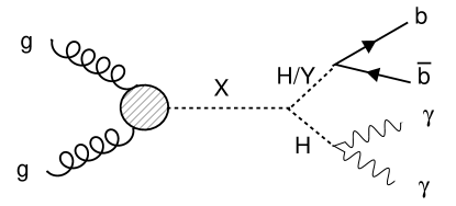
Figure 1: Feynman diagram showing a tree-level gluon-gluon fusion production of a BSM resonance X decaying to a pair of spin-0 bosons (${\PH\PH}$ or ${\PH{\HepParticle{Y}{}{}}}$), which then decay to the $\PGg\PGg\bbbar$ final state.

The analysis uses a strategy similar to the search for nonresonant production of ${\PH\PH}$ in the $\PGg\PGg\bbbar$ final state [Sirunyan:2018iwt, HIG-19-018_JHEP]. One candidate is reconstructed from a pair of photons $\PGg\PGg$, with their invariant mass $m_{\PGg\PGg}$ compatible with $m_{\PH}$. The candidate for the second boson, either or Y, is reconstructed from a pair of jets (particle jets originating from the fragmentation and hadronization of quarks), with their invariant mass $m_{\text{jj}}$ compatible with $m_{\PH}$ or with an assumed value of the Y boson mass $m_{{\HepParticle{Y}{}{}}}$. Events are selected using machine learning algorithms to suppress background contributions. The signal is extracted from a two-dimensional (2D) maximum likelihood fit spanning the ($m_{\PGg\PGg}$,$m_{\text{jj}}$) plane.

This paper is organized as follows: Section 0.2 provides a brief description of the CMS detector followed by the details of the data and simulated event samples in Section 0.3. The analysis strategy is discussed in Section 0.4, including background rejection methods along with the signal and background modeling studies. Section LABEL:sec:syst details the systematic uncertainties. The results are presented in Section LABEL:sec:res, and the analysis is summarized in Section LABEL:sec:sum. Tabulated results are provided in the HEPData record for this analysis [hepdata].

0.2 The CMS detector

The central feature of the CMS apparatus is a superconducting solenoid of 6m internal diameter, providing a magnetic field of 3.8T. Within the solenoid volume, there is a silicon pixel and strip tracker, a lead tungstate crystal electromagnetic calorimeter (ECAL), and a brass and scintillator hadron calorimeter (HCAL), each composed of a barrel and two endcap sections. Forward calorimeters extend the pseudorapidity $\eta$ coverage provided by the barrel and endcap detectors. Muons are measured in gas-ionization detectors embedded in the steel flux-return yoke outside the solenoid. A more detailed description of the CMS detector, together with a definition of the coordinate system used and the relevant kinematic variables, can be found in Ref. [CMSdetector].

Events of interest are selected using a two-tiered trigger system [Khachatryan:2016bia]. The first level (L1), composed of custom hardware processors, uses information from the calorimeters and muon detectors to select events at a rate of around 100kHz within a fixed latency of about 4 [CMS:2020cmk]. The second level, known as the high-level trigger, consists of a farm of processors running a version of the full event reconstruction software optimized for fast processing and reduces the event rate to around 1kHz before data storage [CMS_HLT].

The global event reconstruction, also called particle-flow (PF) event reconstruction [ParticleFlow], aims to reconstruct and identify each individual particle in an event (PF candidates), with an optimized combination of all subdetector information. In this process, the identification of the particle type (photon, electron, muon, charged or neutral hadron) plays an important role in the determination of the particle direction and energy.

Photons are identified as ECAL energy clusters not linked to the extrapolation of any charged particle trajectory to the ECAL. Electrons are identified as a primary charged particle track and potentially many ECAL energy clusters corresponding to this track extrapolation to the ECAL and to possible bremsstrahlung photons emitted along the way through the tracker material. Muons are identified as tracks in the central tracker consistent with either a track or several hits in the muon system, and associated with calorimeter deposits compatible with the muon hypothesis. Charged hadrons are identified as charged particle tracks neither identified as electrons, nor as muons. Finally, neutral hadrons are identified as HCAL energy clusters not linked to any charged hadron trajectory, or as a combined ECAL and HCAL energy excess with respect to the expected charged hadron energy deposit.

The energy of photons is obtained from the ECAL measurement. The raw ECAL energy is corrected in data using a multivariate analysis (MVA) based regression using Monte Carlo (MC) simulation of $\PZ\to\Pe\Pe$ events. In the simulated events, the energy of the photons is smeared to match the resolution in data [Sirunyan:2018ouh, cqr]. For photon identification, an MVA identification method (photon ID) based on photon shower shape, isolation, and kinematic variables is used [Sirunyan:2018ouh].

The energy of electrons is determined from a combination of the track momentum at the main interaction vertex, the corresponding ECAL cluster energy, and the energy sum of all bremsstrahlung photons attached to the track [CMS:2020uim]. The energy of muons is obtained from the corresponding track momentum. The energy of charged hadrons is determined from a combination of the track momentum and the corresponding ECAL and HCAL energies, corrected for the response function of the calorimeters to hadronic showers. Finally, the energy of neutral hadrons is obtained from the corresponding corrected ECAL and HCAL energies. In the barrel section of the ECAL, an energy resolution of about 1% is achieved for unconverted or late-converting photons in the tens of GeV energy range. The energy resolution of the remaining barrel photons is about 1.3% up to $\abs{\eta}=1$, changing to about 2.5% at $\abs{\eta}=1.4$. In the endcaps, the energy resolution is about 2.5% for unconverted or late-converting photons, and between 3 and 4% for the other ones [Khachatryan:2015iwa]. The $m_{\PGg\PGg}$ resolution, as measured in $\PH\to\PGg\PGg$ decays, is typically in the 1–2% range, depending on the measurement of the photon energies in the ECAL and the topology of the photons in the event [Sirunyan:2020xwk].

For each event, jets are clustered from these reconstructed particles using the infrared and collinear safe anti-algorithm [Cacciari:2008gp, Cacciari:2011ma] with a distance parameter of 0.4. Jet momentum is determined as the vectorial sum of all particle momenta in the jet, and is found from MC simulations to be, on average, within 5–10% of the true value over the whole transverse momentum spectrum and detector acceptance. Additional $\Pp\Pp$ interactions within the same or nearby bunch crossings (pileup) can contribute additional tracks and calorimetric energy depositions to the jet momentum. To mitigate this effect, charged particles identified to be originating from pileup vertices are discarded and an offset correction is applied for the remaining neutral particle contributions [Cacciari:2007fd]. Corrections, derived from MC simulations, are applied in order to bring the measured jet energies to that of the originating particles, average. Furthermore, in situ measurements of the momentum balance in dijet, $\PGg+$jet, $\PZ+$jet, and multijet events are used to account for any residual differences in the jet energy scale between data and MC simulations [Khachatryan:2016kdb]. An additional energy correction algorithm based on machine learning techniques is applied in this analysis to further improve the jet energy scale of jets [Sirunyan:2019wwa].

The jet energy resolution amounts typically to 15–20% at 30, 10% at 100, and 5% at 1 [Khachatryan:2016kdb]. Additional selection criteria are applied to each jet to remove jets potentially dominated by anomalous contributions from various subdetector components or reconstruction failures.

The missing transverse momentum vector is computed as the negative vector sum of all the PF candidates in an event, and its magnitude is denoted as  [METperformance]. The is modified to account for the corrections to the energy scale of the reconstructed jets in the event.

0.3 Data and simulated samples

The data used in this analysis were collected by the CMS detector from LHC $\Pp\Pp$ collisions at $\sqrt{s}=13\TeV$ in 2016–2018. The total analyzed data correspond to an integrated luminosity of 138 [Sirunyan:2759951, CMS-PAS-LUM-17-004, CMS-PAS-LUM-18-002]. Events are collected using the trigger conditions for the year 2016 (2017–2018) that requires two photons with thresholds $\pt^{\PGg_{1}}>30\GeV$ and $\pt^{\PGg_{2}}>18\ (22)\GeV$ and with $m_{\PGg\PGg}>90\GeV$, where $\PGg_{1}$ and $\PGg_{2}$ represent leading- and subleading-photons, respectively. The photons in the trigger algorithm have also to satisfy requirements on their calorimeter shower shapes, on the ratio of their energies deposited in the HCAL to that in the ECAL (identification variable), and on the carried by charged hadrons in the vicinity of the photon candidate (isolation requirement) [Sirunyan:2018ouh].

MC simulations of resonant production of X via gluon-gluon fusion (ggF), with subsequent decays, assuming a narrow-width approximation, to either ${\PH\PH}$ or ${\PH{\HepParticle{Y}{}{}}}$ were generated at next-to-leading order (NLO) using the package [Alwall:2014hca, NMSSM_UFO]. For the WED-motivated searches for spin-0 and -2 resonances, the package versions were 2.2.2 and 2.4.2, for the 2016 and 2017–2018 simulated samples, respectively. The signals were generated for $m_{{\HepParticle{X}{}{}}}$ in range 260–1000. For the NMSSM-motivated searches, the signal samples were generated using  2.6.5 for $300<m_{{\HepParticle{X}{}{}}}<1000\GeV$ and for $90<m_{{\HepParticle{Y}{}{}}}<800\GeV$. The samples were generated in steps of 100in $m_{{\HepParticle{X}{}{}}}$, and the kinematic mass distributions for intermediate $m_{{\HepParticle{X}{}{}}}$ were modeled by interpolating the shape parameters of the above simulated samples. Within signal simulations, a value of 125is considered for $m_{\PH}$.

The upper bound for $m_{{\HepParticle{X}{}{}}}$ search at 1is defined by the transition toward the Lorentz-boosted regime, where particles resulting from the hadronization of both quarks merge into a single jet. The upper range of $m_{{\HepParticle{Y}{}{}}}$ is set by the energy-momentum conservation rule for the on-shell particles $m_{{\HepParticle{Y}{}{}}}\leq m_{{\HepParticle{X}{}{}}}-m_{\PH}$. Below $m_{{\HepParticle{Y}{}{}}}=90\GeV$, the search capabilities are limited by the position of the kinematic turn-on in the $m_{\text{jj}}$ distribution.

The dominant backgrounds include the SM nonresonant multijet processes with up to two prompt photons, either as the irreducible $\PGg\PGg+$jets events or the reducible $\PGg+$jets events. The $\PGg\PGg+$jets background is modeled with  2.2.1 [Gleisberg:2008ta] at leading order (LO) and includes up to three additional partons at the matrix element level. The $\PGg+$jets background is modeled with  8.212 [Sjostrand:2014zea] at LO. The nonresonant background simulations are used only in the optimization and validation of the background estimation method using an MVA based discriminator.

Single productions, where the decays to $\PGg\PGg$, are considered as resonant backgrounds. These background events give a signal-like resonant distribution for $m_{\PGg\PGg}$, which is one of the observables in the analysis. The $\Pg\Pg\mathrm{F}\ \PH$ is simulated at NLO using  2.0 [Nason:2004rx, POWHEG_Frixione:2007vw, Alioli:2010xd, Bagnaschi:2011tu]. The vector-boson fusion production ($\mathrm{VBF}\ \PH$) and production in association with top quark pairs ($\ttbar\PH$) are simulated at NLO using  v2.2.2 (2016) or v2.4.2 (2017–2018). The production in association with a vector boson ($\PV\PH$) and in association with $\PQb$ quarks ($\bbbar\PH$) [Wiesemann_2015] are simulated using  v2.6.1. The cross sections and decay branching fractions are taken from Ref. [deFlorian:2016spz].

The simulated samples are interfaced with for parton showering and fragmentation with the standard -ordered parton shower scheme. The underlying event is modeled with , using the CUETP8M1 (CP5) tunes for 2016 (2017–2018) [Khachatryan:2015pea, Sirunyan:2019dfx]. Parton distribution functions (PDFs) are taken from the NNPDF3.0 [Ball:2014uwa] NLO (2016) or NNPDF3.1 [Ball:2017] next-to-NLO (2017–2018) except for the LO simulations, for which the PDF4LHC15_NLO_MC set at NLO [Carrazza:2015hva, Butterworth:2015oua, Dulat:2015mca, Harland-Lang:2014zoa, Ball:2014uwa] is used. The detector response is modeled using the  [Agostinelli:2002hh] toolkit. The simulated event samples also include a similar pileup as observed in the data, with an average of 23 (32) $\Pp\Pp$ interactions per bunch crossing in 2016 (2017–2018) data.

0.4 Analysis strategy

0.4.1 Object reconstruction and event preselections

Photons are considered if they are contained within the ECAL and tracker fiducial region of $\abs{\eta}<2.5$, excluding the ECAL barrel-endcap transition region ($1.44<\abs{\eta}<1.57$), and they should also pass the selections $\pt^{\PGg_{1}}/m_{\PGg\PGg}>1/3$, $\pt^{\PGg_{2}}/m_{\PGg\PGg}>1/4$, and $100<m_{\PGg\PGg}<180\GeV$. The primary $\Pp\Pp$ vertex associated with the diphoton system is identified using an MVA technique [Khachatryan:2014ira]. The efficiency of the correct vertex assignment is 99.9%, aided by the requirement of at least two jets in the $\PGg\PGg\bbbar$ final state.

Only events with at least two jets originating from the same vertex as the photon pairs are considered for the following selections. First, the jets are required to be within the tracker fiducial volume, so that track information can be used to identify heavy flavor (and ) jets. These jets should have $\pt>25\GeV$ and $\abs{\eta}<2.4$ ($<2.5$) for 2016 (2017–2018), while also passing jet identification criteria, in order to reject spurious jets from calorimeter noise [PUJID]. The $\abs{\eta}$ selection of jets is looser for the 2017–2018 data-taking years because of the installation of the new pixel detector at the beginning of 2017 [Vormwald_2019]. Then, the jets and photons are required to be separated by $\Delta{R}\equiv\sqrt{(\Delta\eta)^{2}+(\Delta\phi)^{2}}>0.4$, where $\Delta\eta$ and $\Delta\phi$ are the pseudorapidity and the azimuthal angle (measured in radians) differences between a photon and the closest jet, respectively. This selection is used in order to avoid counting of photons as jets. Finally, jet pairs with $70<m_{\text{jj}}<190$ (1200)for ${\PH\PH}$ (${\PH{\HepParticle{Y}{}{}}}$) analysis are retained for further selection, respectively.

For the identification of jets, a deep neural network (DNN) score-based tagger DeepJet [Sirunyan:2017ezt, Bols:2020bkb, CMS-DP-2018-058] is used. It utilizes information related to tracks and secondary vertex of jets. The pair with the highest sum of DeepJet discriminant scores in the event is selected as a (Y) candidate. In case no such pair is present the event is rejected. The physics object reconstruction and event preselection criteria are summarized in Table 0.4.1.

The ${\HepParticle{X}{}{}}$ candidate is reconstructed from the selected pairs of photons and jets. Figure 2 shows the $m_{\PGg\PGg}$, $m_{\text{jj}}$, and 4-body invariant mass $m_{\PGg\PGg\text{jj}}$ distributions in the data and MC simulations after the full set of selection criteria. The best estimate of the mass of the X candidate is given by the variable $\widetilde{M}_{\mathrm{X}}$, which has a better resolution than $m_{\PGg\PGg\text{jj}}$ [Kumar:2014bca] because of the resolution subtraction of $m_{\PGg\PGg}$ and $m_{\text{jj}}$, defined as:

$$\widetilde{M}_{\mathrm{X}}\equiv m_{\PGg\PGg\text{jj}}-(m_{\PGg\PGg}-m_{\PH})-(m_{\text{jj}}-{\rm m}_{\PH{~{}\rm or~{}}{\HepParticle{Y}{}{}}})$$ (1)

The improvement in resolution by using $\widetilde{M}_{\mathrm{X}}$ instead of $m_{\PGg\PGg\text{jj}}$ ranges from 30% at high $m_{{\HepParticle{X}{}{}}}$ up to 90% at low $m_{{\HepParticle{X}{}{}}}$.

Event preselection criteria. Photons Jets Variable Requirement Variable Requirement Leading photon $>m_{\PGg\PGg}/3$ $\pt$ $>25\GeV$ Subleading photon $>m_{\PGg\PGg}/4$ $\Delta R_{\PGg\text{j}}$ $>0.4$ $\abs{\eta}$ $<2.5$ $\abs{\eta}$ $<2.4~{}(2.5)$ for 2016 (2017–2018) Number of jets $>1$ $m_{\PGg\PGg}$ 100–180 $m_{\text{jj}}$ 70–190 (70–1200)for ${\PH\PH}$ (${\PH{\HepParticle{Y}{}{}}}$) Jet-pairs with the highest DeepJet score sum

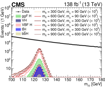
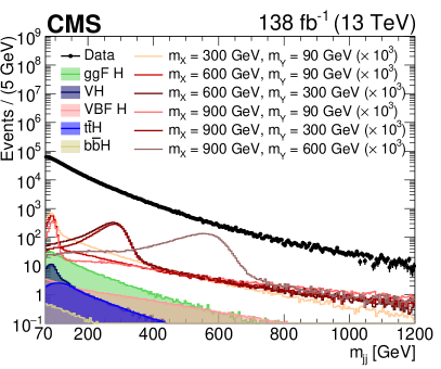
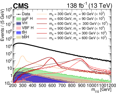
Figure 2: The $m_{\PGg\PGg}$ (upper left), $m_{\text{jj}}$ (upper right) and $m_{\PGg\PGg\text{jj}}$ (lower) distributions in data and MC simulations. The $m_{\text{jj}}$ distribution starts at 70. The signal distributions, shown for different values of $m_{{\HepParticle{X}{}{}}}$ and $m_{{\HepParticle{Y}{}{}}}$ with an assumption of 1fb cross section, have been scaled by a factor of $10^{3}$.

0.4.2 Nonresonant background separation

The dominant nonresonant backgrounds stem from the SM multijet processes with up to two prompt photons. A boosted decision tree (BDT) discriminant is trained using MC simulations to separate signal and nonresonant backgrounds $\PGg\PGg+$jets and $\PGg+$jets. For this purpose, a gradient boosting algorithm, XGBoost [xgboost] is used to develop a multiclass BDT classifier.

Various resonant $m_{{\HepParticle{X}{}{}}}$ and $m_{{\HepParticle{Y}{}{}}}$ hypotheses with different kinematic distributions are studied within the analysis. The phase space is subdivided into three regions for $m_{{\HepParticle{X}{}{}}}$ ($<500$, 500–700, and $>700\GeV$) and for $m_{{\HepParticle{Y}{}{}}}$ ($<300$, 300–500, and $>500\GeV$). These ranges are combined into nine $m_{{\HepParticle{X}{}{}}}$–$m_{{\HepParticle{Y}{}{}}}$ domains, three of which are forbidden by the energy conservation constraint $m_{{\HepParticle{Y}{}{}}}<m_{{\HepParticle{X}{}{}}}-m_{\PH}$. The mass ranges are decided according to the kinematic properties and Lorentz-boost factor, estimated by the quantity $m_{{\HepParticle{X}{}{}}}/(m_{\PH}+m_{{\HepParticle{Y}{}{}}})$ [Gouzevitch:2013qca], which defines similar angular properties. One BDT is trained per $m_{{\HepParticle{X}{}{}}}$–$m_{{\HepParticle{Y}{}{}}}$ region. For each mass range in $m_{{\HepParticle{Y}{}{}}}$ a dedicated $m_{\text{jj}}$ interval is defined: 70–400, 150–560, and 300–1000, respectively. Each interval is optimized to maximize the signal acceptance while leaving sufficient side bands in the mass distributions with a negligible signal contribution for background estimation.

All simulated ${\HepParticle{X}{}{}}\to{\PH{\HepParticle{Y}{}{}}}$ signal events that fit into a domain are combined into one sample with equal weights to build the signal sample. The simulated nonresonant background events are used as background samples, weighted by the products of their cross sections and the integrated luminosity. Before the training, the signal and background samples are normalized to unity. For ${\PH\PH}$ searches, the training with $m_{\text{jj}}$ interval 70–400is used since it already covers the $m_{\text{jj}}$ interval of 70–190.

The events are randomized and divided into train and test sets for every training. The input hyperparameters of the training are optimized using the 5-fold cross-validation [Hastie] to mitigate over-training. An early-stopping feature of XGBoost is also used to control the over-training. The BDT is trained for the three data-taking years together using three groups of input variables. The training strategy is validated by comparing the per year performance from the merged training with the performance obtained by the separate training for each year. The three types of BDT training input variables, based on the two photons and two jets associated with the X decay, are motivated by Ref. [HIG-19-018_JHEP]. They are:

1. Discriminating kinematic variables:

   • Helicity angles ($|\cos{\theta^{\rm CS}_{\rm HY}}|$, $\abs{\cos{\theta_{\text{jj}}}}$, $\abs{\cos{\theta_{\PGg\PGg}}}$), here CS refers to the Collins-Soper frame [PhysRevD.16.2219].

   • Minimum angular distances between photons and jets ($\Delta R_{\PGg\text{j}}$).

   • $\pt(\text{jj})/m_{\PGg\PGg\text{jj}}$ and $\pt(\PGg\PGg)/m_{\PGg\PGg\text{jj}}$.

   • $\pt(\PGg)/m_{\PGg\PGg}$ and $\pt(\text{j})/m_{\text{jj}}$ for leading and subleading photons and jets, respectively.

2. Object identification variables:

   • Leading- and subleading-photon ID to reject misidentified photon contribution

   • Leading- and subleading-jet b tagging discriminant to reject light jets

3. Resolution estimators:

   • Leading- and subleading-photons: Energy resolution ($\sigma_{\text{E}}$/E) and mass resolution ($\sigma_{m_{\PGg\PGg}}/m_{\PGg\PGg}$);

   • Leading- and subleading-jets: resolution ($\sigma_{\pt(\text{j})}/\pt(\text{j})$) and mass resolution ($\sigma_{m_{\text{jj}}}/m_{\text{jj}}$).

In addition to this, the transverse momentum deposits per unit area of the $\eta$–$\phi$ plane coming from pileup of the event, also known as the pileup transverse momentum density, is added in the inputs of the training to include pileup information which is different in the data-taking periods 2016–2018. The final BDT training output discriminates the signal from the background events by populating the signal events towards the high BDT score and background events towards the low BDT score. To preserve the numerical precision in defining optimal signal-enriched regions, the BDT outputs are transformed such that the signal distribution becomes uniform. The distribution of one of the BDT outputs for data and simulated events is shown in Fig. 3.

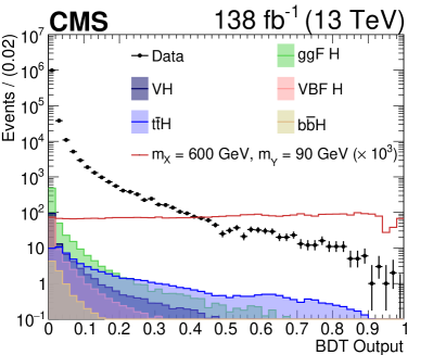
Figure 3: The distribution of BDT output in data and MC simulations for a signal in $m_{{\HepParticle{X}{}{}}}$ = 500–700and $m_{{\HepParticle{Y}{}{}}}<300\GeV$ range. The signal distribution, with an assumption of 1fb cross section, has been scaled by a factor of $10^{3}$.

0.4.3 Event classification

We classify events into three categories based on BDT output along with a selection on $\widetilde{M}_{\mathrm{X}}$. The optimization of the BDT categories and $\widetilde{M}_{\mathrm{X}}$ selection is performed independently aiming for the best signal sensitivity. The $\widetilde{M}_{\mathrm{X}}$ selection differs depending upon $m_{{\HepParticle{X}{}{}}}$, while the categorization remains the same for the signals within an $m_{{\HepParticle{X}{}{}}}$–$m_{{\HepParticle{Y}{}{}}}$ domain. The $\PGg\PGg\bbbar$ channel suffers from low data statistics due to the low selection efficiency and high purity. Therefore, a constraint on background statistics is also applied during the optimization of BDT categories to ensure enough background events to have robust background modeling.

For the ${\PH\PH}$ analysis, a selection containing at least 60% of the signal is defined on $\widetilde{M}_{\mathrm{X}}$ for each $m_{{\HepParticle{X}{}{}}}$ hypothesis as shown in Fig. 4. This selection remains the same for ${\PH\PH}$ and ${\PH{\HepParticle{Y}{}{}}}$ signals because, for low $m_{{\HepParticle{Y}{}{}}}$, the $\widetilde{M}_{\mathrm{X}}$-resolution of ${\PH{\HepParticle{Y}{}{}}}$ signals is similar to ${\PH\PH}$ signals. In contrast, for high $m_{{\HepParticle{Y}{}{}}}$, $\widetilde{M}_{\mathrm{X}}$ holds better resolution, giving higher signal efficiency with the same selection.

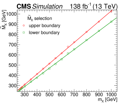
Figure 4: $\widetilde{M}_{\mathrm{X}}$ selection for each $m_{{\HepParticle{X}{}{}}}$ in ${\PH\PH}$ and ${\PH{\HepParticle{Y}{}{}}}$ signals. The red and green lines represent the upper and lower boundary of this selection.

We use signal and nonresonant background simulations to define categories based on the Punzi figure of merit [Punzi] defined as $\epsilon_{s}/(1+\sqrt{B})$, where $\epsilon_{s}$ is signal efficiency and $B$ refers to background yields. The category optimization remains independent of assuming any signal cross section since the figure of merit only uses signal efficiency, which prevents categorization bias towards any specific signal hypothesis. The categories for different $m_{{\HepParticle{X}{}{}}}$–$m_{{\HepParticle{Y}{}{}}}$ domains are provided in Table 0.4.3. The categories are labeled with 0 to 2 from the highest to lowest purity. For ${\PH\PH}$ searches, categorization in $m_{{\HepParticle{Y}{}{}}}$ < 300region is used.

The BDT based event classification according to defined $m_{{\HepParticle{X}{}{}}}$ (and $m_{{\HepParticle{Y}{}{}}}$) ranges for ${\PH\PH}$ (and ${\PH{\HepParticle{Y}{}{}}}$) searches. For ${\PH\PH}$ searches, the column with $m_{{\HepParticle{Y}{}{}}}$ < 300is used. The number represents the BDT scores showing a decreasing signal purity region from category 0 to 2. $m_{{\HepParticle{Y}{}{}}}$ < 300 $m_{{\HepParticle{Y}{}{}}}$ = [300–500] $m_{{\HepParticle{Y}{}{}}}$ > 500 $m_{{\HepParticle{X}{}{}}}$ < 500 $m_{{\HepParticle{X}{}{}}}$ = [500–700] $m_{{\HepParticle{X}{}{}}}$ > 700 CAT 0 = 0.63–1.0 CAT 1 = 0.33–0.63 CAT 2 = 0.17–0.33 CAT 0 = 0.55–1.0 CAT 1 = 0.40–0.55 CAT 2 = 0.21–0.40 CAT 0 = 0.50–1.0 CAT 1 = 0.30–0.50 CAT 2 = 0.21–0.30 CAT 0 = 0.60–1.0 CAT 1 = 0.35–0.60 CAT 2 = 0.18–0.35 CAT 0 = 0.35–1.0 CAT 1 = 0.24–0.35 CAT 2 = 0.18–0.24 CAT 0 = 0.40–1.0 CAT 1 = 0.29–0.40 CAT 2 = 0.13–0.29