Supplementary Material for:
Stability and Dynamics of Atom-Molecule Superfluids Near a Narrow Feshbach Resonance

I Preparation and Detection of Atomic and Molecular BECs

Figure S1: Molecule number and molecular BEC fraction prepared at different temperatures. a, Number of molecules created by associating atoms in ultracold atomic gases at different temperatures. The black (purple) data points are from 16.7 ms focused time-of-flight (ToF) (in-situ) measurement. Lower detection efficiency in the ToF measurement is due to inelastic molecular collision-induced loss during the additional time of flight compared to the in-situ imaging. b, Molecular BEC fraction measured from the focused ToF imaging of the molecular density $n_{m}$, which shows bimodal distribution at sufficiently low temperature. The inset is an example image of molecular density at 27 nK.

The procedure to prepare a Cs BEC in the lowest hyperfine ground state at 19.5 G for the quench experiments shown in Fig. 3(a-b) is the same as that in Ref. Zhang et al. (2023). The atomic BECs have 23,000 atoms with a BEC fraction of 80%. We detect the remaining atoms after the quench dynamics by absorption imaging the atoms back at the off-resonant field value 19.5 G. We detect the created molecules by first blowing away the remaining atoms using the atom imaging light pulse, dissociating molecules above the Feshbach resonance, and then releasing the atoms from dissociation into an isotropic harmonic trap for a quarter trap period before absorption imaging them Zhang et al. (2021, 2023). We normalize both the atomic and molecular population by the initial total atom number during the quench dynamics as shown in Fig. 3(a-b). The missing fraction is due to various loss processes. We extract the asymptotic molecular fraction in the quasi-steady state, as presented in Fig. 4(b), by averaging data in the time window between 1 ms and 3 ms in the dynamics.

To create pure molecular samples used for the experiments shown in Fig. 3(c), we first make evaporatively cooled ultracold atomic gases at 20.22 G. Then we switch to 19.89 G and ramp through the narrow g-wave Feshbach resonance to 19.83 G in 1.5 ms to associate atoms into molecules. After that, we quench the magnetic field to 19.5 G and apply a resonant light pulse to blow away the residual atoms. The resulting molecular temperature and population are characterized and shown in Fig. S1a, where fewer and colder molecules are created from initial atomic gases at lower temperature and population. When the temperature is low enough, the molecular density after the focused time-of-flight starts to develop bimodal distribution, from which we do fitting to extract the molecular BEC fraction (see Fig. S1b). We choose to use molecular BECs at 27 nK with a BEC fraction of 23(1)% as the initial condition for the experiments shown in Fig. 3(c). After the magnetic field quench, the atoms from molecule dissociation are imaged in-situ for higher detection efficiency.

II Quantifying the Resonance Width

Early experiments on a bosonic Feshbach resonance by Donley et. al.  Donley et al. (2002); Claussen et al. (2002) have focused on coherent oscillations between different Bose condensates below but near resonance. However, the Feshbach resonance employed, that of ⁸⁵Rb atoms at magnetic field $B_{0}=154.9$G, is very wide.

Using the many-body classification of resonance width in Ref. Ho et al. (2012) (see Scheme (B) in their Eq. (4)), we estimate the dimensionless resonance-width parameter to be $x=(k_{n}r_{*})^{-1}\sim 10^{3}\gg 1$ for ⁸⁵Rb. For details, see Table S1. Here, $k_{n}=(6\pi^{2}n)^{1/3}$ with $n$ the total atomic number density, and $r_{*}$ is a length scale defined from the experimental resonance width. As a consequence of the extremely large $x$, the closed channel molecular fraction near unitarity in these wide resonances is negligible Kokkelmans and Holland (2002). And the observed coherent oscillations in Refs. Donley et al. (2002); Claussen et al. (2002) are best interpreted as that between atomic and “molecular”-bound states, the latter of which are made up of open-channel atoms Köhler et al. (2003); Kokkelmans and Holland (2002); de las Heras et al. (2019); Corson and Bohn (2015) and should be contrasted with the actual closed-channel molecules.

In contrast, the ¹³³Cs g-wave resonance used in Refs. Zhang et al. (2021, 2023) is extremely narrow. A simple estimate shows that $x\sim 0.1\ll 1$, in agreement with the significant fraction of closed-channel molecules observed near unitarity in the experiments. The successful observation of molecules in this resonance not only enables us to explicitly study dissociation of molecular superfluids, but also provides us an opportunity to explore the role of the molecular superfluid component in post-quench dynamics starting with an initial state of open channel (atomic) superfluid condensate. Theoretically, the inherent narrowness of the resonance requires us to consider a fully two-channel formulation, in order to treat the dynamics adequately.

II.1 Experimental Feshbach-resonance parameters

In Table S1 we present the relevant experimental parameters that we have used to estimate the resonance width for ¹³³Cs, ⁸⁵Rb, and ³⁹K.

Table S1: Experimental parameters for Feshbach resonances in different Bose gases. In this table, $m_{1}$ is the atomic mass, $B_{0}$ is the experimental resonance point, $\Delta\mu_{m}$ is the magnetic moment difference between a pair of atoms in the open channel and a molecule in the closed channel, $\Delta B$ is the resonance-width in magnetic field, $a_{\mathrm{bg}}$ is the atom-atom background scattering length, and $n$ is the experimental number density of atoms. In the last column, $x\equiv(k_{n}r_{*})^{-1}=|k_{n}a_{\mathrm{bg}}|^{-1}|\Delta\mu_{m}\Delta B|/E_{\mathrm{bg}}$ is the dimensionless resonance-width parameter introduced in Ref. Ho et al. (2012). Here, $k_{n}=(6\pi^{2}n)^{1/3}$ and $E_{\mathrm{bg}}\equiv\hbar^{2}/(m_{1}a_{\mathrm{bg}}^{2})$. The data for ¹³³Cs, ⁸⁵Rb, and ³⁹K are collected from Refs. Zhang et al. (2021, 2023), Refs. Donley et al. (2002); Holland et al. (2001), and Refs. Eigen et al. (2018); D’Errico et al. (2007), respectively. $a_{B}$ is the Bohr radius, and $\mu_{B}$ is the Bohr magneton.

Atom	$m_{1}$	$B_{0}$	$\Delta\mu_{m}$	$\Delta B$	$a_{\mathrm{bg}}$	$n$	$x=(k_{n}r_{*})^{-1}$
133Cs	133 a. u.	19.849 G	0.57 $\mu_{B}$	8.3 mG	163 $a_{B}$	$2.9\times 10^{13}$ cm-3	$10^{-1}$
85Rb	84.9 a. u.	155 G	$-2.23$ $\mu_{B}$	11.06 G	$-450$ $a_{B}$	$3.9\times 10^{12}$ cm-3	$10^{3}$
39K	38.96 a. u.	402.7 G	1.5 $\mu_{B}$	52 G	$-29$ $a_{B}$	$5.1\times 10^{12}$ cm-3	$10^{2}$

III Derivation of Eq. (2) in the Main Text

In this section, we give detailed derivations of Eq. (2) in the main text. We start with the time-dependent trial wavefunction Corson and Bohn (2015),

$$|\Psi_{\mathrm{var}}(t)\rangle =\frac{1}{\mathcal{N}(t)}e^{\sum_{\sigma}\Psi_{\sigma 0}(t)\sqrt{V}a^{\dagger}_{\sigma\mathbf{k}=0}+\sum_{\mathbf{k}\neq 0,\sigma}^{\prime}\chi_{\sigma\mathbf{k}}(t)\;a^{\dagger}_{\sigma\mathbf{k}}a^{\dagger}_{\sigma-\mathbf{k}}}|0\rangle,$$ (S1)

where the prime sign in $\sum_{\mathbf{k}\neq 0,\sigma}^{\prime}$ indicates the sum is only over half momentum space such that each $\{\mathbf{k},-\mathbf{k}\}$ pair is counted only once.

$$\mathcal{N}(t) =\exp(\sum_{\sigma}|\Psi_{\sigma 0}(t)|^{2}V/2)\mathop{\smash{\sideset{}{{}^{\prime}}{\prod}}\vphantom{\prod}}_{\sigma\mathbf{k}\neq 0}(1-|\chi_{\sigma\mathbf{k}}(t)|^{2})^{-1/2}$$ (S2)

is the normalization factor. In the exponent of Eq. (S1), $\Psi_{\sigma 0}$ and $\chi_{\mathbf{k}}$ are (complex) variational parameters, which are time-dependent for the study of dynamics. $\sum_{\mathbf{k}\neq 0}^{\prime}=(1/2)V\int^{\Lambda}d\mathbf{k}/(2\pi)^{3}$ with $V$ the volume and $\Lambda$ a cutoff, needed to avoid ultraviolet divergence. $|0\rangle$ is the vacuum that is annihilated by all $a_{\sigma\mathbf{k}}$.

Assuming that the two-channel system, even when it is out of equilibrium, can be always approximated by $|\Psi_{\mathrm{var}}(t)\rangle$, one maps the underlying quantum dynamics, described by the exact Heisenberg equation with the Hamiltonian $\hat{H}$, to that of a classical system. The latter is derived from the action Haegeman et al. (2011); Shi et al. (2018); Kramer (2008),

$$\mathcal{S}[\Psi_{\sigma 0}^{*}(t),\Psi_{\sigma 0}(t),\chi_{\sigma\mathbf{k}}^{*}(t),\chi_{\sigma\mathbf{k}}(t)] =\int dt\langle\Psi_{\mathrm{var}}(t)|(i\hbar)\partial_{t}\Psi_{\mathrm{var}}(t)\rangle-\langle\Psi_{\mathrm{var}}(t)|\hat{H}|\Psi_{\mathrm{var}}(t)\rangle$$ (S3)

$$\equiv\int dtL(\Psi_{\sigma 0}^{*}(t),\Psi_{\sigma 0}(t),\chi_{\sigma\mathbf{k}}^{*}(t),\chi_{\sigma\mathbf{k}}(t)).$$ (S4)

Using $\Psi_{\mathrm{var}}(t)$ and the Hamiltonian in Eq. (1) of the main text, we evaluate the two terms on the right hand side of Eq. (S3) as follows. (For brevity we will omit all the time dependences in the following.)

$$\langle\Psi_{\mathrm{var}}|(i\hbar)\partial_{t}\Psi_{\mathrm{var}}\rangle =\sqrt{V}\sum_{\sigma}\big{[}(i\hbar)\frac{d}{dt}\Psi_{\sigma 0}\big{]}\langle a^{\dagger}_{\sigma\mathbf{k}=0}\rangle+\mathop{\smash{\sideset{}{{}^{\prime}}{\sum}}\vphantom{\sum}}_{\mathbf{k}\neq 0,\sigma}\big{[}(i\hbar)\frac{d}{dt}\chi_{\sigma\mathbf{k}}\big{]}\langle a^{\dagger}_{\sigma\mathbf{k}}a^{\dagger}_{\sigma-\mathbf{k}}\rangle+(i\hbar)\frac{d}{dt}\ln\mathcal{N}^{-1}$$ (S5)

$$=V\sum_{\sigma}\frac{i\hbar}{2}\big{(}\Psi_{\sigma 0}^{*}\frac{d}{dt}\Psi_{\sigma 0}-\Psi_{\sigma 0}\frac{d}{dt}\Psi_{\sigma 0}^{*}\big{)}+\mathop{\smash{\sideset{}{{}^{\prime}}{\sum}}\vphantom{\sum}}_{\mathbf{k}\neq 0,\sigma}\frac{1}{1-|\chi_{\sigma\mathbf{k}}|^{2}}\frac{i\hbar}{2}\big{(}\chi_{\sigma\mathbf{k}}^{*}\frac{d}{dt}\chi_{\sigma\mathbf{k}}-\chi_{\sigma\mathbf{k}}\frac{d}{dt}\chi_{\sigma\mathbf{k}}^{*}\big{)},$$ (S6)

where we have introduced the short hand notation, $\langle\cdots\rangle\equiv\langle\Psi_{\mathrm{var}}|\cdots|\Psi_{\mathrm{var}}\rangle$. The other term on the r. h. s. of Eq. (S3) is given by

$$\langle\Psi_{\mathrm{var}}|\hat{H}|\Psi_{\mathrm{var}}\rangle=h_{\sigma\mathbf{k}=0}V|\Psi_{\sigma 0}|^{2}+\frac{g_{\sigma}}{2}V|\Psi_{\sigma 0}|^{4}-\alpha V((\Psi_{10}^{*})^{2}\Psi_{20}+c.c.)$$

$$+\sum_{\mathbf{k}\neq 0\sigma}(h_{\sigma\mathbf{k}}+2g_{\sigma}|\Psi_{\sigma 0}|^{2}+g_{\sigma}n_{\sigma})n_{\sigma\mathbf{k}}+\sum_{\mathbf{k}\neq 0\sigma}\frac{g_{\sigma}}{2}\big{(}(\Psi_{\sigma 0}^{*})^{2}x_{\sigma\mathbf{k}}+c.c.\big{)}+\sum_{\sigma}\frac{g_{\sigma}}{2}V|x|^{2}-\alpha\sum_{\mathbf{k}\neq 0}\big{(}\Psi_{20}x^{*}_{1\mathbf{k}}+c.c.\big{)}.$$ (S7)

In arriving at Eqs. (S6) and (S7) we have used

$$\Psi_{\sigma 0} \equiv\langle a_{\sigma 0}\rangle/\sqrt{V},$$ (S8a)

$$x_{\sigma\mathbf{k}} \equiv\langle a_{\sigma\mathbf{k}}a_{\sigma-\mathbf{k}}\rangle=\chi_{\sigma\mathbf{k}}/(1-|\chi_{\sigma\mathbf{k}}|^{2}),$$ (S8b)

$$n_{\sigma\mathbf{k}} \equiv\langle a_{\sigma\mathbf{k}}^{\dagger}a_{\sigma\mathbf{k}}\rangle=|\chi_{\sigma\mathbf{k}}|^{2}/(1-|\chi_{\sigma\mathbf{k}}|^{2}),$$ (S8c)

$$x_{\sigma} =V^{-1}\sum_{\mathbf{k}\neq 0}x_{\sigma\mathbf{k}},\quad n_{\sigma}=V^{-1}\sum_{\mathbf{k}\neq 0}n_{\sigma\mathbf{k}}.$$ (S8d)

$x_{\sigma\mathbf{k}}$ is the expectation value of the (Cooper) pairing field for atoms ($\sigma=1$) or molecules ($\sigma=2$).

Minimizing $\mathcal{S}$ with respect to $\{\Psi_{\sigma 0}^{*},\chi_{\sigma\mathbf{k}}^{*}\}$ leads to the following Euler-Lagrange equations:

$$\frac{\partial L}{\partial\Psi_{\sigma 0}^{*}}-\frac{d}{dt}\frac{\partial L}{\partial(\partial_{t}\Psi_{\sigma 0}^{*})}=0 \;\Rightarrow\;V(i\hbar)\frac{d}{dt}\Psi_{\sigma 0}=\frac{\partial}{\partial\Psi_{\sigma 0}^{*}}\langle\hat{H}\rangle,$$ (S9)

$$\frac{\partial L}{\partial\chi_{\sigma\mathbf{k}}^{*}}-\frac{d}{dt}\frac{\partial L}{\partial(\partial_{t}\chi_{\sigma\mathbf{k}}^{*})}=0 \;\Rightarrow\;\frac{1}{(1-|\chi_{\sigma\mathbf{k}}|^{2})^{2}}\;(i\hbar)\frac{d}{dt}\chi_{\sigma\mathbf{k}}=\frac{\partial}{\partial\chi_{\sigma\mathbf{k}}^{*}}\langle\hat{H}\rangle.$$ (S10)

From Eq. (S10) and its complex conjugate we then derive

$$i\hbar\frac{d}{dt}x_{\sigma\mathbf{k}} =\frac{i\hbar}{(1-|\chi_{\sigma\mathbf{k}}|^{2})^{2}}\big{(}\frac{d\chi_{\sigma\mathbf{k}}}{dt}+\chi_{\sigma\mathbf{k}}^{2}\frac{d\chi^{*}_{\sigma\mathbf{k}}}{dt}\big{)}=\frac{\partial}{\partial\chi_{\sigma\mathbf{k}}^{*}}\langle\hat{H}\rangle-\chi_{\sigma\mathbf{k}}^{2}\frac{\partial}{\partial\chi_{\sigma\mathbf{k}}}\langle\hat{H}\rangle,$$ (S11)

where we have used Eq. (S8b). Substituting the expression of $\langle\hat{H}\rangle$ from Eq. (S7) into Eqs. (S9) and  (S11) leads to

$$i\hbar\frac{d}{dt}\Psi_{10} =(h_{1\mathbf{k}=0}+g_{1}|\Psi_{10}|^{2}+2g_{1}n_{1})\Psi_{10}+g_{1}\Psi_{10}^{*}x_{1}-2\alpha\Psi_{10}^{*}\Psi_{20},$$ (S12a)

$$i\hbar\frac{d}{dt}\Psi_{20} =(h_{2\mathbf{k}=0}+g_{2}|\Psi_{20}|^{2}+2g_{2}n_{2})\Psi_{20}+g_{2}\Psi_{20}^{*}x_{2}-\alpha(x_{1}+\Psi_{10}^{2}),$$ (S12b)

$$i\hbar\frac{d}{dt}x_{1\mathbf{k}} =2\big{[}h_{1\mathbf{k}}+2g_{1}(|\Psi_{10}|^{2}+n_{1})\big{]}x_{1\mathbf{k}}+\big{[}g_{1}(x_{1}+\Psi_{10}^{2})-2\alpha\Psi_{20}\big{]}(2n_{1\mathbf{k}}+1),$$ (S12c)

$$i\hbar\frac{d}{dt}x_{2\mathbf{k}} =2\big{[}h_{2\mathbf{k}}+2g_{2}(|\Psi_{20}|^{2}+n_{2})\big{]}x_{2\mathbf{k}}+g_{2}(x_{2}+\Psi_{20}^{2})(2n_{2\mathbf{k}}+1).$$ (S12d)

We emphasize that in evaluating the partial derivative, $\partial\langle\hat{H}\rangle/\partial\chi_{\sigma\mathbf{k}}^{*}$, to obtain the last two equations, we have to include contributions from terms in $\langle\hat{H}\rangle$ (Eq. (S7)) both at $\mathbf{k}$ and $-\mathbf{k}$, as each $\{\mathbf{k},-\mathbf{k}\}$ pair shares the same variational parameter $\chi_{\sigma\mathbf{k}}$ in the exponent of our variational wavefunction (see Eq. (S1)). Otherwise, the $dx_{\sigma\mathbf{k}}/dt$ obtained will differ from the above expressions by a factor of $2$.

III.1 An alternative derivation

In this subsection we sketch an alternative derivation for Eq. (S12), which shows more explicitly in what sense the quantum dynamics can be mapped to the classical-dynamics described by the action $\mathcal{S}$ in Eq. (S3). It may also help us to better understand when the classical equations derived from $\mathcal{S}$ will become inadequate in future applications, although such a potential breakdown is not of the major concern to our current paper.

In this alternative approach, we start with the exact Heisenberg equation for a generic operator $\hat{O}(t)\equiv e^{i\hat{H}t/\hbar}\hat{O}e^{-i\hat{H}t/\hbar}$,

$$\frac{d\hat{O}(t)}{dt} =\frac{i}{\hbar}[\hat{H},\hat{O}(t)].$$ (S13)

Within our current variational wavefunction scheme, $\hat{O}$ can be either $a_{\sigma\mathbf{k}=0}$ or $a_{\sigma\mathbf{k}}a_{\sigma-\mathbf{k}}$. Next, we make the following central approximation,

$$\frac{d}{dt}\langle\hat{O}(t)\rangle\approx\langle\frac{d\hat{O}(t)}{dt}\rangle=\frac{i}{\hbar}\langle[\hat{H},\hat{O}(t)]\rangle.$$ (S14)

From this equation, we then derive Eq. (S12) as an approximation to the exact Heisenberg quantum dynamics.

First, consider $\hat{O}=a_{\sigma\mathbf{k}=0}$. From Eq. (S14) one can show that

$$V(i\hbar)\frac{d}{dt}\Psi_{\sigma 0} =i\hbar\sqrt{V}\frac{d}{dt}\langle a_{\sigma\mathbf{k}=0}\rangle\approx\sqrt{V}\langle[\hat{O},\hat{H}]\rangle=\frac{\partial}{\partial\Psi_{\sigma 0}^{*}}\langle\hat{H}\rangle.$$ (S15)

Apart from the approximate sign this equation is identical to Eq. (S9). Similarly, it follows that for the Cooper pairing field $\hat{O}=a_{\sigma\mathbf{k}}a_{\sigma-\mathbf{k}}$,

$$i\hbar\frac{d}{dt}x_{\mathbf{k}} =i\hbar\frac{d}{dt}\langle a_{\sigma\mathbf{k}}a_{\sigma-\mathbf{k}}\rangle\approx\langle[\hat{O},\hat{H}]\rangle=\frac{\partial}{\partial\chi_{\sigma\mathbf{k}}^{*}}\langle\hat{H}\rangle-\chi_{\sigma\mathbf{k}}^{2}\frac{\partial}{\partial\chi_{\sigma\mathbf{k}}}\langle\hat{H}\rangle,$$ (S16)

which is essentially identical to Eq. (S10). The remaining derivations leading to Eqs. (S12) are the same as in the previous section.

IV Regularization and Renormalization

Because we have used contact interactions in the Hamiltonian Eq. (1) in the main text, solving Eq. (S12) requires a proper regularization to avoid ultraviolet divergences in integrals over $\mathbf{k}$. The regularizations can be determined by matching the equilibrium version of Eq. (S12) with the corresponding Lippman-Schwinger equation in the two-body scattering limit as done in Ref. Kokkelmans et al. (2002).

For the open channel atoms, a correct renormalization condition, that is compatible with the definition of $\hat{H}$ in Eq. (1) of the main text, is given as follows Kokkelmans and Holland (2002),

$$g_{1} =\bar{g}_{1}\Gamma,$$ (S17a)

$$\alpha =\bar{\alpha}\Gamma/\sqrt{2},$$ (S17b)

$$\nu =\bar{\nu}+\sqrt{2}\beta\alpha\bar{\alpha},$$ (S17c)

with

$$\bar{g}_{1} =\frac{4\pi\hbar^{2}a_{\mathrm{bg}}}{m_{1}},$$ (S18a)

$$\beta =\frac{m_{1}\Lambda}{2\pi^{2}\hbar^{2}}.$$ (S18b)

$$\Gamma =\frac{1}{1-\beta\bar{g}_{1}},$$ (S18c)

$$\bar{\alpha}^{2} =\bar{g}_{1}\Delta\mu_{m}\Delta B,$$ (S18d)

$$\bar{\nu} =\Delta\mu_{m}(B-B_{0}).$$ (S18e)

In these equations, quantities denoted with a bar atop represent the renormalized (or physical) ones that are directly related to experimental observables, while those without the bar are bare ones whose value depends on the cutoff $\Lambda$. $a_{\mathrm{bg}}$ is the atom-atom background scattering length. $B$ is the applied external magnetic field in experiments, and $B_{0}$ corresponds to the resonance point where the atom-atom scattering length diverges. $\Delta B$ is the resonance width measured in magnetic fields, and $\Delta\mu_{m}$ is the magnetic moment difference between a pair of atoms in the open channel and a molecule in the closed channel.

One can also derive the regularization and renormalization relations in Eq. (S17) directly from Eq. (S12) by considering the zero-density limit of the latter. In this limit, we ignore the dynamics of $\Psi_{20}$ and $x_{1\mathbf{k}}$ in Eq. (S12), integrate them out, subsum their effects into the equation for $i\hbar d\Psi_{10}/dt$, and cast the obtained results into a form of Gross-Pitaevskii equation for $\Psi_{10}$, with the following effective atom-atom interaction parameter

$$g_{1,\mathrm{eff}} =\frac{g_{1}}{1+g_{1}\beta}-\frac{2\alpha^{2}/(1+g_{1}\beta)^{2}}{\nu-2\beta\frac{\alpha^{2}}{1+g_{1}\beta}}.$$ (S19)

This $g_{1,\mathrm{eff}}$ is identified with $4\pi\hbar^{2}a_{s}/m_{1}$, where $a_{s}$ is the $\nu$-dependent atom-atom scattering length. Comparing this result with the definition of $a_{s}$ in terms of physical observables,

$$a_{s} \equiv a_{\mathrm{bg}}-\frac{m_{1}}{4\pi\hbar^{2}}\frac{\bar{\alpha}^{2}}{\bar{\nu}}=a_{\mathrm{bg}}\bigg{(}1-\frac{\Delta B}{B-B_{0}}\bigg{)},$$ (S20)

we immediately see that Eq. (S17) is a correct renormalization condition. In Eq. (S20), $\bar{\alpha}$ measures the Feshbach resonance width in units of energy, and $\bar{\nu}$ is the detuning measured in energy.

For the closed channel molecules, the proper regularization that connects the bare interaction parameter $g_{2}$ to the molecule-molecule background scattering length $a_{\mathrm{mm,bg}}$ is given by the following Lippman-Schwinger equation,

$$\frac{m_{2}}{4\pi\hbar^{2}a_{\mathrm{mm,bg}}} =\frac{1}{g_{2}}+\int^{\Lambda}\frac{d\mathbf{k}}{(2\pi)^{3}}\frac{1}{\hbar^{2}\mathbf{k}^{2}/m_{2}},$$ (S21)

where $m_{2}=2m_{1}$ is the molecule mass and $a_{\mathrm{mm,bg}}$ is the molecule-molecule background scattering length. In principle, the cutoff $\Lambda$ here can be different from the one used in Eqs. (S17). Here, we take them to be the same.

From the experimental values of $\{a_{\mathrm{bg}},\Delta\mu_{m},\Delta B\}$ from Table S1 and $a_{\mathrm{mm,bg}}=220a_{B}$, taken from Refs. Zhang et al. (2021, 2023), we determine the bare interaction parameters $\{\alpha,g_{1},g_{2}\}$ in our Hamiltonian for a chosen cutoff $\Lambda$, using the renormalization conditions in Eqs. (S17) and  (S21). In our numerics we leave the cutoff $\Lambda$ as a relatively free parameter, which is adjusted such that the resulting results are in reasonable agreements with the experiments at comparable detuning. In Table. S2 we list the parameters $\{g_{1},g_{2},\alpha,\Lambda\}$ that we have used in our simulations.

Table S2: Parameters used in the numerical simulation for ¹³³Cs. In this table, $k_{n}=(6\pi^{2}n)^{1/3}$ and $E_{n}=\hbar^{2}k_{n}^{2}/2m_{1}$ with $n=2.9\times 10^{13}$cm^-3. The values of $\{\alpha,g_{1},g_{2}\}$ are determined from Eqs. (S17) and (S21), using the experimental parameters from Table S1 as well as $a_{\mathrm{mm,bg}}=220a_{B}$ from Refs. Zhang et al. (2021, 2023).

$\Lambda$	$\alpha$	$g_{1}$	$g_{2}$
$\pi$ $k_{n}$	1.6 $E_{n}/k_{n}^{3/2}$	3.15 $E_{n}/k_{n}^{3}$	2.30 $E_{n}/k_{n}^{3}$

V Understanding the Pairing Contributions

In this section of the Supplementary Materials we give a more extensive discussion of the pairing contributions which appear after a quench of an atomic condensate as the quenched detuning is varied towards resonance and even beyond. It is shown here that this introduction of the pairs which occurs during the transient stage, essentially instigates the subsequent dynamics.

There seem to be two schools of thought on the atom-molecule dynamics. In the first of these all dynamical processes and oscillations are associated with the condensates only Vardi et al. (2001) (although fluctuation effects can also be contemplated), whereas in the second Kokkelmans and Holland (2002); Holland et al. (2001) pairing contributions are important, although they have not been treated before in the presence of a substantial fraction of closed-channel superfluid molecules. It should be clear here that our approach is to be distinguished from the condensates-only scheme. Notably in Ref. Zhang et al. (2023) such an approach was taken but in the context of an extended 3-body interaction term. One can, in fact, make a case that the 3-body Hamiltonian introduced in Ref. Zhang et al. (2023) will be in some sense an effective interaction between condensed atom and molecules, mediated by pairs through higher order (in Feshbach coupling) contributions of the latter.

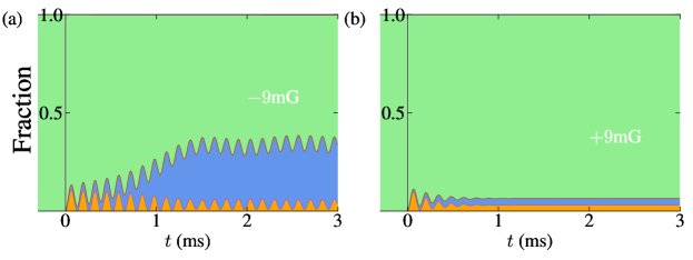
Figure S2: Contrast between the quench dynamics at large negative (panel (a)) and positive ((b)) detuning. Shaded green, blue, and orange regimes represent the atomic condensate, non-condensed pair, and molecular condensate fraction, respectively. Indicated in white are the quenched detuning $\bar{\nu}/\Delta\mu_{m}=B-B_{0}$ (in mG).

We begin with Fig. S2(a) which addresses a sweep from an atomic condensate to rather further to the molecular side of resonance than in Fig. 2(a) in the main text. It is worth concentrating on the detailed time dependence as this shows that in the early stages of the evolution the greatest change is associated with the creation of a molecular condensate. But shortly thereafter the pairing contribution begins to grow. In this case an overall envelope shows that the pairing is growing at the expense of the atomic condensate and this is expected because this sweep is deeper on the molecular side so that the initial atomic condensate is less stable. After a transient, the molecular condensate is frozen and rather time independent except for small oscillations. In addition, there is a three-way coupled oscillation between the atomic and the molecular condensates and the pairs.

If we compare Fig.S2(a) with Fig.S2(b) where the final state of the system is on the atomic side of resonance, it is clear that the molecular condensate and the pairing terms are in this new figure much reduced in magnitude. In panel (b), one sees that the atomic condensate is not as driven to decay, since it is not as unstable as in the previous case. Hence we see fewer pairs. Here, too, one sees after a transient that there is a three-way coupled oscillation.

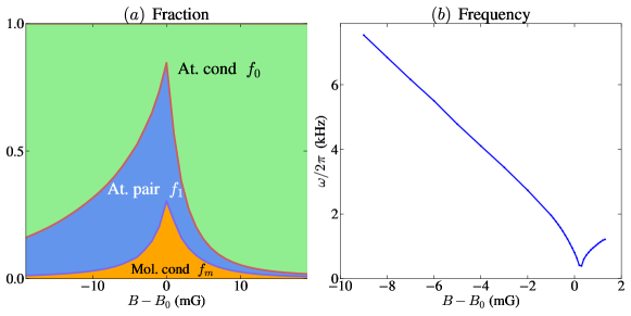
Figure S3: Panel (a) shows the time averaged weight of each of the three components (atomic condensate fraction $f_{0}=|\Psi_{10}|^{2}/n$, non-condensed atom-pair fraction $f_{1}=n_{1}/n$, and molecule fraction $f_{m}=2|\Psi_{20}|^{2}/n$) as a function of the quenched detuning $\bar{\nu}/\Delta\mu_{m}=B-B_{0}$. The results are obtained for the steady state reached after a quench as in Fig. 3(a,b) in the main text. It relates to Fig. 4(b) in the main text by showing the quantities that were not plotted in Fig. 4(b), namely $f_{0}$ and $f_{1}$; the results here could serve as a good basis for predictions to be addressed experimentally in future. (b) This figure plots the steady-state oscillation frequency $\omega$ as a function of the quenched detuning $B-B_{0}$ for fixed particle number density $n=2.9\times 10^{13}$cm^-3.

We next turn to the component contributions for more general situations where the final state detuning is varied continuously. This is plotted in Fig. S3(a). This figure can be compared to Figure 4(b) in the main text. What is most striking here is that while the molecular boson contributions are reasonably symmetric around resonance, the pair contribution is more significant on the molecular side, as already seen in Fig. S2. Indeed, we have argued in the text for such an asymmetry based on energy conservation issues. When the molecular level is far below the atomic level the creation of molecules must be compensated by introducing higher energy states, in this case pairs.

In addition to this asymmetry what is rather interesting here is that there is a re-stabilization of the atomic condensate deep into the molecular side of resonance. This is rather similar to what one would observe in a simple two-level Rabi oscillation.

For completeness, we also show in Fig. S3(b) the steady-state oscillation frequency vs detuning $B-B_{0}$. There is a clear V-shape with a minimum of frequency at $B-B_{0}$ very close to zero, corresponding to the $2$-body resonance, but more precisely at $B-B_{0}\approx 0.25$mG. Here the plot terminates at $B-B_{0}=2$mG, because the oscillations above $2$mG are completely damped.

In summary, given that there is a dichotomy between pairing contributions and condensate-only contributions (but which go beyond the simple two-body Feshbach coupling), it will be important in future to obtain more direct experimental evidence for or against these non-condensed pair effects. Similarly, for future theory it may be important to include direct pair-wise inter-condensate correlations.