Inter-temperature Bandwidth Reduction
in Cryogenic QAOA Machines

Abstract

The bandwidth limit between cryogenic and room-temperature environments is a critical bottleneck in superconducting noisy intermediate-scale quantum computers. This paper presents the first trial of algorithm-aware system-level optimization to solve this issue by targeting the quantum approximate optimization algorithm. Our counter-based cryogenic architecture using single-flux quantum logic shows exponential bandwidth reduction and decreases heat inflow and peripheral power consumption of inter-temperature cables, which contributes to the scalability of superconducting quantum computers.

I Introduction

Quantum computers (QCs) require classical computers (CCs) for their essential control and management to perform quantum computation. Examples of such interactions between quantum devices and CCs include quantum error correction in fault-tolerant quantum computing and classical-quantum hybrid algorithms in noisy intermediate-scale quantum (NISQ) machines, such as Variational Quantum Algorithms (VQAs) and quantum approximate optimization algorithm (QAOA) [1] shown in Fig. 1 (middle). Consequently, QCs need to ensure sufficient bandwidth between a quantum processing unit (QPU) and CCs for essential interactions.

Superconducting qubits operate in a dilution refrigerator, as shown on the left side of Fig. 1, due to their susceptibility to thermal noise. Superconducting QCs (SQCs) use high-frequency coaxial cables for inter-temperature interaction between a room-temperature CC and a cryogenic QPU. The heat inflow from these cables strictly constrains the system volume of SQCs. As the SQC systems scale up, the number of required cables for the interaction also grows, leading to a higher heat inflow through the cables and more power consumption for the peripherals of cables. In addition to the cooling cost required for the QPU itself, this increased heat inflow and peripheral power consumption may exceed the cooling capacity of the refrigerator. In such a case, the thermal noise induces decoherence in the QPU, leading to incorrect computations. Thus, the bandwidth is a critical system parameter as it defines the number of cables or their material.

We propose a concept to compress information within the cryogenic environment to reduce the required inter-temperature bandwidth in SQCs during the NISQ algorithms such as VQAs. To show the effectiveness of our concept, we focus on QAOA, one of the simplest variants of VQAs, as a first step. We analyze the communication behavior of QAOA and propose a novel counter-based cryogenic architecture for it. Our contributions are summarized as follows.

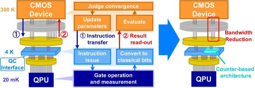
Figure 1: Baseline system design of SQC (left), QAOA procedure (middle), and our proposed system design (right).

1. We analyze the inter-temperature communication of QAOA to identify the bandwidth bottleneck (Sec. III).

2. We propose a new counter-based architecture to reduce the inter-temperature bandwidth and design it with single-flux quantum (SFQ) circuits (Sec. IV).

3. Our evaluation shows that the bandwidth requirement is reduced from $\mathit{O}\left(N\right)$ to $\mathit{O}\left(1\right)$ by using $\mathit{O}\left(\log{N}\right)$-bit counters where $N$ is the number of qubits (Sec. V-A).

4. We discuss the trade-off between the power dissipation of cables and our counter-based architecture (Sec. V-B).

II Background

II-A Quantum approximate optimization algorithm

QAOA[1] is the leading example of VQAs for combinatorial optimization in which the optimization is reduced to the search for ground states of the Hamiltonian of the Ising model

$$H_{C}=-\sum_{i=1}^{N}h_{i}Z_{i}-\sum_{i\neq j}J_{ij}Z_{i}Z_{j},$$ (1)

where $Z_{i}$ represents the spin orientation and $h_{i},J_{ij}$ represents the magnitude of the magnetic field and interaction between spins[2]. The output state of the QAOA circuit is formulated as

$$\Ket{\psi(\bm{\gamma},\bm{\beta})}=e^{-\mathit{i}\beta H_{B}}\left(\prod_{l=1}^{L}U_{B}(\beta_{l})U_{C}(\gamma_{l})\right)\Ket{+}^{\otimes N},$$ (2)

where $U_{C}(\gamma)=e^{-\mathit{i}\gamma H_{C}},U_{B}(\beta)=e^{-\mathit{i}\beta H_{B}}$, and $H_{B}=-\sum_{i=1}^{N}X_{i}$. Note that $\bm{\gamma},\bm{\beta}$ are parameters to optimize.

A significant challenge in the use of QAOA lies in appropriately mapping classical optimization problems into a quantum framework. Mapping such a problem onto the QAOA necessitates a translation process where the objective function and constraints of the optimization problem are reformulated into the Ising model. Intuitively, we can imagine this process as representing each integer decision variable by a set of qubits. For example, in a max cut problem, each spin $Z_{i}$ in Eq. (1) indicates the group to which the $i$-th node of the target graph belongs. See Ref. [3] for more details on mapping combinatorial optimization problems to the Ising model.

II-B Sampling nature of cost function in QAOA

In QAOA, we minimize the expected value of energy $\left\langle{H_{C}}\right\rangle=\Bra{\psi\left(\bm{\gamma},\bm{\beta}\right)}H_{c}\Ket{\psi\left(\bm{\gamma},\bm{\beta}\right)}.$ Since it is impossible to measure this energy directly, we approximate it with the cost function

$$C(\bm{z})=\sum_{i=1}^{N}s_{i}z_{i}+\sum_{i\neq j}c_{ij}\left(z_{i}\oplus z_{j}\right),$$ (3)

which receives the classical bit sequence $\bm{z}\in\left\{0,1\right\}^{N}$ obtained from the quantum state measurement. Note that $s_{i}$ and $c_{ij}$ correspond to $h_{i}$ and $J_{ij}$ in Ising Hamiltonian. We take $T$ times of sampling (trials) and then approximate the energy as

$$\left\langle{H_{C}}\right\rangle\simeq\frac{1}{T}\sum_{t=1}^{T}C(\bm{z}_{t}).$$ (4)

II-C Related work on inter-temperature bandwidth reduction of SQCs

Using cryogenic computing peripherals such as SFQ circuits for peripherals of SQCs has been actively studied[4, 5]. Jokar et al. [4] proposed an SFQ-based qubit control system based on the SIMD concept. While their system focuses on the bandwidth for qubit control, our system mainly concentrates on the measurement readouts based on the bottleneck analysis on Sec. III.

In the field of physics, Opremcak et al. [5] proposed a method for efficient qubit measurements in cryogenic environments by equipping photon detectors on an SFQ chip. Based on such a cryogenic qubit measurement technique, this study presents a system architecture for reducing inter-temperature communications for qubit measurements.

Moreover, to the best of our knowledge, this is the first paper that discusses such algorithm-aware system-level optimization for NISQ machines. Unlike the prior works above [4, 5], we concentrate on application-aware optimization as a new research direction.

III Modeling Communication on QAOA machines

III-A Baseline system design

The left side of Fig. 1 shows the baseline system. We assume that SFQ pulses implement QPU control signals and the inter-temperature communication is digital. The execution flow of QAOA is a repetition of the cycle shown in the center of Fig. 1. Inter-temperature communications occur during \scriptsize{1}⃝ the instruction transfer for QPU control and \scriptsize{2}⃝ the read-out of measurement results as shown in Fig. 2. In the following subsections, we model the required bandwidths of these communications on the baseline system and discuss their major bottleneck.

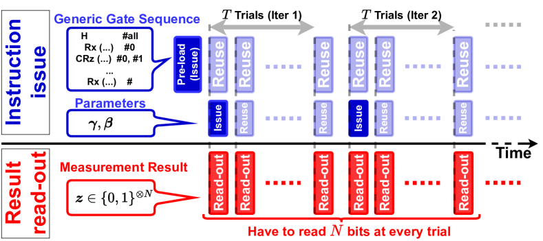
Figure 2: Timing of inter-temperature communication in QAOA

III-B Bandwidth for inter-temperature communication

First, we formulate the execution time of the entire QAOA circuit $t_{QC}$ to model the required bandwidths. The quantum circuit of QAOA repeats the same sequence of gates (which we call a layer) differing only in parameters following the Hamiltonian of Eq. (1) derived from the problem instance. Specifically, for the first- and second-order terms $S,C$ of the Hamiltonian, each layer consists of $S$ $R_{z}$ gates, $C$ entangling blocks ($Ent$ := CNOT-$R_{z}$-CNOT), and $N$ $R_{x}$ gates.

We generally denote the time required to apply a quantum gate $G$ as $t_{G}$. $t_{\text{reset}}$, $t_{\text{init}}$, and $t_{\text{meas}}$ represent the reset, initialization, and measurement operation time per qubit, respectively. We assume the gate level parallelism of one-qubit gates, including measurement, as $P$ and that of two-qubit gates as $P/2$. Then, we model the per-layer execution time $t_{\text{L}}$ and $t_{QC}$ as

$$t_{\text{L}} =St_{R_{z}}+2Ct_{Ent}+Nt_{R_{x}},$$ (5)

$$t_{QC} =\cfrac{Nt_{\text{reset}}+Nt_{\text{init}}+Lt_{\text{L}}+Nt_{\text{meas}}}{P},~{}$$ (6)

where $L$ represents the number of layers per QAOA circuit.

\scriptsize{1}⃝ Bandwidth for instruction transfer: We analyze the locality of instruction transfer communication. Each layer is the same sequence of gates differing only in parameters. Therefore, we need to transfer instructions of a layer only once and can reduce the total number of instruction transfers by treating the generic gate sequence and QAOA parameters separately, as shown in Fig. 2. The layer is consistent throughout the optimization cycle, so it suffices to transfer the layer instructions only once at a low speed before QAOA execution. The following discussion does not consider the layer instruction transfer for the bandwidth analysis because it is short enough relative to $t_{QC}$. The parameters must only be transferred once per circuit parameter update, i.e., once every $T$ trials. Such a buffering functionality is plausible for SFQ circuits by using ring buffers[6].

Based on the discussion above, we model the required bandwidth for the instruction transfer $BW_{\text{inst}}$. Let $b_{p}$ be the bit width of each QAOA parameter. The transfer of $2lb_{p}$ bits of QAOA parameters must be completed before the $l$-th layer operation starts in the first trial, i.e., within $\left(N(t_{\text{reset}}+t_{\text{init}})+(l-1)t_{\text{L}}\right)/P$ in each iteration. The maximum bandwidth requirement is

$$BW_{\text{inst}}=\underset{l\in\left\{1,\cdots,L\right\}}{\text{ max }}\frac{2Plb_{p}}{N\left(t_{\text{reset}}+t_{\text{init}}\right)+(l-1)t_{\text{L}}}$$

$$=\max\left\{\frac{2Pb_{p}}{N\left(t_{\text{reset}}+t_{\text{init}}\right)},\frac{2PLb_{p}}{(L-1)t_{\text{L}}}\right\}.$$ (7)

\scriptsize{2}⃝ Bandwidth for measurement read-out: The required bandwidth for read-out $BW_{\text{meas}}$ can be estimated as $N$ bits per quantum circuit execution, as shown in the of Fig. 3, i.e.,

$$BW_{\text{meas}}=N/t_{QC}=\frac{P}{t_{\text{reset}}+t_{\text{init}}+Lt_{\text{L}}/N+t_{\text{meas}}}.$$ (8)

III-C Attention to measurement bandwidth at design phase

When designing the system, the resources should be sufficient to handle the different problems and parameter settings of the algorithm. Thus, we consider the worst case in terms of bandwidth, i.e., the shortest execution time case.

Equations (7) and (8) both have $t_{\text{L}}$ in the denominator, which depends on $S$ and $C$ and represents the sparseness of the problem. For example, for a maximum cut problem, $C$ corresponds to the number of edges in the graph. In the worst case, these values are $S=0,C=N-1$ because, for the case with $C<N-1$, there exists a qubit that does not entangle, and we can split the problem into smaller problems that do not require $N$ qubits. In this case, $t_{L}$ in Eq. (5) comes to $O(N)$. Also, we assume the number of layers to be $L=1$ for the shortest execution time. Hence, in the worst case, the orders of $BW_{\text{inst}}$ and $BW_{\text{meas}}$ are $O(Pb_{p}/N)$ and $O(P)$, respectively. Given that $b_{p}$, the bit width of the parameters to be optimized, is at most several tens of bits, it results in the inequality $Pb_{p}/N\ll P\iff b_{p}/N\ll 1$ as the number of qubits $N$ scales to $10^{2}$ or larger. Based on these observations, we conclude that the $BW_{\text{meas}}$ is dominant in the inter-temperature bandwidth of the baseline, and the following sections focus on reducing it.

IV Counter-based architecture at the 4-K stage

IV-A Bandwidth reduction with counter-based architecture

In the baseline system, we calculate $\left\langle{H_{C}}\right\rangle$ in Eq. (4) by evaluating $C(\bm{z})$ in Eq. (3) at every trial. Thus, we need inter-temperature communications to send measurement results of $N$ qubits to the room-temperature environment after each trial ends, as shown in Fig. 3. The required bandwidth of the baseline system is $BW_{\text{meas}}=N/t_{QC}$ as explained in Section III.

By contrast, our counter-based system keeps counting values of qubit measurements in a 4-K environment throughout $T$ trials to reduce the inter-temperature communication. We count the number of measurements of ‘1’s in each qubit and the non-zero coefficients in each qubit pair as $C_{i}=\sum_{t=1}^{T}z_{i}^{t}$ and $C_{ij}=\sum_{t=1}^{T}\left(z_{i}^{t}\oplus z_{j}^{t}\right)$, respectively, throughout $T$ trials to calculate the cost function as

$$\left\langle{H_{C}}\right\rangle\simeq\frac{1}{T}\left(\sum_{i=1}^{N}s_{i}C_{i}+\sum_{i\neq j}c_{ij}C_{ij}\right).$$ (9)

In other words, the function $\left\langle{H_{C}}\right\rangle$ is estimated in the sum of products using the counter values after $T$ trials. Assuming that each counter has a sufficient bit width to keep $C_{i}$ and $C_{ij}$ throughout $T$ trials, our method requires only one inter-temperature communication with $M\left\lceil\log_{2}{T}\right\rceil$bits after all $T$ trials. Here, $M$ represents the number of counters in use.

However, applying our method naively could increase the bandwidth requirement rather than the baseline because transferring all the counter values at once may require a larger bandwidth than $BW_{\text{meas}}$. In addition, we cannot assume that the counter bit width is always sufficient as the trial count $T$ changes depending on use cases.

To avoid these problems, we introduce an MSB-sending policy to level the bit transfers across all $T$ trials and suppress the bandwidth requirement. In this policy, we limit each counter entry to $b$ bits ($<\left\lceil\log_{2}{T}\right\rceil$), clear (destructively read) MSBs once every $2^{b-1}$ trials, and then transfer them to the upper stage. As shown in Fig. 3, the CMOS device in the upper stage takes these MSBs as “$2^{b-1}$ counts” and stores them as the upper bits of counters. Hence, the CMOS and SFQ devices cooperatively behave as large-bit-width counters. While this policy requires more than $M\left\lceil\log_{2}{T}\right\rceil$ bits to transfer, it reduces the bandwidth requirement by smoothing out the communication across all $T$ trials rather than transferring all bits at once.

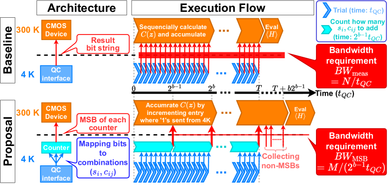
Figure 3: Inter-temperature communication in QAOA using counters

In contrast to the bandwidth of the baseline system $BW_{\text{meas}}=N/t_{\text{QC}}$, in our system, $M$bits of MSBs are transferred once per $2^{b-1}$ trials. Thus, the bandwidth requirement for MSB $BW_{\text{MSB}}$ is just $BW_{\text{MSB}}=M/(2^{b-1}t_{\text{QC}})$. Hence, the bandwidth reduction is exponential to the counter entry $b$.

Note that we can further reduce this bandwidth requirement by adaptively transferring MSBs only when one or more entries are filled with all ‘1’s. However, we use the regular MSB-sending policy to simplify the circuit design in this paper.

IV-B Execution time overhead for collecting non-MSBs

In our method, we collect $bM$ bits remaining on the SFQ counters after all $T$ trials to complete the cost evaluation. Suppose that we collect these bits within $t_{C}$. The bandwidth requirement for the non-MSBs collecting $BW_{\text{non-MSB}}$ equals $bM/t_{C}$. Hence, the bandwidth of our system, $BW_{\text{proposed}}$, is

$$BW_{\text{proposed}}=\max{\left(BW_{\text{MSB}},\hskip 3.0ptBW_{\text{non-MSB}}\right)}.$$ (10)

To keep $BW_{\text{non-MSB}}$ as small as $BW_{\text{MSB}}$, $t_{C}$ must be long enough to satisfy $t_{C}\geq b2^{b-1}t_{\text{QC}}$. Hence, our method has a trade-off between the bandwidth reduction and the execution time overhead; the bandwidth reduction is exponential to $b$ while the execution time grows from $Tt_{\text{QC}}$ to $(T+b2^{b-1})t_{\text{QC}}$.

IV-C Configuration of counters with SFQ circuit

We designed our counter-based architecture using the existing RSFQ cell library [7], and Fig. 4 shows the circuit diagram, the number of JJs, and the total bias current per counter entry. Note that we estimated the bias current of the inhibit cell from the number of JJs because it is not presented in Ref. [8].

The counter module consists of $N(N+1)/2$ counters. Each bit consists of a T-flipflop (TFF) except for the MSB, which uses a D-flipflop (DFF).

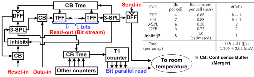
Figure 4: Detailed configuration of a counter entry

During the execution of the quantum circuit, pulses are routed round-robin to the $N(N+1)/2$ “send” lines to achieve communication smoothing in the MSB-sending policy.

In the non-MSB collection phase, the reset signal is routed to each counter, and a bit stream is generated on the read-out line. Assuming the counter has a value $v$, this bit stream consists of $2^{b}-v$ ‘1’s and stops when a pulse is routed to the inhibit cell [8] after the counter overflows. This bit stream has $\mathit{O}\left(2^{b}\right)$ length, and sending it as is increases the bandwidth. Therefore, we first route it to a T1 counter[9], which allows bit-parallel read, placed after the CB tree and shared among all counter entries. Here, we can perform this routing by triggering each counter sequentially; thus, only one T1 counter is sufficient. Our design requires only one reset signal per counter, while clock and read-out trees are needed to use bit-parallel readable T1 counters for all counter entries.

V Evaluation

V-A Trade-off between bandwidth and execution time

As discussed in Sec. IV-B, the execution time of QAOA in our proposed system gets $1+b2^{b-1}/T$ times longer than that of the baseline system, Here, we study how large we can set $b$ within an acceptable execution time overhead $r$. In other words, we evaluate how much bandwidth we can reduce with an increased execution time by a factor of $1+r$. The counter bit width $b$ must satisfy

$$\frac{b2^{b-1}}{T}<r\hskip 5.69054pt\Leftrightarrow\hskip 5.69054ptb2^{b}<2rT.$$ (11)

As discussed in Sec. III-B, we consider the worst case ($M=N-1$). The bandwidth ratio between the proposed and baseline is $\cfrac{BW_{\text{proposed}}}{BW_{\text{meas}}}=\cfrac{M/2^{b-1}t_{QC}}{Nt_{QC}}\simeq\cfrac{1}{2^{b-1}}$. Figure 5 (a) shows the bandwidth ratio achieved by maximizing $b$ under Eq. (11) at a certain value of $r$. Note that each plot of Fig. 5 (a) has a staircase shape because the number of bits in the counter $b$ is an integer. Our proposed system works well for larger $T$. For example, when the acceptable execution time overhead is 5% ($r=0.05$), the proposed system reduces the bandwidth by $99.993$% with $T=10^{7}$ and $b=15$, or $87.5$% ($b=4$) with $T=10^{3}$ and $b=4$.

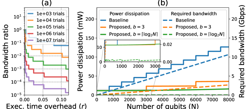
Figure 5: (a) Bandwidth reduction to execution time overhead and (b) power dissipations of baseline and proposed systems.

$T$ is the number of samplings to approximate the quantum state and note that it is still unknown how many samplings are required for QAOA to find a good solution. Here, all the $T$ values shown in Fig. 5 (a) are within $\mathit{O}\left(N\right)$ to $\mathit{O}\left(N^{3}\right)$ as we assume NISQ machines with qubits on the order of $10^{2}$ to $10^{3}$.

V-B Impact on the scalability of the number of qubits

First, we show the bandwidth reduction achieved by the SFQ counters with fixed or $O(\log{N})$-size bit lengths. As discussed in Sec. III-C, the bandwidth requirement of the baseline system is $\mathit{O}\left(P\right)$, i.e., proportional to the gate parallelism. On the other hand, that of our system is $\mathit{O}\left(P/2^{b}\right)$ as demonstrated in Sec. V-A with a certain time overhead $r$ according to Eq. (11). Considering the worst case for the bandwidth with $P=N$ (fully parallelized) and using parameters described in references [4, 5] as $t_{\text{reset}}=100$ ns, $t_{\text{init}}=t_{R_{x}}=t_{R_{z}}=10$ ns, $t_{CNOT}=60$ ns, and $t_{\text{meas}}=380$ ns, respectively, $t_{QC}$ in Eq. (6) is estimated as $t_{QC}\simeq 100\times 1+10\times 3+60\times 4+380\times 1=750$ ns. Using the $t_{QC}$ value, Fig. 5 (b) shows the required bandwidths of the baseline and our system ($b=3$) as blue and orange dashed lines, respectively. Furthermore, our system can reduce the required bandwidth to $\mathit{O}\left(1\right)$ by setting $b=\left\lceil\log{N}\right\rceil$ (green dashed line in the figure, see the enlarged view). Note that we assume $BW_{\text{MSB}}$ is dominant for the proposed system’s bandwidth in this evaluation, i.e., Fig. 5 (b) does not care about $r$ in Sec. V-A.

Next, we evaluate the trade-off between heat inflow through cables and power consumption in a cryogenic environment with our system. We suppose that the systems have stainless steel coaxial cables (UT085 SS-SS) between the 4-K and upper stages, and its heat inflow is 1.0 mW as in Tab. 2 of Ref. [10]. In addition to the heat inflow, we consider the power consumption of the cable peripherals. We assume the amplifier, which is the main source of peripheral power consumption, is LNF-LNC4_8C as in Ref. [10], and its power consumption is 10.5 mW per cable according to its datasheet. The bandwidth per cable is assumed to be 1 Gbps, and the system has a sufficient number of cables to exceed its required bandwidth (e.g., the system whose bandwidth requirement is 2.5 Gbps has three cables).

Based on the RSFQ design in Sec. IV-C and the ERSFQ power model in Ref. [11], we estimate the power consumption of our system when ERSFQ is applied. Here, the power of the counter, $P_{\text{counter}}$, with ERSFQ can be estimated as $P_{\text{counter}}=(\text{bias current})\times(\text{frequency})\times\Phi_{0}\times 2$. We use flux quantum $\Phi_{0}$ of $2.068$ fWb, and the counter is assumed to operate at 1.33 MHz, the reciprocal of $t_{QC}=750$ ns. As a result, $P_{\text{counter}}$ is $(9.71b+16.8)$ pW.

Table I summarizes the configuration of cables and our SFQ counter, and Fig. 5 (b) compares the power dissipations (sum of heat inflow and power consumption) between the baseline and proposed systems. While that of the baseline is dominated by cables as the bandwidth increases, the proposed system reduces the impact of cables by reducing the bandwidth with the negligible overhead of counters. Our system achieved lower power dissipation than the baseline on QAOA machines with more than 750 qubits.

Note that our method focuses on cables between 300 K and 4 K environments and does not change the number of cables between 4 K and 20 mK. Consequently, the power consumption of our architecture remains as in Tab. I, without causing additional heat transfer.

The essential advantages of our method are the exponential bandwidth reduction and power consumption of the order of pW. While the evaluation of this paper utilizes a particular cable and peripheral, our method is expected to work well across a variety of system designs because of its general advantages.

TABLE I: Configuration of cables and SFQ counters

	Power dissipation	Configuration
Coaxial cable	Heat inflow: 1.0 mW[10] Periphelars: 10.5 mW[10]	One cable per 1 Gbps
SFQ counter	$(9.71b+16.8)$ pW	$M=N(N+1)/2$ ERSFQ (Freq. = 1.33 MHz )

VI Conclusion and future work

We proposed a general concept of information compression within the cryogenic environment to reduce inter-temperature communication for NISQ machines. To show its effectiveness, we targeted QAOA as a first step. We modeled the inter-temperature communication in QAOA and proposed a bandwidth-efficient counter architecture with SFQ circuits. Our method reduces the communication by transferring the MSB of each counter that tallies the number of additions of each cost function term throughout trials. It successfully reduced the required bandwidth exponentially and decreased heat inflow and peripheral power consumption of coaxial cables in a cryogenic environment with the negligible overhead of SFQ counters.

Computations involving general VQAs often require a vast array of information compared to QAOA. Our concept of information compression using counters is expected to work effectively even in general VQAs; however, a straightforward implementation of a counter architecture capable of concurrently storing all the information required for general VQAs is inefficient and not feasible from a hardware standpoint. Our future work is to propose practical strategies, such as sampling a subset of the information with counters, and apply them to the proposed architecture to support general VQAs.

References

- [1] E. Farhi et al., “A Quantum Approximate Optimization Algorithm,” 2014. [Online]. Available: https://arxiv.org/abs/1411.4028
- [2] T. Inagaki et al., “A coherent Ising machine for 2000-node optimization problems,” Science, vol. 354, no. 6312, pp. 603–606, 2016.
- [3] S. Xie et al., “Ising-CIM: A Reconfigurable and Scalable Compute Within Memory Analog Ising Accelerator for Solving Combinatorial Optimization Problems,” IEEE J. Solid-State Circuits, vol. 57, no. 11, pp. 3453–3465, 2022.
- [4] M. R. Jokar et al., “DigiQ: A Scalable Digital Controller for Quantum Computers Using SFQ Logic,” in Proc. of HPCA, 2022, pp. 400–414.
- [5] A. Opremcak et al., “High-Fidelity Measurement of a Superconducting Qubit Using an On-Chip Microwave Photon Counter,” Phys. Rev. X, vol. 11, p. 011027, Feb 2021.
- [6] K. Ishida et al., “32 GHz 6.5 mW gate-level-pipelined 4-bit processor using superconductor single-flux-quantum logic,” in Proc. of Symp. VLSI Circuits, 2020, pp. 1–2.
- [7] Y. Yamanashi et al., “100 GHz demonstrations based on the single-flux-quantum cell library for the 10 kA/cm2 Nb multi-layer process,” IEICE Trans. Electron., vol. 93, no. 4, pp. 440–444, 2010.
- [8] G. Tzimpragos et al., “A Computational Temporal Logic for Superconducting Accelerators,” in Proc. of ASPLOS, 2020, p. 435–448.
- [9] S. Polonsky et al., “Single flux, quantum B flip-flop and its possible applications,” IEEE Trans. Appl. Supercond., vol. 4, no. 1, pp. 9–18, 1994.
- [10] S. Krinner et al., “Engineering cryogenic setups for 100-qubit scale superconducting circuit systems,” EPJ Quantum Technol., vol. 6, no. 1, p. 2, 2019.
- [11] O. A. Mukhanov, “Energy-Efficient Single Flux Quantum Technology,” IEEE Trans. Appl. Supercond., vol. 21, no. 3, pp. 760–769, 2011.