Towards Efficient and Effective Adaptation of Large Language Models for Sequential Recommendation

Abstract

In recent years, with large language models (LLMs) achieving state-of-the-art performance in context understanding, increasing efforts have been dedicated to developing LLM-enhanced sequential recommendation (SR) methods. Considering that most existing LLMs are not specifically optimized for recommendation tasks, adapting them for SR becomes a critical step in LLM-enhanced SR methods. Though numerous adaptation methods have been developed, it still remains a significant challenge to adapt LLMs for SR both efficiently and effectively. To address this challenge, in this paper, we introduce a novel side sequential network adaptation method, denoted as $\mathop{\mathtt{SSNA}}\limits$, for LLM-enhanced SR. $\mathop{\mathtt{SSNA}}\limits$ features three key designs to allow both efficient and effective LLM adaptation. First, $\mathop{\mathtt{SSNA}}\limits$ learns adapters separate from LLMs, while fixing all the pre-trained parameters within LLMs to allow efficient adaptation. In addition, $\mathop{\mathtt{SSNA}}\limits$ adapts the top-$a$ layers of LLMs jointly, and integrates adapters sequentially for enhanced effectiveness (i.e., recommendation performance). We compare $\mathop{\mathtt{SSNA}}\limits$ against five state-of-the-art baseline methods on five benchmark datasets using three LLMs. The experimental results demonstrate that $\mathop{\mathtt{SSNA}}\limits$ significantly outperforms all the baseline methods in terms of recommendation performance, and achieves substantial improvement over the best-performing baseline methods at both run-time and memory efficiency during training. Our analysis shows the effectiveness of integrating adapters in a sequential manner. Our parameter study demonstrates the effectiveness of jointly adapting the top-$a$ layers of LLMs.

Introduction

Sequential recommendation (SR) aims to predict and recommend the next item of users’ interest using their historical interactions. It has been drawing increasing attention from the research community due to its wide applications in online retail, video streaming and tourism planning, etc. Recently, as large language models (LLMs) have demonstrated state-of-the-art performance in context understanding (OpenAI 2023), numerous efforts have been dedicated to developing LLM-enhanced SR methods (Yuan et al. 2023; Hou et al. 2022). The key idea behind these methods is to leverage LLMs to generate expressive item embeddings from item texts (e.g., titles) for better recommendation. Given that existing LLMs are generally recommendation-independent, adapting LLMs for recommendation tasks becomes an important step in LLM-enhanced SR methods.

There are broadly two categories of methods in adapting LLMs for SR (Yuan et al. 2023). The first category of methods, referred to as top tuning ($\mathop{\mathtt{TT}}\limits$), adapts LLMs by learning an adapter on top of the LLM as illustrated in Figure 1(a). $\mathop{\mathtt{TT}}\limits$ allows efficient adaptation as it does not require both forward and backward propagation across LLMs in training if the outputs of LLMs (i.e., $\mathbf{h}^{n}_{i}$) for each item text are pre-calculated. However, $\mathop{\mathtt{TT}}\limits$ could suffer from limited effectiveness (i.e., recommendation performance) as it is essentially equivalent to adapting only the top layer of LLMs. As suggested in the literature (Shim, Choi, and Sung 2021), different Transformer layers (Vaswani et al. 2017) in LLMs could capture diverse semantics in item texts. Thus, adapting only the top layer could lose valuable information in other layers, leading to sub-optimal recommendation performance. Conversely, the second category of methods, denoted as multi-layer tuning ($\mathop{\mathtt{MLT}}\limits$), enables effective adaptation by adapting potentially all the layers in LLMs via fine-tuning or parameter-efficient fine-tuning (PEFT) (He et al. 2021). Nevertheless, both fine-tuning and PEFT methods are notoriously computation-intensive (Liao, Tan, and Monz 2023). Consequently, $\mathop{\mathtt{MLT}}\limits$ significantly underperforms $\mathop{\mathtt{TT}}\limits$ in terms of efficiency (Yuan et al. 2023). Figure 1(b) illustrates $\mathop{\mathtt{MLT}}\limits$ in which LLMs are adapted using PEFT.

With the prosperity of LLM-enhanced SR methods, developing both efficient and effective LLM adaptation methods for SR has emerged as a critical research challenge. To tackle this challenge, in this paper, we introduce a novel side sequential network adaptation method, denoted as $\mathop{\mathtt{SSNA}}\limits$, for SR. $\mathop{\mathtt{SSNA}}\limits$ features three key designs. First, $\mathop{\mathtt{SSNA}}\limits$ learns adapters separate from LLMs, and keeps all the pre-trained parameters within LLMs fixed. As a result, similar to $\mathop{\mathtt{TT}}\limits$, with pre-calculated outputs from LLMs (e.g., $\mathbf{h}_{i}^{n}$), $\mathop{\mathtt{SSNA}}\limits$ could avoid forward and backward propagation across LLMs during training, and thus, enable efficient adaptation. Second, distinct from $\mathop{\mathtt{TT}}\limits$ that adapts only the top layer of LLMs, $\mathop{\mathtt{SSNA}}\limits$ adapts the top-$a$ layers jointly to allow effective adaptation. Third, $\mathop{\mathtt{SSNA}}\limits$ integrates adapters sequentially via a gated recurrent unit ($\mathop{\mathtt{GRU}}\limits$) network for better effectiveness. As illustrated in Figure 1(b), $\mathop{\mathtt{MLT}}\limits$ adds adapters within each layer of LLMs. This design inherently integrates adapters in a sequential manner. As will be shown in our analysis (Table 8), the sequential integration of adapters significantly contributes to the effectiveness. Thus, $\mathop{\mathtt{SSNA}}\limits$ learns an additional $\mathop{\mathtt{GRU}}\limits$ network to sequentially integrate the adapters, thereby enhancing recommendation performance.

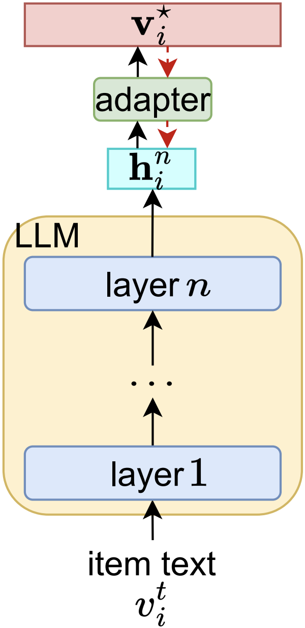
(a) $\mathop{\mathtt{TT}}\limits$

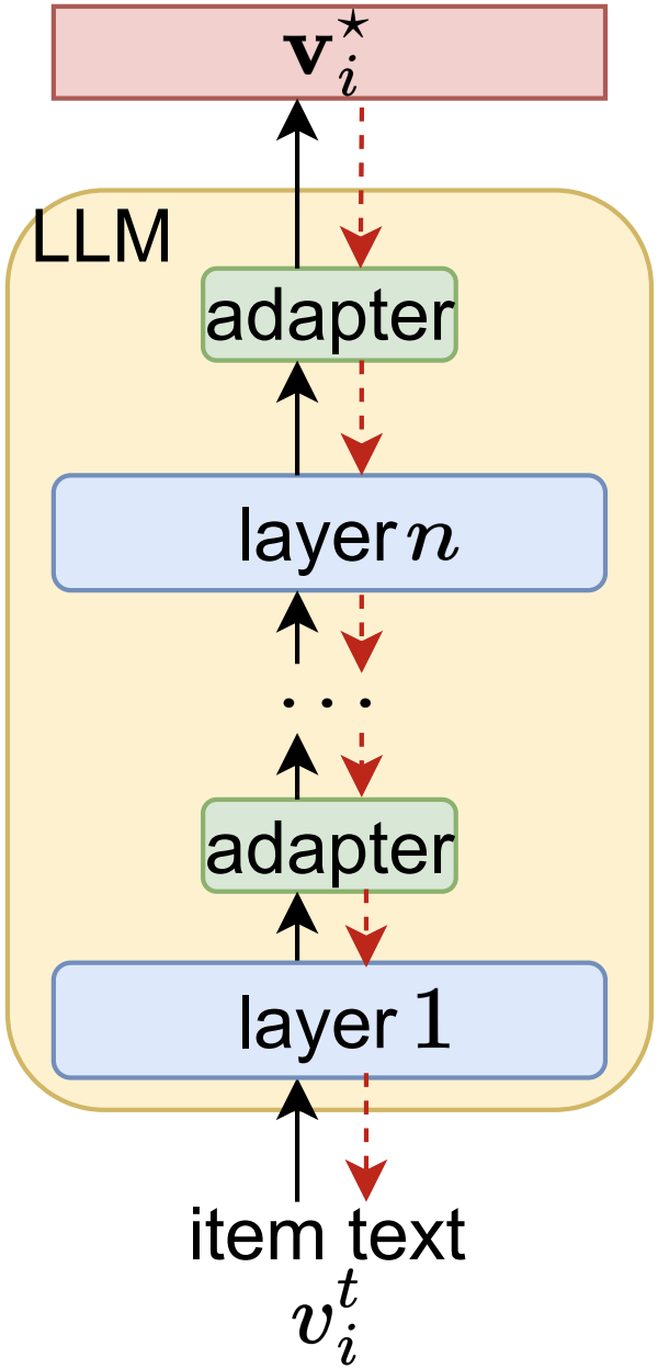
(b) $\mathop{\mathtt{MLT}}\limits$

Figure 1: Illustration of $\mathop{\mathtt{TT}}\limits$ (left) and $\mathop{\mathtt{MLT}}\limits$ (right). In this figure, $\mathbf{h}^{n}_{i}$ is the embedding generated from the LLM using $v_{i}^{t}$; and $\mathbf{v}_{i}^{\star}$ is the adapted item embedding. This figure shares the same legend as Figure 2.

We compare $\mathop{\mathtt{SSNA}}\limits$ against five state-of-the-art baseline methods on five benchmark datasets using three LLMs. The experimental results demonstrate that $\mathop{\mathtt{SSNA}}\limits$ allows both efficient and effective LLM adaptation for SR. Particularly, $\mathop{\mathtt{SSNA}}\limits$ outperforms all the baseline methods across the three LLMs with a remarkable average improvement of as much as 8.5% compared to the best-performing baseline method over the benchmark datasets. $\mathop{\mathtt{SSNA}}\limits$ also achieves remarkable improvement in terms of run-time efficiency (e.g., 30.8x speedup) and memory efficiency (e.g., 97.7% reduction in GPU memory usage) compared to the best-performing $\mathop{\mathtt{MLT}}\limits$ methods. Our analysis and parameter study demonstrates the effectiveness of integrating adapters sequentially, and the effectiveness of adapting top-$a$ layers of LLMs together, respectively. For better reproducibility, we release the processed datasets and the source code in Google Drive .

Related Work

Sequential Recommendation

Numerous SR methods have been developed in the last few years, particularly, leveraging neural networks and attention mechanisms. For example, Hidasi et al. (Hidasi et al. 2015) utilizes $\mathop{\mathtt{GRUs}}\limits$ to capture users’ latent intent from their historical interactions. Tang et al. (Tang and Wang 2018) leverages a convolutional neural network ($\mathop{\mathtt{CNN}}\limits$) to capture the union-level patterns among items for better user intent modeling. Besides neural networks, attention mechanisms have also been widely employed for SR. Ma et al. (Ma, Kang, and Liu 2019) learns attention weights to differentiate the importance of items, enhancing the estimate of users’ intent. Kang et al. (Kang and McAuley 2018) develops a self-attention-based SR method $\mathop{\mathtt{SASRec}}\limits$, in which self-attention mechanisms are utilized to capture the interactions between individual items for better user intent modeling.

Recently, increasing efforts have been dedicated to incorporating LLMs for SR. For example, Hou et al. (Hou et al. 2022) adapts the top layer of LLMs for SR using the mixture-of-expert mechanism ($\mathop{\mathtt{TMoE}}\limits$), and learns transferable recommendation models based on the adapted item embeddings. Yuan et al. (Yuan et al. 2023) shows that item embeddings generated from LLMs could be more expressive than those learned solely based on user interactions, and thus, lead to better recommendation performance. Yuan et al. (Yuan et al. 2023) also shows that adapting the top layer of LLMs using multilayer perceptrons ($\mathop{\mathtt{TMLP}}\limits$) underperforms $\mathop{\mathtt{MLT}}\limits$ methods by a considerable margin.

Parameter-efficient Fine-tuning (PEFT)

As LLMs have demonstrated impressive performance in context understanding, numerous PEFT methods have been developed to adapt LLMs for specific tasks in a parameter-efficient manner. Particularly, Hu et al. (Hu et al. 2021) develops a low-rank adaptation method $\mathop{\mathtt{LoRA}}\limits$, which learns rank decomposition matrices in each LLM layer, while fixing all the pre-trained parameters within LLMs for PEFT. Zaken et al. (Zaken, Ravfogel, and Goldberg 2021) develops $\mathop{\mathtt{BitFit}}\limits$, in which only the bias-terms of LLMs are adapted for the task of interest. Zhang et al. (Zhang et al. 2023) develops $\mathop{\mathtt{ADA}}\limits$, which captures the importance of the pre-trained parameters within LLMs, and prioritizes the adaptation of parameters based on their importance.

Definition and Notations

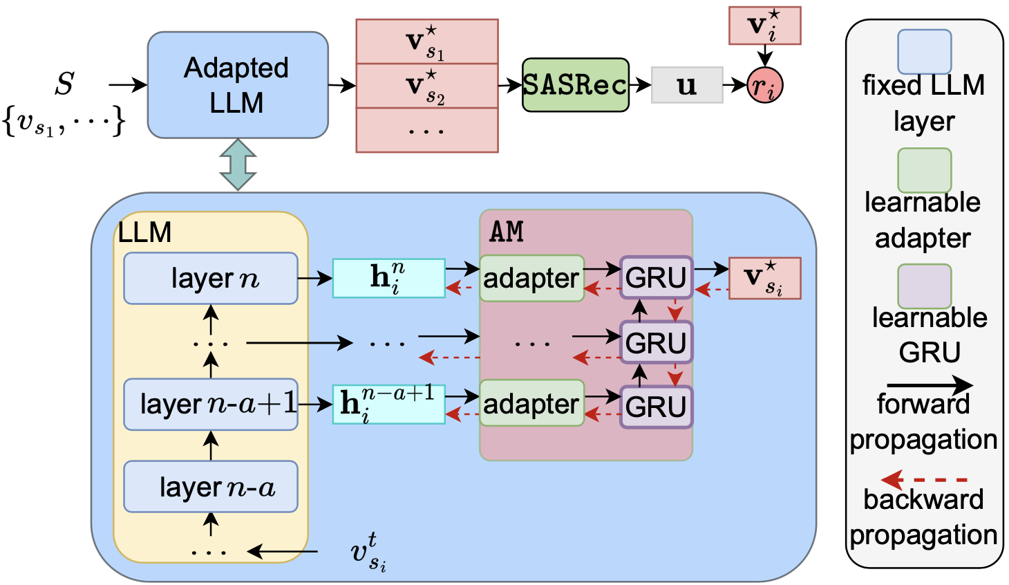
Figure 2: Overall Architecture of $\mathop{\mathtt{SSNA}}\limits$. $\mathop{\mathtt{SSNA}}\limits$ jointly adapts the top-$a$ layers of LLMs, and integrates adapters sequentially using a GRU network for effective adaptation. In addition, $\mathop{\mathtt{SSNA}}\limits$ could avoid forward and backward propagation across LLMs to enable efficient adaptation if the outputs of LLMs (e.g., $\mathbf{h}_{i}^{n}$, $\mathbf{h}_{i}^{n-1}$) are pre-calculated.

In this paper, we denote the set of all the users as $\mathbb{U}=\{u_{1},u_{2},\cdots\}$, where $u_{j}$ is the $j$-th user and $|\mathbb{U}|$ is the total number of users. We also denote the set of all the items as $\mathbb{V}=\{v_{1},v_{2},\cdots\}$, where $v_{i}$ is the $i$-th item and $|\mathbb{V}|$ is the total number of items. We denote the text (e.g., title) of $v_{i}$ as $v_{i}^{t}$. In this paper, we represent the historical interactions of $u_{j}$ as a sequence $S_{j}=\{v_{s_{1}}(j),v_{s_{2}}(j),\cdots\}$ in which $v_{s_{t}}(j)$ is the $t$-th interacted item in $S_{j}$. Given $S_{j}$, we denote the ground-truth next item with which $u_{j}$ will interact as $v_{g}(j)$. When no ambiguity arises, we will eliminate $j$ in $S_{j}$, $v_{s_{t}}(j)$ and $v_{g}(j)$. We use uppercase letters to denote matrices, lower-case bold letters to denote row vectors and lower-case non-bold letters to represent scalars.

Method

Figure 2 presents the overall architecture of $\mathop{\mathtt{SSNA}}\limits$. As shown in Figure 2, $\mathop{\mathtt{SSNA}}\limits$ adapts LLMs by learning adapters for each of the top-$a$ layers of LLMs. Different from that in $\mathop{\mathtt{MLT}}\limits$, the adapters in $\mathop{\mathtt{SSNA}}\limits$ are separate from LLMs to allow efficient adaptation. $\mathop{\mathtt{SSNA}}\limits$ also learns a $\mathop{\mathtt{GRU}}\limits$ network to sequentially integrate the adapters for enhanced recommendation performance. In what follows, we present $\mathop{\mathtt{SSNA}}\limits$ in detail.

LLM Adaptation

$\mathop{\mathtt{SSNA}}\limits$ learns an adaptation module ($\mathop{\mathtt{AM}}\limits$) to adapt LLMs for SR, while fixing all the pre-trained parameters within LLMs. Particularly, $\mathop{\mathtt{AM}}\limits$ comprises $a$ adapters to adapt the top-$a$ layers of LLMs. $\mathop{\mathtt{AM}}\limits$ also includes a $\mathop{\mathtt{GRU}}\limits$ network to integrate these adapters sequentially.

Adapter Design

Existing work (Yuan et al. 2023; Wang et al. 2022) typically implements adapters using multilayer perceptrons (MLPs). However, as suggested in a recent work (Chen et al. 2022), mixture-of-export mechanisms (MoEs) (Shazeer et al. 2017) could better capture the clustering structures within items compared to MLPs, enabling more expressive item embeddings. Thus, $\mathop{\mathtt{SSNA}}\limits$ implements adapters using MoEs. Specifically, each adapter in $\mathop{\mathtt{SSNA}}\limits$ comprises a projection layer and a routing layer. Within each projection layer, $\mathop{\mathtt{SSNA}}\limits$ has $n_{p}$ projection heads. $\mathop{\mathtt{SSNA}}\limits$ implements each projection head using parametric whitening (Huang et al. 2021) as follows:

$$\mathbf{e}^{m}_{i}(k)=\left(\mathbf{h}_{i}^{n-m}-\mathbf{b}^{m}_{k}\right)W^{m}_{k},$$ (1)

where $\mathbf{h}_{i}^{n-m}$ is the embedding of item text $v_{i}^{t}$ generated from the $(n\text{-}m)$-th layer of the LLM ($m\in\{0,1,\cdots,a\text{-}1\}$), and $\mathbf{e}^{m}_{i}(k)$ is the projected embedding from the $k$-th projection head of the $m$-th adapter. $\mathbf{b}^{m}_{k}$ is a learnable shift parameter, and $W_{k}^{m}$ is a learnable projection parameter.

$\mathop{\mathtt{SSNA}}\limits$ utilizes a Gaussian routing to aggregate the projected embedding from each projection head as follows:

$$\mathbf{z}_{i}^{m}=\text{Softmax}(\boldsymbol{\alpha}_{i}^{m})[\mathbf{e}_{i}^{m}(1);\mathbf{e}_{i}^{m}(2);\cdots;\mathbf{e}_{i}^{m}(n_{p})],$$ (2)

where $\mathbf{z}_{i}^{m}$ is the output from the $m$-th adapter, and $\boldsymbol{\alpha}_{i}^{m}\sim\mathcal{N}(\boldsymbol{\mu}_{i}^{m},\text{diag}((\boldsymbol{\sigma}_{i}^{m})^{2}))$ is the weights learned to aggregate the projected embeddings. $\mathop{\mathtt{SSNA}}\limits$ parameterizes the mean $\boldsymbol{\mu}_{i}^{m}$ and standard deviation $\boldsymbol{\sigma}_{i}^{m}$ of the Gaussian distribution as follows:

$$\boldsymbol{\mu}^{m}_{i}=\mathbf{h}_{i}^{n-m}B^{m}\;\text{and}\;\boldsymbol{\sigma}^{m}=\text{Softplus}(\mathbf{h}_{i}^{n-m}U^{m}),$$ (3)

where Softplus is the activation function to enable a positive standard deviation; $B^{m}$ and $U^{m}$ are learnable parameters in the $m$-th adapter.

Sequential Integration of Adapters

As shown in Figure 2, $\mathop{\mathtt{SSNA}}\limits$ learns a $\mathop{\mathtt{GRU}}\limits$ network to sequentially integrate the adapters as follows:

$$\mathbf{v}_{i}^{\star}=\mbox{$\mathop{\mathtt{GRU}}\limits$}(\mbox{$\mathop{\mathtt{GRU}}\limits$}(\mbox{$\mathop{\mathtt{GRU}}\limits$}(\mathbf{0},\mathbf{z}_{i}^{0}),\mathbf{z}_{i}^{1})\cdots,\mathbf{z}_{i}^{a-1}),$$ (4)

where $\mathbf{v}_{i}^{\star}$ is the adapted embedding for item $v_{i}$. We initiate the memory cell in $\mathop{\mathtt{GRU}}\limits$ with a zero vector $\mathbf{0}$ following the literature (Hidasi et al. 2015). As illustrated in Figure 1(b), $\mathop{\mathtt{MLT}}\limits$ stacks adapters inside LLMs, and thus, inherently integrates adapters in a sequential manner. Our own analysis (Table 8) demonstrates that this property could significantly contribute to the recommendation performance. Thus, besides adapters, $\mathop{\mathtt{SSNA}}\limits$ learns an additional GRU network to sequentially integrate the adapters for enhanced recommendation performance.

User Intent Modeling and Recommendation Generation

We utilize the widely used $\mathop{\mathtt{SASRec}}\limits$ model (Kang and McAuley 2018) in $\mathop{\mathtt{SSNA}}\limits$ to capture users’ intent and generate recommendations. Specifically, given the interaction sequence of user $u_{j}$: $S_{j}=\{v_{s_{1}}(j),v_{s_{2}}(j),\cdots\}$, we generate adapted embeddings for each of the interacted items, and stack these embeddings to generate an embedding matrix for $S_{j}$ as follows:

$$M_{j}=[\mathbf{v}_{s_{1}}^{\star}(j);\mathbf{v}_{s_{2}}^{\star}(j);\cdots],$$ (5)

where $\mathbf{v}_{s_{t}}^{\star}(j)$ is the adapted embedding of item $v_{s_{t}}(j)$. Given $M_{j}$, we model users’ intent using $\mathop{\mathtt{SASRec}}\limits$:

$$\mathbf{u}_{j}=\mbox{$\mathop{\mathtt{SASRec}}\limits$}(M_{j}),$$ (6)

where $\mathbf{u}_{j}$ represents the intent of user $u_{j}$. With $\mathbf{u}_{j}$, the recommendation score of item $v_{i}$ is calculated as follows:

$$r_{ij}=\cos(\mathbf{u}_{j},{\mathbf{v}_{i}^{*}}),$$ (7)

where $\cos(\cdot)$ is the cosine similarity and $r_{ij}$ is the recommendation score of $u_{j}$ on $v_{i}$. $\mathop{\mathtt{SSNA}}\limits$ recommends the top-$k$ items of the highest recommendation scores.

Network Training

We utilize the cross-entropy objective function to minimize the negative log-likelihood of correctly recommending the ground truth next item as follows:

$$\min\limits_{\boldsymbol{\Theta}}\sum_{u_{j}\in\mathbb{U}}\frac{\exp(\cos(\mathbf{u}_{j},\mathbf{v}_{g}^{*}(j))/\tau)}{\sum_{v_{i}\in\mathbb{N}_{j}}\exp(\cos(\mathbf{u}_{j},\mathbf{v}_{i}^{*})/\tau)},$$ (8)

where $\mathbb{U}$ is the set of all the users; $\boldsymbol{\Theta}$ is the set of learnable parameters in $\mathop{\mathtt{SSNA}}\limits$ (i.e., parameters in $\mathop{\mathtt{AM}}\limits$ and $\mathop{\mathtt{SASRec}}\limits$); $\exp(\cdot)$ is the exponential function; $\mathbf{v}_{g}^{*}(j)$ is the adapted embedding of the ground-truth next item of $u_{j}$; $\mathbb{N}_{j}$ is the set of randomly sampled negative items of $u_{j}$; $\tau$ is a hyper-parameter to scale the cosine similarities (Hou et al. 2022). $\mathop{\mathtt{SSNA}}\limits$ minimizes the objective function using batch optimizations. For $u_{j}$ within a particular batch, $\mathop{\mathtt{SSNA}}\limits$ regards the ground-truth next items from all other users in the same batch as the set of negative items (i.e., $\mathbb{N}_{j}$) of $u_{j}$. All the learnable parameters are randomly initialized, and are optimized in an end-to-end manner.

Materials

Baseline Methods

We compare $\mathop{\mathtt{SSNA}}\limits$ against five state-of-the-art baseline methods. Specifically, we compare $\mathop{\mathtt{SSNA}}\limits$ with the state-of-the-art $\mathop{\mathtt{MLT}}\limits$ methods $\mathop{\mathtt{LoRA}}\limits$ (Hu et al. 2021), $\mathop{\mathtt{ADA}}\limits$ (Zhang et al. 2023), and full fine-tuning ($\mathop{\mathtt{Full}}\limits$) (Yuan et al. 2023). Besides $\mathop{\mathtt{MLT}}\limits$ methods, we also compare $\mathop{\mathtt{SSNA}}\limits$ with $\mathop{\mathtt{TT}}\limits$ methods: $\mathop{\mathtt{TMLP}}\limits$ (Yuan et al. 2023) and $\mathop{\mathtt{TMoE}}\limits$ (Hou et al. 2022), in which MPLs and MoEs are utilized to implement the adapter, respectively. We refer the audience of interest to the Section “Related Work” for details of the baseline methods.

$\mathop{\mathtt{LoRA}}\limits$ and $\mathop{\mathtt{ADA}}\limits$ have demonstrated superior performance over a comprehensive set of other methods such as $\mathop{\mathtt{BitFit}}\limits$ (Zaken, Ravfogel, and Goldberg 2021). Thus, we compare $\mathop{\mathtt{SSNA}}\limits$ with $\mathop{\mathtt{LoRA}}\limits$ and $\mathop{\mathtt{ADA}}\limits$ instead of the methods that they outperform. For $\mathop{\mathtt{LoRA}}\limits$ and $\mathop{\mathtt{ADA}}\limits$, we use the implementation in PEFT (Mangrulkar et al. 2022), a widely used library for parameter-efficient fine-tuning. We implement $\mathop{\mathtt{Full}}\limits$, $\mathop{\mathtt{TMLP}}\limits$ and $\mathop{\mathtt{TMoE}}\limits$ using Pytorch-lighting and Transformers (Wolf et al. 2020). Transformers is a prevalent library for fine tuning LLMs. For a fair comparison, we employ $\mathop{\mathtt{SASRec}}\limits$, the user intent modeling method utilized in $\mathop{\mathtt{SSNA}}\limits$, for all the baseline methods.

Datasets

Table 1: Dataset Statistics

dataset	#users	#items	#intrns	#intrns/u	#intrns/i
$\mathop{\mathtt{Sci}}\limits$	8,442	4,385	59,427	7.0	13.6
$\mathop{\mathtt{Pantry}}\limits$	13,101	4,898	126,962	9.7	25.9
$\mathop{\mathtt{Tools}}\limits$	8,959	5,871	145,681	16.3	24.8
$\mathop{\mathtt{Toys}}\limits$	11,803	8,569	206,103	17.5	24.1
$\mathop{\mathtt{Ins}}\limits$	24,962	9,964	208,926	8.4	21.0

• In this table, the column “#users”, “#items” and “#intrns” shows the number of users, items and user-item interactions, respectively. The column “#intrns/u” has the average number of interactions for each user. The column “#intrns/i” has the average number of interactions for each item.

We evaluate $\mathop{\mathtt{SSNA}}\limits$ and baseline methods using five benchmark datasets: Amazon-Scientific ($\mathop{\mathtt{Sci}}\limits$), Amazon-Pantry ($\mathop{\mathtt{Pantry}}\limits$), Amazon-Tools ($\mathop{\mathtt{Tools}}\limits$), Amazon-Toys ($\mathop{\mathtt{Toys}}\limits$) and Amazon-Instruments ($\mathop{\mathtt{Ins}}\limits$). We download all the datasets from Amazon Review (He and McAuley 2016), which includes users’ interactions on different categories of items, and the associated text for each item. Following the literature (Hou et al. 2022), we concatenate title, sub-categories and brand of each item as the item text. For $\mathop{\mathtt{Sci}}\limits$, $\mathop{\mathtt{Pantry}}\limits$ and $\mathop{\mathtt{Ins}}\limits$, we keep users and items with at least 5 interactions following the literature (Hou et al. 2022). For $\mathop{\mathtt{Toys}}\limits$, we keep users and items with at least 10 interactions for efficiency consideration. For $\mathop{\mathtt{Tools}}\limits$, we keep users and items with at least 11 interactions to enable fine tuning LLMs using V100 GPUs with 32GB memory. On all the datasets, for each user, we consider only her most recent 50 items in our experiments following the literature (Kang and McAuley 2018; Hou et al. 2022). Table 1 presents the statistics of the processed datasets.

LLMs

We utilize three LLMs in our experiments: $\mathop{\mathtt{DistilBERT}}\limits$ (Sanh et al. 2019), $\mathop{\mathtt{DistilRoBERTa}}\limits$  and $\mathop{\mathtt{BERTMedium}}\limits$ (Turc et al. 2019). $\mathop{\mathtt{DistilBERT}}\limits$ and $\mathop{\mathtt{DistilRoBERTa}}\limits$ are both comprised of 6 Transformer layers and are trained using knowledge distillation with $\mathop{\mathtt{BERT}}\limits$ (Devlin et al. 2018) and $\mathop{\mathtt{RoBERTa}}\limits$ (Liu et al. 2019) as teacher models, respectively. $\mathop{\mathtt{BERTMedium}}\limits$ is comprised of 8 Transformer layers, and it is trained through a combination of pre-training and knowledge distillation. We download all the LLMs from Hugging Face (Wolf et al. 2020). Compared to $\mathop{\mathtt{BERT}}\limits$ and $\mathop{\mathtt{RoBERTa}}\limits$, $\mathop{\mathtt{DistilBERT}}\limits$, $\mathop{\mathtt{DistilRoBERTa}}\limits$ and $\mathop{\mathtt{BERTMedium}}\limits$ require significantly fewer resources in fine-tuning, while achieving competitive performance. Thus, due to the resource limitation, we utilize $\mathop{\mathtt{DistilBERT}}\limits$, $\mathop{\mathtt{DistilRoBERTa}}\limits$ and $\mathop{\mathtt{BERTMedium}}\limits$ instead of $\mathop{\mathtt{BERT}}\limits$ and $\mathop{\mathtt{RoBERTa}}\limits$ in our experiments. In line with the literature (Hou et al. 2022; Devlin et al. 2018), for all the LLMs, we incorporate a special “CLS” token as a prefix to each item text $v_{i}^{t}$, and use the embedding of this token as the embedding of $v_{i}^{t}$ in each layer of LLMs.

Experimental Protocol

Training, Validation and Testing Set

For each user, following the literature (Fan et al. 2022), we use her last and second last interaction for testing and validation, respectively. The other interactions are used for training. Following $\mathop{\mathtt{SASRec}}\limits$ (Kang and McAuley 2018), we split each training sequence to sub-sequences and train $\mathop{\mathtt{SSNA}}\limits$ and all the baseline methods using all the sub-sequences.

Evaluation Metrics

We evaluate all the methods using the widely used evaluation metrics Recall@$k$ ($\mathop{\mathtt{R@k}}\limits$) and NDCG@$k$ ($\mathop{\mathtt{N@k}}\limits$). We refer the audience of interest to Peng et al. (Peng et al. 2021) for the detailed definations.

Hyper-parameter Tuning

We tune hyper-parameters for $\mathop{\mathtt{SSNA}}\limits$ and all the baseline methods using grid search. For all the methods, we use the best-performing hyper-parameters in terms of $\mathop{\mathtt{R@10}}\limits$ on the validation set for testing. We use Adam optimizer with learning rate 3e-4 for all the methods. For $\mathop{\mathtt{LoRA}}\limits$, $\mathop{\mathtt{ADA}}\limits$ and $\mathop{\mathtt{Full}}\limits$, we set the batch size $b$ as 32 and accumulate gradients for every 8 batches (Bhattacharyya 2022). We observe that larger batch sizes could lead to the out-of-memory issue on GPUs. For $\mathop{\mathtt{TMLP}}\limits$, $\mathop{\mathtt{TMoE}}\limits$ and $\mathop{\mathtt{SSNA}}\limits$, we search $b$ in $\{32,64,128,256\}$. For $\mathop{\mathtt{LoRA}}\limits$ and $\mathop{\mathtt{ADA}}\limits$, we search the dropout probability $p$ in $\{0.1,0.2,0.3\}$. For $\mathop{\mathtt{Full}}\limits$, we search the number of top layers to fully fine-tune, denoted as $n_{t}$, in $\{2,4,6\}$. For $\mathop{\mathtt{TMLP}}\limits$, we search the number of MLP layers $n_{l}$ in $\{1,2,3\}$. For $\mathop{\mathtt{SSNA}}\limits$, we search the number of top layers to adapt ($a$) in $\{2,3\}$. We set the number of projection heads in each adapter ($n_{p}$) as 8. We also set the scaling parameter $\tau$ (Equation 8) as 0.07. Following the literature (Hou et al. 2022), we set both the number of self-attention layers and the number of attention heads in $\mathop{\mathtt{SASRec}}\limits$ as 2. We also set the dimension for item embeddings as 256 for all the methods. We report the best-performing hyper-parameters of $\mathop{\mathtt{SSNA}}\limits$ and all the baseline methods in Table S1, Table S2 and Table S3 (Appendix).

To accelerate training, we train $\mathop{\mathtt{LoRA}}\limits$, $\mathop{\mathtt{ADA}}\limits$ and $\mathop{\mathtt{Full}}\limits$ using 2 GPUs. We use the 16-bit precision for all the methods during training to lower the memory consumption on GPUs. We train $\mathop{\mathtt{LoRA}}\limits$, $\mathop{\mathtt{ADA}}\limits$ and $\mathop{\mathtt{Full}}\limits$ using V100 GPUs with 32GB memory on $\mathop{\mathtt{Sci}}\limits$, $\mathop{\mathtt{Pantry}}\limits$ and $\mathop{\mathtt{Tools}}\limits$. On $\mathop{\mathtt{Toys}}\limits$ and $\mathop{\mathtt{Ins}}\limits$, we train $\mathop{\mathtt{LoRA}}\limits$, $\mathop{\mathtt{ADA}}\limits$ and $\mathop{\mathtt{Full}}\limits$ using A100 GPUs with 80GB memory. We train $\mathop{\mathtt{TMLP}}\limits$, $\mathop{\mathtt{TMoE}}\limits$ and $\mathop{\mathtt{SSNA}}\limits$ on all the datasets using V100 GPUs with 32GB memory. As we have limited access to A100 GPUs, we cannot conduct all the experiments using A100 GPUs.

Experimental Results

Recommendation Performance

Table 2: Overall Performance ($\mathop{\mathtt{DistilBERT}}\limits$)

Dataset	Metric	$\mathop{\mathtt{LoRA}}\limits$	$\mathop{\mathtt{ADA}}\limits$	$\mathop{\mathtt{Full}}\limits$	$\mathop{\mathtt{TMLP}}\limits$	$\mathop{\mathtt{TMoE}}\limits$	$\mathop{\mathtt{SSNA}}\limits$
$\mathop{\mathtt{Sci}}\limits$	$\mathop{\mathtt{R@10}}\limits$	0.1070	0.1025	0.0974	0.0964	0.0978	0.1059
	$\mathop{\mathtt{R@50}}\limits$	0.1931	0.1950	0.1821	0.1863	0.1857	0.1986
	$\mathop{\mathtt{N@10}}\limits$	0.0670	0.0678	0.0623	0.0621	0.0630	0.0692
	$\mathop{\mathtt{N@50}}\limits$	0.0856	0.0877	0.0808	0.0817	0.0823	0.0892
$\mathop{\mathtt{Pantry}}\limits$	$\mathop{\mathtt{R@10}}\limits$	0.0588	0.0585	0.0380	0.0521	0.0554	0.0581
	$\mathop{\mathtt{R@50}}\limits$	0.1230	0.1239	0.0982	0.1142	0.1149	0.1220
	$\mathop{\mathtt{N@10}}\limits$	0.0325	0.0326	0.0192	0.0283	0.0305	0.0323
	$\mathop{\mathtt{N@50}}\limits$	0.0464	0.0468	0.0321	0.0418	0.0433	0.0460
$\mathop{\mathtt{Tools}}\limits$	$\mathop{\mathtt{R@10}}\limits$	0.0670	0.0646	0.0622	0.0646	0.0623	0.0673
	$\mathop{\mathtt{R@50}}\limits$	0.1316	0.1299	0.1269	0.1303	0.1235	0.1352
	$\mathop{\mathtt{N@10}}\limits$	0.0450	0.0432	0.0432	0.0441	0.0428	0.0460
	$\mathop{\mathtt{N@50}}\limits$	0.0589	0.0571	0.0571	0.0581	0.0560	0.0605
$\mathop{\mathtt{Toys}}\limits$	$\mathop{\mathtt{R@10}}\limits$	0.0802	0.0737	0.0750	0.0800	0.0779	0.0855
	$\mathop{\mathtt{R@50}}\limits$	0.1884	0.1815	0.1694	0.1828	0.1744	0.1910
	$\mathop{\mathtt{N@10}}\limits$	0.0452	0.0413	0.0421	0.0447	0.0435	0.0499
	$\mathop{\mathtt{N@50}}\limits$	0.0687	0.0645	0.0625	0.0669	0.0644	0.0727
$\mathop{\mathtt{Ins}}\limits$	$\mathop{\mathtt{R@10}}\limits$	0.0808	0.0800	0.0723	0.0780	0.0797	0.0841
	$\mathop{\mathtt{R@50}}\limits$	0.1520	0.1523	0.1367	0.1416	0.1403	0.1516
	$\mathop{\mathtt{N@10}}\limits$	0.0583	0.0584	0.0546	0.0588	0.0610	0.0641
	$\mathop{\mathtt{N@50}}\limits$	0.0737	0.0739	0.0683	0.0726	0.0741	0.0786

• In this table, the best performance and the second-best performance on each dataset is in bold and underlined, respectively.

Table 3: Overall Performance ($\mathop{\mathtt{DistilRoBERTa}}\limits$)

Dataset	Metric	$\mathop{\mathtt{LoRA}}\limits$	$\mathop{\mathtt{ADA}}\limits$	$\mathop{\mathtt{Full}}\limits$	$\mathop{\mathtt{TMLP}}\limits$	$\mathop{\mathtt{TMoE}}\limits$	$\mathop{\mathtt{SSNA}}\limits$
$\mathop{\mathtt{Sci}}\limits$	$\mathop{\mathtt{R@10}}\limits$	0.1104	0.1039	0.1013	0.1018	0.0962	0.1014
	$\mathop{\mathtt{R@50}}\limits$	0.1941	0.1905	0.1831	0.1864	0.1829	0.1911
	$\mathop{\mathtt{N@10}}\limits$	0.0681	0.0665	0.0649	0.0627	0.0613	0.0635
	$\mathop{\mathtt{N@50}}\limits$	0.0862	0.0854	0.0827	0.0811	0.0802	0.0829
$\mathop{\mathtt{Pantry}}\limits$	$\mathop{\mathtt{R@10}}\limits$	0.0553	0.0569	0.0374	0.0496	0.0517	0.0540
	$\mathop{\mathtt{R@50}}\limits$	0.1242	0.1230	0.0954	0.1022	0.1087	0.1190
	$\mathop{\mathtt{N@10}}\limits$	0.0299	0.0316	0.0193	0.0269	0.0290	0.0291
	$\mathop{\mathtt{N@50}}\limits$	0.0447	0.0458	0.0318	0.0383	0.0414	0.0432
$\mathop{\mathtt{Tools}}\limits$	$\mathop{\mathtt{R@10}}\limits$	0.0695	0.0645	0.0629	0.0616	0.0646	0.0722
	$\mathop{\mathtt{R@50}}\limits$	0.1340	0.1327	0.1299	0.1298	0.1231	0.1349
	$\mathop{\mathtt{N@10}}\limits$	0.0477	0.0436	0.0441	0.0424	0.0449	0.0503
	$\mathop{\mathtt{N@50}}\limits$	0.0616	0.0582	0.0584	0.0570	0.0574	0.0637
$\mathop{\mathtt{Toys}}\limits$	$\mathop{\mathtt{R@10}}\limits$	0.0731	0.0685	0.0773	0.0702	0.0793	0.0859
	$\mathop{\mathtt{R@50}}\limits$	0.1811	0.1705	0.1710	0.1715	0.1722	0.1847
	$\mathop{\mathtt{N@10}}\limits$	0.0415	0.0382	0.0440	0.0391	0.0448	0.0491
	$\mathop{\mathtt{N@50}}\limits$	0.0648	0.0604	0.0642	0.0610	0.0648	0.0705
$\mathop{\mathtt{Ins}}\limits$	$\mathop{\mathtt{R@10}}\limits$	0.0798	0.0788	0.0761	0.0798	0.0851	0.0875
	$\mathop{\mathtt{R@50}}\limits$	0.1509	0.1515	0.1414	0.1463	0.1463	0.1560
	$\mathop{\mathtt{N@10}}\limits$	0.0560	0.0563	0.0568	0.0619	0.0650	0.0675
	$\mathop{\mathtt{N@50}}\limits$	0.0712	0.0719	0.0708	0.0761	0.0781	0.0823

• In this table, the best performance and the second-best performance on each dataset is in bold and underlined, respectively.

Table 4: Overall Performance ($\mathop{\mathtt{BERTMedium}}\limits$)

Dataset	Metric	$\mathop{\mathtt{LoRA}}\limits$	$\mathop{\mathtt{ADA}}\limits$	$\mathop{\mathtt{Full}}\limits$	$\mathop{\mathtt{TMLP}}\limits$	$\mathop{\mathtt{TMoE}}\limits$	$\mathop{\mathtt{SSNA}}\limits$
$\mathop{\mathtt{Sci}}\limits$	$\mathop{\mathtt{R@10}}\limits$	0.1034	0.0989	0.0968	0.1042	0.0980	0.1077
	$\mathop{\mathtt{R@50}}\limits$	0.1925	0.1931	0.1855	0.1889	0.1857	0.1925
	$\mathop{\mathtt{N@10}}\limits$	0.0652	0.0620	0.0635	0.0654	0.0641	0.0692
	$\mathop{\mathtt{N@50}}\limits$	0.0846	0.0824	0.0828	0.0838	0.0833	0.0876
$\mathop{\mathtt{Pantry}}\limits$	$\mathop{\mathtt{R@10}}\limits$	0.0559	0.0574	0.0439	0.0544	0.0531	0.0576
	$\mathop{\mathtt{R@50}}\limits$	0.1247	0.1243	0.1020	0.1154	0.1096	0.1224
	$\mathop{\mathtt{N@10}}\limits$	0.0309	0.0314	0.0236	0.0301	0.0303	0.0332
	$\mathop{\mathtt{N@50}}\limits$	0.0458	0.0459	0.0361	0.0433	0.0425	0.0471
$\mathop{\mathtt{Tools}}\limits$	$\mathop{\mathtt{R@10}}\limits$	0.0637	0.0616	0.0623	0.0618	0.0640	0.0695
	$\mathop{\mathtt{R@50}}\limits$	0.1379	0.1314	0.1271	0.1290	0.1248	0.1381
	$\mathop{\mathtt{N@10}}\limits$	0.0440	0.0415	0.0423	0.0436	0.0438	0.0485
	$\mathop{\mathtt{N@50}}\limits$	0.0599	0.0564	0.0563	0.0581	0.0569	0.0632
$\mathop{\mathtt{Toys}}\limits$	$\mathop{\mathtt{R@10}}\limits$	0.0716	0.0651	0.0733	0.0767	0.0737	0.0846
	$\mathop{\mathtt{R@50}}\limits$	0.1766	0.1716	0.1661	0.1788	0.1697	0.1867
	$\mathop{\mathtt{N@10}}\limits$	0.0394	0.0346	0.0418	0.0425	0.0418	0.0489
	$\mathop{\mathtt{N@50}}\limits$	0.0620	0.0577	0.0620	0.0646	0.0627	0.0711
$\mathop{\mathtt{Ins}}\limits$	$\mathop{\mathtt{R@10}}\limits$	0.0788	0.0785	0.0712	0.0797	0.0809	0.0853
	$\mathop{\mathtt{R@50}}\limits$	0.1532	0.1509	0.1333	0.1453	0.1432	0.1532
	$\mathop{\mathtt{N@10}}\limits$	0.0537	0.0544	0.0527	0.0587	0.0593	0.0624
	$\mathop{\mathtt{N@50}}\limits$	0.0697	0.0699	0.0659	0.0729	0.0727	0.0769

• In this table, the best performance and the second-best performance on each dataset is in bold and underlined, respectively.

Table 5: Performance Improvement of $\mathop{\mathtt{SSNA}}\limits$ (%)

LLMs	Metric	$\mathop{\mathtt{LoRA}}\limits$	$\mathop{\mathtt{ADA}}\limits$	$\mathop{\mathtt{Full}}\limits$	$\mathop{\mathtt{TMLP}}\limits$	$\mathop{\mathtt{TMoE}}\limits$
$\mathop{\mathtt{DistilBERT}}\limits$	$\mathop{\mathtt{R@10}}\limits$	1.8∗	5.6∗	20.0∗	8.0∗	7.3∗
	$\mathop{\mathtt{R@50}}\limits$	1.2∗	1.8∗	12.7∗	5.7∗	8.0∗
	$\mathop{\mathtt{N@10}}\limits$	5.0∗	7.6∗	24.3∗	10.1∗	8.6∗
	$\mathop{\mathtt{N@50}}\limits$	3.7∗	5.0∗	18.2∗	8.1∗	8.3∗
$\mathop{\mathtt{DistilRoBERTa}}\limits$	$\mathop{\mathtt{R@10}}\limits$	4.1∗	8.2∗	17.1∗	11.5∗	6.6∗
	$\mathop{\mathtt{R@50}}\limits$	0.1∗	2.0∗	10.3∗	7.4∗	7.5∗
	$\mathop{\mathtt{N@10}}\limits$	7.0∗	10.3∗	18.6∗	12.5∗	5.9∗
	$\mathop{\mathtt{N@50}}\limits$	4.1∗	6.4∗	14.2∗	10.1∗	6.6∗
$\mathop{\mathtt{BERTMedium}}\limits$	$\mathop{\mathtt{R@10}}\limits$	8.5∗	12.1∗	17.8∗	7.8∗	9.4∗
	$\mathop{\mathtt{R@50}}\limits$	0.8∗	2.7∗	12.0∗	5.0∗	8.6∗
	$\mathop{\mathtt{N@10}}\limits$	12.8∗	18.0∗	19.9∗	9.7∗	10.1∗
	$\mathop{\mathtt{N@50}}\limits$	7.4∗	10.8∗	16.0∗	7.5∗	9.2∗

• In this table, the ^∗ indicates that the improvement is statistically significant at 85% confidence level.

Table 2, Table 3 and Table 4 shows the recommendation performance of $\mathop{\mathtt{SSNA}}\limits$ and all the baseline methods on the five benchmark datasets using $\mathop{\mathtt{DistilBERT}}\limits$, $\mathop{\mathtt{DistilRoBERTa}}\limits$ and $\mathop{\mathtt{BERTMedium}}\limits$, respectively. Table 5 presents the average improvement of $\mathop{\mathtt{SSNA}}\limits$ over each of the baseline method across the five datasets using $\mathop{\mathtt{DistilBERT}}\limits$, $\mathop{\mathtt{DistilRoBERTa}}\limits$ and $\mathop{\mathtt{BERTMedium}}\limits$. In Table 5, we test the significance of the improvement using paired t-test.

Table 2, Table 3 and Table 4 together show that overall, $\mathop{\mathtt{SSNA}}\limits$ is the best-performing method on the five datasets across the three LLMs. For example, as shown in Table 2, using $\mathop{\mathtt{DistilBERT}}\limits$, $\mathop{\mathtt{SSNA}}\limits$ achieves the best performance at $\mathop{\mathtt{R@10}}\limits$ and $\mathop{\mathtt{N@10}}\limits$ on three and four out of the five datasets, respectively. Similarly, as shown in Table 4, using $\mathop{\mathtt{BERTMedium}}\limits$, $\mathop{\mathtt{SSNA}}\limits$ outperforms all the baseline methods across all the five datasets at both $\mathop{\mathtt{R@10}}\limits$ and $\mathop{\mathtt{N@10}}\limits$. The performance of $\mathop{\mathtt{SSNA}}\limits$ when using $\mathop{\mathtt{DistilRoBERTa}}\limits$ is slightly worse than that of using $\mathop{\mathtt{DistilBERT}}\limits$ and $\mathop{\mathtt{BERTMedium}}\limits$ as shown in Table 3. However, as presented in Table 5, using $\mathop{\mathtt{DistilRoBERTa}}\limits$, $\mathop{\mathtt{SSNA}}\limits$ still achieves a considerable average improvement of 4.1% and 7.0% at $\mathop{\mathtt{R@10}}\limits$ and $\mathop{\mathtt{N@10}}\limits$, respectively, over the best-performing baseline method $\mathop{\mathtt{LoRA}}\limits$. These results demonstrate the superior effectiveness of $\mathop{\mathtt{SSNA}}\limits$ in adapting LLMs for SR over the state-of-the-art baseline methods.

Comparison between $\mathop{\mathtt{SSNA}}\limits$ and $\mathop{\mathtt{LoRA}}\limits$

As shown in Table 5, overall, $\mathop{\mathtt{SSNA}}\limits$ outperforms the best-performing $\mathop{\mathtt{MLT}}\limits$ method $\mathop{\mathtt{LoRA}}\limits$ on the five datasets using the three LLMs. For example, with $\mathop{\mathtt{DistilBERT}}\limits$, $\mathop{\mathtt{SSNA}}\limits$ achieves an average improvement of 1.8%, 1.2%, 5.0% and 3.7% at $\mathop{\mathtt{R@10}}\limits$, $\mathop{\mathtt{R@50}}\limits$, $\mathop{\mathtt{N@10}}\limits$ and $\mathop{\mathtt{N@50}}\limits$, respectively, when compared to $\mathop{\mathtt{LoRA}}\limits$. $\mathop{\mathtt{SSNA}}\limits$ and $\mathop{\mathtt{LoRA}}\limits$ both integrate adapters in a sequential manner for effective adaptation. However, while $\mathop{\mathtt{LoRA}}\limits$ stacks adapters over layers of LLMs, $\mathop{\mathtt{SSNA}}\limits$ learns adapters separate from LLMs and employs a GRU network for the integration. Previous work (He et al. 2016) shows that gradient propagation across deep networks could be challenging. Consequently, compared to $\mathop{\mathtt{LoRA}}\limits$, the shallow architecture in $\mathop{\mathtt{SSNA}}\limits$ could facilitate gradient-based optimization, leading to better performance. In addition, while $\mathop{\mathtt{LoRA}}\limits$ adapts all the layers in LLMs, $\mathop{\mathtt{SSNA}}\limits$ focuses on adapting only the top-$a$ layers. As will be shown in Figure 3, we empirically find that adapting all the layers of LLMs may degrade the recommendation performance.

Comparing $\mathop{\mathtt{SSNA}}\limits$ to $\mathop{\mathtt{TMLP}}\limits$ and $\mathop{\mathtt{TMoE}}\limits$

Table 5 also shows that compared to the state-of-the-art $\mathop{\mathtt{TT}}\limits$ method $\mathop{\mathtt{TMLP}}\limits$ and $\mathop{\mathtt{TMoE}}\limits$, $\mathop{\mathtt{SSNA}}\limits$ achieves significant average improvement over the five datasets with the three LLMs. For example, with $\mathop{\mathtt{DistilBERT}}\limits$, in terms of $\mathop{\mathtt{R@10}}\limits$, $\mathop{\mathtt{SSNA}}\limits$ outperforms both $\mathop{\mathtt{TMLP}}\limits$ and $\mathop{\mathtt{TMoE}}\limits$ on all the five datasets, and achieves a significant average improvement of 8.0% and 7.3% over $\mathop{\mathtt{TMLP}}\limits$ and $\mathop{\mathtt{TMoE}}\limits$, respectively. $\mathop{\mathtt{TMLP}}\limits$ and $\mathop{\mathtt{TMoE}}\limits$ adapts only the top layer of LLMs, while $\mathop{\mathtt{SSNA}}\limits$ adapts the top-$a$ layers jointly for enhanced recommendation performance. The superior performance of $\mathop{\mathtt{SSNA}}\limits$ over $\mathop{\mathtt{TMLP}}\limits$ and $\mathop{\mathtt{TMoE}}\limits$ demonstrates the importance of adapting top-$a$ layers of LLMs together in enabling effective recommendation.

Comparison on Efficiency

We further compare the efficiency of $\mathop{\mathtt{SSNA}}\limits$ against the best-performing $\mathop{\mathtt{MLT}}\limits$ methods $\mathop{\mathtt{LoRA}}\limits$ and $\mathop{\mathtt{ADA}}\limits$. Particularly, in this paper, we focus on the run-time efficiency and memory efficiency of these methods during training. We assess run-time efficiency based on the run-time per epoch of different methods following the literature (Yuan et al. 2023), and measure the memory efficiency using the memory usage on GPUs. We conduct the comparison using the best-performing hyper-parameters of $\mathop{\mathtt{SSNA}}\limits$, $\mathop{\mathtt{LoRA}}\limits$ and $\mathop{\mathtt{ADA}}\limits$ on different datasets. To enable a fair comparison, we train all the methods using V100 GPUs with 32GB memory on $\mathop{\mathtt{Sci}}\limits$, $\mathop{\mathtt{Pantry}}\limits$ and $\mathop{\mathtt{Tools}}\limits$. On $\mathop{\mathtt{Toys}}\limits$ and $\mathop{\mathtt{Ins}}\limits$, we train all the methods using A100 GPUs with 80GB memory.

Comparison on Run-time Efficiency

Table 6: Comparison on Runtime per Epoch (second)

LLMs	Method	$\mathop{\mathtt{Sci}}\limits$	$\mathop{\mathtt{Pantry}}\limits$	$\mathop{\mathtt{Tools}}\limits$	$\mathop{\mathtt{Toys}}\limits$	$\mathop{\mathtt{Ins}}\limits$
$\mathop{\mathtt{DistilBERT}}\limits$	$\mathop{\mathtt{LoRA}}\limits$	228.1	621.6	1223.7	1644.2	667.6
	$\mathop{\mathtt{ADA}}\limits$	231.1	626.5	1245.0	1659.4	674.8
	$\mathop{\mathtt{SSNA}}\limits$	16.3	28.3	36.8	25.7	32.3
$\mathop{\mathtt{DistilRoBERTa}}\limits$	$\mathop{\mathtt{LoRA}}\limits$	229.7	604.1	1206.4	1702.0	673.6
	$\mathop{\mathtt{ADA}}\limits$	231.8	620.1	1231.9	1679.2	689.9
	$\mathop{\mathtt{SSNA}}\limits$	26.6	26.6	40.7	29.4	36.8
$\mathop{\mathtt{BERTMedium}}\limits$	$\mathop{\mathtt{LoRA}}\limits$	228.0	595.7	1143.0	1555.7	804.5
	$\mathop{\mathtt{ADA}}\limits$	238.8	626.5	1136.1	1743.7	805.8
	$\mathop{\mathtt{SSNA}}\limits$	11.8	21.9	30.6	24.3	26.2

• The best run-time performance on each dataset is in bold.

Table 6 shows the run-time performance of $\mathop{\mathtt{SSNA}}\limits$, $\mathop{\mathtt{LoRA}}\limits$ and $\mathop{\mathtt{ADA}}\limits$ in training. As shown in Table 6, $\mathop{\mathtt{SSNA}}\limits$ substantially outperforms $\mathop{\mathtt{LoRA}}\limits$ and $\mathop{\mathtt{ADA}}\limits$ in run-time efficiency during training. Specifically, using $\mathop{\mathtt{DistilBERT}}\limits$, $\mathop{\mathtt{SSNA}}\limits$ achieves an average speedup of 30.8 and 31.1 compared to $\mathop{\mathtt{LoRA}}\limits$ and $\mathop{\mathtt{ADA}}\limits$, respectively. A similar trend could also be observed when using $\mathop{\mathtt{DistilRoBERTa}}\limits$ and $\mathop{\mathtt{BERTMedium}}\limits$. Different from $\mathop{\mathtt{LoRA}}\limits$ and $\mathop{\mathtt{ADA}}\limits$ which learn adapters inside LLMs, $\mathop{\mathtt{SSNA}}\limits$ learns adapters separate from LLMs. As shown in Figure 2, this design allows $\mathop{\mathtt{SSNA}}\limits$ to avoid both forward and backward propagation across LLMs in training, and thus, enable efficient adaptation. We observe that $\mathop{\mathtt{SSNA}}\limits$, $\mathop{\mathtt{LoRA}}\limits$ and $\mathop{\mathtt{ADA}}\limits$ require a similar number of epochs to converge. For example, on $\mathop{\mathtt{Sci}}\limits$, $\mathop{\mathtt{SSNA}}\limits$, $\mathop{\mathtt{LoRA}}\limits$ and $\mathop{\mathtt{ADA}}\limits$ achieves the best validation $\mathop{\mathtt{R@10}}\limits$ on the 77-th, 79-th and 62-th epoch, respectively, using $\mathop{\mathtt{DistilBERT}}\limits$. Thus, the run-time per epoch could serve as a valid measurement of the run-time efficiency in training for these methods.

Comparison on Memory Efficiency

Table 7: Comparison on GPU Memory Usage (GB)

LLMs	Method	$\mathop{\mathtt{Sci}}\limits$	$\mathop{\mathtt{Pantry}}\limits$	$\mathop{\mathtt{Tools}}\limits$	$\mathop{\mathtt{Toys}}\limits$	$\mathop{\mathtt{Ins}}\limits$
$\mathop{\mathtt{DistilBERT}}\limits$	$\mathop{\mathtt{LoRA}}\limits$	21.0	15.1	30.8	76.9	50.1
	$\mathop{\mathtt{ADA}}\limits$	27.9	11.0	30.4	76.7	40.4
	$\mathop{\mathtt{SSNA}}\limits$	2.3	1.5	2.3	1.8	1.8
$\mathop{\mathtt{DistilRoBERTa}}\limits$	$\mathop{\mathtt{LoRA}}\limits$	22.6	12.7	30.8	77.5	41.2
	$\mathop{\mathtt{ADA}}\limits$	17.6	13.5	30.4	77.9	49.3
	$\mathop{\mathtt{SSNA}}\limits$	0.7	1.5	2.3	2.6	1.0
$\mathop{\mathtt{BERTMedium}}\limits$	$\mathop{\mathtt{LoRA}}\limits$	22.4	11.7	30.6	77.8	41.1
	$\mathop{\mathtt{ADA}}\limits$	19.7	11.0	30.5	77.5	37.2
	$\mathop{\mathtt{SSNA}}\limits$	1.3	1.3	2.1	1.5	1.5

• In this table, the best performance on each dataset is in bold.

Table 7 presents the memory efficiency during training of $\mathop{\mathtt{SSNA}}\limits$, $\mathop{\mathtt{LoRA}}\limits$ and $\mathop{\mathtt{ADA}}\limits$ on the five datasets when using different LLMs. As shown in Table 7, $\mathop{\mathtt{SSNA}}\limits$ achieves superior memory efficiency compared to $\mathop{\mathtt{LoRA}}\limits$ and $\mathop{\mathtt{ADA}}\limits$ across all the datasets and LLMs. For example, when training on $\mathop{\mathtt{Sci}}\limits$ using $\mathop{\mathtt{DistilBERT}}\limits$, $\mathop{\mathtt{SSNA}}\limits$ uses only 11.0% of the GPU memory that $\mathop{\mathtt{LoRA}}\limits$ requires. Similarly, on $\mathop{\mathtt{Toys}}\limits$ with $\mathop{\mathtt{DistilBERT}}\limits$, $\mathop{\mathtt{SSNA}}\limits$ uses a mere 2.3% of the GPU memory required by both $\mathop{\mathtt{LoRA}}\limits$ and $\mathop{\mathtt{ADA}}\limits$, amounting to a 97.7% reduction. A similar trend could also be observed when using $\mathop{\mathtt{DistilRoBERTa}}\limits$ and $\mathop{\mathtt{BERTMedium}}\limits$.

Analysis on Integration Strategies

Table 8: Comparison on Integration Strategy ($\mathop{\mathtt{DistilBERT}}\limits$)

Dataset	Metric	$\mathop{\mathtt{MEAN}}\limits$	$\mathop{\mathtt{WEIGHTED}}\limits$	$\mathop{\mathtt{SSNA}}\limits$
$\mathop{\mathtt{Sci}}\limits$	$\mathop{\mathtt{R@10}}\limits$	0.0990	0.0976	0.1059
	$\mathop{\mathtt{R@50}}\limits$	0.1815	0.1822	0.1986
	$\mathop{\mathtt{N@10}}\limits$	0.0635	0.0616	0.0692
	$\mathop{\mathtt{N@50}}\limits$	0.0816	0.0801	0.0892
$\mathop{\mathtt{Pantry}}\limits$	$\mathop{\mathtt{R@10}}\limits$	0.0526	0.0518	0.0581
	$\mathop{\mathtt{R@50}}\limits$	0.1155	0.1106	0.1220
	$\mathop{\mathtt{N@10}}\limits$	0.0286	0.0289	0.0323
	$\mathop{\mathtt{N@50}}\limits$	0.0422	0.0418	0.0460
$\mathop{\mathtt{Tools}}\limits$	$\mathop{\mathtt{R@10}}\limits$	0.0593	0.0616	0.0673
	$\mathop{\mathtt{R@50}}\limits$	0.1231	0.1241	0.1352
	$\mathop{\mathtt{N@10}}\limits$	0.0413	0.0423	0.0460
	$\mathop{\mathtt{N@50}}\limits$	0.0550	0.0558	0.0605
$\mathop{\mathtt{Toys}}\limits$	$\mathop{\mathtt{R@10}}\limits$	0.0787	0.0740	0.0855
	$\mathop{\mathtt{R@50}}\limits$	0.1761	0.1755	0.1910
	$\mathop{\mathtt{N@10}}\limits$	0.0446	0.0425	0.0499
	$\mathop{\mathtt{N@50}}\limits$	0.0657	0.0644	0.0727
$\mathop{\mathtt{Ins}}\limits$	$\mathop{\mathtt{R@10}}\limits$	0.0795	0.0781	0.0841
	$\mathop{\mathtt{R@50}}\limits$	0.1422	0.1412	0.1516
	$\mathop{\mathtt{N@10}}\limits$	0.0621	0.0611	0.0641
	$\mathop{\mathtt{N@50}}\limits$	0.0757	0.0746	0.0786

• In this table, the best performance on each dataset is in bold.

We conduct an analysis to investigate the effectiveness of integrating adapters sequentially. To this end, we introduce two $\mathop{\mathtt{SSNA}}\limits$ variants $\mathop{\mathtt{MEAN}}\limits$ and $\mathop{\mathtt{WEIGHTED}}\limits$. $\mathop{\mathtt{MEAN}}\limits$ and $\mathop{\mathtt{WEIGHTED}}\limits$ differ from $\mathop{\mathtt{SSNA}}\limits$ in the ways of integrating adapters. Specifically, $\mathop{\mathtt{MEAN}}\limits$ aggregates the outputs of adapters using a mean pooling. $\mathop{\mathtt{WEIGHTED}}\limits$ learns weights on different adapters, and aggregates the outputs of adapters using a weighted sum. We compare $\mathop{\mathtt{SSNA}}\limits$ against $\mathop{\mathtt{MEAN}}\limits$ and $\mathop{\mathtt{WEIGHTED}}\limits$ to evaluate the effectiveness of integrating adapters sequentially. Table 8 shows the recommendation performance of $\mathop{\mathtt{SSNA}}\limits$, $\mathop{\mathtt{MEAN}}\limits$ and $\mathop{\mathtt{WEIGHTED}}\limits$ on the five datasets using $\mathop{\mathtt{DistilBERT}}\limits$. Due to the space limit, we only present the results from $\mathop{\mathtt{DistilBERT}}\limits$. But we observe a similar trend when using $\mathop{\mathtt{DistilRoBERTa}}\limits$ and $\mathop{\mathtt{BERTMedium}}\limits$.

As presented in Table 8, $\mathop{\mathtt{SSNA}}\limits$ outperforms both $\mathop{\mathtt{MEAN}}\limits$ and $\mathop{\mathtt{WEIGHTED}}\limits$ on all the five datasets. Particularly, in terms of $\mathop{\mathtt{R@10}}\limits$, $\mathop{\mathtt{SSNA}}\limits$ achieves a remarkable average improvement of 9.7% and 11.3% compared to $\mathop{\mathtt{MEAN}}\limits$ and $\mathop{\mathtt{WEIGHTED}}\limits$, respectively, over the five datasets. Similarly, in terms of $\mathop{\mathtt{N@10}}\limits$, $\mathop{\mathtt{SSNA}}\limits$ substantially outperforms $\mathop{\mathtt{MEAN}}\limits$ and $\mathop{\mathtt{WEIGHTED}}\limits$ with an average improvement of 10.4% and 11.7%, respectively, across the five datasets. These results show the effectiveness of integrating adapters in a sequential manner in $\mathop{\mathtt{SSNA}}\limits$.

Parameter Study

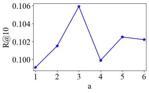
(a) $\mathop{\mathtt{Sci}}\limits$

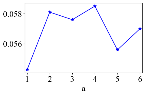
(b) $\mathop{\mathtt{Pantry}}\limits$

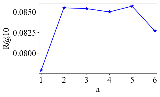
(c) $\mathop{\mathtt{Toys}}\limits$

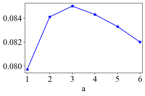
(d) $\mathop{\mathtt{Ins}}\limits$

Figure 3: Recommendation performance of $\mathop{\mathtt{SSNA}}\limits$ over the number of layers to adapt (i.e., $a$)

We conduct a parameter study to evaluate how recommendation performance changes over the number of top LLM layers to be adapted in $\mathop{\mathtt{SSNA}}\limits$ (i.e., $a$). Particularly, we utilize the widely used $\mathop{\mathtt{Sci}}\limits$, $\mathop{\mathtt{Pantry}}\limits$, $\mathop{\mathtt{Toys}}\limits$ and $\mathop{\mathtt{Ins}}\limits$ datasets for this study. On each dataset, we change $a$ while fixing all the other hyper-parameters as the ones reported in Table S1 (Appendix). Figure 3 shows the performance at $\mathop{\mathtt{R@10}}\limits$ on the four datasets.

As shown in Figure 3, on all the four datasets, adapting multiple layers ($a\geq 2$) consistently outperforms that of adapting only the top layer of LLMs ($a=1$). These results demonstrate the effectiveness of jointly adapting the top-$a$ layers ($a\geq 2$) in $\mathop{\mathtt{SSNA}}\limits$. It is also worth noting that, as shown in Figure 3, adapting all the LLM layers ($a=6$) may not benefit the recommendation performance. In fact, on all the datasets, $\mathop{\mathtt{SSNA}}\limits$ achieves the best performance when $a<6$. A possible reason could be that recommendation datasets are generally sparse. Adapting all the LLM layers on sparse recommendation datasets could induce overfitting, and thus, degrade the recommendation performance.

Conclusion

In this paper, we present a novel LLM adaptation method $\mathop{\mathtt{SSNA}}\limits$ for LLM-enhanced SR. $\mathop{\mathtt{SSNA}}\limits$ allows efficient adaptation by learning adapters separate from LLMs and fixing all the pre-trained parameters within LLMs to avoid forward and backward propagation across LLMs in training. $\mathop{\mathtt{SSNA}}\limits$ also enables effective adaptation by jointly adapting the top-$a$ layers of LLMs, and integrating adapters sequentially. We evaluate $\mathop{\mathtt{SSNA}}\limits$ against five state-of-the-art baseline methods on five benchmark datasets using three different LLMs. The experimental results demonstrate that $\mathop{\mathtt{SSNA}}\limits$ substantially outperforms all the baseline methods in terms of recommendation performance, and achieves remarkable improvement in terms of run-time and memory efficiency in training when compared to the best-performing baseline methods $\mathop{\mathtt{LoRA}}\limits$ and $\mathop{\mathtt{ADA}}\limits$ (e.g., 30.8x average speedup over $\mathop{\mathtt{LoRA}}\limits$ across the five datasets). Our analysis also shows the effectiveness of integrating adapters sequentially in $\mathop{\mathtt{SSNA}}\limits$. Our parameter study suggests that adapting top-$a$ layers ($a\geq 2$) of LLMs together in $\mathop{\mathtt{SSNA}}\limits$ substantially benefits the recommendation performance. Our parameters study also shows that adapting all LLM layers for SR tasks may not benefit the recommendation performance.

Appendix

Appendix S1 Best-performing Hyper-parameters

Table S1, Table S2 and Table S3 shows the best-performing hyper-parameters of $\mathop{\mathtt{SSNA}}\limits$ and all the baseline methods when using $\mathop{\mathtt{DistilBERT}}\limits$, $\mathop{\mathtt{DistilRoBERTa}}\limits$ and $\mathop{\mathtt{BERTMedium}}\limits$, respectively.

Table S1: Best-performing Hyper-parameters ($\mathop{\mathtt{DistilBERT}}\limits$)

Dataset	$\mathop{\mathtt{LoRA}}\limits$		$\mathop{\mathtt{ADA}}\limits$		$\mathop{\mathtt{Full}}\limits$		$\mathop{\mathtt{TMLP}}\limits$			$\mathop{\mathtt{TMoE}}\limits$		$\mathop{\mathtt{SSNA}}\limits$
	$p$		$p$		$n_{t}$		$b$	$n_{l}$		$b$		$b$	$a$
$\mathop{\mathtt{Sci}}\limits$	0.1		0.2		2		256	3		128		256	3
$\mathop{\mathtt{Pantry}}\limits$	0.3		0.1		2		256	2		128		256	2
$\mathop{\mathtt{Tools}}\limits$	0.1		0.2		2		256	3		256		256	3
$\mathop{\mathtt{Toys}}\limits$	0.3		0.3		2		256	3		256		256	2
$\mathop{\mathtt{Ins}}\limits$	0.3		0.3		4		256	2		256		256	2

• This table shows the best-performing hyper-parameters of $\mathop{\mathtt{SSNA}}\limits$ and all the baseline methods on the five datasets when using $\mathop{\mathtt{DistilBERT}}\limits$.

Table S2: Best-performing Hyper-parameters ($\mathop{\mathtt{DistilRoBERTa}}\limits$)

Dataset	$\mathop{\mathtt{LoRA}}\limits$		$\mathop{\mathtt{ADA}}\limits$		$\mathop{\mathtt{Full}}\limits$		$\mathop{\mathtt{TMLP}}\limits$			$\mathop{\mathtt{TMoE}}\limits$		$\mathop{\mathtt{SSNA}}\limits$
	$p$		$p$		$n_{t}$		$b$	$n_{l}$		$b$		$b$	$a$
$\mathop{\mathtt{Sci}}\limits$	0.2		0.3		2		256	3		128		64	3
$\mathop{\mathtt{Pantry}}\limits$	0.3		0.2		2		256	1		256		256	2
$\mathop{\mathtt{Tools}}\limits$	0.1		0.2		2		128	3		64		256	3
$\mathop{\mathtt{Toys}}\limits$	0.3		0.3		2		256	3		256		256	2
$\mathop{\mathtt{Ins}}\limits$	0.3		0.3		2		256	2		256		256	2

• This table shows the best-performing hyper-parameters of $\mathop{\mathtt{SSNA}}\limits$ and all the baseline methods on the five datasets when using $\mathop{\mathtt{DistilRoBERTa}}\limits$.

Table S3: Best-performing Hyper-parameters ($\mathop{\mathtt{BERTMedium}}\limits$)

Dataset	$\mathop{\mathtt{LoRA}}\limits$		$\mathop{\mathtt{ADA}}\limits$		$\mathop{\mathtt{Full}}\limits$		$\mathop{\mathtt{TMLP}}\limits$			$\mathop{\mathtt{TMoE}}\limits$		$\mathop{\mathtt{SSNA}}\limits$
	$p$		$p$		$n_{t}$		$b$	$n_{l}$		$b$		$b$	$a$
$\mathop{\mathtt{Sci}}\limits$	0.2		0.1		2		256	3		64		256	2
$\mathop{\mathtt{Pantry}}\limits$	0.2		0.1		2		256	3		256		256	2
$\mathop{\mathtt{Tools}}\limits$	0.2		0.1		2		256	3		64		256	3
$\mathop{\mathtt{Toys}}\limits$	0.3		0.3		2		256	3		256		256	2
$\mathop{\mathtt{Ins}}\limits$	0.3		0.3		4		256	3		256		256	2

• This table shows the best-performing hyper-parameters of $\mathop{\mathtt{SSNA}}\limits$ and all the baseline methods on the five datasets when using $\mathop{\mathtt{BERTMedium}}\limits$.

References

- Bhattacharyya (2022) Bhattacharyya, M. 2022. Gradient Accumulation: Overcoming Memory Constraints in Deep Learning. https://towardsdatascience.com/gradient-accumulation-overcoming-memory-constraints-in-deep-learning-36d411252d01.
- Chen et al. (2022) Chen, Z.; Deng, Y.; Wu, Y.; Gu, Q.; and Li, Y. 2022. Towards understanding mixture of experts in deep learning. arXiv preprint arXiv:2208.02813.
- Devlin et al. (2018) Devlin, J.; Chang, M.-W.; Lee, K.; and Toutanova, K. 2018. Bert: Pre-training of deep bidirectional transformers for language understanding. arXiv preprint arXiv:1810.04805.
- Fan et al. (2022) Fan, Z.; Liu, Z.; Wang, Y.; Wang, A.; Nazari, Z.; Zheng, L.; Peng, H.; and Yu, P. S. 2022. Sequential recommendation via stochastic self-attention. In Proceedings of the ACM Web Conference 2022, 2036–2047.
- He et al. (2021) He, J.; Zhou, C.; Ma, X.; Berg-Kirkpatrick, T.; and Neubig, G. 2021. Towards a unified view of parameter-efficient transfer learning. arXiv preprint arXiv:2110.04366.
- He et al. (2016) He, K.; Zhang, X.; Ren, S.; and Sun, J. 2016. Deep residual learning for image recognition. In Proceedings of the IEEE conference on computer vision and pattern recognition, 770–778.
- He and McAuley (2016) He, R.; and McAuley, J. 2016. Ups and downs: Modeling the visual evolution of fashion trends with one-class collaborative filtering. In proceedings of the 25th international conference on world wide web, 507–517.
- Hidasi et al. (2015) Hidasi, B.; Karatzoglou, A.; Baltrunas, L.; and Tikk, D. 2015. Session-based recommendations with recurrent neural networks. arXiv preprint arXiv:1511.06939.
- Hou et al. (2022) Hou, Y.; Mu, S.; Zhao, W. X.; Li, Y.; Ding, B.; and Wen, J.-R. 2022. Towards universal sequence representation learning for recommender systems. In Proceedings of the 28th ACM SIGKDD Conference on Knowledge Discovery and Data Mining, 585–593.
- Hu et al. (2021) Hu, E. J.; Shen, Y.; Wallis, P.; Allen-Zhu, Z.; Li, Y.; Wang, S.; Wang, L.; and Chen, W. 2021. Lora: Low-rank adaptation of large language models. arXiv preprint arXiv:2106.09685.
- Huang et al. (2021) Huang, J.; Tang, D.; Zhong, W.; Lu, S.; Shou, L.; Gong, M.; Jiang, D.; and Duan, N. 2021. Whiteningbert: An easy unsupervised sentence embedding approach. arXiv preprint arXiv:2104.01767.
- Kang and McAuley (2018) Kang, W.-C.; and McAuley, J. 2018. Self-attentive sequential recommendation. In 2018 IEEE international conference on data mining (ICDM), 197–206. IEEE.
- Liao, Tan, and Monz (2023) Liao, B.; Tan, S.; and Monz, C. 2023. Make Your Pre-trained Model Reversible: From Parameter to Memory Efficient Fine-Tuning. arXiv preprint arXiv:2306.00477.
- Liu et al. (2019) Liu, Y.; Ott, M.; Goyal, N.; Du, J.; Joshi, M.; Chen, D.; Levy, O.; Lewis, M.; Zettlemoyer, L.; and Stoyanov, V. 2019. Roberta: A robustly optimized bert pretraining approach. arXiv preprint arXiv:1907.11692.
- Ma, Kang, and Liu (2019) Ma, C.; Kang, P.; and Liu, X. 2019. Hierarchical gating networks for sequential recommendation. In Proceedings of the 25th ACM SIGKDD international conference on knowledge discovery & data mining, 825–833.
- Mangrulkar et al. (2022) Mangrulkar, S.; Gugger, S.; Debut, L.; Belkada, Y.; and Paul, S. 2022. PEFT: State-of-the-art Parameter-Efficient Fine-Tuning methods. https://github.com/huggingface/peft.
- OpenAI (2023) OpenAI. 2023. GPT-4 Technical Report. ArXiv, abs/2303.08774.
- Peng et al. (2021) Peng, B.; Ren, Z.; Parthasarathy, S.; and Ning, X. 2021. HAM: Hybrid Associations Models for Sequential Recommendation. IEEE Transactions on Knowledge and Data Engineering, 34(10): 4838–4853.
- Sanh et al. (2019) Sanh, V.; Debut, L.; Chaumond, J.; and Wolf, T. 2019. DistilBERT, a distilled version of BERT: smaller, faster, cheaper and lighter. arXiv preprint arXiv:1910.01108.
- Shazeer et al. (2017) Shazeer, N.; Mirhoseini, A.; Maziarz, K.; Davis, A.; Le, Q.; Hinton, G.; and Dean, J. 2017. Outrageously large neural networks: The sparsely-gated mixture-of-experts layer. arXiv preprint arXiv:1701.06538.
- Shim, Choi, and Sung (2021) Shim, K.; Choi, J.; and Sung, W. 2021. Understanding the role of self attention for efficient speech recognition. In International Conference on Learning Representations.
- Tang and Wang (2018) Tang, J.; and Wang, K. 2018. Personalized top-n sequential recommendation via convolutional sequence embedding. In Proceedings of the eleventh ACM international conference on web search and data mining, 565–573.
- Turc et al. (2019) Turc, I.; Chang, M.-W.; Lee, K.; and Toutanova, K. 2019. Well-read students learn better: On the importance of pre-training compact models. arXiv preprint arXiv:1908.08962.
- Vaswani et al. (2017) Vaswani, A.; Shazeer, N.; Parmar, N.; Uszkoreit, J.; Jones, L.; Gomez, A. N.; Kaiser, Ł.; and Polosukhin, I. 2017. Attention is all you need. Advances in neural information processing systems, 30.
- Wang et al. (2022) Wang, J.; Yuan, F.; Cheng, M.; Jose, J. M.; Yu, C.; Kong, B.; He, X.; Wang, Z.; Hu, B.; and Li, Z. 2022. TransRec: Learning Transferable Recommendation from Mixture-of-Modality Feedback. arXiv preprint arXiv:2206.06190.
- Wolf et al. (2020) Wolf, T.; Debut, L.; Sanh, V.; Chaumond, J.; Delangue, C.; Moi, A.; Cistac, P.; Rault, T.; Louf, R.; Funtowicz, M.; Davison, J.; Shleifer, S.; von Platen, P.; Ma, C.; Jernite, Y.; Plu, J.; Xu, C.; Scao, T. L.; Gugger, S.; Drame, M.; Lhoest, Q.; and Rush, A. M. 2020. Transformers: State-of-the-Art Natural Language Processing. In Proceedings of the 2020 Conference on Empirical Methods in Natural Language Processing: System Demonstrations, 38–45. Online: Association for Computational Linguistics.
- Yuan et al. (2023) Yuan, Z.; Yuan, F.; Song, Y.; Li, Y.; Fu, J.; Yang, F.; Pan, Y.; and Ni, Y. 2023. Where to go next for recommender systems? id-vs. modality-based recommender models revisited. arXiv preprint arXiv:2303.13835.
- Zaken, Ravfogel, and Goldberg (2021) Zaken, E. B.; Ravfogel, S.; and Goldberg, Y. 2021. Bitfit: Simple parameter-efficient fine-tuning for transformer-based masked language-models. arXiv preprint arXiv:2106.10199.
- Zhang et al. (2023) Zhang, Q.; Chen, M.; Bukharin, A.; He, P.; Cheng, Y.; Chen, W.; and Zhao, T. 2023. Adaptive budget allocation for parameter-efficient fine-tuning. arXiv preprint arXiv:2303.10512.