Angular Correlations of Cosmic Microwave Background Spectrum Distortions from Photon Diffusion

Abstract

During cosmic recombination, charged particles bind into neutral atoms and the mean free path of photons rapidly increases, resulting in the familiar diffusion damping of primordial radiation temperature variations. An additional effect is a small photon spectrum distortion, because photons arriving from a particular sky direction were originally in thermal equilibrium at various spatial locations with different temperatures; the combination of these different blackbody temperature distributions results in a spectrum with a Compton $y$-distortion. Using the approximation that photons had zero mean free path prior to their second-to-last scattering, we derive an expression for the resulting $y$-distortion, and compute the angular correlation function of the diffusion $y$-distortion and its cross-correlation with the square of the photon temperature fluctuation. Detection of the cross-correlation is within reach of existing arcminute-resolution microwave background experiments such as the Atacama Cosmology Telescope and the South Pole Telescope.

1 Introduction

The average of two or more blackbody spectra at different temperatures is not a perfect blackbody. The Cosmic Microwave Background (CMB) photons arriving from a particular line of sight (LOS) scattered multiple times during recombination before their last-scattering into that LOS. Because CMB photons at the epoch of last scattering have energies that are far smaller than the electron rest mass, the fractional energy change of a scattered photon is small (of order $E_{\gamma}/m_{e}c^{2}$ by the Klein-Nishina formula (Klein & Nishina, 1929, as translated in Klein & Nishina (1994)). Therefore, to a good approximation, photon last-scattering does not change the photon’s energy but only its propagation direction.

If the photons of the CMB came to us along each LOS unscattered from a “surface of last thermal emission,” then they would be drawn from the thermal-equilibrium blackbody distribution in their local neighborhood of emission. Instead, the CMB photons are scattered with nearly no change in energy into the LOS at their point of last scattering. The photon energies are therefore drawn, approximately, from the black-body distributions of the neighborhoods from which the photons originated. The energy distribution of the photons arriving along each LOS is approximately the average of many blackbodies, each with the temperature of a different neighborhood of photon emission.

A simple approximation to this averaging effect is to assume that each CMB photon scatters exactly once after its emission from a blackbody, or equivalently that the photon mean-free-path is negligible prior to its second-to-last scattering (2LS). We therefore take the point of emission, whose temperature distribution the photon samples, to be the point of second-last scattering. In this approximation, we provide an analytic expression for the contribution of any given Fourier mode of adiabatic perturbation to the photon spectrum from a given sky direction. The net effect of all such perturbation modes is an integral over the contribution of each mode, which can be evaluated numerically. The first-order effect (in the difference between the temperatures in the second-last-scattering neighborhood and the global average temperature at that cosmic time) is a blackbody photon distribution with a temperature averaged over the region of second-to-last scatterings; this averaging approximates the mechanism behind the familiar diffusion damping of temperature anisotropies on small angular scales. The second-order effect is a $y$-distortion of the blackbody distribution first described (but not quantified) in (Zel’dovich et al., 1972), and recalled in (Chluba & Sunyaev, 2004). More details were provided in (Khatri et al., 2012), but again without specific predictions. A calculation of the mean expected distortion may be among the effects included in (Chluba et al., 2012). Similarly, it is described in (Sunyaev & Khatri, 2013; Chluba, 2016).

We calculate this effect, showing that the $y$-distortion angular correlation function is at a level that is potentially measurable in future experiments, but confirm that it is small compared to other expected signals (Chluba & Sunyaev, 2004). We also calculate the angular cross-correlation function of this y-distortion and the square of the temperature fluctuations. The cross-correlation is likely detectable in current experiments, including the Atacama Cosmology Telescope (ACT) (Coulton et al., 2023) and the South Pole Telescope (SPT) (Bleem et al., 2022), and especially in anticipated experiments like the Simons Observatory (Galitzki et al., 2018) and CMB-S4 (Abitbol et al., 2017b). The authors of (Chluba et al., 2022) and (Kite et al., 2022) address related questions, including cross-correlations, although not specifically this effect.

The mixing of blackbody photon distributions is distinct from the averaging of temperatures over different lines of sight, whether through the finite width of telescope beams (e.g. Chluba & Sunyaev, 2004) or through the angular integration inherent in the calculation of the coefficients of spherical harmonics (e.g. Lucca et al., 2020). Each of these effects also creates small $y$-distortions in measured signals through temperature averaging, but the effect discussed here is due to physical processes during the epoch of last scattering and thus carries information about the universe rather than about a given measurement.

In §​ 2, we calculate the distribution of second-last-scattering locations. In §​ 3, we calculate the expected $y$-distortion $\mathcal{Y}$ of the CMB spectrum due to this diffusive averaging. In §​ 4, we calculate the expected angular correlation function of $\mathcal{Y}$, as well as the expected cross-correlation between $\mathcal{Y}$ and the square of the observed temperature fluctuation $({\Delta T})^{2}$. We discuss the detectability of this signal in §​ 5, and conclude in §​ 6.

2 Second-to-Last Scattering Distribution

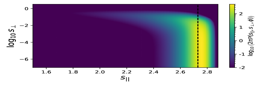
Figure 1: $\mathcal{P}(s_{||},s_{\perp},\phi=0)$ over a range of $s_{||},s_{\perp}$, colored by $\log_{10}\!\left(2\pi\mathcal{P}\right)$. $\mathcal{P}$ peaks at $s_{||}\simeq 2.76$ – just slightly higher than $s_{\rm recombination}=2.73$ (dashed line) – and at $s_{\perp}\lesssim 10^{-3}$ (below which it is approximately constant). When sampling from $\mathcal{P}$ each decade in $s_{\perp}$ contributes approximately one-tenth the samples as the previous decade; thus we display only $s_{\perp}\geq 10^{-7}$. The other boundaries of the domain of $\mathcal{P}$ are taken at sufficient distance from the higher probability regions of $\mathcal{P}$ that enlarging the domain does not impact the results.

Photons arriving at a common point of last scattering $\mathbf{x_{1}}$ come from a surrounding neighborhood of prior locations $\mathbf{x_{2}}$, where we use the subscript to label the scattering number, counting back in time from observation at scattering “0”. Arriving at $\mathbf{x_{1}}$, the photons scatter into the LOS and their combined distribution is no longer that of a perfect blackbody; it is an average of blackbodies. The resulting distortion of the blackbody spectrum retains information about the distribution of temperatures in the second-last-scattering neighborhood that goes beyond the intensity of the photon emissions from that LOS.

To calculate the observational effects of this blackbody averaging, we must first calculate the probability density $\mathcal{P}(\mathbf{x_{2}},\mathbf{x_{1}})$ that a photon arriving at the observer from a last-scattering location $\mathbf{x_{1}}$ had its second-last scattering at $\mathbf{x_{2}}$. While we refer to our location as “the observer,” in order to remove the physically distinct effects of propagation through the low-redshift universe, we consider a reference point $\mathbf{x_{0}}$ at co-moving distance $r_{0}$ from us along the LOS, which is the line between the observer and $\mathbf{x_{1}}$. We take $\mathbf{x_{0}}$ to be at a redshift $z_{0}=100$, well after recombination and last scattering (at $z\simeq 10^{3}$) but well before the onset of cosmic acceleration. The comoving displacement of the j-th-last scatter from the i-th-last-scattering location is $\mathbf{x_{ij}}\equiv\mathbf{x_{j}}-\mathbf{x_{i}}$. We also write $r_{ij}$ for $\lvert\mathbf{x_{ij}}\rvert$.

To leading order (in fluctuations around the homogeneous background metric and stress-energy tensor), the probability distribution $\mathcal{P}(\mathbf{x_{2}},\mathbf{x_{1}})$ is rotationally symmetric about the line-of-sight axis. $\mathcal{P}(\mathbf{x_{2}},\mathbf{x_{1}})$ can thus be written in terms of:

1. $P_{1}(r_{01})\,\mathrm{d}{r_{01}}$, the probability that last scattering occurs at a comoving distance from $\mathbf{x_{0}}$ between $r_{01}$ and $r_{01}+\mathrm{d}{r_{01}}$ along the LOS

   $$P_{1}(r_{01})=\overline{g_{\gamma}}(r_{0}+r_{01},r_{0})\,,$$ (1)

   where $\overline{g_{\gamma}}(r_{a},r_{b})$ is the visibility function for Compton scattering between comoving radii $r_{a}$ and $r_{b}\geq r_{a}$ (see Appendix Appendix B);

2. $P_{\theta}(\theta)\,\mathrm{d}{\theta}$, the probability that the last scattering is through an angle between $\theta$ and $\theta+\mathrm{d}{\theta}$

   $$P_{\theta}(\theta)=\frac{\mathrm{d}{\sigma_{T}}}{\mathrm{d}{\theta}}=\frac{3}{8}\sin\theta\left(1+\cos^{2}\theta\right)\,\,,\ \theta\in[0,\pi]\,;$$ (2)

3. $P_{\phi}(\phi)$, the probability distribution of the last scattering azimuth

   $$P_{\phi}(\phi)=\frac{1}{2\pi}\,\,,\ \phi\in[0,2\pi)\,;$$ (3)

4. $P_{2}(r_{12}|r_{01})\,dr_{12}$, the probability of the 2nd-to-last scatter taking place at a comoving distance between $r_{12}$ and $r_{12}+dr_{12}$ from the last scattering at comoving distance $r_{01}$ from $\mathbf{x_{0}}$

   $$P_{2}(r_{12}|r_{01})=\overline{g_{\gamma}}(r_{0}+r_{01}+r_{12},r_{0}+r_{01})\,.$$ (4)

The overbar on $\overline{g_{\gamma}}$ in eq. 1 and 4 indicates that we are considering $\overline{g_{\gamma}}$ to be a function only of redshift, i.e. a homogeneous function of location on a given redshift slice. The arguments of $\overline{g_{\gamma}}$ are cosmological epochs, not positions; thus in eq. 4, $r_{01}+r_{12}\neq r_{02}$. From eq. 1, it is clear that $\overline{g_{\gamma}}(r_{a},r_{b})$ is normalized such that $\int\mathrm{d}{r_{a}}\overline{g_{\gamma}}(r_{a},r_{b})=1$. We note that $P_{2}$ is independent of scattering angle $\theta$ (to leading order).

Multiplying these four probabilities – $P_{1}$, $P_{\theta}$, $P_{\phi}$, and $P_{2}$ – gives the probability density $\mathcal{P}$ for the last scattering to take place at comoving distance $r_{01}$ from the observer and the second-last scattering to take place at comoving distance $r_{12}$ from the last scattering, with scattering angle $\theta$ and azimuthal angle $\phi$.

We prefer to express $\mathcal{P}$ in terms of new dimensionless comoving coordinates $s_{||}$ and $s_{\perp}$ measured respectively along the LOS (in the ${\bf\hat{n}}$ direction) and perpendicular to it, instead of $r_{12}$ and $\theta$.Thus

$$\mathbf{x}(\mathbf{s};{\bf\hat{n}})=r_{0}{\bf\hat{n}}+L_{\rm eq}\mathbf{s}\,,$$ (5)

where $L_{\rm eq}$ is defined in Appendix Appendix A. We define the vector $\mathbf{s}$, with origin at $\mathbf{r_{0}}$, i.e. along the LOS at redshift $z_{0}$. $\mathbf{s}$ is directed away from the reference point and away from the observer; it can be decomposed as

$$\mathbf{s}=s_{||}{\bf\hat{n}}+\mathbf{s}_{\perp}\,.$$ (6)

$\mathbf{s}_{\perp}$ is a two-vector of magnitude $s_{\perp}$ in the plane perpendicular to ${\bf\hat{n}}$. The direction of $\mathbf{s}_{\perp}$ is specified by $\phi$.

$$s_{||}=\frac{r_{01}}{L_{\rm eq}}+\frac{r_{12}}{L_{\rm eq}}\cos\theta\quad\mathrm{and}\quad s_{\perp}=\frac{r_{12}}{L_{\rm eq}}\sin\theta.$$ (7)

We can take the new set of variables to be $r_{01}$, $s_{\perp}$, $s_{||}$, and $\phi$, leading to a Jacobian factor

$$J=\frac{L_{\rm eq}^{3}}{r_{12}}=\frac{L_{\rm eq}^{3}}{\left((L_{\rm eq}s_{||}-r_{01})^{2}+L_{\rm eq}^{2}s_{\perp}^{2}\right)^{1/2}}\,.$$ (8)

In terms of these new variables

$$\mathcal{P}_{\theta}(\theta)=\left(\frac{3L_{\rm eq}s_{\perp}}{8}\right)\frac{2(L_{\rm eq}s_{||}-r_{01})^{2}+L_{\rm eq}^{2}s_{\perp}^{2}}{\left((L_{\rm eq}s_{||}-r_{01})^{2}+L_{\rm eq}^{2}s_{\perp}^{2}\right)^{3/2}}$$ (9)

The probability density $\mathcal{P}(s_{||},s_{\perp},\phi)$ is then

$$\mathcal{P}(s_{||}, s_{\perp},\phi)=\int\!\!\!\mathrm{d}{r_{01}}\;\mathcal{P}(r_{01},r_{12},\theta,\phi)J=\int\!\!\!\mathrm{d}{r_{01}}\;P_{2}(r_{12}|r_{01})\,P_{1}(r_{01})\,P_{\theta}(\theta)\,P_{\phi}(\phi)\,J$$ (10)

$$=\frac{L_{\rm eq}^{2}}{2\pi}\!\!\int\!\!\!\mathrm{d}{r_{01}}\;\overline{g_{\gamma}}(r_{0}+r_{01},r_{0})\,\overline{g_{\gamma}}\left(r_{0}+r_{01}+\sqrt{(L_{\rm eq}s_{||}-r_{0}+r_{01})^{2}+L_{\rm eq}^{2}s_{\perp}^{2}},r_{0}+r_{01}\right)\left(\frac{3L_{\rm eq}s_{\perp}}{8}\right)\frac{2(L_{\rm eq}s_{||}-r_{01})^{2}+L_{\rm eq}^{2}s_{\perp}^{2}}{\left((L_{\rm eq}s_{||}-r_{01})^{2}+L_{\rm eq}^{2}s_{\perp}^{2}\right)^{2}}\,.$$ (11)

The numerical evaluation of $\mathcal{P}(s_{||},s_{\perp},\phi)$ is described in Appendix Appendix C, and the result is presented in Fig. 1. We observe that $\mathcal{P}$ is sharply peaked close to the position of recombination, i.e at $s_{||}\simeq s_{\rm recombination}$, and with $s_{\perp}\lesssim 10^{-3}$.

3 Calculating the Signal

Consider a sum of blackbodies, each with photon occupation number $n_{Pl}(\chi)=(e^{\chi}-1)^{-1}$ for $\chi\equiv h\nu/kT_{i}$. To third order in the temperature fluctuations $\epsilon_{i}\equiv\dfrac{T_{i}-\bar{T}}{\bar{T}}$:

$$\sum_{i} a_{i}n_{Pl}(\chi,\!T_{i})=n_{Pl}(\chi,\bar{T})\!\!\sum_{i}\!a_{i}+n_{Pl}^{2}(\chi,\bar{T})\chi e^{\chi}\!\sum_{i}\!a_{i}\epsilon_{i}$$ (12)

$$\phantom{=}+\frac{1}{2}n_{Pl}^{3}(\chi,\bar{T})\left((\chi^{2}\!\!-\!2\chi)e^{2\chi}\!+\!(\chi^{2}\!\!+\!2\chi)e^{\chi}\right)\!\sum_{i}\!a_{i}\epsilon_{i}^{2}+\mathcal{O}(\epsilon_{i}^{3})$$

We can choose to normalize $a_{i}$ so that $\sum_{i}a_{i}=1$. Taking $\bar{T}\equiv\sum_{i}a_{i}T_{i}$ as one would expect, then $\sum_{i}a_{i}\epsilon_{i}=0$.

It is conventional and convenient to reorganize eq. 12, writing:

$$\sum_{i}a_{i}n_{Pl}(\chi,\!T_{i}) =n_{Pl}(\chi,\hat{T})+\left[\sum_{i}\!a_{i}(\delta_{i}-\delta_{i}^{2})\right]n_{Pl}^{2}(\chi,\hat{T})\chi e^{\chi}$$

$$\!\!\!\!\!\!\!\!\!\!+\frac{1}{2}\!\left[\sum_{i}\!a_{i}\delta_{i}^{2}\right]n_{Pl}^{3}(\nu,\hat{T})\chi^{2}e^{\chi}(e^{\chi}+1)+\mathcal{O}(\delta^{3})$$ (13)

where

$$\delta_{i}\equiv\frac{T_{i}-\hat{T}}{\hat{T}}.$$ (14)

We are free to choose $\hat{T}$ and do so such that

$$\sum_{i}a_{i}(\delta_{i}-\delta_{i}^{2})=0\,.$$ (15)

This choice of $\hat{T}$ means §​ 3 is a pure $y$-distortion:

$$\sum_{i}a_{i} n_{Pl}(\chi,T_{i})=n_{Pl}(\chi,\hat{T})$$ (16)

$$\phantom{=}+\frac{1}{2}\left[\sum_{i}a_{i}\delta_{i}^{2}\right]n_{Pl}^{3}(\chi,\hat{T})\chi^{2}e^{\chi}(e^{\chi}+1)+\mathcal{O}(\delta^{3})\,.$$

Clearly $\hat{T}\neq\bar{T}$, but how different are they, or more importantly how different are $\bar{\delta^{2}}\equiv\sum_{i}a_{i}\delta_{i}^{2}$ and $\bar{\epsilon^{2}}\equiv\sum_{i}a_{i}\epsilon_{i}^{2}$? We can solve the quadratic eq. 15 for $\hat{T}$ and expand $\hat{T}$ around $\bar{T}$ to find

$$\hat{T}=\bar{T}\left[1-\frac{1}{2}\bar{\epsilon^{2}}+{\cal{O}}(\bar{\epsilon}^{4})\right]\,.$$ (17)

It is straightforward to show that

$$\delta_{i}=\epsilon_{i}-(1+\epsilon_{i})\bar{\epsilon^{2}}+{\cal{O}}(\epsilon^{4})\,.$$ (18)

and thus

$$\sum_{i}a_{i}\delta_{i}^{2}=\sum_{i}a_{i}\epsilon_{i}^{2}+{\cal{O}}(\epsilon^{4})\,.$$ (19)

For small fluctuations, we can therefore replace $\hat{T}$ by $\bar{T}$, and $\delta_{i}$ by $\epsilon_{i}$ in the calculation of the signal, which proves considerably simpler.

In the CMB, photons were scattered into the LOS at last-scattering from different locations of second-last scattering. We take the photon distribution originating from each 2LS point to be a blackbody of the temperature characteristic of the plasma there. In this approximation, the resulting observable photon distribution is the weighted average of the 2LS blackbodies at all the accessible 2LS points. We must therefore account for the temperature at each location $\mathbf{x}(\mathbf{s},{\bf\hat{n}})$ that can scatter into the LOS, and we must weight the sum by the probability $\mathcal{P}(\mathbf{s})$ that the photons we see come from that location.

The temperature at $\mathbf{x}(\mathbf{s},{\bf\hat{n}})$ is given by

$$T(\mathbf{x}(\mathbf{s},{\bf\hat{n}})) =T_{0}+\int\!\!\!\mathrm{d}^{3}{\!k}\,A^{\!\mathcal{T}\!\!}(\mathbf{k})\,e^{i\mathbf{k}\cdot\mathbf{x}(\mathbf{s},{\bf\hat{n}})}$$ (20)

$$\equiv T_{0}+{\Delta T}(\mathbf{x}(\mathbf{s},{\bf\hat{n}}))\,,$$

where $T_{0}$ is the mean CMB temperature. $A^{\!\mathcal{T}\!\!}(\mathbf{k})$ includes the effect of the transfer function $\mathcal{T}(\lvert\mathbf{k}\rvert)$ on the primordial amplitude $A(\mathbf{k})$ of the Fourier mode of the primordial curvature fluctuation with wave vector $\mathbf{k}$:

$$A^{\!\mathcal{T}\!\!}(\mathbf{k})\equiv\mathcal{T}(\lvert\mathbf{k}\rvert)A(\mathbf{k})\,.$$ (21)

The appropriate weighted mean temperature of the photons scattered into the LOS in direction ${\bf\hat{n}}$ is

$$\bar{T}({\bf\hat{n}}) =\int\!\!\!\mathrm{d}^{3}{\!s}\,\mathcal{P}(\mathbf{s})\,\left(T_{0}+\int\mathrm{d}^{3}{\!k}A^{\!\mathcal{T}}(\mathbf{k})e^{i\mathbf{k}\cdot\mathbf{x}(\mathbf{s},{\bf\hat{n}})}\right)$$ (22)

$$=T_{0}+\Delta\bar{T}({\bf\hat{n}})\,.$$ (23)

The $y$-distortion signal is

$$\mathcal{Y}({\bf\hat{n}}) =\frac{1}{2}\int\!\!\!\mathrm{d}{\mathbf{s}}\;\mathcal{P}(\mathbf{s})\left(\frac{T(\mathbf{x}(\mathbf{s};{\bf\hat{n}}))-\bar{T}({\bf\hat{n}})}{\bar{T}({\bf\hat{n}})}\right)^{2}$$ (24)

$$\simeq\frac{1}{2T_{0}^{2}}\int\!\!\!\mathrm{d}{\mathbf{s}}\;\mathcal{P}(\mathbf{s})\left({\Delta T}(\mathbf{x}(\mathbf{s};{\bf\hat{n}}))-\Delta\bar{T}({\bf\hat{n}})\right)^{2}$$ (25)

$$=\frac{1}{2T_{0}^{2}}\bigg{[}\int\!\!\!\mathrm{d}{\mathbf{s}}\;\mathcal{P}(\mathbf{s})\left({\Delta T}(\mathbf{x}(\mathbf{s};\mathbf{{\bf\hat{n}}}))\right)^{2}$$ (26)

$$\qquad-\int\!\!\!\mathrm{d}{\mathbf{s}_{1}}\mathrm{d}{\mathbf{s}_{2}}\;\mathcal{P}(\mathbf{s}_{1})\mathcal{P}(\mathbf{s}_{2}){\Delta T}(\mathbf{x}(\mathbf{s}_{1};\mathbf{{\bf\hat{n}}})){\Delta T}(\mathbf{x}(\mathbf{s}_{2};\mathbf{{\bf\hat{n}}}))\bigg{]}\,,$$

where again $\mathrm{d}{\mathbf{s}}\equiv\mathrm{d}{s_{||}}\mathrm{d}{s_{\perp}}\mathrm{d}{\phi_{s}}$.

Expectation values pass through integrals to apply only to the factors of ${\Delta T}$, so that $\left\langle\mathcal{Y}(\mathbf{{\bf\hat{n}}})\right\rangle$ can be expressed in terms of the correlation function $\xi\left(\lvert\mathbf{x}_{2}-\mathbf{x}_{1}\rvert\right)$ of the Gaussian ${\Delta T}$ field:

$$\left\langle\mathcal{Y}(\mathbf{{\bf\hat{n}}})\right\rangle\!=\!\frac{1}{2T_{0}^{2}}\left[\xi(0)\!-\!\!\int\!\!\!\mathrm{d}{\mathbf{s}_{1}}\mathrm{d}{\mathbf{s}_{2}}\mathcal{P}(\mathbf{s}_{1})\mathcal{P}(\mathbf{s}_{2})\xi(L_{\rm eq}\lvert\mathbf{s}_{1}-\mathbf{s}_{2}\rvert)\right],$$ (27)

where we have used the fact that

$$\mathbf{x}(\mathbf{s}_{1};\mathbf{{\bf\hat{n}}})-\mathbf{x}(\mathbf{s}_{2};\mathbf{{\bf\hat{n}}})=L_{\rm eq}\,(\mathbf{s}_{1}-\mathbf{s}_{2})\,.$$ (28)

Unsurprisingly, $\langle\mathcal{Y}\rangle$ is independent of direction, since we have assumed here that $\xi$ is statistically isotropic, at least on the small scales over which diffusion takes place during recombination:

$$\xi(\lvert\mathbf{x}_{2} -\mathbf{x}_{1}\rvert)\equiv\left\langle{\Delta T}(\mathbf{x}_{1}){\Delta T}(\mathbf{x}_{2})\right\rangle$$ (29)

$$=\int\!\!\!\mathrm{d}^{3}{\!k_{1}}\mathrm{d}^{3}{\!k_{2}}\;e^{i(\mathbf{k}_{1}\cdot\mathbf{x}_{1}-\mathbf{k}_{2}\cdot\mathbf{x}_{2})}\langle A^{T}(\mathbf{k}_{1})A^{T*}(\mathbf{k}_{2})\rangle$$ (30)

$$=\int\!\!\!\mathrm{d}^{3}{\!k_{1}}\mathrm{d}^{3}{\!k_{2}}\;e^{i(\mathbf{k}_{1}\cdot\mathbf{x}_{1}-\mathbf{k}_{2}\cdot\mathbf{x}_{2})}\delta^{(3)}(\mathbf{k}_{1}-\mathbf{k}_{2})P^{TT}(\lvert\mathbf{k}_{1}\rvert)$$ (31)

$$=\int\!\!\!\mathrm{d}^{3}{\!k}\;e^{i\mathbf{k}\cdot(\mathbf{x}_{1}-\mathbf{x}_{2})}P^{TT}(\lvert\mathbf{k}\rvert)$$ (32)

The TT power spectrum $P^{TT}$ is the product of the initial power spectrum of the gauge-invariant curvature perturbations times the “early” temperature transfer function squared

$$P^{TT}(\lvert\mathbf{k}\rvert)=\frac{T_{0}^{2}}{4\pi}\frac{A_{S}(k_{\star})}{k^{3}}\left(\frac{k}{k_{\star}}\right)^{n_{s}-1}({\cal{T}}^{e}(k))^{2}e^{-2(k/k_{2\rm{LS}})^{2}}\,.$$ (33)

Here $k_{\star}=0.05h^{-1}\rm{Mpc}$ is an arbitrary, but conventional, pivot scale. The high-k cutoff $k_{2\rm{LS}}$, accounting for the damping up to second-last-scattering, can be written in terms of the conformal-time rate of change of the opacity (Jungman et al., 1996), or more simply read directly from Baumann (2022, eq. 7.139)

$$k_{2\rm{LS}}^{-1}\simeq 8.8\ \rm{Mpc}.$$ (34)

We take the transfer function ${\cal{T}}^{e}(k)$ to be approximately the pure Sachs-Wolfe power spectrum, and, assuming that it changes slowly with time, evaluate it at the time of last scattering, rather than the time of second-last scattering (we use Baumann, 2022, 7.112):

$$\mathcal{T}^{e}(k) \simeq\left.{\mathcal{T}}_{\rm SW}\right|_{\rm LS}(k)$$ (35)

$$\simeq\frac{1}{5}\left[(1+R(z_{\rm LS}))^{-1/4}\cos(kr_{s}(z_{\rm LS}))-3R(z_{\rm LS})\right]$$ (36)

The label $e$ stands for early, i.e. during recombination, as opposed to the usual transfer function ${\cal{T}}^{l}(k)$, evaluated late, i.e. at redshift $z_{0}=100$. Here

$$R(z)\equiv\frac{3}{4}\frac{\Omega_{b}}{\Omega_{\gamma}(1+z)}\simeq 0.6\frac{\Omega_{b}h^{2}}{0.02}\frac{10^{3}}{1+z}$$ (37)

and the sound horizon at emission (see Baumann, 2022, Appendix C) is

$$r_{s}(z_{\rm LS} )=\int_{\infty}^{z_{\rm LS}}c_{s}\frac{\mathrm{d}{\tau}}{\mathrm{d}{z}}\mathrm{d}{z},$$ (38)

$$=\frac{2c(1\!+\!z_{\rm eq})}{3H(z_{\rm eq})}\sqrt{\frac{6}{R_{\rm eq}}}\ln\left(\frac{\sqrt{1+R(z)}+\sqrt{R(z)+R_{\rm eq}}}{1+\sqrt{R_{\rm eq}}}\right)$$ (39)

$$\simeq 144\ \rm{Mpc}\,.$$ (40)

Thus,

$$\xi^{ee}\left(r_{12}\right)$$ (41)

$$\ \simeq\frac{T_{0}^{2}A_{s}(k_{*})}{r_{12}}\!\!\int_{k_{\rm min}}^{\infty}\!\!\frac{\mathrm{d}{k}}{k^{2}}\left(\frac{k}{k_{*}}\right)^{n_{s}-1}\!\!\left(\mathcal{T}^{e}_{\rm{SW}}(k)e^{-\left(\frac{k}{k_{2\rm{LS}}}\right)^{2}}\right)^{2}\sin(kr_{12})\,.$$

The result is independent of the low-$k$ cutoff for $k_{\rm min}\lesssim 1\times 10^{-2}\ \rm{Mpc}^{-1}$.

Using the best current value (Planck Collaboration et al., 2020a) of $A_{s}\simeq 2.1\times 10^{-9}$ gives

$$\langle\mathcal{Y}({\bf\hat{n}})\rangle\simeq 9.1\times 10^{-11}\,.$$ (42)

Since the variance in the (dipole-subtracted) CMB temperature anisotropies,

$$\mathrm{var}(T)\Big{|}_{\mathrm{Planck}}=(15\,\mu\mathrm{K})^{2}\,,$$ (43)

we might have thought that the maximum signal would be

$$\langle\mathcal{Y}({\bf\hat{n}})\rangle|_{\mathrm{expect}}=\frac{1}{2}\left(\frac{15\mu\mathrm{K}}{2.7\mathrm{K}}\right)^{2}\simeq 1.5\times 10^{-11}.$$ (44)

However, the observed CMB fluctuations themselves are damped compared to their amplitude at second-last scattering. Without that damping (i.e. eliminating the exponential term in eq. 41), the signal would have been

$$\langle\mathcal{Y}({\bf\hat{n}})\rangle|_{\mathrm{no-damping}}=2.8\times 10^{-9}$$ (45)

Damping of short range fluctuations is thus responsible for a factor-of-31 suppression in the signal from its maximum possible value.

4 Correlation function of the signal and temperature fluctuations

Unlike the $y$-distortions that arise from the time-evolution of the background physics during recombination, the $y$-distortions due to local blackbody averaging are anisotropic. We are therefore interested in calculating the angular correlation function of $\mathcal{Y}({\bf\hat{n}})$ with the temperature fluctuations themselves ${\Delta T}({\bf\hat{n}}^{\prime})$. The particular form of this cross-correlation is distinctive to the diffusion distortion signal, and can be used to disentangle diffusion distortion from foregrounds.

Since the fluctuations are nearly Gaussian, the expected correlation of $\mathcal{Y}({\bf\hat{n}})$ with ${\Delta T}({\bf\hat{n}}^{\prime})$ is a three-point function, and nearly vanishes. However, the correlation of $\mathcal{Y}({\bf\hat{n}})$ with $({\Delta T}({\bf\hat{n}}^{\prime}))^{2}$ does not:

$$\frac{1}{T_{0}^{2}}\mathcal{Y}({\bf\hat{n}}_{1})({\Delta T}({\bf\hat{n}}_{2}))^{2}$$ (46)

$$\quad=\frac{1}{2T_{0}^{4}}\Bigg{[}\ \phantom{+}\int\!\!\!\mathrm{d}{\mathbf{s}_{1}}\;\mathcal{P}(\mathbf{s}_{1})\left({\Delta T}(\mathbf{x}({\bf\hat{n}}_{1},\mathbf{s}_{1})\right)^{2}$$

$$\qquad\qquad\ -\int\!\!\!\mathrm{d}{\mathbf{s}_{1}}\;\mathcal{P}(\mathbf{s}_{1})\mathrm{d}{\mathbf{s}^{\prime}_{1}}\mathcal{P}(\mathbf{s}^{\prime}_{1}){\Delta T}(\mathbf{x}({\bf\hat{n}}_{1},\mathbf{s}_{1}){\Delta T}(\mathbf{x}({\bf\hat{n}}_{1},\mathbf{s}^{\prime}_{1})\Bigg{]}$$

$$\qquad\quad\times\int\!\!\!\mathrm{d}{\mathbf{s}_{2}}\;\mathcal{P}(\mathbf{s}_{2})\mathrm{d}{\mathbf{s}^{\prime}_{2}}\mathcal{P}(\mathbf{s}^{\prime}_{2}){\Delta T}(\mathbf{x}({\bf\hat{n}}_{2},\mathbf{s}_{2}){\Delta T}(\mathbf{x}({\bf\hat{n}}_{2},\mathbf{s}^{\prime}_{2})$$

so

$$C^{\mathcal{Y}({\Delta T})^{2}}(\mathbf{{\bf\hat{n}}}_{1},\mathbf{{\bf\hat{n}}}_{2})$$

$$\quad\equiv\Big{\langle}\frac{1}{T_{0}^{2}}\mathcal{Y}({\bf\hat{n}}_{1})({\Delta T}({\bf\hat{n}}_{2}))^{2}\Big{\rangle}-\frac{1}{T_{0}^{2}}\Big{\langle}\mathcal{Y}({\bf\hat{n}}_{1})\Big{\rangle}\Big{\langle}({\Delta T}({\bf\hat{n}}_{2}))^{2}\Big{\rangle}$$ (47)

$$\quad=\phantom{+}\frac{1}{T_{0}^{4}}\int\!\!\!\mathrm{d}{\mathbf{s}_{1}}\mathcal{P}(\mathbf{s}_{1})\mathrm{d}{\mathbf{s}_{2}}\mathcal{P}(\mathbf{s}_{2})\mathrm{d}{\mathbf{s}^{\prime}_{2}}\mathcal{P}(\mathbf{s}^{\prime}_{2})$$ (48)

$$\qquad\qquad\xi^{el}\left(\lvert\mathbf{x}({\bf\hat{n}}_{1},\mathbf{s}_{1})-\mathbf{x}({\bf\hat{n}}_{2},\mathbf{s}_{2})\rvert\right)\xi^{el}\left(\lvert\mathbf{x}({\bf\hat{n}}_{1},\mathbf{s}_{1})-\mathbf{x}({\bf\hat{n}}_{2},\mathbf{s}^{\prime}_{2})\rvert\right)$$

$$\qquad-\frac{1}{T_{0}^{4}}\left(\int\!\!\!\mathrm{d}{\mathbf{s}_{1}}\mathcal{P}(\mathbf{s}_{1})\mathrm{d}{\mathbf{s}_{2}}\mathcal{P}(\mathbf{s}_{2})\xi^{el}\left(\lvert\mathbf{x}({\bf\hat{n}}_{1},\mathbf{s}_{1})-\mathbf{x}({\bf\hat{n}}_{2},\mathbf{s}_{2})\rvert\right)\right)^{2}\,.$$

(See Appendix Appendix D for a full derivation.)

Given a statistically isotropic universe, $C^{\mathcal{Y}(\Delta T)^{2}}(\mathbf{{\bf\hat{n}}}_{1},\mathbf{{\bf\hat{n}}}_{2})$ depends only on ${\bf\hat{n}}_{1}\cdot{\bf\hat{n}}_{2}\equiv\cos\theta$. Here

$$\xi^{el}\left(r_{12}\right) \simeq\frac{T_{0}^{2}A_{s}(k_{*})}{r_{12}}\int_{k_{\rm min}}^{\infty}\!\!\frac{\mathrm{d}{k}}{k^{2}}\left(\frac{k}{k_{*}}\right)^{n_{s}-1}\!\!\!\!\!\!\!\!\mathcal{T}^{e}(k)\mathcal{T}^{l}(k)$$ (49)

$$\qquad\qquad\qquad\qquad\qquad\times e^{-2(k/k_{2LS})^{2}}\sin(kr_{12})\,,$$

with ${\cal{T}}^{l}(k)$ obtained by evaluating ${\cal{T}}_{SW}(k)$ from (35) at $z_{0}$.

In the upper panel of Fig. 3, we plot $C^{\mathcal{Y}({\Delta T})^{2}}(\theta)$ in purple and, for comparison (in blue), the pure-SW $({\Delta T})^{2}-({\Delta T})^{2}$ auto-correlation function

$$C {}^{({\Delta T})^{2}({\Delta T})^{2}}(\mathbf{{\bf\hat{n}}}_{1}\cdot\mathbf{{\bf\hat{n}}}_{2})$$

$$\equiv\frac{1}{T_{0}^{4}}\left(\!\Big{\langle}\!({\Delta T}({\bf\hat{n}}_{1}))^{2}({\Delta T}({\bf\hat{n}}_{2}))^{2}\Big{\rangle}\!-\!\Big{\langle}\!({\Delta T}({\bf\hat{n}}_{1}))^{2}\Big{\rangle}\Big{\langle}\!({\Delta T}({\bf\hat{n}}_{2}))^{2}\Big{\rangle}\!\right)$$ (50)

$$=\phantom{+}\frac{1}{T_{0}^{4}}\int\!\!\!\mathrm{d}{\mathbf{s}_{1}}\;\mathcal{P}(\mathbf{s}_{1})\mathrm{d}{\mathbf{s}_{2}}\mathcal{P}(\mathbf{s}_{2})\mathrm{d}{\mathbf{s}^{\prime}_{2}}\mathcal{P}(\mathbf{s}^{\prime}_{2})$$ (51)

$$\qquad\qquad\xi^{ll}\left(\lvert\mathbf{x}({\bf\hat{n}}_{1},\mathbf{s}_{1})-\mathbf{x}({\bf\hat{n}}_{2},\mathbf{s}_{2})\rvert\right)\xi^{ll}\left(\lvert\mathbf{x}({\bf\hat{n}}_{1},\mathbf{s}_{1})-\mathbf{x}({\bf\hat{n}}_{2},\mathbf{s}^{\prime}_{2})\rvert\right)$$

$$\qquad-\frac{1}{T_{0}^{4}}\left(\int\!\!\!\mathrm{d}{\mathbf{s}_{1}}\;\mathcal{P}(\mathbf{s}_{1})\mathrm{d}{\mathbf{s}_{2}}\mathcal{P}(\mathbf{s}_{2})\xi^{ll}\left(\lvert\mathbf{x}({\bf\hat{n}}_{1},\mathbf{s}_{1})-\mathbf{x}({\bf\hat{n}}_{2},\mathbf{s}_{2})\rvert\right)\right)^{2}\,.$$

$C^{({\Delta T})^{2}({\Delta T})^{2}}$ is also a function only of $\cos\theta={\bf\hat{n}}_{1}\cdot{\bf\hat{n}}_{2}$. We also plot (in red) $C^{\mathcal{Y}\mathcal{Y}}$.

In the lower panel of the figure, we plot (in blue) the ratio of $C^{\mathcal{Y}({\Delta T})^{2}}$ to $C^{({\Delta T})^{2}(\Delta T)^{2}}$, as well as the ratio of $C^{\mathcal{Y}({\Delta T})^{2}}$ to $C^{\mathcal{Y}\mathcal{Y}}$ (in red). In Fig. 3, we plot the corresponding Legendre expansion coefficients $C_{\ell}$, obtained by fitting $C_{\ell}$ to

$$C^{AB}(\theta)=\sum\limits_{\ell=\ell_{\rm min}}^{\ell_{\rm max}}\frac{\ell(\ell+1)}{4\pi}C^{AB}_{\ell}P_{\ell}(\cos\theta)$$ (52)

for $C^{AB}_{\ell}$, with $A=\mathcal{Y},({\Delta T})^{2}$ and $B=({\Delta T})^{2}$.

Over substantial ranges of angle, $C^{\mathcal{Y}({\Delta T})^{2}}>10^{-3}C^{({\Delta T})^{2}({\Delta T})^{2}}$. Similarly, over a sizable range of $\ell$, $C_{\ell}^{\mathcal{Y}({\Delta T})^{2}}>10^{-3}C_{\ell}^{(\Delta T)^{2}({\Delta T})^{2}}$.

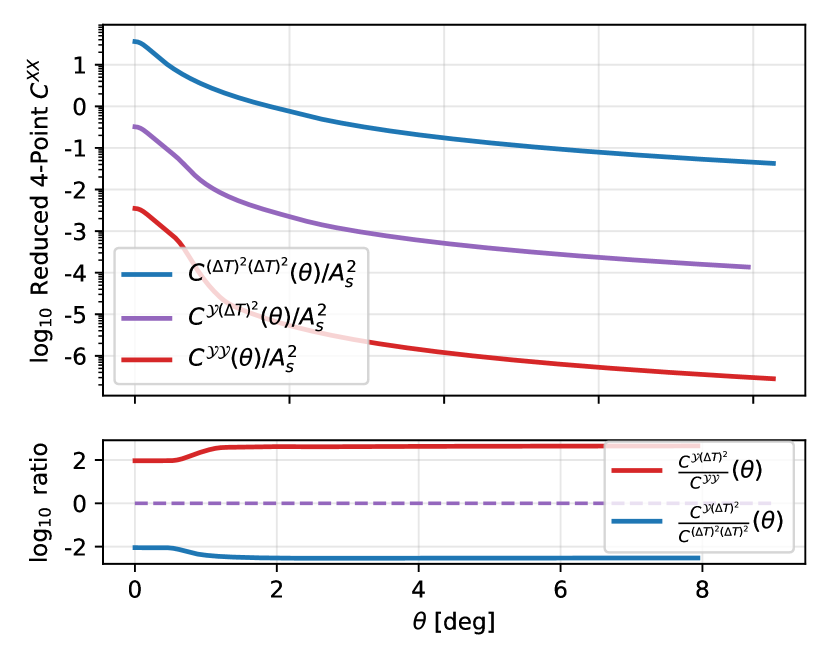
Figure 2: Upper panel: Reduced dimensionless angular correlation functions of $Y$, $C^{\mathcal{YY}}(\theta)/A_{s}^{2}$ (red), between $Y$ and $({\Delta T})^{2}$, $C^{\mathcal{Y}({\Delta T})^{2}}(\theta)/A_{s}^{2}$ (purple), and between the Sachs-Wolfe contributions to $({\Delta T})^{2}$, $C^{({\Delta T})^{2}({\Delta T})^{2}}(\theta)/A_{s}^{2}$ (blue), where $\theta$ is the angle between sky locations of the two quantities being correlated. Lower panel: the ratio of $C^{\mathcal{Y}({\Delta T})^{2}}$ to $C^{({\Delta T})^{2}({\Delta T})^{2}}$ (blue) and $C^{\mathcal{Y}({\Delta T})^{2}}$ to $C^{\mathcal{Y}\mathcal{Y}}$ (red).

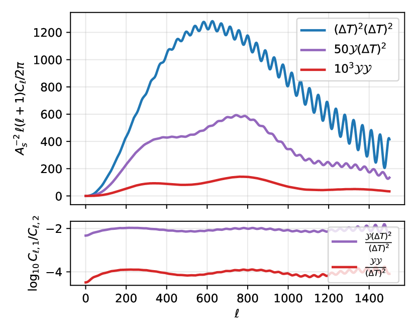
Figure 3: Upper panel: Legendre expansion coefficients (cf. (52)) of the correlation functions $C^{\mathcal{YY}}(\theta)/A_{s}^{2}$ (red) and $C^{\mathcal{Y}-({\Delta T})^{2}}(\theta)/A_{s}^{2}$ (purple), compared to those of $C^{({\Delta T})^{2}-({\Delta T})^{2}}(\theta)/A_{s}^{2}$ (blue), accounting solely for Sachs-Wolfe fluctuations. Lower panel: the ratio of the expansion coefficients to those of $({\Delta T})^{2}({\Delta T})^{2}$.

5 Detectability

The $\mathcal{Y}$ power spectrum is well below the detection capability of envisioned experiments, and is small compared to $\mathcal{Y}$ from low-redshift contributions. But the ${\mathcal{Y}}({\Delta T})^{2}$ cross power spectrum is more promising, because it has both a significantly larger amplitude and a distinctive shape, including slight imprints of acoustic oscillations, which can distinguish it from other contributions.

We estimate the detectability of $C_{\ell}^{\mathcal{Y}}({\Delta T})^{2}$ by assuming that both $\mathcal{Y}$ and $({\Delta T})^{2}$ are Gaussian random fields on the sky. While this is not precisely the case, it is a large simplification and should be sufficient for a reasonable signal-to-noise estimate. If the CMB blackbody temperature in a given sky pixel can be measured with an uncertainty of $\delta_{T}$, then the uncertainty in $({\Delta T})^{2}$ is $2{\Delta T}\delta_{T}+\delta_{T}^{2}$. Any map with a chance to detect the signal described here will have $\delta_{T}\ll{\Delta T}$ so the second term can be dropped. Since ${\Delta T}$ is itself normally distributed, it can be replaced by its rms value, so the uncertainty in $({\Delta T})^{2}$ is $\delta_{T^{2}}\simeq 2{\Delta T}_{\rm rms}\delta_{T}$. For a map of $\mathcal{Y}$, each pixel corresponds to a particular intensity distortion at each frequency, given by the usual thermal Sunyaev-Zeldovich formula. Taking 90 GHz as a typical frequency for ground-based experiments, an uncertainty in temperature $\delta_{T}$ gives $\delta_{Y}=1.6\delta_{T}/T_{0}$ as the uncertainty in $\mathcal{Y}$.

Given these pixel errors in two (approximately) Gaussian random fields, the uncertainty in measuring each $\ell$ mode of the angular cross-power spectrum $C_{\ell}^{\mathcal{Y}({\Delta T})^{2}}$ is analogous to determining $C_{\ell}^{TE}$ from maps of microwave background temperature and E-mode polarization. The variance, including both pixel noise and cosmic variance, is given by Kamionkowski et al. 1997, Eq. (3.26), as

$$\Xi_{\mathcal{Y}({\Delta T})^{2},\mathcal{Y}({\Delta T})^{2}}=\frac{1}{2\ell+1}\left[\left(C_{\ell}^{\mathcal{Y}({\Delta T})^{2}}\right)^{2}+\left(C_{\ell}^{({\Delta T})^{2}({\Delta T})^{2}}+w^{-1}_{({\Delta T})^{2}}\left(W_{\ell}^{b}\right)^{-2}\right)\left(C_{\ell}^{\mathcal{Y}\mathcal{Y}}+w^{-1}_{\mathcal{Y}}\left(W_{\ell}^{b}\right)^{-2}\right)\right]\,.$$ (53)

Here $w_{X}^{-1}\equiv 4\pi(\delta_{X}^{2})/N_{\rm pix}$ is the inverse statistical weight per unit solid angle on the sky for a map of some quantity with $N_{\rm pix}$ pixels and a pixel variance of $\delta^{2}$, and $W_{\ell}^{b}=\exp(-\ell^{2}\sigma_{b}^{2}/2)$ is the experiment beam profile in harmonic space, which is generally well approximated as a Gaussian with beam with $\sigma_{b}=\theta_{\rm fwhm}/\sqrt{8\ln 2}=1.2\times 10^{-4}(\theta_{\rm fwhm}/1^{\prime})$. The signal-to-noise with which a given $\ell$ mode can be measured is then just

$$\frac{\rm S}{\rm N}\left(C_{\ell}^{\mathcal{Y}({\Delta T})^{2}}\right)=\sqrt{(2\ell+1)f_{\rm sky}}\left[1+\left(\frac{C_{\ell}^{({\Delta T})^{2}({\Delta T})^{2}}}{C_{\ell}^{\mathcal{Y}({\Delta T})^{2}}}+\frac{w_{T^{2}}^{-1}\left(W_{\ell}^{b}\right)^{-2}}{C_{\ell}^{\mathcal{Y}({\Delta T})^{2}}}\right)\left(\frac{C_{\ell}^{\mathcal{Y}\mathcal{Y}}}{C_{\ell}^{\mathcal{Y}({\Delta T})^{2}}}+\frac{w_{\mathcal{Y}}^{-1}\left(W_{\ell}^{b}\right)^{-2}}{C_{\ell}^{\mathcal{Y}({\Delta T})^{2}}}\right)\right]^{-1/2}\,,$$ (54)

where a factor of $f_{\rm sky}$, giving the sky fraction covered by a map, has been included. To the extent the fields $\mathcal{Y}$ and $({\Delta T})^{2}$ are Gaussian, each mode is statistically independent, and the total signal-to-noise can be obtained by summing over all $\ell$ values probed by a given map.

As an example of the current experimental state of the art, we consider the ACT experiment (Coulton et al., 2023); maps of similar statistical weight and sky coverage have also been made by the SPT experiment (Bleem et al., 2022). Current ACT maps of the blackbody temperature component have uncertainties ranging from 5 $\mu$K to 14 $\mu$K per square arcminute; we take $\delta_{T}=10$ $\mu$K as a (conservative) mean temperature uncertainty. The final ACT data set provides maps with $f_{\rm sky}=0.33$, so for $(1^{\prime})^{2}$ pixels, $N_{\rm pix}=4.8\times 10^{7}$. The statistical weight factors are therefore $w^{-1}_{T}=2.6\times 10^{-5}$ $\mu{\rm K}^{2}$ and $w^{-1}_{({\Delta T})^{2}}=0.02$ $\mu{\rm K}^{4}$ (using $(\Delta T)_{\rm rms}=15\mu{\rm K}$). Dividing by factors of $T_{0}$ give the dimensionless values $w^{-1}_{T}=3.6\times 10^{-18}$ and $w^{-1}_{({\Delta T})^{2}}=3.8\times 10^{-28}$. Meanwhile $w^{-1}_{\cal Y}=(1.6)^{2}w^{-1}_{T}$. ACT considers measured $\ell$ values below about 500 to be potentially unreliable, so we only use multipole moments $\ell>500$.

For these parameters, the terms in eq. 54 containing $w_{({\Delta T})^{2}}^{-1}$ and $C_{\ell}^{\mathcal{Y}\mathcal{Y}}$ can be neglected, along with the $1$, so the expression simplifies to

$$\frac{\rm S}{\rm N}\left(C_{\ell}^{\mathcal{Y}({\Delta T})^{2}}\right)=\left(\frac{(2\ell+1)f_{\rm sky}}{C_{\ell}^{({\Delta T})^{2}({\Delta T})^{2}}w_{\mathcal{Y}}^{-1}}\right)^{1/2}C_{\ell}^{\mathcal{Y}({\Delta T})^{2}}W_{\ell}^{b}.$$ (55)

Summing from $\ell=500$ to $\ell=1500$ gives an expected total S/N of $12$ for ACT. So the diffusion spectral distortion should be detectable at current experiment sensitivities. SPT has released (Bleem et al., 2022) a y-distortion map with $1.25^{\prime}$ angular resolution, and approximately comparable quality to what we have assumed for ACT (although with a smaller $f_{\rm sky}$). The planned CMB-S4 experiment might improve on this by a factor of 10, principally by reducing $\delta_{T}$ to $\simeq 1\mu$K. This would allow robust detection of the acoustic oscillations in $C_{\ell}^{\mathcal{Y}({\Delta T})^{2}}$, and might therefore allow ${\cal Y}$ to be used as a cosmological probe analogous to polarization.

In forecasting the S/N, we have made several assumptions. Primarily, we have assumed that ${\cal Y}$ can be detected with uncertainty comparable to that in $\Delta T$. That requires robust foreground subtraction, since $\mathcal{Y}$ is large in the location of galaxy clusters, and the $\mathcal{Y}$ map will be dominated by distortions from foreground haloes. Since we are correlating with $({\Delta T})^{2}$, modeling this signal due to foreground $\mathcal{Y}$ contributions will likely be the primary challenge in extracting the recombination-era signal. We have also worked in the approximation that ${\cal Y}$ and $(\Delta T)^{2}$ are Gaussian, which they are not, and a more careful statistical treatment is merited. Finally, we have included only the Sachs-Wolfe contribution to the transfer function, and used an analytic approximation.

6 Discussion and Conclusions

In this paper we provide a real-space description of the $y$-type spectral distortion of the CMB that arises from the scattering of the photons into our line of sight (Zel’dovich et al., 1972). Each photon’s scattering history is different, sampling both radially along and transverse to the line of sight through the recombination era. Because the photons’ final scatterings make nearly no change to the photon energy, the resulting distribution of photon energies that we observe is a mixture of blackbody distributions of different temperatures, representing the inhomogeneity of the temperature in the region from which the photons originated.

This “diffusion spectral distortion” is, like the CMB intensity (temperature) and polarization, a probe of the acoustic modes responsible for the inhomogeneities in the universe during the epoch of recombination. Like the E-mode polarization and the temperature, in standard $\Lambda$ Cold Dark Matter cosmology, the diffusion spectral distortion signal is partly, but not perfectly, correlated with these other signals. For example, while the E-mode fluctuations probe the local quadrupole of the temperature distribution, the diffusion spectral distortion is also sensitive to its dipole.

Diffusion spectral distortion offers another independent probe of the physics at the end of recombination. Inherently, this implies the opportunity to reduce cosmic variance on existing measurements of quantities probed by the temperature and polarization. Additionally, because it is sensitive to the variation in the photon temperature along the line-of-sight, diffusion spectral distortion could potentially be the basis of a new Alcock-Paczynski test (Alcock & Paczynski, 1979) at the epoch of recombination. It could also allow us to test statistical isotropy at the epoch of recombination, complementing the large scale tests traditionally done with temperature that have yielded anomalous results (Schwarz et al., 2016; Planck Collaboration et al., 2020b; Abdalla et al., 2022). Diffusion spectral distortion is therefore both a consistency check for the standard cosmological model and sensitive to new physics in a way that is complementary to other signals.

Polarization is also generated during recombination, and usually described as a measure of the local quadrupole at the last scattering. The polarization spectrum and its distortion away from blackbody are therefore due to a different weighted sum over blackbodies, with the potential for yet another signal complementary to the one we have described. This is another step towards a possible tomographic probe (Yadav & Wandelt, 2005) of the universe through recombination.

Current and upcoming experiments will not be sufficiently sensitive to the $y$-type distortion to measure the diffusion spectral distortion signal directly. In part, the challenge is insufficient signal-to-noise. However, a greater challenge is likely to be separation of the component of the $y$-distortion due to recombination-era diffusion from other causes of spectral distortion in the presence of foregrounds with spectra that are imperfectly known and that are also anisotropic (Abitbol et al., 2017b; Hart et al., 2020). These foregrounds include our Milky Way, and both galaxies and galaxy clusters at all redshifts. The $\mathcal{Y}$ auto-correlation function, like the $y$-type distortion, will not be detectable by current or upcoming experiments. The amplitude of the correlation signal is far smaller than for other sources of $y$ auto-correlation at low redshifts, and so will be difficult to separate from foregrounds.

More promising than the $\mathcal{Y}$ signal itself or its auto-correlation function is the cross-correlation $C_{\ell}^{\mathcal{Y}({\Delta T})^{2}}$ between the $y$-distortion and the square of the temperature fluctuations. (The $\mathcal{Y}$-$T$ correlation will be zero if the primordial photon perturbations are a Gaussian field.) This is calculated in §​ 4. Like the temperature fluctuations, the diffusion spectral distortion, and hence their cross-correlation function, contains acoustic features. The combination of the specific spectral shape and the correlation with the primordial temperature fluctuations should facilitate the separation of this correlation function from foreground signals. Galactic foreground confusion is uncorrelated with primordial temperature anisotropies (though of course it would be correlated with any residual unsubtracted Galactic temperature foreground). Extragalactic foregrounds are concentrated at galaxy clusters (which are detected at high significance) and at galaxies. Fortunately, the clusters can be masked and are relatively sparse on the sky. Galaxies are far more numerous and non-sparsely distributed; however, the amplitude of the galaxy confusion limit $y$-distortion is also small and would have a different correlation function with the temperature fluctuations.

The three-point correlation function between $\mathcal{Y}({\bf\hat{n}}_{1})$, ${\Delta T}({\bf\hat{n}}_{2})$, and ${\Delta T}({\bf\hat{n}}_{3})$ at three different points may also be detectably large. Considering different configurations of this three-point function will give further handles on separating the diffusion distortion from various foreground contributions (Coulton et al., 2018). Calculation of this signal is more complicated than the two-point function and will be considered elsewhere.

In §​ 5 we determined that multi-frequency maps over a third of the sky with the $10\mu$K–arcmin sensitivity attained by the final ACT dataset (Coulton et al., 2023) have sufficient sensitivity to detect this signal, and SPT has achieved similar reach (Bleem et al., 2022). Sky maps with sensitivities approaching 1 $\mu$K–arcmin are anticipated in the next decade (Abitbol et al., 2017a). Sufficient frequency coverage is required to separate the $y$-distortion from the primary blackbody and other spectrum components.

Our signal and sensitivity calculations involved several simplifying assumptions. More rigorous calculations of the $y$-distortion and its correlation with the temperature and polarization anisotropies during diffusion damping are warranted. Ultimately, a complete calculation of the statistics of spectral distortions arising from physical processes around last scattering may reveal additional probes of the cosmological model, providing substantial consistency checks or additional handles on non-standard physics.

Data Availability

This study was carried out using the reproducibility software (Luger et al., 2021), which uses continuous integration to programmatically download the data, perform the analyses, create the figures, and compile the manuscript. Each figure caption contains two links: one to the dataset used in the corresponding figure, and the other to the script used to make the figure. The datasets are stored at https://zenodo.org/record/8400583. The git repository associated with this study is publicly available at nstarman/Temperature-Diffusion-Spectral-Distortion-Paper.

Appendix A Coordinate Systems

We use the standard definition of the scale factor: $a(z=\infty)=0$, $a(z=0)=1$.

For analytic simplicity, we consider a two component universe containing only matter and radiation, whose energy densities were equal when the value of the scale factor was $a_{\rm eq}$, or equivalently at redshift $z_{\rm eq}$. This is an excellent approximation during the epoch of recombination and last scattering, when all the complex physics of this problem takes place. Of course it is a poor approximation thereafter, but that is easily accounted for by placing a reference observer at a redshift much less than that of last scattering, but much greater than that of cosmological constant dominance. We are therefore able to take $z_{\rm eq}$ to be its inferred value from observations; in particular $z_{\rm eq}=(\Omega_{m}/\Omega_{r}-1)=3404$ from Planck Collaboration et al. (2020a).

The comoving distance along a photon’s path from a point a with scale factor $a_{i}$ to a point with scale factor $a_{f}>a_{i}$ is

$$r(a_{i},a_{f}) =\frac{L_{\rm eq}}{\sqrt{8a_{\rm eq}}}\int_{a_{i}}^{a_{f}}\frac{\mathrm{d}{a^{\prime}}}{\sqrt{a_{\rm eq}+a^{\prime}}}=L_{\rm eq}\left.\sqrt{\frac{1+a/a_{\rm eq}}{2}}\right|_{a_{i}}^{a_{f}}\,,$$ (56)

where

$$L_{\rm eq}\equiv\frac{c}{H_{0}}\sqrt{\frac{8\,a_{\rm eq}}{\Omega_{m,0}}}$$ (57)

It proves convenient, for calculating $\mathcal{P}(s_{||},s_{\perp},\phi)$ eq. 10, to use dimensionless comoving distances that are anchored, time-oriented, and of a convenient magnitude during recombination. We define

$$\rho(z)\equiv\sqrt{\frac{1}{2}\left(1+\frac{1+z_{\rm eq}}{1+z}\right)}\,.$$ (58)

Useful special cases are: $\rho_{\rm eq}=1$, and $\rho(z=\infty)\equiv 1/\sqrt{2}$. Because we are using a matter-plus-radiation approximation for the evolution of the scale factor, we cannot use our definition of $\rho$ for late times, for example today ($z=0$). We take $\rho_{o}$ to be the largest allowed value of $\rho$, taken at $z=z_{o}=100$. Now,

$$r(z_{i},z_{f})=L_{\rm eq}\;(\rho(z_{f})-\rho(z_{i}))$$ (59)

Appendix B Visibility Function

The epoch of recombination was not instantaneous, and the universe did not become transparent instantaneously, so CMB photons did not propagate unimpeded from some fixed epoch. The visibility function is the probability per-unit-distance that a photon observed at position $x_{2}$ last interacted at position $x_{1}$. Abramo et al. (2010, eq. 1-3) gives a very good explanation of the visibility function, phrased in terms of the conformal time $\eta$, with $ad\eta\equiv dt$. We list the important terms, noting small changes to notation and that we express quantities as functions of redshift not conformal time:

• $\bar{\mu}(z_{1},z_{2})$, the optical depth for Thompson scattering;

• $\overline{P_{\gamma}}(z_{1},z_{2})=e^{-\bar{\mu}(z_{1},z_{2})}$, the total visibility;

• $\overline{g_{\gamma}}(z_{1},z_{2})=\frac{\mathrm{d}{z_{1}}}{\mathrm{d}{\eta_{1}}}\frac{\mathrm{d}{}}{\mathrm{d}{z_{1}}}\overline{P_{\gamma}}(z_{1},z_{2})$, the visibility function, which is the likelihood of a photon Thompson scattering between redshifts $z_{1}$ and $z_{2}$.

The overbar in $\bar{\mu}$, $\overline{P_{\gamma}}$, and $\overline{g_{\gamma}}$ indicates that they are functions only of $z$ and not position, as they refer to the unperturbed ‘‘background cosmology".

For numerical and analytic purposes, we want to ‘‘split" our background quantities, i.e. we rewrite $\overline{P_{\gamma}}(z_{1},z_{2})$ (where $z_{2}<z_{1})$ in terms of CLASS’s $\overline{P_{\gamma}}^{CL}(z)$ which is anchored at the observer $z_{O}$:

$$\overline{P_{\gamma}}^{CL}(z) =\overline{P_{\gamma}}(z,z_{O})=e^{-\mu(z,z_{O})}$$

 For this we write

$$\overline{P_{\gamma}}(z_{1},z_{2}) =\frac{\overline{P_{\gamma}}(z_{1},z_{O})}{\overline{P_{\gamma}}(z_{2},z_{O})}=\frac{\overline{P_{\gamma}}^{CL}(z_{1})}{\overline{P_{\gamma}}^{CL}(z_{2})} \,.$$ (60)

Similarly, for $\overline{g_{\gamma}}$:

$$\overline{g_{\gamma}}^{CL}(z) =\overline{g_{\gamma}}(z,z_{O})\,,$$ (61)

 and so

$$\overline{g_{\gamma}}(z_{1},z_{2}) =\frac{\mathrm{d}{z_{1}}}{\mathrm{d}{\eta_{1}}}\frac{\mathrm{d}}{\mathrm{d}{z_{1}}}\left({e^{-\mu(z_{1},z_{2})}}\right)=\frac{\mathrm{d}{z_{1}}}{\mathrm{d}{\eta_{1}}}\frac{\mathrm{d}}{\mathrm{d}{z_{1}}}\left({\frac{e^{-\mu(z_{1},z_{O})}}{e^{-\mu(z_{2},z_{O})}}}\right)=\frac{1}{e^{-\mu(z_{2},z_{O})}}\frac{\mathrm{d}{z_{1}}}{\mathrm{d}{\eta_{1}}}\frac{\mathrm{d}}{\mathrm{d}{z_{1}}}\left({e^{-\mu(z_{1},z_{O})}}\right)=\frac{\overline{g_{\gamma}}^{CL}(z_{1})}{\overline{P_{\gamma}}^{CL}(z_{2})}\,.$$ (62)

Appendix C Calculating and Sampling $\mathcal{P}(s_{||},s_{\perp},\phi)$

For calculating and sampling $\mathcal{P}$, it is convenient to perform a change of coordinates. In eq. 7 we define $s_{||},s_{\perp}$, and in eq. 58 we define $\rho$. We define

$$\overline{g_{\gamma}}(\rho_{2},\rho_{1})\equiv\overline{g_{\gamma}}(z_{2},z_{1})\,,$$ (63)

normalized such that $L_{\rm eq}\int\!\mathrm{d}{\rho_{2}}\;\overline{g_{\gamma}}(\rho_{2},\rho_{1})=1$.

Rewriting eq. 10 in terms of $\rho_{i}$ and the CLASS-defined functions,

$$\mathcal{P}(s_{||},s_{\perp},\phi) =\frac{3L_{\rm eq}^{2}}{16\pi\overline{P_{\gamma}}^{CL}(\rho_{O})}\int\!\!\!\mathrm{d}{\rho_{1}}\;\overline{g_{\gamma}}^{CL}(\rho_{1})\frac{\overline{g_{\gamma}}^{CL}\left(\rho_{1}\!-\!\sqrt{(\rho_{1}+s_{||}-\rho_{O})^{2}+s_{\perp}^{2}}\right)}{\overline{P_{\gamma}}^{CL}(\rho_{1})}\frac{(2(\rho_{1}+s_{||}-\rho_{O})^{2}+s_{\perp}^{2})s_{\perp}}{\left((\rho_{1}+s_{||}-\rho_{O})^{2}+s_{\perp}^{2}\right)^{2}}\,,$$ (64)

which we evaluate as follows. For a given $s_{||},s_{\perp}$ we perform a cubic spline in $\rho_{1}$ of

$$f(\rho_{1};s_{||}-\rho_{O},s_{\perp})\equiv\frac{\overline{g_{\gamma}}^{CL}(\rho_{1})}{\overline{P_{\gamma}}^{CL}(\rho_{1})}{\overline{g_{\gamma}}^{CL}\left(\rho_{1}\!-\!\sqrt{(\rho_{1}+s_{||}-\rho_{O})^{2}+s_{\perp}^{2}}\right)}\,.$$ (65)

Between knots of the spline ($\rho_{1}\in[\rho_{1}^{(i)},\rho_{1}^{(i)}]$), we must do the integral

$$\sum_{j=0}^{3}f_{j}^{(i)}(s_{||}-\rho_{O},s_{\perp})\int_{\rho_{1}^{(i)}}^{\rho_{1}^{(i+1)}}\!\!\!\!\!\mathrm{d}{\rho_{1}}\;\rho_{1}^{j}~{}\frac{(2(\rho_{1}+s_{||}-\rho_{O})^{2}+s_{\perp}^{2})s_{\perp}}{\left((\rho_{1}+s_{||}-\rho_{O})^{2}+s_{\perp}^{2}\right)^{2}}\,.$$ (66)

The integrals with different $\rho_{1}^{j}$ can all be done analytically:

$$\bullet\int\!\mathrm{d}{\rho_{1}}\,\rho_{1}^{0}~{}\frac{(2(\rho_{1}+s_{||}-\rho_{O})^{2}+s_{\perp}^{2})s_{\perp}}{\left((\rho_{1}+s_{||}-\rho_{O})^{2}+s_{\perp}^{2}\right)^{2}} =-\frac{s_{\perp}(\rho_{1}+s_{||}-\rho_{O})}{2\left((\rho_{1}+s_{||}-\rho_{O})^{2}+s_{\perp}^{2}\right)}+\frac{3}{2}\arctan{\left(\frac{\rho_{1}+s_{||}-\rho_{O}}{s_{\perp}}\right)}\,,$$ (67)

$$\bullet\int\!\mathrm{d}{\rho_{1}}\,\rho_{1}~{}\frac{(2(\rho_{1}+s_{||}-\rho_{O})^{2}+s_{\perp}^{2})s_{\perp}}{\left((\rho_{1}+s_{||}-\rho_{O})^{2}+s_{\perp}^{2}\right)^{2}} =\frac{s_{\perp}(s_{||}-\rho_{O})(\rho_{1}+s_{||}-\rho_{O})+s_{\perp}^{3}}{2((\rho_{1}+(s_{||}-\rho_{O}))^{2}+s_{\perp}^{2})}-\frac{3}{2}(s_{||}-\rho_{O})\arctan\left(\frac{\rho_{1}+s_{||}-\rho_{O}}{s_{\perp}}\right)$$ (68)

$$\phantom{=}+s_{\perp}\ln\left[(\rho_{1}+s_{||}-\rho_{O})^{2}+s_{\perp}^{2}\right]\,,$$

$$\bullet\int\!\mathrm{d}{\rho_{1}}\,\rho_{1}^{2}~{}\frac{(2(\rho_{1}+s_{||}-\rho_{O})^{2}+s_{\perp}^{2})s_{\perp}}{\left((\rho_{1}+s_{||}-\rho_{O})^{2}+s_{\perp}^{2}\right)^{2}} =\frac{5}{2}\rho_{1}s_{\perp}-\frac{1}{2}(s_{||}-\rho_{O})s_{\perp}-\frac{\rho_{1}^{2}s_{\perp}(\rho_{1}+s_{||}-\rho_{O})}{2((\rho_{1}+(s_{||}-\rho_{O}))^{2}+s_{\perp}^{2})}$$ (69)

$$\phantom{=}+\frac{1}{2}\left(3(s_{||}-\rho_{O})^{2}-5s_{\perp}^{2}\right)\arctan\left(\frac{\rho_{1}+s_{||}-\rho_{O}}{s_{\perp}}\right)$$

$$\phantom{=}-2(s_{||}-\rho_{O})s_{\perp}\ln\left[(\rho_{1}+s_{||}-\rho_{O})^{2}+s_{\perp}^{2}\right]\,,$$

$$\bullet\int\!\mathrm{d}{\rho_{1}}\,\rho_{1}^{3}~{}\frac{(2(\rho_{1}+s_{||}-\rho_{O})^{2}+s_{\perp}^{2})s_{\perp}}{\left((\rho_{1}+s_{||}-\rho_{O})^{2}+s_{\perp}^{2}\right)^{2}} =\frac{1}{2}s_{\perp}\left(3\rho_{1}^{2}-9\rho_{1}(s_{||}-\rho_{O})+(s_{||}-\rho_{O})^{2}-s_{\perp}^{2}\right)$$ (70)

$$\phantom{=}-\frac{\rho_{1}^{3}s_{\perp}(\rho_{1}+s_{||}-\rho_{O})}{2((\rho_{1}+s_{||}-\rho_{O})^{2}+s_{\perp}^{2})}$$

$$\phantom{=}-\frac{3}{2}(s_{||}-\rho_{O})\left[(s_{||}-\rho_{O})^{2}-5s_{\perp}^{2}\right]\arctan\left(\frac{\rho_{1}+s_{||}-\rho_{O}}{s_{\perp}}\right)$$

$$\phantom{=}+3s_{\perp}\left((s_{||}-\rho_{O})^{2}-\frac{1}{2}s_{\perp}^{2}\right)\ln\left[(\rho_{1}+(s_{||}-\rho_{O}))^{2}+s_{\perp}^{2}\right]\,.$$

We take particular care to ensure that $\rho_{1}=\rho_{O}-s_{||}$ is not one of the knots of the spline, because the integral is numerically unstable (though not analytically problematic) if an integral bound (knot point) is too close to this value.

To do the full integral we need to know the range of $s_{||}$ and $s_{\perp}$ over which we should evaluate $\mathcal{P}$. We therefore identify a range $\rho_{\rm min}<\rho<\rho_{\rm max}$ over which $\overline{g_{\gamma}}$ is above its value at $z_{0}$. Requiring that

$$\rho_{\rm min}<\rho_{1}<\rho_{\rm max}$$ (71)

sets the range over which we integrate in eq. 64 while demanding that

$$\rho_{\rm min}<\rho_{1}-\sqrt{(\rho_{1}+s_{||}-\rho_{O})^{2}+s_{\perp}^{2}}<\rho_{\rm max}$$ (72)

sets the range of $s_{||}$ and $s_{\perp}$ as a function of $\rho_{1}$. Rewriting the first inequality of eq. 72,

$$\sqrt{(\rho_{1}+s_{||}-\rho_{O})^{2}+s_{\perp}^{2}}<\rho_{1}-\rho_{\rm min}$$ (73)

and so

$$(\rho_{1}+s_{||}-\rho_{O})^{2}+s_{\perp}^{2}<(\rho_{1}-\rho_{\rm min})^{2}\,.$$ (74)

Since the right hand side is largest when $\rho_{1}=\rho_{\rm max}$, we require

$$(\rho_{1}+s_{||}-\rho_{O})^{2}+s_{\perp}^{2}<(\rho_{\rm max}-\rho_{\rm min})^{2}\,.$$ (75)

We see that we must range over

$$0\leq s_{\perp}\leq\rho_{\rm max}-\rho_{\rm min}$$ (76)

Rewriting eq. 74, $s_{||}$ must be between the two roots $\sigma_{\pm}$ of the polynomial

$$P(s_{||})\equiv s_{||}^{2}+2s_{||}(\rho_{1}-\rho_{O})+(\rho_{1}-\rho_{O})^{2}+s_{\perp}^{2}-(\rho_{1}-\rho_{\rm min})^{2}$$

Thus

$$\sigma_{\pm}=\rho_{O}-\rho_{1}\pm\sqrt{(\rho_{1}-\rho_{\rm min})^{2}+s_{\perp}^{2}}$$ (77)

This translates to

$$\rho_{O}-\rho_{\rm min}\leq s_{||}\leq\rho_{O}-2\rho_{\rm max}+\rho_{\rm min}\leq-\rho_{O}+\rho_{\rm min}$$ (78)

For the obvious choice of $\rho_{\rm max}=\rho_{O}$, we get

$$-\rho_{O}+\rho_{\rm min}\leq s_{||}\leq\rho_{O}-\rho_{\rm min}\,,$$ (79)

which is nicely symmetric about $0$.

Constant values of $\rho_{2}\leq\rho_{1}$ are circles in $(s_{||},s_{\perp})$, with center $\rho_{O}-\rho_{1}$ and radius $\rho_{1}-\rho_{2}$. Of course we can never have $\rho_{2}>\rho_{1}$. We note that $\overline{g_{\gamma}}^{CL}(\rho)$ peaks at $\rho=\rho_{R}$ (recombination), so if $\rho_{1}<\rho_{R}$, then so is $\rho_{2}$, and $\overline{g_{\gamma}}^{CL}(\rho_{2})$ never reaches its peak value. However, if $\rho_{1}>\rho_{R}$, then $\overline{g_{\gamma}}^{CL}(\rho_{2}=\rho_{R})$ is a circle of radius $\rho_{1}-\rho_{R}$, and center $\rho_{O}-\rho_{1}$. These intersect $s_{\perp}=0$ at $s_{||}=\rho_{O}-\rho_{R}$ and $s_{||}=\rho_{O}+\rho_{R}-2\rho_{1}$.

The Monte Carlo integration of eq. 26 requires drawing samples from $\mathcal{P}(s_{||},s_{\perp},\phi)$, (defined in eq. 10 and eq. 64). The $\phi$ component is separable and can be trivially sampled from $\phi\sim U(0,2\pi)$. The $s_{||}$ and $s_{\perp}$ distributions are not separable. To sample from $\mathcal{P}(s_{||},s_{\perp})\equiv 2\pi\mathcal{P}(s_{||},s_{\perp},\phi)$ we first sample $s_{||}$ from the marginal distribution distribution $\mathcal{P}(s_{||})=\int_{s_{\perp}}\!\mathrm{d}{s_{\perp}}\,\mathcal{P}(s_{||},s_{\perp})$. Then we sample $s_{\perp}$ from the conditional distribution $\mathcal{P}(s_{\perp}|s_{||})$. Fig. 4 shows the set of sampled points used in §​ 3 and Appendix Appendix D.

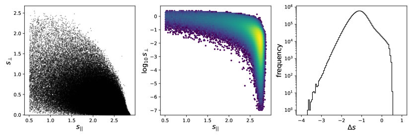
Figure 4: 10 million points sampled from $\mathcal{P}$. Left: $\mathcal{P}$ the samples in $s_{||},s_{\perp}$. The probability density function is negligible for $s_{||}<0.5$, so we do not sample past this point. Middle: same sample as left, plotting as a density histogram and in logarithmic coordinates for $s_{\perp}$. The density coloring emphasizes that $s_{||}<0.5$ is not important to the results. The logarithmic coordinates shows that while $s_{\perp}$ extends to 0 analytically, it is sampled linearly and thus decreases a factor of ten in sampled density for every decade in $s_{\perp}\rightarrow 0$. Our results are limited not by sampling $s_{\perp}$ close to 0, but by samples of $\Delta s$ near 0. Right: showing the distribution of $\Delta s$. The maximum separation is set by $(s_{||},s_{\perp})=\lvert(\rm{min},\rm{max})-(\rm{max},\rm{min})\rvert\approx 3.2$. The minimum separation is approximate $10^{-4}$, though may be decreased at the cost of sampling more points from $\mathcal{P}$.

Appendix D Calculating the Correlation

Calculating the correlation of $\mathcal{Y}({\bf\hat{n}}_{1})$ with $\Delta T^{l}({\bf\hat{n}}_{2})$ is straightforward, if delicate, involving taking and simplifying many expectation values. We do not leave this as an exercise to the reader.

$$\frac{1}{T_{0}^{2}}\mathcal{Y}({\bf\hat{n}}_{1})({\Delta T}^{l}({\bf\hat{n}}_{2}))^{2} =\frac{1}{2T_{0}^{4}}\Bigg{[}\int\!\!\!\mathrm{d}{\mathbf{s}_{1}}\;\mathcal{P}(\mathbf{s}_{1})\left({\Delta T}^{e}(\mathbf{x}({\bf\hat{n}}_{1},\mathbf{s}_{1}))\right)^{2}-\int\!\!\mathrm{d}{\mathbf{s}_{1}}\mathcal{P}(\mathbf{s}_{1})\mathrm{d}{\mathbf{s}^{\prime}_{1}}\mathcal{P}(\mathbf{s}^{\prime}_{1}){\Delta T}^{e}(\mathbf{x}({\bf\hat{n}}_{1},\mathbf{s}_{1})){\Delta T}^{e}(\mathbf{x}({\bf\hat{n}}_{1},\mathbf{s}^{\prime}_{1}))\Bigg{]}$$ (80)

$$\qquad\times\int\!\!\mathrm{d}{\mathbf{s}_{2}}\mathcal{P}(\mathbf{s}_{2})\mathrm{d}{\mathbf{s}^{\prime}_{2}}\mathcal{P}(\mathbf{s}^{\prime}_{2}){\Delta T}^{l}(\mathbf{x}({\bf\hat{n}}_{2},\mathbf{s}_{2})){\Delta T}^{l}(\mathbf{x}({\bf\hat{n}}_{2},\mathbf{s}^{\prime}_{2}))$$

$$=\frac{1}{2T_{0}^{4}}\Bigg{[}\phantom{+}\int\!\!\mathrm{d}{\mathbf{s}_{1}}\mathcal{P}(\mathbf{s}_{1})\mathrm{d}{\mathbf{s}_{2}}\mathcal{P}(\mathbf{s}_{2})\mathrm{d}{\mathbf{s}^{\prime}_{2}}\mathcal{P}(\mathbf{s}^{\prime}_{2})\left({\Delta T}^{e}(\mathbf{x}({\bf\hat{n}}_{1},\mathbf{s}_{1}))\right)^{2}{\Delta T}^{l}(\mathbf{x}({\bf\hat{n}}_{2},\mathbf{s}_{2})){\Delta T}^{l}(\mathbf{x}({\bf\hat{n}}_{2},\mathbf{s}^{\prime}_{2}))$$ (81)

$$\qquad\quad-\int\!\!\mathrm{d}{\mathbf{s}_{1}}\mathcal{P}(\mathbf{s}_{1})\mathrm{d}{\mathbf{s}^{\prime}_{1}}\mathcal{P}(\mathbf{s}^{\prime}_{1})\mathrm{d}{\mathbf{s}_{2}}\mathcal{P}(\mathbf{s}_{2})\mathrm{d}{\mathbf{s}^{\prime}_{2}}\mathcal{P}(\mathbf{s}^{\prime}_{2}){\Delta T}^{e}(\mathbf{x}({\bf\hat{n}}_{1},\mathbf{s}_{1})){\Delta T}^{e}(\mathbf{x}({\bf\hat{n}}_{1},\mathbf{s}^{\prime}_{1})){\Delta T}^{l}(\mathbf{x}({\bf\hat{n}}_{2},\mathbf{s}_{2})){\Delta T}^{l}(\mathbf{x}({\bf\hat{n}}_{2},\mathbf{s}^{\prime}_{2}))\Bigg{]}\,.$$

Taking the expectation value,

$$2T_{0}^{4}\langle\frac{1}{T_{0}^{2}}\mathcal{Y}({\bf\hat{n}}_{1})({\Delta T}^{l}({\bf\hat{n}}_{2}))^{2}\rangle =\phantom{+}\int\!\!\mathrm{d}{\mathbf{s}_{1}}\mathcal{P}(\mathbf{s}_{1})\mathrm{d}{\mathbf{s}_{2}}\mathcal{P}(\mathbf{s}_{2})\mathrm{d}{\mathbf{s}^{\prime}_{2}}\mathcal{P}(\mathbf{s}^{\prime}_{2})\Big{\langle}\left({\Delta T}^{e}(\mathbf{x}({\bf\hat{n}}_{1},\mathbf{s}_{1})\right)^{2}){\Delta T}^{l}(\mathbf{x}({\bf\hat{n}}_{2},\mathbf{s}_{2})){\Delta T}^{l}(\mathbf{x}({\bf\hat{n}}_{2},\mathbf{s}^{\prime}_{2}))\Big{\rangle}$$ (82)

$$\quad-\int\!\!\mathrm{d}{\mathbf{s}_{1}}\mathcal{P}(\mathbf{s}_{1})\mathrm{d}{\mathbf{s}^{\prime}_{1}}\mathcal{P}(\mathbf{s}^{\prime}_{1})\mathrm{d}{\mathbf{s}_{2}}\mathcal{P}(\mathbf{s}_{2})\mathrm{d}{\mathbf{s}^{\prime}_{2}}\mathcal{P}(\mathbf{s}^{\prime}_{2})\Big{\langle}{\Delta T}^{e}(\mathbf{x}({\bf\hat{n}}_{1},\mathbf{s}_{1})){\Delta T}^{e}(\mathbf{x}({\bf\hat{n}}_{1},\mathbf{s}^{\prime}_{1})){\Delta T}^{l}(\mathbf{x}({\bf\hat{n}}_{2},\mathbf{s}_{2})\Delta)T^{l}(\mathbf{x}({\bf\hat{n}}_{2},\mathbf{s}^{\prime}_{2})\Big{\rangle}$$

$$=\phantom{+}\int\!\!\mathrm{d}{\mathbf{s}_{1}}\mathcal{P}(\mathbf{s}_{1})\mathrm{d}{\mathbf{s}_{2}}\mathcal{P}(\mathbf{s}_{2})\mathrm{d}{\mathbf{s}^{\prime}_{2}}\mathcal{P}(\mathbf{s}^{\prime}_{2})\Big{\langle}\left({\Delta T}^{e}(\mathbf{x}({\bf\hat{n}}_{1},\mathbf{s}_{1})\right)^{2})\Big{\rangle}\Big{\langle}{\Delta T}^{l}(\mathbf{x}({\bf\hat{n}}_{2},\mathbf{s}_{2})){\Delta T}^{l}(\mathbf{x}({\bf\hat{n}}_{2},\mathbf{s}^{\prime}_{2}))\Big{\rangle}$$

$$\quad+2\int\!\!\mathrm{d}{\mathbf{s}_{1}}\mathcal{P}(\mathbf{s}_{1})\mathrm{d}{\mathbf{s}_{2}}\mathcal{P}(\mathbf{s}_{2})\mathrm{d}{\mathbf{s}^{\prime}_{2}}\mathcal{P}(\mathbf{s}^{\prime}_{2})\Big{\langle}{\Delta T}^{e}(\mathbf{x}({\bf\hat{n}}_{1},\mathbf{s}_{1})){\Delta T}^{l}(\mathbf{x}({\bf\hat{n}}_{2},\mathbf{s}_{2}))\Big{\rangle}\Big{\langle}{\Delta T}^{e}(\mathbf{x}({\bf\hat{n}}_{1},\mathbf{s}_{1})){\Delta T}^{l}(\mathbf{x}({\bf\hat{n}}_{2},\mathbf{s}^{\prime}_{2}))\Big{\rangle}$$

$$\quad-\int\!\!\mathrm{d}{\mathbf{s}_{1}}\mathcal{P}(\mathbf{s}_{1})\mathrm{d}{\mathbf{s}^{\prime}_{1}}\mathcal{P}(\mathbf{s}^{\prime}_{1})\mathrm{d}{\mathbf{s}_{2}}\mathcal{P}(\mathbf{s}_{2})\mathrm{d}{\mathbf{s}^{\prime}_{2}}\mathcal{P}(\mathbf{s}^{\prime}_{2})\Bigg{[}\phantom{+}\Big{\langle}{\Delta T}^{e}(\mathbf{x}({\bf\hat{n}}_{1},\mathbf{s}_{1})){\Delta T}^{e}(\mathbf{x}({\bf\hat{n}}_{1},\mathbf{s}^{\prime}_{1}))\Big{\rangle}\Big{\langle}{\Delta T}^{l}(\mathbf{x}({\bf\hat{n}}_{2},\mathbf{s}_{2})){\Delta T}^{l}(\mathbf{x}({\bf\hat{n}}_{2},\mathbf{s}^{\prime}_{2}))\Big{\rangle}$$

$$\qquad\qquad\qquad\qquad\qquad\qquad\qquad\qquad\qquad\quad+\Big{\langle}{\Delta T}^{e}(\mathbf{x}({\bf\hat{n}}_{1},\mathbf{s}_{1})){\Delta T}^{l}(\mathbf{x}({\bf\hat{n}}_{2},\mathbf{s}_{2}))\Big{\rangle}\Big{\langle}{\Delta T}^{e}(\mathbf{x}({\bf\hat{n}}_{1},\mathbf{s}^{\prime}_{1})){\Delta T}^{l}(\mathbf{x}({\bf\hat{n}}_{2},\mathbf{s}^{\prime}_{2}))\Big{\rangle}$$

$$\qquad\qquad\qquad\qquad\qquad\qquad\qquad\qquad\qquad\quad+\Big{\langle}{\Delta T}^{e}(\mathbf{x}({\bf\hat{n}}_{1},\mathbf{s}_{1})){\Delta T}^{l}(\mathbf{x}({\bf\hat{n}}_{2},\mathbf{s}^{\prime}_{2}))\Big{\rangle}\Big{\langle}{\Delta T}^{e}(\mathbf{x}({\bf\hat{n}}_{1},\mathbf{s}^{\prime}_{1})){\Delta T}^{l}(\mathbf{x}({\bf\hat{n}}_{2},\mathbf{s}_{2}))\Big{\rangle}\Bigg{]}$$

$$=\phantom{+}\int\!\!\mathrm{d}{\mathbf{s}_{2}}\mathcal{P}(\mathbf{s}_{2})\mathrm{d}{\mathbf{s}^{\prime}_{2}}\mathcal{P}(\mathbf{s}^{\prime}_{2})\xi^{ee}(0)\xi^{ll}\left(\lvert\mathbf{x}({\bf\hat{n}}_{2},\mathbf{s}_{2})-\mathbf{x}({\bf\hat{n}}_{2},\mathbf{s}^{\prime}_{2})\rvert\right)$$

$$\quad+2\int\!\!\mathrm{d}{\mathbf{s}_{1}}\mathcal{P}(\mathbf{s}_{1})\mathrm{d}{\mathbf{s}_{2}}\mathcal{P}(\mathbf{s}_{2})\mathrm{d}{\mathbf{s}^{\prime}_{2}}\mathcal{P}(\mathbf{s}^{\prime}_{2})\xi^{el}\left(\lvert\mathbf{x}({\bf\hat{n}}_{1},\mathbf{s}_{1})-\mathbf{x}({\bf\hat{n}}_{2},\mathbf{s}_{2})\rvert\right)\xi^{el}\left(\lvert\mathbf{x}({\bf\hat{n}}_{1},\mathbf{s}_{1})-\mathbf{x}({\bf\hat{n}}_{2},\mathbf{s}^{\prime}_{2})\rvert\right)$$

$$\quad-\int\!\!\mathrm{d}{\mathbf{s}_{1}}\mathcal{P}(\mathbf{s}_{1})\mathrm{d}{\mathbf{s}^{\prime}_{1}}\mathcal{P}(\mathbf{s}^{\prime}_{1})\mathrm{d}{\mathbf{s}_{2}}\mathcal{P}(\mathbf{s}_{2})\mathrm{d}{\mathbf{s}^{\prime}_{2}}\mathcal{P}(\mathbf{s}^{\prime}_{2})\Bigg{[}\phantom{+}\xi^{ee}\left(\lvert\mathbf{x}({\bf\hat{n}}_{1},\mathbf{s}_{1})-\mathbf{x}({\bf\hat{n}}_{1},\mathbf{s}^{\prime}_{1})\rvert\right)\xi^{ll}\left(\lvert\mathbf{x}({\bf\hat{n}}_{2},\mathbf{s}_{2})-\mathbf{x}({\bf\hat{n}}_{2},\mathbf{s}^{\prime}_{2})\rvert\right)$$

$$\qquad\qquad\qquad\qquad\qquad\qquad\qquad\qquad\qquad\quad+\xi^{el}\left(\lvert\mathbf{x}({\bf\hat{n}}_{1},\mathbf{s}_{1})-\mathbf{x}({\bf\hat{n}}_{2},\mathbf{s}_{2})\rvert\right)\xi^{el}\left(\lvert\mathbf{x}({\bf\hat{n}}_{1},\mathbf{s}^{\prime}_{1})-\mathbf{x}({\bf\hat{n}}_{2},\mathbf{s}^{\prime}_{2})\rvert\right)$$

$$\qquad\qquad\qquad\qquad\qquad\qquad\qquad\qquad\qquad\quad+\xi^{el}\left(\lvert\mathbf{x}({\bf\hat{n}}_{1},\mathbf{s}_{1})-\mathbf{x}({\bf\hat{n}}_{2},\mathbf{s}^{\prime}_{2})\rvert\right)\xi^{el}\left(\lvert\mathbf{x}({\bf\hat{n}}_{1},\mathbf{s}^{\prime}_{1})-\mathbf{x}({\bf\hat{n}}_{2},\mathbf{s}_{2})\rvert\right)\Bigg{]}\,.$$

The correlation is written in terms of Appendix D, where the subtraction of the individual expectation values $$\Big{\langle}\mathcal{Y}({\bf\hat{n}}_{1})\Big{\rangle} \Big{\langle}({\Delta T}({\bf\hat{n}}_{2}))^{2}\Big{\rangle}$$ and greatly simplifies the final equation.

$$C^{\mathcal{Y}({\Delta T})^{2}}(\mathbf{{\bf\hat{n}}}_{1},\mathbf{{\bf\hat{n}}}_{2}) \equiv\Big{\langle}\frac{1}{T_{0}^{2}}\mathcal{Y}({\bf\hat{n}}_{1})({\Delta T}({\bf\hat{n}}_{2}))^{2}\Big{\rangle}-\frac{1}{T_{0}^{2}}\Big{\langle}\mathcal{Y}({\bf\hat{n}}_{1})\Big{\rangle}\Big{\langle}({\Delta T}({\bf\hat{n}}_{2}))^{2}\Big{\rangle}$$ (83)

$$=\phantom{+}\,\frac{1}{T_{0}^{4}}\int\!\!\mathrm{d}{\mathbf{s}_{1}}\mathcal{P}(\mathbf{s}_{1})\mathrm{d}{\mathbf{s}_{2}}\mathcal{P}(\mathbf{s}_{2})\mathrm{d}{\mathbf{s}^{\prime}_{2}}\mathcal{P}(\mathbf{s}^{\prime}_{2})\xi^{el}\left(\lvert\mathbf{x}({\bf\hat{n}}_{1},\mathbf{s}_{1})-\mathbf{x}({\bf\hat{n}}_{2},\mathbf{s}_{2})\rvert\right)\xi^{el}\left(\lvert\mathbf{x}({\bf\hat{n}}_{1},\mathbf{s}_{1})-\mathbf{x}({\bf\hat{n}}_{2},\mathbf{s}^{\prime}_{2})\rvert\right)$$

$$\quad-\frac{1}{2T_{0}^{4}}\int\!\!\mathrm{d}{\mathbf{s}_{1}}\mathcal{P}(\mathbf{s}_{1})\mathrm{d}{\mathbf{s}^{\prime}_{1}}\mathcal{P}(\mathbf{s}^{\prime}_{1})\mathrm{d}{\mathbf{s}_{2}}\mathcal{P}(\mathbf{s}_{2})\mathrm{d}{\mathbf{s}^{\prime}_{2}}\mathcal{P}(\mathbf{s}^{\prime}_{2})\Bigg{[}\xi^{el}\left(\lvert\mathbf{x}({\bf\hat{n}}_{1},\mathbf{s}_{1})-\mathbf{x}({\bf\hat{n}}_{2},\mathbf{s}_{2})\rvert\right)\xi^{el}\left(\lvert\mathbf{x}({\bf\hat{n}}_{1},\mathbf{s}^{\prime}_{1})-\mathbf{x}({\bf\hat{n}}_{2},\mathbf{s}^{\prime}_{2})\rvert\right)$$

$$\qquad\qquad\qquad\qquad\qquad\qquad\qquad\qquad\qquad\qquad\quad+\xi^{el}\left(\lvert\mathbf{x}({\bf\hat{n}}_{1},\mathbf{s}_{1})-\mathbf{x}({\bf\hat{n}}_{2},\mathbf{s}^{\prime}_{2})\rvert\right)\xi^{el}\left(\lvert\mathbf{x}({\bf\hat{n}}_{1},\mathbf{s}^{\prime}_{1})-\mathbf{x}({\bf\hat{n}}_{2},\mathbf{s}_{2})\rvert\right)\Bigg{]}$$

$$=\phantom{+}\frac{1}{T_{0}^{4}}\int\!\!\mathrm{d}{\mathbf{s}_{1}}\mathcal{P}(\mathbf{s}_{1})\mathrm{d}{\mathbf{s}_{2}}\mathcal{P}(\mathbf{s}_{2})\mathrm{d}{\mathbf{s}^{\prime}_{2}}\mathcal{P}(\mathbf{s}^{\prime}_{2})\xi^{el}\left(\lvert\mathbf{x}({\bf\hat{n}}_{1},\mathbf{s}_{1})-\mathbf{x}({\bf\hat{n}}_{2},\mathbf{s}_{2})\rvert\right)\xi^{el}\left(\lvert\mathbf{x}({\bf\hat{n}}_{1},\mathbf{s}_{1})-\mathbf{x}({\bf\hat{n}}_{2},\mathbf{s}^{\prime}_{2})\rvert\right)$$

$$\quad-\frac{1}{T_{0}^{4}}\left(\int\!\!\mathrm{d}{\mathbf{s}_{1}}\mathcal{P}(\mathbf{s}_{1})\mathrm{d}{\mathbf{s}_{2}}\mathcal{P}(\mathbf{s}_{2})\xi^{el}\left(\lvert\mathbf{x}({\bf\hat{n}}_{1},\mathbf{s}_{1})-\mathbf{x}({\bf\hat{n}}_{2},\mathbf{s}_{2})\rvert\right)\right)^{2}\,.$$

References

Abdalla
et al. (2022)
Abdalla E., et al., 2022, JHEAp, 34,
49
Galitzki
et al. (2018)
Galitzki N., et al., 2018, in Zmuidzinas J., Gao J.-R., eds, Millimeter,
Submillimeter, and Far-Infrared Detectors and Instrumentation for Astronomy
IX. SPIE, doi:10.1117/12.2312985, https://doi.org/10.1117%2F12.2312985
Greenfield
et al. (2015)
Greenfield P., Droettboom M., Bray E., 2015, Astronomy and
Computing, 12, 240
Harris
et al. (2020)
Harris C. R., et al., 2020, Nature,
585, 357
Hart
et al. (2020)
Hart L., Rotti A., Chluba J., 2020, MNRAS, 497, 4535
Klein &
Nishina (1994)
Klein O., Nishina Y., 1994, in , The Oskar Klein Memorial Lectures, Vol.
2.
World Scientific Publishing Co, pp 113--129,
doi:10.1142/9789814335911_0006
Zel’dovich et al. (1972)
Zel’dovich Y. B., Illarionov A. F., Syunyaev R. A., 1972, Soviet
Journal of Experimental and Theoretical Physics, 35, 643