Causality-informed Rapid Post-hurricane Building Damage Detection in Large Scale from InSAR Imagery

Abstract.

Timely and accurate assessment of hurricane-induced building damage is crucial for effective post-hurricane response and recovery efforts. Recently, remote sensing technologies provide large-scale optical or Interferometric Synthetic Aperture Radar (InSAR) imagery data immediately after a disastrous event, which can be readily used to conduct rapid building damage assessment. Compared to optical satellite imageries, the Synthetic Aperture Radar can penetrate cloud cover and provide more complete spatial coverage of damaged zones in various weather conditions. However, these InSAR imageries often contain highly noisy and mixed signals induced by co-occurring or co-located building damage, flood, flood/wind-induced vegetation changes, as well as anthropogenic activities, making it challenging to extract accurate building damage information. In this paper, we introduced a causality-informed Bayesian network inference approach for rapid post-hurricane building damage detection from InSAR imagery. This approach encoded complex causal dependencies among wind, flood, building damage, and InSAR imagery using a holistic causal Bayesian network. Based on the causal Bayesian network, we further jointly inferred the large-scale unobserved building damage by fusing the information from InSAR imagery with prior physical models of flood and wind, without the need for ground truth labels. Furthermore, we validated our estimation results in a real-world devastating hurricane—the 2022 Hurricane Ian. We gathered and annotated building damage ground truth data in Lee County, Florida, and compared the introduced method’s estimation results with the ground truth and benchmarked it against state-of-the-art models to assess the effectiveness of our proposed method. Results show that our method achieves rapid and accurate detection of building damage, with significantly reduced processing time compared to traditional manual inspection methods.

1. Introduction

Climate change is escalating the frequency and intensity of extreme weather events, notably hurricanes, which cause massive infrastructure damage and result in staggering economic losses. For instance, the 2022 Hurricane Ian led to the evacuation of over 2.5 million people and inflicted an estimated $113 billion in damages in the United States alone (Smith, 2021). In the aftermath of such disasters, rapid and accurate information on regional-scale building damage is indispensable for efficient emergency response, aiding in lifesaving activities and reconstruction budget allocations.

Traditional methods for assessing building damage in post- hurricane settings predominantly employ sensor-based inspections like street-view imagery (Zhai and Peng, 2020; Berezina and Liu, 2022; Structural Extreme Events Reconnaissance (2023), StEER) and aerial or satellite-based optical imagery (Lin et al., 2021; Calton and Wei, 2022). While ground-level inspections provide detailed damage evaluations, they are labor-intensive, time-consuming, and not easily scalable (Masoomi et al., 2019). In contrast, optical imagery offers a quick overview but suffers limitations, particularly due to obstructive weather conditions and environmental elements such as vegetation. Additionally, optical imagery often struggles with negative transfer issues, making it less effective in different contexts without laborious manual fine-tuning (Wang et al., 2022). Emerging technologies like Interferometric Synthetic Aperture Radar (InSAR) offer promise by performing well even in adverse weather conditions (Barras, 2007; Lee, 2005; Zhao and Lu, 2018). However, InSAR data is complex, as it amalgamates signals from various sources including geological changes, structural impairments, and human activities. Previous efforts using InSAR generally relied on historical models that were less capable of accurately discerning interconnected patterns and causal factors (Xu et al., 2022).

To mitigate these challenges, we introduce a ground-breaking framework that amalgamates noisy InSAR imagery with physics-driven models of hurricane impact. The framework is rooted in Bayesian Network principles and allows for a complex causal inference of interrelated factors like building damage, flooding, and wind damage. Through the use of stochastic variational inference, we transform the complex Bayesian network into an optimization problem, allowing for more accurate and timely evaluations. We substantiated the efficacy of our method through a case study of Hurricane Ian, contrasting its performance with existing methodologies.

2. Framework

In this section, we present our Bayesian Network framework for improved post-hurricane multi-hazard assessment. We’ll demonstrate how this probabilistic model heightens prediction accuracy by accounting for interlinked risk factors. We’ll outline the workflow, methodology, and efficiency-boosting strategies, aiming to transform post-hurricane disaster management.

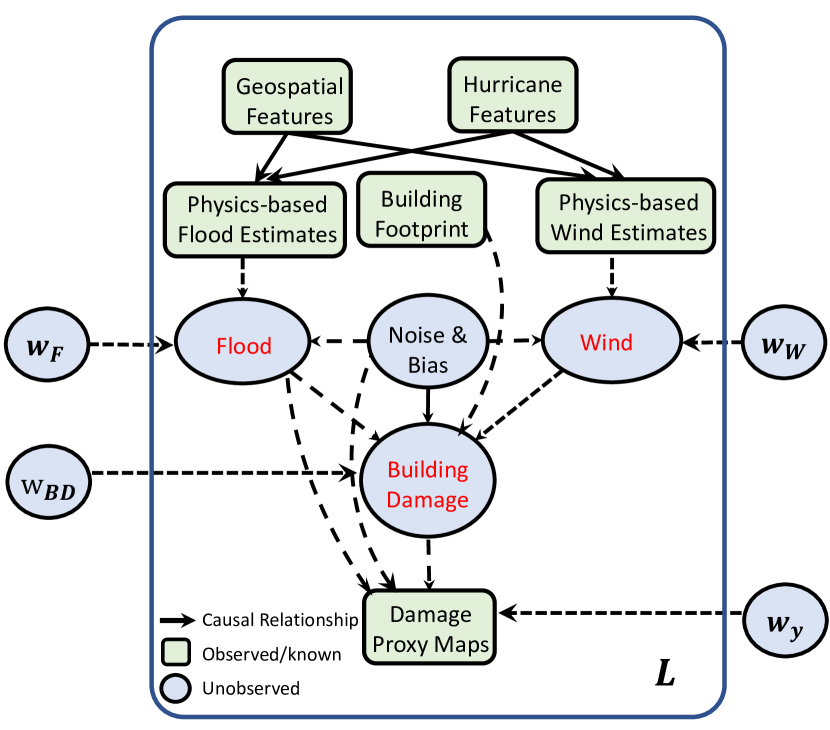
Figure 1. Overview of hurricane damage chain

2.1. Causal Bayesian Network Formulation for Hurricane Damage Chain

To rigorously evaluate how hurricanes impact building integrity via secondary hazards like flooding and wind, we’ve devised a causal Bayesian network, shown in Figure 1. This network integrates known variables, such as physics-based hazard models and building plans, with unobserved factors like the extent of flooding and building damage. The objective is to infer these latent variables using the network’s causal links. Crucially, each edge in our model represents a causal, not merely correlational, relationship. We begin by mathematically formalizing these elements, converting the conceptual framework into a structured probabilistic model.

2.1.1. Node variables modeling

We designate our unobserved variables, or feature vertices, as Flood and Wind, symbolized by $x_{F}$ and $x_{W}$, respectively. According to prior research (Paleo-Torres et al., 2020; Masoomi et al., 2019), these variables are continuous and follow a lognormal distribution. Building Damage is denoted as $x_{BD}$ and treated as a binary variable, where 1 indicates severe damage or complete destruction, and 0 implies minor or no damage.Each unobserved variable $x_{i}$ belongs to the set $X$, where $i\in\{W,F,BD\}$. The parent nodes for each $x_{i}$ are contained in the set $\mathcal{P}(i)$, pre-defined based on our understanding of the causal chain. We incorporate prior estimates $a_{W}$ and $a_{F}$ for wind and flooding, derived from geospatial models built on geophysical domain knowledge. Parent nodes for any sensed observations $X$ are denoted as $\mathcal{P}(x)$. A constant ”leak node,” $x_{0i}=1$, ensures child node activity even when other parents are inactive. The Disaster Proxy Map (DPM) encapsulates the impact of multi-hazard events. Interferometric Synthetic Aperture Radar (InSAR) captures elevation changes, indicated by $y>0$ in the DPMs. We also assume the existence of environmental noises $\epsilon_{y}$ and $\epsilon_{i},i\in\{W,F,BD\}$, following a standard normal distribution.

2.1.2. Causal dependency modeling

After defining the variables, it’s essential to parameterize their dependencies, or the edges connecting nodes. We use $w_{ji}$ ($j\in\mathcal{P}(i)$) to represent the weight of a parent node’s influence on its child node. For instance, the set of weights $w_{F}$ for the Flood node incorporates the weights defining causality from its parent nodes, such as $w_{aF}$, $w_{\epsilon_{F}}$, and $w_{0F}$.

For observed variable $y$, we assume its mapping function from parent nodes $\mathcal{P}(y)$ is lognormal (LN), represented as:

(1) $$\log y=\sum_{k\in\mathcal{P}(y)}w_{ky}x_{k}+w_{\epsilon_{y}}\epsilon_{y}+w_{0y}$$

Here, $\mathcal{P}(y)=\{x_{F},x_{BD},\epsilon_{y},x_{0}\}$.

For unobserved root variables $i\in\{W,F\}$, their parent nodes include prior estimates $a_{i}$, environmental noises $\epsilon_{i}$, and the leak node $x_{0}$. Their mapping function is:

(2) $$\log x_{i}=\sum_{k\in\mathcal{P}(i)}w_{ki}x_{k}+w_{\epsilon_{i}}\epsilon_{i}+w_{0i}$$

This aligns with our assumption that $x_{F}$ and $x_{W}$ follow a lognormal distribution.

For Building Damage ($i=BD$), $\mathcal{P}(BD)=\{x_{F},x_{W}\}$, and its activation function is:

(3) $$\log\frac{p(x_{i}=1|\mathcal{P}(i),\epsilon_{i})}{1-p(x_{i}=1|\mathcal{P}(i),\epsilon_{i})}=\sum_{k\in\mathcal{P}(i)}w_{k,i}x_{k}+w_{\epsilon_{i}}\epsilon_{i}+w_{0i}.$$

Given that the causal coefficients (represented by dashed arrows in Figure 1) and unobserved variables (blue circles) are unknown, the challenge lies in inferring this complex multi-layer Bayesian network, which combines unknown continuous and discrete variables along with uncertain dependency parameters.

2.2. Stochastic Variational Inference

After constructing the Bayesian network, we face two main challenges: the unknown parameters for causal dependencies and hazard distributions, and computational constraints for high-resolution mapping of large areas. To overcome this, we implement variational inference. This computational technique allows us to factorize the Bayesian network and approximate the posterior distributions of unobserved variables, such as building damage and secondary hazards, by maximizing the log-likelihood of the observed data. To ensure the method’s scalability, we execute the inference on a small, randomly selected batch of locations during each iteration. This balances computational efficiency with the need for comprehensive spatial analysis. The core objective of the variational inference is to derive and maximize a tight lower bound on the log-likelihood, which is formulated as a function of both the posteriors of unobserved variables and the causal weights. This approach effectively translates the theoretical Bayesian network into a practical, computationally efficient mechanism for large-scale hazard assessment. Accordingly, we derive the variational lower bound is :

(4) $$\begin{split}\log p(Y)&\geq\sum_{l\in N}\{\underbrace{\mathbb{E}_{q(X^{l},\epsilon^{l})}[\log p(y^{l},X^{l},\epsilon^{l})]}_{[1]}-\underbrace{\mathbb{E}_{q(X^{l},\epsilon^{l})}[\log q(X^{l},\epsilon^{l})]}_{[2]}\}\end{split}$$

where $q$ is the posteriors of all unknown variables.

To further obtain the explicit form of the final variational bound, we expand the item[1] as:

(5) $$\begin{split}&\mathbb{E}_{q(X^{l},\epsilon^{l})}[\log p(y^{l},X^{l},\epsilon^{l})]\\ &=\underbrace{\mathbb{E}[\log p(y|\mathcal{P}(y),\epsilon_{y})]}_{[3]}+\underbrace{\sum_{i}\mathbb{E}[\log p(x_{i}|\epsilon_{i},\mathcal{P}(i))]}_{[4]}\\ &+\underbrace{\sum_{i}\mathbb{E}[\log p(\epsilon_{i})]+\mathbb{E}[\log p(\epsilon_{y})]}_{C_{1}}\end{split}$$

Since $y|\mathcal{P}(y)\sim LN(\sum_{k\in\mathcal{P}(y)}w_{ky}x_{k}+w_{0y},w_{\epsilon_{y}}^{2})$, where $\mathcal{P}(y)=\{F,BD\}$. So we can calculate item[3]:

(6) $$\begin{split}&\mathbb{E}[\log p(y|\mathcal{P}(y),\epsilon_{y})]\\ &=-\log y-\log|w_{\epsilon_{y}}|-\frac{(\log y)^{2}+w_{0y}^{2}-2w_{0y}\log y}{2w_{\epsilon_{y}}^{2}}\\ &+\frac{\sum_{k\in\mathcal{P}(y)}w_{ky}^{2}\mathbb{E}(x_{k}^{2})+2(w_{0y}-\log y)\sum_{k\in\mathcal{P}(y)}w_{ky}\mathbb{E}(x_{k})}{2w_{\epsilon_{y}}^{2}}\end{split}$$

where $k=F$: $E(x_{k})=\exp(\mu_{k}+\sigma^{2}/2)$ and $E(x_{k}^{2})=(\exp(\sigma^{2})-1)\exp(2\mu_{k}+\sigma^{2})+\exp(\sigma^{2}+2\mu_{k})$. ; For $k=BD\}$, $\mathbb{E}(x_{i})=q_{k},\mathbb{E}(x_{i}^{2})=q_{k}$.

For the item[4], It should be derived separately because the $i\in\{W,F\}$ and $i\in\{SD,RD\}$ are different situations here, so the equation could be expanded first into:$\sum_{i}\mathbb{E}[\log p(x_{i}|\epsilon_{i},\mathcal{P}(i))]=\sum_{i\in\{W,F\}}\mathbb{E}[\log p(x_{i}|\epsilon_{i},\mathcal{P}(i))]+\sum_{i\in\{RD,BD\}}\mathbb{E}[\log p(x_{i}|\epsilon_{i},\mathcal{P}(i))]$ Then based on this equation, we could divide the equation into two different scenarios.

When the unobserved variable is continuous, we will derive the $\mathbb{E}[\log p(x_{i}|\epsilon_{i},\mathcal{P}(i))]$ for $i\in\{W,F\}$. Since $x_{i}|\epsilon_{i}$ follows a lognormal distribution, then $\log x_{i}|\epsilon_{i}$ follows a normal distribution. Then we could get the item[4] for $i\in\{W,F\}$:

(7) $$\mathbb{E}[\log p(x_{i}|\epsilon_{i},\mathcal{P}(i))]=-(w_{a_{i}}a_{i}+w_{0i})-\log|w_{\epsilon_{i}}|$$

When an unobserved variable $i$ is discrete, for example, a binary distribution, we can determine the result of $\mathbb{E}(\log p(x_{i}=m_{i}|\mathcal{P}(i),\epsilon_{i}))$ for $i\in\{BD\}$. The computation of item[4] for $i\in\{BD\}$ is :

(8) $$\begin{split}&\mathbb{E}(\log p(x_{i}|\mathcal{P}(i),\epsilon_{i}))\\ &=q_{i}\mathbb{E}(-\log[1+\exp(-w_{\epsilon_{i}}\epsilon_{i}-w_{0i}-\sum_{k\in\mathbf{P}(i)}w_{ki}x_{k})])\\ &+(1-q_{i})\mathbb{E}(-\log[1+\exp(w_{\epsilon_{i}}\epsilon_{i}+w_{0i}+\sum_{k\in\mathbf{P}(i)}w_{ki}x_{k})]).\end{split}$$

However, the distribution of $-\log[1+\exp(w_{\epsilon_{i}}\epsilon_{i}+w_{0i}+\sum_{k\in\mathbf{P}(i)}w_{ki}x_{k})$ is intractable as it is a log-sum-exp of mixing a series of discrete variables and continuous variables. Therefore, we need to get a tight lower bound of its expectation. Here without the loss of generality, we start from the case where $i$ has a single active parent.

With multivariate Taylor expansion, we can apply the standard quadratic bound for $\text{log}(1+\text{exp})$ (Jaakkola and Jordan, 1997):

$$\text{log}(1+e^{z})\leq g(\gamma)(z^{2}-\gamma^{2})+\frac{z-\gamma}{2}+\text{log}(1+e^{\gamma})$$

where $\gamma\in(0,\infty),g(\gamma)=\frac{1}{2\gamma}[\frac{1}{1+e^{-\gamma}}-\frac{1}{2}]$. Thus, we can obtain the lower bound as:

$$\begin{split}&\mathbb{E}(\log p(x_{i}|\mathcal{P}(i),\epsilon_{i}))\\ &\geq(1-q_{i})\mathbb{E}(z_{i})-\{g(\gamma_{i})(\mathbb{E}(z_{i}^{2})-\gamma_{i}^{2})+\frac{\mathbb{E}(z)-\gamma_{i}}{2}+\log(1+e^{\gamma_{i}})\}\end{split}$$

where

(9) $$\begin{split}&\mathbb{E}(z)=\sum_{k\in\mathcal{P}(i)}w_{ki}\mathbb{E}(x_{k})+w_{0i}\\ &\mathbb{E}(z^{2})=\sum_{k\in\mathcal{P}(i)}w_{ki}^{2}\mathbb{E}(x_{k}^{2})+w_{\epsilon_{i}}^{2}+w_{0i}^{2}+2w_{0i}\sum_{k\in\mathcal{P}(i)}w_{ki}\mathbb{E}(x_{k})\\ &+\sum\limits_{\begin{subarray}{c}r,s\in\mathcal{P}(i)\\ r\neq s\end{subarray}}w_{ri}w_{si}\mathbb{E}(x_{r})\mathbb{E}(x_{s})\end{split}$$

It is noted that for $k\in\{W,F\}$, as they are leaf nodes with all parent nodes known, and we postulate that $x_{k}$ follows a lognormal posterior with parameters of $\mu_{k}$ and $\sigma_{k}$, there is $\mathbb{E}(x_{k})=\exp(\mu_{k}+\sigma^{2}/2)$ and $\mathbb{E}(x_{k}^{2})=(\exp(\sigma^{2})-1)\exp(2\mu_{k}+\sigma^{2})+\exp(\sigma^{2}+2\mu_{k})$. After we finish the all the calculation form the item[1], we further move to derive the expansion of the item[2] as:

(10) $$\begin{split}\mathbb{E}_{q(X^{l},\epsilon^{l})}[\log q(X^{l},\epsilon^{l})]&=\sum_{i\in\{\}}q_{i}\log q_{i}+(1-q_{i})\log(1-q_{i})\\ &-\sum_{i\in\{F,W\}}[\mu_{i}+\log\sigma_{i}]+C_{2}.\end{split}$$

where $C_{2}$ is a fixed constant.

With the derivation of a tight variational lower bound for our causal Bayesian network focused on hurricane-induced hazards and damage, we proceed to optimize both unobserved variable posteriors and causal coefficients. Utilizing an Expectation-Maximization (EM) framework, the expectation step involves formulating closed-form update equations for the posteriors of wind (W), flood (F), and building damage (BD) by setting the gradients of the lower bound to zero. During the maximization phase, we employ Stochastic Gradient Descent (SGD) with mini-batches of randomly sampled data points from diverse locations. We’ve customized Stochastic Variational Inference to fast-track computation across expansive, high-resolution maps. In this, edge weights for the next iteration $t+1$ are updated as follows:

(11) $$\textbf{w}_{(t+1)}=\textbf{w}_{(t)}+\rho A\nabla\mathcal{L}(\textbf{w})$$

where $\rho$ adjusts the learning rate and $A$, serving as a preconditioner, is configured as the identity matrix to encourage model convergence.

Local pruning strategy for computational efficiency: To address computational challenges in large-scale mapping, we’ve created a local pruning strategy for our causal graph. Based on the sparsity of the real-world casual graph, we remove inactive nodes—like those for building damage in a location without any building footprints —while keeping crucial active nodes for parameter updates.

3. A Case Study of Hurricane Ian

The 2022 Hurricane Ian (Kijewski-Correa et al., 2023) is chosen as the case study. This section introduces the background of Hurricane Ian, and provides a detailed description of street-view imagery data collection, data pre-processing and damage level annotation.

3.1. Background of Hurricane Ian

On September 28, 2022, Hurricane Ian struck Lee County, FL, displacing over 130,000 residents and causing extensive coastal erosion. Our study involved capturing street-view images of 2,472 affected buildings from both StEER’s Hurricane Ian Response and our own field investigations. Utilizing StEER’s FAST handbook(Kijewski-Correa et al., 2019), two expert annotators classified the exterior damage into five levels, from 0 (no or minor damage) to 4 (destroyed). Statistical tests indicated high inter-coder reliability, with a Krippendorff’s alpha of 0.86 and a correlation coefficient of 0.97 (p ¡ 0.001). The final dataset revealed 6.1% of buildings suffered severe-to-total damage, 72.2% had no visible damage, and the remaining 27.8% were damaged.

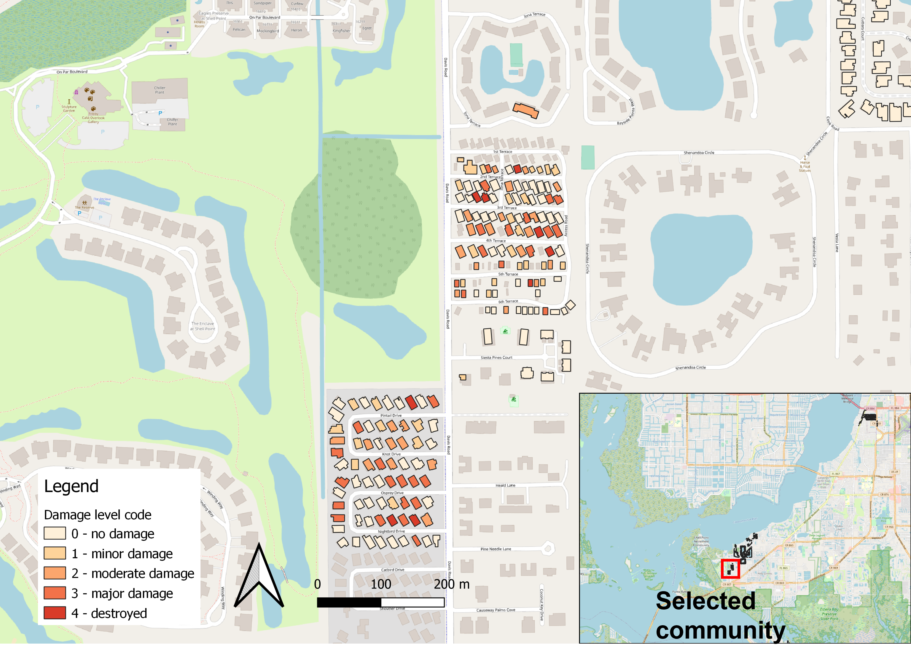
Figure 2. An example of damage level-labeled parcels in a selected community

3.2. Datasets and Evaluation

Our framework, depicted in Figure 1, heavily relies on three key inputs for inference: Wind Map, Flood Map, and Damage Proxy Map. Crafted by NIST and ARA, the Wind Map employs advanced simulations to detail peak and sustained winds. The Flood Map, produced via the CH3D-SWAN model(Sheng et al., 2010), offers storm surge simulations in Florida counties with a 20-meter grid granularity, and it is calibrated with hurricane Ian’s wind data(Peter Sheng et al., 2022). Meanwhile, the Damage Proxy Map (DPM) is a crucial contribution from NASA’s ARIA team, showcased in Fig. 3. Derived from Copernicus Sentinel-1 SAR images(ARIA, 2022), the DPM provides reliable, cloud-penetrant data in an 85 by 76 kilometer area around Fort Myers. Leveraging InSAR technology, the DPM serves as a foundational grid for rasterizing our datasets.

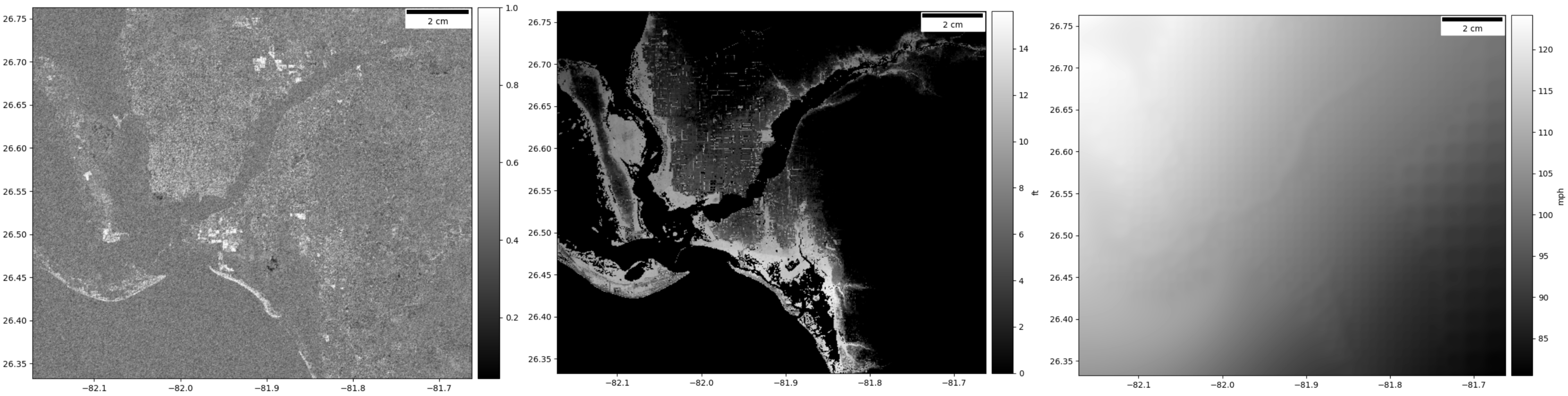
Figure 3. Overview of the DPM, Flood Map and Wind Map in Lee County, FL (from left to right)

In our study, we use the Receiver Operating Characteristic (ROC) curve and its Area Under the Curve (AUC) for evaluation. The ROC curve plots True Positive Rate (TPR) against False Positive Rate (FPR). A high AUC near 1 signifies strong model separability in identifying true damages versus false predictions. We set a threshold to categorize outcomes as ”damage exists” or ”no damage,” allowing for practical performance comparison. The ROC curve offers a balanced assessment over varied thresholds from 0 to 1.

3.3. Benchmarks

We evaluate our framework against three types of benchmark methods: Optical Imagery-Based Models, Fragility Curve-Based Models, and Direct DPM-Based Models. These benchmarks offer comprehensive comparisons to traditional approaches in post-hurricane building damage detection.

Optical Imagery-Based Models: We employ two top-performing models from the xView2 Challenge as baselines: FCS-Net(Khvedchenya and Gabruseva, 2021) and Dual-HRNet. FCS-Net uses a Siamese architecture with ResNet34(He et al., 2015) and U-Net (Ronneberger et al., 2015)components, while Dual-HRNet integrates two HRNets (Wang et al., 2020; Sun et al., 2019) with serveral fusion blocks. We first test these pre-trained models on our datasets without fine-tuning, and then fine-tune them for further evaluation. The results are summarized in Table 1.

Fragility Curves: We leverage a fragility curve model developed by Andres Paleo-Torres et al.(Paleo-Torres et al., 2020), focusing on the vulnerability of Florida’s residential buildings to coastal flooding. It adapts tsunami fragility functions and outlines six damage states, offering a tailored benchmark to measure hurricane-induced building vulnerability in Florida.

3.4. Results

In this section, we present the results derived from our model and draw comparisons with conventional methodologies, including the flood-map-based model, DPM-based model, and optical imagery-based models. This comparative analysis offers a clear understanding of our model’s performance, highlighting its advantages and potential improvements over traditional techniques.

3.4.1. Result analysis

Our model excels in key performance metrics, making it a compelling alternative to more traditional, label-dependent methods. With a True Positive Rate (TPR) of 0.8293 and an Area Under the Curve (AUC) score of 0.7553, it surpasses other models in the landscape. While its True Negative Rate (TNR) of 0.6221 may not be the highest, it is nonetheless a competitive figure. Importantly, the model obviates the need for ground-truth labels, a feature that greatly simplifies the training process and saves significant time and resources. This is especially advantageous in scenarios where label acquisition is cumbersome or not feasible.

Compared to this, the fine-tuned Dual-HRNet model, which necessitates labels for training, produced TPR and TNR scores of 0.8217 and 0.6251, respectively—figures that are closely matched but not exceeding ours. Other benchmark models, such as the Pure DPM-based Estimation and the Fragility Curve-based Estimation, lagged behind in both TPR and TNR. Additionally, the fact that our model performs robustly without requiring additional flood or wind maps highlights its adaptability and widens its applicability. Therefore, our model not only streamlines the training process but also demonstrates that label-free, efficient training can yield results on par with more resource-intensive approaches.

Table 1. Comparison of TPR, TNR, and AUC of our model and baselines. Note that (1) our probabilistic model that fuses DPMs and physics-based flood and wind model does not require any labels in training stage, (2) FCS-Net and Dual-HRNet are computer vision models using optical satellite imagery and pretrained in historical events. ”w/o finetuning” means the model is directly adopted to estimate building damage, which is equivalent to our model setup, ”finetuned” means the model is finetuned using labeled building damage datasets for Hurricane Ian. The results show that our model that does not require any labeled data achieves comparable performance as the model finetuned on labeled data. NA means Not Available, meaning AUC is not calculated for deterministic models like FCS-Net and Dual-HRNet.

Model	TPR	TNR	AUC
Our model (w/o label training)	0.8293	0.6221	0.7553
FCS-Net (w/o finetuning)	0.2713	0.8941	NA
FCS-Net (w/ finetuning)	0.2098	0.9386	NA
Dual-HRNet (w/o finetuning)	0.0912	0.9795	NA
Dual-HRNet (w/ finetuning)	0.8217	0.6251	NA
DPM-based Model (w/o label training)	0.6498	0.6249	0.6739
Fragility Curve (w/o label training)	0.5669	0.6246	0.5695

3.4.2. Ablation Study

Our ablation study yielded key insights into the interplay between different components and parameters in our model. First, we noted that batch size has a marked influence on both computational time and model performance, as evidenced by Table 2. Specifically, increasing the batch size from 128 to 1024 slashed computational time from 5812 to 941 seconds but resulted in a modest performance decline, as AUC dropped from 0.7553 to 0.7311. This highlights a trade-off between computational speed and predictive accuracy. Second, we assessed the contributions of Variational Inference (VI) and Pruning strategies, as outlined in Table 3. VI Full exhibited the best performance with an AUC of 0.7825 and a Variational Lower Bound (VLB) of 1.1442, outperforming the worst performer, MCMC Local, which posted an AUC of 0.7117 and a VLB of 0.7140. This stark contrast substantiates the superiority of VI methods over MCMC methods. Further, within both VI and MCMC categories, the Local Pruned Graph yielded slightly lower AUC but better VLB, suggesting it offers a tighter lower bound at a minimal AUC cost. Thus, our ablation study not only quantifies the impact of batch size and computational techniques but also validates the strategic choices made in our model’s architecture.

Table 2. The computational time for different batch sizes.

Batch size $m$	128	256	512	1024
AUC	0.7553	0.7553	0.7329	0.7311
Time used (second)	5812	2729	1267	941

Table 3. Evaluation of the effectiveness of Variational Inference and Prunning strategy in our framework. We present AUC values and variational lower bound (VLB).

Method	AUC	VLB
VI Full	0.7825	1.1442
VI Local	0.7553	1.1249
MCMC Full	0.7271	0.7797
MCMC Local	0.7117	0.7140

4. Discussion and Conclusion

This paper unveils a novel deep learning model that uses a causal Bayesian network to quickly assess building damage post-hurricane using InSAR imagery. Tested on Hurricane Ian, our model outperforms both state-of-the-art optical imagery benchmarks and traditional methods, all without requiring ground-truth labels for rapid deployment post-disaster.

The strength of our model lies in its causal graph, which simulates real-world hurricane-induced hazards leading to building damage, unlike previous models that merely map noisy remote sensing data to damage outcomes. This allows for the effective fusion of physics-based flood and wind estimates with sensor data, enhancing accuracy and speed of assessments. However, existing optical imagery models like FCS-Net and Dual-HRNet falter when applied to new events, demonstrating poor generalizability and low True Positive Rates (Table 1). Fine-tuning these models presents logistical hurdles, primarily the need for labor-intensive ground-truth labeling, limiting their usefulness in rapid damage assessments.

While promising, our model does have limitations, particularly in areas with steep slopes that can interfere with SAR backscatter. Future work should consider integrating InSAR with optical imagery for a more comprehensive and accurate damage assessment.

- (1)
- ARIA (2022) NASA-JPL/Caltech ARIA. 2022. Damage Proxy Map (DPM) for Hurricane Ian using Copernicus Sentinel-1 data. Available at: http://aria-share.jpl.nasa.gov/.
- Barras (2007) John A Barras. 2007. Satellite images and aerial photographs of the effects of Hurricanes Katrina and Rita on coastal Louisiana. Technical Report. Geological Survey (US).
- Berezina and Liu (2022) Polina Berezina and Desheng Liu. 2022. Hurricane damage assessment using coupled convolutional neural networks: a case study of hurricane Michael. Geomatics, Natural Hazards and Risk 13, 1 (2022), 414–431.
- Calton and Wei (2022) Landon Calton and Zhangping Wei. 2022. Using artificial neural network models to assess hurricane damage through transfer learning. Applied Sciences 12, 3 (2022), 1466.
- He et al. (2015) Kaiming He, Xiangyu Zhang, Shaoqing Ren, and Jian Sun. 2015. Deep Residual Learning for Image Recognition. arXiv:1512.03385 [cs.CV]
- Jaakkola and Jordan (1997) Tommi S Jaakkola and Michael I Jordan. 1997. A variational approach to Bayesian logistic regression models and their extensions. In Sixth International Workshop on Artificial Intelligence and Statistics. PMLR, 283–294.
- Khvedchenya and Gabruseva (2021) Eugene Khvedchenya and Tatiana Gabruseva. 2021. Fully convolutional Siamese neural networks for buildings damage assessment from satellite images. arXiv:2111.00508 [cs.CV]
- Kijewski-Correa et al. (2019) T Kijewski-Correa, K Mosalam, DO Prevatt, I Robertson, and D Roueche. 2019. Field assessment structural team (FAST) Handbook, Version 1.2. Structural Engineering Extreme Events Reconnaissance (2019).
- Kijewski-Correa et al. (2023) Tracy Kijewski-Correa, David Prevatt, David Roueche, Ian Robertson, Mohammad Alam, Amir Safiey, Ioannis Zisis, Oscar Lafontaine, Omar Nofal, Landolf Rhode-Barbarigos, Arthriya Subgranon, Dylan Faraone, Jonathon Micali, Jorge X Santiago-Hernández, and Duzgun Agdas. 2023. StEER: Hurricane Ian Early Access Reconnaissance Report (EARR). https://doi.org/10.17603/DS2-3PC2-7P82
- Lee (2005) SARO Lee. 2005. Application of logistic regression model and its validation for landslide susceptibility mapping using GIS and remote sensing data. International Journal of remote sensing 26, 7 (2005), 1477–1491.
- Lin et al. (2021) Chen Lin, Yundong Li, Yi Liu, Xiang Wang, and Shuo Geng. 2021. Building damage assessment from post-hurricane imageries using unsupervised domain adaptation with enhanced feature discrimination. IEEE Transactions on Geoscience and Remote Sensing 60 (2021), 1–10.
- Masoomi et al. (2019) Hassan Masoomi, John W van de Lindt, Mohammad R Ameri, Trung Q Do, and Bret M Webb. 2019. Combined wind-wave-surge hurricane-induced damage prediction for buildings. Journal of Structural Engineering 145, 1 (2019), 04018227.
- Paleo-Torres et al. (2020) Andres Paleo-Torres, Kurtis Gurley, Jean-Paul Pinelli, Mohammad Baradaranshoraka, Mingwei Zhao, Anawat Suppasri, and Xinlai Peng. 2020. Vulnerability of Florida residential structures to hurricane induced coastal flood. Engineering structures 220 (2020), 111004.
- Peter Sheng et al. (2022) Y Peter Sheng, Vladimir A Paramygin, Kun Yang, and Adail A Rivera-Nieves. 2022. A sensitivity study of rising compound coastal inundation over large flood plains in a changing climate. Scientific Reports 12, 1 (2022), 3403.
- Ronneberger et al. (2015) Olaf Ronneberger, Philipp Fischer, and Thomas Brox. 2015. U-Net: Convolutional Networks for Biomedical Image Segmentation. arXiv:1505.04597 [cs.CV]
- Sheng et al. (2010) Y Peter Sheng, Vadim Alymov, and Vladimir A Paramygin. 2010. Simulation of storm surge, wave, currents, and inundation in the Outer Banks and Chesapeake Bay during Hurricane Isabel in 2003: The importance of waves. Journal of Geophysical Research: Oceans 115, C4 (2010).
- Smith (2021) A Smith. 2021. US billion-dollar weather and climate disasters in historical context (NOAA national centers for environmental information). (2021).
- Structural Extreme Events Reconnaissance (2023) (StEER) Structural Extreme Events Reconnaissance (StEER). 2023. Hurricane Ian Street View Comparison. Available online. https://d19lqd7ccqm7zl.cloudfront.net/compare/index.html Accessed on June 20, 2023.
- Sun et al. (2019) Ke Sun, Yang Zhao, Borui Jiang, Tianheng Cheng, Bin Xiao, Dong Liu, Yadong Mu, Xinggang Wang, Wenyu Liu, and Jingdong Wang. 2019. High-Resolution Representations for Labeling Pixels and Regions. arXiv:1904.04514 [cs.CV]
- Wang et al. (2022) Hao Wang, Chao Tao, Ji Qi, Rong Xiao, and Haifeng Li. 2022. Avoiding Negative Transfer for Semantic Segmentation of Remote Sensing Images. IEEE Transactions on Geoscience and Remote Sensing 60 (2022), 1–15.
- Wang et al. (2020) Jingdong Wang, Ke Sun, Tianheng Cheng, Borui Jiang, Chaorui Deng, Yang Zhao, Dong Liu, Yadong Mu, Mingkui Tan, Xinggang Wang, Wenyu Liu, and Bin Xiao. 2020. Deep High-Resolution Representation Learning for Visual Recognition. arXiv:1908.07919 [cs.CV]
- Xu et al. (2022) Susu Xu, Joshua Dimasaka, David J Wald, and Hae Young Noh. 2022. Seismic multi-hazard and impact estimation via causal inference from satellite imagery. Nature Communications 13, 1 (2022), 7793.
- Zhai and Peng (2020) Wei Zhai and Zhong-Ren Peng. 2020. Damage assessment using google street view: Evidence from hurricane Michael in Mexico beach, Florida. Applied geography 123 (2020), 102252.
- Zhao and Lu (2018) Chaoying Zhao and Zhong Lu. 2018. Remote sensing of landslides—A review. Remote Sensing 10, 2 (2018), 279.