Analytic solutions for irregular diffusion equations with concentration dependent diffusion coefficients

Abstract

We investigate diffusion equations which have concentration dependent diffusion coefficients with physically two relevant Ansätze, the self-similar and the traveling wave Ansatz. We found that for power-law concentration dependence some of the results can be expressed with a general analytic implicit formulas for both trial functions. For the self-similar case some of the solutions can be given with a formula containing the hypergeometric function. For the traveling wave case different analytic formulas are given for different exponents. For some physically reasonable parameter sets the direct solutions are given and analyzed in details.

1 Introduction

The simplest mass or energy transfer is diffusion or heat conduction phenomena which is one of the most important mass transport phenomena in nature therefore it has an enormous interest in science and engineering as well. The corresponding literature has grown enormously over the past 200 years. Without completeness we just mention some recent textbooks [1, 2, 3, 4].

The simplest diffusion process is the regular one, which is formulated with well-known parabolic partial differential equation (PDE) in the form of

$$\frac{\partial C(x,t)}{\partial t}=D\cdot\Delta C(x,t),$$ (1)

where $C(x,t)$ is the concentration an D is the diffusion coefficient which is a positive real constant and $\Delta$ represents the Laplace differential operator in arbitrary dimensions in arbitrary coordinate system. Certain boundary conditions belong to equation (1). There are definite solutions for finite systems, which often are related to engineering applications [5, 6].

There are numerous works done in the last decades to find analytic solutions beyond the well-known Gaussian and error functions. The best known is the work of Bluman and Cole [7] from 1969 who gave an analysis based on a general symmetry analysis method giving numerous analytic solutions, some of them are expressible with Gaussian or error functions. As we see they did not present any kind of solutions which looks similar to ours (and which we present in the following).

In case of infinite horizon the fundamental solution is the Gaussian function which has application in different areas of science. In the last year we found additional, physically relevant solutions with the help of the self-similar Ansatz [14, 15] which are a logical generalization of the fundamental solution. These solutions are the multiplication of the Gaussian function and the Kummer’s M and Kumer’s U functions which have an additional free parameter, due to this parameter even decaying and oscillatory solutions can be given. The applied self-similar Ansatz will be defined later on in this study in all details. The diffusion coefficient in certain cases may be considered constant, however there are cases where it may vary [8]. For two dimensional models important results have been obtained in ref.[9] and for a diffusive-reactive case in ref.[10]. Environmental aspects of diffusive very fine particles is discussed in [11].

Diffusion on surfaces is also a significant topic, with possible irregular features [12]. The chaotic properties of this latter system have been studied in [13].

The general form of diffusion equation comes from a conservation law and reads,

$$\frac{\partial C}{\partial t}=\frac{\partial}{\partial x}\left(D\frac{\partial C}{\partial x}\right).$$ (2)

In case the diffusion coefficient $D$ depends on parameter $C$, then in general it will also depend on $x$. So the case $D(C[x,t])$ is possible. The diffusion coefficient may depend on certain physical quantities, and it may vary depending in which phase the system is: gaseous, fluid or solid phase. In this sense there is a difference between the dependence of mass diffusion coefficient and heat diffusion coefficient dependence on the parameter $C$. The $C$ stands for the density or concentration in case of mass diffusion and $C$ corresponds to temperature in case of heat diffusion.

The investigation of the regular diffusion is just the first step to understand diffusion process in general, however there are much more complex and difficult diffusion processes in nature. The diffusion coefficient can have additional dependencies like, time, space of even a tricky combination of both. (We examined the case when the diffusion coefficient depend on the function $x/t^{\frac{1}{2}}$) In the last years we systematically investigated of such equations and gave new self-similar solutions together with detailed numerical investigations as well. We applied explicit, semi-explicit and implicit numerical schemes to solve numerically the corresponding PDEs and compared the evaluated solutions to the exact mathematical ones [16, 17, 18]. We found that in most cases the leapfrog-hopscotch method is the most expedient method to solve PDEs. These kind of diffusion equations with time, space and "time-and-space" dependent diffusion coefficients do have analytic solutions with the similar structure the fundamental Gaussian solution multiplied by the Kummer’s M and Kummer’s U functions or with the Whittaker type functions. Due to the extra free parameter different type of decaying solutions are always exist with different asymptotics. Some solutions have additional oscillations as well.

On this way we may go a bit further and ask the question what are the properties of the diffusion process when the diffusion coefficient directly depend on the concentration, in the form of $D(C[x,t])$. These cases cover certain real non-linear diffusion processes described with highly non-linear PDEs. In the following we will investigate this question in details.

2 Theory and Results

It is evident that diffusion is in general a three dimensional process beyond Cartesian symmetry, however we limit our analysis to a single Cartesian space dependent equation. In case we consider the equation of heat transfer, then we have for the heat flux $q=-\kappa T_{x}$, where $\kappa$ is the thermal conductivity. If $\kappa$ depends on temperature we have for the energy balance equation,

$$\rho c_{p}\frac{\partial T}{\partial t}=\frac{\partial}{\partial x}\left(\kappa(T)\cdot\frac{\partial T}{\partial x}\right).$$ (3)

The function of $\kappa(C[x,t])$ in principle can be any kind of continuous function with existing first derivative with respect to the concentration $C(x,t)$.

There are numerous studies available in which various the non-linear diffusion (or heat conduction) equations were solved with different methods and means and sometimes analytic solutions are given. Without completeness we cite the most relevant studies from the last seven decades.

We should start our reference with the work of Fujita [19] from 1952 who gave analytical solutions when the diffusion coefficient has the form of $D(C)=D(0)/(1-\lambda C)$.

Later Pattle [20] in 1959 gave solutions with compact support for diffusion from an instantaneous point source in one, two, or three dimensions. Philip [21] derived exact solutions for the non-linear diffusion equation when the concentration has the forms of $D(C)=D_{0}/(1-\lambda C),D(C)=D_{0}/(1-\lambda C)^{2}$ and $D(C)=D_{0}/(1+2aC+bC^{2})$.

Boyer [22] used a special kind of general self-similar Ansatz with the form of $T(x,t)=U(t)Y(r/R(t))$ and solved the non-linear heat conduction equation when the thermal conductivity was given in the form of $\kappa(T)=(\alpha+\beta T+\gamma T^{2})^{-1}$.

In 1964 Bankoff [23] investigated heat conduction or diffusion with change of phase and presented numerous methods how the solutions can be derived with series expansion or integral methods.

Knight and Philip [24] gave solution for the case of $D(C)=a(b-C)^{-2}$ with the help of the linearisation of the equation.

Tuck [25] solved the diffusion equation for $D(C)=kC^{n}$ with the constant source boundary condition with the self-similar solution and presented results with compact supports.

Munier et al. [26] presented that the self-similar and the partially invariant solutions are identical and introduced the theory of homology with new type of solutions. These are related through the Bäcklund transformation. They acknowledge in the paper, that for $n=-1$ is an exceptional case, where they met singularities. In this paper we discuss the case $n=-1$, and we give an explicit continuous solution.

King [27] solved a cylindrical symmetric non-linear diffusion equation with the self-similar Ansatz (which is very similar to our) and found solutions which can be expressed with the Airy functions.

Sadighi and Ganji [28] applied the variational iteration method and presented analytic results in form of final polynomials.

Hayek [29] presented an exact solution for a nonlinear diffusion equation in a radially symmetric n-dimensional case in inhomogeneous medium with the help of the self-similar Ansatz (Eq.6) which we also apply.

Kosov and Semenov [30] derived new radially symmetric exact solutions of the multidimensional nonlinear diffusion equation, which can be expressed in terms of elementary functions, Jacobi elliptic functions, Bessel functions, the exponential integral and the Lambert-W function.

Luckily to us, it must be strongly emphasized that we cannot identify solutions in the above cited literature which is exactly the same as our Eq. (16). Our personal problem with some of the mentioned studies that after doing the symmetry reduction the mathematical properties of derived ODEs are not investigated and the parameter dependence of the solutions are seldom discussed in details. We think that is the crucial point of the whole investigation and when that is properly done then much larger part of the scientific community (including applied physicists, chemist or various engineers) can directly profit from these solutions. We think that clear-cut well-explained analytic formulas still have high relevance in the understanding of physics.

As an outlook we mention some analytic studies of some non-linear reaction diffusion equations which are non-linear diffusion equations with one or more extra source terms.

An exhaustive group classification of such equation were evaluated by Dorodnitryn [31] in 1982.

The non-classical symmetry reduction was done by Arrigo et al. [32] in 1994.

Vijayakumar [33] presented a study in which he investigated the generalized diffusion equations (the Fisher, Newell-Whitehead and Fitzhugh-Nagumo equations) via the isovector approach and showed analytic results as well.

Cherniha and Serov [34] investigated the more general nonlinear diffusion equations with convection term with the Lie and non-Lie symmetry methods and presented additional solutions. However non clear-cut formulas are given with parameter studies.

Reductions and symmetries properties for a generalized Fisher equation with a diffusion term dependent on density and space was investigated by Chulian et al. [35].

Liu [36] gave a generalized symmetry classification, and gave the integrable properties with exact solutions for some nonlinear reaction-diffusion equations.

Qu et al. [37] applied the conditional Lie - Bäcklund symmetries with differential constraints and presented explicit solutions for a class of nonlinear reaction-diffusion equations.

It is important to mention here that this is just the simplest (the phenomenological) way to introduce non-linearity into the heat conduction equation. We still apply the Fourier law, where the heat flux is equal to the temperature gradient times thermal conductivity $q=-\kappa T_{x}$ which has now got an extra temperature dependence $\kappa(T)$. There is a mathematically more rigorous method to derive non-linear heat conduction equations which go beyond the Fourier law. The heat flux should be approximated with the higher temporal derivatives of the temperature. If the second term is considered we arrive to the Cattaneo-Vernotte equation [38, 39, 40], more on such kind of heat conduction equations can be found in the classical work of Gurtin and Pipkin [41] or in the work of Joseph and Preziosi [42]. Such heat conduction equations have finite signal propagation velocity properties. An Euler-Poisson-Darboux type of non-autonomous time-dependent heat conduction equation was derived by Barna and Kersner [43] which had solutions with a compact support. To describe heat pulse experiments "beyond the Cattaneo-Vernotte" models were applied bye Kovács and Ván [44].

Numerical investigation of Eq. (3) was done by [45] applying the implicit Euler method. In the following we will investigate this equation with the reduction mechanism applying two physically relevant trial functions, the self-similar and the traveling wave Ansätze. It is worth to mention here that this equation is a bit similar to the porous media equation which has the form of $U_{t}=\Delta(U^{m})$ where $m>1$ and was heavily investigated in former times [46, 47, 48]. We have to emphasise that if eq. (2) has an extra source than we arrive to further scientific fields as are the Fisher equation [50, 51], Turing model [52] or Swift - Hohenberg equation [53] for nonlinear optics. The diffusion equation has a wide range of applicability in science, which also includes the theory of pricing [54, 55].

After dividing by $\rho c_{p}$ equation (3) can be also written as a diffusion equation,

$$\frac{\partial T}{\partial t}=\frac{\partial}{\partial x}\left(D_{h}(T)\cdot\frac{\partial T}{\partial x}\right),$$ (4)

where $D_{h}=\kappa/(\rho c_{p})$ is the heat diffusion coefficient.

Because the heat and mass diffusion equation has the same PDE form, we simply consider the general dependence $D=\zeta(C)$ for (2), which corresponds to $D_{h}=\zeta(T)$ for (4) and we study the following equation:

$$\partial_{t}C=\zeta(C)_{C}\cdot C_{x}^{2}+\zeta(C)\cdot C_{xx},$$ (5)

where the subscripts mean the partial derivations, respectively. In the following we study the consequences of such dependence, when the diffusion may vary in terms of the parameter $C$.

2.1 Self-similar Analysis

Let’s start with the self-similar Ansatz [48, 49, 56] of the form of

$$C(x,t)=t^{-\alpha}f\left(\frac{x}{t^{\beta}}\right)=t^{-\alpha}f(\eta),$$ (6)

where $f(\eta)$ is the shape function with the reduced variable $\eta$, the two self-similar exponents $\alpha$ and $\beta$ are responsible for the decay and spreading of the solutions if both have non-negative values. In the last decade we generalized this kind of Ansatz to multiple spatial dimension and applied it to the Rayleigh-Bénard convection problems [57, 58] or to the heated boundary layer equations [59].

To make and in-depth analysis the functional form of the concentration dependent diffusion coefficient has to be defined. We start with the most evident case, the power law dependence:

$$\zeta(C[x,t])=a\cdot C(x,t)^{n}\hskip 14.22636pt\textrm{where n}\varepsilon\mathbb{R}$$ (7)

and the constant $a$ has to role to fix the dimension. (For simplicity we fix its numerical value to unity.)

If we insert this equation into (5) we get the following equation

$$\rho c_{p}\left(-\alpha t^{-\alpha-1}f-\beta\,t^{-\alpha-1}f^{\prime}\right)=nt^{-\alpha n-\alpha-2\beta}f^{\prime 2}+t^{-\alpha n-\alpha-2\beta}f^{\prime\prime},$$ (8)

where prime means derivation in respect to $\eta$.

After simplification with $t^{-\alpha}$ one arrives to:

$$\rho c_{p}\left(-\alpha t^{-1}f-\beta\,t^{-1}f^{\prime}\right)=nt^{-\alpha n-2\beta}f^{\prime 2}+t^{-\alpha n-2\beta}f^{\prime\prime}.$$ (9)

Both sides of the equation has the same decay in time if

$$-1=-n\alpha-2\beta,$$ (10)

or $\alpha=(1-2\beta)/n$.

After simplification with $t^{-1}$, and inserting the value of $\alpha$ in the equation, we arrive to the ordinary differential equation (ODE) of

$$\rho c_{p}\left(-\left[\frac{1-2\beta}{n}\right]f(\eta)-\beta\eta f(\eta)^{\prime}\right)=nf^{n-1}f^{\prime 2}+f^{n}f^{\prime\prime}.$$ (11)

Now we have to make case studies for different $n$s.

2.2 Case $n=0$

If $n=0$ we have the differential equation which corresponds to the usual diffusion equation, where the diffusion coefficient is constant. Although this is considered a relatively known case, here we present two very recent results for infinite horizon [60]. Beyond the usual Gaussian solution

$$C(x,t)=\frac{1}{\sqrt{t}}e^{-\frac{x^{2}}{4Dt}},$$ (12)

there are further relative simple solutions. There is a countable set of even solution relative to the spatial coordinate, the most simple one is (beyond Gaussian)

$$C(x,t)=\frac{1}{t^{\frac{3}{2}}}e^{-\frac{x^{2}}{4Dt}}\left(1-\frac{1}{2D}\frac{x^{2}}{t}\right).$$ (13)

There is also a countable set of odd solutions relative to the spatial coordinate, a simple one is

$$C(x,t)=\frac{x}{t^{\frac{5}{2}}}e^{-\frac{x^{2}}{4Dt}}\left(1-\frac{1}{6D}\frac{x^{2}}{t}\right).$$ (14)

2.3 Case $n\neq 0$

If $n\neq 0$ the equation (11) is more complex. Unlike the regular diffusion equation, we have now three parameters $\alpha,\beta$ and $n$ and two of them remains free, $\alpha=(1-2\beta)/n$. The solution has now the direct form of $C(x,t)=t^{\frac{1-2\beta}{n}}f(x/t^{\beta})$ The obtained ODE (11) has no general closed form solution for arbitrary $\beta$ and n. We will see that only for some special fixed $\beta$ and n combinations give us analytic results.

In the following case $n=-1$ will be considered with special attention, because corresponds to a characteristic dependence for dilute systems [8, 10].

2.3.1 Case $\beta=0$

We may start with the case of $\beta=0$ which give us an implicit solution of

$$\int^{f(\eta)}\pm\frac{na^{2n}(2+n)}{\sqrt{-na^{2n}(2+n)(2a^{2+n}\rho c_{p}-c_{1})}}da-\eta-c_{2}=0.$$ (15)

It turned out after some algebra, that if all four parameters of the integral $n,c_{1},\rho$ and $c_{p}$ are arbitrary rational numbers, there is a definite solution which can be expressed with the ${}_{2}F_{1}()$ hypergeometric function [61]

$$\left(n(n+2)f(\eta)^{1+2n}\sqrt{1-\frac{2\rho c_{p}f(\eta)^{2+n}}{c1}}\right)\times$$

$${}_{2}F_{1}\left(\frac{1}{2},\frac{1+n}{2+n};1+\frac{1+n}{2+n};\frac{2\rho c_{p}f(\eta)^{2+n}}{c_{1}}\right)\times$$

$$\left((1+n)\sqrt{-n(2+n)f(\eta)^{2n}[2\rho c_{p}f(\eta)^{2+n}-c1]}\right)^{-1}-$$

$$\eta-c_{2}=0.$$

(16)

Considering the more special case of $c_{1}=0$ the integral can be given in closed form for general $\rho c_{p}$ and $n$ values, so the implicit equation reads as follows:

$$\pm\frac{\sqrt{2}(2+n)f(\eta)^{1+2n}}{\sqrt{-nf(\eta)^{3n+2}(2+n)\rho c_{p}}}-\eta-c_{2}=0\,.$$ (17)

As we can see on this result, that in the denominator of the fraction, the argument of the square root is positive if for certain constraints. One of the possibilities is if $n$ is a negative number with small absolute value. We rise this latter equation to the second power and we get

$$f(\eta)^{n}=-\frac{n\rho c_{p}}{2(2+n)}(\eta+c_{2})^{2}.$$ (18)

For $n=-1$ both sides of the equation are positive

$$\frac{1}{f}=\frac{\rho c_{p}(\eta+2)^{2}}{2}.$$ (19)

This gives for the $C(x,t)$, in case $\alpha=(1-2\beta)/n=-1$:

$$C(x,t)=tf(\eta)=t\cdot\frac{2}{\rho c_{p}(x+c_{2})^{2}}.$$ (20)

One may arrive to this result by applying to equation (2), the standard change of variables $C(x,t)=A(t)\cdot B(t)$, for $n=-1$. This relation fulfils the equation (3), however it is divergent for large times.

2.3.2 Case $\beta=1$

For the second case let’s take $\beta=1$ and $n=-1$ with the solution of

$$f(\eta)=\frac{c_{1}^{2}}{-\rho c_{p}(1+c_{1}\eta)+c_{1}^{2}c_{2}e^{c_{1}\eta}},$$ (21)

It is clear that for the case $\rho c_{p}(1+c_{1}\eta)=c_{1}c_{1}^{2}e^{c_{1}\eta}$ the shape function becomes singular at one or two points where the linear equation is touches or intersects the exponential equation a nice example, when all four parameters have unit values. We exclude such non-physical solutions from our analysis. It is also clear that such solutions arise when the $\rho$ and $c_{p}$ are much larger than the initial conditions $c_{1}$ and $c_{2}$.

Figure (1) shows the solutions of Eq. (21) for the shape functions for two different parameter sets.

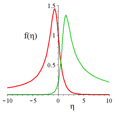
Figure 1: The solution of Eq. (21). The used parameter sets $\rho\cdot c_{p},c_{1},c_{2}$ for the red and green lines are $(1,1,2)$, and $(1,-2,5)$, respectively.

We analyze the function (21) by evaluating the derivative of it

$$\frac{\partial f}{\partial\eta}=\frac{c_{1}^{2}(\rho c_{p}c_{1}-c_{1}^{3}c_{2}e^{c_{1}\eta})}{(-\rho c_{p}(1+c_{1}\eta)+c_{1}^{2}c_{2}e^{c_{1}\eta})^{2}}.$$ (22)

As one can see, this function has an extreme value if

$$\rho c_{p}c_{1}=c_{1}^{3}c_{2}e^{c_{1}\eta}.$$ (23)

This means that this extrema will occur at the value of $\eta$

$$\eta_{*}=\frac{1}{c_{1}}\ln\frac{\rho c_{p}}{c_{1}^{2}c_{2}}.$$ (24)

One can see, that if

$$\rho c_{p} > c_{1}^{2}c_{2},\,\,\,\eta_{*}>0,$$ (25)

$$\rho c_{p} < c_{1}^{2}c_{2},\,\,\,\eta_{*}<0.$$ (26)

Figure (2) however presents the $C(x,t)$ total solution in the form of:

$$C(x,t)=\frac{1}{t}\left(\frac{c_{1}^{2}}{-c_{p}\rho(1+c_{1}\rho(x/t)+c_{1}^{2}c_{2}e^{\frac{c_{1}x}{t}}}\right).$$ (27)

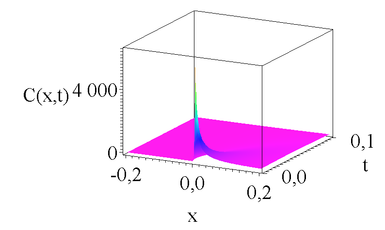
Figure 2: The solution of Eq. (27), the presented $C(x,t)$ function is for $\alpha=1,\beta=1,\rho=1,c_{p}=0.1,c_{1}=15,c_{2}=0.7,$ parameter set, respectively.

As a third mathematical case we found a solutions for the parameter pair of $\beta=-1/2$ and $n=-2$. Unfortunately, the result is a multi-valued implicit formula with real and complex parts. We tried to tune the parameters $c_{1},c_{2}$ and $\rho c_{p}$ but cannot found any solution which could be interpreted physically e.g. has some reasonable asymptotic for infinite time and space coordinates.

There are exotic but existing real materials which have temperature dependent heat conduction coefficients. As a first example we may mention magnetically aligned single wall carbon nanotube films [63] where the heat conduction coefficient has linear temperature dependence between 50 and 250 K. Our second example is bulk semiconductor at large temperature gradient. The authors approximate the heat flux with a sum of higher spatial derivatives of the temperature

$$q=-\kappa_{0}(T)T_{x}-\kappa_{1}(T)T_{xxx}-\kappa_{2}(T)-\kappa_{3}(T)(T_{x})^{3},$$ (28)

where the first coefficient is $\kappa_{0}=1/T$ [64]. In our present model we cannot take into account the higher terms.

2.4 Traveling wave analysis

The second physically relevant trial function which we use is the traveling wave Ansatz in the form of:

$$C(x,t)=g(x+ct)=g(\omega),$$ (29)

to avoid further misunderstanding we use a different notation for the shape function which is $g$ and for the reduced variable which is $\omega$ now.

To make and in-depth analysis the functional form of the concentration dependent diffusion coefficient has to be defined. Let’s try the most evident case, the power law dependence first:

$$\kappa(C[x,t])=a\cdot C(x,t)^{n}\hskip 14.22636pt\textrm{where n, b}\>\varepsilon\mathbb{R}\backslash 0,$$ (30)

$n$ is a free exponent and $a$ is responsible for the proper physical dimension of the thermal conductivity. (The numerical value of $a$ is set to unity again.) After the usual algebraic steps we arrive to the ODE of

$$\rho c_{p}cg^{\prime}=a\left(ng^{n-1}g^{\prime 2}+g^{n}g^{\prime\prime}\right).$$ (31)

With the help of Maple 12 we can derive a general implicit formula which contains an integral

$$\int_{g(\omega)}\frac{aZ^{n}}{c_{1}a+Z\rho c_{p}c}dZ-\omega-c_{2}=0.$$ (32)

Luckily, for $n=-1,0$ and $1$ exist closed form solutions. For $n=0$ we get back the regular diffusion equation with the exponential front solution, which is nonphysical. For $n=1$ the solution is the sum of the Lambert W function [61] with the pure argument of $\omega$ plus a function of $\omega$. All together the solution is divergent at large x and t arguments. For completeness we mention that in the work of Kosov and Semenov [30] a completely different solution is presented where an exponential function has an argument proportional to $[x^{4}/t+\text{Lambert W}(x^{4}/t)]$. We cannot transform the two solutions into each other with finite algebraic steps, so our solution is different to [30]. (One may find more about Lambert W function in [62]. ) Luckily, for $n=-1$ the solutions become simpler and we get

$$g(\omega)=\frac{e^{-\frac{\omega+c_{2}}{c_{1}a}}}{c_{1}\rho c_{p}ce^{-\frac{\omega+c_{2}}{c_{1}a}}-1}.$$ (33)

Using the definition of the traveling wave Ansatz the final form of the concentration reads:

$$C(x,t)=\frac{e^{-\frac{(x+ct)+c_{2}}{c_{1}a}}}{c_{1}\rho c_{p}ce^{-\frac{(x+ct)+c_{2}}{c_{1}a}}-1}.$$ (34)

Figure (3) shows the $C(x,t)$ concentration function Eq. (34) for the set of parameters $c_{2}=0,\rho\cdot c_{p}=1,c=1,c_{1}=10,a=0.1$.

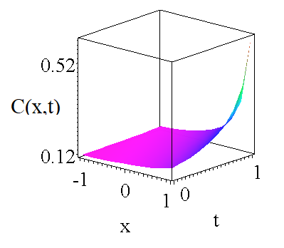
Figure 3: The concentration function $C(x,t)$ of Eq. (34) for the parameter set $c_{2}=0,\rho\cdot c_{p}=1,c=1,c_{1}=10,a=0.1$.

As a second class of functions we may consider a temporal and spatially periodic dependence of $\kappa(T[x,t])=b\sin(T[x,t])$ unfortunately we cannot derive any solution is a reasonable closed form. Additionally we tried the Lorenzian form of $\kappa(T[x,t])=\frac{a}{1+T(x,t)^{2}}$ and the exponential form of $\kappa(T[x,t])=b\cdot Exp(-T[x,t])$ in vain, there are no analytic closed form available.

3 Summary and Outlook

We investigated the highly non-linear diffusion equation where the diffusion constant (now it is rather a parameter) directly depends on the concentration. Two type of trial functions were used and different functional form were analyzed. We found physically relevant analytic solutions which have power law decays at infinite times. In the future - as a natural generalization - we try to investigate reactions diffusion equations which are diffusion equations with extra source terms on the right hand side.

4 Acknowledgment

- One of us (I.F. Barna) was supported by the NKFIH, the Hungarian National Research Development and Innovation Office.
- The authors declare no conflict of interest.
- Both authors contributed equally to every detail of the study.
- There was no extra external founding.
- All the evaluated data are available in the manuscript.

References

- [1] Ghez G., Diffusion Phenomena; Dover Publication Inc.: Long Island, NY, USA, 2001
- [2] Vogel G., Adventure Diffusion , Springer, 2019
- [3] Bird R.B., Stewart W.E. and Lightfoot E.N, Transport Phenomena, 2nd Edition, John Wiley & Sons, Inc., (2002)
- [4] Lienemann J., Yousefi A., Korvink J.V. Nonlinear Heat Transfer Modeling, In: Benner P. Sorensen D.C. Mehrmann V. (eds) Dimension Reduction of Large-Scale Systems, Lecture Notes in Computational Science and Engineering, 45, (2005) 327 https://link.springer.com/book/10.1007/3-540-27909-1
- [5] Thambynayagam R.K.M., The Diffusion Handbook: Applied Solutions for Engineers, McGraw-Hill: New York, 2011.
- [6] Bennett T.D., Transport by Advection and Diffusion John Wiley & Sons, Hoboken, NJ, 2013
- [7] Bluman G.W. and Cole J.D. , J. Math. Mech., 18, (1969) 1025
- [8] Reif F., Fundamentals of Statistical and Thermal Physics, Reissued by Waveland Press, Long Grove, 2009
- [9] Claus I., Gaspard P., Phys. Rev. E 63, (2001) 036227 https://doi.org/10.1103/PhysRevE.63.036227
- [10] Mátyás L., Gaspard P., Phys. Rev. E 71, (2005) 036147 https://doi.org/10.1103/PhysRevE.71.036147
- [11] Salma I., Füri P., Németh Z., Balásházy I., Hofmann W., Farkas Á, Atmospheric Environment 104, (2015) 39 https://doi.org/10.1016/j.atmosenv.2014.12.060
- [12] Mátyás L., Klages R., Physica D 187, (2004) 165 https://doi.org/10.1016/j.physd.2003.09.008
- [13] Mátyás L., Barna I.F., Chaos, Solitons & Fractals 44, (2011) 1111 http://dx.doi.org/10.1016/j.chaos.2015.08.002
- [14] Mátyás L. and Barna I.F. , Rom. J. Phys., 67, (2022) 101 https://rjp.nipne.ro/2022_67_1-2/RomJPhys.67.101.pdf
- [15] Barna I.F. and Mátyás L. Mathematics, 10, (2022) 3280 https://doi.org/10.3390/math10183281
- [16] Saleh M., Kovács E., Barna I.F. and Mátyás L. Mathematics 10, (2022) 2813 https://doi.org/10.3390/math10152813
- [17] Kovács E., Saleh M., Barna I.F. and Mátyás L. Diffusion Fundamentals 35, (2022) 70 https://diffusion.unileipzig.de/pdf/volume35/diff_fund_35(2022)70.pdf
- [18] Saleh M., Kovács E. and Barna I.F. Algorithms 16, (2023) 183 https://doi.org/10.3390/a16040184
- [19] Fujita, H. Textile Research Journal, 22, (1952) 823 https://doi.org/10.1177/004051755202201209
- [20] Pattle. R. E., Quart. Jouro. Mecb. and Applied Math., 12, (1959) 401 https://doi.org/10.1093/qjmam/12.4.407
- [21] Philip J. R., Australian Journal of Physics, 13, (1960) 1 https://api.semanticscholar.org/CorpusID:117850983
- [22] Boyer, R. H. Journal of Mathematics and Physics, 40, (1961) 41 https://doi.org/10.1002/sapm196140141
- [23] Bankoff, S. G., Advances in Chemical Engineering, 5, (1964) 75 https://doi.org/10.1016/s0065-2377(08)60007
- [24] Knight J. H. and J. R. Philip Journal of Engineering Mathematics, 8, (1974) 219 https://doi.org/10.1007/BF02353364
- [25] Tuck B, J. Phys. D: Appl. Phys. 9, (1976) 1559 https://doi.org/10.1088/0022-3727/9/11/005
- [26] Munier, A., Burgan, J. R., Gutierrez, J., Fijalkow, E., and Feix, M. R. SIAM Journal on Applied Mathematics, 40, (1981) 191 https://doi:10.1137/0140017
- [27] King J.R. J. Phys. A: Math. Gen. 24, (1991) 3213 https://doi.org/10.1088/0305-4470/24/14/010
- [28] Sadighi A. and Ganji D.D., Computers and Mathematics with Applications, 54, (2007) 1112 https://doi.org/10.1016/j.camwa.2006.12.077
- [29] Hayek M., Computers and Mathematics with Applications, 68, (2014) 1751 http://doi.org/10.1016/j.camwa.2014.10.015
- [30] Kosov A. A. and Semenov E. I., Siberian Mathematical Journal, 60, (2019) 93 https://doi.org/10.1134/S0037446619010117
- [31] Dorodnitsyn V. A. USSR Computational Mathematics and Mathematical Physics 22, (1982) 115. https://doi.org/10.1016/0041-5553(82)90102-1
- [32] Arrigo D.J., Hill J.M. and Broadbridge P., IMA Journal of Applied Mathematics, 52, (1994) 1 https://doi.org/10.1093/imamat/52.1.1
- [33] Vijayakumar K., J. Austral. Math. Soc. Set: B 39, (1998) 513 https://doi.org/10.1017/S0334270000007773
- [34] Cherniha R, and Serov M. Proceedings of the Second International Conference, Symmetry in Nonlinear Mathematical Physics Volume 2, (1997) 444 https://www.slac.stanford.edu/econf/C9707077/papers/symmetry1997.pdf
- [35] Chulián S., Rosa M. and Gandarias M. L. Journal of Computational and Applied Mathematics 354, (2019) 689 https://doi.org/10.1016/j.cam.2018.11.018
- [36] Liu H., Commun. Nonlinear Sci. Numer. Simulat. 36, (2016) 21 http://dx.doi.org/10.1016/j.cnsns.2015.11.019
- [37] Qu G.-Z. Wang G. and Wang M. Results in Physics, 23, (2021) 103971 https://doi.org/10.1016/j.rinp.2021.103971
- [38] Cattaneo, C. Atti del Seminario matematico e fisico della Università di Modenna, 3, (1948) 3
- [39] Cattaneo, C. Comptes Rendus de l’Académie des Sciences, 247, (1958) 431 https://gallica.bnf.fr/ark:/12148/bpt6k31993/f437.image.langEN
- [40] Vernotte, P. Comptes Rendus de l’Académie des Sciences, 246, (1965) 3154
- [41] Gurtin M.E. and Pipkin A.C., Archive for Rational Mechanics and Analysis volume 31, (1968) 113 https://link.springer.com/article/10.1007/BF00281373
- [42] Joseph, P. P. and Preziosi, L. Reviews of Modern Physics, 60, (1989) 41 https://journals.aps.org/rmp/abstract/10.1103/RevModPhys.61.41
- [43] Barna I.F. and Kersner R., J. Phys. A: Math. Theor. 43, (2010) 375210 http://iopscience.iop.org/1751-8121/43/37/375210
- [44] Kovács R. and Ván P. International Journal of Heat and Mass Transfer, 83, (2015) 613 https://doi.org/10.1016/j.ijheatmasstransfer.2014.12.045
- [45] Filipov S.M. and Faragó I. https://arxiv.org/abs/1811.06337
- [46] Muskat, M. The Flow of Homogeneous Fluids Through Porous Media. New York: McGraw-Hill. 1937
- [47] Barenblatt G.I. Prikladna ja Matematika i Mekhanika, 16, (1952) 67
- [48] Zeldovich, Y.B. and Raizer, Y.P. Physics of Shock Waves and High Temperature Hydrodynamic Phenomena (1st ed.). Academic Press 1966
- [49] Ames W.F., Nonlinear Partial Differential Equations in Engineering, vol. I,II, Academic Press, New York, 1965.
- [50] Fisher R.A., Annals of Eugenics 7, (1937) 353 https://doi.org/10.1111/j.1469-1809.1937.tb02153.x
- [51] Al-Khaled K., J. Comput. Appl. Math. 137, (2001) 245 https://core.ac.uk/download/pdf/82237548.pdf
- [52] Turing A., Philosophical Transactions of the Royal Society of London B. 237, (1952) 37 https://royalsocietypublishing.org/doi/pdf/10.1098/rstb.1952.0012
- [53] Arecchi F.T., Boccaletti S., Ramazza PL., Physics Reports 318, (1999) 1 https://doi.org/10.1016/S0370-1573(99)00007-1
- [54] Mazzoni T., A First Course in Quantitative Finance, Cambridge University Press, Cambridge, 2018
- [55] Lázár E., Acta Universitatis Sapientiae, Economics and Business 2, (2014) 75 https://intapi.sciendo.com/pdf/10.2478/auseb-2014-0011
- [56] Sedov L. Similarity and Dimensional Methods in Mechanics, CRC Press 1993.
- [57] Barna I.F. and Mátyás L. Chaos, Solitons and Fractals 78, (2015) 249 http://dx.doi.org/10.1016/j.chaos.2015.08.002
- [58] Barna I.F., Pocsai M.A. Lökös S. and Mátyás L. Chaos, Solitons and Fractals 103, (2017) 336 http://dx.doi.org/10.1016/j.chaos.2017.06.024
- [59] Barna I.F., Bognár G., Mátyás L. and Hriczó K., Journal of Thermal Analysis and Calorimetry 147, (2022) 13625 https://doi.org/10.1007/s10973-022-11574-3
- [60] Mátyás L. and Barna I.F., Universe 9, (2023) 264 https://doi.org/10.3390/universe9060264
- [61] Olver F.W.J., Lozier D.W., Boisvert R.F. and Clark C.W. NIST Handbook of Mathematical Functions, Cambridge University Press, 2010 https://dlmf.nist.gov/
- [62] Mező I., The Lambert W Function Its Generalizations and Applications, CRC Press, 2022
- [63] Hone J. et all. Appl. Phys. Lett. 77, (2000) 666 https://doi.org/10.1063/1.127079
- [64] Ezzahri Y., Ordonez-Miranda J. and Joulain K. Int. J. Heat Mass Transf 108, (2017) 1357 http://dx.doi.org/10.1016/j.ijheatmasstransfer.2017.01.024