Localization of scalar field on the brane-world by coupling with gravity

Abstract

In this paper, we consider a general coupling mechanism between the kinetic term and the background spacetime, in which a coupling function $F(R)$ is introduced into the kinetic term of the five-dimensional scalar field. Based on this scenario, we investigate the localization of scalar fields in three specific braneworld models: the Minkowski brane, the de Sitter brane, and the Anti-de Sitter brane. For each case, different types of the effective potentials can be achieved depending on the variation of the coupling parameter in the coupling function. The Minkowski brane can exhibit volcanic-like effective potential, Pöschl-Teller-like effective potential, or infinitely deep well. Both the de Sitter brane and Anti-de Sitter brane cases can realize Pöschl-Teller-like effective potential, or infinitely deep well. In addition, by setting the coupling parameters to specific values, the effective potentials of both the Minkowski brane and de Sitter brane cases can possess a positive maximum at the origin of the extra dimension. Lastly, in certain cases of the Anti-de Sitter brane, the Pöschl-Teller-like effective potentials allow for the existence of scalar resonances.

1 Introduction

The idea that our observed four-dimensional (4D) universe might be a 3-brane, embedded in a higher dimensional spacetime (the bulk), provides new insights for solving the gauge hierarchy and cosmological constant problems RubakovPLB1983 ; VisserPLB1985 ; AkamaLNP1983 ; Randall1999 ; LykkenJHEP2000 ; AntoniadisPLB1990 . Early theories involving extra dimensions, namely, the Kaluza$-$Klein (KK) type theories, were proposed to unify Einstein gravity and electromagnetism Appelquist . In braneworld scenarios, depending on the specific model, the size of the extra dimensions can vary. It has been suggested that the radii of the extra dimensions can be as large as a few Tev^-1 AntoniadisPLB1990 ; AntoniadisPRL2012 ; YangPRD2012 , or several millimeters AntoniadisPLB1998 , or even be infinitely large Randall1999 .

In the development of the braneworld theory, two types of brane models have been proposed: thin brane modes and thick brane models. The well-known thin brane models, namely the Arkani-Hamed-Dimopoulos-Dvali (ADD) brane model ArkaniPLB1998 ; AntoniadisPLB1998 and the Randall-Sundrum (RS) brane model Randall1999 , were primarily developed to address the hierarchy problem. However, the thickness of the brane was ignored in these theories, and thin brane was merely a mathematical idea. In the most fundamental theory, there seems to exist a minimum scale of length, thus the thickness of a brane should be considered in more realistic field models. For this reason, more natural thick brane models have been suggested De_Wolfe_PRD_2000 ; paper2002 ; Csaki_NPB_2000 ; Wang_PRD ; ThickBrane ; Bazeia ; 0910.0363 ; liu_0911.0269 ; Liu0907.1952 ; zhong_fRBrane ; Guo_BentBrane ; 1009.1684 ; SlatyerJHEP2007 .

In braneworld scenarios, the important issue is the localization of various bulk fields for the purpose of recovering the effective 4D gravity liu_0911.0269 ; Liu0907.1952 ; zhong_fRBrane ; LiuPRD1101.4145 ; ZhongEPJC2016 ; Zhong1711.09413 and building up the Standard Model German1210.0721 ; LiuZJHEP2008 ; liu_0911.0269 ; JonesMPRD2013 ; Pomarol9911294 ; BajcPLB2000 ; OdaPLB2000 ; SousaSPLB2013 ; RubinEPJC2015 ; GherghettaPNPB2000 ; YoumNPB2000 ; AbeKPRD2003 ; GhorokuY2003 ; OdaPLB2003 ; Ghoroku0106145 ; Liu0708.0065 ; Jardim1411.6962 ; Zhao1712.09843 . In a braneworld model, except for the localized zero modes of various fields, there are massive KK modes of these fields which can move freely along the extra dimension, be localized, or be quasi-localized on the brane LiuPRD0904 . These quasi-localized modes are referred to as resonance KK modes. Extensive research has been conducted on the resonances of various fields in the context of extra-dimensional theories Almeida2009 ; CruzPLB2014 ; XuEPJC2015 ; CsakiPRL2000 ; ZhangDuPRD2016 ; ZhongZEPJC2018 ; GuoZPLB2020 ; SuiGPRD2020 ; TanGEPJC2021 ; ChenGEPJC2021 ; TanEPJC2023 , as well as on the study of these massive dynamic resonances around black holes BarrancoPRD2012 ; BarrancoPRL2012 ; BarrancoPRD2014 ; Zhou1308.2863 ; Gossel1308.6426 ; Sampaio1406.3536 ; Degollado1408.2589 ; Sanchis1412.8304 ; Haung1708.0476 ; Sporea1905.05086 . Among these investigations, the localization of scalar fields plays a vital role. It is critical not only for phenomenological model-building but also for the dynamic description of the models. Scalar particles or scalar fields, such as the Higgs boson HiggsPL1964 ; HiggsPRL1964 ; ATLAS1207.7214 , the only elementary particle in the Standard Model, scalar perturbations within the framework of gravity localization in braneworld theories liu_0911.0269 ; LiuPRD1101.4145 ; ZhongEPJC2016 ; Zhong1711.09413 , and scalar fields derived from the duality relation in 4D spacetime Mukhopadhyaya ; Quevedo1011.1491 , constitute essential and highly desirable subjects. For the reasons stated above, the investigation into the localization of scalar fields holds fundamental importance within the realm of physics.

Regarding the localization of the scalar field, a focus point of our discussion, the scalar zero mode can be localized on brane of different types BajcPLB2000 . Specifically, in the case of the Minkowski (M₄) brane, the effective potential in corresponding Schrödinger-like equation takes the forms of a series of volcanic-like effective potentials LiuZJHEP2008 ; LiangPLB2009 ; Guo1912.01396 , and the scalar zero mode can be localized on the brane while the massive scalar KK modes cannot. In Refs. OdaPLB2000 ; AntoninoPRD2009 , the authors realized the localization of the scalar zero mode in the six-dimensional braneworld models. Moreover, Ref. LiuZJHEP2008 showed that under a specific condition, there will be an additional localized massive mode on the Weyl thick brane. In the case of the de Sitter (dS₄) brane, the effective potentials belong to the Pöschl-Teller-like effective potentials LiangDPLB2009 ; LiuJCAP20090203 ; GuoPRD201305 . These potentials lead to the localization of scalar zero modes on the brane as well as mass gaps in the mass spectra. In the case of the Anti-de Sitter (AdS₄) brane, there exist infinitely deep potential wells LiuJHEP201002 ; LiuPRD1101.4145 , capable of trapping an infinite number of massive scalar modes. However, localizing the scalar zero mode on the AdS₄ brane requires the fine-tuning of parameters after introducing a coupling potential LiuJHEP201002 .

In this paper, we consider three coupling mechanisms: the general coupling between the kinetic term and the spacetime, the coupling between the five-dimensional (5D) scalar field and the spacetime, and the coupling between the 5D scalar field and the background scalar field which generates the brane. The introducing of the latter two coupling mechanisms leads to the localization of scalar zero mode on the AdS₄ brane. Then, we focus on the first one. Based on this scenario, we explore the localization of the scalar field with braneworld models characterized by three different types of brane geometries: Minkowski, dS₄, and AdS₄. In the case of the Minkowski brane, we observe the emergence of volcanic-like effective potential, Pöschl-Teller-like effective potential, and an infinitely deep well. These potentials are determined by coupling parameter present in the coupling function $F(R)$. The scalar zero mode can be localized on the brane when the coupling parameter is real. Besides, in certain instances with a negative coupling parameter, the effective potential will exhibit a positive maximum at the origin of the extra dimension. Similarly, in the dS₄ brane case, we can realize Pöschl-Teller-like effective potential and infinitely deep well. The scalar zero mode can be localized with a real coupling parameter. Furthermore, under specific negative values of the coupling parameter, an effective potential with a positive maximum at the origin of the extra dimension, similar to that of the Minkowski brane case, can exist. Lastly, in the AdS₄ brane case, there could be Pöschl-Teller-like effective potential or infinitely deep well. For a coupling parameter $t>2.5$, the zero mode can be localized on the brane, whereas for $t=2.5$, the localization depends on the specific values of parameters of the model. Moreover, in the latter case, introducing another parameter into the function $F(R)$ could lead to presence of the Pöschl-Teller-like effective potentials which allow for the existence of scalar resonances.

The organization of this paper is as follows: We provide a review of our method in Sec. 2. The localization of the scalar zero mode and massive modes is discussed in Sec. 2.1 and Sec 2.2, respectively. Applying our method to the concrete braneworld models are shown in the next section, in which we discuss the case of Minkowski brane in Sec. 3.1, dS₄ brane in Sec. 3.2 and AdS₄ brane in Sec. 3.3. The conclusion is given in Sec. 4.

2 The Method

We start with the 5D line element (the $[-,+,+,+,+]$ signature will be assumed below)

$$\mathrm{d}s^{2}={g}_{MN}\mathrm{d}x^{M}dx^{N}=e^{2A(y)}\hat{g}_{\mu\nu}\mathrm{d}x^{\mu}\mathrm{d}x^{\nu}+\mathrm{d}y^{2},$$ (1)

where $\text{e}^{2A(y)}$ is the warp factor, $\hat{g}_{\mu\nu}$ is the induced metric of the 3-brane, and $y=x^{5}$ denotes the extra dimension. Throughout this paper, capital Latin letters $M,N,...=0,1,2,3,5$ and Greek letters $\mu,\nu,...=0,1,2,3$ are used to represent the bulk and brane indices, respectively.

With the above metric (1), the scalar curvature $R$ of the bulk can be expressed as

$$R(y)=4\text{e}^{-2A(y)}\Lambda-8\partial_{y,y}A(y)-20(\partial_{y}A(y))^{2},$$ (2)

where $\Lambda$ is some constant such that $\hat{R}=4\Lambda$. In the case of an AdS₄ brane cosmology, $\Lambda$ is negative, while for a dS₄ brane cosmology, it is positive. And a Minkowski spacetime corresponds to the case $\Lambda=0$. The braneworld which holds an five-dimensional (asymptotic) de Sitter (dS₅) spacetime or (asymptotic) Anti-de Sitter (AdS₅) spacetime at infinity suggests that the scalar curvature $R$ satisfies

$$R(y\rightarrow\infty)\rightarrow\left\{\begin{array}[]{llcll}{\mathrm{C}_{R}}_{1}&&\mathrm{dS_{5}~{}spacetime}\\ -{\mathrm{C}_{R}}_{2}&&\mathrm{AdS_{5}~{}spacetime},\end{array}\right.$$ (3)

where ${\mathrm{C}_{R}}_{1}$ and ${\mathrm{C}_{R}}_{2}$ are positive constants.

We assume the 5D action for a real scalar field $\Phi$ as

$$S=\int d^{5}x\sqrt{-g}~{}\bigg{[}-\frac{1}{2}F(R)g^{MN}\partial_{M}\Phi\partial_{N}\Phi-\xi R\Phi^{2}-V(\Phi,\phi)\bigg{]},$$ (4)

where the factor $F(R)$ is the coupling function representing the general coupling between the kinetic term and the spacetime. We suggest that $F(R)$ is a function dependent on the scalar curvature of the bulk. The term $\xi R\Phi^{2}$ describes the coupling between the 5D scalar field $\Phi$ and the spacetime, with $\xi$ as the coupling parameter. The potential $V(\Phi,\phi)$ is a coupling potential of 5D scalar field $\Phi$ to itself and to the background scalar field $\phi$ which generates the brane. Besides, the potential $V(\Phi,\phi)$ should include terms $\Phi,\Phi^{2},\Phi^{3},\Phi^{4}$ and $(\phi\Phi)^{2}$, among which the terms $\Phi$ and $\Phi^{3}$ can be eliminated by considering a discrete symmetry. Thus, we can set DaviesPRD07

$$V(\Phi,\phi)=(\lambda\phi^{2}-u^{2})\Phi^{2}+\tau\Phi^{4},$$ (5)

where $\lambda,u$ and $\tau$ are parameters. To start with, we discuss briefly the effects of the potential $V(\Phi,\phi)$ and the coupling term $\xi R\Phi^{2}$. For simplicity, we set function $F(R)=1$. Then, the localization of the scalars will be studied with the assistance of the mass-independent potential of scalar KK modes in the corresponding Schrödinger equation. In order to obtain this potential, we perform the coordinate transformation

$$dz=\text{e}^{-A(y)}dy,$$ (6)

where the coordinate $z$ is a conformal coordinate of $y$. Next, based on the action (4), we carry out the similar calculations to that shown in Ref. LiuJHEP201002 . The mass-independent potential can be expressed as

$$V(z)=\frac{3}{2}\partial_{z,z}A(z)+\frac{9}{4}(\partial_{z}A(z))^{2}+2e^{2A(z)}(\xi R+\lambda\phi^{2}-u^{2}).$$ (7)

Meanwhile, the scalar curvature $R$ in terms of coordinate $z$ can be obtained:

$$R(z)=4\text{e}^{-2A(z)}\left(\Lambda-2\partial_{z,z}A(z)-3(\partial_{z}A(z))^{2}\right).$$ (8)

And then, the potential (7) is recast to

$$V(z)=(\frac{3}{2}-16\xi)\partial_{z,z}A(z)+(\frac{9}{4}-24\xi)(\partial_{z}A(z))^{2}+2e^{2A(z)}(\lambda\phi^{2}-u^{2})+8\xi\Lambda.$$ (9)

Compared to the effective potential presented in Ref. LiuJHEP201002 , the effective potential $V(z)$ (9) contains similar terms, but the coefficients of these terms have been modified due to the presence of the coupling term $\xi R\Phi^{2}$. Thus, referring to the results in Ref. LiuJHEP201002 , we can draw the conclusion that by introducing the potential $V(\Phi,\phi)$ and the term $\xi R\Phi^{2}$, the limits of the effective potential $V(z)$ can be altered when far away from the brane, while the types of potential remain unchanged. Consequently, additional massive scalar modes can be localized on the Minkowski or dS₄ brane, or the scalar zero mode can be localized on the AdS₄ brane through the fine-tuning of parameters, which holds significant implications.

Then, we turn attention to the general coupling mechanism between the kinetic term and the spacetime. In order to describe its effects distinctly, we consider neither the potential $V(\Phi,\phi)$ nor the coupling terms $\xi R\Phi^{2}$ with the parameters $\lambda=0,u=0$, and $\xi=0$ below. Hence, the 5D action (4) turns into the following one:

$$S=-\frac{1}{2}\int d^{5}x\sqrt{-g}~{}F(R)g^{MN}\partial_{M}\Phi\partial_{N}\Phi.$$ (10)

The rules that confirm the form of function $F(R)$ are:

1. In the case where the scalar curvature $R\to 0$, the bulk spacetime becomes flat, and the general coupling vanishes. Then, the action (10) returns to the standard form:

   $$S=-\frac{1}{2}\int d^{5}x\sqrt{-g}~{}g^{MN}\partial_{M}\Phi\partial_{N}\Phi.$$ (11)

2. The function $F(R)$ should satisfy the positivity condition

   $$F(R)>0$$ (12)

   to preserve the canonical form of 4D action.

Note that the restriction mentioned in the second item is less strict in comparison to the one described in Ref. Zhao1712.09843 . This is because the metric $g_{MN}$ and the 5D scalar $\Phi$ incorporate extra-dimensional components.

2.1 Localization of the Zero Mode

In order not to contradict with the present observations, the zero mode of the scalar field should be confined on the brane, which will impose some constraints on the function $F(R)$. We have implicitly assumed that bulk scalar fields considered in this paper make little contribution to the bulk energy, so that the solutions given below remain valid even in the presence of bulk scalar fields.

Let us introduce the decomposition

$$\Phi(x^{\mu},y)=\sum_{n}\phi_{n}(x^{\mu})\chi_{n}(y),$$ (13)

where $\phi_{n}(x^{\mu})$ are the 4D scalar fields, and the scalar KK modes $\chi_{n}(y)$ are supposed to be functions of the coordinate $y$. Then, the 5D action (10) can be reduced to

$$S=-\frac{1}{2}\int\mathrm{d}yF(R)e^{2A}\chi_{n}^{2}(y)\int\mathrm{d}^{4}x\sqrt{-\hat{g}}\left(\hat{g}^{\mu\nu}\partial_{\mu}\phi_{n}\partial_{\nu}\phi_{n}+m_{n}^{2}\phi_{n}^{2}\right),$$ (14)

where $\chi_{n}(y)$ satisfy the following equation

$$\chi_{n}^{\prime\prime}+\left(4A^{\prime}+\frac{F^{\prime}(R)}{F(R)}\right)\chi_{n}^{\prime}=-m_{n}^{2}\chi_{n}e^{-2A},$$ (15)

with the boundary conditions either the Neumann $\chi_{n}^{\prime}(\pm\infty)=0$ or the Dirichlet $\chi_{n}(\pm\infty)=0$, where the prime stands for the derivative with respect to $y$ in this subsection.

The localization of the scalar field requires

$$\int_{-\infty}^{+\infty}\mathrm{d}yF(R)e^{2A}\chi_{n}^{2}(y)=1.$$ (16)

For the zero mode, $m_{0}=0$, so Eq. (15) reads

$$\chi_{0}^{\prime\prime}+\left(4A^{\prime}+\frac{F^{\prime}(R)}{F(R)}\right)\chi_{0}^{\prime}=0.$$ (17)

By setting $\gamma^{\prime}=4A^{\prime}+\frac{F^{\prime}(R)}{F(R)}$, the above equation (17) becomes

$$\chi_{0}^{\prime\prime}+\gamma^{\prime}\chi_{0}^{\prime}=0,$$ (18)

from which the general solution of zero mode is

$$\chi_{0}=\mathrm{c}_{0}+\mathrm{c}_{1}\int e^{-\gamma}\mathrm{d}y.$$ (19)

Here $\mathrm{c}_{0}$ and $\mathrm{c}_{1}$ are arbitrary integration constants. The braneworld discussed here holds $\mathbb{Z}_{2}$ symmetry along the extra dimension. The functions $F(R),A(y)$ and $\gamma$ are all even functions of the coordinate $y$, which makes the second term in Eq. (19) is odd. When imposing the Dirichlet boundary condition $\chi_{n}(\pm\infty)=0$, it leads to $\mathrm{c}_{0}=0$ and $\mathrm{c}_{1}=0$. On the other hand, the Neumann boundary condition $\chi^{\prime}_{n}(\pm\infty)=0$ only lead to $\mathrm{c}_{1}=0$. Consequently, the zero mode solution is

$$\chi_{0}=\mathrm{c}_{0}.$$ (20)

The localization of zero mode requires the following condition

$$\int_{-\infty}^{+\infty}\mathrm{d}yF(R)e^{2A}\chi_{0}^{2}(y)$$ (21)

$$= \mathrm{c}_{0}^{2}\int_{-\infty}^{+\infty}\mathrm{d}yF(R)e^{2A}=1.$$

Therefore, whether the above integration (21) converges is determined by the asymptotic behaviors of both the function $F(R)$ and the warp factor $e^{2A}$ when far away from the brane. Specifically, the convergent condition is

$$F(R(y\to\pm\infty))\propto y^{-p}e^{-2A}$$ (22)

with $p>1$. From this expression, we know that the localization of scalar zero mode are model$-$dependant. The further discussions will be presented explicitly based on specific braneworld models in Sec. 3.

2.2 Localization of Massive Modes

The localization of massive modes is determined by the shapes of the effective potentials for scalar KK modes in the corresponding Schrödinger-like equation.

According to the action (10), by employing the KK decomposition

$$\Phi(x^{\mu},y)=\sum_{n}\phi_{n}(x^{\mu})\tilde{\chi}_{n}(y)e^{-2A(y)}(F(R))^{-\frac{1}{2}}$$ (23)

and demanding $\phi_{n}(x^{\mu})$ satisfy the 4D massive Klein$-$Gordon equation

$$\bigg{(}\frac{1}{\sqrt{-\hat{g}}}\partial_{\mu}(\sqrt{-\hat{g}}\hat{g}^{\mu\nu}\partial_{\nu})-m_{n}^{2}\bigg{)}\phi_{n}=0,$$ (24)

we can obtain the equation for the scalar KK modes $\tilde{\chi}_{n}(y)$ as

$$\left[-\partial^{2}_{y}+V(y)\right]{\tilde{\chi}}_{n}(y)=m_{n}^{2}{\tilde{\chi}}_{n}(y)e^{-2A(y)},$$ (25)

in which

$$V(y)=2A^{\prime\prime}(y)+4A^{\prime 2}(y)+\frac{F^{\prime\prime}(R)}{2F(R)}+\frac{2A^{\prime}(y)F^{\prime}(R)}{F(R)}-\frac{F^{\prime 2}(R)}{4F^{2}(R)}.$$ (26)

Here the scalar KK modes $\tilde{\chi}_{n}(y)=\chi_{n}(y)e^{2A(y)}(F(R))^{\frac{1}{2}}$, $m_{n}$ is the mass of the scalar KK excitations and the prime denotes derivative with respect to $y$.

Furthermore, Eq. (25) can be factorized into the following one

$$\bigg{(}\frac{\mathrm{d}}{\mathrm{d}y}+\Gamma^{\prime}(y)\bigg{)}\bigg{(}-\frac{\mathrm{d}}{\mathrm{d}y}+\Gamma^{\prime}(y)\bigg{)}\tilde{\chi}_{n}(y)=m_{n}^{2}\tilde{\chi}_{n}(y)e^{-2A(y)},$$ (27)

where there is

$$\Gamma^{\prime}(y)=2A^{\prime}(y)+\frac{F^{\prime}(R)}{2F(R)}.$$ (28)

Without loss of the generality, we can take

$$\Gamma(y)=2A(y)+\frac{1}{2}\ln{F(R)}.$$ (29)

Then, the solution of the scalar zero mode can be obtained from Eq. (27) as

$$\tilde{\chi}_{0}(y)=N_{1}e^{2A(y)}(F(R))^{\frac{1}{2}},$$ (30)

where $N_{1}$ is the normalization constant. The localization of scalar zero mode $\tilde{\chi}_{0}(y)$ requires

$$\int\mathrm{d}y\tilde{\chi}^{2}_{0}(y)=N_{1}^{2}\int\mathrm{d}yF(R)e^{4A(y)}=1.$$ (31)

On the other hand, it can be observed that the potential $V(y)$ in Eq. (25) represents the effective potential for the scalar zero mode, rather than for the massive ones. To address this issue, we will proceed with our discussions in terms of the conformal coordinate $z$, instead of the coordinate $y$. By performing the coordinate transformation (6), the metric (1) can be expressed as

$$\mathrm{d}s^{2}=e^{2A(z)}(\hat{g}_{\mu\nu}\mathrm{d}x^{\mu}\mathrm{d}x^{\nu}+\mathrm{d}z^{2}).$$ (32)

And we can obtain the equation of motion derived from the action (10) as

$$\frac{1}{\sqrt{-\hat{g}}}\partial_{\mu}(\sqrt{-\hat{g}}\hat{g}^{\mu\nu}\partial_{\nu}\Phi)+\frac{e^{-3A(z)}}{F(R)}\partial_{z}(e^{3A(z)}\partial_{z}\Phi)=0.$$ (33)

Through the KK decomposition

$$\Phi(x^{\mu},z)=\sum_{n}\phi_{n}(x^{\mu}){\tilde{\chi}}_{n}(z)e^{-\frac{3}{2}A(z)}(F(R))^{-\frac{1}{2}},$$ (34)

and demanding $\phi_{n}(x^{\mu})$ satisfies the 4D Klein-Gordon equation (24), we can further obtain the equation for scalar KK modes $\tilde{\chi}_{n}(z)$:

$$\left[-\partial^{2}_{z}+V(z)\right]{\tilde{\chi}}_{n}(z)=m_{n}^{2}{\tilde{\chi}}_{n}(z),$$ (35)

which is a Schrödinger-like equation with the effective potential given by

$$V(z)=\frac{3}{2}A^{\prime\prime}(z)+\frac{9}{4}A^{\prime 2}(z)+\frac{F^{\prime\prime}(R)}{2F(R)}+\frac{3A^{\prime}(z)F^{\prime}(R)}{2F(R)}-\frac{F^{\prime 2}(R)}{4F^{2}(R)},$$ (36)

where the prime denotes the derivative with respect to $z$ here. This effective potential $V(z)$ is just the mass-independent potential.

Similarly, the Schrödinger-like equation (35) can be recast to

$$\bigg{(}\frac{\mathrm{d}}{\mathrm{d}z}+\Gamma^{\prime}(z)\bigg{)}\bigg{(}-\frac{\mathrm{d}}{\mathrm{d}z}+\Gamma^{\prime}(z)\bigg{)}\tilde{\chi}_{n}(z)=m_{n}^{2}\tilde{\chi}_{n}(z),$$ (37)

where there is

$$\Gamma^{\prime}(z)=\frac{3}{2}A^{\prime}(z)+\frac{F^{\prime}(R)}{2F(R)}.$$ (38)

From the above expression (37), we can see that there are no normalizable modes with negative $m_{n}^{2}$, namely, there is no tachyonic scalar mode. Thus, the scalar zero mode is the lowest mode in the spectrum.

From Eq. (38), without loss of the generality, we can take

$$\Gamma(z)=\frac{3}{2}A(z)+\frac{1}{2}\ln{F(R)}.$$ (39)

And based on Eq. (37), the solution of the scalar zero mode is easy to be found:

$$\tilde{\chi}_{0}(z)=N_{2}e^{\frac{3}{2}A(z)}(F(R))^{\frac{1}{2}},$$ (40)

with $N_{2}$ the normalization constant. This zero mode solution can be related to the one expressed in terms of the coordinate $y$ (30) through the decomposition (23) and (34).

Returning to the discussion of the massive modes, the action of the 5D scalar field (10) can be reduced to

$$S=-\frac{1}{2}\int\mathrm{d}z\tilde{\chi}_{n}^{2}(z)\int\mathrm{d}^{4}x\sqrt{-\hat{g}}\left(\hat{g}^{\mu\nu}\partial_{\mu}\phi_{n}\partial_{\nu}\phi_{n}+m_{n}^{2}\phi_{n}^{2}\right),$$ (41)

in which the Schrödinger-like equation (35) should be satisfied. In order to get the effective action for the 4D scalar field, the orthonormality condition needs to be introduced:

$$\int\mathrm{d}z\tilde{\chi}_{m}(z)\tilde{\chi}_{n}(z)=0.~{}~{}~{}(m\neq n)$$ (42)

And this equation contains the localization condition for $\tilde{\chi}_{n}(z)$

$$\int\mathrm{d}z\tilde{\chi}^{2}_{n}(z)<\infty.$$ (43)

The existence of localized massive scalar KK modes is determined by the shapes of the effective potential $V(z)$ (36), which is influenced by both the functions $F(R(z))$ and $A(z)$. With specific braneworld models and the corresponding functions $F(R)$, the localization of massive scalar KK modes will be discussed below.

3 Concrete Braneworld Models

In this section, we will describe the localization of the scalar field while considering the general coupling between the kinetic term and the spacetime. These processes will be presented using specific braneworld models that incorporate three different cases of brane geometries: Minkowski, dS₄ and AdS₄, respectively.

3.1 Minkowski Brane

In the case of the constant $\Lambda=0$, the brane is flat (Minkowski brane) and the 5D line element (1) turns into

$$\mathrm{d}s^{2}=e^{2A(y)}\hat{\eta}_{\mu\nu}\mathrm{d}x^{\mu}\mathrm{d}x^{\nu}+\mathrm{d}y^{2},$$ (44)

where $\hat{\eta}_{\mu\nu}$ denotes the metric of the Minkowski brane. And the scalar curvature (2) becomes

$$R(y)=-8A^{\prime\prime}(y)-20A^{\prime 2}(y).$$ (45)

Here, we consider a trial warp factor of Minkowski brane and it takes the form SlatyerJHEP2007

$$A(y)=-a^{2}\left(\frac{2}{3}\ln(\cosh(by))-\frac{1}{6}(\textrm{sech}(by))^{2}+c\right),$$ (46)

where $a,b$ and $c$ are constants, among which $a$ is dimensionless, $b$ has dimensions of inverse length, and $c$ is a dimensionless integration constant. This warp factor has even-parity with respect to $y$, and the braneworld model exhibits $\mathbb{Z}_{2}$ symmetry. As a result, we will solely concentrate on the asymptotic behaviors of the model as $y\rightarrow+\infty$ in the following discussion.

With this warp factor (46), the scalar curvature (45) has solution:

$$R(y)=\frac{4}{9}a^{2}b^{2}\bigg{(}18(\textrm{sech}(by))^{4}-5a^{2}\left(2+(\textrm{sech}(by))^{2}\right)^{2}(\tanh(by))^{2}\bigg{)}.$$ (47)

And then, its asymptotic solution as $y\rightarrow\infty$ is

$$R(y\rightarrow\infty)\rightarrow-l+me^{-4by},$$ (48)

where parameters $l=\frac{80}{9}a^{4}b^{2},m=\frac{64(15a^{2}+18)}{9}a^{2}b^{2}$, for simplicity.

Meanwhile, the asymptotic expression of $e^{A(y)}$ as $y\rightarrow\infty$ can be given by

$$e^{2A(y)}\rightarrow pe^{-qy},$$ (49)

where $p=e^{-\frac{a^{2}}{3}(6c-4\ln{2})}$ and $q=\frac{4}{3}a^{2}b$.

In this case of a Minkowski brane, we suggest the function $F(R)$ takes the form of

$$F(R)=e^{(\mathrm{C}_{1})^{t}-(\frac{\mathrm{C}_{1}l}{R+l})^{t}},$$ (50)

where $t$ is the coupling parameter, and $\mathrm{C}_{1}$ is an arbitrary positive constant that is chosen to satisfy the condition $F(R=0)=1$. From this expression, we can obtain the asymptotic solution of $F(R)$ as $y\rightarrow\infty$:

$$F(R)\rightarrow we^{-ne^{4bty}},$$ (51)

where parameters $w=e^{(\mathrm{C}_{1})^{t}}$ and $n=(\frac{\mathrm{C}_{1}l}{m})^{t}$, for simplicity.

Returning to the discussion of the scalar zero mode (30), along with Eq. (49) and Eq. (51), the asymptotic solution for the scalar zero mode $\tilde{\chi}_{0}(y\rightarrow\infty)$ can be given by

$$\tilde{\chi}_{0}(y\rightarrow\infty)\rightarrow N_{1}pw^{\frac{1}{2}}e^{-qy}e^{-\frac{1}{2}(\frac{\mathrm{C}_{1}l}{m})^{t}e^{4bty}}.$$ (52)

The localization of the zero mode requires

$$\int\mathrm{d}y\tilde{\chi}_{0}^{2}(y)<\infty.$$ (53)

From Eq. (52), there is

$$\tilde{\chi}_{0}^{2}(y\rightarrow\infty)\rightarrow N_{1}^{2}p^{2}we^{-2qy}e^{-(\frac{\mathrm{C}_{1}l}{m})^{t}e^{4bty}}.$$ (54)

It is evident that this condition is satisfied with an arbitrary real constant $t$. And the scalar zero mode $\tilde{\chi}_{0}(y)$ will be normalizable. We plot the zero mode in terms of both the coordinate $y$ and the coordinate $z$ in Fig. 1. The parameters used for the plot are $\mathrm{C}_{1}=2,a=1,b=2,c=1$, and the coupling parameter $t$ is set to $\frac{a^{2}}{10},\frac{a^{2}}{6}$ and $\frac{a^{2}}{4}$, respectively.

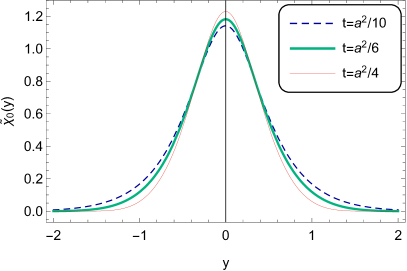
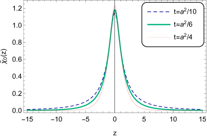
Figure 1: Plots of the zero mode in terms of the coordinate $y$ ($\tilde{\chi}_{0}(y)$ for left figure) and the coordinate $z$ ($\tilde{\chi}_{0}(z)$ for right figure) with parameters $\mathrm{C}_{1}=2,a=1,b=2$ and $c=1$. The coupling parameter is set as $t=\frac{a^{2}}{10}$ for the dashed line, $t=\frac{a^{2}}{6}$ for the thick line and $t=\frac{a^{2}}{4}$ for the thin line, respectively.

However, in the context of the braneworld model considered here, obtaining an analytic solution for the warp factor with respect to $z$, as well as for the effective potential $V(z)$ (36), is challenging. Consequently, we will employ numerical methods to calculate the solution for the potential $V(z)$.

Carrying out the coordinate transformation (6), we can express the effective potential $V(z)$ in terms of $z$ as follows

$$V(z(y))= \frac{15}{4}e^{2A(y)}A^{\prime 2}(y)+\frac{3}{2}e^{2A(y)}A^{\prime\prime}(y)$$ (55)

$$+\frac{e^{2A(y)}F^{\prime\prime}(R)}{2F(R)}+\frac{2e^{2A(y)}A^{\prime}(y)F^{\prime}(R)}{F(R)}$$

$$-\frac{e^{2A(y)}F^{\prime 2}(R)}{4F^{2}(R)}.$$

Next, by substituting the asymptotic solutions of the warp factor (48) and the function $F(R)$ (51) into the potential $V(z(y))$ (55), we can get its asymptotic solution as $y\rightarrow\infty$:

$$V(z(y\rightarrow\infty))\rightarrow\mathrm{C}_{2}t^{2}e^{(8bt-q)y}+(\mathrm{C}_{3}t-\mathrm{C}_{4}t^{2})e^{(4bt-q)y},$$ (56)

where $\mathrm{C}_{2}$, $\mathrm{C}_{3}$ and $\mathrm{C}_{4}$ are positive constants. From this expression, it can be concluded that the effective potential has the following asymptotic behaviors:

$$V(z(y\rightarrow\infty))\rightarrow\left\{\begin{array}[]{llcll}+\infty&&t&>\frac{a^{2}}{6}\\ \mathrm{C}&&t&=\frac{a^{2}}{6}\\ 0&&t&<\frac{a^{2}}{6},\end{array}\right.$$ (57)

with $\mathrm{C}$ a positive constant.

The shapes of both the effective potential $V(z(y))$ and the numerical solution of the effective potential $V(z)$ are depicted in Fig. 2. The parameters used are $\mathrm{C}_{1}=2,a=1,b=2,c=1$, and coupling parameter $t$ is set to $\frac{a^{2}}{10},\frac{a^{2}}{6}$ and $\frac{a^{2}}{4}$, respectively. We can observe that the shapes of the two expressions for the effective potential are similar. However, the one expressed in terms of the coordinate $z$ is extends along the extra dimension in comparison to the other. The figures depict a volcano-like effective potential when the coupling parameter $t=\frac{a^{2}}{10}$. This suggests the presence of a continuous gapless spectrum of scalar KK modes with no mass gap separating them from the zero mode. Additionally, two potential barriers symmetrically appear neighbouring the brane. In the case of $t=\frac{a^{2}}{6}$, there will be a P$\ddot{\mathrm{o}}$schl-Teller-like effective potential. This configuration introduces a mass gap that separates the zero mode from the continuous spectrum of massive KK modes. Finally, when the parameter $t$ is set to $\frac{a^{2}}{4}$, the effective potential $V(z)$ exhibits an infinitely deep well, supporting infinite bound KK modes. We show a few lower localized massive solutions with numerical methods in Fig. 3. As the pictures demonstrate, all the massive scalar KK modes are localized on the brane, giving rise to an infinite discrete spectrum of mass.

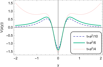
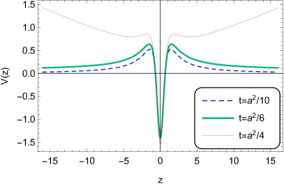
Figure 2: Plots of the effective potential $V(z(y))$ and the numerical solution of effective potential $V(z)$ with parameters $\mathrm{C}_{1}=2,a=1,b=2$ and $c=1$. The coupling parameter is set as $t=\frac{a^{2}}{10}$ for the dashed line, $t=\frac{a^{2}}{6}$ for the thick line, and $t=\frac{a^{2}}{4}$ for the thin line, respectively.

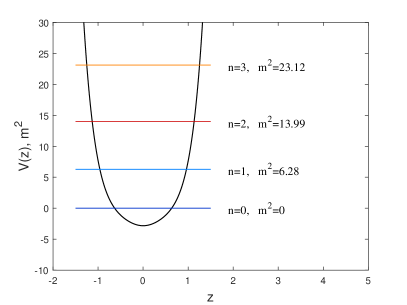
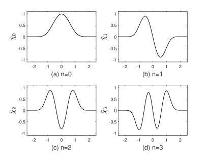
Figure 3: In the left figure, the black line represents the effective potential $V(z)$, and the colored lines depict the positions of mass spectra. The right figure displays the corresponding solutions of $\tilde{\chi}_{n}(z)$. The parameters are set as $\mathrm{C}_{1}=2,a=1,b=2,c=1$ and $t=1$.

On the other hand, the effective potential $V(z(y))$ at $y=0$ is

$$V(z(y=0))=\frac{3b^{2}e^{\frac{1}{3}a^{2}(1-6c)}(-a^{2}(9+10a^{2})-3(4+5a^{2})(\frac{10a^{2}\mathrm{C}_{1}}{9+10a^{2}})^{t}t)}{18+20a^{2}}.$$ (58)

Setting $V(z(y=0))=0$, we can get

$$case~{}\text{I}: t=\frac{-9a^{2}-10a^{4}}{3(4+5a^{2})},\ \ \ \ \ \mathrm{C}_{1}=\frac{9+10a^{2}}{10a^{2}};$$ (59)

$$case~{}\text{II}: t=\frac{\mathrm{ProductLog}\bigg{[}\mathrm{C}_{5},-\frac{(9a^{2}+10a^{4})(\ln(\frac{10a^{2}\mathrm{C}_{1}}{9+10a^{2}}))}{3(4+5a^{2})}\bigg{]}}{\ln(\frac{10a^{2}\mathrm{C}_{1}}{9+10a^{2}})},$$ (60)

$$\mathrm{C}_{1}\neq\frac{9+10a^{2}}{10a^{2}}\text{ and }\mathrm{C}_{5}\in Integers,$$

where ProductLog is the Lambert $W-$function.

For $case~{}\text{I}$, by setting $\mathrm{C}_{1}=\frac{9+10a^{2}}{10a^{2}}$, $V(z(y=0))$ can be expressed as

$$V(z(y=0))=-\frac{3b^{2}e^{\frac{1}{3}a^{2}(1-6c)}(10a^{4}+12t+3a^{2}(3+5t))}{18+20a^{2}},$$ (61)

which is a linear expression with respect to $t$. The effective potential for various values of $t$ is depicted in Fig. 4(a). From this figure, we can see that the effective potential at $y=0$ decreases monotonously as $t$ increases.

For $case~{}\text{II}$, we present the shapes of $V(z(y=0))$ concerning the parameter $t$ in Fig. 4(b) with parameters $a=1,b=2,c=1$, and $\mathrm{C}_{1}=2$. Note that we only consider real values of $t$ as defined in Eq. (60), which are given by:

$$\{-95.79420,-0.73057\}.$$ (62)

These two values correspond to $\mathrm{C}_{5}=-1$ and $0$, respectively. From Fig. 4(b), we observe that the potential $V(z(y))$ at $y=0$ is positive within the range of $(-95.79420,-0.73057)$.

Given the scalar zero mode is normalizable, a positive potential $V(z(y))$ at $y=0$ implies the existence of negative wells, as the brane model is of $\mathbb{Z}_{2}$ symmetry. For example, Fig. 5 displays the scalar zero mode and effective potential with the following parameters: $\mathrm{C}_{1}=2,a=1,b=2,c=1$ and $t=-2$. Additionally, profiles for the case $t=0.1$ ($=\frac{a^{2}}{10}$) are provided for reference. The figures demonstrate that for $t=-2$, the scalar zero mode possesses a local minimum at the origin of the extra dimension, which differs from the global maximum for the case of $t=0.1$. From a quantum mechanics perspective, this local minimum implies that 4D scalar particles tend to approach the boundaries of the brane, with their probability densities being suppressed around $y=0$. Moreover, as previously mentioned, the effective potential $V(z(y))$ for $t=-2$ exhibits a double well structure. Two negative wells are symmetrically positioned on opposite sides of a barrier, which maintains a global maximum at the origin of the extra dimension.

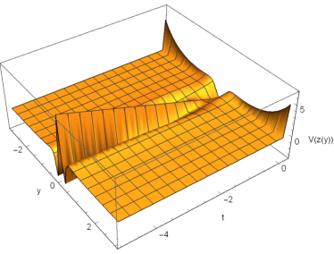
(a) $case$ I

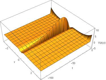
(b) $case$ II

Figure 4: The shapes of the potential $V(z(y))$ for (a) $case$ I and (b) $case$ II. The parameters are set as $a=1$, $b=2$, $c=1$. And in Fig. (a), we set $\mathrm{C}_{1}=\frac{9+10a^{2}}{10a^{2}}$. In Fig. (b), we set $\mathrm{C}_{1}=2$.

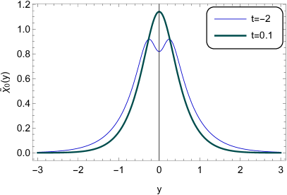
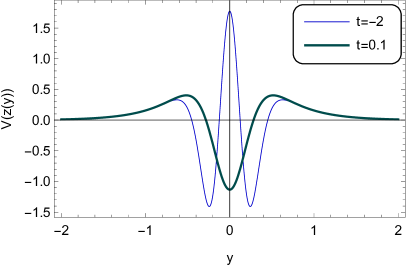
Figure 5: the zero mode $\tilde{\chi}_{0}(y)$ and the effective potential $V(z(y))$ with parameters $a=1,b=2,c=1$ and $\mathrm{C}_{1}=2$. The coupling parameter is set as $t=-2$ for the thin line, and $t=0.1$ for the thick line, respectively.

3.2 dS₄ Brane

In this section, we will discuss the localization of scalar field in the dS₄ brane case. The warp factor considered here takes the form of LiuJCAP20090203

$$e^{2A}=(\cosh(\frac{\beta z}{\delta}))^{-2\delta},$$ (63)

with parameters $0<\delta<1$ and $\beta>0$. This warp factor is of even-parity with respect to coordinate $z$, so we will primarily focus on the asymptotic behaviors of the potential $V(z)$ as $z\rightarrow+\infty$, based on the $\mathbb{Z}_{2}$ symmetry of the braneworld model. Referring to the above expression (63), the scalar curvature (8) has the following solution:

$$R(z)=4(\cosh(\frac{\beta z}{\delta}))^{2\delta}\left(\Lambda+\frac{2\beta^{2}(\textrm{sech}(\frac{\beta z}{\delta}))^{2}}{\delta}-3\beta^{2}(\tanh(\frac{\beta z}{\delta}))^{2}\right).$$ (64)

As $z\rightarrow\infty$, we can get the asymptotic solution for $R$:

$$R(z\rightarrow\infty)\rightarrow(4\Lambda-12\beta^{2})(\cosh(\frac{\beta z}{\delta}))^{2\delta}\rightarrow me^{pz},$$ (65)

with $m=\frac{\Lambda-3\beta^{2}}{4^{\delta-1}}$ and $p=2\beta$ in this subsection, for simplicity. In this context, the value of $m$ determines the asymptotic behavior of the scalar curvature. For $m>0$, the curvature goes to positive infinity asymptotically, while for $m<0$, the curvature tends towards negative infinity when far away from the brane. When $m=0$, the curvature tends to zero, and the bulk spacetime becomes asymptotically flat. In this work, we exclusively consider the case where $m<0$, in which parameters $\Lambda$ and $\beta$ satisfy the relation $\Lambda<3\beta^{2}$. This condition causes the the scalar curvature to tend towards negative infinity as $z\rightarrow\infty$, indicating the presence of singularity of spacetime.

In this case of dS₄ brane, we suggest the function $F(R)$ of the form

$$F(R)=e^{(\ln\mathrm{C}_{1})^{t}-(\ln(\mathrm{C}_{1}-\frac{R}{R_{0}}))^{t}},$$ (66)

where parameters $\mathrm{C}_{1}>2,R_{0}=4(\Lambda+\frac{2\beta^{2}}{\delta})$, and $t$ is the coupling parameter. It is evident that the function $F(R)$ satisfies the normalization condition $F(R\rightarrow 0)=1$. As $z\rightarrow\infty$, the asymptotic solution for $F(R)$ can be given by

$$F(R)\rightarrow we^{-uz^{t}},$$ (67)

with $u=p^{t}$ and $w=e^{(\ln\mathrm{C}_{1})^{t}}$ here.

Then, substituting the warp factor (63) and the asymptotic solution of the function $F(R)$ (67) into the scalar zero mode (40), we can get its asymptotic solution as $z\rightarrow\infty$

$$\tilde{\chi}_{0}(z\rightarrow\infty)\rightarrow N_{2}2^{\frac{3}{2}\delta}w^{\frac{1}{2}}e^{-(\frac{3}{4}pz+\frac{1}{2}uz^{t})}.$$ (68)

The localization of the scalar zero mode requires

$$\int\mathrm{d}z\tilde{\chi}_{0}^{2}(z)<\infty.$$ (69)

From Eq. (68), there is

$$\tilde{\chi}_{0}^{2}(z\rightarrow\infty)\rightarrow N_{2}^{2}2^{3\delta}we^{-(\frac{3}{2}pz+uz^{t})}=N_{2}^{2}2^{3\delta}e^{(\ln\mathrm{C}_{1})^{t}}e^{-3\beta z+(2\beta)^{t}z^{t}}.$$ (70)

It is easy to see that the condition (69) is satisfied without any constraints on a real $t$, thus confirming that the scalar zero mode is normalizable. We present the scalar zero mode in terms of both the coordinate $y$ and $z$ in Fig. 6, with parameters $\delta=0.5,\beta=1,\Lambda=1,\mathrm{C}_{1}=3$, and varying the coupling parameter $t$ with values $2,1$, and $2$, respectively. As shown in the figures, the zero modes in all three cases are localized on the thick brane. Additionally, in the case of $t=-2$, there is a local minimum at the origin of the extra dimension.

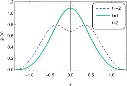
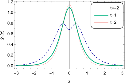
Figure 6: Plots of the scalar zero mode in terms of the coordinate $y$ ($\tilde{\chi}_{0}(y)$ for the left figure) and the coordinate $z$ ($\tilde{\chi}_{0}(z)$ for the right figure) with $\delta=0.5,\beta=1,\Lambda=1$ and $\mathrm{C}_{1}=3$. The coupling parameter is set as $t=-2$ for the dashed line, $t=1$ for the thick line and $t=2$ for the thin line, respectively.

On the other hand, substituting the warp factor (63) and the asymptotic solution of the function $F(R)$ (67) into the effective potential $V(z)$ (36), we can derive its asymptotic solution as $z\rightarrow\infty$:

$$V(z\rightarrow\infty)\rightarrow\frac{9}{4}\beta^{2}+\frac{1}{2}u^{2}t^{2}z^{2(t-1)}+\frac{3}{2}\beta utz^{t-1}.$$ (71)

Therefore, potential $V(z)$ has the following asymptotic behaviors:

$$V(z\rightarrow\infty)\rightarrow\left\{\begin{array}[]{llcll}+\infty&&t&>1\\ \frac{25}{4}\beta^{2}&&t&=1\\ \frac{9}{4}\beta^{2}&&t&<1.\end{array}\right.$$ (72)

Besides, at the location of $z=0$, the effective potential $V(z)$ is

$$V(z=0)=\frac{\beta^{2}\bigg{(}-3\delta+\frac{2t(\delta^{2}-\beta^{2}(2+\delta))\ln(-1+\mathrm{C}_{1})^{-1+t}}{(-1+\mathrm{C}_{1})(2\beta^{2}+\delta)}\bigg{)}}{2\delta^{2}}.$$ (73)

By setting $V(z=0)=0$, we can get

$$case~{}\text{I}: t=\frac{-3\mathrm{C}_{1}+\delta(2\beta^{2}+\delta)}{-2\delta^{2}+2\beta^{2}(2+\delta)},\ \ \ \mathrm{C}_{1}=e+1;$$ (74)

$$case~{}\text{II}: t=\frac{\text{ProductLog}\bigg{[}\mathrm{C}_{2},\frac{3(-1+\mathrm{C}_{1})\delta(2\beta^{2}+\delta)\ln(-1+\mathrm{C}_{1})\ln(\ln(-1+\mathrm{C}_{1}))}{2(\delta^{2}-\beta^{2}(2+\delta))}\bigg{]}}{\ln(\ln(-1+\mathrm{C}_{1}))},$$ (75)

$$\mathrm{C}_{1}\neq e+1\text{ and }\mathrm{C}_{2}\in Integers.$$

The effective potential $V(z)$ for different values of $t$ is depicted in Fig. 7(a) for $case$ I and 7(b) for $case$ II, respectively. In Fig. 7(b), if $V(z=0)=0$, the only real value of $t$ is $-0.846955$, with $\mathrm{C}_{2}=0$ in Eq. (75).

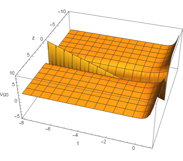
(a) $case$ I

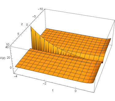
(b) $case$ II

Figure 7: The shapes of the effective potential $V(z)$ for $case$ I and II. The parameters are set as $\delta=0.5,\beta=1,\Lambda=1$. And in Fig. (a), we set $\mathrm{C}_{1}=e+1$. In Fig. (b), we set $\mathrm{C}_{1}=3$.

From the above results, it is clear that the effective potential can be positive at $z=0$ for certain values of $t$. For example, Fig. 8 illustrates the potential $V(z)$ with parameters $\delta=0.5,\beta=1,\Lambda=1,\mathrm{C}_{1}=3$ and the coupling parameter $t=-2,1,2$, respectively. For $t=-2$, the potential possesses a positive maximum at $z=0$, with two negative wells neighboring this potential maximum symmetrically. In contrast, for $t=1$, the effective potential belongs to the Pöschl-Teller-like effective potential; it possesses a negative minimum at $z=0$ and tends to a positive limit when far away from the brane. This type of potential suggests the existence of the mass gap and a series of continuous spectra. Therefore, in addition to the scalar zero mode, finite massive KK modes could be localized on the brane. We describe the localization of these finite massive KK modes in Fig. 9 using numerical methods. The results demonstrate that the potential $V(z)$ belongs to the Pöschl-Teller-like effective potential, and there are three bound states: the ground state (zero mode) $m_{0}^{2}=0$ and two excited states (massive KK modes) $m_{1,2}^{2}=\{4.50,5.58\}$. Finally, for $t=2$, the effective potential $V(z)$ exhibits a negative well at the location of the brane, and its asymptotic behavior is $V(z\rightarrow\infty)\rightarrow+\infty$. Thus, all the massive scalar KK modes are localized on the thick brane.

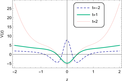
Figure 8: Plots of the effective potential $V(z)$ with $\delta=0.5,\beta=1,\Lambda=1$ and $\mathrm{C}_{1}=3$. The coupling parameter is set as $t=-2$ for the dashed line, $t=1$ for the thick line, and $t=2$ for the thin line, respectively.

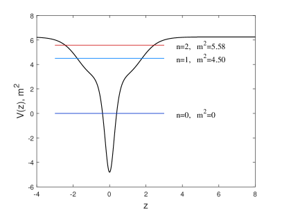
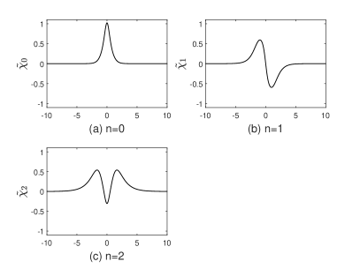
Figure 9: In the left figure, the black line represents the effective potential $V(z)$, and the colored lines represent the positions of mass spectra in the potential. The right figure shows the corresponding solutions of $\tilde{\chi}_{n}(z)$. The parameters are set as $\delta=0.5,\beta=1,\Lambda=1,\mathrm{C}_{1}=3$ and $t=1$.

3.3 AdS₄ Brane

In this section, we will discuss the localization of the scalar field in the case of an AdS₄ brane. The warp factor considered here is of the form SlatyerJHEP2007

$$e^{A(y)}=a\cosh(cy)+b\;\textrm{sech}(cy),$$ (76)

where $a$ and $b$ are dimensionless constants, $c=r\sqrt{\frac{|\Lambda|}{3}}$ with $r$ a positive constant.

By performing the coordinate transformation (6), we can get

$$z(y)=\int e^{-A(y)}dy=\sqrt{\frac{1}{a(a+b)}}\frac{1}{c}\arctan\left[\sqrt{\frac{a}{a+b}}\sinh(cy)\right].$$ (77)

From this expression, it can be seen that coordinate $z\rightarrow\pm\frac{\pi}{2c}\sqrt{\frac{1}{a(a+b)}}$ when $y\rightarrow\pm\infty$, so $z$ has its range $(-z_{max},z_{max})$ with $z_{max}$ defined as

$$z_{max}=\frac{\pi}{2c}\sqrt{\frac{1}{a(a+b)}}.$$ (78)

Inverting Eq. (77), we obtain the expression of $y(z)$:

$$y(z)=\frac{1}{c}~{}\textrm{arcsinh}\left[\sqrt{\frac{a+b}{a}}\tan\left(\sqrt{a(a+b)}\;cz\right)\right].$$ (79)

And the expression of $\text{e}^{A}$ as function of $z$ is:

$$\text{e}^{A(z)}=\frac{\sqrt{a}(a+b)\sec^{2}\left(\sqrt{a(a+b)}\;cz\right)}{\sqrt{a+(a+b)\tan^{2}\left(\sqrt{a(a+b)}\;cz\right)}}.$$ (80)

It is evident that this warp factor is of even-parity with respect to $z$, so we will discuss the asymptotic behaviors of quantities as $z\rightarrow z_{max}$ exclusively.

Substituting this warp factor (80) into the scalar curvature (8), we obtain its asymptotic solution as $z\rightarrow z_{max}$:

$$R(z\rightarrow z_{max})\rightarrow-l(\cos(mz))^{2}-20c^{2},$$ (81)

with $m=\sqrt{a(a+b)}c$ and $l=-(\frac{4\Lambda}{a(a+b)}-\frac{20ac^{2}}{a+b})$ in this subsection.

Here, we suggest the function $F(R)$ takes the form of

$$F(R)=N_{F}e^{2\frac{R+20c^{2}}{l}}(1+\frac{R}{20c^{2}})^{t},$$ (82)

where $N_{F}$ is the normalization constant for $F(R)$, and $t$ is the coupling parameter. The asymptotic solution of $F(R)$ as $z\rightarrow z_{max}$ is

$$F(R)\rightarrow N_{F}e^{2(\cos(mz))^{2}}(\frac{l}{20c^{2}})^{t}(\cos(mz))^{2t}.$$ (83)

By substituting Eq. (83) and Eq. (80) into the scalar zero mode (40), we can obtain its asymptotic solution as follows:

$$\tilde{\chi}_{0}(z\rightarrow z_{max})\rightarrow N_{2}N_{F}(\frac{l}{20c^{2}})^{\frac{1}{2}t}m^{\frac{3}{2}}e^{(\cos(mz))^{2}}(\cos(mz))^{t-\frac{3}{2}}.$$ (84)

As the localization of the scalar zero mode requires

$$\int\mathrm{d}z\tilde{\chi}_{0}^{2}(z)<\infty,$$ (85)

we find that the coupling parameter needs to satisfy

$$t>2.$$ (86)

The scalar zero mode is depicted in terms of both the coordinate $y$ and $z$ in Fig. 10, with parameters $a=0.2,b=0.8,c=2,\Lambda=-3$, and coupling parameter set to $t=2.5,t=3$ and $t=6$, respectively.

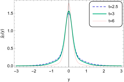
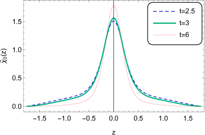
Figure 10: Plots of the zero mode in terms of the coordinate $y$ ($\tilde{\chi}_{0}(y)$ for the left figure) and the coordinate $z$ ($\tilde{\chi}_{0}(z)$ for the right figure) with parameters $a=0.2,b=0.8,c=2,\Lambda=-3$. The coupling parameter is set as $t=2.5$ for the dashed line, $t=3$ for the thick line and $t=6$ for the thin line, respectively.

For the localization of the massive modes, by substituting the asymptotic solution of the function $F(R)$ (83) and the warp factor into the effective potential $V(z)$ (36), we can obtain its asymptotic solution as $z\rightarrow z_{max}$:

$$V(z\rightarrow z_{max})\rightarrow(t-\frac{3}{2})(t-\frac{5}{2})m^{2}\frac{1}{(\cos(mz))^{2}}+\mathrm{C},$$ (87)

where $\mathrm{C}$ is a model-dependent constant. From this expression, together with the condition (86), the effective potential has the following asymptotic behaviors:

$$V(z\rightarrow z_{max})\rightarrow\left\{\begin{array}[]{llcll}+\infty&&t&>\frac{5}{2}\\ \mathrm{C}&&t&=\frac{5}{2}\\ -\infty&&2&<t<\frac{5}{2}.\end{array}\right.$$ (88)

From this expression, we can conclude that the scalar zero mode can be localized when $t>\frac{5}{2}$. However, when $t=\frac{5}{2}$, it depends on the sign of the constant $\mathrm{C}$. If $\mathrm{C}\geq 0$, the scalar zero mode can be localized, but if $\mathrm{C}<0$, it cannot.

The effective potential $V(z)$, with parameters $a=0.2,b=0.8,c=2$, and $\Lambda=-3$, is plotted in Fig. 11 for three different coupling parameters: $t=2.5,t=3$, and $t=6$. In the case of $t=2.5$, the effective potential resembles a Pöschl-Teller-like potential with a positive limit at the boundaries of the brane. This configuration allows for the localization of the scalar zero mode on the brane and provides a mass gap that separates the scalar zero mode from the continuous spectrum of massive modes. Near the brane, two potential barriers appear symmetrically, making it possible to quasi-localize some massive KK modes on the brane.

For $t=3$ and $t=6$, the effective potentials in both cases have similar characteristics, with $V(z\rightarrow\pm z_{max})=\infty$. These properties give rise to the localization of all massive scalar KK modes on the thick AdS₄ brane, forming an infinite discrete mass spectrum. The numerical solutions for lower massive modes are presented in Fig. 12, with parameters $a=1,b=1,c=3,\Lambda=-3$, and $t=3$. The effective potential is oscillator-like, and contains a negative well at the location of the brane, allowing for the localization of both the scalar zero mode and all massive KK modes.

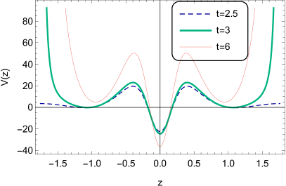
Figure 11: Plots of the effective potential $V(z)$ with parameters $a=0.2,b=0.8,c=2,$ and $\Lambda=-3$. The coupling parameter is set as $t=2.5$ for the thick line, $t=3$ for the dashed line, and $t=6$ for the thin line, respectively.

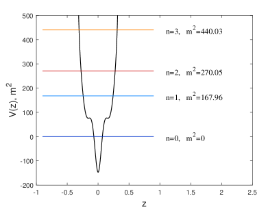
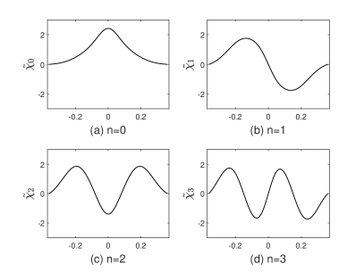
Figure 12: In the left figure, the black line represents the effective potential $V(z)$, and the colored lines represent the positions of the mass spectra. The right figure displays the corresponding solutions of $\tilde{\chi}_{n}(z)$. The parameters are set to $a=1,b=1,c=3,\Lambda=-3$ and $t=3$.

As mentioned earlier, for the coupling parameter $t=2.5$, the potential $V(z)$ is a Pöschl-Teller-like effective potential with two symmetrically located barriers adjacent to the brane. The scalars could tunnel these barriers into the bulk when their 4D squared mass $m^{2}$ satisfy the condition $V_{l}<m^{2}<V_{max}$, where $V_{l}$ represents the limit of the effective potential when far away from the brane, and $V_{max}$ is the maximum of the Pöschl-Teller-like effective potential. And the corresponding massive modes are just the scalar resonances.

In terms of the expression (37), one can interpret $|\tilde{\chi}_{n}(z)|^{2}$ as the probability for finding the massive KK modes at position $z$ along the extra dimension. In Ref. Almeida2009 for the discussion about the fermion resonances, the authors suggests that large peaks in the distribution of $f_{L,R}(0)$ as a function of $m$ would reveal the existence of resonant states. Here, we follow the procedures of the extended idea in Refs. LiuPRD0904 ; ZhaoLMPLA2008 ; LiuPRD2009.80 . For a given eigenvalue $m^{2}$, the corresponding relative probability is defined as:

$$P(m)=\frac{\int^{z_{b}}_{-z_{b}}|\tilde{\chi}(z)|^{2}dz}{\int^{z_{max}}_{-z_{max}}|\tilde{\chi}(z)|^{2}dz},$$ (89)

where $2z_{b}$ is approximately the width of the thick brane, and $z_{max}=10z_{b}$. For these KK modes with larger $m^{2}$ than the maximum of the corresponding potential, they will asymptotically turn into plane waves and the probabilities for them trend to $0.1$. The lifetime $\tau$ of a resonance state is $\tau\sim\Gamma^{-1}$ with $\Gamma=\delta m$ the width of the half height of the resonant peak.

In the model under consideration, we extend the function $F(R)$ (82) to a more general form by introducing an additional coupling parameter $t_{2}$. This extension aims to provide more information regarding the resonance modes. The function $F(R)$ takes the following form:

$$F(R)=N_{F}e^{t_{2}\frac{R+20c^{2}}{l}}(1+\frac{R}{20c^{2}})^{t}.$$ (90)

It is easy to see that the function $F(R)$ (82) is a specific case of this more general expression with the parameter $t_{2}=2$.

Through the same asymptotic analysis as that applied to the form (82), we can observe that incorporating the parameter $t_{2}$ enables us to tune the shapes of the effective potential $V(z)$ at the boundaries of the extra dimension when $t=2.5$. For instance, we plot the effective potential and the corresponding mass spectra in Fig. 13(a), along with the relative probabilities $P$ in Fig. 13(b). The chosen parameters are $a=0.2,b=0.8,c=1.25,t=2.5$ and $t_{2}=100$. It should be noted that in Fig. 13(a), the effective potential $V(z)$ does not tend to zero at the boundaries of the extra dimension. From Fig. 13(b), we can discern the presence of four resonance peaks, each corresponding to a resonance state. Analyzing the mass spectra of scalars, it is apparent that the ground state represents the scalar zero mode (bound state), and the four lower massive KK modes are resonance KK modes. The shapes of these scalar resonances are displayed in Fig. 14. These figures illustrate that as the corresponding mass increases, the shapes of resonance KK modes trend to be plane waves, indicating increased possibility for tunnelling. Additionally, Table 1 provides information on the width $\Gamma$, lifetime $\tau$ and relative probability $P$ of all resonance KK modes. Notably, resonance modes with lower mass exhibit higher relative probabilities and longer lifetimes for existing on the thick brane.

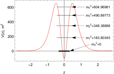
(a) $V(z),m^{2}$

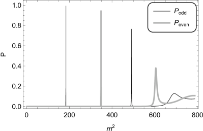
(b) $P$

Figure 13: (a) The effective potential $V(z)$ and the mass spectra. (b) The corresponding relative probability $P$. The parameters are set as $a=0.2,b=0.8,c=1.25,t=2.5$, and $t_{2}=100$. In Fig. (a), the red thin line is for the potential $V(z)$.

Figure 14: The shapes of resonance KK modes $\tilde{\chi}(z)$ for scalars with different $m^{2}$. The parameters are set as $a=0.2,b=0.8,c=1.25,t=2.5$ and $t_{2}=100$.

Table 1: The mass, width, lifetime and relative probability for scalar resonances. The parameters are set as $a=0.2,b=0.8,c=1.25,t=2.5$ and $t_{2}=100$.

	$m^{2}$	$m$	$\Gamma$	$\tau$	$P$
$n=1$	183.80345	13.55741	0.00000284	351789.9	0.99416
$n=2$	348.38888	18.66518	0.0004647	2151.84	0.94869
$n=3$	490.89773	22.15621	0.01730	57.8072	0.76369
$n=4$	604.96981	24.59613	0.21662	4.61627	0.37877

4 Conclusions

In this paper, we consider a general coupling mechanism between the kinetic term and the spacetime. There is a factor $F(R)$ which is a function of scalar curvature of the bulk in the five-dimensional action for scalars. Based on this scenario, we explore the localization of the scalar field on specific braneworld models characterized by three different types of brane geometries: Minkowski, dS₄, and AdS₄. Besides, scalar resonances in the case of AdS₄ brane are also discussed.

In the case of a Minkowski brane, we can observe three typical types of effective potentials: volcanic-like, Pöschl-Teller-like, and the infinitely deep well, respectively, which are determined by the coupling parameter $t$. Initially, the scalar zero mode will be normalizable when with a real $t$. For $t<\frac{1}{6}a^{2}$, only the scalar zero mode can be localized on the brane, resulting in the volcanic-like effective potential. When certain negative values of $t$ are present, the effective potential will possess a positive maximum at the origin of the extra dimension. For $t=\frac{1}{6}a^{2}$, there will be a Pöschl-Teller-like effective potential. The localized zero mode will be separated from a series of continuous spectra of massive ones by a mass gap. For $t>\frac{1}{6}a^{2}$, the effective potential tends towards infinity when far away from the brane. A special case resembles the one-dimensional quantum harmonic oscillator problem.

In the dS₄ brane case, the scalar zero mode is normalizable when $t$ is real. Then, for $t<1$, the effective potentials have the asymptotic behavior: $V(z\rightarrow\infty)\rightarrow\frac{9}{4}\beta^{2}$, and maintain a positive maximum at $z=0$ for specific values of the coupling parameter $t$. When $t=1$, the effective potential is the Pöschl-Teller-like effective potential, and trends to the limit $\frac{25}{4}\beta^{2}$ when far away from the brane. Consequently, finite massive scalar KK modes as well as the scalar zero mode can be trapped on the thick brane. Lastly, for $t>1$, the effective potential takes the form of an infinitely deep well, supporting infinite bound KK modes.

In the case of an AdS₄ brane, we can obtain Pöschl-Teller-like effective potentials and infinitely deep wells as the coupling parameter $t$ varies. When $t=2.5$, the effective potential approaches a constant limit $\mathrm{C}$ at the boundaries of the brane. If $\mathrm{C}\geq 0$, the scalar zero mode can be localized. Simultaneously, within the effective potential, two potential barriers are symmetrically positioned near the brane. By extending the function $F(R)$ and introducing another coupling parameter $t_{2}$, scalar resonances can emerge. For $t>2.5$, an infinitely deep well forms, including a negative well at the location of the brane. In this case, both the scalar zero mode and the massive modes can be localized on the thick brane.

References

- (1) V.A. Rubakov and M.E. Shaposhnikov, Phys. Lett. B 125 (1983) 136; V.A. Rubakov and M.E. Shaposhnikov, Phys. Lett. B 125 (1983) 139;
- (2) M. Visser, Phys. Lett. B 159 (1985) 22.
- (3) K. Akama, Lect. Notes Phys. 176 (1983) 267; C. Wetterich, Nucl. Phys. B 253 (1985) 366; S. Randjbar-Daemi and C. Wetterich, Phys. Lett. B 166 (1986) 65.
- (4) J. Lykken and L. Randall, JHEP 0006 (2000) 014.
- (5) I. Antoniadis, Phys. Lett. B 246 (1990) 377.
- (6) L. Randall and R. Sundrum, Phys. Rev. Lett. 83 (1999) 3370; Phys. Rev. Lett. 83 (1999) 4690.
- (7) T. Appelquist, A. Chodos and P.G.O. Freund, Modern KaluzaKlein Theories, Addison-Wesley Publishing Company, Boston, (1987).
- (8) I. Antoniadis, A. Arvanitaki, S. Dimopoulos and A. Giveon, Phys. Rev. Lett. 108 (2012) 081602.
- (9) K. Yang, Y.-X. Liu, Y. Zhong, X.-L. Du and S.-W. Wei, Phys.Rev.D 86 (2012) 127502.
- (10) I. Antoniadis, N. Arkani-Hamed, S. Dimopoulos and G. Dvali, Phys. Lett. B 436 (1998) 257.
- (11) N. Arkani-Hamed, S. Dimopoulos and G. Dvali, Phys. Lett. B 429 (1998) 263.
- (12) O. DeWolfe, D.Z. Freedman, S.S. Gubser and A. Karch, Phys. Rev. D 62 (2000) 046008.
- (13) K. Ghoroku and M. Yahiro, hep-th/0305150; A. Kehagias and K. Tamvakis, Mod. Phys. Lett. A 17 (2002) 1767; Phys. Lett. B 504(2001) 38; M. Giovannini, Phys. Rev. D 64 (2001) 064023; Phys. Rev. D 65 (2002) 064008.
- (14) C. Csaki, J. Erlich, T. Hollowood and Y. Shirman, Nucl. Phys. B 581 (2000) 309.
- (15) A. Wang, Phys. Rev. D 66(2002) 024024.
- (16) V. Dzhunushaliev, V. Folomeev, D. Singleton and S. Aguilar-Rudametkin, Phys. Rev. D 77 (2008) 044006; V. Dzhunushaliev, V. Folomeev, K. Myrzakulov and R. Myrzakulov, Gen. Rel. Grav. 41 (2008) 131; D. Bazeia, F.A. Brito and J.R. Nascimento, Phys. Rev. D 68 (2003) 085007; D. Bazeia, F.A. Brito and A.R. Gomes, JHEP 0411 (2004) 070; D. Bazeia and A.R. Gomes, JHEP 0405 (2004) 012; D. Bazeia, A.R. Gomes and L. Losano, Int. J. Mod. Phys. A 24 (2009) 1135.
- (17) D. Bazeia, F.A. Brito and L. Losano, JHEP 0611 (2006) 064; V.I. Afonso, D. Bazeia and L. Losano, Phys. Lett. B 634 (2006) 526.
- (18) A. Herrera-Aguilar, D. Malagon-Morejon, R.R. Mora-Luna and U. Nucamendi, Mod. Phys. Lett. A25 (2010) 2089.
- (19) Y.-X. Liu, K. Yang and Y. Zhong, JHEP 1010 (2010) 069.
- (20) Y.-X. Liu, Y. Zhong and K. Yang, Europhys. Lett. 90 (2010) 51001.
- (21) Y. Zhong, Y.-X. Liu and K. Yang, Phys. Lett. B 699 (2011) 398.
- (22) H. Guo, Y.-X. Liu, S.-W. Wei and C.-E. Fu, Europhys. Letters 97 (2012) 60003.
- (23) A. Herrera-Aguilar, D. Malagon-Morejon and R.R. Mora-Luna, JHEP 1011 (2010) 015.
- (24) T.R. Slatyer and R.R. Volkas, JHEP 0704 (2007) 062.
- (25) Y.-X. Liu, H. Guo, C.-E. Fu and H.-T. Li, Phys. Rev. D 84 (2011) 044033.
- (26) Y. Zhong and Y.-X. Liu, Eur. Phys. J. C 76 (2016) 321.
- (27) Y. Zhong, Y. Zhong, Y.-P. Zhang and Y.-X. Liu, Eur. Phys. J. C 78 (2018) 45.
- (28) G. German, A. Herrera-Aguilar, D. Malagon-Morejon, R.R. Mora-Luna and R. da Rocha, JCAP 1302 (2013) 035.
- (29) A. Pomarol, Phys. Lett. B 486 (2000) 153.
- (30) P. Jones, G. Munoz, D. Singleton and Triyanta, Phys. Rev. D 88 (2013) 025048.
- (31) L.J.S. Sousa, C.A.S. Silva and C.A.S. Almeida, Phys. Lett. B 718 (2013) 579.
- (32) S.G. Rubin, Eur. Phys. J. C 75 (2015) 333.
- (33) T. Gherghetta and A. Pomarol, Nucl. Phys. B 586 (2000) 141.
- (34) D. Youm, Nucl. Phys. B 589 (2000) 315.
- (35) H. Abe, T. Kobayashi, N. Maru and K. Yoshioka, Phys. Rev. D 67 (2003) 045019.
- (36) K. Ghoroku and M. Yahiro, Class. Quant. Grav. 20 (2003) 3717.
- (37) I. Oda, Phys. Lett. B 571 (2003) 235.
- (38) Y.-X. Liu, X.-H. Zhang, L.-D. Zhang and Y.-S. Duan, JHEP 0802 (2008) 067.
- (39) K. Ghoroku and A. Nakamura, Phys. Rev. D 65 (2002) 084017.
- (40) I.C. Jardim, G. Alencar, R.R. Landim and R. Costa Filho, Phys. Rev. D 91 (2015) 085008.
- (41) Z.-H. Zhao and Q.-Y. Xie, JHEP 05 (2018) 072.
- (42) B. Bajc and G. Gabadadze, Phys. Lett. B 474 (2000) 282.
- (43) Y.-X. Liu, L.-D. Zhang, S.-W. Wei and Y.-S. Duan, JHEP 0808 (2008) 041.
- (44) I. Oda, Phys. Lett. B 496 (2000) 113.
- (45) Y.-X. Liu, J. Yang, Z.-H. Zhao, C.-E. Fu and Y.-S. Duan, Phys. Rev. D 80 (2009) 065019.
- (46) C.A.S. Almeida, R. Casana, M.M. Ferreira Jr. and A.R. Gomes, Phys. Rev. D 79 (2009) 125022.
- (47) W.T. Cruz, L.J.S. Sousa, R.V. Maluf and C.A.S. Almeida, Phys. Lett. B 730 (2014) 314.
- (48) Z.-G. Xu, Y. Zhong, H. Yu and Y.-X. Liu, Eur. Phys. J. C 75 (2015) 368.
- (49) C. Csaki, J. Erlich and T.J. Hollowood, Phys. Rev. Lett. 84, (2000) 5932.
- (50) Y.-P. Zhang, Y.-Z. Du, W.-D. Guo and Y.-X. Liu, Phys. Rev. D 93 (2016) 065042.
- (51) Y. Zhong, Y. Zhong, Y.-P. Zhang and Y.-X. Liu, Eur. Phys. J. C. 78 (2018) 45.
- (52) W.-D. Guo, Y. Zhong, K. Yang, T.-T. Sui and Y.-X. Liu, Phys. Lett. B 800 (2020) 135099.
- (53) T.-T. Sui, W.-D. Guo, Q.-Y. Xie and Y.-X. Liu, Phys. Rev. D 101 (2020) 055031.
- (54) Q. Tan, W.-D. Guo, Y.-P. Zhang and Y.-X. Liu, Eur. Phys. J. C 81 (2021) 373.
- (55) J. Chen, W.-D. Guo and Y.-X. Liu, Eur. Phys. J. C 81 (2021) 709.
- (56) Q. Tan, Y.-P. Zhang, W.-D. Guo, J. Chen, C.-C. Zhu and Y.-X. Liu, Eur. Phys. J. C 83 (2023) 84.
- (57) J. Barranco, A. Bernal, J.C. Degollado, et al., Phys. Rev. D 84 (2011) 083008.
- (58) J. Barranco, A. Bernal, J.C. Degollado, et al., Phys. Rev. Lett. 109 (2012) 081102.
- (59) J. Barranco, A. Bernal, J.C. Degollado, et al., Phys. Rev. D 89 (2014) 083006.
- (60) X.-N. Zhou, X.-L. Du, K. Yang and Y.-X. Liu, Phys. Rev. D 89 (2014) 043006.
- (61) G.H. Gossel, J.C. Berengut and V.V. Flambaum, Int. J. Mod. Phys. D 23 (2014) 1450089.
- (62) M.O.P. Sampaio, C. Herdeiro and M. Wang, Phys. Rev. D 90 (2014) 064004.
- (63) J.C. Degollado and C.A.R. Herdeiro, Phys. Rev. D 90 (2014) 065019.
- (64) N. Sanchis-Gual, J.C. Degollado, P.J. Montero and J.A. Font, Phys. Rev. D 91 (2015) 043005; N. Sanchis-Gual, J.C. Degollado, P.J. Montero, J.A. Font and V. Mewes, Phys. Rev. D 92 (2015) 083001; N. Sanchis-Gual, J.C. Degollado, P. Izquierdo, J.A. Font and P.J.Montero, Phys. Rev. D 94 (2016) 0430004.
- (65) Y. Huang, D.-J. Liu, X.-H. Zhai and X.-Z. Li, Phys. Rev. D 96 (2017) 065002.
- (66) C.A. Sporea, Mod. Phys. Lett. A 34 (2019) 1950323.
- (67) P.W. Higgs, Phys. Lett. 12 (1964) 132.
- (68) P.W. Higgs, Phys. Rev. Lett. 13 (1964) 508.
- (69) ATLAS Collaboration, Phys. Lett. B 716 (2012) 1-29.
- (70) B. Mukhopadhyaya, S. Sen and S. SenGupta, Phys. Rev. D 76 (2007) 121501.
- (71) F. Quevedo, S. Krippendorf and O. Schlotterer, Cambridge lectures on supersymmetry and extra dimensions, arXiv: 1011.1491.
- (72) J. Liang and Y.-S. Duan, Phys. Lett. B 678 (2009) 491.
- (73) H. Guo, L.-L. Wang, C.-E. Fu and Q.-Y. Xie, Phys. Rev. D 107 (2023) 104017.
- (74) A. Flachi and M. Minamitsuji, Phys. Rev. D 79 (2009) 104021.
- (75) J. Liang and Y.-S. Duan, Phys. Lett. B 680 (2009) 489.
- (76) Y.-X. Liu, Z.-H. Zhao, S.-W. Wei and Y.-S. Duan, JCAP. 0902 (2009) 003.
- (77) H. Guo, A. Herrera-Aguilar, Y.-X. Liu, et al., Phys. Rev. D 87(2013) 095011.
- (78) Y.-X. Liu, H. Guo, C.-E. Fu and J.-R. Ren, JHEP 1002 (2010) 080.
- (79) R. Davies and D. P. George, Phys. Rev. D 76 (2007) 104010; D. P. George and R. R. Volkas, Phys. Rev. D 75 (2007) 105007.
- (80) L. Zhao, Y.-X. Liu and Y.-S. Duan, Modern Physics Letters A 23 (2008) 1129.
- (81) Y.-X. Liu, C.-E. Fu, L. Zhao and Y.-S. Duan, Phys. Rev. D 80 (2009) 065020.