Elastic Interaction Energy Loss for
Traffic Image Segmentation

Abstract

Segmentation is a pixel-level classification of images. The accuracy and fast inference speed of image segmentation are crucial for autonomous driving safety. Fine and complex geometric objects are the most difficult but important recognition targets in traffic scene, such as pedestrians, traffic signs and lanes. In this paper, a simple and efficient geometry-sensitive energy-based loss function is proposed to Convolutional Neural Network (CNN) for multi-class segmentation on real-time traffic scene understanding. To be specific, the elastic interaction energy (EIE) between two boundaries will drive the prediction moving toward the ground truth until completely overlap. The EIE loss function is incorporated into CNN to enhance accuracy on fine-scale structure segmentation. In particular, small or irregularly shaped objects can be identified more accurately, and discontinuity issues on slender objects can be improved. Our approach can be applied to different segmentation-based problems, such as urban scene segmentation and lane detection. We quantitatively and qualitatively analyze our method on three traffic datasets, including urban scene data Cityscapes, lane data TuSimple and CULane. The results show that our approach consistently improves performance, especially when using real-time, lightweight networks as the backbones, which is more suitable for autonomous driving.

1 Introduction

Semantic segmentation is a pixel-level classification of images, which is one of the most important tasks in computer vision. It is widely used in the field of autonomous driving perception, such as urban scene segmentation, lane detection and 3D reconstruction. In the urban scene, accurate multi-class semantic segmentation is needed to distinguish the drivable areas (roads) from sidewalks, buildings, vehicles, pedestrians, traffic signs, etc. In the lane detection problem, the existence and location of lane boundaries need to be inferenced in real time, even when they are occluded.

At present, vast studies of image segmentation problem focus on the improvement of neural network structure, such as deeper and denser networks and attention-based methods like vision-transformer. Although complex network structure with tons of parameters promise sophisticated performance, it would also cause large computational cost and relatively slow reasoning speed, which is inconvenient for the field of autonomous driving that requires real-time perception under limit computing resource. On the other hand, because prediction errors often appear on geometry complex objects, such as missing or disconnected at slender structures with just a few pixel inside and blurry on boundaries of irregular shapes, another prevailing direction is to develop boundary-aware loss function according to geometry relation between the prediction and ground truth. The main branch of the boundary refinement method is post processing, which will slow the inference speed. Another type of methods consider the similarity of the boundaries between prediction and ground truth, but still not consider them as a whole using cross entropy as the evaluation metric, so still not sensitive enough to objects containing just a few pixels. The uniqueness of our method is that we provide a novel measurement on distance between boundaries that has long range relation. Our method focus more on fine-scale structures.

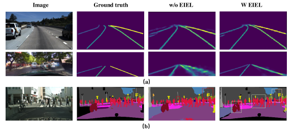
Figure 1: Comparison of the output maps between Baseline ERFNet  [1] with or without EIEL in (a) lane detection and (b) segmentation. To be specific, the pictures from left to right are: raw image, ground truth, outputs without / with our loss.

We propose a geometry-aware loss function, elastic interactrion energy loss (EIEL) in multi class semantic segmentation, and named the training strategy as EIEGSeg (EIE Guided Segmentation) to improve the segmentation effect of complex geometries under class imbalance. Our loss function is inspired by the line defects of dislocation in crystal. In image processing problems, this energy considers pixel sets on boundary of an object as a whole, rather than summation of distance between pairwise pixels, so long-thin objects tend to be connected when the energy descents, and the boundaries on thin concave or convex area also perform well. Our strategy will not lead to increase to computational complexity and inference time comparing to the baseline. We believe that this loss function is also working in larger size models on other application such as high resolution image segmentation.

The proposed strategy EIEGSeg is jointly trained by the guidance of EIEL and cross entropy (CE). In multi class learning, $N$ class of feature maps are output at the last layer of neural network. The EIEGSeg employs the level set method via the predicted output maps $P$, where the position of $P-0.5=0$ can implicitly express the boundaries function of the predicted region. CE can help predict the coarse class distribution on pixels, and EIEL enforces the boundaries of these predicted regions of different classes moving toward the one-hot ground truth, thus the predicted area could be more perfectly fit the actual region. Figure 1 shows some effective applications by adding EIEL on a baseline. Slender objects such as poles and occluded lane lines are better connected and identified, boundaries of small and irregular shape objects such as traffic sign, traffic light, pedestrians, riders, etc. would be clearer recognized.

We evaluate our method on three popular autonomous driving scene benchmarks, including two lane detection datasets, i.e. Tusimple and CULane, and one urban scene data Cityscapes. We compare the performance based on a lightweight network structure ERFNet, BiSeNetV1, and a state-of-the-art FCN semantic segmentation baseline HRNet-W48-OCR, with or without EIEL function. The experiment results show that adding EIEL can indeed improve the accuracy, F1-score and mIoU.

The main contributions are as follow:

• We propose a simple and efficient geometry sensitive energy-based loss function EIEL for multi class segmentation for real-time traffic scene understanding. Small or irregularly shaped objects can be identified more accurately, and discontinuity issues on slender objects can be significantly improved.

• The EIEGSeg can achieve end-to-end segmentation and works well on both lightweight and high resolution network backbones, especially on lightweight one to make real-time inference.

• Three datasets are used to evaluate our method. In TuSimple and CULane, the lane segmentation is much clearer and disconnection casued by occlusion is fixed. In Cityscapes, the prediction accuracy on fine-scale structure objects increase significantly.

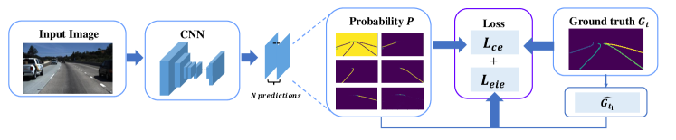
Figure 2: Architecture of EIEGSeg.

2 Related Work

2.1 Semantic Segmentation Architecture

The fast development of end-to-end segmentation started from fully convolutional network (FCN)  [2]. Many following works are based on this network structure, which including several down-sampling and upsampling steps. Some networks have deeper and denser layers, such as  [3], some have smaller backbones with light parameters like  [1, 4, 5, 6] can achieve real-time performance become to balance effectiveness and efficiency. In lane segmentation problems, novel spatial information passing strategies were also proposed, e.g., SCNN  [7]. Recently, network architectures have been developed that take into account of both performance and speed, such as  [8] with dilated convolutions,  [9] and  [10] having good feature fusion capability by ingenious blocks-connection schemes.

2.2 Geometry-aware segmentation

There are two branches of segmentation refinement, i.e., post-processing and applying geometry-aware loss function.

Post-refinement such as markov random fields (MRF)  [11] and conditional random fields (CRFs)  [12] were studied to refine the outputs of network. Clustering is utilized to distinguish the instances type in lane detection task after training. Segfix  [13] can transfer the interior pixels to be boundaries by training a separate network.

Some works on segmentation geometry focus on boundary. Pairwise pixel-level affinity fields can be used to classify different pixels, e.g.  [14, 15]. InverseForm  [16], a structured boundary-aware segmentation method, gave a novel boundary-aware loss using an inverse-transformation network. These training process also combined with cross-entropy using multi-task learning (MTL) and fuse the sub-branch features to the main-branch segmentation to improve the details. However, they are not sensitive in long thin objects. ABL  [17] and BL  [18] are proposed to refine the boundary details.

Others focus on topology relation of pixels. Intersection over union (IoU) was transformed into differentiable form loss function to guide the refinement of pixels prediction  [19].  [20, 21] utilized elastic interaction energy loss function to achieve connection improvement on medical binary segmentation. The closest training strategy to ours is  [22], which uses a topology-preserving loss function based on the thought of level set method and Betti number in conjunction with CE to ensure the connectivity of slender objects, but it can just be applied in binary problems, e.g. eye blood vessels, remote sensing data and road crack segmentation.

3 Method

3.1 Network Structure

We implemented two segmentation-based image processing tasks, the semantic segmentation in urban scene and the instance lane segmentation. The overall training strategies are the similar. The overall architecture of EIEGSeg is showed in figure 2. In semantic segmentation problem, we upsample the feature size and get end-to-end pixelwise prediction. The size of input images are H and W, and the output is with the size of $B*C*h*w$, where $C$ is the number of output feature map, $h=H/s$, $w=W/s$. The ground truth is adjusted into one-hot form while applying EIEL. In lane detection problems, we upsample the features into $1/4$ as the original size, i.e. $B*C*h*w$ where $s=4$, because lanes are well structured, and do not need so many pixels to represent them. The ground truth is also down-scale to $1/4$ with linear interpolation. After segmentation, we chose the pixels in the center each row of the lane line as their coordinates. Thus the problem is equivalently to sampling equidistant on the y axis and choosing the x coordinate based on the probability output.

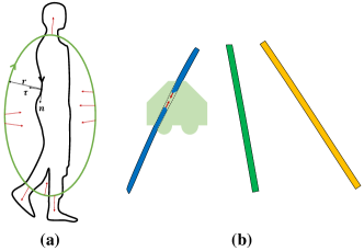
Figure 3: Description of how the EIEL works. (a) shows how the moving curve being attracted to the ground truth. (b) shows how the disconnected prediction of the left most lane can be corrected by EIEL even it is occluded by a car.

3.2 Elastic interaction energy loss (EIEL)

The elastic interaction energy functional is

$$E =E_{s}+E_{i}$$ (1)

$$=\frac{1}{8\pi}\int_{\gamma_{gt}\cup\gamma_{p}}\int_{\gamma_{gt}^{\prime}\cup\gamma_{p}^{\prime}}\frac{d\boldsymbol{l}\cdot d\boldsymbol{l}^{\prime}}{r}$$

$$=\frac{1}{8\pi}\int_{\gamma_{gt}}\int_{\gamma_{gt}^{\prime}}\frac{d\boldsymbol{l}_{\mathbf{gt}}\cdot d\boldsymbol{l}_{\mathbf{gt}}^{\prime}}{r}+\frac{1}{8\pi}\int_{\gamma_{p}}\int_{\gamma_{p}^{\prime}}\frac{d\boldsymbol{l}_{\mathbf{p}}\cdot d\boldsymbol{l}_{\mathbf{p}}^{\prime}}{r}$$

$$\quad+\frac{1}{4\pi}\int_{\gamma_{gt}}\int_{\gamma_{p}}\frac{d\boldsymbol{l}_{\mathbf{gt}}\cdot d\boldsymbol{l}_{\mathbf{p}}}{r}$$

In the above functional, $\gamma^{\prime}$ is the curves with other parameter $s^{\prime}$, vector $d\boldsymbol{l}$ represents line element on one set of curves $\gamma$ with tangent direction $\boldsymbol{\tau}$, i.e. $d\boldsymbol{l}=\boldsymbol{\tau}dl$, and the $r$ is Euclidean distance between (x,y) and ($\left.\mathrm{x}^{\prime},\mathrm{y}^{\prime}\right)$, i.e. $r=$ $\sqrt{\left(x-x^{\prime}\right)^{2}+\left(y-y^{\prime}\right)^{2}}$. The vector $\boldsymbol{l}$ as the sum of ground truth $\boldsymbol{l_{gt}}$ and the predicted $\boldsymbol{l_{p}}$, and their directions are opposite, $\boldsymbol{l}=\boldsymbol{l_{gt}}+\boldsymbol{l_{p}}$.

In Eq. (1), the self-energy $E_{s}$ consists of the first two terms for the self-energies of the prediction curve set $\gamma_{p}$ and the ground truth curve set $\gamma_{gt}$, while the third term is the interaction energy $E_{i}$ between the two sets of curves $\gamma_{p}$ and $\gamma_{gt}$. Since the prediction curve $\gamma_{p}$ and the ground truth curve $\gamma_{gt}$ have opposite orientations, the elastic interaction between them is strongly attractive based on the third term in Eq. (1), and the prediction curve $\gamma_{p}$ is attracted to the ground truth curve $\gamma_{gt}$ to minimize the total energy in Eq. (1); see Fig. 3(a). When the two curves coincide, the energy minimum state is reached, and the ground truth is identified perfectly by the prediction. Under this elastic energy, the boundaries of the disconnected parts of the prediction are also attracted to each other for the same reason, and eventually combine; see Fig. 3(b). Besides, the self-energy of the prediction tends to make the prediction curves smoothing, because a longer curve has a larger self-energy. More mathematical properties of this elastic loss can be found in  [20, 21].

In the image space, the curves can be implicitly ex-pressed by gradient of pixels, i.e. $\nabla G_{t}=-\delta(\gamma_{gt})\boldsymbol{n}$ for ground truth $G_{t}$ and $\nabla H(\phi)=-\delta(\gamma_{p})\boldsymbol{n}$ for prediction.

Thus, the elastic interaction energy as well as the EIE loss function should be:

$$\begin{split}&L_{eie}=\frac{1}{8\pi}\int_{\mathbf{R}^{2}}dxdy\\ &\int_{\mathbf{R}^{2}}\frac{\nabla\left(G_{t}+\alpha H(\phi)\right)(x,y)\cdot\nabla\left(G_{t}+\alpha H(\phi)\right)\left(x^{\prime},y^{\prime}\right)}{r}dx^{\prime}dy^{\prime}\end{split}$$ (2)

3.3 Efficient calculation

As the energy function $L_{eie}$ in Eq. (2) is an integral over the whole image domain, fast Fourier transform can make the computation more efficiently. Assume the Fourier transform of $G_{t}+\alpha H(\phi(x,y))$ is $d_{mn}$, where $m$ and $n$ are frequencies in the Fourier space. The Fourier transform of

$$\frac{1}{R}=\frac{1}{\sqrt{x^{2}+y^{2}}}\text{ is }\frac{\widehat{1}}{R}=\frac{1}{2\pi\sqrt{m^{2}+n^{2}}}.$$

Therefore, in the Fourier space, the EIEL can be transformed into the form as

$$L_{eie}=\sum_{m,n}\sqrt{m^{2}+n^{2}}\cdot\left|d_{mn}\right|^{2}.$$ (3)

Then the Fourier transform of the variation of EIEL $L_{eie}$ should be expressed as

$$\frac{\widehat{\partial L_{eie}}}{\partial\phi}=\frac{\sqrt{m^{2}+n^{2}}}{2}d_{mn}.$$

Thus the gradient of $L_{eie}$ is the inverse Fourier transform, which is used in backward propagation

$$\frac{\partial L_{eie}}{\partial\phi}=\mathcal{F}^{-1}\left(\frac{\sqrt{m^{2}+n^{2}}}{2}d_{mn}\right).$$ (4)

3.4 Multi class segmentation via EIEL

In $N$ class semantic segmentation, every pixel on an image has a class label from 0 to $N-1$. Some times, the background is one of the classes (class 0 in lane detection task, but classed as ignore-label 255 in segmentation task). Therefore, the output layer has N feature prediction maps, i.e. the output size is $B*N*h*w$.
In our method, the boundaries of each class of objects are modeled as the zero level set of different level set functions $\phi_{i}(x,y)$, i is the ith class of object. As the prediction on each pixel is presented as probability distribution, the value would be within [0,1]. Each output map is represented with $P_{i}$ and Softmax is applied to convert it into a pixel probability maps, i.e. $\sigma:P\rightarrow[0,1]^{N*h*w}$, then the level set function of predictions would be

$$\phi_{i}=\sigma(P)_{i}-0.5,$$ (5)

and the corresponding expression of ground truth with opposite orientation is

$$\phi_{i}*=0.5-\hat{{G_{t}}_{i}},$$ (6)

where $\hat{{G_{t}}_{i}}$ is the one-hot mode of the ground truth,

$$\hat{G}_{t_{i}}=\mathbf{1}_{G_{t_{i}}},$$

The training loss $L_{t}$ in EIEGSeg is

$$L_{l}=\lambda_{1}\sum_{i}L_{\text{eie }}(\sigma(P)_{i},\hat{{G_{t}}_{i}})+\lambda_{2}L_{ce}\left(P,G_{t}\right).$$ (7)

where $L_{eie}$ represents EIE loss and $L_{ce}$ is the cross-entropy loss.

4 Experiments

The experiments are implemented on a GPU RTX 4000 and RTX 3060. We apply our EIEL on segmentation dataset Cityscapes and two lane-detection datasets Tusimple and CULane. In Cityscapes, dense annotations with 19 object classes are provided. The training and validation data amount is 2975 and 500, and we use the validation data in testing. In lane datasets, lanes coordinates are provided officially. Tusimple has a maximum of five lane lines on highway and most of which are in daytime and clear weather, which concludes 3626 training data (we separate 3268 for train and 358 for validation) and 2782 testing data. CULane includes eight difficult-to-detect urban environments such as crowded, darkness, no-line, and shadows, and marks up to four lane lines. Data volume is 88880/9675/34680 as train/val/test.

Method	road	side -walk	building	wall	fence	pole	traffic light	traffic sign	vegetation	terrian	sky	person	rider	car	truck	bus	train	motor	bicycle	mIoU
ERFNet	97.46	80.79	90.28	49.5	55.6	60.46	61.48	70.33	91.07	61.65	93.3	74.12	54.5	92.14	62.24	73.55	60.34	45.18	68.44	70.65
ERFNet+EIEL	97.69	80.46	91.57	58.48	53.19	65.36	66.86	74.69	92.21	63.86	94.06	78.72	59.76	93.66	71.08	77.68	64.93	46.55	72.1	73.84
BiSeNetV1	97.93	83.42	91.70	47.21	52.44	63.13	70.41	77.76	91.99	61.64	94.73	80.64	59.60	94.50	73.23	83.25	74.07	58.34	75.96	75.37
BiSeNetV1+EIEL	98.05	84.45	92.42	55.27	59.05	65.52	70.97	78.84	92.38	63.48	94.92	81.40	61.80	94.52	66.47	79.43	72.82	52.53	76.43	75.83
OCR	98.52	87.5	93.67	62.15	66.47	71.6	75.48	82.62	93.32	66.31	95.04	84.69	66.76	95.90	86.58	91.59	86.58	69.39	79.70	81.60
OCR+EIEL	98.44	87.3	93.54	63.27	65.81	72.3	75.71	83.71	93.08	65.51	94.78	85.19	69.33	95.91	85.15	88.87	84.49	69.80	80.12	81.70
OCR(MS)	98.61	88.11	93.94	65.67	67.51	72.67	77.00	84.05	93.58	67.75	95.11	85.66	68.44	96.24	88.05	92.73	86.13	71.16	80.91	82.80
OCR+EIEL(MS)	98.61	88.39	93.94	66.71	68.37	73.95	77.67	85.06	93.45	69.26	95.00	86.38	71.12	96.20	81.36	91.61	84.99	71.53	81.39	82.90

Table 1: Class-wise mIoU results from single-scale inference on Cityscapes validation set. OCR refers to the backbone HRNet-W48-OCR. The results are according to our implementation. MS means the results of multi-scale inference.

4.1 Evaluation Metrics

4.1.1 Cityscapes.

We apply the official metric mean Intesection-over-Union (mIoU) and the IoU of each class to measure the performance overall and in specific categories.

4.1.2 TuSimple.

The official metric of the TuSimple dataset is accuracy (Acc), the false positive (FP) and the false negetive (FN). In addition to this, we also evaluate the average pixelwise F1 score (Pix. F1). The accuracy of TuSimple accuracy is:

$$\text{ Accuracy }=\frac{N_{pred}}{N_{gt}}$$ (8)

where $N_{pred}$ is the number of correct predicted lane points and $N_{gt}$ is the amount of ground-truth lane points.

4.1.3 CULane.

The officially metric for CULane is F1 measure (F1-score) based on Intersection over Union (IoU):

$$F1=2\cdot\left(\frac{precision\cdot recall}{precision+recall}\right)$$ (9)

where $precision$ defined as $\frac{TP}{TP+FP}$, $recall$ defined as $\frac{TP}{TP+FN}$. $TP$ is the correctly predicted lane points, $FP$ is the false positives number, and $FN$ is false negatives ones.

4.2 Results

4.2.1 Semantic segmentation.

Table 1 shows performance on Cityscapes validation dataset. As showed in table  1, the wall, pole, traffic light, traffic sign, pedestrian, rider, bicycle are improved consistently while using different backbones with EIEL.

As most of the autonomous driving scenarios require real-time performance, we firstly chose two popular lighweight CNN architectures ERFNet and BiSeNetV1-R18 (R18 is ResNet18) as backbones, whose inference speed is 83 and 65.5 frames per second (FPS) on GPU, respectively  [1, 5]. It is noticed that our loss achieves a significant improvement of mIoU on baseline ERFNet (after 150 epoch of training until convergence), up to ${3.19\%}$. BiSeNetV2  [6] is an improved version of BiSeNetV1 with some auxiliary heads on training stage to gain better feature representation ability. Its large version, BiSeNetV2-L has a slower inference speed of FPS 47.3 but lower mIoU of 75.80 compared to BiSeNetV1 with EIEL (75.82). This shows that our loss function can guide lightweight networks to better extract detailed features and thus get finer results on exquisite-structures.

In addition, our methods works well on larger size model, such as HRNet-W48-OCR, a high-resolution network structure with dense connections and of 0.15 FPS  [10]. We use the pre-trained model provided by the author and add EIEL to continue the training. In our implementation, our method outperforms the pre-trained model, especially on fine-scale structures.

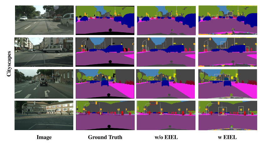
Figure 4: Comparison of the performance on Semantic Segmentation task. The pictures above from left to right are ground truth, label, baseline HRNet-W48-OCR without / with EIEL. Orange box indicate the better performance on pole, traffic sign and light, and the green ones are those with clearer pedestrians segmentation. Some obvious incorrect segmentation positions (w/o EIEL) in the third column are highlighted in red boxes.

Figure 4 shows semantic segmentation performance on cityscapes. In the forth column (with EIEL), the improved areas are framed in different colors. In the row 2 of right most column, the segmentation of the pedestrian legs is even better than what was provided in ground truth, because the man in the picture is wearing shorts with a gap between his legs.

We also achieve 82.9 mIoU on HRNet-OCR and 79.0 on BiSeNetV1 (78.86 originally) when using multi-scale inference (random scale on {0.25, 0.5, 0.75, 1.0, 1.25, 1.5, 1.75, 2.0}), which can outperform many other models.

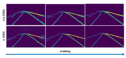
Figure 5: Performance comparison of the lane detection task (Tusimple). The picture from left to right is the training process until convergence is reached. EIEL corrected the wrong classification pixels, and the end of the lane is clearer.

4.2.2 Segmentation-based lane detection.

Figure 5 shows the training process with/without EIEL. The image and down-scaled ground truth have been showed in Figure.2. As our size of ground truth is $88*160$, the prediction boundaries are also grid-like. The first column is the model after 1st epoch, which are both disconnected on the left most lane and blurry on the right most lane, because they are occluded by cars. Adding EIEL fixes the wrong prediction and finally the lanes are all continuous after convergence. In addition, EIEL makes the prediction much straighter, sharper and precise on details than those without it.

It is noticed that in figure 6, our approach can let the shape at the end of the driveway clearer, and improve the mis-classification problem and lane blurry/missing situation. As marked in the pictures in the images, the far lane line in the first row of image is curved, and the blocked lane line in the third row of image is straight, and our inference accuracy is higher. The disconnection due to incorrect classification in the second row, and the missing lane lines due to occlusion in the fourth and fifth rows were also fixed. The experiments shows that EIEL can indeed improve the details segmentation, and have better inference ability in poor visual conditions.

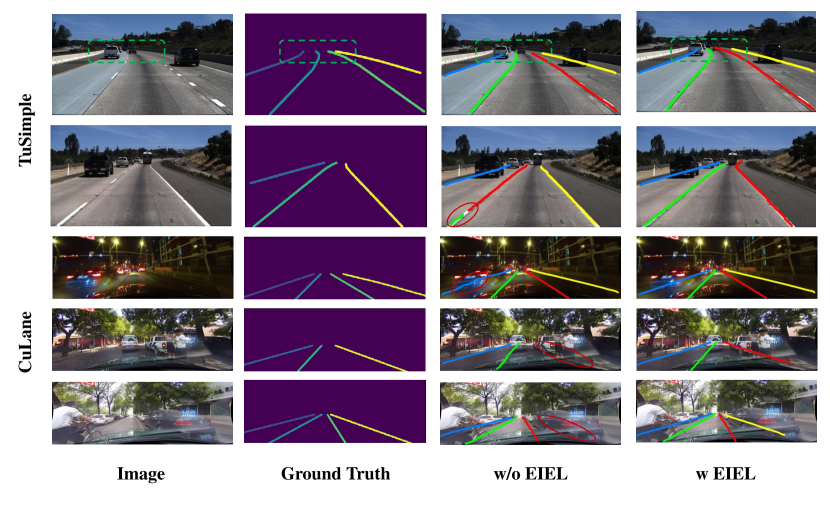
Figure 6: Performance on Lane Detection task with backbone ERFNet. From top to bottom, the baseline without EIEL are not curvy enough, line disconnected caused by wrong classify, bend as feature map blurry, lane missing caused by occlusion.

Model	train set	Acc (%)	FP	FN	Pix.F1
ENet	train	91.28	0.1899	0.1594	97.53
ENet+EIEL	train	94.00	0.1053	0.0919	97.82
ERFNet	train	91.14	0.1669	0.1494	97.34
ERFNet+EIEL	train	94.18	0.1131	0.0898	97.88

Table 2: Comparison of two baseline with / without EIEL on TuSimple. Set the batchsize to 4 and the training epoch w/o EIEL is around 40, while w EIEL within 30.

Method	Normal	Crowded	Dazzle	Shadow	No line	Arrow	Curve	Cross	Night	Total
ERFNet	85.60	67.14	59.40	60.72	44.07	78.99	60.79	1861	61.61	68.82
ERFNet+EIEL	88.96	71.29	62.66	72.69	47.26	84.14	60.55	2795	66.41	72.19
ERFNet+EIEL+IoU+LE	90.08	72.21	63.58	72.96	48.95	85.58	62.46	2201	68.50	73.76

Table 3: Comparison of class IoU and total IoU (threshold = 0.5) on baseline ERFNet with / without EIEL on CULane.

Table 2 and 3 shows the results on lane predictions of CULane and Tusimple, respectively. In experiment results of Tusimple, EIEL makes around 3% accuracy improvement, and significant reduces the FPR and FNR, showed in table 2. In CULane results, most of the categories IoU increase with the assistance of elastic energy loss as displayed in first two rows. Last row in table 3 is the results when adding two auxiliary loss functions $L_{IoU}$ and $L_{exist}$, where the former one guides the network to increase the pixel interaction of union, and the latter one is achieved by add an auxiliary branch of lane existence (LE), and calculated by binary cross entropy. These results show that the use of EIEL can significantly improve lane segmentation results and is suitable for any task requiring to obtain lane heat maps/probability maps. There are many other ways to tune the parameters, including setting the tusimple labels (5 lanes from left to fight, or 4 / 6 lanes on two sides of ego lane), batch size, learning rates, adding various auxiliary branches, etc. We do not focus too much on these improvement measures, but just make comparison on segmentation quality via experiments on the same code and machine until convergence.

Figure 7 shows some curves of the experimental process. The left column are validation losses, and the right column are average pixel accuracy and F1 measure. (a) and (b) are the experimental diagrams without EIEL, and (c) and (d) are the experimental diagrams with EIEL. Our method achieves early convergence (from about epoch 10), while the baseline curve oscillations do not flatten out until epoch 20. Due to the long-distance nature of our loss, the model EIEGSeg, is insensitive to the initial distribution and has the characteristics of training stability and rapid convergence.

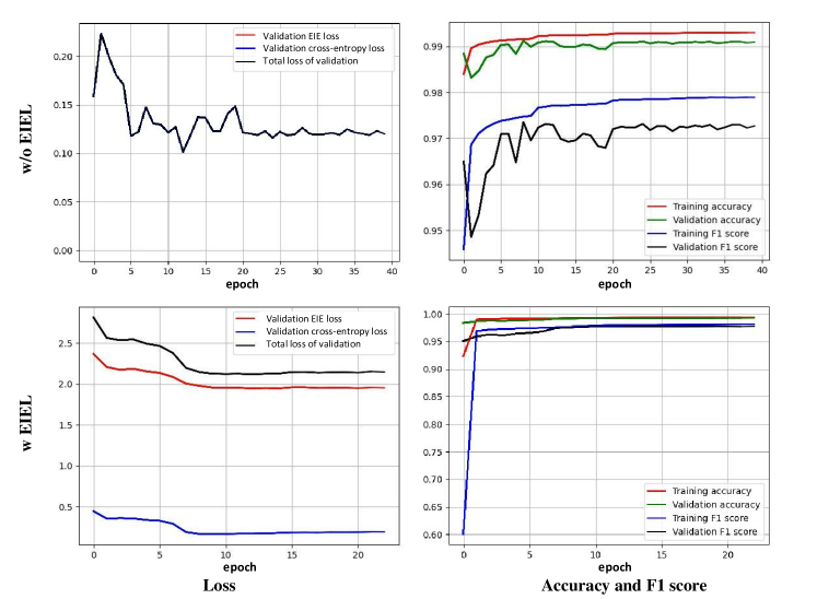
Figure 7: Illustration on how EIEL jointly trained with CE effects the loss value and pixel accuracy.

5 Conclusion

We proposed an EIEGSeg training strategy for multi class segmentation task in autonomous driving. It is proved to be robust on segmentation of geometry complex objects such as long-thin objects and small, irregular shaped objects. It can also be easily combined into different network architectures, especially the light-wight backbones, which can help achieve real-time inference in autonomous driving.

References

- [1] Eduardo Romera, José M Alvarez, Luis M Bergasa, and Roberto Arroyo. Erfnet: Efficient residual factorized convnet for real-time semantic segmentation. IEEE Transactions on Intelligent Transportation Systems, 19(1):263–272, 2017.
- [2] Jonathan Long, Evan Shelhamer, and Trevor Darrell. Fully convolutional networks for semantic segmentation. In Proceedings of the IEEE conference on computer vision and pattern recognition, pages 3431–3440, 2015.
- [3] Zongwei Zhou, Md Mahfuzur Rahman Siddiquee, Nima Tajbakhsh, and Jianming Liang. Unet++: Redesigning skip connections to exploit multiscale features in image segmentation. IEEE transactions on medical imaging, 39(6):1856–1867, 2019.
- [4] Adam Paszke, Abhishek Chaurasia, Sangpil Kim, and Eugenio Culurciello. Enet: A deep neural network architecture for real-time semantic segmentation. arXiv preprint arXiv:1606.02147, 2016.
- [5] Changqian Yu, Jingbo Wang, Chao Peng, Changxin Gao, Gang Yu, and Nong Sang. Bisenet: Bilateral segmentation network for real-time semantic segmentation. In Proceedings of the European conference on computer vision (ECCV), pages 325–341, 2018.
- [6] Changqian Yu, Changxin Gao, Jingbo Wang, Gang Yu, Chunhua Shen, and Nong Sang. Bisenet v2: Bilateral network with guided aggregation for real-time semantic segmentation. International Journal of Computer Vision, 129:3051–3068, 2021.
- [7] Xingang Pan, Jianping Shi, Ping Luo, Xiaogang Wang, and Xiaoou Tang. Spatial as deep: Spatial cnn for traffic scene understanding. In Proceedings of the AAAI Conference on Artificial Intelligence, volume 32, 2018.
- [8] Salih Can Yurtkulu, Yusuf Hüseyin Şahin, and Gozde Unal. Semantic segmentation with extended deeplabv3 architecture. In 2019 27th Signal Processing and Communications Applications Conference (SIU), pages 1–4. IEEE, 2019.
- [9] Jingchun Zhou, Mingliang Hao, Dehuan Zhang, Peiyu Zou, and Weishi Zhang. Fusion pspnet image segmentation based method for multi-focus image fusion. IEEE Photonics Journal, 11(6):1–12, 2019.
- [10] Seonkyeong Seong and Jaewan Choi. Semantic segmentation of urban buildings using a high-resolution network (hrnet) with channel and spatial attention gates. Remote Sensing, 13(16):3087, 2021.
- [11] Andrew Blake, Pushmeet Kohli, and Carsten Rother. Markov random fields for vision and image processing. MIT press, 2011.
- [12] John Lafferty, Andrew McCallum, and Fernando CN Pereira. Conditional random fields: Probabilistic models for segmenting and labeling sequence data. 2001.
- [13] Yuhui Yuan, Jingyi Xie, Xilin Chen, and Jingdong Wang. Segfix: Model-agnostic boundary refinement for segmentation. In Computer Vision–ECCV 2020: 16th European Conference, Glasgow, UK, August 23–28, 2020, Proceedings, Part XII 16, pages 489–506. Springer, 2020.
- [14] Tsung-Wei Ke, Jyh-Jing Hwang, Ziwei Liu, and Stella X Yu. Adaptive affinity fields for semantic segmentation. In Proceedings of the European conference on computer vision (ECCV), pages 587–602, 2018.
- [15] Henghui Ding, Xudong Jiang, Ai Qun Liu, Nadia Magnenat Thalmann, and Gang Wang. Boundary-aware feature propagation for scene segmentation. In Proceedings of the IEEE/CVF International Conference on Computer Vision, pages 6819–6829, 2019.
- [16] Shubhankar Borse, Ying Wang, Yizhe Zhang, and Fatih Porikli. Inverseform: A loss function for structured boundary-aware segmentation. In Proceedings of the IEEE/CVF conference on computer vision and pattern recognition, pages 5901–5911, 2021.
- [17] Chi Wang, Yunke Zhang, Miaomiao Cui, Peiran Ren, Yin Yang, Xuansong Xie, Xian-Sheng Hua, Hujun Bao, and Weiwei Xu. Active boundary loss for semantic segmentation. In Proceedings of the AAAI Conference on Artificial Intelligence, volume 36, pages 2397–2405, 2022.
- [18] Hoel Kervadec, Jihene Bouchtiba, Christian Desrosiers, Eric Granger, Jose Dolz, and Ismail Ben Ayed. Boundary loss for highly unbalanced segmentation. In International conference on medical imaging with deep learning, pages 285–296. PMLR, 2019.
- [19] Maxim Berman, Amal Rannen Triki, and Matthew B Blaschko. The lovász-softmax loss: A tractable surrogate for the optimization of the intersection-over-union measure in neural networks. In Proceedings of the IEEE conference on computer vision and pattern recognition, pages 4413–4421, 2018.
- [20] Yuan Lan, Yang Xiang, and Luchan Zhang. An elastic interaction-based loss function for medical image segmentation. In Medical Image Computing and Computer Assisted Intervention–MICCAI 2020: 23rd International Conference, Lima, Peru, October 4–8, 2020, Proceedings, Part V 23, pages 755–764. Springer, 2020.
- [21] Yang Xiang, Albert CS Chung, and Jian Ye. An active contour model for image segmentation based on elastic interaction. Journal of computational physics, 219(1):455–476, 2006.
- [22] Xiaoling Hu, Fuxin Li, Dimitris Samaras, and Chao Chen. Topology-preserving deep image segmentation. Advances in neural information processing systems, 32, 2019.