11institutetext: Jiangsu Engineering Center of Network Monitoring, Nanjing University of Information Science and Technology, Nanjing 210044, P.R.China
School of Computer and Software, Nanjing University of Information Science and Technology, Nanjing 210044, P.R.China
Jiangsu Engineering Center of Network Monitoring, Nanjing University of Information Science and Technology, Nanjing 210044, P.R.China
Hong Kong Applied Science and Technology Research Institute(ASTRI),Hong Kong 999077, China
School of Software, Qufu Normal University,Shandong 273165, China

Quantum-based Feature Selection for Multi-Classification Problem in Complex Systems with Edge Computing

Wenjie Liu 11    Junxiu Chen 22    Yuxiang Wang 33    Peipei Gao 44    Zhibin Lei 55    Xu Ma 66112233445566
Abstract

The complex systems with edge computing require a huge amount of multi-feature data to extract appropriate insights for their decision-making, so it is important to find a feasible feature selection method to improve the computational efficiency and save the resource consumption. In this paper, a quantum-based feature selection algorithm for the multi-classification problem, namely QReliefF, is proposed, which can effectively reduce the complexity of algorithm and improve its computational efficiency. First, all features of each sample are encoded into a quantum state by performing operations CMP𝐶𝑀𝑃CMP and Rysubscript𝑅𝑦R_{y}, then the amplitude estimation is applied to calculate the similarity between any two quantum states (i.e., two samples). According to the similarities, the Grover-Long method is utilized to find the nearest k𝑘k neighbor samples, and then the weight vector is updated. After a certain number of iterations through the above process, the desired features can be selected with regards to the final weight vector and the threshold τ𝜏\tau. Compared with the classical ReliefF algorithm, our algorithm reduces the complexity of similarity calculation from O(MN)𝑂𝑀𝑁O(MN) to O(M)𝑂𝑀O(M), the complexity of finding the nearest neighbor from O(M)𝑂𝑀O(M) to O(M)𝑂𝑀O(\sqrt{M}), and resource consumption from O(MN)𝑂𝑀𝑁O(MN) to O(MlogN)𝑂𝑀𝑙𝑜𝑔𝑁O(MlogN). Meanwhile, compared with the quantum Relief algorithm, our algorithm is superior in finding the nearest neighbor, reducing the complexity from O(M)𝑂𝑀O(M) to O(M)𝑂𝑀O(\sqrt{M}). Finally, in order to verify the feasibility of our algorithm, a simulation experiment based on Rigetti with a simple example is performed.

Keywords:
Q

uantum ReliefF algorithm, Edge computing, Complex systems, Feature selection, Amplitude estimation, Grover-Long method, Rigetti

1 Introduction

Complex systems [1] are nonlinear systems composed of agents that can act with local environmental information, which require big data to extract appropriate insights for their decision-making. In the cloud computing [2][3][4][5], the data transmission delay between the data sources and the cloud centers is problematic for many complex systems where responses are usually required to be time critical or real-time. Instead, a recently emerging computation paradigm, edge computing [6][7][8][9], is promising to cater for these requirements, as edge computing resources are deployed data sources which support time critical or real-time data processing and analysis. As we all know, the computing resources and storage resources of most intelligent terminals are very limited, which places higher requirements on the computing performance of algorithms, especially machine learning algorithms, in complex systems with edge computing.

Machine learning [10][11] continuously improves its performance through “experience”, where experience generally originates from massive data. At present, many machine learning algorithms based on massive data [12][13][14] have been proposed. In the practical scenario, the amount of data available for training is getting larger and larger, while the characteristics of data are becoming more and more abundant. Those data with redundant or unrelated features will cause the problem of “curse of dimensionality” [15], which greatly increases the computational complexity of the algorithm. One of the possible solutions is the dimension reduction [16], and the other is the feature selection [17].

Relief algorithm [18] is a well-known feature selection algorithm for the two-classification problem. It is widely used because of its excellent classification effect. However, the limitation of this algorithm is that it can only perform the binary classification, and the efficiency of the algorithm will be greatly affected when the data size and feature size increase. To extend the application of the algorithm, Kononenko [19] proposed a new feature selection algorithm for the multi-classification problem, namely ReliefF algorithm. It has the advantages of simple principle, convenient implementation and good results, and has been widely applied in various fields [20][21][22].

On the other hand, since Benioff [23] and Feynman [24] explored the theoretical possibilities of quantum computing, some excellent results have been proposed one after another. For instance, Shor’s algorithm [25] solves the problem of integer factorization in polynomial time. Grover’s algorithm [26] has a quadratic speedup to the problem of conducting a search through some unstructured database. These excellent results have prompted people to think about how to apply this computing power into machine learning algorithms. And thus a new research hotspot, quantum machine learning [27][28][29][30][31][32], has gradually formed. Although quantum technology provides a certain improvement in storage and computing power, the “curse of dimensionality” problem still exists in quantum machine learning. Therefore, the quantum-based dimensionality reduction method still has important research value. In 2018, Liu et al.[33] proposed a quantum Relief algorithm (namely QRelief algorithm) for the two-classification problem, which reduces the complexity of similarity calculation from O(MN)𝑂𝑀𝑁O(MN) to O(M)𝑂𝑀O(M).

As we know, in the application scenario of edge computing, there are various multi-classification problems based on distributed, massive and large-feature data. The objective of this study is to design a feasible feature selection method which can effectively get rid of redundant or unrelated features in machine learning, reducing the computation load of intelligent terminals, and thus meet the requirement of real-time data processing and analysis in edge computing. In this paper, we introduce some quantum technologies (such as CMP operation, amplitude estimation and Grover-Long method), and propose a quantum-based feature selection algorithm, namely QReliefF algorithm, for the multi-classification problem.

The main contributions of our work are:

(1) A quantum method is proposed to solve the problem of feature selection for the multi-classification problem in complex systems with edge computing. The proposed method fully demonstrates the quantum parallel processing capabilities that classical computing cannot match, and significantly reduces the computational complexity of the algorithm.

(2) The problem of finding nearest neighbor samples is firstly transformed into the similarity calculation of two quantum states (i.e., calculating their inner product) in quantum computing, and the Grover-long method is utilized to speed up the search of the targets.

(3) A simulation experiment based on Rigetti is performed to verify the feasibility of our algorithm.

The outline of this paper is as follows: The classic ReliefF algorithm is briefly reviewed in Sect. 2, and the proposed quantum ReliefF algorithm is proposed in detail in Sect. 3. Then, we illustrate the process of the algorithm with a simple example in Sect. 4, and perform the simulation experiment on Rigetti in Sect. 5. Subsequently, the efficiency of the algorithm is analyzed in Sect. 6, and the brief conclusion and discussion are summarized in the last section.

2 Review of ReliefF algorithm

ReliefF algorithm [19] is a feature selection algorithm which is used to handle the multi-classification problem. Before introducing our proposed quantum algorithm, let us review the detailed process of the algorithm.

Without loss of generality, suppose there are M𝑀M samples with N𝑁N features, and they can be divided into P𝑃P classes:

Cp={vq|vqN,q=1,2,,Mp},p{1,2,,P},formulae-sequencesubscript𝐶𝑝conditional-setsubscript𝑣𝑞formulae-sequencesubscript𝑣𝑞superscript𝑁𝑞12subscript𝑀𝑝𝑝12𝑃{C_{p}}=\left\{{{v_{q}}\left|{{v_{q}}\in{\mathbb{R}^{N}},q=1,2,\ldots,{M_{p}}}\right.}\right\},p\in\left\{{1,2,\ldots,P}\right\}, (1)

where vqsubscript𝑣𝑞{v_{q}} is the q𝑞q-th N𝑁N-feature sample that belongs to Class Cpsubscript𝐶𝑝{C_{p}}, vq=(vq1,vq2,,vqN)Tsubscript𝑣𝑞superscriptsubscript𝑣𝑞1subscript𝑣𝑞2subscript𝑣𝑞𝑁𝑇{v_{q}}={\left({{v_{q1}},{v_{q2}},\ldots,{v_{qN}}}\right)^{T}}. And the weight vector of N𝑁N features WT=(wt1,wt2,,wtN)T𝑊𝑇superscript𝑤subscript𝑡1𝑤subscript𝑡2𝑤subscript𝑡𝑁𝑇WT={(w{t_{1}},w{t_{2}},\cdots,w{t_{N}})^{T}} is initialized to all zeros, the upper limit of iteration is T𝑇T, and the relevance threshold (that differentiate the relevant and irrelevant features) is τ𝜏\tau (0τ10𝜏1{\rm{0}}\leq\tau\leq 1). The main steps of ReliefF algorithm are as follows (its pseudo code can be seen in Algorithm 1).

1 Init WT=(0,,0)T𝑊𝑇superscript00𝑇WT={(0,\cdots,0)^{T}}
2for t=1𝑡1t=1 to T𝑇T do
3     
4     Pick a sample u𝑢u randomly
5     Find k𝑘k nearest neighbor samples Hjsubscript𝐻𝑗{H_{j}} from the same class of sample u𝑢u.
6     for Cpclass(u)subscript𝐶𝑝𝑐𝑙𝑎𝑠𝑠𝑢{C_{p}}\neq class(u) do
7           Find k𝑘k nearest neighbor samples Mj(Cp)subscript𝑀𝑗subscript𝐶𝑝{M_{j}}(C_{p}) from the different Class Cpsubscript𝐶𝑝C_{p}
8           end for
9          for i=1𝑖1i=1 to N𝑁N do
10                WT[i]=WT[i]j=1kdiff(i,u,Hj)+Cpclass(u)[p(Cp)1p(class(u))j=1kdiff(i,u,Mj(Cp))]𝑊𝑇delimited-[]𝑖𝑊𝑇delimited-[]𝑖superscriptsubscript𝑗1𝑘𝑑𝑖𝑓𝑓𝑖𝑢subscript𝐻𝑗subscriptsubscript𝐶𝑝𝑐𝑙𝑎𝑠𝑠𝑢delimited-[]𝑝subscript𝐶𝑝1𝑝𝑐𝑙𝑎𝑠𝑠𝑢superscriptsubscript𝑗1𝑘𝑑𝑖𝑓𝑓𝑖𝑢subscript𝑀𝑗subscript𝐶𝑝WT\left[i\right]=WT\left[i\right]-\sum\limits_{j=1}^{k}{diff(i,u,{H_{j}})}{\kern 1.0pt}{\kern 1.0pt}{\kern 1.0pt}+\sum\limits_{{C_{p}}\notin class(u)}{[{{p(C_{p})}\over{1-p(class(u))}}\sum\limits_{j=1}^{k}{diff(i,u,{M_{j}}(C_{p}))}]}
11                end for
12               
13                end for
Select the most relevant features according to WT𝑊𝑇WT and τ𝜏\tau
Algorithm 1 ReliefF algorithm

At each iteration, ReliefF randomly selects a sample u𝑢u, and then searches for k𝑘k nearest neighbor samples by cosine distance from each class. The closest same-class sample is called Hjsubscript𝐻𝑗{H_{j}}, and the closest different-class sample is called Mj(Cp)subscript𝑀𝑗subscript𝐶𝑝{M_{j}}(C_{p}), where j={1,2,,k}𝑗12𝑘j=\{1,2,\cdots,k\}. The updating weight vector formula is shown as follows,

WT[i]=WT[i]j=1kdiff(i,u,Hj)+Cpclass(u)[p(Cp)1p(class(u))j=1kdiff(i,u,Mj(Cp))],𝑊𝑇delimited-[]𝑖𝑊𝑇delimited-[]𝑖superscriptsubscript𝑗1𝑘𝑑𝑖𝑓𝑓𝑖𝑢subscript𝐻𝑗subscriptsubscript𝐶𝑝𝑐𝑙𝑎𝑠𝑠𝑢delimited-[]𝑝subscript𝐶𝑝1𝑝𝑐𝑙𝑎𝑠𝑠𝑢superscriptsubscript𝑗1𝑘𝑑𝑖𝑓𝑓𝑖𝑢subscript𝑀𝑗subscript𝐶𝑝\begin{gathered}WT\left[i\right]=WT\left[i\right]-\sum\limits_{j=1}^{k}{diff(i,u,{H_{j}})}\hfill\\ +\sum\limits_{{C_{p}}\notin class(u)}{[\frac{{p(C_{p})}}{{1-p(class(u))}}\sum\limits_{j=1}^{k}{diff(i,u,{M_{j}}(C_{p}))}]}\hfill\\ \end{gathered}, (2)

where p(Cp)𝑝subscript𝐶𝑝p(C_{p}) represents the probability of randomly extracting samples of Class Cpsubscript𝐶𝑝C_{p}, and the definition of diff(i,u,v)𝑑𝑖𝑓𝑓𝑖𝑢𝑣diff(i,u,v) function is as follows,

diff(i,u,v)={|u[i]v[i]|max(i)min(i)iiscontinuous0ui=vi1uivi.𝑑𝑖𝑓𝑓𝑖𝑢𝑣cases𝑢delimited-[]𝑖𝑣delimited-[]𝑖𝑖𝑖𝑖𝑖𝑠𝑐𝑜𝑛𝑡𝑖𝑛𝑢𝑜𝑢𝑠missing-subexpressionmissing-subexpression0subscript𝑢𝑖subscript𝑣𝑖missing-subexpressionmissing-subexpression1subscript𝑢𝑖subscript𝑣𝑖missing-subexpressionmissing-subexpressiondiff(i,u,v)=\left\{\begin{array}[]{lcl}{{{\left|{u[i]-v[i]}\right|}\over{\max(i)-\min(i)}}}{\kern 4.0pt}i{\kern 2.0pt}is{\kern 2.0pt}continuous\\ 0{\kern 28.0pt}{u_{i}}={v_{i}}\\ 1{\kern 30.0pt}{u_{i}}\neq{v_{i}}\end{array}.\right. (3)

After iterating T𝑇T times, the final weight vector is obtained. Through the relevance threshold τ𝜏\tau, we can retain relevant features and discard irrelevant features.

ReliefF algorithm is an extension of Relief algorithm that extends the two-classification problem to multi-classification scenario. However, with the increase of category size, sample size and sample features, ReliefF algorithm will also face with the problem of “dimension disaster”, and the speed of the algorithm will also drop sharply. So, how to improve the efficiency of ReliefF algorithm becomes an urgent problem to be solved.

3 The proposed QReliefF algorithm

In order to implement the feature selection for the multi-classification problem in complex systems with edge computing, a feasible quantum ReliefF algorithm is introduced in this section. Suppose the sample sets Cp={vq=(vq1,vq2,,vqN)T|vqN,q=1,2,,Mp}subscript𝐶𝑝conditional-setsubscript𝑣𝑞superscriptsubscript𝑣𝑞1subscript𝑣𝑞2subscript𝑣𝑞𝑁𝑇formulae-sequencesubscript𝑣𝑞superscript𝑁𝑞12subscript𝑀𝑝{{C}_{p}}=\left\{{{v_{q}}={\left({{v_{q1}},{v_{q2}},\ldots,{v_{qN}}}\right)^{T}}\left|{{{v}_{q}}\in{\mathbb{R}^{N}},q=1,2,\ldots,{M_{p}}}\right.}\right\} (p𝑝p represents the category of classification, p{1,2,,P}𝑝12𝑃p\in\left\{{1,2,\ldots,P}\right\}), the weight vector WT𝑊𝑇WT, the upper limit T𝑇T, and the relevance threshold τ𝜏\tau are the same as classical ReliefF algorithm defined in Sect. II. Different from the classical one, all the features of each sample are represented as a quantum superposition state, thus the problem of finding nearest neighbor samples is transformed into the similarity calculation of two quantum states (i.e., calculating their inner product). And the similarity between any two samples can be calculated in parallel in the way of quantum mechanics. Algorithm 2 describes the process of our algorithm in detail, and the specific steps are as bellow.

1 Init WT=(0,,0)T𝑊𝑇superscript00𝑇WT={(0,\cdots,0)^{T}}
2Normalized the sample sets: CpC¯psubscript𝐶𝑝subscript¯𝐶𝑝{C_{p}}\to{{\bar{C}}_{p}}
3prepare quantum states for all samples by operations CMP𝐶𝑀𝑃CMP and Rysubscript𝑅𝑦R_{y}, respectively. |ϕpq=1N|qi=0N1|i|1(1|v¯qi|2|0+v¯qi|1)subscriptketsubscriptitalic-ϕ𝑝𝑞1𝑁ket𝑞superscriptsubscript𝑖0𝑁1ket𝑖ket11superscriptsubscript¯𝑣𝑞𝑖2ket0subscript¯𝑣𝑞𝑖ket1{\left|{{\phi_{p}}}\right\rangle_{q}}={1\over{\sqrt{N}}}\left|q\right\rangle\sum\limits_{i=0}^{N-1}{\left|i\right\rangle\left|1\right\rangle\left({\sqrt{1-{{\left|{{\bar{v}_{q{\kern 1.0pt}i}}}\right|}^{2}}}\left|0\right\rangle+{\bar{v}_{q{\kern 1.0pt}i}}\left|1\right\rangle}\right)}
4for t=1𝑡1t=1 to T𝑇T do
5     
6     Select a state |ϕketitalic-ϕ\left|\phi\right\rangle from {|ϕpq}subscriptketsubscriptitalic-ϕ𝑝𝑞\left\{{{{\left|{{\phi_{p}}}\right\rangle}_{q}}}\right\} randomly which corresponds to u𝑢u
7     Perform swap operation on |ϕketitalic-ϕ\left|\phi\right\rangle and obtain |φ=1N|li=0N1|i(1|u¯i|2|0+u¯i|1)|1ket𝜑1𝑁ket𝑙superscriptsubscript𝑖0𝑁1ket𝑖1superscriptsubscript¯𝑢𝑖2ket0subscript¯𝑢𝑖ket1ket1\left|\varphi\right\rangle={1\over{\sqrt{N}}}\left|l\right\rangle\sum\limits_{i=0}^{N-1}{\left|i\right\rangle\left({\sqrt{1-{{\left|{{\bar{u}_{i}}}\right|}^{2}}}\left|0\right\rangle+{\bar{u}_{i}}\left|1\right\rangle}\right)}\left|1\right\rangle
8     The similarity information coded into quantum state |βp=1Mpq=1Mp|q|v¯qu¯subscriptket𝛽𝑝1subscript𝑀𝑝superscriptsubscript𝑞1subscript𝑀𝑝ket𝑞ketsubscript¯𝑣𝑞¯𝑢{\left|\beta\right\rangle_{p}}={1\over{\sqrt{{M_{p}}}}}\sum\limits_{q=1}^{{M_{p}}}{\left|q\right\rangle}\left|{{\bar{v}_{q}}-\bar{u}}\right\rangle through swaptest𝑠𝑤𝑎𝑝𝑡𝑒𝑠𝑡swap{\kern 1.0pt}{\kern 1.0pt}{\kern 1.0pt}{\kern 1.0pt}test, the inner product and amplitude estimation operations
9     The nearest k𝑘k samples in each class are obtained by Grover-Long method
10     for i=1𝑖1i=1 to N𝑁N do
11           WT[i]=WT[i]j=1kdiff(i,u¯,Hj)+C¯pclass(u¯)[p(C¯p)1p(class(u¯))j=1kdiff(i,u¯,Mj(C¯p))]𝑊𝑇delimited-[]𝑖𝑊𝑇delimited-[]𝑖superscriptsubscript𝑗1𝑘𝑑𝑖𝑓𝑓𝑖¯𝑢subscript𝐻𝑗subscriptsubscript¯𝐶𝑝𝑐𝑙𝑎𝑠𝑠¯𝑢delimited-[]𝑝subscript¯𝐶𝑝1𝑝𝑐𝑙𝑎𝑠𝑠¯𝑢superscriptsubscript𝑗1𝑘𝑑𝑖𝑓𝑓𝑖¯𝑢subscript𝑀𝑗subscript¯𝐶𝑝WT\left[i\right]=WT\left[i\right]-\sum\limits_{j=1}^{k}{diff(i,\bar{u},{H_{j}})}+\sum\limits_{{\bar{C}_{p}}\notin class(\bar{u})}{[{{p(\bar{C}_{p})}\over{1-p(class(\bar{u}))}}\sum\limits_{j=1}^{k}{diff(i,\bar{u},{M_{j}}(\bar{C}_{p}))}]}
12           end for
13          
14           end for
15          WT¯=(1/T)WT¯𝑊𝑇1/𝑇𝑊𝑇\overline{WT}=\left({{1\mathord{\left/{\vphantom{1T}}\right.\kern-1.2pt}T}}\right)WT
16          for i=1𝑖1i=1 to N𝑁N do
17               
18               if (WTi¯τ)¯𝑊subscript𝑇𝑖𝜏\left({\overline{W{T_{i}}}\geq\tau}\right) then
19                     The i-th feature is relevant;
20                    
21                     else
22                          The i-th feature is not relevant;
23                         
24                          end if
25                         
26                          end for
Algorithm 2 Quantum ReliefF algorithm

3.1 State preparation

In order to store classical information in quantum states, we need to normalize the sample sets:

CpC¯p={v¯q=(v¯q1,v¯q2,,v¯qN)T},subscript𝐶𝑝subscript¯𝐶𝑝subscript¯𝑣𝑞superscriptsubscript¯𝑣𝑞1subscript¯𝑣𝑞2subscript¯𝑣𝑞𝑁𝑇{C_{p}}\to{{\bar{C}}_{p}}=\left\{{{\bar{v}_{q}}={\left({{\bar{v}_{q1}},{\bar{v}_{q2}},\ldots,{\bar{v}_{qN}}}\right)^{T}}}\right\}, (4)

where

v¯qi=vqii=1N|vqi|2,i=1,2,,N.formulae-sequencesubscript¯𝑣𝑞𝑖subscript𝑣𝑞𝑖superscriptsubscript𝑖1𝑁superscriptsubscript𝑣𝑞𝑖2𝑖12𝑁{\bar{v}_{qi}}={{{v_{qi}}}\over{\sqrt{\sum\limits_{i=1}^{N}{{{\left|{{v_{qi}}}\right|}^{2}}}}}},i=1,2,\ldots,N. (5)

Obviously, v¯qisubscript¯𝑣𝑞𝑖{{\bar{v}}_{qi}} is a real number, and v¯qi(0,1)subscript¯𝑣𝑞𝑖01{{\bar{v}}_{qi}}\in\left({0,1}\right). Then we prepare the initial quantum states as below,

|ϕpq=1N|qi=0N1|i|1(1|v¯qi|2|0+v¯qi|1),subscriptketsubscriptitalic-ϕ𝑝𝑞1𝑁ket𝑞superscriptsubscript𝑖0𝑁1ket𝑖ket11superscriptsubscript¯𝑣𝑞𝑖2ket0subscript¯𝑣𝑞𝑖ket1{\left|{{\phi_{p}}}\right\rangle_{q}}=\frac{1}{{\sqrt{N}}}\left|q\right\rangle\sum\limits_{i=0}^{N-1}{\left|i\right\rangle\left|1\right\rangle\left({\sqrt{1-{{\left|{{\bar{v}_{q{\kern 1.0pt}i}}}\right|}^{2}}}\left|0\right\rangle+{\bar{v}_{q{\kern 1.0pt}i}}\left|1\right\rangle}\right)}, (6)

where |ϕpqsubscriptketsubscriptitalic-ϕ𝑝𝑞{\left|{{\phi_{p}}}\right\rangle_{q}} corresponds to the quantum state of the q𝑞q-th sample that belongs to Class C¯psubscript¯𝐶𝑝{\bar{C}_{p}}, and v¯qisubscript¯𝑣𝑞𝑖{\bar{v}_{q{\kern 1.0pt}i}} represents the i𝑖i-th eigenvalue of the q𝑞q-th sample. Assume our initial state is |q|0n|1|0(n=log2(N))ket𝑞superscriptket0tensor-productabsent𝑛ket1ket0𝑛subscript2𝑁\left|q\right\rangle{\left|0\right\rangle^{\otimes n}}\left|1\right\rangle\left|0\right\rangle(n=\left\lceil{{{\log}_{2}}(N)}\right\rceil), the construction scheme of the quantum state |ϕpqsubscriptketsubscriptitalic-ϕ𝑝𝑞{\left|{{\phi_{p}}}\right\rangle_{q}} includes the following steps.

First, we perform Hadamard and CMP operations for |0nsuperscriptket0tensor-productabsent𝑛{\left|0\right\rangle^{\otimes n}} and get a new state:

|0nHandCMPoperations1Ni=0N1|i,H𝑎𝑛𝑑CMP𝑜𝑝𝑒𝑟𝑎𝑡𝑖𝑜𝑛𝑠superscriptket0tensor-productabsent𝑛1𝑁superscriptsubscript𝑖0𝑁1ket𝑖{\left|0\right\rangle^{\otimes n}}\xrightarrow{\emph{H}{\kern 2.0pt}and{\kern 2.0pt}\emph{CMP}{\kern 2.0pt}operations}{{\rm{1}}\over{\sqrt{N}}}\sum\limits_{i=0}^{N-1}{\left|i\right\rangle}, (7)

and its circuit diagram is shown in Fig. 1, where the definition of CMP operation is

CMP|i|N|0={|i|N|0,i<N|i|N|1,iN.𝐶𝑀𝑃ket𝑖ket𝑁ket0casesket𝑖ket𝑁ket0𝑖𝑁missing-subexpressionmissing-subexpressionmissing-subexpressionmissing-subexpressionmissing-subexpressionmissing-subexpressionmissing-subexpressionmissing-subexpressionmissing-subexpressionmissing-subexpressionmissing-subexpressionmissing-subexpressionmissing-subexpressionmissing-subexpressionmissing-subexpressionmissing-subexpressionmissing-subexpressionmissing-subexpressionmissing-subexpressionket𝑖ket𝑁ket1𝑖𝑁missing-subexpressionmissing-subexpressionmissing-subexpressionmissing-subexpressionmissing-subexpressionmissing-subexpressionmissing-subexpressionmissing-subexpressionmissing-subexpressionmissing-subexpressionmissing-subexpressionmissing-subexpressionmissing-subexpressionmissing-subexpressionmissing-subexpressionmissing-subexpressionmissing-subexpressionmissing-subexpressionmissing-subexpressionCMP\left|i\right\rangle\left|N\right\rangle\left|0\right\rangle=\left\{{\begin{array}[]{*{20}{c}}{\left|i\right\rangle\left|N\right\rangle\left|0\right\rangle,i<N}\\ {\left|i\right\rangle\left|N\right\rangle\left|1\right\rangle,i\geq N}\end{array}}.\right. (8)

The function of CMP operation is to cut the quantum state larger than N𝑁N, and its circuit diagram is shown in Fig. 2. |iket𝑖\left|i\right\rangle and |Nket𝑁\left|N\right\rangle represent a single qubit. The implementation of CMP operation needs to repeatedly implement such a circuit n𝑛n times. After measurement, if the lowest register is |1ket1\left|1\right\rangle, it means that i>N𝑖𝑁i>N.

Refer to caption

Figure 1: Quantum circuit of getting 1Ni=0N1|i1𝑁superscriptsubscript𝑖0𝑁1ket𝑖{{\rm{1}}\over{\sqrt{N}}}\sum\limits_{i=0}^{N-1}{\left|i\right\rangle}, and H is the Hadamard operation, \circ represents the control qubit conditional being set to zero.

Refer to caption

Figure 2: Quantum circuit of CMP operation, and \bullet represents the control qubit conditional being set to one.

Next, we perform the unitary rotation operation Rysubscript𝑅𝑦R_{y}:

Ry(2sin1v¯qi)=[1|v¯qi|2v¯qiv¯qi1|v¯qi|2],subscript𝑅𝑦2superscript1subscript¯𝑣𝑞𝑖delimited-[]1superscriptsubscript¯𝑣𝑞𝑖2subscript¯𝑣𝑞𝑖missing-subexpressionmissing-subexpressionmissing-subexpressionmissing-subexpressionmissing-subexpressionmissing-subexpressionmissing-subexpressionmissing-subexpressionmissing-subexpressionmissing-subexpressionmissing-subexpressionmissing-subexpressionmissing-subexpressionmissing-subexpressionmissing-subexpressionmissing-subexpressionmissing-subexpressionmissing-subexpressionsubscript¯𝑣𝑞𝑖1superscriptsubscript¯𝑣𝑞𝑖2missing-subexpressionmissing-subexpressionmissing-subexpressionmissing-subexpressionmissing-subexpressionmissing-subexpressionmissing-subexpressionmissing-subexpressionmissing-subexpressionmissing-subexpressionmissing-subexpressionmissing-subexpressionmissing-subexpressionmissing-subexpressionmissing-subexpressionmissing-subexpressionmissing-subexpressionmissing-subexpression{R_{y}}\left({2{{\sin}^{-1}}{\bar{v}_{qi}}}\right)=\left[{\begin{array}[]{*{20}{c}}{\sqrt{1-{{\left|{{\bar{v}_{qi}}}\right|}^{2}}}}&{-{\bar{v}_{qi}}}\\ {{\bar{v}_{qi}}}&{\sqrt{1-{{\left|{{\bar{v}_{qi}}}\right|}^{2}}}}\end{array}}\right], (9)

on the last qubit to obtain our target quantum state |ϕpqsubscriptketsubscriptitalic-ϕ𝑝𝑞{\left|{{\phi_{p}}}\right\rangle_{q}},

1N|qi=0N1|i|1(1|v¯qi|2|0+v¯qi|1).1𝑁ket𝑞superscriptsubscript𝑖0𝑁1ket𝑖ket11superscriptsubscript¯𝑣𝑞𝑖2ket0subscript¯𝑣𝑞𝑖ket1\frac{1}{{\sqrt{N}}}\left|q\right\rangle\sum\limits_{i=0}^{N-1}{\left|i\right\rangle\left|1\right\rangle\left({\sqrt{1-{{\left|{{\bar{v}_{q{\kern 1.0pt}i}}}\right|}^{2}}}\left|0\right\rangle+{\bar{v}_{q{\kern 1.0pt}i}}\left|1\right\rangle}\right)}. (10)

3.2 Similarity calculation

After the state preparation, the information of the samples is encoded into the quantum superposition state {|ϕpq}subscriptketsubscriptitalic-ϕ𝑝𝑞\left\{{{{\left|{{\phi_{p}}}\right\rangle}_{q}}}\right\}. In this paper, we use the cosine distance to define the similarity between the random sample u¯¯𝑢\bar{u} and other sample (e.g., v¯qsubscript¯𝑣𝑞\bar{v}_{q}),

s(u¯,v¯q)=.|cosθ|2=|u¯|v¯q|2|u¯|2|v¯q|2.superscript.𝑠¯𝑢subscript¯𝑣𝑞superscript𝜃2superscriptdelimited-⟨⟩|¯𝑢subscript¯𝑣𝑞2superscript¯𝑢2superscriptsubscript¯𝑣𝑞2s\left({\bar{u},{\bar{v}_{q}}}\right)\buildrel\textstyle.\over{=}{\left|{\cos\theta}\right|^{2}}={{{{\left|{\left\langle{\bar{u}}\mathrel{\left|{\vphantom{\bar{u}{{\bar{v}_{q}}}}}\right.\kern-1.2pt}{{{\bar{v}_{q}}}}\right\rangle}\right|}^{2}}}\over{{{\left|\bar{u}\right|}^{2}}\cdot{{\left|{{\bar{v}_{q}}}\right|}^{2}}}}. (11)

Referring to Eqs. (4) and (5), |u¯|2superscript¯𝑢2{\left|{\bar{u}}\right|^{2}} and |v¯q|2superscriptsubscript¯𝑣𝑞2{\left|{{\bar{v}_{q}}}\right|^{2}} are 1, Eq. 11 can be simplified as follows,

s(u¯,v¯q)=|u¯|v¯q|2.𝑠¯𝑢subscript¯𝑣𝑞superscriptdelimited-⟨⟩|¯𝑢subscript¯𝑣𝑞2s(\bar{u},{\bar{v}_{q}})={\left|{\left\langle{\bar{u}}\mathrel{\left|{\vphantom{\bar{u}{{\bar{v}_{q}}}}}\right.\kern-1.2pt}{{{\bar{v}_{q}}}}\right\rangle}\right|^{2}}. (12)

First, |ϕketitalic-ϕ\left|\phi\right\rangle (i.e., the sample u¯¯𝑢\bar{u}) is randomly selected from {|ϕpq}subscriptketsubscriptitalic-ϕ𝑝𝑞\left\{{{{\left|{{\phi_{p}}}\right\rangle}_{q}}}\right\} which is the l𝑙l-th sample in Class C¯psubscript¯𝐶𝑝{\bar{C}_{p}}, as shown in the following equation,

|ϕ=1N|li=0N1|i|1(1|u¯i|2|0+u¯i|1).ketitalic-ϕ1𝑁ket𝑙superscriptsubscript𝑖0𝑁1ket𝑖ket11superscriptsubscript¯𝑢𝑖2ket0subscript¯𝑢𝑖ket1\left|\phi\right\rangle=\frac{1}{{\sqrt{N}}}\left|l\right\rangle\sum\limits_{i=0}^{N-1}{\left|i\right\rangle\left|1\right\rangle\left({\sqrt{1-{{\left|{{\bar{u}_{i}}}\right|}^{2}}}\left|0\right\rangle+{\bar{u}_{i}}\left|1\right\rangle}\right)}. (13)

Then, a swap𝑠𝑤𝑎𝑝swap operation is performed on |ϕketitalic-ϕ\left|\phi\right\rangle to get

|φ=1N|li=0N1|i(1|u¯i|2|0+u¯i|1)|1.ket𝜑1𝑁ket𝑙superscriptsubscript𝑖0𝑁1ket𝑖1superscriptsubscript¯𝑢𝑖2ket0subscript¯𝑢𝑖ket1ket1\left|\varphi\right\rangle=\frac{1}{{\sqrt{N}}}\left|l\right\rangle\sum\limits_{i=0}^{N-1}{\left|{i}\right\rangle\left({\sqrt{1-{{\left|{{\bar{u}_{i}}}\right|}^{2}}}\left|0\right\rangle+{\bar{u}_{i}}\left|1\right\rangle}\right)\left|1\right\rangle}. (14)

Next, a swap test (its circuit is given in Fig.3) is performed on (|φ,|ϕpq)ket𝜑subscriptketsubscriptitalic-ϕ𝑝𝑞\left({\left|\varphi\right\rangle,{\kern 1.0pt}{\kern 1.0pt}{\kern 1.0pt}{\kern 1.0pt}{\kern 1.0pt}{\kern 1.0pt}{{\left|{{\phi_{p}}}\right\rangle}_{q}}}\right) and obtain

|ψ=12|0(|φ|ϕpq+|ϕpq|φ)+12|1(|φ|ϕpq|ϕpq|φ).ket𝜓12ket0ket𝜑subscriptketsubscriptitalic-ϕ𝑝𝑞subscriptketsubscriptitalic-ϕ𝑝𝑞ket𝜑12ket1ket𝜑subscriptketsubscriptitalic-ϕ𝑝𝑞subscriptketsubscriptitalic-ϕ𝑝𝑞ket𝜑\left|\psi\right\rangle={1\over 2}\left|0\right\rangle(\left|\varphi\right\rangle{\left|{{\phi_{p}}}\right\rangle_{q}}+{\left|{{\phi_{p}}}\right\rangle_{q}}\left|\varphi\right\rangle)+{1\over 2}\left|1\right\rangle(\left|\varphi\right\rangle{\left|{{\phi_{p}}}\right\rangle_{q}}-{\left|{{\phi_{p}}}\right\rangle_{q}}\left|\varphi\right\rangle). (15)
Figure 3: Quantum circuit of swap test operation, and the symbol of two crosses connected by a line represents the swap operation.

From Eq. (15), we know the probability of measurement result being |1ket1\left|1\right\rangle is

Pql(1)=ψ||11|II|ψ=[121|(φ|ϕp|qϕp|qφ|)]|11|II[121|(|φ|ϕpq|ϕpq|φ)]=1212|φ|ϕpq|2,\begin{gathered}P_{q}^{l}(1)=\left\langle\psi\right|\left|1\right\rangle\langle 1|\otimes I\otimes I\left|\psi\right\rangle\hfill\\ \;\;\;\;\;\;\;\;\;=\left[{{1\over 2}\left\langle 1\right|\left({\left\langle\varphi\right|{{\left\langle{{\phi_{p}}}\right|}_{q}}-{{\left\langle{{\phi_{p}}}\right|}_{q}}\left\langle\varphi\right|}\right)}\right]\left|1\right\rangle\langle 1|\otimes I\otimes I\hfill\\ \;\;\;\;\;\;\;\;\;\;\;\;\;\left[{{1\over 2}\langle 1|\left({\left|\varphi\right\rangle{{\left|{{\phi_{p}}}\right\rangle}_{q}}-{{\left|{{\phi_{p}}}\right\rangle}_{q}}\left|\varphi\right\rangle}\right)}\right]\hfill\\ \;\;\;\;\;\;\;\;\;={1\over 2}-{1\over 2}{\left|{{{\left\langle{\varphi\left|{{\phi_{p}}}\right.}\right\rangle}_{q}}}\right|^{2}},\hfill\\ \end{gathered} (16)

In addition, the inner product between |φket𝜑\left|\varphi\right\rangle and |ϕpqsubscriptketsubscriptitalic-ϕ𝑝𝑞{{\left|{{\phi_{p}}}\right\rangle}_{q}} (i.e., the prepared state) can be calculated as below,

φ|ϕpq=1Ni(u¯i)v¯qi=1Nu¯|v¯q.subscriptdelimited-⟨⟩|𝜑subscriptitalic-ϕ𝑝𝑞1𝑁subscript𝑖subscript¯𝑢𝑖subscript¯𝑣𝑞𝑖1𝑁delimited-⟨⟩|¯𝑢subscript¯𝑣𝑞{\left\langle{\varphi}\mathrel{\left|{\vphantom{\varphi{{\phi_{p}}}}}\right.\kern-1.2pt}{{{\phi_{p}}}}\right\rangle_{q}}={1\over N}\sum\limits_{i}{\left({{\bar{u}_{i}}}\right)*{\bar{v}_{qi}}}={1\over N}\left\langle{\bar{u}}\mathrel{\left|{\vphantom{\bar{u}{{\bar{v}_{q}}}}}\right.\kern-1.2pt}{{{\bar{v}_{q}}}}\right\rangle. (17)

Combining Eq. (16) with Eq. (17), we can get the similarity between samples u¯¯𝑢\bar{u} and v¯qsubscript¯𝑣𝑞\bar{v}_{q},

s(u¯,v¯q)=(12Pql(C¯p)(1))N2𝑠¯𝑢subscript¯𝑣𝑞12superscriptsubscript𝑃𝑞𝑙subscript¯𝐶𝑝1superscript𝑁2s(\bar{u},{\bar{v}_{q}})=\left({1-2P_{q}^{l\left({{\bar{C}_{p}}}\right)}(1)}\right){N^{2}} (18)

Since N𝑁N is a constant value and u¯|v¯qdelimited-⟨⟩|¯𝑢subscript¯𝑣𝑞\left\langle{\bar{u}}\mathrel{\left|{\vphantom{\bar{u}{{\bar{v}_{q}}}}}\right.\kern-1.2pt}{{{\bar{v}_{q}}}}\right\rangle is the angle cosine between the random sample u¯¯𝑢\bar{u} and other sample v¯qsubscript¯𝑣𝑞{\bar{v}_{q}} (e.g., in Class C¯psubscript¯𝐶𝑝{\bar{C}_{p}}), then the smaller s(u¯,v¯q)𝑠¯𝑢subscript¯𝑣𝑞s(\bar{u},{\bar{v}_{q}}) is, the smaller cosine distance is, which indicates that these two samples are more similar.

Then we can rewrite Eq. (15) as bellow:

|αp=1Mpq=1Mp|q(1s(u¯,v¯q)|0+s(u¯,v¯q)|1).subscriptket𝛼𝑝1subscript𝑀𝑝superscriptsubscript𝑞1subscript𝑀𝑝ket𝑞1𝑠¯𝑢subscript¯𝑣𝑞ket0𝑠¯𝑢subscript¯𝑣𝑞ket1{\left|\alpha\right\rangle_{p}}={1\over{\sqrt{{M_{p}}}}}\sum\limits_{q=1}^{{M_{p}}}{\left|q\right\rangle}\left({\sqrt{1-s(\bar{u},{\bar{v}_{q}})}\left|0\right\rangle+\sqrt{s(\bar{u},{\bar{v}_{q}})}\left|1\right\rangle}\right). (19)

3.3 Finding the nearest neighbor samples

[Uncaptioned image]

First, the quantum amplitude estimation method [34] is applied to store the similarity of the sample u¯¯𝑢\bar{u} and v¯qsubscript¯𝑣𝑞\bar{v}_{q} in the last qubit,

|βp=1Mpq=1Mp|q|s(u¯,v¯q),subscriptket𝛽𝑝1subscript𝑀𝑝superscriptsubscript𝑞1subscript𝑀𝑝ket𝑞ket𝑠¯𝑢subscript¯𝑣𝑞{\left|\beta\right\rangle_{p}}={1\over{\sqrt{{M_{p}}}}}\sum\limits_{q=1}^{{M_{p}}}{\left|q\right\rangle}\left|{s\left({\bar{u},{{\bar{v}}_{q}}}\right)}\right\rangle, (20)

where p{1,2,,P}𝑝12𝑃p\in\left\{{1,2,\ldots,P}\right\}, and its quantum circuit diagram is given in Fig. 4.

Refer to caption

Figure 4: Quantum circuit of amplitude estimation operation, GJsuperscript𝐺𝐽{G^{J}} represents J𝐽J iterations of Grover-Long method [35] and FM1superscriptsubscript𝐹𝑀1F_{M}^{-1} represents the inverse Fourier transform [36].

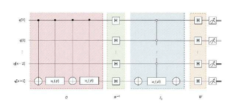
In the Grover-Long method [35], one iteration can be divided into four operations, i.e., G=WI0W1O𝐺𝑊subscript𝐼0superscript𝑊1𝑂G=-WI_{0}W^{-1}O, and its quantum circuit is shown in Fig. 5. O𝑂O is an oracle operation which performs a phase inversion on the targets:

O=eiϕ|vv|+τ=0,τv2n1|ττ|,𝑂superscript𝑒𝑖italic-ϕket𝑣quantum-operator-product𝑣superscriptsubscriptformulae-sequence𝜏0𝜏𝑣superscript2𝑛1𝜏bra𝜏O={e^{i\phi}}\left|v\right\rangle\left\langle v\right|+\sum\limits_{\tau=0,\tau\neq v}^{{2^{n}}-1}{\left|\tau\right\rangle\left\langle\tau\right|}, (21)

where v𝑣v is the position of eiϕsuperscript𝑒𝑖italic-ϕ{e^{i\phi}} in the diagonal matrix. The position v𝑣v of eiϕsuperscript𝑒𝑖italic-ϕ{e^{i\phi}} is divided into two cases. If v𝑣v is odd, the u1(ϕ)subscript𝑢1italic-ϕu_{1}(\phi) operation will be applied to the lowest qubit,

u1(ϕ)=diag[1,eiϕ].subscript𝑢1italic-ϕdiag1superscript𝑒𝑖italic-ϕu_{1}(\phi)=\operatorname{diag}\left[1,e^{i\phi}\right]. (22)

If v𝑣v is even, X,u1(ϕ),X𝑋subscript𝑢1italic-ϕ𝑋X,u_{1}(\phi),X operations will be applied to the lowest qubit.

Besides, I0subscript𝐼0I_{0} is a conditional phase shift operation which performs a phase inversion on |0ket0|0\rangle:

I0=eiϕ|00|+τ=12n1|ττ|=diag[eiϕ,1,,1]2n,subscript𝐼0superscript𝑒𝑖italic-ϕket0quantum-operator-product0superscriptsubscript𝜏1superscript2𝑛1𝜏bra𝜏diagsubscriptsuperscript𝑒𝑖italic-ϕ11superscript2𝑛{I_{0}}={e^{i\phi}}\left|0\right\rangle\left\langle 0\right|+\sum\limits_{\tau{\rm{=}}1}^{{2^{n}}-1}{\left|\tau\right\rangle\left\langle\tau\right|}={\mathop{\rm diag}\nolimits}{\left[{{e^{i\phi}},1,\ldots,1}\right]_{{2^{n}}}}, (23)
ϕ=2arcsin(sinπ4J+2sinη).italic-ϕ2𝜋4𝐽2𝜂\phi=2\arcsin\left(\frac{\sin\frac{\pi}{4J+2}}{\sin\eta}\right). (24)

where sinη=MN𝜂𝑀𝑁\sin\eta=\sqrt{\frac{M}{N}}, J𝐽J represents the number of iteration.

Refer to caption
Figure 5: Quantum circuit with one iteration in Grover-Long method [35], and q[0]𝑞delimited-[]0q\left[0\right] denotes the highest qubit, q[n1]𝑞delimited-[]𝑛1q\left[n-1\right] denotes the lowest qubit.

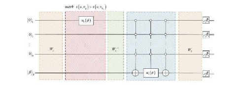
Having obtained the state |βpsubscriptket𝛽𝑝{\left|\beta\right\rangle_{p}} (see Eq. (20)) through the amplitude estimation, we introduce a quantum minimum search algorithm [37] to find k𝑘k nearest neighbor samples from Class C¯psubscript¯𝐶𝑝\bar{C}_{p} with the time complexity of O(kMp)𝑂𝑘subscript𝑀𝑝O\left({\sqrt{k{M_{p}}}}\right), and its quantum circuit is shown in Fig. 6.
Refer to caption

Figure 6: Quantum circuit of finding k𝑘k nearest neighbor samples.

Suppose the set K={K1,K2,,Kk}𝐾subscript𝐾1subscript𝐾2subscript𝐾𝑘K=\left\{{{K_{1}},{K_{2}},\cdots,{K_{k}}}\right\} represents the k𝑘k nearest neighbor samples, so we should prepare k𝑘\left\lceil{\sqrt{{k}}}\right\rceil auxiliary qubits. As shown in Fig. 6, the operator Wssubscript𝑊𝑠W_{s} represents Ws|βp|0k=|βp|K1|K2|Kksubscript𝑊𝑠subscriptket𝛽𝑝ketsuperscript0tensor-productabsent𝑘subscriptket𝛽𝑝ketsubscript𝐾1ketsubscript𝐾2ketsubscript𝐾𝑘{W_{s}}{\left|\beta\right\rangle_{p}}\left|{{0^{\otimes k}}}\right\rangle={\left|\beta\right\rangle_{p}}\left|{{K_{1}}}\right\rangle\left|{{K_{2}}}\right\rangle\cdots\left|{{K_{k}}}\right\rangle, and u1(ϕ)subscript𝑢1italic-ϕu_{1}(\phi) is the operator defined in Eq. (22). Let d0=s(u¯,v¯1)subscript𝑑0𝑠¯𝑢subscript¯𝑣1{d_{0}}=s\left({\bar{u},{\bar{v}_{1}}}\right), we can mark Kxsubscript𝐾𝑥{K_{x}} when d0>s(u¯,v¯Kx),x[1,k]formulae-sequencesubscript𝑑0𝑠¯𝑢subscript¯𝑣subscript𝐾𝑥𝑥1𝑘{d_{0}}>s(\bar{u},{\bar{v}_{{K_{x}}}}),x\in[1,k]. Next, we can replace d0subscript𝑑0d_{0} after one iteration, where d0subscript𝑑0d_{0} is min{s(u¯,v¯Kx)}𝑠¯𝑢subscript¯𝑣subscript𝐾𝑥\min\{s(\bar{u},{\bar{v}_{{K_{x}}}})\}, x[1,k]𝑥1𝑘x\in[1,k]. We repeat the above steps several times until all samples in Class C¯psubscript¯𝐶𝑝\bar{C}_{p} are compared. Finally, all index of k𝑘k nearest neighbor samples in Class C¯psubscript¯𝐶𝑝\bar{C}_{p} can be gotten according to the similarity.

3.4 Updating weight vector

After the above steps, we obtain the nearest neighbor samples (i.e., Hjsubscript𝐻𝑗H_{j} and Mj(C¯p)subscript𝑀𝑗subscript¯𝐶𝑝{M_{j}}(\bar{C}_{p})) of the random sample u¯¯𝑢\bar{u}. Then, we update the weight vector according to the updating weight vector formula as follows,

WT[i]=WT[i]j=1kdiff(i,u¯,Hj)+C¯pclass(u¯)[p(C¯p)1p(class(u¯))j=1kdiff(i,u¯,Mj(C¯p))],𝑊𝑇delimited-[]𝑖𝑊𝑇delimited-[]𝑖superscriptsubscript𝑗1𝑘𝑑𝑖𝑓𝑓𝑖¯𝑢subscript𝐻𝑗subscriptsubscript¯𝐶𝑝𝑐𝑙𝑎𝑠𝑠¯𝑢delimited-[]𝑝subscript¯𝐶𝑝1𝑝𝑐𝑙𝑎𝑠𝑠¯𝑢superscriptsubscript𝑗1𝑘𝑑𝑖𝑓𝑓𝑖¯𝑢subscript𝑀𝑗subscript¯𝐶𝑝\begin{gathered}WT\left[i\right]=WT\left[i\right]-\sum\limits_{j=1}^{k}{diff(i,\bar{u},{H_{j}})}\hfill\\ +\sum\limits_{{\bar{C}_{p}}\notin class(\bar{u})}{[\frac{{p(\bar{C}_{p})}}{{1-p(class(\bar{u}))}}\sum\limits_{j=1}^{k}{diff(i,\bar{u},{M_{j}}(\bar{C}_{p}))}]}\hfill\\ \end{gathered}, (25)

where i[1,N]𝑖1𝑁i\in[1,N].

3.5 Feature selection

After iterating the above steps, i.e., similarity calculation, find the nearest neighbor samples and update weight vector, T𝑇T times, we jump out of the algorithm’s loop. Then we get a final weight vector WT𝑊𝑇WT. And the average weight vector is,

WT¯=1TWT.¯𝑊𝑇1𝑇𝑊𝑇\overline{WT}={1\over T}WT. (26)

Then, we make feature selection based on the final WT¯¯𝑊𝑇\overline{WT} and threshold τ𝜏\tau. Here, τ𝜏\tau can be chosen to retain relevant features and discard irrelevant features [38], that is to say, those features whose weight greater than τ𝜏\tau will be selected, and those less than τ𝜏\tau will be discarded. Here, the value of τ𝜏\tau is determined with regards to the user’s requirements and the characteristics of the problem itself (e.g., the distribution of samples, the number of features).

4 Example

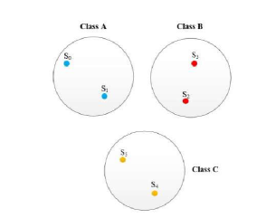
Suppose there are four samples(see Table 1), S0=(1,0,0,1,0,0)subscript𝑆0100100{S_{0}}=(1,0,0,1,0,0), S1=(1,0,0,0,1,0)subscript𝑆1100010{S_{1}}=(1,0,0,0,1,0), S2=(0,1,0,0,0,1)subscript𝑆2010001{S_{2}}=(0,1,0,0,0,1), S3=(0,1,0,1,0,0)subscript𝑆3010100{S_{3}}=(0,1,0,1,0,0), S4=(0,0,1,0,1,0)subscript𝑆4001010{S_{4}}=(0,0,1,0,1,0), S5=(0,0,1,0,0,1)subscript𝑆5001001{S_{5}}=(0,0,1,0,0,1), thus the n𝑛n is 3, and they belong to two classes: A={S0,S1}𝐴subscript𝑆0subscript𝑆1A=\{{S_{0}},{S_{1}}\}, B={S2,S3}𝐵subscript𝑆2subscript𝑆3B=\{{S_{2}},{S_{3}}\}, C={S4,S5}𝐶subscript𝑆4subscript𝑆5C=\{{S_{4}},{S_{5}}\}, which is illustrated in Fig. 7.

Table 1: The feature values of four samples. Each row represents all the feature values of a certain sample, while each column denotes a certain feature value of all the samples
F0subscript𝐹0F_{0} F1subscript𝐹1F_{1} F2subscript𝐹2F_{2} F3subscript𝐹3F_{3} F4subscript𝐹4F_{4} F5subscript𝐹5F_{5}
S0subscript𝑆0S_{0} 1 0 1 0 0 0
S1subscript𝑆1S_{1} 1 0 0 0 1 0
S2subscript𝑆2S_{2} 0 1 0 0 0 1
S3subscript𝑆3S_{3} 0 1 0 1 0 0
S4subscript𝑆4S_{4} 0 0 1 0 1 0
S5subscript𝑆5S_{5} 0 0 1 0 0 1
Refer to caption
Figure 7: The simple example with six samples in classes A𝐴A, B𝐵B and C𝐶C.

First, the four initial quantum states are prepared as follows,

{|ψS0=|000|03|1|0|ψS1=|001|03|1|0|ψS2=|010|03|1|0|ψS3=|011|03|1|0|ψS4=|100|03|1|0|ψS5=|100|03|1|0.casessubscriptket𝜓subscriptS0ket000superscriptket0tensor-productabsent3ket1ket0missing-subexpressionmissing-subexpressionmissing-subexpressionmissing-subexpressionmissing-subexpressionmissing-subexpressionmissing-subexpressionmissing-subexpressionmissing-subexpressionmissing-subexpressionmissing-subexpressionmissing-subexpressionmissing-subexpressionmissing-subexpressionmissing-subexpressionmissing-subexpressionmissing-subexpressionmissing-subexpressionmissing-subexpressionsubscriptket𝜓subscriptS1ket001superscriptket0tensor-productabsent3ket1ket0missing-subexpressionmissing-subexpressionmissing-subexpressionmissing-subexpressionmissing-subexpressionmissing-subexpressionmissing-subexpressionmissing-subexpressionmissing-subexpressionmissing-subexpressionmissing-subexpressionmissing-subexpressionmissing-subexpressionmissing-subexpressionmissing-subexpressionmissing-subexpressionmissing-subexpressionmissing-subexpressionmissing-subexpressionsubscriptket𝜓subscriptS2ket010superscriptket0tensor-productabsent3ket1ket0missing-subexpressionmissing-subexpressionmissing-subexpressionmissing-subexpressionmissing-subexpressionmissing-subexpressionmissing-subexpressionmissing-subexpressionmissing-subexpressionmissing-subexpressionmissing-subexpressionmissing-subexpressionmissing-subexpressionmissing-subexpressionmissing-subexpressionmissing-subexpressionmissing-subexpressionmissing-subexpressionmissing-subexpressionsubscriptket𝜓subscriptS3ket011superscriptket0tensor-productabsent3ket1ket0missing-subexpressionmissing-subexpressionmissing-subexpressionmissing-subexpressionmissing-subexpressionmissing-subexpressionmissing-subexpressionmissing-subexpressionmissing-subexpressionmissing-subexpressionmissing-subexpressionmissing-subexpressionmissing-subexpressionmissing-subexpressionmissing-subexpressionmissing-subexpressionmissing-subexpressionmissing-subexpressionmissing-subexpressionsubscriptket𝜓subscriptS4ket100superscriptket0tensor-productabsent3ket1ket0missing-subexpressionmissing-subexpressionmissing-subexpressionmissing-subexpressionmissing-subexpressionmissing-subexpressionmissing-subexpressionmissing-subexpressionmissing-subexpressionmissing-subexpressionmissing-subexpressionmissing-subexpressionmissing-subexpressionmissing-subexpressionmissing-subexpressionmissing-subexpressionmissing-subexpressionmissing-subexpressionmissing-subexpressionsubscriptket𝜓subscriptS5ket100superscriptket0tensor-productabsent3ket1ket0missing-subexpressionmissing-subexpressionmissing-subexpressionmissing-subexpressionmissing-subexpressionmissing-subexpressionmissing-subexpressionmissing-subexpressionmissing-subexpressionmissing-subexpressionmissing-subexpressionmissing-subexpressionmissing-subexpressionmissing-subexpressionmissing-subexpressionmissing-subexpressionmissing-subexpressionmissing-subexpressionmissing-subexpression\left\{{\begin{array}[]{*{20}{c}}{\left|\psi\right\rangle_{{{\rm{S}}_{\rm{0}}}}}=\left|{{\rm{000}}}\right\rangle{\left|{\rm{0}}\right\rangle^{\otimes 3}}\left|1\right\rangle\left|0\right\rangle\\ {\left|\psi\right\rangle_{{{\rm{S}}_{\rm{1}}}}}=\left|{{\rm{001}}}\right\rangle{\left|{\rm{0}}\right\rangle^{\otimes 3}}\left|1\right\rangle\left|0\right\rangle\\ {\left|\psi\right\rangle_{{{\rm{S}}_{\rm{2}}}}}=\left|{{\rm{010}}}\right\rangle{\left|{\rm{0}}\right\rangle^{\otimes 3}}\left|1\right\rangle\left|0\right\rangle\\ {\left|\psi\right\rangle_{{{\rm{S}}_{\rm{3}}}}}=\left|{{\rm{011}}}\right\rangle{\left|{\rm{0}}\right\rangle^{\otimes 3}}\left|1\right\rangle\left|0\right\rangle\\ {\left|\psi\right\rangle_{{{\rm{S}}_{\rm{4}}}}}=\left|{{\rm{100}}}\right\rangle{\left|{\rm{0}}\right\rangle^{\otimes 3}}\left|1\right\rangle\left|0\right\rangle\\ {\left|\psi\right\rangle_{{{\rm{S}}_{\rm{5}}}}}=\left|{{\rm{100}}}\right\rangle{\left|{\rm{0}}\right\rangle^{\otimes 3}}\left|1\right\rangle\left|0\right\rangle\end{array}}.\right. (27)

Next, we take |ψS0subscriptket𝜓subscriptS0{\left|\psi\right\rangle_{{{\rm{S}}_{\rm{0}}}}} as an example, then the H3superscript𝐻tensor-productabsent3{H^{\otimes 3}} operation is applied on the third and fourth qubits,

|000|03|1|0H312|000i=03|i|1|0.superscript𝐻tensor-productabsent3ket000superscriptket0tensor-productabsent3ket1ket012ket000superscriptsubscript𝑖03ket𝑖ket1ket0\begin{array}[]{l}\left|{{\rm{000}}}\right\rangle{\left|{\rm{0}}\right\rangle^{\otimes 3}}\left|1\right\rangle\left|0\right\rangle\xrightarrow{H^{\otimes 3}}{1\over 2}\left|{{\rm{000}}}\right\rangle\sum\limits_{i=0}^{3}{\left|i\right\rangle\left|1\right\rangle\left|0\right\rangle}\end{array}. (28)

Then we perform Rysubscript𝑅𝑦{R_{y}} rotation (see Eq. (9)) on the last qubit, and can get

|ϕS0=12|000i=03|i|1(1|v¯0i|2|0+v¯0i|1).subscriptketitalic-ϕsubscriptS012ket000superscriptsubscript𝑖03ket𝑖ket11superscriptsubscript¯𝑣0𝑖2ket0subscript¯𝑣0𝑖ket1{\left|\phi\right\rangle_{{{\rm{S}}_{\rm{0}}}}}={1\over 2}\left|{{\rm{000}}}\right\rangle\sum\limits_{i=0}^{3}{\left|i\right\rangle\left|1\right\rangle\left({\sqrt{{\rm{1-}}{{\left|{{\bar{v}_{0i}}}\right|}^{2}}}\left|0\right\rangle+{\bar{v}_{0i}}\left|1\right\rangle}\right)}. (29)

The other quantum states are prepared in the same way and they are listed as below,

{|ϕS0=12|000i=03|i|1(1|v¯0i|2|0+v¯0i|1)|ϕS1=12|001i=03|i|1(1|v¯1i|2|0+v¯1i|1)|ϕS2=12|010i=03|i|1(1|v¯2i|2|0+v¯2i|1)|ϕS3=12|011i=03|i|1(1|v¯3i|2|0+v¯3i|1)|ϕS4=12|100i=03|i|1(1|v¯4i|2|0+v¯4i|1)|ϕS5=12|101i=03|i|1(1|v¯5i|2|0+v¯5i|1).casessubscriptketitalic-ϕsubscript𝑆012ket000superscriptsubscript𝑖03ket𝑖ket11superscriptsubscript¯𝑣0𝑖2ket0subscript¯𝑣0𝑖ket1missing-subexpressionmissing-subexpressionmissing-subexpressionmissing-subexpressionmissing-subexpressionmissing-subexpressionmissing-subexpressionmissing-subexpressionmissing-subexpressionmissing-subexpressionmissing-subexpressionmissing-subexpressionmissing-subexpressionmissing-subexpressionmissing-subexpressionmissing-subexpressionmissing-subexpressionmissing-subexpressionmissing-subexpressionsubscriptketitalic-ϕsubscript𝑆112ket001superscriptsubscript𝑖03ket𝑖ket11superscriptsubscript¯𝑣1𝑖2ket0subscript¯𝑣1𝑖ket1missing-subexpressionmissing-subexpressionmissing-subexpressionmissing-subexpressionmissing-subexpressionmissing-subexpressionmissing-subexpressionmissing-subexpressionmissing-subexpressionmissing-subexpressionmissing-subexpressionmissing-subexpressionmissing-subexpressionmissing-subexpressionmissing-subexpressionmissing-subexpressionmissing-subexpressionmissing-subexpressionmissing-subexpressionsubscriptketitalic-ϕsubscript𝑆212ket010superscriptsubscript𝑖03ket𝑖ket11superscriptsubscript¯𝑣2𝑖2ket0subscript¯𝑣2𝑖ket1missing-subexpressionmissing-subexpressionmissing-subexpressionmissing-subexpressionmissing-subexpressionmissing-subexpressionmissing-subexpressionmissing-subexpressionmissing-subexpressionmissing-subexpressionmissing-subexpressionmissing-subexpressionmissing-subexpressionmissing-subexpressionmissing-subexpressionmissing-subexpressionmissing-subexpressionmissing-subexpressionmissing-subexpressionsubscriptketitalic-ϕsubscript𝑆312ket011superscriptsubscript𝑖03ket𝑖ket11superscriptsubscript¯𝑣3𝑖2ket0subscript¯𝑣3𝑖ket1missing-subexpressionmissing-subexpressionmissing-subexpressionmissing-subexpressionmissing-subexpressionmissing-subexpressionmissing-subexpressionmissing-subexpressionmissing-subexpressionmissing-subexpressionmissing-subexpressionmissing-subexpressionmissing-subexpressionmissing-subexpressionmissing-subexpressionmissing-subexpressionmissing-subexpressionmissing-subexpressionmissing-subexpressionsubscriptketitalic-ϕsubscript𝑆412ket100superscriptsubscript𝑖03ket𝑖ket11superscriptsubscript¯𝑣4𝑖2ket0subscript¯𝑣4𝑖ket1missing-subexpressionmissing-subexpressionmissing-subexpressionmissing-subexpressionmissing-subexpressionmissing-subexpressionmissing-subexpressionmissing-subexpressionmissing-subexpressionmissing-subexpressionmissing-subexpressionmissing-subexpressionmissing-subexpressionmissing-subexpressionmissing-subexpressionmissing-subexpressionmissing-subexpressionmissing-subexpressionmissing-subexpressionsubscriptketitalic-ϕsubscript𝑆512ket101superscriptsubscript𝑖03ket𝑖ket11superscriptsubscript¯𝑣5𝑖2ket0subscript¯𝑣5𝑖ket1missing-subexpressionmissing-subexpressionmissing-subexpressionmissing-subexpressionmissing-subexpressionmissing-subexpressionmissing-subexpressionmissing-subexpressionmissing-subexpressionmissing-subexpressionmissing-subexpressionmissing-subexpressionmissing-subexpressionmissing-subexpressionmissing-subexpressionmissing-subexpressionmissing-subexpressionmissing-subexpressionmissing-subexpression\left\{{\begin{array}[]{*{20}{c}}{\left|\phi\right\rangle_{{S_{0}}}}={1\over 2}\left|{000}\right\rangle\sum\limits_{i=0}^{3}{\left|i\right\rangle}\left|1\right\rangle\left({\sqrt{1-{{\left|{{\bar{v}_{0i}}}\right|}^{2}}}\left|0\right\rangle+{\bar{v}_{0i}}\left|1\right\rangle}\right)\\ {\left|\phi\right\rangle_{{S_{1}}}}={1\over 2}\left|{001}\right\rangle\sum\limits_{i=0}^{3}{\left|i\right\rangle}\left|1\right\rangle\left({\sqrt{1-{{\left|{{\bar{v}_{1i}}}\right|}^{2}}}\left|0\right\rangle+{\bar{v}_{1i}}\left|1\right\rangle}\right)\\ {\left|\phi\right\rangle_{{S_{2}}}}={1\over 2}\left|{010}\right\rangle\sum\limits_{i=0}^{3}{\left|i\right\rangle}\left|1\right\rangle\left({\sqrt{1-{{\left|{{\bar{v}_{2i}}}\right|}^{2}}}\left|0\right\rangle+{\bar{v}_{2i}}\left|1\right\rangle}\right)\\ {\left|\phi\right\rangle_{{S_{3}}}}={1\over 2}\left|{011}\right\rangle\sum\limits_{i=0}^{3}{\left|i\right\rangle}\left|1\right\rangle\left({\sqrt{1-{{\left|{{\bar{v}_{3i}}}\right|}^{2}}}\left|0\right\rangle+{\bar{v}_{3i}}\left|1\right\rangle}\right)\\ {\left|\phi\right\rangle_{{S_{4}}}}={1\over 2}\left|{100}\right\rangle\sum\limits_{i=0}^{3}{\left|i\right\rangle}\left|1\right\rangle\left({\sqrt{1-{{\left|{{\bar{v}_{4i}}}\right|}^{2}}}\left|0\right\rangle+{\bar{v}_{4i}}\left|1\right\rangle}\right)\\ {\left|\phi\right\rangle_{{S_{5}}}}={1\over 2}\left|{101}\right\rangle\sum\limits_{i=0}^{3}{\left|i\right\rangle}\left|1\right\rangle\left({\sqrt{1-{{\left|{{\bar{v}_{5i}}}\right|}^{2}}}\left|0\right\rangle+{\bar{v}_{5i}}\left|1\right\rangle}\right)\end{array}}.\right. (30)

Second, we randomly select a sample (assume |ϕS0subscriptketitalic-ϕsubscriptS0{\left|\phi\right\rangle_{{{\rm{S}}_{\rm{0}}}}} is u¯¯𝑢\bar{u}), and perform similarity calculation with other samples (i.e., |ϕS1subscriptketitalic-ϕsubscriptS1{\left|\phi\right\rangle_{{{\rm{S}}_{\rm{1}}}}}, |ϕS2subscriptketitalic-ϕsubscriptS2{\left|\phi\right\rangle_{{{\rm{S}}_{\rm{2}}}}}, |ϕS3subscriptketitalic-ϕsubscriptS3{\left|\phi\right\rangle_{{{\rm{S}}_{\rm{3}}}}}, |ϕS4subscriptketitalic-ϕsubscriptS4{\left|\phi\right\rangle_{{{\rm{S}}_{\rm{4}}}}}, |ϕS5subscriptketitalic-ϕsubscriptS5{\left|\phi\right\rangle_{{{\rm{S}}_{\rm{5}}}}}). Next, we take |ϕS0subscriptketitalic-ϕsubscriptS0{\left|\phi\right\rangle_{{{\rm{S}}_{\rm{0}}}}} and |ϕS1subscriptketitalic-ϕsubscriptS1{\left|\phi\right\rangle_{{{\rm{S}}_{\rm{1}}}}} as an example, and perform a swap operation between the last two qubits of |ϕS0subscriptketitalic-ϕsubscriptS0{\left|\phi\right\rangle_{{{\rm{S}}_{\rm{0}}}}},

|ϕS0swap|φ=12|000i=03|i(1|v¯0i|2|0+v¯0i|1)|1.𝑠𝑤𝑎𝑝subscriptketitalic-ϕsubscriptS0ket𝜑12ket000superscriptsubscript𝑖03ket𝑖1superscriptsubscript¯𝑣0𝑖2ket0subscript¯𝑣0𝑖ket1ket1\begin{array}[]{l}{\left|\phi\right\rangle_{{{\rm{S}}_{\rm{0}}}}}\xrightarrow{swap}\left|{{\varphi}}\right\rangle={1\over 2}\left|{{\rm{000}}}\right\rangle\sum\limits_{i=0}^{3}{\left|i\right\rangle\left({\sqrt{{\rm{1-}}{{\left|{{\bar{v}_{0i}}}\right|}^{2}}}\left|0\right\rangle+{\bar{v}_{0i}}\left|1\right\rangle}\right)\left|1\right\rangle}\end{array}. (31)

After that, the swap test operation is applied on (|φket𝜑\left|{{\varphi}}\right\rangle, |ϕS1subscriptketitalic-ϕsubscriptS1\left|{{\phi}}\right\rangle_{{{\rm{S}}_{\rm{1}}}}),

12|0(|φ|ϕS1+|ϕS1|φ)+12|1(|φ|ϕS1|ϕS1|φ).12ket0ket𝜑subscriptketitalic-ϕsubscriptS1subscriptketitalic-ϕsubscriptS1ket𝜑12ket1ket𝜑subscriptketitalic-ϕsubscriptS1subscriptketitalic-ϕsubscriptS1ket𝜑\begin{array}[]{l}{1\over 2}\left|0\right\rangle\left({\left|\varphi\right\rangle{{\left|{{\phi}}\right\rangle_{{{\rm{S}}_{\rm{1}}}}}}+{{\left|{{\phi}}\right\rangle_{{{\rm{S}}_{\rm{1}}}}}}\left|\varphi\right\rangle}\right)+{1\over 2}\left|1\right\rangle\left({{\left|\varphi\right\rangle{\left|{{\phi}}\right\rangle_{{{\rm{S}}_{\rm{1}}}}}}-{{\left|{{\phi}}\right\rangle_{{{\rm{S}}_{\rm{1}}}}}}\left|\varphi\right\rangle}\right)\\ \end{array}. (32)

We perform a swap test operation to obtain a quantum state that encodes similarity in amplitude£¬

{|αA=12q=12|q(1s(u¯,v¯q)|0+s(u¯,v¯q)|1)|αB=12q=12|q(1s(u¯,v¯q)|0+s(u¯,v¯q)|1)|αC=12q=12|q(1s(u¯,v¯q)|0+s(u¯,v¯q)|1).casessubscriptket𝛼𝐴12superscriptsubscript𝑞12ket𝑞1𝑠¯𝑢subscript¯𝑣𝑞ket0𝑠¯𝑢subscript¯𝑣𝑞ket1missing-subexpressionmissing-subexpressionmissing-subexpressionmissing-subexpressionmissing-subexpressionmissing-subexpressionmissing-subexpressionmissing-subexpressionmissing-subexpressionmissing-subexpressionmissing-subexpressionmissing-subexpressionmissing-subexpressionmissing-subexpressionmissing-subexpressionmissing-subexpressionmissing-subexpressionmissing-subexpressionmissing-subexpressionsubscriptket𝛼𝐵12superscriptsubscript𝑞12ket𝑞1𝑠¯𝑢subscript¯𝑣𝑞ket0𝑠¯𝑢subscript¯𝑣𝑞ket1missing-subexpressionmissing-subexpressionmissing-subexpressionmissing-subexpressionmissing-subexpressionmissing-subexpressionmissing-subexpressionmissing-subexpressionmissing-subexpressionmissing-subexpressionmissing-subexpressionmissing-subexpressionmissing-subexpressionmissing-subexpressionmissing-subexpressionmissing-subexpressionmissing-subexpressionmissing-subexpressionmissing-subexpressionsubscriptket𝛼𝐶12superscriptsubscript𝑞12ket𝑞1𝑠¯𝑢subscript¯𝑣𝑞ket0𝑠¯𝑢subscript¯𝑣𝑞ket1missing-subexpressionmissing-subexpressionmissing-subexpressionmissing-subexpressionmissing-subexpressionmissing-subexpressionmissing-subexpressionmissing-subexpressionmissing-subexpressionmissing-subexpressionmissing-subexpressionmissing-subexpressionmissing-subexpressionmissing-subexpressionmissing-subexpressionmissing-subexpressionmissing-subexpressionmissing-subexpressionmissing-subexpression\left\{{\begin{array}[]{*{20}{c}}{\left|\alpha\right\rangle_{A}}={1\over{\sqrt{2}}}\sum\limits_{q=1}^{2}{\left|q\right\rangle}\left({\sqrt{1-s(\bar{u},{\bar{v}_{q}})}\left|0\right\rangle+\sqrt{s(\bar{u},{\bar{v}_{q}})}\left|1\right\rangle}\right)\\ {\left|\alpha\right\rangle_{B}}={1\over{\sqrt{2}}}\sum\limits_{q=1}^{2}{\left|q\right\rangle}\left({\sqrt{1-s(\bar{u},{\bar{v}_{q}})}\left|0\right\rangle+\sqrt{s(\bar{u},{\bar{v}_{q}})}\left|1\right\rangle}\right)\\ {\left|\alpha\right\rangle_{C}}={1\over{\sqrt{2}}}\sum\limits_{q=1}^{2}{\left|q\right\rangle}\left({\sqrt{1-s(\bar{u},{\bar{v}_{q}})}\left|0\right\rangle+\sqrt{s(\bar{u},{\bar{v}_{q}})}\left|1\right\rangle}\right)\end{array}}.\right. (33)

Then through the amplitude estimation, we can obtain the quantum states,

{|βA=12q=12|q|v¯qu¯|βB=12q=12|q|v¯qu¯|βC=12q=12|q|v¯qu¯.casessubscriptket𝛽𝐴12superscriptsubscript𝑞12ket𝑞ketsubscript¯𝑣𝑞¯𝑢missing-subexpressionmissing-subexpressionmissing-subexpressionmissing-subexpressionmissing-subexpressionmissing-subexpressionmissing-subexpressionmissing-subexpressionmissing-subexpressionmissing-subexpressionmissing-subexpressionmissing-subexpressionmissing-subexpressionmissing-subexpressionmissing-subexpressionmissing-subexpressionmissing-subexpressionmissing-subexpressionmissing-subexpressionsubscriptket𝛽𝐵12superscriptsubscript𝑞12ket𝑞ketsubscript¯𝑣𝑞¯𝑢missing-subexpressionmissing-subexpressionmissing-subexpressionmissing-subexpressionmissing-subexpressionmissing-subexpressionmissing-subexpressionmissing-subexpressionmissing-subexpressionmissing-subexpressionmissing-subexpressionmissing-subexpressionmissing-subexpressionmissing-subexpressionmissing-subexpressionmissing-subexpressionmissing-subexpressionmissing-subexpressionmissing-subexpressionsubscriptket𝛽𝐶12superscriptsubscript𝑞12ket𝑞ketsubscript¯𝑣𝑞¯𝑢missing-subexpressionmissing-subexpressionmissing-subexpressionmissing-subexpressionmissing-subexpressionmissing-subexpressionmissing-subexpressionmissing-subexpressionmissing-subexpressionmissing-subexpressionmissing-subexpressionmissing-subexpressionmissing-subexpressionmissing-subexpressionmissing-subexpressionmissing-subexpressionmissing-subexpressionmissing-subexpressionmissing-subexpression\left\{{\begin{array}[]{*{20}{c}}{\left|\beta\right\rangle_{A}}={1\over{\sqrt{2}}}\sum\limits_{q=1}^{2}{\left|q\right\rangle}\left|{{\bar{v}_{q}}-\bar{u}}\right\rangle\\ {\left|\beta\right\rangle_{B}}={1\over{\sqrt{2}}}\sum\limits_{q=1}^{2}{\left|q\right\rangle}\left|{{\bar{v}_{q}}-\bar{u}}\right\rangle\\ {\left|\beta\right\rangle_{C}}={1\over{\sqrt{2}}}\sum\limits_{q=1}^{2}{\left|q\right\rangle}\left|{{\bar{v}_{q}}-\bar{u}}\right\rangle\end{array}}.\right. (34)

Next, we perform an oracle operation on the quantum states obtained in the above steps to obtain the k𝑘k nearest neighbor samples.

5 Simulation Experiment

Quantum Cloud Services (QCSTM𝑄𝐶superscript𝑆𝑇𝑀QC{S^{TM}}) is Rigetti’s quantum-first cloud computing platform. At the end of 2017, a 19-qubit processor named ‘Acorn’ was launched, which can be used in QCS through a quantum programming toolkit named Forest [39]. The chip of ‘Acorn’ is made of 20 superconducting qubits but for some technical reasons, qubit 3 is off-line and cannot interact with its neighbors, so it is treated as a 19-qubit device whose coupling map is shown in Fig. 8.

Refer to caption

Figure 8: The coupling map picture: Rigetti’s 19-qubit processor ‘Acorn’. Lines indicate the two-qubit connection ruled by a controlled-Z𝑍Z operation.

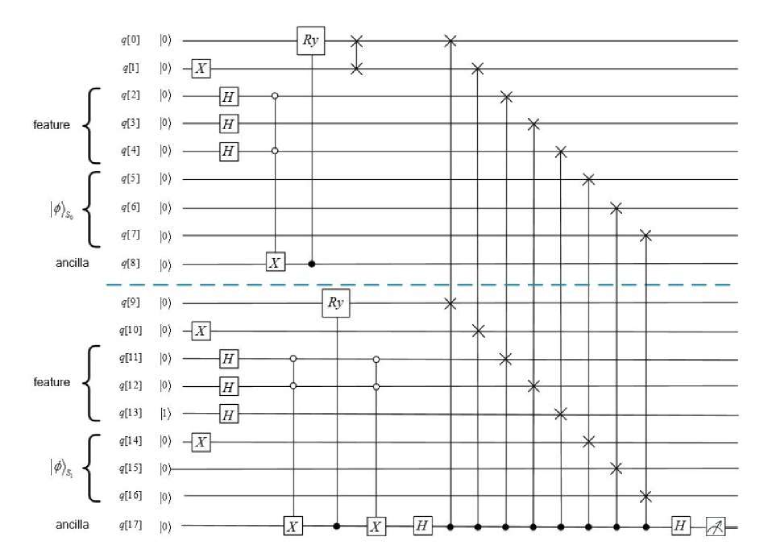
In order to obtain the result and also verify our algorithm, we choose Rigetti to perform the quantum processing. However, since the Rigetti platform limits the length of the entire circuit and noise has a great influence on the preparation of quantum states [40], we only show one of the ideal experiment circuits of similarity calculation in QReliefF algorithm running on Rigetti platform. We successfully stored the characteristic information in the sample into the amplitude of the quantum state, and then extracted the amplitude information into the quantum state through the phase estimation algorithm. Fig. 9 gives the schematic diagram of our experimental circuit.
Refer to caption
Figure 9: One of the ideal experiment circuits of similarity calculation in QReliefF algorithm running on Rigetti platform. q[0]q[7]𝑞delimited-[]0𝑞delimited-[]7q[0]-q[7] represents the randomly selected quantum state |ϕS0subscriptketitalic-ϕsubscript𝑆0\left|{{\phi}}\right\rangle_{S_{0}}, q[9]q[16]𝑞delimited-[]9𝑞delimited-[]16q[9]-q[16] represents |ϕS1subscriptketitalic-ϕsubscript𝑆1\left|{{\phi}}\right\rangle_{S_{1}}, and q[17]𝑞delimited-[]17q[17] is the result qubit. X is the Not operation, and Ry is Rysubscript𝑅𝑦{R_{y}} operation which can be expressed as a matrix in Eq. (9).

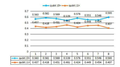
The corresponding code of the circuit in Riggeti is shown in Program 3. After running 888 times of Program 3, the result can be seen in Fig. 10. We can get |1ket1\left|1\right\rangle with the average probability of 0.435125. Then we successfully stored the characteristic information in the sample into the amplitude of the quantum state. According to Eq. (33), we can get s(u¯,v¯q)0.435𝑠¯𝑢subscript¯𝑣𝑞0.435\sqrt{s\left({\bar{u},{\bar{v}_{q}}}\right)}\approx\sqrt{0.435}, i.e., s(u¯,v¯q)0.435𝑠¯𝑢subscript¯𝑣𝑞0.435s\left({\bar{u},{\bar{v}_{q}}}\right)\approx 0.435, and then extracted the amplitude information into the quantum state through the phase estimation algorithm.
1        # Define the new gate from a matrix
2theta=Parameter(theta)\;\;\;\;\;\;\;theta=Parameter(^{\prime}theta^{\prime})
3cry=np.array([\;\;\;\;\;\;\;cry=np.array([
4[1,0,0,0],1000\;\;\;\;\;\;\;\;\;\;\;\;\;\;\;\;[1,0,0,0],
5[0,1,0,0],0100\;\;\;\;\;\;\;\;\;\;\;\;\;\;\;\;[0,1,0,0],
6[0,0,quil_sqrt(1thetatheta),thetatheta],00𝑞𝑢𝑖𝑙_𝑠𝑞𝑟𝑡1𝑡𝑒𝑡𝑎𝑡𝑒𝑡𝑎𝑡𝑒𝑡𝑎𝑡𝑒𝑡𝑎\;\;\;\;\;\;\;\;\;\;\;\;\;\;\;\;[0,0,quil\_sqrt(1-theta*theta),-theta*theta],
7[0,0,thetatheta,quil_sqrt(1thetatheta)]00𝑡𝑒𝑡𝑎𝑡𝑒𝑡𝑎𝑞𝑢𝑖𝑙_𝑠𝑞𝑟𝑡1𝑡𝑒𝑡𝑎𝑡𝑒𝑡𝑎\;\;\;\;\;\;\;\;\;\;\;\;\;\;\;\;[0,0,theta*theta,quil\_sqrt(1-theta*theta)]
8])\;\;\;\;\;\;\;]);
9
10gate_definition=DefGate(CRY,cry,[theta])\;\;\;\;\;\;\;gate\_definition=DefGate(^{\prime}CRY^{\prime},cry,[theta])
11CRY=gate_definition.get_constructor()formulae-sequence𝐶𝑅𝑌𝑔𝑎𝑡𝑒_𝑑𝑒𝑓𝑖𝑛𝑖𝑡𝑖𝑜𝑛𝑔𝑒𝑡_𝑐𝑜𝑛𝑠𝑡𝑟𝑢𝑐𝑡𝑜𝑟\;\;\;\;\;\;\;CRY=gate\_definition.get\_constructor()
12       # Create our program and use the new parametric gate
13p=Program(\;\;\;\;\;\;\;p=Program(
14gate_definition,X(1),H(2),H(4),H(5),X(2),X(5),𝑔𝑎𝑡𝑒_𝑑𝑒𝑓𝑖𝑛𝑖𝑡𝑖𝑜𝑛𝑋1𝐻2𝐻4𝐻5𝑋2𝑋5\;\;\;\;\;\;\;\;\;\;gate\_definition,X(1),H(2),H(4),H(5),X(2),X(5),
15CCNOT(2,5,18),X(2),X(5),CRY(1)(18,0),𝐶𝐶𝑁𝑂𝑇2518𝑋2𝑋5𝐶𝑅𝑌1180\;\;\;\;\;\;\;\;\;\;CCNOT(2,5,18),X(2),X(5),CRY(1)(18,0),
16SWAP(0,1),X(10),H(11),H(12),H(13),X(14),𝑆𝑊𝐴𝑃01𝑋10𝐻11𝐻12𝐻13𝑋14\;\;\;\;\;\;\;\;\;\;SWAP(0,1),X(10),H(11),H(12),H(13),X(14),
17X(11),X(12),CCNOT(11,12,17),X(11),X(12),𝑋11𝑋12𝐶𝐶𝑁𝑂𝑇111217𝑋11𝑋12\;\;\;\;\;\;\;\;\;\;X(11),X(12),CCNOT(11,12,17),X(11),X(12),
18CRY(1)(17,9),H(19),CSWAP(19,0,9),𝐶𝑅𝑌1179𝐻19𝐶𝑆𝑊𝐴𝑃1909\;\;\;\;\;\;\;\;\;\;CRY(1)(17,9),H(19),CSWAP(19,0,9),
19CSWAP(19,1,10),CSWAP(19,2,11),𝐶𝑆𝑊𝐴𝑃19110𝐶𝑆𝑊𝐴𝑃19211\;\;\;\;\;\;\;\;\;\;CSWAP(19,1,10),CSWAP(19,2,11),
20CSWAP(19,4,12),CSWAP(19,5,13),𝐶𝑆𝑊𝐴𝑃19412𝐶𝑆𝑊𝐴𝑃19513\;\;\;\;\;\;\;\;\;\;CSWAP(19,4,12),CSWAP(19,5,13),
21CSWAP(19,6,14),CSWAP(19,7,15),𝐶𝑆𝑊𝐴𝑃19614𝐶𝑆𝑊𝐴𝑃19715\;\;\;\;\;\;\;\;\;\;CSWAP(19,6,14),CSWAP(19,7,15),
22CSWAP(19,8,16),H(19)𝐶𝑆𝑊𝐴𝑃19816𝐻19\;\;\;\;\;\;\;\;\;\;CSWAP(19,8,16),H(19)
23))\;\;\;\;\;\;\;)
24       #print the circuit
25print(p)𝑝𝑟𝑖𝑛𝑡𝑝\;\;\;\;\;\;\;print(p)
26       # get a QPU, 20q-Acorn is just a string naming the device
27qc=get_qc(20qAcorn)\;\;\;\;\;\;\;qc=get\_qc(^{\prime}20q-Acorn^{\prime})
28       # run and measure
result=qc.run_and_measure(p,trials=1024)formulae-sequence𝑟𝑒𝑠𝑢𝑙𝑡𝑞𝑐𝑟𝑢𝑛_𝑎𝑛𝑑_𝑚𝑒𝑎𝑠𝑢𝑟𝑒𝑝𝑡𝑟𝑖𝑎𝑙𝑠1024\;\;\;\;\;\;\;result=qc.run\_and\_measure(p,trials=1024)
Program 3 Similarity calculation in QReliefF algorithm running on Rigetti
Refer to caption
Figure 10: The measurement result of |0ket0\left|0\right\rangle and |1ket1\left|1\right\rangle after running 8 times of Program 3 on Rigetti.

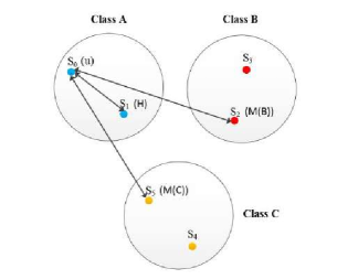
After all the steps have been performed, we obtain the quantum states S1(H)subscript𝑆1𝐻{S_{1}}\;(H), S2(M(B))subscript𝑆2𝑀𝐵{S_{2}}\;(M(B)) and S5(M(C))subscript𝑆5𝑀𝐶{S_{5}}\;(M(C)) of the nearest neighbor samples of the quantum state S0(u¯)subscript𝑆0¯𝑢{S_{0}}\;(\bar{u}) in each class of the random sample which can be seen in Fig. 11. Then, the weight vectors are updated according to Eq. (25) and the result of WT𝑊𝑇WT is listed in the second row of Table 2 after the first iteration.
Refer to caption
Figure 11: Finding the nearest neighbor samples (S1subscript𝑆1{S_{1}}, S2subscript𝑆2{S_{2}} and S5subscript𝑆5{S_{5}}) of the sample S0subscript𝑆0{S_{0}}.
Table 2: The updated result of WT𝑊𝑇WT
Iterationtimes(T)𝐼𝑡𝑒𝑟𝑎𝑡𝑖𝑜𝑛𝑡𝑖𝑚𝑒𝑠𝑇Iterationtimes(T) Weightvector(WT)𝑊𝑒𝑖𝑔𝑡𝑣𝑒𝑐𝑡𝑜𝑟𝑊𝑇Weightvector(WT)
1 [1 1 1 0 0 -1]
2 [2 2 2 -1 0 -1]
3 [3 3 3 -1 0 -2]
4 [4 4 4 -2 0 -2]

The algorithm iterates T𝑇T times (in our example, T𝑇T=4) as above steps, and obtains all the WT𝑊𝑇WT results shown in Table 2. After T𝑇T-th iterations, WT=[4,4,4,2,0,2]𝑊𝑇444202WT=[4,4,4,-2,0,-2], then WT¯=[1,1,1,1/2,0,1/2]¯𝑊𝑇11112012\overline{WT}=[1,1,1,-1/2,0,-1/2]. In this paper, the value of τ𝜏\tau in the example is assumed to be 0.5 according to the updated result of WT in TABLE 2. Since the threshold τ=0.5𝜏0.5\tau=0.5, so the selected features are F0subscript𝐹0F_{0}, F1subscript𝐹1F_{1} and F2subscript𝐹2F_{2}, i.e., the first, second and third features. The result of quantum feature selection is consistent with the classical ReliefF algorithm after being verified by python.

In the final weight value comparison, considering the large amount of data in the complex system and the corresponding eigenvalues, the calculation amount required for the comparison after the final result is obtained is also large. In order to meet the requirements of big data and result accuracy, we adopted an optimized quantum maximum and minimum value search algorithm [37] when comparing weights in the last step to help us quickly and accurately select the features we want, so as to better solve the multi-classification problem in complex systems.

In circumstances when we can exactly estimate the ratio of the number of solutions M𝑀M and the searched space N𝑁N, this algorithm can improve the successful probability close to 100%percent100100{\rm{\%}}. Furthermore, it shows an advantage in complexity with large databases and in the operation complexity of constructing oracles.

6 Efficiency analysis

In order to evaluate the efficiency of QReliefF algorithm, three algorithms (i.e., classical Relief, classical ReliefF, quantum Relief algorithms) are selected to compare with our algorithm from three indicators: complexity of similarity calculation (CSC), complexity of finding the nearest neighbor (CFNN) and resource consumption (RC).

In the classic Relief algorithm, it takes O(N)𝑂𝑁O(N) time to calculate the distance between randomly selected samples and any other samples, and then finds the nearest neighbors related to M𝑀M. This process needs to iterate T𝑇T times, so CSC is O(TMN)𝑂𝑇𝑀𝑁O(TMN). Since T𝑇T is a constant, then CSC in the classic Relief algorithm is O(MN)𝑂𝑀𝑁O(MN). As we know, there are totally M𝑀M samples, each with N𝑁N features, so CFNN is O(M)𝑂𝑀O(M) and RC in the classic Relief algorithm is O(MN)𝑂𝑀𝑁O(MN) bits. The classical ReliefF algorithm is similar to the classical Relief algorithm. Since it finds k𝑘k nearest neighbors at once time, so the time complexity is O(kTMN)𝑂𝑘𝑇𝑀𝑁O(kTMN). Then we can simplify CSC to O(MN)𝑂𝑀𝑁O(MN) because k𝑘k and T𝑇T are constants. Besides, CFNN for finding k𝑘k nearest neighbors is O(M)𝑂𝑀O(M). In terms of resource consumption, there are M𝑀M samples, each sample has N𝑁N features, so the resource consumption of the classic ReliefF algorithm is O(MN)𝑂𝑀𝑁O(MN) bits.

In QRelief and QReliefF algorithms, the quantum property is used to calculate the distance from O(N)𝑂𝑁O(N) to O(1)𝑂1O(1), so their CSCs are all O(TM)𝑂𝑇𝑀O(TM). Since T𝑇T is constant, their CSCs can be simplified to O(M)𝑂𝑀O(M). CFNN of QRelief is O(kM)𝑂𝑘𝑀O\left({kM}\right), then it can be simplified to O(M)𝑂𝑀O\left({M}\right) as k𝑘k is constant. While CFNN of QReliefF is kM𝑘𝑀\sqrt{kM} because it uses the quantum Grover-Long method to find k𝑘k nearest neighbor samples which holds a quadratic acceleration. Since k𝑘k is constant, CFNN of QReliefF is O(M)𝑂𝑀O(\sqrt{M}). RC of similarity calculation, finding the nearest neighbor samples and updating weight vector are O(TMlogN)𝑂𝑇𝑀𝑙𝑜𝑔𝑁O(TMlogN), O(TN)𝑂𝑇𝑁O(TN) and O(N)𝑂𝑁O(N), respectively. Therefore, the total complexity is O(TMlogN+TN+N)𝑂𝑇𝑀𝑙𝑜𝑔𝑁𝑇𝑁𝑁O(TMlogN+TN+N), since T𝑇T is constant, then RC of QRelief and QReliefF are all O(MlogN+N)𝑂𝑀𝑙𝑜𝑔𝑁𝑁O(MlogN+N). For multi-features big data in complex systems with edge computing, there is MNmuch-greater-than𝑀𝑁M\gg N, so MNNlogNmuch-greater-than𝑀𝑁𝑁𝑁M\gg{N\over{N-\log N}}, then RC of QRelief and QReliefF can be simplified into O(MlogN)𝑂𝑀𝑙𝑜𝑔𝑁O(MlogN).

For convenience, we list the efficiency comparison of classic Relief algorithm, ReliefF algorithm, quantum Relief algorithm and our algorithm in terms of CSC, CFNN and RC in Table 3. Obviously, our algorithm is superior than classical algorithms (i.e., Relief and ReliefF) in terms of CSC, CFNN and RC, and better than quantum algorithm (i.e., QRelief) in terms of CFNN.

Table 3: Efficiency comparison between classical Relief, classical ReliefF, QRelief and our QReliefF algorithms
Multi-classification CSC CFNN RC
Relief no O(MN)𝑂𝑀𝑁O(MN) O(M)𝑂𝑀O(M) O(MN)𝑂𝑀𝑁O(MN)
ReliefF yes O(MN)𝑂𝑀𝑁O(MN) O(M)𝑂𝑀O(M) O(MN)𝑂𝑀𝑁O(MN)
QRelief no O(M)𝑂𝑀O(M) O(M)𝑂𝑀O(M) O(MlogN)𝑂𝑀𝑙𝑜𝑔𝑁O(MlogN)
QReliefF yes O(M)𝑂𝑀O(M) O(M)𝑂𝑀O(\sqrt{M}) O(MlogN)𝑂𝑀𝑙𝑜𝑔𝑁O(MlogN)

7 Conclusion and discussion

With the rapid development of edge computing technology and quantum machine learning algorithms, researchers began to pay attention to the combination and application of these two fields. In this paper, we use quantum technology to solve the multi-classification problem of feature selection in the complex systems with edge computing, and propose a quantum ReliefF algorithm. Compared to the classic ReliefF algorithm, our algorithm reduces the complexity of similarity calculation from O(MN)𝑂𝑀𝑁O(MN) to O(M)𝑂𝑀O(M), and the complexity of finding the nearest neighbor from O(M)𝑂𝑀O(M) to O(M)𝑂𝑀O(\sqrt{M}). In addition, from the perspective of resource consumption, our algorithm consumes O(MlogN)𝑂𝑀𝑙𝑜𝑔𝑁O(MlogN) qubit, while the classic ReliefF algorithm consumes O(MN)𝑂𝑀𝑁O(MN) bit. Obviously, our algorithm is superior in terms of computational complexity and resource consumption.

It should be noted that our work aims to improve the algorithm efficiency, while the privacy protection of sensitive data is not taken into account. At present, data security has become a focus of attention in the field of artificial intelligence, some solutions for data privacy protection in complex systems with edge computing have been proposed [41][42][43][44]. In our future work, how to improve the efficiency of quantum machine learning algorithms while ensuring the privacy protection of sensitive data, such as [45][46][47][48], will become our direction.

Acknowledgment

The authors would like to express heartfelt gratitude to the anonymous reviewers and editor for their comments that improved the quality of this paper. And the support of all the members of the quantum research group of NUIST & SEU is especially acknowledged, their professional discussions and advices have helped us a lot.

References

  • [1] Roberta Alfieri and Luciano Milanesi, “Complex System,” Springer New York, New York, 2013.
  • [2] Michael Armbrust, Armando Fox, Rean Griffith, Anthony D. Joseph, Randy Katz, Andy Konwinski, Gunho Lee, David A. Patterson, Ariel Rabkin, Ion Stoica and Matei Zaharia, “A View of Cloud Computing,” Communications of the ACM, vol. 53, no. 4, pp. 50-58, 2010.
  • [3] Xu Chen, Lei Jiao, Wenzhong Li and Xiaoming Fu, “Efficient Multi-User Computation Offloading for Mobile-Edge Cloud Computing,” IEEE/ACM Transactions on Networking, vol. 24, no. 5, pp. 2827-2840, 2016.
  • [4] Xiaolong Xu, Shucun Fu, Lianyong Qi, Xuyun Zhang, Qingxiang Liu, Qiang He and Shang Li, “An IoT-Oriented Data Placement Method with Privacy Preservation in Cloud Environment,” Journal of Network and Computer Applications, vol. 124, pp. 148-157, 2018.
  • [5] Lianyong Qi, Yi Chen, Yuan Yuan, Shucun Fu, Xuyun Zhang and Xiaolong Xu, “A QoS-Aware Virtual Machine Scheduling Method for Energy Conservation in Cloud-based Cyber-Physical Systems,” World Wide Web, 2019. DOI:10.1007/s11280-019-00684-y.
  • [6] Yuyi Mao, Changsheng You, Jun Zhang, Kaibin Huang and Khaled B. Letaief, “A Survey on Mobile Edge Computing: The Communication Perspective,” IEEE Communications Surveys and Tutorials, vol. 19, no. 4, pp. 2322-2358, 2017.
  • [7] Xiaolong Xu, Yuancheng Li, Tao Huang, Yuan Xue, Kai Peng, Lianyong Qi and Wanchun Dou, “An Energy-Aware Computation Offloading Method for Smart Edge Computing in Wireless Metropolitan Area Networks,” Journal of Network and Computer Applications, vol. 133, pp. 75-85, 2019.
  • [8] Lianyong Qi, Xuyun Zhang, Wanchun Dou, Chunhua Hu, Chi Yang and Jinjun Chen, “A Two-stage Locality-Sensitive Hashing Based Approach for Privacy-Preserving Mobile Service Recommendation in Cross-Platform Edge Environment,” Future Generation Computer Systems, vol. 88, pp. 636-643, 2018.
  • [9] Xiaolong Xu, Xuyun Zhang, Honghao Gao, Yuan Xue, Lianyong Qi and Wanchun Dou, “BeCome: Blockchain-Enabled Computation Offloading for IoT in Mobile Edge Computing,” IEEE Transactions on Industrial Informatics, 2019. DOI:10.1109/TII.2019.2936869.
  • [10] Mehryar Mohri, Afshin Rostamizadeh and Ameet Talwalkar, “Foundations of Machine Learning,” MIT Press, 2012.
  • [11] Xiaolong Xu, Yi Chen, Xuyun Zhang, Qingxiang Liu, Xihua Liu and Lianyong Qi, “A Blockchain-based Computation Offloading Method for Edge Computing in 5G Networks,” Software: Practice and Experience, 2019. DOI:10.1002/spe.2749.
  • [12] Gunasekaran Manogaran, Daphne Lopez and Naveen Chilamkurti, “In-Mapper Combiner based MapReduce Algorithm for Processing of Big Climate Data,” Future Generation Computer Systems, vol. 86, pp. 433-445, 2018.
  • [13] Lianyong Qi, Ruili Wang, Shancang Li, Qiang He, Xiaolong Xu and Chunhua Hu, “Time-aware Distributed Service Recommendation with Privacy-preservation,” Information Sciences, vol. 480, pp. 354-364, 2019.
  • [14] Xiaolong Xu, Qingxiang Liu, Yun Luo, Kai Peng, Xuyun Zhang, Shunmei Meng, and Lianyong Qi, “A Computation Offloading Method over Big Data for IoT-enabled Cloud-edge Computing,” Future Generation Computer Systems, vol. 95, pp. 522-533, 2019.
  • [15] Ronald A. Howard, “Dynamic Programming,” Management Science, vol. 12, no. 5, pp. 317-348, 1966.
  • [16] Sam T. Roweis and Lawrence K. Saul, “Nonlinear dimensionality reduction by locally linear embedding,” Science, vol. 290, no. 5500, pp. 2323-2326, 2000.
  • [17] Huan Liu, “Feature Selection for Knowledge Discovery and Data Mining,” Springer, New York, 2012.
  • [18] Kenji Kira and Larry A. Rendell, “A Practical Approach to Feature Selection,” Proceedings of the Ninth International Workshop on Machine Learning, Aberdeen, Scotland, UK, 1992.
  • [19] Igor Kononenko, “Estimating Attributes: Analysis and Extensions of Relief,” In: Machine Learning: ECML-94. Springer, Berlin, Heidelberg, vol. 784, 2005.
  • [20] Yi Zhang, Chris Ding, and Tao Li, “Gene Selection Algorithm by Combining ReliefF and MRMR,” BMC Genomics, vol. 9, no. 2, pp. S27, 2008.
  • [21] Deguang Kong, Carolina Ding, Heng Huang and Haifeng Zhao, “Multi-label ReliefF and F-statistic Feature Selections for Image Annotation.” IEEE Conference on Computer Vision and Pattern Recognition, vol. 1, pp. 2352-2359, 2012.
  • [22] Jason H. Moore, “Epistasis Analysis Using ReliefF,” Epistasis: Methods and Protocols, Springer New York, pp. 315-325, 2015.
  • [23] Paul Benioff, “The Computer as a Physical System: A Microscopic Quantum Mechanical Hamiltonian Model of Computers as Represented by Turing Machines,” Journal of Statistical Physics, vol. 22, no. 5, pp. 563-591, 1980.
  • [24] Richard P. Feynman, “Simulating Physics with Computers,” International Journal of Theoretical Physics, vol. 21, no. 6-7, pp. 467-488, 1982.
  • [25] Peter W. Shor, “Polynomial-Time Algorithms for Prime Factorization and Discrete Logarithms on a Quantum Computer,” SIAM Review, vol. 41, no. 2, pp. 303-332, 1999.
  • [26] Lov K. Grover, “Quantum Mechanics Helps in Searching for a Needle in a Haystack,” Physical Review Letters, vol. 79, no. 2, pp. 325-328, 1997.
  • [27] Zhiguo Qu, Tiancheng Zhu, Jinwei Wang and Xiaojun Wang, “A Novel Quantum Stegonagraphy Based on Brown States,” Cmc-Computers, Materials & Continua, vol. 56, no. 1, pp. 47-59, 2018.
  • [28] Wenjie Liu, Peipei Gao, Yuxiang Wang, Wenbin Yu and Maojun Zhang, “A Unitary Weights Based One-Iteration Quantum Perceptron Algorithm for Non-Ideal Training Sets,” IEEE Access, vol. 7, pp. 36854-36865, 2019.
  • [29] Wenjie Liu, Peipei Gao, Zhihao Liu, Hanwu Chen and Maojun Zhang, “A Quantum-Based Database Query Scheme for Privacy Preservation in Cloud Environment,” Security and Communication Networks, vol. 2019, pp. 14, 2019.
  • [30] Lucas Lamata, Mikel Sanz and Enrique Solano, “Quantum Machine Learning and Bioinspired Quantum Technologies,” Advanced Quantum Technologies, vol. 2, pp. 7-8, 2019.
  • [31] Zhiguo Qu, Zhengyan Li, Gang Xu, Shengyao Wu and Xiaojun Wang, “Quantum Image Steganography Protocol Based on Quantum Image Expansion and Grover Search Algorithm,” IEEE Access, vol. 7, pp. 50849-50857, 2019.
  • [32] Zhiguo Qu, Zhenwen Cheng and Xiaojun Wang, “Matrix Coding-Based Quantum Image Steganography Algorithm,” IEEE Access, vol. 7, pp. 35684-35698, 2019.
  • [33] Wenjie Liu, Peipei Gao, Wenbin Yu, Zhiguo Qu and Chingnung Yang, “Quantum Relief Algorithm,” Quantum Information Processing, vol. 17, no. 10, pp. 280, 2018.
  • [34] Michael A. Nielsen and Isaac L. Chuang, “Quantum Computation and Quantum Information,” Cambridge University press, United Kingdom, pp. 221, 2000.
  • [35] Guilu Long, “Grover Algorithm with Zero Theoretical Failure Rate,” Physical Review A, vol. 64, no. 2, pp. 022307, 2001.
  • [36] SiSi Zhou, Thomas Loke, J A Izaac, Jingbo Wang, “Quantum Fourier transform in computational basis,” Quantum Information Processing, vol. 16, no. 3, 2017.
  • [37] Yanhu Chen, Shijie Wei, Xiong Gao, Cen Wang, Jian Wu and Hongxiang Guo, “An Optimized Quantum Maximum or Minimum Searching Algorithm and its Circuits,” arXiv:1908.07943, 2019.
  • [38] Kenji Kira and Larry A. Rendell, “Feature selection problem: traditional methods and a new algorithm,” Proceedings Tenth National Conference on Artificial Intelligence, pp. 129-134, 1992.
  • [39] Robert S. Smith, Michael J. Curtis and William J. Zeng, “A Practical Quantum Instruction Set Architecture,” arXiv:1608.03355v2, 2017.
  • [40] Zhiguo Qu, Shengyao Wu, Mingming Wang, Le Sun and Xiaojun Wang, “Effect of Quantum Noise on Deterministic Remote State Preparation of an Arbitrary Two-Particle State via Various Quantum Entangled Channels,” Quantum Information Processing, vol. 16, no. 306, pp. 1-25, 2017.
  • [41] Xiaolong Xu, Chengxun He, Zhanyang Xu, Lianyong Qi, Shaohua Wan and MZA Bhuiyan, “Joint Optimization of Offloading Utility and Privacy for Edge Computing Enabled IoT,” IEEE Internet of Things Journal, 2019. DOI:10.1109/JIOT.2019.2944007.
  • [42] Hu Xiong, Yanan Zhao, Li Peng, Hao Zhang and Kuohui Yeh, “Partially Policy-hidden Attribute-based Broadcast Encryption with Secure Delegation in Edge Computing,” Future Generation Computer Systems-The International Journal of Escience, vol. 97, pp. 453-461, 2019.
  • [43] Jiale Zhang, Bing Chen, Yanchao Zhao, Xiang Cheng and Feng Hu, “Data Security and Privacy-Preserving in Edge Computing Paradigm: Survey and Open Issues,” IEEE Access, vol. 6, pp. 18209-18237, 2018.
  • [44] Xiaolong Xu, Yuan Xue, Lianyong Qi, Yuan Yuan, Xuyun Zhang, Tariq Umer and Shaohua Wan, “An Edge Computing-enabled Computation Offloading Method with Privacy Preservation for Internet of Connected Vehicles,” Future Generation Computer Systems, vol. 96, pp. 89-100, 2019.
  • [45] Wenjie Liu, Zhenyu Chen, Jinsuo Liu, Zhaofeng Su and Lianhua Chi, “Full-Blind Delegating Private Quantum Computation,” Cmc-Computers Materials & Continua, vol. 56, no. 2, pp. 211-223, 2018.
  • [46] Wenjie Liu, Yong Xu, Haibin Wang and Zhibin Lei, “Quantum Searchable Encryption for Cloud Data Based on Full-Blind Quantum Computation,” IEEE Access, vol. 7, pp. 186284-186295, 2019.
  • [47] Wenjie Liu, Yong Xu, James C. N. Yang, Wenbin Yu and Lianhua Chi, “Privacy-Preserving Quantum Two-Party Geometric Intersection,” Cmc-Computers, Materials & Continua, vol. 60, no. 3, pp. 1237-1250, 2019.
  • [48] Wenjie Liu, Yinsong Xu, Maojun Zhang, Junxiu Chen and Chingnung Yang, “A Novel Quantum Visual Secret Sharing Scheme,” IEEE Access, vol. 7, pp. 114374-114384, 2019.