The analysis of the impact of fear in the presence of additional food and prey refuge with nonlocal predator-prey models

Abstract

[Abstract] In a predator-prey interaction, there are many factors present which affect the growth of the species, either positively or negatively. Fear of predation is such a factor which causes psychological stress in a prey species so that their overall growth starts to reduce. In this work, a predator-prey model is proposed where the prey species is facing such reduction in their growth out of fear, and also the predator is provided with an alternative food source which helps the prey to hide themselves in a safe place meanwhile. The dynamics produces a wide range of interesting results, including the significance of the presence of a certain amount of fear or even prey refuge for population coexistence. The analysis is extended later to the nonlocal model to analyze how the non-equilibrium phenomena influence the dynamical behaviour. It is observed through numerical simulations that though the scope of pattern formation reduces with the increase of fear level in the spatio-temporal model, but the incorporation of nonlocal interaction further increases the chance of species colonization.

1 Introduction

The essential component in ecology is the interaction between predators and their prey, as this upholds the biomass flow from one trophic level to others and also maintains the population size. Researchers, for many years, have developed several mathematical models, including different behavioural characteristics, to explore the dynamical nature. In the environment, predators search for prey for survival and on the other hand, prey adopt different strategies to avoid higher predation. In this work, we have taken on interest in a predator-prey model where the prey species are affected by their predator’s fear and observed the dynamic nature of both local and nonlocal interaction.

The predator may have a direct, indirect, or combined impact on their prey. They have an immediate impact when consuming prey. Still, they can also have an indirect or non-consumption effect by making the prey population afraid and compelling them to adjust their behavior accordingly ¹. As the prey species are constantly concerned about a potential attack, the fear effect of predators is mainly a reflection of continuous psychological stress. In fact, when direct predation is absent, the fear effect sometimes has a stronger impact on prey reduction or even prey extinction. For instance, in Lake Erie and Lake Michigan, Pangle et al., in 2007, assessed the effects of predatory spiny water fleas (Bythotrephes longimanus) on three different kinds of zooplankton ². Their comprehensive study revealed that the impact of fear was almost seven times higher in reducing the growth rate of the prey than the impact of direct predation. Hunting and reproduction are two significant behaviors of prey that can alter as a result of fear ^{3, 4}.

It is natural that a prey species always try to search for those places where predation risk is low, yet food is more readily available and move there ^{5, 6}. Research reveals that the prey population forages comparatively less due to fear of predators. For example, to avoid the frequent attack of mountain lions, mule deer spend less time hunting ⁷. Also, due to the possibility of wolf predation, Creel et al. found that elk adjust their reproductive physiology ⁸. On the other hand, parental behaviors of pumpkinseed (Lepomis gibbosus), including in-nest rotations and egg and nest maintenance, are altered because of their avian predator, the Osprey (Pandion haliaetus) ⁹. The focus of research has shifted recently since new findings show that indirect methods of reducing prey populations are even more effective than direct killing ^{10, 11, 4}. Based on the research conducted by Zanette et al. in 2011, it was found that the reproduction of song sparrows was affected by the fear effect of their predators (raccoon, owl, hawk etc.) during the entire breeding season, even if the direct predation is excluded ⁴. It was noticed that there were fewer eggs, hatchlings, and even fledglings in the next generation and the reproduction rate decreased by about 40%. Further, Allen et al. in 2021 published a work in which they manipulated fear in free-living wild songbird populations over three annual breeding seasons by intermittently broadcasting predatory and non-predatory playbacks and noticed that fear alone greatly lowered the population growth rate by cascading the negative impacts on fertility and other aspect of offspring survival, resulting in predator playback parents generating 53% fewer recruits to the adult breeding population ¹². According to experimental findings, the effect of fear has been shown in the populations of bluebirds ¹³, dugongs ¹⁴, and snowshoe hares ¹⁵. Moreover, mesocarnivores (raccoons) reduce their foraging activities by 66% due to the fear of large carnivores (cougar, wolf, black bear) ¹⁰. Laundre et al. conducted an experiment where they demonstrated that the moose become cautious when wolves are released in Yellowstone Park ¹⁶. In the aquatic environment also, it is observed that the normal growth rate of bluegill can rise by almost 27% when predators, including largemouth bass, trout, turtles, etc. are absent ¹⁷. In fact, researchers have taken more interest in exploring how this fear of predation make an impact on the dynamic behaviour of predator-prey interactions ^{18, 19, 20}. Saha and Samanta developed a mathematical model to analyze how the fear effect impacts the tri-trophic food chain ²¹. Moreover, Das and Samanta observed the impact of fear on the prey-predator model under a stochastic environment. Zhang et al. in their model have analyzed the influence of anti-predator behaviour because of fear of predators with a Holling-II prey-predator model in the presence of prey refuge ²².

There are different types of predator-prey interactions, and the way the predator consumes their prey affects the dynamic behaviour to a greater extent. Holling, in his proposed functional responses, considered only the available prey biomass as he made the assumption that predators didn’t interfere with one another’s activities and that food competition between predators only took place through the consumption or depletion of resource populations ²³. But it is not always true, and then the idea of predator density-dependent functional responses came up. The predators do affect each other’s activity to gain more food if they are exposed to a prey species that are inadequate in the environment. Beddington ²⁴ and DeAngelis et al. ²⁵ independently suggested a functional response in 1975 considering the mutual interference amongst predators (Huisman and De Boer ²⁶ provide the mathematical derivation). In their model, it is assumed that two or more predator populations spend some time interfering with one other’s actions except searching for and processing the prey species.

The predator-prey system benefits from the inclusion of spatial prey refuge because it covers a fixed percentage of prey from predators, and there are articles where it is analyzed how the prey refuge regulates the system dynamics ^{27, 28, 29, 30, 31}. In the real world, prey populations frequently try to avoid being hunted by predators and specifically choose those regions where they are secure. This lessens the likelihood of their extinction from predation. Every prey population that keeps a larger population has hiding places. Rats, for instance, can sustain a larger population density if they have places to hide, such as dense grass, where they can avoid predators like owls and cats ³². Lv et al. examined the stability of the predator-prey model in a two-patched ecosystem, where patch-1 is open to both prey and predator species, while patch-2 is specifically accessible to the prey species only ³³. According to research by Ghosh et al. a predator-prey framework that includes a prey refuge and extra food for the predator enables stable coexistence of species ³⁰. Moreover, Hoy has seen in his work that outbreaks in almond orchards can spread over “hotspots" with high spider mite populations ³⁴. Hotspots are typically places where a predator can not efficiently regulate the population of prey, and these places are therefore thought of as refuges. To be more specific, predator species cannot survive in these places.

In this study, we consider the case where fear affects the prey growth rate. Now, if the predator depends only on this targeted prey species, it will somehow restrain their growth. Moreover, if the prey growth rate starts to decline, then it is natural that the predator will look for other food sources to survive. That is why, in this study, we have taken into account the fact that the predator is given additional food. Now, incorporating additional/alternative food can be studied in two categories. First, if a predator is provided with extra food, it can divert their attention away from the prey, which lowers the rate of predation. It will not only help the predator species to grow at a higher rate but supplying alternative food ³⁵ will be beneficial to control the oscillations of the predator-prey system. During the time the predator will be busy dealing with this additional/alternative food, the targeted prey species will manage to move towards some safe zones, creating prey refuge and will be able to save themselves from extinction ³⁶. Throughout the spring and summer of 1998-1999, Moorland Working Groups conducted field research on Langholm moor in Scotland on hen harriers (the predator) and chicks (the prey). When a sufficient amount of additional food was given to hen harriers during their trial, the predation rate decreased from 3.7 chicks per 100 hours to 0.5 chicks per 100 hours ³⁷. Secondly, if a predator is given more food sources, it may become more vigilant or elevate the reproduction rate. This situation anticipates a rise in predator-prey interactions, resulting in a reduction or even extinction of prey species. Crawley, in his experiment, observed that in ‘bio-control’, natural enemies (predators) of pests are provided with alternative food to decrease the attack of pests (prey) on planted seeds of rice fields as their predation rate on the pests increases in such scenario ³⁸. When assessing the effects of additional food for predators on a dynamic system, the factors of “quality" and “quantity" of the food play a key role. According to a study by Huxel et al. ³⁹, Srinivasu and Prasad ⁴⁰, good quality extra food sources result in high predation rates, whereas low quality may conserve the target prey. For the analysis of predator-prey dynamical systems where prey finds refuge and predator acquires additional food, some further studies have been conducted ^{18, 41, 30}.

The homogeneous distribution throughout the whole spatial domain is an assumption made by temporal models of interacting populations. However, it is hard to correctly model the random movement of individuals across the short or long-range without taking spatiotemporal models into account. Through the diffusion terms within their habitats, spatial-temporal models are able to capture the impact of interacting species moving in arbitrary directions. When species are heterogeneously dispersed throughout their habitats in ecology and form local patches, reaction-diffusion systems describe a wide range of dynamic properties that the species show ^{42, 43, 44}. The kinetics of the reaction plays an important role in developing different kinds of stationary and non-stationary spatial patterns. The reaction-diffusion systems may also be used to explain models of ecological invasions ⁴³; the spread of diseases ⁴⁵, etc. Researchers have extensively examined the spatiotemporal pattern formation in reaction-diffusion models and have identified a number of mechanisms, including Hopf bifurcation ⁴⁶, diffusion-driven instabilities (Turing instability) ⁴⁷, etc. Non-stationary spatial patterns among these comprise spatiotemporal chaotic patterns, periodic travelling waves, and travelling waves. The population patches never settle down to any stationary distribution due to these later patterns, which continue to change over time. Most of stationary patterns are seen when the parameter values are chosen from Turing or Turing-Hopf domain. Non-stationary spatial patterns such as travelling waves, modulated travelling waves, etc. are also seen for a specific range of parameter values which are not connected to Turing instability. The spatio-temporal local model makes the assumption that the individuals, present at a given spatial point, interact with one other only, and that members of both species are capable of moving between spatial points. But this kind of equations with local interaction can not model the situation in which an individual placed at one spatial position can access resources located at another spatial point. There are some published works where nonlocal interaction factors are incorporated into the reaction kinetics to describe such scenarios ^{48, 49, 50, 51}. In a nonlocal predator-prey interaction, individuals at a spatial position can migrate to a different place to use the resources located at that location. Banerjee and Volpert, in 2016, considered a nonlocal intraspecific competition to the Rosenzweig– MacArthur predator-prey model ⁵⁰. It was observed that the system produces a spatiotemporal chaotic pattern for a large consumption rate when the predator starts to move to a nearby location in the presence of abundant prey. Also, the same model with local interaction does not produce any Turing pattern, but the nonlocal model does. The nonlocal intraspecific competition affects the stability behavior of a system. Depending on the range of the nonlocal interaction, the nonlocal model produces patches of different widths and periodic time oscillation is replaced by a stationary non-homogeneous distribution ⁴⁸.

Exploring the nonlocal interaction has become an emerging topic, and studying the fear effect has also grown interest among researchers. There are already many articles published in these two domains, but observing the nonlocal interaction through the fear effect has not been analyzed yet. As our main intention is to explore the psychological effect affecting predator-prey interactions, so fear of predation fits well in this area. In this work, we have proposed a predator-prey interaction where the birth of prey is affected because of fear of their predators. Not only that, we have also considered that the predators are interfering in their activities. There is an indirect psychology that works among predators in order to get more food. Also, we have considered that the prey species, out of fear, has a tendency to move towards a predator-free zone, creating prey refugia. In the following sections of the manuscript we explore how these factors affect the temporal system dynamics. We have also extended the model incorporating diffusion terms and nonlocal terms to observe how the fear effect makes an impact on stationary and non-stationary pattern formations. First, we have proposed the temporal model and analyzed the local dynamical behaviour in Section 2. In Section 3, we have incorporated one-dimensional diffusion terms in the system under periodic boundary conditions and analyzed the local stability of the spatio-temporal model. The model is reintroduced with nonlocal interaction in Section 4, and stability analysis for the corresponding system has been performed. All the analytical findings have been validated through numerical simulations in Section 5, and finally, Section 6 provides conclusions.

2 Formulation of temporal model

The environment mainly consists of food-web and corresponding food chains, which are nothing but predator-prey interactions. There are many factors present in our surroundings that contribute positively or negatively to the growth of a species. In this work, we are dealing with a predator-prey interaction where some psychological aspects for both species have been considered. Wang et al., in 2016, have proposed a predator-prey model where the growth rate of prey is reduced because of the fear of predation ¹¹. The model they have proposed is given as

$$\frac{du}{dt} =ru\overline{f}_{1}(\omega,v)-du-pu^{2}-\overline{f}_{2}(u)v,\ \ u(0)>0,$$ (A)

$$\frac{dv}{dt} =v(-\mu_{1}+c\overline{f}_{2}(u)),\ \ v(0)>0,$$

where $\omega$ defines the level of fear which drives the anti-predator behaviour of prey, and the function $\overline{f}_{1}(\omega,v)=1/(1+\omega v)$ satisfies the following conditions:

$$(i)\overline{f}_{1}(\omega,0)=1,\quad(ii)\overline{f}_{1}(0,v) =1\quad(iii)\lim_{\omega\rightarrow\infty}\overline{f}_{1}(\omega,v)=0,\quad(iv)\lim_{v\rightarrow\infty}\overline{f}_{1}(\omega,v)=0,$$

$$(v)\frac{\partial\overline{f}_{1}}{\partial\omega} <0,\quad(vi)\frac{\partial\overline{f}_{1}}{\partial v}<0.$$

The prey and predator biomass are denoted by $u$ and $v$, respectively. The intrinsic growth rate of prey species is $r$, and the parameter $d$ is their natural death rate. The prey is involved in intra-specific competition at rate $p$. Lastly, $\overline{f}_{2}(u)$ denotes the prey-dependent functional response, and $\mu_{1}$ is the natural mortality rate of predator.
Though they have considered only prey-dependent functional response, there is literature stating that the predators affect each other’s activities when they become large in number compared to the available prey biomass ^{52, 53}. In this work, we have chosen a predator-dependent functional response, named as the Beddington-DeAngelis response, where it is considered that the predator species spend some time encountering each other except searching for and processing the prey. The predator-prey interaction stated in (A) with Beddington-DeAngelis functional response takes the form ^{54, 18, 55, 19}:

$$\frac{du}{dt} =ru\overline{f}_{1}(\omega,v)-du-pu^{2}-\frac{auv}{b+u+lv},\ \ u(0)>0,$$ (B)

$$\frac{dv}{dt} =v\left(-\mu_{1}+\frac{cau}{b+u+lv}\right),\ \ v(0)>0.$$

Let us consider $t_{u}$ and $t_{v}$ as the handling times of the predator per prey and interaction time between two or more predators. Then, the maximum rate of predation will be $a=1/t_{u}$. Moreover, the parameters $e_{u}$ and $e_{v}$ are the constants that signify the rate of predator’s movement to detect a prey and other predator, respectively ⁵⁶. Then the parameter $b=1/(e_{u}t_{u})$ denotes the normalisation coefficient relating the prey and predator biomass to their interacting environment ^{25, 57}. Here, $c$ is a quantity from $(0,1)$ that represents the positive contribution of the food consumed by the predator which is converted into predator biomass that makes $ca$ as the maximum growth of predator species. And lastly, as we have considered the predator’s interference at the time of consumption, so the parameter $l$ looks like: $l=(e_{v}t_{v})/(e_{u}t_{u})$. Moreover, a predator species usually does not depend only on one particular prey, so let us assume an additional/alternative food source of biomass $A$ is uniformly distributed to the habitat where the predator and prey are interacting. It is considered that the amount of additional food is proportional to the number of encounters the predator is having with additional food.

$$\frac{du}{dt} =ru\overline{f}_{1}(\omega,v)-du-pu^{2}-\frac{auv}{b+\alpha\eta A+u+lv},\ \ u(0)>0$$ (C)

$$\frac{dv}{dt} =v\left(-\mu_{1}+\frac{ca(u+\eta A)}{b+\alpha\eta A+u+lv}\right),\ \ v(0)>0$$

The model (C) becomes a predator-prey interaction where the growth rate of prey species is affected with fear of predators, the additional food is provided to predators, and the predators follow Beddington-DeAngelis functional response towards available food. The parameter $\alpha=t_{A}/t_{u}$ signifies the quality of additional food compared to the prey species if $t_{A}$ is chosen to be the time taken by the predator to handle per unit of additional food. Also, if $e_{A}$ is considered as the constant representing the rate of movement of the predator at the time of searching to detect the alternative food source, then $\eta=e_{A}/e_{u}$ represents the effectual ability of the predator species to detect the additional food. It means $\eta A$ is the quantity of additional food the predator can notice relative to the prey species.

Now, the predator, at the time of searching and handling the alternative food sources, the targeted prey can successfully hide in such a place which is not accessible to the predators, creating a prey refuge. Here, it is considered that $m$ is the fraction of prey hiding, which leaves $(1-m)$ portion of prey provided to the predator. Now, if many predators are exposed to the prey species, which is inadequate in the environment, they start to involve intra-specific competition. Gaining more food becomes the priority in such a scenario. We have considered parameter $\mu_{2}$ as the intra-specific competition rate of predator species. Hence, summing up all the assumptions we finally propose the temporal model in (2.1) as following:

$$\frac{du}{dt} =\frac{ru}{1+\omega v}-du-pu^{2}-\frac{a(1-m)uv}{b+\alpha\eta A+(1-m)u+lv}\equiv\frac{ru}{1+\omega v}-uf_{1}(u,v),\ \ u(0)>0$$ (2.1)

$$\frac{dv}{dt} =\frac{ca\{(1-m)u+\eta A\}v}{b+\alpha\eta A+(1-m)u+lv}-\mu_{1}v-\mu_{2}v^{2}\equiv vf_{2}(u,v),\ \ v(0)>0$$

The system parameters are chosen to be positive in the system along with $r>d$ and $b\mu_{1}>ca\eta A$.

2.1 Positivity and boundedness of system (2.1)

Theorem 2.1.

Solutions of system (2.1), starting in $\mathbb{R}_{+}^{2}$, are non-negative for $t>0$.

Proof 2.2.

Functions on the right-hand side of the system (2.1) are continuous and locally Lipschitzian (as they are polynomials and rationals in $(u,v)$), so there exists a unique solution $(u(t),v(t))$ of the system with positive initial conditions $(u(0),v(0)>0)$ on $[0,\tau],$ where $0<\tau<+\infty$ ⁵⁸. From the first, and second equation of (2.1) we have

$$\frac{du}{dt} =u\left[\frac{r}{1+\omega v}-d-pu-\frac{a(1-m)v}{b+\alpha\eta A+(1-m)u+lv}\right]=u\psi_{1}(u,v)$$

$$\Rightarrow u(t) =u(0)\exp\left[\int^{t}_{0}\psi_{1}(u(z),v(z))\,dz\right]>0,\ \textrm{for}\ u(0)>0.$$

$$\textrm{And,}\ \ \frac{dv}{dt} =v\left[\frac{ca\{(1-m)u+\eta A\}}{b+\alpha\eta A+(1-m)u+lv}-\mu_{1}-\mu_{2}v\right]=v\psi_{2}(u,v)$$

$$\Rightarrow v(t) =v(0)\exp\left[\int^{t}_{0}\psi_{2}(u(z),v(z))\,dz\right]>0,\ \textrm{for}\ v(0)>0.$$

So, the solutions of the system (2.1) are feasible with time.

Theorem 2.3.

Solutions of system (2.1) starting in $\mathbb{R}_{+}^{2}$ are uniformly bounded provided $r>d$ and $b\mu_{1}>ca\eta A$.

Proof 2.4.

First equation of (2.1) gives:

$$\frac{du}{dt} =\frac{ru}{1+\omega v}-du-pu^{2}-\frac{a(1-m)uv}{b+\alpha\eta A+(1-m)u+lv}$$

$$\leq ru-du-pu^{2}=(r-d)u\left[1-\frac{pu}{r-d}\right]$$

$$\Rightarrow \limsup_{t\rightarrow\infty}u(t)\leq\frac{r-d}{p}$$

Consider, $W(t)=u(t)+\frac{1}{c}v(t)$

$$\textrm{So,}\ \frac{dW}{dt}=\frac{du}{dt}+\frac{1}{c}\frac{dv}{dt} =\frac{ru}{1+\omega v}-du-pu^{2}+\frac{a\eta Av}{b+\alpha\eta A+(1-m)u+lv}-\frac{\mu_{1}v}{c}-\frac{\mu_{2}}{c}v^{2}$$

$$\leq(r-d)u-pu^{2}+\frac{a\eta Av}{b}-\frac{\mu_{1}}{c}v$$

$$=(ru-pu^{2})-\kappa W,\qquad\textrm{where}\ \kappa=\min\left\{d,\ \frac{b\mu_{1}-ca\eta A}{b}\right\}>0$$

$$\leq\frac{r^{2}}{4p}-\kappa W$$

then $\displaystyle W(t)\leq\frac{r^{2}}{4p\kappa}(1-\exp(-\kappa t))+W(u(0),v(0))\exp(-\kappa t)$;
As $\displaystyle t\rightarrow\infty,\ 0<W(t)\leq\frac{r^{2}}{4p\kappa}+\epsilon$ for sufficiently small $\epsilon>0$. So, the solutions of system (2.1) enter into the region:

$$\Omega=\left\{(u,v):0<u(t)\leq\frac{r-d}{p};0<W(t)\leq\frac{r^{2}}{4p\kappa}+\epsilon,\epsilon>0\right\}.$$

2.2 Equilibrium points and local stability analysis of system (2.1)

In the temporal system, let us denote $s=b+\alpha\eta A$. Then the system has
(i) Trivial Equilibrium Point $E_{0}(0,0)$;
(ii) Planer equilibrium point $\displaystyle E_{1}(\overline{u},0)\equiv\left(\frac{r-d}{p},0\right)$ and $\displaystyle E_{2}(0,\widetilde{v})$ where $\widetilde{v}$ is the root of the equation

$$\mu_{2}lv^{2}+(\mu_{1}l+\mu_{2}s)v-(ca\eta A-\mu_{1}s)=0$$

So, the feasibility of the equilibrium point depends on the condition $ca\eta A>\mu_{1}s$;
(iii) Interior equilibrium Point $E^{*}(u^{*},v^{*})$ where $\displaystyle u^{*}=\frac{(s+lv^{*})(\mu_{1}+\mu_{2}v^{*})-ca\eta A}{(1-m)[ca-(\mu_{1}+\mu_{2}v^{*})]}$ and $v^{*}$ is the root of the following equation

$$B_{1}v^{4}+B_{2}v^{3}+B_{3}v^{2}+B_{4}v+B_{5}=0,$$ (2.2)

where

$$A_{1} =ca-\mu_{1},,\ \ A_{2}=\mu_{1}s-ca\eta A,\ \ A_{3}=s\mu_{2}+l\mu_{1},\ \ A_{4}=s-\eta A,$$

$$B_{1} =a\omega\mu_{2}[cpl^{2}+\mu_{2}(1-m)^{2}],$$

$$B_{2} =a\mu_{2}(1-m)^{2}(\mu_{2}-2\omega A_{1})+cal[p\mu_{2}(l+\omega A_{4})+\omega\{pA_{3}-d\mu_{2}(1-m)\}],$$

$$B_{3} =ca[pl\mu_{2}A_{4}+(l+\omega A_{4})\{pA_{3}-d\mu_{2}(1-m)\}+\omega l\{pA_{2}+d(1-m)A_{1}\}]-r(1-m)\mu_{2}(s\mu_{2}-lA_{1}-A_{3})$$

$$+a(1-m)^{2}A_{1}(\omega A_{1}-2\mu_{2}),$$

$$B_{4} =ca[A_{4}\{pA_{3}-d\mu_{2}(1-m)\}+(l+\omega A_{4})\{pA_{2}+d(1-m)A_{1}\}]-r(1-m)A_{1}(lA_{1}-2s\mu_{2})$$

$$-r(1-m)(A_{1}A_{3}-\mu_{2}A_{2})+a(1-m)^{2}A_{1}^{2},$$

$$B_{5} =caA_{4}\{pA_{2}+d(1-m)A_{1}\}-r(1-m)A_{1}(sA_{1}+A_{2})$$

Here, $u^{*}>0$ if $ca>(<)(\mu_{1}+\mu_{2}v^{*})$ along with $s+lv^{*}>(<)\eta A$.

2.3 Stability analysis of system (2.1)

This section contains the local stability criterion of the equilibrium points, which can be determined by analyzing the eigenvalues of corresponding Jacobian matrices. Let us denote $s=b+\alpha\eta A$. The Jacobian matrix of system (2.1) is

$$\ J=\left(\begin{array}[]{cc}a_{11}&a_{12}\\ a_{21}&a_{22}\end{array}\right),$$ (2.3)

where $\displaystyle a_{11}=\frac{r}{1+\omega v}-\frac{a(1-m)v(s+lv)}{\{s+(1-m)u+lv\}^{2}}-d-2pu,\ a_{12}=-\frac{r\omega u}{(1+\omega v)^{2}}-\frac{a(1-m)u\{s+(1-m)u\}}{\{s+(1-m)u+lv\}^{2}}$,
$\displaystyle a_{21}=\frac{ca(1-m)v\{b+lv+\eta A(\alpha-1)\}}{\{s+(1-m)u+lv\}^{2}}$ and $\displaystyle a_{22}=\frac{ca\{(1-m)u+\eta A\}\{s+(1-m)u\}}{\{s+(1-m)u+lv\}^{2}}-\mu_{1}-2\mu_{2}v$.

Theorem 2.5.

$E_{0}$ is unstable equilibrium point.

Proof 2.6.

$$\textrm{For}\ E_{0}(0,0):\ \ J|_{E_{0}}=\left(\begin{array}[]{cc}r-d&0\\ 0&\frac{ca\eta A}{s}-\mu_{1}\end{array}\right)$$

which gives $\lambda_{1}=r-d$ and $\lambda_{2}=\frac{ca\eta A}{s}-\mu_{1}$. It means $\lambda_{2}<0$ when $ca\eta A<\mu_{1}s$ but $\lambda_{1}>0$ always (as the system is bounded). As one of the eigenvalues is positive, and hence, $E_{0}$ is an unstable equilibrium point.

Theorem 2.7.

$E_{1}$ is locally asymptotically stable (LAS) when $(ca-\mu_{1})(1-m)\overline{u}<\mu_{1}s-ca\eta A$ holds.

Proof 2.8.

$$\textrm{For}\ E_{1}(\overline{u},0):\ \ J|_{E_{1}}=\left(\begin{array}[]{cc}b_{11}&b_{12}\\ 0&b_{22}\end{array}\right),$$

where $\displaystyle b_{11}=-p\overline{u},\ b_{12}=-r\omega\overline{u}-\frac{a(1-m)\overline{u}}{s+(1-m)\overline{u}}$ and $\displaystyle b_{22}=\frac{ca\{(1-m)\overline{u}+\eta A\}}{s+(1-m)\overline{u}}-\mu_{1}$.
The eigenvalues are the roots of the equation:

$$\lambda^{2}+C_{1}\lambda+C_{2}=0,$$

where $C_{1}=-(b_{11}+b_{22})$ and $C_{2}=b_{11}b_{22}$. So, the equation has roots with negative real parts if $C_{1}>0$ and $C_{2}>0$ and this occurs when $b_{22}<0$, i.e., $\displaystyle(ca-\mu_{1})(1-m)\overline{u}<\mu_{1}s-ca\eta A$.

Theorem 2.9.

$E_{2}$ is locally asymptotically stable (LAS) when $\omega\{dl+a(1-m)\}\widetilde{v}^{2}+\{ds\omega+a(1-m)-(r-d)l\}\widetilde{v}-(r-d)s>0$ holds.

Proof 2.10.

$$\textrm{For}\ E_{2}(0,\widetilde{v}):\ \ J|_{E_{2}}=\left(\begin{array}[]{cc}b_{11}&0\\ b_{21}&b_{22}\end{array}\right),$$

where $\displaystyle b_{11}=\frac{r}{1+\omega\widetilde{v}}-\frac{a(1-m)\widetilde{v}}{s+l\widetilde{v}}-d,\ b_{21}=\frac{ca(1-m)\widetilde{v}\{b+l\widetilde{v}+\eta A(\alpha-1)\}}{(s+l\widetilde{v})^{2}}$ and $\displaystyle b_{22}=-\mu_{2}\widetilde{v}-\frac{ca\eta Al\widetilde{v}}{(s+l\widetilde{v})^{2}}$.
The eigenvalues are the roots of the equation:

$$\lambda^{2}+D_{1}\lambda+D_{2}=0,$$

where $D_{1}=-(b_{11}+b_{22})$ and $D_{2}=b_{11}b_{22}$. The equation has roots with negative real parts if $D_{1}>0$ and $D_{2}>0$ and this occurs when $b_{11}<0$, i.e., $\omega\{dl+a(1-m)\}\widetilde{v}^{2}+\{ds\omega+a(1-m)-(r-d)l\}\widetilde{v}-(r-d)s>0$.

Theorem 2.11.

$E^{*}$ is locally asymptotically stable (LAS) when $F_{1},\ F_{2}>0$ hold (mentioned in the proof).

Proof 2.12.

$$\textrm{For}\ E^{*}(u^{*},v^{*}):\ \ J(E^{*})=J|_{E^{*}}=\left(\begin{array}[]{cc}a_{11}&a_{12}\\ a_{21}&a_{22}\end{array}\right),$$

where $\displaystyle a_{11}=-pu^{*}+\frac{a(1-m)^{2}u^{*}v^{*}}{[s+(1-m)u^{*}+lv^{*}]^{2}},\ a_{12}=-r\omega u^{*}-\frac{a(1-m)u^{*}[s+(1-m)u^{*}]}{[s+(1-m)u^{*}+lv^{*}]^{2}},\\ a_{21}=\frac{ca(1-m)v^{*}[b+lv^{*}+\eta A(\alpha-1)]}{[s+(1-m)u^{*}+lv^{*}]^{2}}$ and $\displaystyle a_{22}=-\mu_{2}v^{*}-\frac{ca\{(1-m)u^{*}+\eta A\}lv^{*}}{[s+(1-m)u^{*}+lv^{*}]^{2}}$.
The characteristic equation corresponding to $J|_{E^{*}}$ is given as follows:

$$\lambda^{2}+F_{1}\lambda+F_{2}=0,$$ (2.4)

where $F_{1}=-(a_{11}+a_{22})$ and $F_{2}=a_{11}a_{22}-a_{12}a_{21}$. So, by Routh- Hurwitz criteria, the equilibrium point will be locally asymptotically stable if the equation has roots with negative real parts, i.e., $F_{1}>0$ and $F_{2}>0$, i.e.,

$$a_{11}+a_{22}<0\ \textrm{and}\ a_{11}a_{22}>a_{12}a_{21}.$$ (2.5)

2.4 Local bifurcations around the equilibrium points of system (2.1)

The local bifurcations around the equilibrium points are analyzed mainly with the help of Sotomayor’s theorem and Hopf bifurcation theorem ⁵⁹. In the system, if the stability condition of any of the equilibrium points violates in such a way that the corresponding determinant becomes $0$, giving a simple zero eigenvalue, then there will occur transcritical bifurcation, and we can observe the exchange of stability in that bifurcation threshold. The following theorem will state the condition where such bifurcation can be observed in $E_{1}$.

Let $V=(v_{1},v_{2})^{T}$ and $W=(w_{1},w_{2})^{T}$, respectively be the eigenvectors of $J|_{\left(eq.\ point\right)}$ and $J|^{T}_{\left(eq.\ point\right)}$ for a zero eigenvalue at the equilibrium point.
Let $\overline{F}=(\overline{F}_{1},\overline{F}_{2})^{T},$ where

$$\overline{F}_{1}=\frac{ru}{1+\omega v}-du-pu^{2}-\frac{a(1-m)uv}{b+\alpha\eta A+(1-m)u+lv},\ \ \overline{F}_{2}=\frac{ca\{(1-m)u+\eta A\}v}{b+\alpha\eta A+(1-m)u+lv}-\mu_{1}v-\mu_{2}v^{2}$$

Theorem 2.13.

System (2.1) undergoes a transcritical bifurcation around $E_{1}(\overline{u},0)$ at $\displaystyle a_{[TC]}=\frac{\mu_{1}[s+(1-m)\overline{u}]}{ca[\eta A+(1-m)\overline{u}]}$, choosing $a$ as the bifurcating parameter.

Proof 2.14.

$$J|_{E_{1}}=\begin{pmatrix}b_{11}&b_{12}\\ 0&b_{22}\end{pmatrix},$$

where $\displaystyle b_{11}=-p\overline{u},\ b_{12}=-r\omega\overline{u}-\frac{a(1-m)\overline{u}}{s+(1-m)\overline{u}}$ and $\displaystyle b_{22}=\frac{ca\{(1-m)\overline{u}+\eta A\}}{s+(1-m)\overline{u}}-\mu_{1}$. The eigenvalues are the roots of the equation $\lambda^{2}-(b_{11}+b_{22})\lambda+b_{11}b_{22}=0$, which gives the roots with negative real parts. Let $a_{[TC]}$ be the value of $a$ such that $(ca-\mu_{1})(1-m)\overline{u}<\mu_{1}s-ca\eta A$ so that $J|_{E_{1}}$ has a simple zero eigenvalue at $a_{[TC]}$. So, at $a=a_{[TC]}:$

$$J|_{E_{0}}=\begin{pmatrix}b_{11}&b_{12}\\ 0&0\end{pmatrix}.$$

The calculations give $V=(v_{1},v_{2})^{T}$ where $v_{1}=-b_{12},\ v_{2}=b_{11}$ and $W=(0,1)^{T}.$ Therefore,

$$\Omega_{1} =W^{T}.\overline{F}_{a}(E_{1},a_{[TC]})=\frac{c\{(1-m)\overline{u}+\eta A\}v}{\{s+(1-m)u+lv\}}\bigg{|}_{E_{1}}=0,$$

$$\Omega_{2} =W^{T}\left[D\overline{F}_{a}(E_{1},a_{[TC]})V\right]=\frac{c\{(1-m)\overline{u}+\eta A\}b_{11}}{\{s+(1-m)\overline{u}\}}\bigg{|}_{E_{1}}\neq 0$$

$$\textrm{and}\ \Omega_{3} =W^{T}\left[D^{2}\overline{F}(E_{1},a_{[TC]})(V,V)\right]$$

$$=\frac{-2ca(1-m)\{b+\eta A(\alpha-1)\}b_{11}b_{22}}{\{s+(1-m)\overline{u}\}^{2}}-2\left\{\mu_{2}+\frac{cal\{(1-m)\overline{u}+\eta A\}}{\{s+(1-m)\overline{u}\}^{2}}\right\}b_{11}^{2}\neq 0.$$

Then, by Sotomayor’s Theorem, the system undergoes a transcritical bifurcation around $E_{1}$ at $a=a_{[TC]}.$

Similarly, we can get another result stated as the following theorem:

Theorem 2.15.

System (2.1) undergoes a transcritical bifurcation around $E_{2}(0,\widetilde{v})$ at $\omega\{dl+a(1-m)\}\widetilde{v}^{2}+\{ds\omega+a(1-m)-(r-d)l\}\widetilde{v}-(r-d)s=0$, choosing $a$ as the bifurcating parameter.

If any of the mentioned inequalities in (2.5) is violated, then the equilibrium point becomes unstable and the system performs oscillatory or non-oscillatory behaviour. In fact, the system starts to oscillate around $(u^{*},v^{*})$ if $F_{1}>0$ along with $F_{1}^{2}-4F_{2}<0$ as the eigenvalues will be in the form of the complex conjugate in this case. So, we get the following theorem:

Theorem 2.16.

If $E^{*}$ exists with the feasibility conditions, then a simple Hopf bifurcation occurs at unique $\omega=\omega_{[H]}$, where $\omega_{[H]}$ is the positive root of $F_{1}(\omega)=0$ providing $F_{2}(\omega_{[H]})>0$ (stated in equation (2.4)).

Proof 2.17.

At $\omega=\omega_{[H]}$, the characteristic equation of system (2.1) at $E^{*}$ is $(\lambda^{2}+F_{2})=0$ and so, the equation has a pair of purely imaginary roots $\lambda_{1}=i\sqrt{F_{2}}$ and $\lambda_{2}=-i\sqrt{F_{2}}$ where $F_{2}(\omega)$ is a continuous function of $\omega$.
In the small neighbourhood of $\omega_{[H]},$ the roots are $\lambda_{1}=p_{1}(\omega)+ip_{2}(\omega)$ and $\lambda_{2}=p_{1}(\omega)-ip_{2}(\omega)\ (p_{1},\ p_{2}\in\mathbb{R}$).
To show the transversality condition, we check $\displaystyle\left(\frac{d}{d\omega}[Re(\lambda_{i}(\omega))]\right)\bigg{|}_{\omega=\omega_{[H]}}\neq 0,$ for $i=1,2.$
Put $\lambda(\omega)=p_{1}(\omega)+ip_{2}(\omega)$ in (2.4), we get

$$(p_{1}+ip_{2})^{2}+F_{1}(p_{1}+ip_{2})+F_{2}=0.$$ (2.6)

Differentiating with respect to $\omega$, we get

$$2(p_{1}+ip_{2})(\dot{p_{1}}+i\dot{{p_{2}}})+F_{1}(\dot{p_{1}}+i\dot{p_{2}})+\dot{F_{1}}(p_{1}+ip_{2})+\dot{F_{2}}=0.$$

Comparing the real and imaginary parts from both sides, we have

$$(2p_{1}+F_{1})\dot{p_{1}}-(2p_{2})\dot{p_{2}}+(\dot{F_{1}}p_{1}+\dot{F_{2}})=0,\\$$ (2.7)

$$(2p_{2})\dot{p_{1}}+(2p_{1}+F_{1})\dot{p_{2}}+\dot{F_{1}}p_{2}=0.$$ (2.8)

Solving we get, $\displaystyle\dot{p_{1}}=\frac{-2p_{2}^{2}\dot{F_{1}}-(2p_{1}+F_{1})(\dot{F_{1}}p_{1}+\dot{F_{2}})}{(2p_{1}+F_{1})^{2}+4p_{2}^{2}}$.
At, $p_{1}=0,\ p_{2}=\pm\sqrt{F_{2}}:\ \displaystyle\dot{p_{1}}=\frac{-2\dot{F_{1}}F_{2}-F_{1}\dot{F_{2}}}{F_{1}^{2}+4F_{2}}\neq 0$. Hence, this completes the proof.

3 Inclusion of population movement through spatio-temporal model

The distributions of populations, being heterogeneous, depend not only on time but also on the spatial positions in the habitat. So, it is natural and more precise to study the corresponding PDE problem. In this work, we have considered the spatio-temporal model with reaction kinetics of system (2.1) in a bounded domain $\Omega\subset\mathbb{R}$ with closed boundary $\partial\Omega$ and $\overline{\Omega}=\Omega\cup\partial\Omega$.

$$\frac{\partial u}{\partial t} =d_{1}\frac{\partial^{2}u}{\partial x^{2}}+\frac{ru}{1+\omega v}-du-pu^{2}-\frac{a(1-m)uv}{b+\alpha\eta A+(1-m)u+lv}$$

$$\frac{\partial v}{\partial t} =d_{2}\frac{\partial^{2}v}{\partial x^{2}}+\frac{ca\{(1-m)u+\eta A\}v}{b+\alpha\eta A+(1-m)u+lv}-\mu_{1}v-\mu_{2}v^{2}$$ (3.1)

subject to non-negative initial conditions, and to make the model simple, we have chosen periodic boundary conditions. There is not much qualitative change in the dynamics of the nonlocal model by changing the boundary conditions periodic to no-flux ⁶⁰. Here, the parameters $d_{1}$ and $d_{2}$ represent the diffusion coefficients corresponding to prey and predator species.

3.1 Linear stability analysis of model (3) around $(u^{*},v^{*})$

We intend to find the condition for Turing instability. If the homogeneous steady state of the temporal model is locally stable to infinitesimal perturbation but becomes unstable in the presence of diffusion, a scenario of Turing instability occurs. For the temporal model, $E^{*}(u^{*},v^{*})$ is locally asymptotically stable when $F_{1}=-(a_{11}+a_{22})>0$ and $F_{2}=a_{11}a_{22}-a_{12}a_{21}$ hold. Here, we apply heterogeneous perturbation around $E^{*}$ to obtain the criterion for instability of the spatio-temporal model. Let us perturb the homogeneous steady state of the local system (3) around $(u^{*},v^{*})$ by

$$\begin{pmatrix}u\\ v\end{pmatrix}=\begin{pmatrix}u^{*}\\ v^{*}\end{pmatrix}+\epsilon\begin{pmatrix}u_{1}\\ v_{1}\end{pmatrix}e^{\lambda t+ikx}$$

with $|\epsilon|<<1$ where $\lambda$ is the growth rate of perturbation and $k$ denotes the wave number. Substituting these values in system (3), the linearization takes the form:

$$J_{k}\begin{bmatrix}u_{1}\\ v{1}\end{bmatrix}\equiv\begin{bmatrix}a_{11}-d_{1}k^{2}-\lambda&a_{12}\\ a_{21}&a_{22}-d_{2}k^{2}-\lambda\end{bmatrix}\begin{bmatrix}u_{1}\\ v_{1}\end{bmatrix}=\begin{bmatrix}0\\ 0\end{bmatrix}.$$ (3.2)

The characteristic equation for $\lambda$ is found from $\det(J_{k})=0$ where

$$\det(J_{k})=\lambda^{2}-B(k^{2})\lambda+C(k^{2})$$

with $B(k^{2})=Tr(J(E^{*}))-(d_{1}+d_{2})k^{2},\ C(k^{2})=\det(J(E^{*}))-(d_{2}a_{11}+d_{1}a_{22})k^{2}+d_{1}d_{2}k^{4}$. So, $\det(J_{k})=0$ gives

$$\lambda_{\pm}(k^{2})=\frac{B(k^{2})\pm\sqrt{(B(k^{2}))^{2}-4C(k^{2})}}{2}$$

The Turing instability conditions are given as $a_{11}+a_{22}<0,\ a_{11}a_{22}>a_{12}a_{21}$ and $d_{2}a_{11}+d_{1}a_{22}>2\sqrt{d_{1}d_{2}(a_{11}a_{22}-a_{12}a_{21})}$. Here $B(k^{2})<0$ for all $k$ when the temporal model is locally asymptotically stable. So, the homogeneous solution will be stable under heterogeneous perturbation when $C(k^{2})>0$ for all $k$. If the inequality is violated for some $k\neq 0$, the system is unstable.

Here $\displaystyle k^{2}_{min}=(d_{2}a_{11}+d_{1}a_{22})/2d_{1}d_{2}$ is the minimum value of $k^{2}$ for which $\displaystyle C(k^{2})$ will attain its minimum value, say $\displaystyle C(k^{2})_{min}=(a_{11}a_{22}-a_{12}a_{21})-\frac{(d_{2}a_{11}+d_{1}a_{22})^{2}}{4d_{1}d_{2}}$. This $\sqrt{k^{2}_{min}}$ is known as the critical wave number for Turing instability. And, the critical diffusion coefficient (Turing bifurcation threshold) $d_{1[c]}$ such that $C(k^{2})_{min}=0$ is given as

$$d_{1[c]}=\frac{d_{1}(a_{11}a_{22}-2a_{12}a_{21})-\sqrt{d_{1}^{2}(a_{11}a_{22}-2a_{12}a_{21})^{2}-d_{1}^{2}a_{11}^{2}a_{22}^{2}}}{2a_{11}^{2}}.$$ (3.3)

The system will show stationary and non-stationary patterns for $d_{1}<d_{1[c]}$, but the coexisting equilibrium $(u^{*},v^{*})$ of the local model (3) remains stable under random heterogeneous perturbation when $d_{1}>d_{1[c]}$.

Moreover, to ensure the positivity of $k^{2}=k^{2}_{\min}$ at the Turing bifurcation threshold, we need to have $d_{2}a_{11}+d_{1}a_{22}>0$, i.e., $d_{1}<d_{2}$ needs to be satisfied for the Turing instability conditions. Hence, the self-diffusion coefficient of the prey population is less than that of the predator population for the model (3).

The wavelength at the Turing bifurcation threshold is $\lambda_{m}=\frac{2\pi}{k_{m}}$ where $k_{m}$ is the wavenumber corresponding to the maximum real part of the positive eigenvalue. If the above necessary condition holds and $min_{k^{2}}<0$ with certain $k^{2}$ in the interval of $(\zeta^{-},\zeta^{+})$ where

$$\zeta^{+}(d_{1}) =\frac{(d_{2}a_{11}+d_{1}a_{22})+\sqrt{(d_{2}a_{11}+d_{1}a_{22})^{2}-4d_{1}d_{2}\det(J(E^{*}))}}{2d_{1}d_{2}}$$ (3.4)

$$\zeta^{-}(d_{1}) =\frac{(d_{2}a_{11}+d_{1}a_{22})-\sqrt{(d_{2}a_{11}+d_{1}a_{22})^{2}-4d_{1}d_{2}\det(J(E^{*}))}}{2d_{1}d_{2}}.$$

Then $(u^{*},v^{*})$ is an unstable homogeneous steady-state of system (3). Summarizing the conditions, we get the following theorem as:

Theorem 3.1.

Considering that the interior equilibrium point $(u^{*},v^{*})$ is locally asymptotically stable, if the following conditions hold

$$(d_{2}a_{11}+d_{1}a_{22})^{2}>4d_{1}d_{2}\det(J(E^{*})),\ \ d_{1}<d_{2}$$ (3.5)

and there exists a wave-number $k^{2}\in(\zeta^{-},\zeta^{+})$, then the positive constant steady-state solution $(u^{*},v^{*})$ of model (3) is Turing unstable.

4 Incorporation of nonlocal interaction

Model (3) uses the assumption that the predator located at the space point $x$ makes an impact on the growth of prey at the same point. However, in reality, a prey located at space point $x$ can be scared by those predators who are located in some areas around this spatial point, which can be obtained by convolution term

$$U(x,t)=(\phi_{\delta}*v)(x,t)=\int_{-\infty}^{\infty}\phi_{\delta}(x-y)v(y,t)dy.$$

Here, the kernel function $\phi_{\delta}(y)$ describes the impact of fear on prey located at the space point $x$ by the predator located at the space point $y$. Hence, the kernel $\phi_{\delta}$ is a function dependent on the position $x$. The first subscript $\delta$ is the range of nonlocal interaction. We assume the kernel function $\phi_{\delta}$ to be non-negative with compact support. Also, to preserve the same homogeneous steady-state solutions for both the local and nonlocal models, we assume that $\int_{-\infty}^{\infty}\phi_{\delta}(y)dy=1$. Now, the impact of fear on prey is limited by the amount of the predator they are facing or encountering. We can apply this limitation to each space point independently. This means that predators located at space point $y$ make an impact on prey at space point $x_{1}$ independently of its concentration at another point $x_{2}$. Under this assumption, we obtain the rate of impact of fear on prey at the space point $x$ as

$$M(x,t)=\frac{ru}{1+\omega(\phi_{\delta}*v)}=\frac{ru(x,t)}{1+\omega\int_{-\infty}^{\infty}\phi(x-y)v(y,t)dy}.$$

Implementing the nonlocal fear term of prey species as well as the random motion of the population, we get the integro-differential equation model as

$$\frac{\partial u}{\partial t} =d_{1}\frac{\partial^{2}u}{\partial x^{2}}+\frac{ru}{1+\omega(\phi_{\delta}*v)}-du-pu^{2}-\frac{a(1-m)uv}{b+\alpha\eta A+(1-m)u+lv}$$

$$\frac{\partial v}{\partial t} =d_{2}\frac{\partial^{2}v}{\partial x^{2}}+\frac{ca\{(1-m)u+\eta A\}v}{b+\alpha\eta A+(1-m)u+lv}-\mu_{1}v-\mu_{2}v^{2}$$ (4.1)

with non-negative initial conditions.

4.1 Local stability analysis of nonlocal model (4)

Both the local model (3) and the nonlocal model (4) show the same dynamics for homogeneous steady states. Let us consider $E^{*}(u^{*},v^{*})$ as the coexisting homogeneous steady-state. Now, perturbing the system around $(u^{*},v^{*})$ by

$$\begin{pmatrix}u\\ v\end{pmatrix}=\begin{pmatrix}u^{*}\\ v^{*}\end{pmatrix}+\epsilon\begin{pmatrix}u_{1}\\ v_{1}\end{pmatrix}e^{\lambda t+ikx}$$

with $|\epsilon|<<1$ and substituting these values in system (4) the linearization takes the form:

$$\overline{J}_{k}\begin{bmatrix}u_{1}\\ v{1}\end{bmatrix}\equiv\begin{bmatrix}a_{11}-d_{1}k^{2}-\lambda&-u^{*}\frac{\partial f_{1}}{\partial v}\big{|}_{(u^{*},v^{*})}-\frac{r\omega u^{*}}{(1+\omega v^{*})^{2}}\frac{\sin k\delta}{k\delta}\\ a_{21}&a_{22}-d_{2}k^{2}-\lambda\end{bmatrix}\begin{bmatrix}u_{1}\\ v_{1}\end{bmatrix}=\begin{bmatrix}0\\ 0\end{bmatrix}.$$ (4.2)

The characteristic equation for $\lambda$ is found from $\det(\overline{J}_{k})=0$ where

$$\det(\overline{J}_{k})=\lambda^{2}-\Gamma(k,d_{1},\delta)\lambda+\Delta(k,d_{1},\delta),$$

where $\Gamma(k,d_{1},\delta)=(a_{11}+a_{22})-k^{2}(d_{1}+d_{2})$ and $\Delta(k,d_{1},\delta)=d_{1}d_{2}k^{4}-(a_{11}d_{2}+a_{22}d_{1})k^{2}+(a_{11}a_{22}-a_{21}A_{12})$ with $\displaystyle A_{12}=-\left\{u^{*}\frac{\partial f_{1}}{\partial v}\bigg{|}_{(u^{*},v^{*})}+\frac{r\omega u^{*}}{(1+\omega v^{*})^{2}}\frac{\sin k\delta}{k\delta}\right\}=a_{12}+\frac{r\omega u^{*}}{(1+\omega v^{*})^{2}}\left\{1-\left(\frac{\sin k\delta}{k\delta}\right)\right\}$. So, $\det(\overline{J}_{k})=0$ will give

$$\lambda(k^{2})=\frac{\Gamma(k,d_{1},\delta)\pm\sqrt{(\Gamma(k,d_{1},\delta))^{2}-4\Delta(k,d_{1},\delta)}}{2}.$$

The homogeneous steady-state $E^{*}(u^{*},v^{*})$ is stable if $\Gamma(k,d_{1},\delta)<0$ and $\Delta(k,d_{1},\delta)>0$ holds for all $k$ for some fixed $d_{1}$ and $\delta$. Now, if the local model is stable, then we already have $\Gamma(k,d_{1},\delta)<0$ here. So, the instability of the coexisting homogeneous steady-state depends on the sign of $\Delta(k,d_{1},\delta)$ only. Moreover, Turing instability occurs if $\Gamma(k,d_{1},\delta)<0$ holds for all $k$ and $\Delta(k,d_{1},\delta)=0$ holds for a unique $k$. $\Gamma(k,d_{1},\delta)$ and $\Delta(k,d_{1},\delta)$ depending on the parameter $\delta$, and hence it plays an important role for the above instabilities. Therefore, we find these instability conditions by fixing $\delta$. We assume that the equilibrium point $E^{*}$ is locally asymptotically stable for the temporal model.

To find the condition of Turing instability of the nonlocal model, we need to find a value of $d_{1}$ such that $\Delta(k,d_{1},\delta)=0$ for a fixed $k$ and $\Gamma(k,d_{1},\delta)<0$ for all k. Also, for all $d_{1}$, we have got $\Delta(k,d_{1},\delta)>0$ when $k$ is sufficiently small as well as a large quantity. So, $\Delta(k,d_{1},\delta)=0$ holds for a unique $k$ when

$$\Delta(k,d_{1},\delta)=0\ \ \textrm{and}\ \ \frac{\partial\Delta(k,d_{1},\delta)}{\partial k}=0$$

hold, i.e.,

$$d_{1} =\frac{2a_{11}d_{2}k-\frac{a_{21}r\omega u^{*}}{k\delta(1+\omega v^{*})^{2}}\left(\delta\cos k\delta-\frac{\delta\sin k\delta}{k\delta}\right)}{2k(2d_{2}k^{2}-a_{22})}$$ (4.3a)

$$\mbox{and}\ d_{1}d_{2}k^{4}-(a_{11}d_{2}+a_{22}d_{1})k^{2} +\left[a_{11}a_{22}-a_{21}a_{12}-a_{21}\frac{r\omega u^{*}}{(1+\omega v^{*})^{2}}\left\{1-\left(\frac{\sin k\delta}{k\delta}\right)\right\}\right]=0.$$ (4.3b)

From (4.3), eliminating $d_{1}$ leads to the following transcendental equation

$$2a_{11}d_{2}^{2}k^{4}-2(2d_{2}k^{2}-a_{22})\left[(a_{11}a_{22}-a_{12}a_{21})-\frac{a_{21}r\omega u^{*}}{(1+\omega v^{*})^{2}}\left\{1-\left(\frac{\sin k\delta}{k\delta}\right)\right\}\right]+\frac{a_{21}r\omega u^{*}(d_{2}k^{2}-a_{22})}{(1+\omega v^{*})^{2}}\left(\cos k\delta-\frac{\sin k\delta}{k\delta}\right)=0,$$ (4.4)

which needs to be solved numerically for a fixed value of $\delta$ to obtain the critical wave number $k_{\min}^{T}$. Here, we may get multiple solutions of (4.4) for a large value of $\delta$. Out of these multiple values of $k$, we choose $k_{\min}^{T}$ for which $\Delta(k,d_{1},\delta)=0$ holds for a unique $k$ [see Fig. 6(a)]. Substitution of this value in (4.3a) will give the critical diffusion coefficient $d_{1[c]}^{T}$. Here $d_{1}<d_{1[c]}^{T}$ leads to $\Delta(k,d_{1},\delta)<0$, so, Turing instability occurs for $d_{1}<d_{1[c]}^{T}$.

5 Numerical Results

In this section, we have validated the proven analytical findings through numerical simulation. First, the dynamics of the temporal model are explored, and then the significance of incorporating the spatio-temporal model is analyzed. Later, we have demonstrated how the nonlocal interaction has influenced the dynamical nature of the system. Unless it is mentioned otherwise, we fix some of the parameters used in the model, and they are mentioned in Table 1.

Parameter	$r$	$\omega$	$a$	$m$	$b$	$\alpha$	$\eta$	$A$	$d$	$p$	$c$	$l$	$\mu_{1}$	$\mu_{2}$
Value	$1$	$10$	$0.36$	$0.42$	$0.5$	$0.5$	$0.05$	$2$	$0.05$	$0.05$	$0.9$	$0.005$	$0.1$	$0.05$

Table 1: Parameter values used in the numerical simulations

5.1 Temporal dynamics

As we have emphasized the impact of the psychological effect on predator-prey interaction in this work, the fear effect can be considered one of the prime factors in analyzing the system dynamics. Moreover, we have already mentioned that the predators affect each other’s activity while hunting and searching for prey. So, a predator-dependent functional response is the most suitable one, and it is considered in this work.

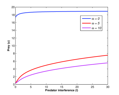
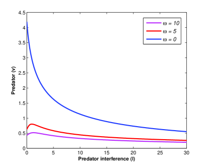
Figure 1: Impact of predator interference on (a) prey (u) and (b) predator (v) population in the presence and absence of the fear effect.

Figure 1 depicts how the fear effect reduces the population count in the presence of predator interference $(l)$. It is observed that the more they intrude on each other’s business, the more the prey count increases. And this predator interference is more effective when a certain amount of fear exists in the system. Furthermore, the counts of prey $(u)$ and predator $(v)$ species are shown in Fig. 2 for increasing the value of fear level $(\omega)$. In this case, the prey species has shown a declination for increasing value of $\omega$, which causes the reduction in predator population too. But, in this work, we have not only dealt with the fear effect but also provided a source of alternative or additional food to the predators. This figure supports the fact that the inclusion of alternative food helps to increase the prey population as they get a chance to save themselves by hiding in a safe zone, creating prey refuge while predators are busy with secondary food sources, further increasing the predator count.

Figure 2: Comparison of the components of $E^{*}$ for $\alpha=0.1,\ 0.5,\ 0.9$ while varying $\omega.$

We portray some scenarios in Fig. 3 when different system parameters are chosen as control parameters. First, it is observed that the consumption rate of predator $(a)$ contributes to the existence of the steady coexisting state [see Fig. 3(a)]. If the predator consumes the targeted prey at a very low rate to their growth, then they may not be able to survive in the system even if there is some additional food present, and a stable predator-free system occurs in such cases (e.g., stable $E_{1}$ in our case). But from this situation, if the consumption rate starts to increase, then a situation arises where both prey and predator exist in a steady state (e.g., stable coexisting equilibrium $E^{*}$). In this case, the coexisting equilibrium point switches the stability behaviour from the predator-free equilibrium $E_{1}$ through transcritical bifurcation. For the considered parameter set, this transcritical bifurcation occurs at $a=a_{[TC_{1}]}=0.115608$ [see Fig. 3(a)]. A further increment of the parameter $a$ leads to the extinction of prey species, and only predator species exist in a steady state in such cases (e.g., stable prey-free equilibrium $E_{2}$). In this case, the coexisting equilibrium point and prey-free equilibrium point exchange their stabilities through another transcritical bifurcation that occurs at $a=a_{[TC_{2}]}=0.699983$ [see Fig. 3(a)].

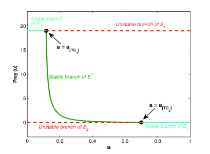
((a))

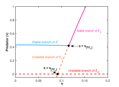
((b))

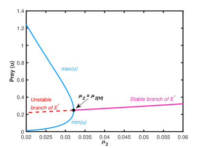
((c))

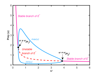
((d))

Figure 3: Change of dynamical behaviour of temporal system (2.1) with increasing (a) $c$, (b) $\eta$, (c) $\mu_{2}$ and (d) $\omega$.

We have studied the behaviour of the model when the predators go for additional food sources instead of the targeted prey, and the parameter $\eta$ is involved in signifying it. Figure 3(b) shows that if the predator detects the additional food up to a certain amount along with the prey species, then both the population exist as a steady state, but increasing the parametric value leads to a situation where the two equilibrium points $E_{2}$ and $E^{*}$ exchange their stability through a transcritical bifurcation which occurs at $\eta=\eta_{[TC_{1}]}=0.115306$. The prey-free equilibrium exists for $\eta>\eta_{[TC_{1}]}$. Also, there exists an unstable branch of $E_{2}$ when $\eta$ lies below $\eta_{[TC_{1}]}$, which ultimately emerges with the unstable trivial equilibrium $E_{0}$ through another transcritical bifurcation at $\eta=\eta_{[TC_{2}]}=0.091241$.

Now, we see how the intra-specific mortality rate of predators regulates the system dynamics, which can be controlled by the parameter $\mu_{2}$. When a predator is exposed to prey species which is inadequate in the system, then they tend to compete with each other to gain more food. This psychology remains the same even in the presence of alternative food sources. It follows in Fig. 3(c) that a certain amount of competition is needed for the coexisting equilibrium point. But both the populations start to oscillate around $E^{*}$ if $\mu_{2}$ comes below a certain threshold value through Hopf bifurcation, which occurs at $\mu_{2[H]}=0.032103$. In this case, the temporal model exhibits a supercritical Hopf bifurcation, and the first Lyapunov coefficient is $l_{1}=-0.0294$. Furthermore, it is observed that the fear term $(\omega)$ acts as a stabilizing as well as destabilizing factor in the system [see Fig. 3(d)]. Both the populations coexist and are stable for a small value of $\omega$, but an increase in the value leads to oscillation, indicating the occurrence of a supercritical Hopf bifurcation at $\omega_{[H_{1}]}=0.419521$ with the first Lyapunov coefficient $l_{1}=-0.0162$. A stable limit cycle is generated through this Hopf bifurcation and vanishes through another supercritical Hopf bifurcation at $\omega_{[H_{2}]}=3.855245$ with $l_{1}=-0.0305$. With further increased fear parameter value $\omega$, the coexisting equilibrium point remains stable [see Fig. 3(d)].

Sometimes, a predator fails to access the whole of the prey population when a prey species successfully hides in a safe zone to dodge the frequent attack of their predator. This type of scenario can be captured by the prey refuge parameter $(m)$ in the model. Figure 4(a) shows that the coexisting equilibrium point can be obtained when a certain amount of prey hides in a predator-prohibited zone, but both populations perform oscillatory behaviour if the prey refuge parameter comes below a threshold value. This situation occurs in the system through a supercritical Hopf bifurcation around the coexisting equilibrium point $E^{*}$ at $m_{[H]}=0.302811$ (the first Lyapunov coefficient is $l_{1}=-0.0389$), and stable limit cycle exists for $m<m_{[H]}$. Furthermore, the predator count has been plotted by taking the prey refuge parameter $(m)$ in Fig. 4(b) in the absence and presence of additional food sources. It is seen that the Hopf threshold shifts towards the left due to the incorporation of additional food. Therefore, the additional food expands the region where the population can coexist as the population oscillates whenever $m$ is less than the Hopf threshold [see Fig. 4(a)].

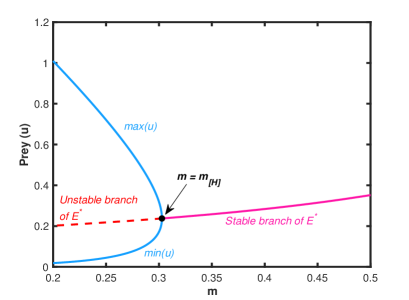
((a))

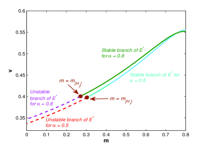
((b))

Figure 4: (a) Change of dynamical behaviour of the temporal system with increasing $m$. (b) Impact of prey refuge $(m)$ on the predator population $(v)$ in the presence of alternative food sources.

5.2 Effects of local and nonlocal interactions

We first analyze the results by incorporating local interactions in the temporal model. The focus of this work is to study the impact of fear in the presence of additional food sources. So, we choose the additional food source $\omega$ as the bifurcation parameter. Now, Turing instability is one of the main factors studied in the reaction-diffusion model, which helps to find non-homogeneous stationary patterns. For finding such Turing instability, the coexisting homogeneous steady-state has to be locally asymptotically stable. In our temporal model, there exists two Hopf bifurcation thresholds $\omega_{[H_{1}]}$ and $\omega_{[H_{2}]}$. The stable coexisting equilibrium point is found when $\omega$ lies outside these thresholds, and the system shows periodic dynamics inside these thresholds [see Fig. 3(d)]. We first focus on the temporal Hopf stable domain $\omega>\omega_{[H_{2}]}$.

For a fixed $\omega$, we obtain the Turing bifurcation threshold $d_{1[c]}$, and we plot this set of Turing bifurcation thresholds for a set of parameter values of $\omega$ in the $\omega$-$d_{1}$ plane, which is shown in Figure 5. We have plotted the Turing curve and temporal Hopf curve here, which intersect each other, and they divided the region into four sub-regions. Pure Turing domain $(R_{1})$ and homogeneous solution $(R_{4})$ lie on the right of the second Hopf curve $\omega=\omega_{[H_{2}]}$, below and above the Turing curve, respectively. On the other hand, there is another Turing domain $(R_{5})$ and homogeneous solution $(R_{6})$ exist left to the first Hopf curve $\omega=\omega_{[H_{1}]}$, below and above Turing curve respectively. The bottom region $(R_{2})$ between the two temporal Hopf curves is the Turing-Hopf domain, while the upper region $(R_{3})$ is the Hopf domain. Here, we have mainly chosen the values of $\omega$ and $d_{1}$ from $R_{1},R_{2},R_{3}$ and $R_{4}$ domains as the other two regions $R_{5}$ and $R_{6}$ will show the same dynamical nature as $R_{1}$ and $R_{4}$ respectively.

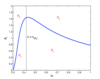
((a))

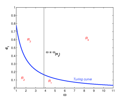
((b))

Figure 5: Temporal-Hopf, Turing bifurcation curves in the $\omega$-$d_{1}$ plane for the local model are represented by black and blue colors. The Turing domain corresponding to (a) $\omega<\omega_{[H_{1}]}$ and (b) $\omega>\omega_{[H_{2}]}$ is considered here.

To describe the Turing and non-Turing patterns for the system (3), we have chosen the spatial domain as $[-L,L]$, where $L=50$, with non-negative initial and periodic boundary conditions. To observe the dynamics, a heterogeneous perturbation is given around the coexisting homogeneous steady-state as the initial conditions. We choose small amplitude random perturbations given by $u(x_{j},0)=u^{*}+\epsilon\xi_{j}$ and $v(x_{j},0)=v^{*}+\epsilon\psi_{j}$ with $\epsilon=10^{-5}$ and $\xi_{j}$ and $\psi_{j}$ are Gaussian white noise $\delta$-correlated in space. The dynamical behaviour of the proposed spatio-temporal model is explored in Figs. 5–9. It is also noted that the nonlocal model (4) turns into a local model (3) if the range of nonlocal interaction $\delta$ tends to $0$.

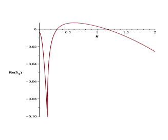
((a))

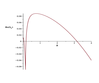
((b))

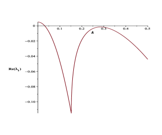
((c))

Figure 6: Plot of largest real part of eigenvalues with respect to $k$ when $(\omega,\ d_{1})$ are chosen from $R_{1},R_{2}$ and $R_{3}$ respectively. (a) Turing domain: $(\omega,\ d_{1})=(10,0.01)$, (b) Turing-Hopf domain: $(\omega,\ d_{1})=(1,0.01)$ and (c) Hopf domain: $(\omega,\ d_{1})=(2,0.38)$

For $\omega=10$ the temporal model (2.1) has the feasible interior equilibrium point $E^{*}=(0.295,0.430)$, which is stable. Also, from equation (3.3), $d_{1[c]}$ is found to be $0.0406$ when $d_{2}=10$. The real part of an eigenvalue is plotted in Fig. 6 when $d_{1}$ is chosen from Turing domain $(R_{1})$ [see Fig. 6(a)], Turing-Hopf domain $(R_{2})$ [see Fig. 6(b)] and Hopf domain $(R_{3})$ [see Fig. 6(c)]. Here, the real parts match with the cases for the temporal model for $k=0$. The oscillatory solution also occurs for the local model in the domain above the Turing curve and to the left of the temporal Hopf curve. These oscillatory solutions are homogeneous in space but periodic in time. A sample solution is plotted in Fig. 7 for $\omega=2$ and $d_{1}=0.38$.

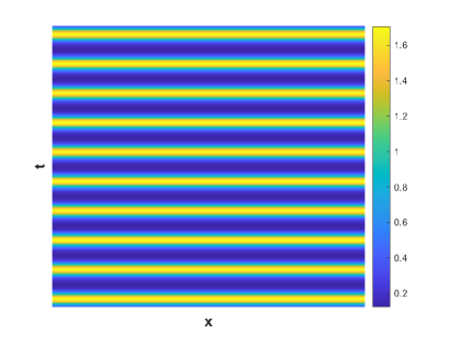
Figure 7: Contour plot of $u$ (left) and $v$ (right) for $\omega=2$ when $d_{1}=0.38$ is chosen from Hopf domain $(R_{3}$).

Some literature already states that if a specialist predator is considered in a predator-prey model, then time-dependent spatial patterns occur when the diffusion parameter is chosen from a bit inside of the temporal Hopf domain ^{61, 62}. In the Turing-Hopf domain, the Turing behaviour mainly dominates and creates stationary patterns. However, the Hopf behaviour also dominates and produces oscillatory patterns. These oscillatory solutions can be found in this domain in a small region near the Turing curve. Generally, non-homogeneous stationary patterns exist in most parts of the Turing-Hopf domain for the local model, which is depicted in Figs. 8 for $d_{1}=0.01$ and with $\omega=1$.

When $d_{1}>d_{1[c]}$ holds in the right of the temporal Hopf curve, the stationary homogeneous solution can be obtained in the stable domain $(R_{4})$. However, a decrease of the diffusion parameter $d_{1}$ makes a shift in the Turing domain $(R_{1})$, where Turing pattern solutions can be obtained for the mentioned boundary condition. In order to draw Fig. 9, let us choose $d_{1}=0.01$ from the Turing domain (see $R_{1}$ in Figure 5) when $\omega=10$. The figure depicts the stationary Turing patterns for the periodic boundary condition when parameter values are chosen from Table 1 along with $d_{2}=10$. It is observed in the figure that the amplitude of the pattern is constant in the whole domain.

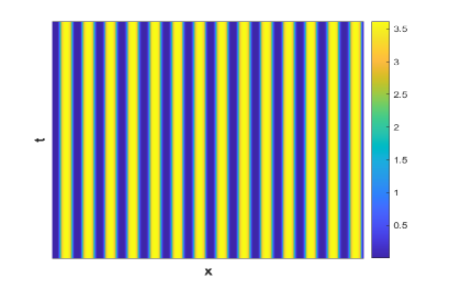
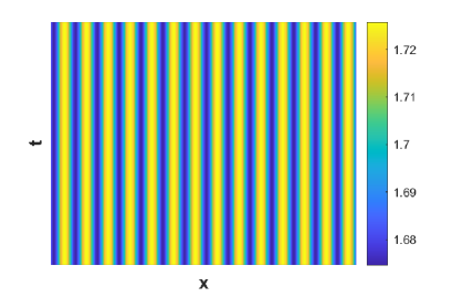
Figure 8: Contour plot of $u$ (left) and $v$ (right) for $\omega=1$ when $d_{1}(=0.01)$ is chosen from Turing-Hopf domain $(R_{2}$).

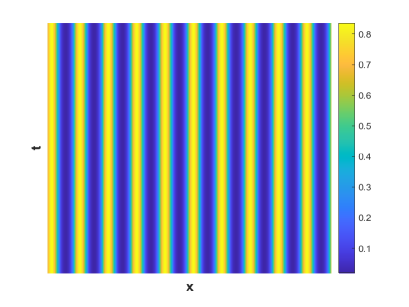
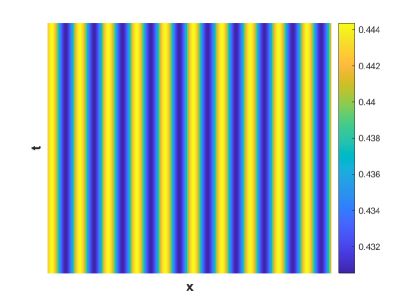
Figure 9: Contour plot of $u$ (left) and $v$ (right) for $\omega=10$ when $d_{1}(=0.01)$ is chosen from Turing domain $(R_{1}$).

Now, we study the behaviour of the nonlocal model (4) for different values of the range of nonlocal interactions $\delta$. The temporal Hopf bifurcation curve is independent of $\delta$. However, the Turing bifurcation curve depends on $\delta$. We have plotted the Turing bifurcation curves in Fig. 10 for different values of the range of nonlocal interaction. This figure shows that the Turing curve shifts upwards with an increase in the interaction range $\delta$. In this figure, we have shown the difference between the Turing curves for local and nonlocal models to emphasize the significance of nonlocal terms in the system. Furthermore, it indicates that including nonlocal interaction expands the Turing domain by increasing the chance of occurrence of stationary patterns of population.

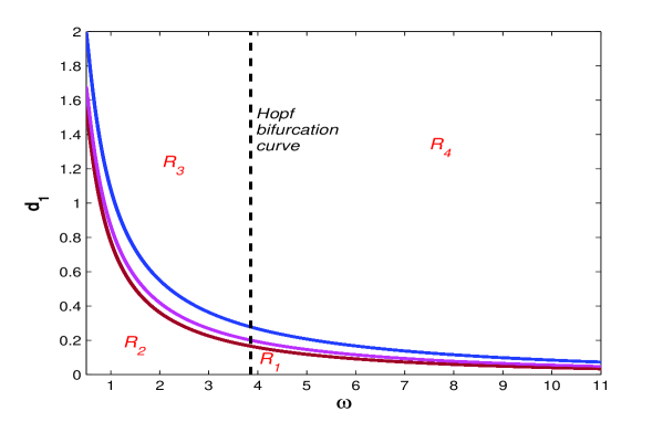
Figure 10: Temporal-Hopf curve and Turing curves for local and nonlocal models. The temporal-Hopf curve is represented by black color. The maroon color curve denotes the Turing curve for the local model, and the magenta and blue colour curves are the Turing curve for $\delta=5$ and $\delta=10$, respectively.

Now, we find the solution characteristics for the nonlocal model in each domain formed due to the intersection of the temporal Hopf and Turing curves. For a certain nonlocal interaction $\delta$, first, we consider the region to the right of the temporal Hopf curve. The pure Turing domain is the region that lies below the Turing curve. On the other hand, the stable region that lies above the Turing curve where the solutions are homogeneous under the heterogeneous perturbations around the coexisting steady-state. And, the region that lies above the Turing curve and the left of the temporal Hopf curve is called the Hopf domain. Finally, the region lying to the left of the temporal-Hopf curve and below the Turing curve is called the Turing-Hopf domain.

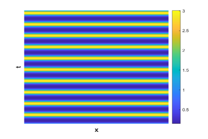
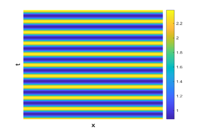
Figure 11: Contour plot of $u$ (left) and $v$ (right) for $\omega=2$ when $d_{1}(=2.5)$ is chosen from Hopf domain $(R_{3}$).

Let us first explore the solutions of the nonlocal model in the temporal Hopf unstable domain. We have chosen $\omega=2$ and $\delta=10$ and plot the corresponding solutions of the nonlocal model for $d_{1}=2.5$ and $d_{1}=0.38$ in Figs. 11 and 12, respectively. The value $d_{1}=2.5$ lies above the Turing curve, and the other values $d_{1}=0.45$ and $d_{1}=0.38$ lie in the Turing-Hopf domain away and near the Turing curve. We mainly intend to observe if the dynamical nature changes in the presence of nonlocal interaction. The oscillatory solution occurs for system (4) in the Hopf domain, which is homogeneous in space but periodic in time [see Fig. 11 for $\omega=2$ and $d_{1}=2.5$]. In the Turing-Hopf domain, the dominance of Hopf mode can be seen for the nonlocal model when the parameter values lie close to the Turing curve. Moreover, a decrease in the value of $d_{1}$ ultimately gives non-homogeneous stationary patterns for the nonlocal model, which is reflected in Figure 12.

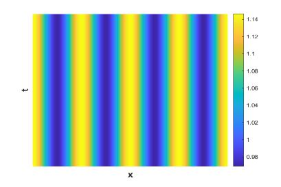
Figure 12: Contour plot of $u$ (left) and $v$ (right) for $\omega=2$ when $d_{1}(=0.38)$ is chosen from Turing-Hopf domain $(R_{2}$).

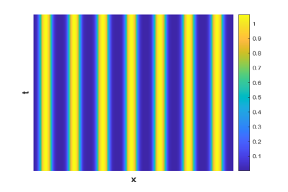
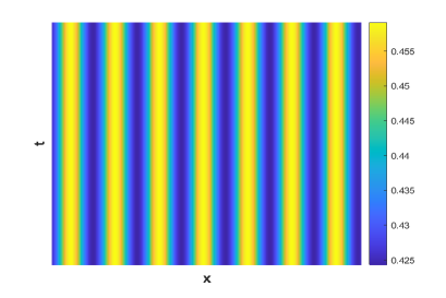
Figure 13: Contour plot of $u$ (left) and $v$ (right) for $\omega=10$ when $d_{1}(=0.01)$ is chosen from Turing domain $(R_{1}$).

For the nonlocal model, it is observed that if $d_{1}<d_{1[c]}^{T}$ holds in the right of the temporal Hopf curve, then it produces stationary Turing patterns. For instance, a Turing pattern is shown in Fig. 13 for $d_{1}=0.01$ and $\omega=10$. In addition, we have compared the behaviours of local and nonlocal models for the parameters that lie in the temporal Hopf unstable domain. For this, we choose the parameter values as $\omega=2$ and $d_{1}=0.38$. In this case, the local model shows periodic dynamics in time and homogeneous in space [see Fig. 7], but the nonlocal model shows the non-homogeneous stationary solution for $\delta=10$ [see Fig. 12]; these two types of dynamics happen due to the shifting of the Turing curve. The parameter $d_{1}$ lies in the Hopf unstable domain for the local model; however, it lies in the Turing-Hopf domain for the nonlocal model with $\delta=10$, and the Turing structure dominates the oscillation behaviour in this case. This further shows that the nonlocal interaction enhances the region of getting non-homogeneous stationary patterns, which is beneficial for their survival in the long run.

6 Conclusions

In an ecological system, prey-predator interaction is a biological phenomenon that balances the food web. The sustainability of predator species depends on their consumption process and the searching strategy for prey. This consumption process of predators depends on the resource population size, availability and the other predators’ interference. Sometimes, the growth of prey becomes affected by the frequent attack of their predator. Research reveals that only the fear of predation reduces the reproduction of song sparrow ^{4, 12}. Also, the fear of being consumed by large carnivores leads to a decline in mesocarnivores’ foraging time and strategy ¹⁰.

In this work, we have proposed a predator-prey interaction that includes psychological stress in the prey species induced by the fear of their predators. The main intention here is to elucidate the importance of this factor in the dynamic behaviour of the model, as we have assumed that the growth rate of prey is reduced due to fear of predation. Not only the fear term, but we have considered the interference in predators during the searching or handling of their prey by choosing the Beddington-DeAngelis functional response. And, as we have assumed that the predator is provided with alternative food sources, it is evident that the prey will get the scope to move towards a predator-prohibited zone by creating prey refuge, which leaves only a fraction of them for the predators for consumption. In this work, we have explored how all these factors make an impact on the dynamics of these species interaction. It is observed in the numerical simulation that the consumption rate of predators plays an important role as the system can move to a steady prey-free state or even predator-free state from a stable coexistence state while regulating this parameter [see Fig. 3(a)]. In fact, the detection of additional food $(\eta)$ also has the ability to regulate the dynamics as we have found stable interior equilibrium $(E^{*})$ from predator-free state $(E_{2})$ by decreasing the value. As the prey species creates some refugia while the predator engages with additional food, the prey species can save themselves from going extinct and steady coexistence occurs among populations [see Fig. 3(b)]. The prey refuge $(m)$ also has the regulation ability as Fig. 4 shows that when the refuge parameter lies below a threshold value, the population starts oscillating, but we get coexistence while $m$ exceeds the Hopf threshold. Not only that, but the presence of additional food increases the chances of such coexistence. Now, the fear level has been found to be a stabilizing as well as destabilizing factor in this model [see Fig. 3(d)]. Though a stable coexisting state found for a very small as well as large value of fear $(\omega<\omega_{[H_{1}]}\ \mbox{and}\ \omega>\omega_{[H_{2}]})$, but oscillation is observed when it lies within a range $\omega\in(\omega_{[H_{1}]},\ \omega_{[H_{2}]})$. It indicates that a certain amount of fear is needed in the system for the population to coexist.

In the later part of the work, it is assumed that the species are able to move in one direction described by the spatio-temporal model. The analysis reveals that the diffusion coefficient for the prey species starts to decrease with increasing fear level $(\omega)$ [see Fig. 5]. It indicates that the prey, out of the fear of being hunted, will avoid moving in the mentioned direction. In fact, the increase in $\omega$ shrinks the region of the Turing domain, reducing the chances of non-homogeneous pattern formation. As the species are not always homogeneously distributed over a domain, this shrinkage may not be proven very favourable for persistence. Further, incorporating nonlocal terms in the system shifts the Turing curve upwards, expanding the Turing domain. It means the species can be colonized with an increasing range of nonlocal interactions, and this will be beneficial for the survival of both species in the future.

Though the proposed system contains rich dynamics, it can be refined further in the future. It is assumed that the growth of prey species is affected by fear of the predator, which is one of the constraints under which the system is formulated. However, in the natural environment, the prey species may adopt different defence mechanisms as a counteraction. Therefore, considering the contribution of group defence in the prey’s growth will move the situation closer to reality. Moreover, in ecological systems, the carryover effect may take place in any prey-predator interaction where species’ past experiences and background are used to explain their present behaviour. The fear of predation is considered one of the non-lethal effects of the predator on prey, which may not affect a single generation only but can be carried over to the next generations. So, this carryover effect can be incorporated into the prey species of the model (2.1). Furthermore, the environmental stochasticity remains uncultivated in this work, which can be proposed in the system through white Gaussian noise. In the proposed model, we have considered that only a fixed portion of prey hide themselves successfully, but in the future, this model can be refined by introducing a predator-dependent refuge function. So, the system (2.1) will become even more realistic when these aspects are incorporated and analyzed.

6.1 Acknowledgements

The authors are grateful to the NSERC and the CRC Program for their support. RM is also acknowledging the support of the BERC 2022–2025 program and the Spanish Ministry of Science, Innovation and Universities through the Agencia Estatal de Investigacion (AEI) BCAM Severo Ochoa excellence accreditation SEV-2017–0718. This research was enabled in part by support provided by SHARCNET (www.sharcnet.ca) and Digital Research Alliance of Canada (www.alliancecan.ca).

6.2 Data Availability Statement

The data used to support the findings of the study are available within the article.

6.3 Conflict of Interest

This work does not have any conflict of interest.

6.4 Bibliography

References

- 1 Lima SL, Dill LM. Behavioral decisions made under the risk of predation: a review and prospectus. Canadian journal of zoology 1990; 68(4): 619–640.
- 2 Pangle KL, Peacor SD, Johannsson OE. Large nonlethal effects of an invasive invertebrate predator on zooplankton population growth rate. Ecology 2007; 88(2): 402–412.
- 3 Preisser EL, Bolnick DI, Benard MF. Scared to death? The effects of intimidation and consumption in predator–prey interactions. Ecology 2005; 86(2): 501–509.
- 4 Zanette LY, White AF, Allen MC, Clinchy M. Perceived predation risk reduces the number of offspring songbirds produce per year. Science 2011; 334(6061): 1398–1401.
- 5 Ripple WJ, Beschta RL. Wolves and the ecology of fear: can predation risk structure ecosystems?. BioScience 2004; 54(8): 755–766.
- 6 Wirsing AJ, Heithaus MR, Dill LM. Living on the edge: dugongs prefer to forage in microhabitats that allow escape from rather than avoidance of predators. Animal Behaviour 2007; 74(1): 93–101.
- 7 Altendorf KB, Laundré JW, López González CA, Brown JS. Assessing effects of predation risk on foraging behavior of mule deer. Journal of mammalogy 2001; 82(2): 430–439.
- 8 Creel S, Christianson D, Liley S, Winnie Jr JA. Predation risk affects reproductive physiology and demography of elk. Science 2007; 315(5814): 960–960.
- 9 Gallagher AJ, Lawrence MJ, Jain-Schlaepfer SM, Wilson AD, Cooke SJ. Avian predators transmit fear along the air–water interface influencing prey and their parental care. Canadian Journal of Zoology 2016; 94(12): 863–870.
- 10 Suraci JP, Clinchy M, Dill LM, Roberts D, Zanette LY. Fear of large carnivores causes a trophic cascade. Nature communications 2016; 7(1): 10698.
- 11 Wang X, Zanette L, Zou X. Modelling the fear effect in predator–prey interactions. Journal of mathematical biology 2016; 73(5): 1179–1204.
- 12 Allen MC, Clinchy M, Zanette LY. Fear of predators in free-living wildlife reduces population growth over generations. Proceedings of the National Academy of Sciences 2022; 119(7): e2112404119.
- 13 Hua F, Sieving KE, Fletcher Jr RJ, Wright CA. Increased perception of predation risk to adults and offspring alters avian reproductive strategy and performance. Behavioral Ecology 2014; 25(3): 509–519.
- 14 Wirsing AJ, Ripple WJ. A comparison of shark and wolf research reveals similar behavioral responses by prey. Frontiers in Ecology and the Environment 2011; 9(6): 335–341.
- 15 Sheriff MJ, Krebs CJ, Boonstra R. The sensitive hare: sublethal effects of predator stress on reproduction in snowshoe hares. Journal of Animal Ecology 2009; 78(6): 1249–1258.
- 16 Laundré JW, Hernández L, Altendorf KB. Wolves, elk, and bison: reestablishing the" landscape of fear" in Yellowstone National Park, USA. Canadian Journal of Zoology 2001; 79(8): 1401–1409.
- 17 Wootton RJ. Ecology of teleost fishes. 1. Springer Science & Business Media . 2012.
- 18 Thirthar AA, Majeed SJ, Alqudah MA, Panja P, Abdeljawad T. Fear effect in a predator-prey model with additional food, prey refuge and harvesting on super predator. Chaos, Solitons & Fractals 2022; 159: 112091.
- 19 Zhang N, Kao Y, Xie B. Impact of fear effect and prey refuge on a fractional order prey–predator system with Beddington–DeAngelis functional response. Chaos: An Interdisciplinary Journal of Nonlinear Science 2022; 32(4).
- 20 Xie B, Zhang N. Influence of fear effect on a Holling type III prey-predator system with the prey refuge. AIMS Mathematics 2022; 7(2): 1811–1830.
- 21 Saha S, Samanta G. Analysis of a tritrophic food chain model with fear effect incorporating prey refuge. Filomat 2021; 35(15): 4971–4999.
- 22 Zhang H, Cai Y, Fu S, Wang W. Impact of the fear effect in a prey-predator model incorporating a prey refuge. Applied Mathematics and Computation 2019; 356: 328-337.
- 23 Holling CS. The components of predation as revealed by a study of small-mammal predation of the European Pine Sawfly1. The canadian entomologist 1959; 91(5): 293–320.
- 24 Beddington JR. Mutual interference between parasites or predators and its effect on searching efficiency. The Journal of Animal Ecology 1975: 331–340.
- 25 DeAngelis DL, Goldstein R, O’Neill RV. A model for tropic interaction. Ecology 1975; 56(4): 881–892.
- 26 Huisman G, De Boer RJ. A formal derivation of the “Beddington” functional response. Journal of theoretical biology 1997; 185(3): 389–400.
- 27 Saha S, Maiti A, Samanta G. A Michaelis–Menten predator–prey model with strong Allee effect and disease in prey incorporating prey refuge. International Journal of Bifurcation and Chaos 2018; 28(06): 1850073.
- 28 Saha S, Samanta G. Analysis of a predator–prey model with herd behavior and disease in prey incorporating prey refuge. International Journal of Biomathematics 2019; 12(01): 1950007.
- 29 Yue Q. Dynamics of a modified Leslie–Gower predator–prey model with Holling-type II schemes and a prey refuge. SpringerPlus 2016; 5(1): 1–12.
- 30 Ghosh J, Sahoo B, Poria S. Prey-predator dynamics with prey refuge providing additional food to predator. Chaos, Solitons & Fractals 2017; 96: 110–119.
- 31 Wang J, Cai Y, Fu S, Wang W. The effect of the fear factor on the dynamics of a predator-prey model incorporating the prey refuge. Chaos: An Interdisciplinary Journal of Nonlinear Science 2019; 29(8).
- 32 Lambert MS. Control of Norway rats in the agricultural environment: alternatives to rodenticide use. PhD thesis. University of Leicester, https://hdl.handle.net/2381/27745; 2003.
- 33 Lv Y, Yuan R, Pei Y. A prey-predator model with harvesting for fishery resource with reserve area. Applied Mathematical Modelling 2013; 37(5): 3048–3062.
- 34 Hoy M. Almonds (California). Spider mites: their biology, natural enemies and control, World Crop Pests 1985; 1: 229–310.
- 35 Srinivasu P, Prasad B, Venkatesulu M. Biological control through provision of additional food to predators: a theoretical study. Theoretical Population Biology 2007; 72(1): 111–120.
- 36 Chakraborty K, Das SS. Biological conservation of a prey–predator system incorporating constant prey refuge through provision of alternative food to predators: a theoretical study. Acta biotheoretica 2014; 62: 183–205.
- 37 Group MW, others . Diversionary feeding of hen harriers on grouse moors a practical guide. Scottish Natural Heritage 1999.
- 38 Crawley MJ. Plant ecology. John Wiley & Sons . 2009.
- 39 Huxel GR, McCann K, Polis GA. Effects of partitioning allochthonous and autochthonous resources on food web stability. Ecological Research 2002; 17: 419–432.
- 40 Srinivasu P, Prasad B. Role of quantity of additional food to predators as a control in predator–prey systems with relevance to pest management and biological conservation. Bulletin of mathematical biology 2011; 73(10): 2249–2276.
- 41 Das A, Samanta G. A prey–predator model with refuge for prey and additional food for predator in a fluctuating environment. Physica A: Statistical Mechanics and its Applications 2020; 538: 122844.
- 42 Zhang JF, Li WT, Yan XP. Hopf bifurcation and Turing instability in spatial homogeneous and inhomogeneous predator–prey models. Applied Mathematics and Computation 2011; 218(5): 1883-1893.
- 43 Banerjee M, Abbas S. Existence and non-existence of spatial patterns in a ratio-dependent predator–prey model. Ecological Complexity 2015; 21: 199-214.
- 44 Guin LN, Haque M, Mandal PK. The spatial patterns through diffusion-driven instability in a predator–prey model. Applied Mathematical Modelling 2012; 36(5): 1825-1841.
- 45 Wilson RE, Capasso V. Analysis of a Reaction-Diffusion System Modeling Man–Environment–Man Epidemics. SIAM Journal on Applied Mathematics 1997; 57(2): 327-346.
- 46 Fussmann GF, Ellner SP, Shertzer KW, Hairston Jr NG. Crossing the Hopf bifurcation in a live predator-prey system. Science 2000; 290(5495): 1358–1360.
- 47 Wang W, Liu QX, Jin Z. Spatiotemporal complexity of a ratio-dependent predator-prey system. Phys. Rev. E 2007; 75: 051913.
- 48 Banerjee M, Volpert V. Prey-predator model with a nonlocal consumption of prey. Chaos: An Interdisciplinary Journal of Nonlinear Science 2016; 26(8).
- 49 Banerjee M, Zhang L. Stabilizing role of nonlocal interaction on spatio-temporal pattern formation. Mathematical Modelling of Natural Phenomena 2016; 11(5): 103–118.
- 50 Banerjee M, Volpert V. Spatio-temporal pattern formation in Rosenzweig–MacArthur model: Effect of nonlocal interactions. Ecological Complexity 2017; 30: 2-10.
- 51 Bayliss A, Volpert V. Complex predator invasion waves in a Holling–Tanner model with nonlocal prey interaction. Physica D: Nonlinear Phenomena 2017; 346: 37-58.
- 52 Embar K, Raveh A, Hoffmann I, Kotler BP. Predator facilitation or interference: a game of vipers and owls. Oecologia 2014; 174: 1301–1309.
- 53 Skalski GT, Gilliam JF. Functional responses with predator interference: viable alternatives to the Holling type II model. Ecology 2001; 82(11): 3083–3092.
- 54 Zhang S, Chen L. A study of predator–prey models with the Beddington–DeAnglis functional response and impulsive effect. Chaos, Solitons & Fractals 2006; 27(1): 237–248.
- 55 Pal S, Majhi S, Mandal S, Pal N. Role of fear in a predator–prey model with Beddington–DeAngelis functional response. Zeitschrift für Naturforschung A 2019; 74(7): 581–595.
- 56 Cantrell RS, Cosner C. Spatial ecology via reaction-diffusion equations. John Wiley & Sons . 2004.
- 57 Du NH, Trung TT. On the dynamics of predator-prey systems with Beddington-DeAngelis functional response. Asian-European Journal of Mathematics 2011; 4(01): 35–48.
- 58 Hale JK. Analytic Theory of Differential Equations . 1977.
- 59 Perko L. Differential equations and dynamical systems. 7. Springer Science & Business Media . 2013.
- 60 Pal S, Banerjee M, Ghorai S. Effects of boundary conditions on pattern formation in a nonlocal prey–predator model. Applied Mathematical Modelling 2020; 79: 809–823.
- 61 Petrovskii SV, Malchow H. Wave of chaos: new mechanism of pattern formation in spatio-temporal population dynamics. Theoretical population biology 2001; 59(2): 157–174.
- 62 Petrovskii S, Li BL, Malchow H. Quantification of the spatial aspect of chaotic dynamics in biological and chemical systems. Bulletin of mathematical biology 2003; 65(3): 425–446.