Dislocation dynamics in Ni-based superalloys: Parameterising dislocation trajectories from atomistic simulations

Abstract

Nickel-based superalloys are important materials for high temperature applications. Nanoscale precipitates in their microstructure hinder dislocation motion, which results in an extraordinary strengthening effect at elevated temperatures. In the present work, we study the deformation behaviour of these materials using molecular dynamics (MD) simulations using classical effective potentials. In our simulations, we observed the movement of an $\frac{a}{2}\langle 110\rangle\{111\}$ edge dislocation under shear in pure Ni, which is used to model the Ni solid solution matrix, and extracted the locations of the dislocations. We show how a Differential Evolution Monte Carlo (DE-MC) analysis is an effective way to find the parameters of an equation of motion for the dislocation lines with quantified uncertainties. The parameters of interest were the effective mass, drag coefficient, and force experienced by the dislocation. The marginal parameter and joint posterior distributions were estimated from the accepted samples produced by the DE-MC algorithm. The equation of motion and parameter distributions were used to predict the dislocation positions and velocities at the simulation timesteps, and the mean fit was found to match the MD trajectories with an RMSE of $0.13\text{\,}\mathrm{nm}$. We also discuss how the selected model can be extended to account for the presence of multiple dislocations as well as dislocation-precipitate interactions. This work serves as the first step towards building a predictive surrogate model that describes the deformation behaviour of Ni-based superalloys.

1 Introduction

Ni-based superalloys are important materials that are widely used in high-temperature applications. Precipitation strengthening provided by $\gamma^{\prime}$ (Ni₃Al) precipitates, which hinder dislocation motion, plays a major role in providing the extraordinary strength exhibited by these alloys. The ordered L1₂ $\gamma^{\prime}$ phase is precipitated out of the face-centered cubic (FCC) $\gamma$ matrix, which is a Ni solid solution phase.

Understanding the dynamics of dislocations in these alloys is central to studying their deformation behaviour. Here, we present a methodology to parameterise the motion of dislocations in the $\gamma$ matrix based on the work of Bitzek et al.  [1, 2, 3]. Pure FCC Ni is used as a model system to represent the $\gamma$ phase in these alloys. The effect of the $\gamma^{\prime}$ precipitates on the dislocation motion is considered in a future work. In FCC metals, the primary dislocations of interest are the $\frac{a}{2}\langle 110\rangle\{111\}$ edge dislocations, which are perfect dislocations. It is energetically favorable for these dislocations to dissociate into two partial dislocations with a stacking fault (SF) in between:

$$\frac{1}{2}[\bar{1}10]\rightarrow\frac{1}{6}[\bar{2}11]+SF+\frac{1}{6}[\bar{1}2\bar{1}]$$ (1)

Previously, Bitzek et al. [1, 2, 3] postulated an equation of motion (2) of the form

$$m\frac{d^{2}x}{dt^{2}}+B\frac{dx}{dt}=F,$$ (2)

and identified the parameters through Least Squares (LS) fitting to dislocation trajectories generated using molecular dynamics (MD). In equation (2), $m$ is the effective mass of the dislocation and determines the dislocation’s effective inertia; $B$ is the drag coefficient and describes the lattice resistance to dislocation motion; and $F$ is the force experienced by the dislocation. $F$ is assumed to decompose as $F=F_{a}+F_{i}$, where $F_{a}$ is the Peach-Koehler force and $F_{i}$ is the force that results from dislocation interactions with defects and lattice resistance. It should be noted that at dislocation velocities comparable with the sound speed in the material, the effective dislocation mass $m$ has a velocity-dependent component such that $m_{\text{eff}}=m_{0}+f(v)$, where $m_{0}$ is the rest mass of the dislocation and $f(v)$ is a function of the dislocation velocity $v$. In the following, the velocity dependence of the mass is ignored and our analysis is limited to slow-moving dislocations under low applied shear stresses.

Here, rather than using LS, we use Differential Evolution Monte Carlo (DE-MC) as a sampling approach to fit the model parameters in (2) to edge dislocation trajectories in pure Ni. DE-MC is an adaptive Monte Carlo technique with the advantage of fast convergence in cases where parameters are highly correlated, which is the case for the current model. In conventional DE-MC, several Markov chains are run in parallel and the current state of a given chain, $\boldsymbol{\theta}_{i}$, which corresponds to a parameter vector, is updated by generating a proposal, $\boldsymbol{\theta}_{p}$, which depends on the states of two randomly selected chains from the pool of remaining chains, $R_{1}$ and $R_{2}$:

$$\boldsymbol{\theta}_{p}=\boldsymbol{\theta}_{i}+\gamma(\boldsymbol{\theta}_{R_{1}}-\boldsymbol{\theta}_{R_{2}})+\mathbf{e},$$ (3)

where $\gamma$ is a scaling factor and $\mathbf{e}$ is a random vector drawn from a narrow, symmetric distribution. A proposal, $\boldsymbol{\theta}_{p}$, is accepted with a probability min(1, $r$), where $r=\pi(\boldsymbol{\theta}_{p})/\pi(\boldsymbol{\theta}_{i})$ and $\pi(.)$ is the probability density function (pdf) of the $d$-dimensional target distribution to be sampled. If past states of chains are considered for the update, this is denoted as DE-MC_Z. DE-MC_ZS (used here), uses both past states as well as a snooker update, where a given chain is updated according to the following:

$$\boldsymbol{\theta}_{p}=\boldsymbol{\theta}_{i}+\gamma(\mathbf{z}_{P1}-\mathbf{z}_{P2})$$ (4)

where $\mathbf{z}_{P1}$ and $\mathbf{z}_{P2}$ are the orthogonal projections of $\boldsymbol{\theta}_{R1}$ and $\boldsymbol{\theta}_{R2}$ from (3) on to the line $\boldsymbol{\theta}_{i}-\mathbf{z}$, where $\mathbf{z}$ is the state of another chain. The acceptance ratio in this case then becomes:

$$r=\frac{\pi(\boldsymbol{\theta}_{p})||\boldsymbol{\theta}_{p}-\mathbf{z}||^{d-1}}{\pi(\boldsymbol{\theta}_{i})||\boldsymbol{\theta}_{i}-\mathbf{z}||^{d-1}}$$ (5)

Both the DE-MC_Z and DE-MC_ZS algorithms reduce the number of chains needed for the DE-MC sampling to converge. For more information on the development of the DE-MC algorithm and the more recent snooker update, the reader is referred to Refs. [4] and [5].

Parameterising the motion of dislocations in this way is useful, as the resulting parameters can be used as inputs to larger lengthscale approaches (e.g. discrete dislocation dynamics (DDD) [1]), which are needed to capture the complex nature of the deformation behavior of metals. Moreover, there are several advantages to using sampling to fit the model in (2) to dislocation position data. Using sampling, we not only get parameter values but also their probability distributions. This means that we are able to select the most probable parameter values as well as obtaining parameter distributions that allow us to quantify the uncertainty in the model predictions, namely the dislocation positions and velocities.

2 Methods

2.1 Molecular dynamics simulations of edge dislocations

Using the LAMMPS package [6], Molecular Dynamics (MD) simulations of $\frac{a}{2}\langle 110\rangle\{111\}$ edge dislocations in pure Ni were carried out using the Mishin [7] embedded atom method (EAM) potential. The lattice constant, $a_{0}$, used for Ni was $0.352\text{\,}\mathrm{nm}$ and the MD timestep was $0.001\text{\,}\mathrm{ps}$. To create the edge dislocation, a single [110] plane was removed from a pure Ni block, followed by relaxing the atom positions to get the correct dislocation core structure. This leads to the dissociation of the dislocation into two partial dislocations as is expected for FCC materials. The dislocation was inserted in a box with dimensions $L_{x}=$38\text{\,}\mathrm{nm}$$, $L_{y}=$17\text{\,}\mathrm{nm}$$, and $L_{z}=$30\text{\,}\mathrm{nm}$$, which was selected after testing a range of box sizes to avoid finite size effects. Periodic boundary conditions (PBCs) were applied in the $[1\bar{1}0]$ direction (the glide direction of the dislocation) as well as the $[11\bar{2}]$ direction (along the dislocation line) such that an infinitely long dislocation is obtained. A schematic of the simulation box used is shown in Fig. 1.

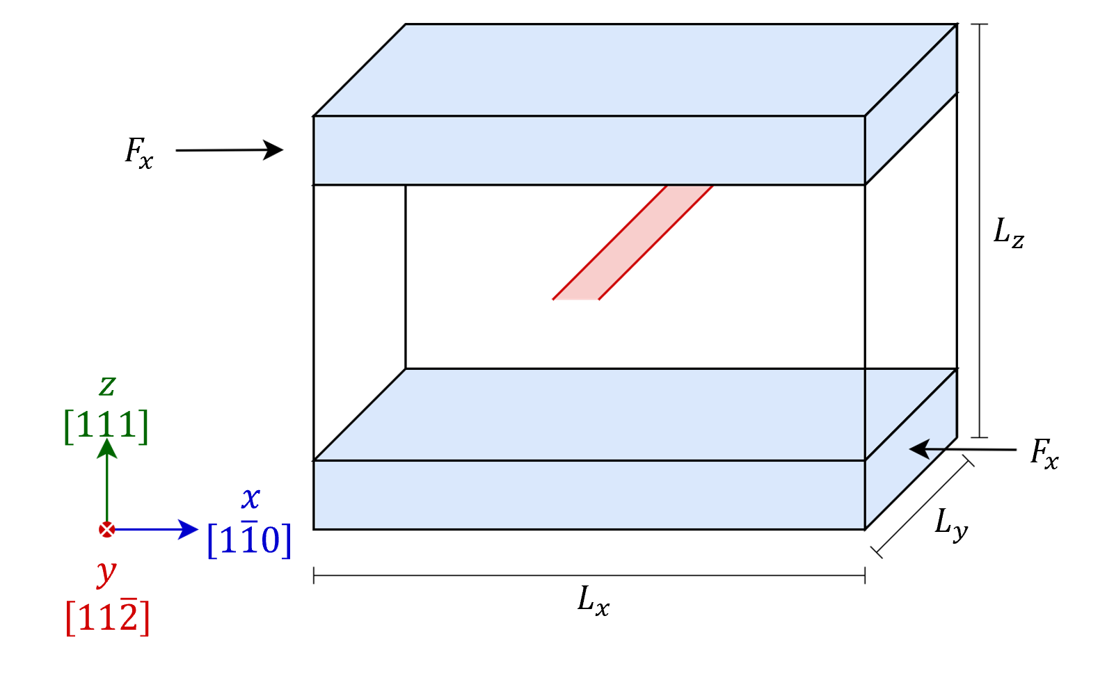
Figure 1: Schematic of the simulation box used. The dissociated edge dislocations is shown as the two $\frac{a}{6}<112>$ partial dislocations in red with the stacking fault in between. Periodic boundaries are applied in the $x$ and $y$ directions. The cell is non-periodic in $z$. To shear the cell, a force $F_{x}$ is applied to the atoms in the top and bottom layers of cell shaded in blue.

To simulate the dynamics of the edge dislocation, the simulation box was deformed under a shear stress, $\sigma=$10\text{\,}\mathrm{MPa}$$, by applying a constant force $F_{x}=\pm\sigma A/N$ to the atoms in the top and bottom layers of the box, where $A=L_{x}\times L_{y}$ is the cross-sectional area of the simulation box in the $xy$-plane and $N$ is the number of atoms in each layer. To reduce the effects of the initial stress wave, the simulation box was prestrained by slightly displacing the atoms in the top and bottom halves of the box [8] followed by another energy minimization. The simulations were carried out in the canonical ensemble at $300\text{\,}\mathrm{K}$ using a Nosé-Hoover thermostat [9], where the system was allowed to equilibrate prior to applying the shear force.

The OVITO Dislocation Analysis Tool (DXA) [10] was used to extract the positions of the partial dislocations from the $100\text{\,}\mathrm{ps}$ MD trajectories. The positions of the two partial dislocations were averaged to study the dynamics of the perfect dislocation. On analysing the dislocation trajectories, we found that it takes several picoseconds for the correct strain field to develop in the simulation cell. Accordingly, the beginning portions of the trajectories were discarded, and the equation of motion given in equation (2) was fit to the remaining data points as discussed in the following sections.

2.2 Model fitting using DE-MC

After obtaining the dislocation positions as a function of time, the parameters $m$, $B$ and $F$ were calculated by fitting equation (2) to the position data using DE-MC. Prior to fitting, some manipulation of equation (2) was necessary; dividing through by $m$, we obtain

$$\frac{d^{2}x}{dt^{2}}+\frac{B}{m}\frac{dx}{dt}=\frac{F}{m}$$ (6)

The choice to scale the coefficients in this way was made to avoid the infinite family of $m$, $B$ and $F$ that generate identical solutions to equation (2). In order to recover the full set of parameters, at low velocities relative to the speed of sound, the drag coefficient, $B$, can be calculated from

$$B=\frac{\tau b}{v_{t}}$$ (7)

for a given applied shear stress $\tau$, Burgers vector $b$, and the terminal (equilibrium) dislocation velocity $v_{t}$. The value of $B$ calculated in this way can then used with the fitted $\frac{B}{m}$ and $\frac{F}{m}$ to calculate the corresponding values of $m$ and $F$.

Equation (6) was then put in a non-dimensional form:

$$\frac{d^{2}\tilde{x}}{d\tilde{t}^{2}}+c_{0}\frac{d\tilde{x}}{d\tilde{t}}=c_{1}$$ (8)

using the expressions for the non-dimensional positions $\tilde{x}$, and time $\tilde{t}$,

$$\tilde{x}=\frac{x-x_{0}}{x_{s}},\hskip 10.00002pt\tilde{t}=\frac{t}{t_{s}},\hskip 10.00002pt\\$$ (9)

where $x_{0}$ is the initial position of the dislocation, $x_{s}$ is the total distance the dislocation has moved in the simulation and $t_{s}$ is the total simulation time. The resulting non-dimensional parameters $c_{0}$ and $c_{1}$ are related to the ratios $\frac{B}{m}$ and $\frac{F}{m}$, respectively, by the following expressions:

$$c_{0}=\frac{Bt_{s}}{m},\hskip 10.00002ptc_{1}=\frac{Ft_{s}^{2}}{mx_{s}}.\hskip 10.00002pt$$ (10)

Finally, to ensure the non-dimensional parameters are positive, $c_{0}$ and $c_{1}$ are represented as exponentials of scalar parameters $\tilde{c}_{0}$ and $\tilde{c}_{1}$, giving

$$\frac{d^{2}\tilde{x}}{d\tilde{t}^{2}}+e^{\tilde{c}_{0}}\frac{d\tilde{x}}{d\tilde{t}}=e^{\tilde{c}_{1}},$$ (11)

with $\tilde{c}_{i}=\ln c_{i}$.

DE-MC with 12 chains was then used to fit $\tilde{c}_{0}$ and $\tilde{c}_{1}$ in equation (11) to the position vs. time data obtained from MD simulations of edge dislocations in pure Ni. The $\text{MC}^{3}$ code [11] was used for the implementation of the DE-MC algorithm (with the snooker updater, referred to as DE-MC_z) within a Bayesian framework. Given the MD dislocation position data denoted by $\mathbf{y}=(y_{1},\ldots,y_{n})$, the target distribution is the joint probability density function (PDF), $p(\mathbf{y}|\mathbf{\theta})$, where $y_{i}$ is the average position of the perfect dislocation at time, $t_{i}$, and $\mathbf{\theta}$ is the vector of model parameters, $\mathbf{\theta}=(\theta_{0}\,,\theta_{1})$. Assuming a Gaussian noise $\epsilon\sim\mathcal{N}(0,\sigma^{2})$, the data can be modeled as the sum of the model predictions, $f_{i}(t_{i};\theta)$, and the noise, $\epsilon_{i}$:

$$y_{i}=f_{i}(t_{i};\theta)+\epsilon_{i}$$ (12)

given by equation (12). The PDF $p(\mathbf{y}|\mathbf{\theta})$, is then proportional to the product of a Gaussian likelihood and the prior:

$$p(\mathbf{y}|\mathbf{\theta}) =\mathcal{N}\left(\mathbf{y}|f(\mathbf{t};\theta),\sigma^{2}\mathbf{I}\right)\,\times\,\text{Prior}$$ (13)

$$=\prod\limits_{i}\mathcal{N}\left(y_{i}|f(t_{i};\theta),\sigma\right)\,\times\,\text{Prior}$$

$$=\prod\limits_{i}\left[\frac{1}{\sigma\sqrt{2\pi}}\,\text{exp}\left(\frac{f(t_{i};\theta)-y_{i}}{2\sigma}\right)^{2}\right]\times\text{Prior}$$

In the $\text{MC}^{3}$ code [11], the logarithm of the posterior distribution, $\log p(\mathbf{y}|\mathbf{\theta})$, is used. Ignoring the constant terms, $\log p(\mathbf{y}|\mathbf{\theta})$ is given by:

$$\log p(\mathbf{y}|\mathbf{\theta})=\sum\limits_{i}\left(\frac{f(t_{i};\theta)-y_{i}}{2\sigma}\right)^{2}+\log\text{Prior}$$ (14)

For the results presented here, a prior distribution $\mathcal{N}(0.0,2.0^{2})$ was used for each of the parameters. The noise, $\epsilon$, is assumed to follow a distribution $\mathcal{N}(0.0,0.025^{2})$, and is the same across all data points, corresponding to an assumption of homoskedastic noise. The accepted samples were used to estimate the posterior distribution by calculating the mean of each parameter and the covariance between them. A burn-in of $10^{5}$ samples were discarded and were not included in the analysis. To evaluate the convergence of the sampling, trace plots as well as convergence plots of the parameter means and standard deviations with the number of DE-MC generations were used.

To quantify the uncertainty in the dislocation positions predicted by the model, samples were drawn from the estimated posterior distribution and used to evaluate the model at different time values. Accordingly, a distribution was obtained for the dislocation position at every time $t_{i}$. The mean fit was obtained as the mean of each distribution at time $t_{i}$, and the uncertainty in the positions was calculated as $\pm 2$ standard deviations. The root mean squared error (RMSE) of the fit was calculated by comparing the mean predicted positions to the actual positions obtained using MD.

The marginal posterior distributions of the fitted parameters are also reported. When doing the sampling using DE-MC, if $\mathbf{\theta}=(\theta_{0}\,,\theta_{1})$ is an accepted sample, then $c_{i}=e^{\theta_{i}}$ and $\ln c_{i}=\theta_{i}$. Accordingly, in our analysis, the marginal posterior distributions presented are for $\ln c_{i}$, since these are normally distributed and are convenient to work with. However, when showing the model fit to the position data, the dimensional forms $m$, $B$, and $F$ are recovered and the mean values are reported for these quantities.

3 Results and discussion

3.1 Marginal parameter and joint posterior distributions

Figure 2 shows the histograms of the accepted samples for $\ln c_{0}$ and $\ln c_{1}$, normalized to give the probability density. Using the accepted samples, the mean and standard deviation of each parameter were calculated, and the parameters were found to follow $\ln c_{0}\sim\mathcal{N}(1.87,0.29^{2})$ and $\ln c_{1}\sim\mathcal{N}(2.06,0.22^{2})$. These are the marginal parameter posterior distributions and are also shown in Fig. 2 for each parameter and fit the histograms well. The joint posterior distribution is given by the multivariate normal distribution, $\mathcal{N}(\boldsymbol{\mu},\boldsymbol{\Sigma})$, with mean vector, $\boldsymbol{\mu}$, and covariance matrix, $\boldsymbol{\Sigma}$, which was also calculated from the accepted samples and are given as:

$$\mathcal{N}(\boldsymbol{\mu},\,\boldsymbol{\Sigma}),\,\hskip 10.00002pt\boldsymbol{\mu}=\begin{pmatrix}1.87\\ 2.06\end{pmatrix},\,\hskip 10.00002pt\boldsymbol{\Sigma}=\begin{pmatrix}0.08&0.06\\ 0.06&0.05\end{pmatrix}$$ (15)

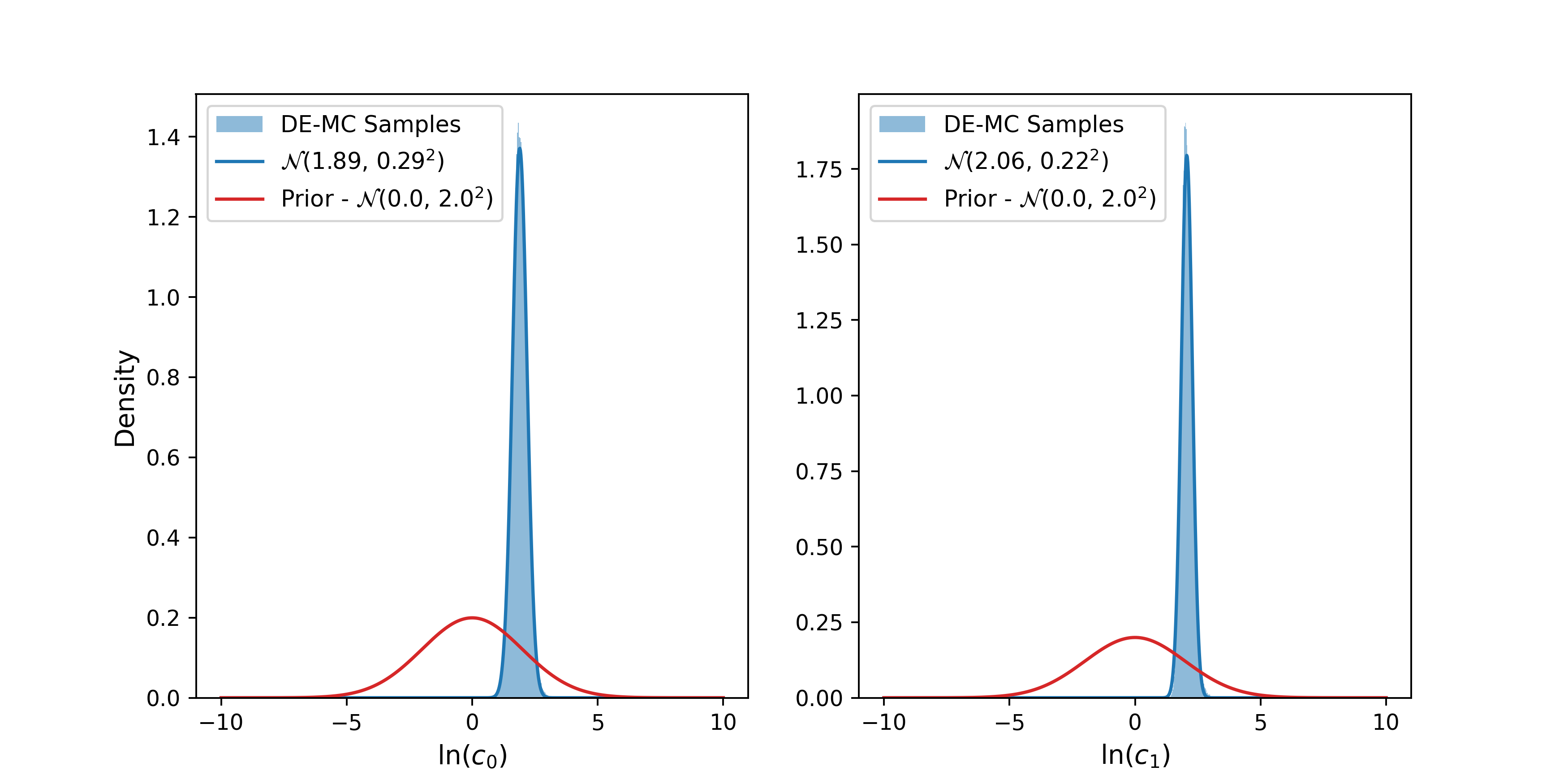
Figure 2: Marginal posterior distributions of $\ln c_{0}$ and $\ln c_{1}$ estimated from the accepted samples from the DE-MC sampling. The parameter prior distributions are shown in red.

The $\mathcal{N}(0.0,2.0^{2})$ prior distribution used for each parameter is also shown and it can be seen that the marginal parameter posterior distributions are contained within the prior. Choosing the prior distribution in this way assumes that the parameters are independent, however, it can be seen from the estimated posterior covariance matrix, $\boldsymbol{\Sigma}$, and the pair plots in Fig. 3 that the DE-MC sampling captures the covariance of the model parameters, which are highly correlated. This parameter correlation can explain why the sampling failed to converge when attempting to carry out the fitting using traditional MCMC. However, the trace plots shown in Fig.  4 and calculating the parameter means and standard deviations as a function of the number of DE-MC generations in Fig. 5 shows that the sampling is well-converged for both parameters. Moreover, the sampling acceptance rate is $>30\%$, which is within the expected range for a multivariate normal target with dimension $d=2$ [4].

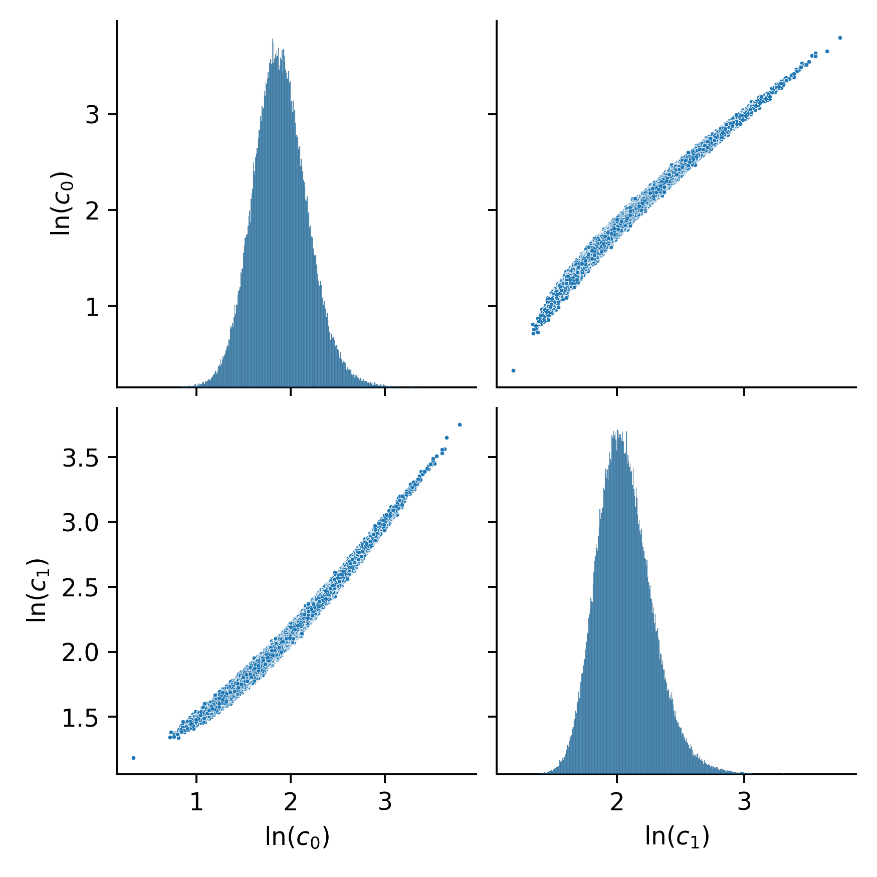
Figure 3: Pair plot showing the correlation between $\ln c_{0}$ and $\ln c_{1}$.

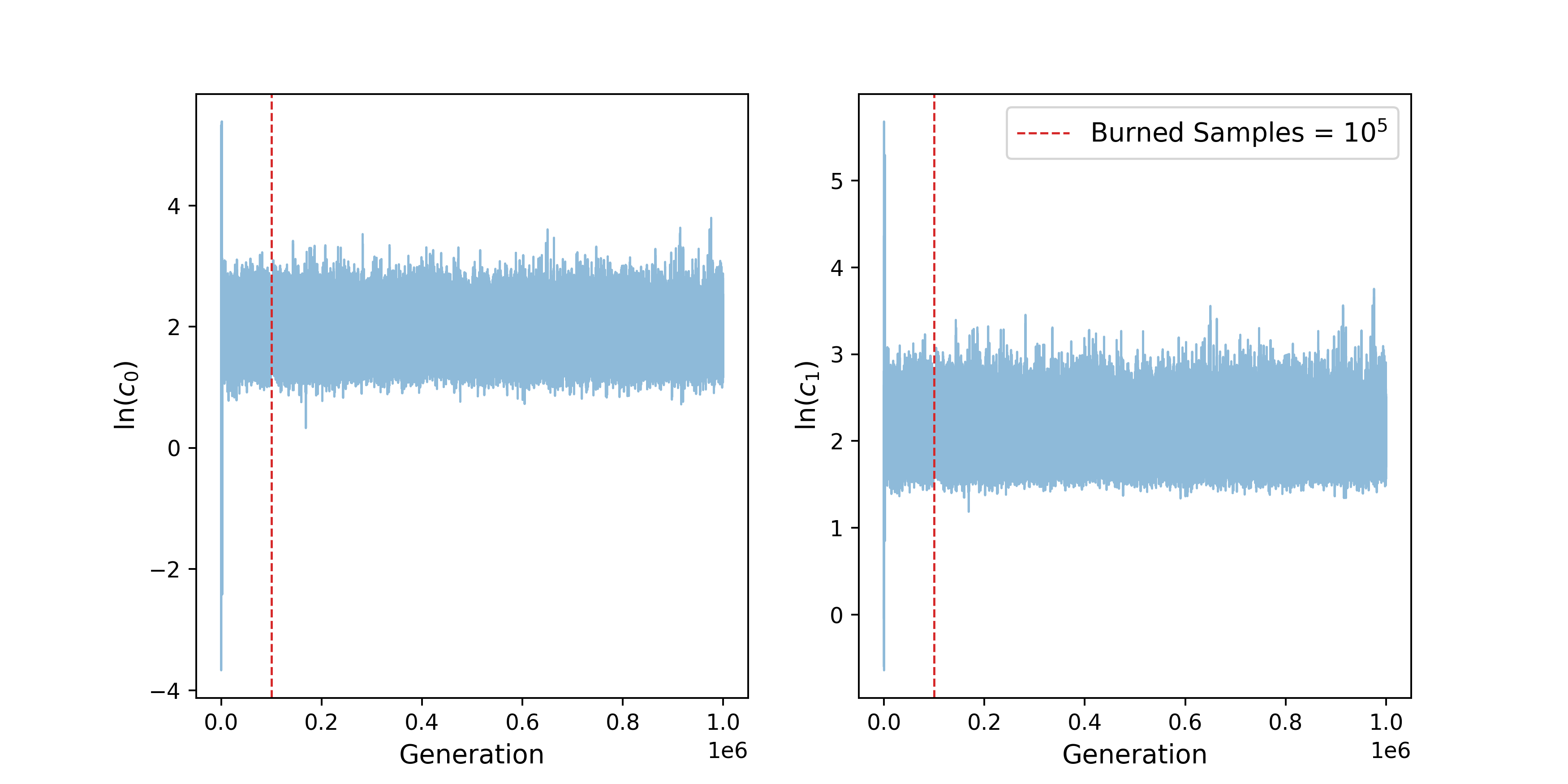
Figure 4: Trace plot showing the accepted samples for $\ln c_{0}$ and $\ln c_{1}$ with the DE-MC generation.

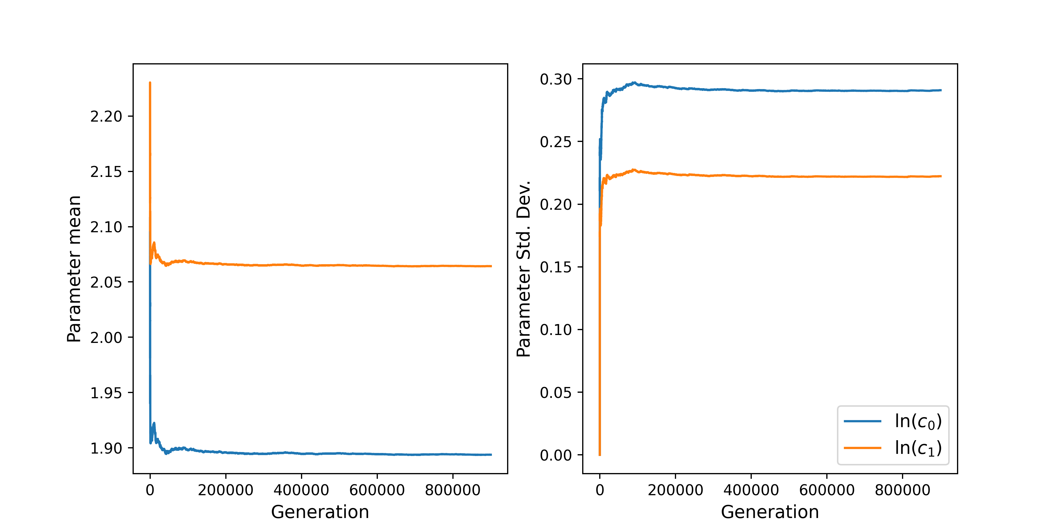
Figure 5: Parameter mean and $\sigma$ convergence with number of DE-MC generation.

3.2 Model fit and uncertainty quantification

Samples were drawn from the joint posterior distribution given in (15). For each sample, the corresponding $B/m$ and $F/m$ were calculated using the expressions in (10). The samples were then used to evaluate the model at each timestep, $t_{i}$, where the equation of motion in (6) was solved numerically to give both the position, $x$, and the velocity, $v_{x}$ ($dx/dt$). This gives a distribution for the position, $x_{i}$, and velocity, $v_{x_{i}}$, at every $t_{i}$. The mean values of $x_{i}$ and $v_{x_{i}}$ were used to produce the mean fit shown as the solid blue line in Fig. 6 with an RMSE of $0.13\text{\,}\mathrm{nm}$. In Fig. 6, the shaded regions represent the uncertainty in the positions and velocities predicted by the model, which was calculated as $\pm\,2\,\sigma$ from the distributions obtained at every $t_{i}$.

The terminal dislocation velocity $v_{t}$, was determined to be $0.15\text{\,}\mathrm{nm}\text{\,}{\mathrm{ps}}^{-1}$ from the mean fit at $t=$100\text{\,}\mathrm{ps}$$. Using $v_{t}$, the applied shear stress $\tau=$10\text{\,}\mathrm{MPa}$$, and $|\mathbf{b}|=\frac{\sqrt{2}}{2}a_{0}$, the damping coefficient, $B$, was calculated using equation (7) to be $16.8\text{\,}\mathrm{pN}\text{\,}{\mathrm{ps}}^{2}\text{\,}{\mathrm{nm}}^{-2}$. The values obtained for $v_{t}$ and $B$ compare well to those in literature [1] for the conditions used in our simulations.

Using the mean values of $c_{0}$ and $c_{1}$ obtained from the marginal parameter distributions, the corresponding values of $B/m$ and $F/m$ were calculated. These were then used with the calculated value for $B$ to calculate $m=$243.6\text{\,}\mathrm{pN}\text{\,}{\mathrm{ps}}^{2}\text{\,}{\mathrm{nm}}^{-2}$$ and $F=$2.49\text{\,}\mathrm{pN}\text{\,}{\mathrm{nm}}^{-1}$$, which corresponds to the $10\text{\,}\mathrm{MPa}$ shear stress imposed on the system. The fitted parameters and the values obtained for $v_{t}$ and corresponding $B$ recover the applied shear stress, which gives us confidence in the fitting procedure and the suitability of the model used.

It should be noted that due to the high degree of correlation between $c_{0}$ and $c_{1}$, it is not reasonable to give the uncertainty of the values for $m$, $B$ and $F$ as a simple $\pm 2\sigma$. This would lead to a significant overestimation of the uncertainty in simulation results using parameters sampled independently using those error bounds. The full uncertainty is encapsulated in the covariance matrix (15) and its effects are graphically represented in Fig. 6.

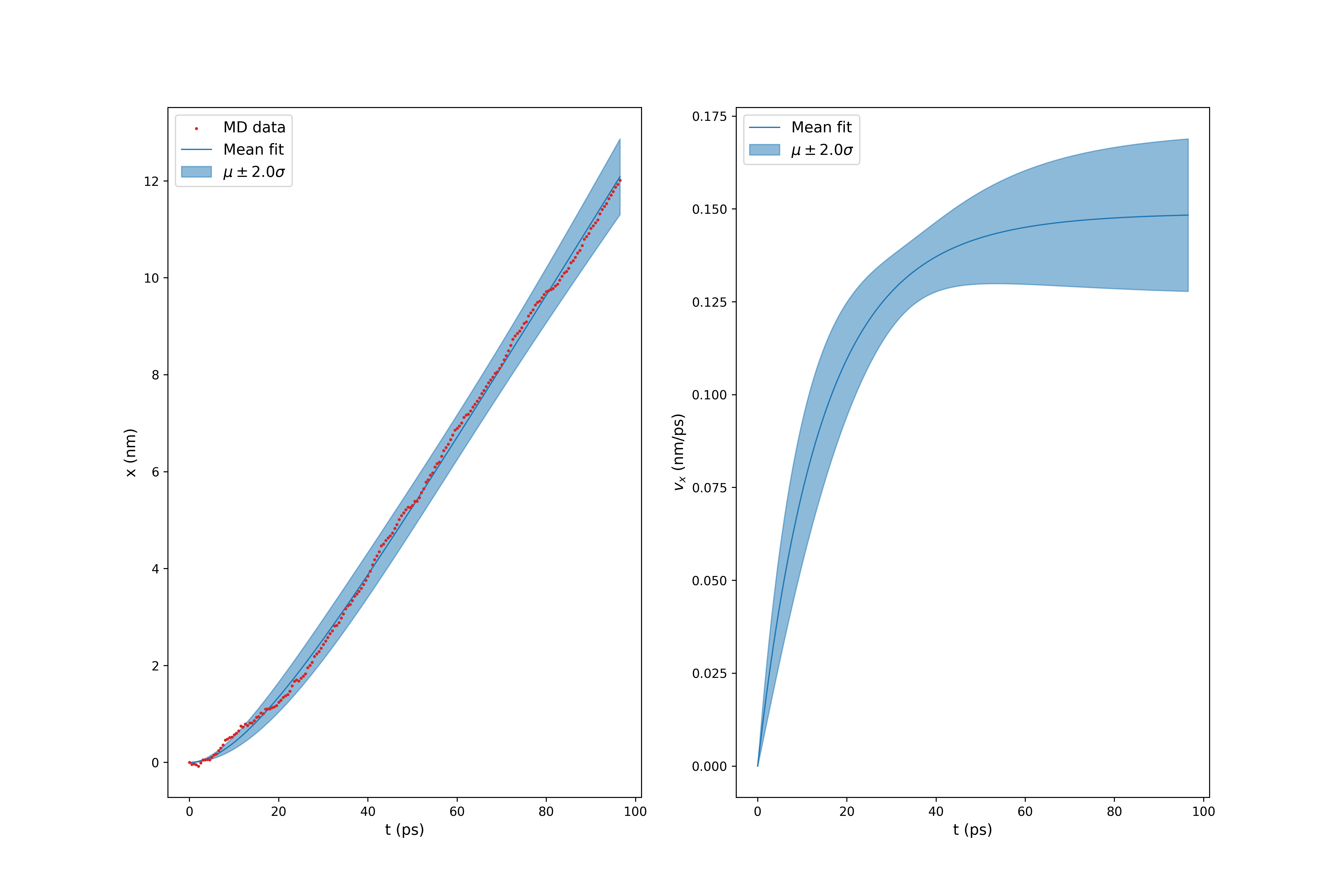
Figure 6: Model fit to the MD dislocation trajectories (position: left, velocity: right). The MD position data is shown in red. The mean fit is represented by the solid blue line, obtained by sampling the joint parameter posterior distribution. The shaded areas represent the uncertainty in the dislocation positions and velocity predicted by the model.

3.3 Current model limitations

While the method described above was able to obtain consistent values for $m$, $B$, and $F$, the approach has some limitations. In the following, we present two cases that cannot be adequately described by the simple equation of motion, but which are important for modelling material plasticity, namely the case of multiple interacting dislocations, and a dislocation interacting with an obstacle in the form of a precipitate.

3.3.1 Dislocation interactions with long-range elastic field defects

So far, we have only considered modelling the trajectory of a single dislocation in pure Ni. Dislocations are line defects with a long-range elastic field and having multiple dislocations means that their elastic fields interact. Material deformation is governed by the motion of a large number of dislocations and accordingly, realistic modelling of material deformation behaviour requires considering dislocation-dislocation interactions.

In FCC materials, $\frac{a}{2}\langle 110\rangle\{111\}$ edge dislocations are perfect dislocations, meaning they can move through the material without disrupting the lattice. In Ni-based superalloys, dislocations of this type move from the Ni solid solution matrix (modelled here as pure Ni) and can enter the $\gamma^{\prime}$ precipitates. Since $\gamma^{\prime}$ precipitates are Ni₃Al with an L1₂ structure, dislocations of this type create an anti-phase boundary (APB) when passing through them. Accordingly, $\frac{a}{2}\langle 110\rangle\{111\}$ dislocations move in pairs, where the leading dislocation creates the APB and the trailing dislocation restores the crystal structure.

In addition to dislocations travelling in pairs, another important dislocation-dislocation interaction that should be accounted for in Ni-based superalloys occurs when there are misfit dislocations forming at the interface of incoherent precipitates [12]. Due to the difference in lattice constants between the $\gamma$ ($0.352\text{\,}\mathrm{nm}$) and $\gamma^{\prime}$ ($0.357\text{\,}\mathrm{nm}$) phases [7], if the interface between these two phases is large enough, misfit dislocations form along the interface. Accordingly, dislocations from the $\gamma$ matrix encountering incoherent precipitates would also interact with these misfit dislocations.

3.3.2 Dislocation-precipitate interactions

In the pure Ni cell, the dislocation remains relatively straight throughout the simulation. However, in the presence of an obstacle, the dislocation can loop around it or it can bend if it travels through the obstacle, depending on the strengthening mechanism [13]. In Ni-based superalloys, precipitates play a major role in determining the material’s deformation behaviour by hindering dislocation motion and leading to the extraordinary strengthening effect they exhibit, especially at high temperature. In addition to the dislocation-dislocation interactions described previously, any model used to describe the deformation behaviour of Ni-based superalloys needs to also be able to capture dislocation bending due to interactions with precipitates.

4 Conclusions

In this paper, we have presented a methodology which uses DE-MC as a sampling technique to obtain the distributions of the parameters $m$, $B$, and $F$ of an equation of motion by fitting to MD dislocation trajectories. Using the methods described, we are able to obtain mean values of $B$ and $v_{t}$ that are comparable to those in literature for similar simulation conditions. Moreover, our method recovers the value of the applied shear stress that was used in the simulation. The main advantage of fitting the parameters using sampling is being able to determine the dislocation positions and velocities as a function of time while quantifying the uncertainties in the model predictions.

Based on the above, we believe that the model and fitting procedure described here work well for predicting the dislocation dynamics of straight dislocations in the absence of interactions with other dislocations and obstacles such as precipitates. We have discussed how such interactions must be described for more complex systems such as Ni-based superalloys, which is our main system of interest. This work is a first step towards building a more predictive surrogate model that is able to capture the deformation behaviour of these alloys given inputs such as precipitate size, arrangement, and morphology.

References

References

- [1] Bitzek E, Weygand D and Gumbsch P 2004 Atomistic Study of Edge Dislocations in FCC Metals: Drag and Inertial Effects IUTAM Symposium on Mesoscopic Dynamics of Fracture Process and Materials Strength Solid Mechanics and its Applications ed Kitagawa H and Shibutani Y (Dordrecht: Springer Netherlands) pp 45–57 ISBN 978-1-4020-2111-4
- [2] Bitzek E and Gumbsch P 2004 Materials Science and Engineering: A 387-389 11–15 ISSN 0921-5093 URL https://www.sciencedirect.com/science/article/pii/S0921509304004927
- [3] Bitzek E and Gumbsch P 2005 Materials Science and Engineering: A 400-401 40–44 ISSN 0921-5093 URL https://www.sciencedirect.com/science/article/pii/S0921509305002571
- [4] Cajo J F ter Braak 2006 Statistics and Computing 16 239–249 ISSN 1573-1375 URL https://doi.org/10.1007/s11222-006-8769-1
- [5] Cajo J F ter Braak and Jasper A Vrugt 2008 Statistics and Computing 18 435–446 ISSN 1573-1375 URL https://doi.org/10.1007/s11222-008-9104-9
- [6] Thompson A P, Aktulga H M, Berger R, Bolintineanu D S, Brown W M, Crozier P S, in ’t Veld P J, Kohlmeyer A, Moore S G, Nguyen T D, Shan R, Stevens M J, Tranchida J, Trott C and Plimpton S J 2022 Computer Physics Communications 271 108171 ISSN 0010-4655 URL https://www.sciencedirect.com/science/article/pii/S0010465521002836
- [7] Mishin Y 2004 Acta Materialia 52 1451–1467 ISSN 1359-6454 URL https://www.sciencedirect.com/science/article/pii/S1359645403007262
- [8] Olmsted D L, Hector L G, Curtin W A and Clifton R J 2005 Modelling and Simulation in Materials Science and Engineering 13 371 ISSN 0965-0393 URL https://dx.doi.org/10.1088/0965-0393/13/3/007
- [9] Shinoda W, Shiga M and Mikami M 2004 Physical Review B 69 134103 publisher: American Physical Society URL https://link.aps.org/doi/10.1103/PhysRevB.69.134103
- [10] Stukowski A, Bulatov V V and Arsenlis A 2012 Modelling and Simulation in Materials Science and Engineering 20 085007 ISSN 0965-0393 publisher: IOP Publishing URL https://dx.doi.org/10.1088/0965-0393/20/8/085007
- [11] Cubillos P, Harrington J, Loredo T J, Lust N B, Blecic J and Stemm M 2016 The Astronomical Journal 153 3 ISSN 1538-3881 publisher: The American Astronomical Society URL https://dx.doi.org/10.3847/1538-3881/153/1/3
- [12] Zhu T and Wang C y 2005 Physical Review B 72 014111 publisher: American Physical Society URL https://link.aps.org/doi/10.1103/PhysRevB.72.014111
- [13] Goodfellow A J 2018 Materials Science and Technology 34 1793–1808 ISSN 0267-0836 publisher: Taylor & Francis _eprint: https://doi.org/10.1080/02670836.2018.1461594 URL https://doi.org/10.1080/02670836.2018.1461594