Fitted finite element methods for singularly perturbed elliptic problems of convection-diffusion type

Abstract

Fitted finite element methods are constructed for a singularly perturbed convection-diffusion problem in two space dimensions. Exponential splines as basis functions are combined with Shishkin meshes to obtain a stable parameter-uniform numerical method. These schemes satisfy a discrete maximum principle. In the classical case, the numerical approximations converge, in $L_{\infty}$, at a rate of second order and the approximations converge at a rate of first order for all values of the singular perturbation parameter.

Keywords: Convection-diffusion, Shishkin mesh, fitted operator.

AMS subject classifications: 65N12, 65N15, 65N06.

1 Introduction

The numerical solution of singularly perturbed convection-diffusion problems of the form

$$-\varepsilon\triangle u+\vec{a}\cdot\nabla u+bu=f,\quad 0<\varepsilon\leq 1,$$

presents several computational difficulties. A key issue is to avoid spurious oscillations in the numerical approximations. These oscillations can be damped using various variants of streamline diffusion finite element methods (SDFEM) [3, 7]. However, within a finite element framework it is difficult to generate a numerical method that preserves the inverse-monotonicity of the differential operator [4] and guarantees no spurious oscillations in the numerical approximations. A significant reduction of these oscillations can be achieved by astute choices of stabilization parameters, but small oscillations can still be problematic when solving a system of nonlinear partial differential equations if one equation within the system is a singularly perturbed differential equation of convection-diffusion type. In this paper, we choose to only consider discretizations which are inverse monotone. Moreover, we are solely interested in parameter-uniform [6] numerical methods. That is, numerical methods for which an error bound on the numerical approximations $U$ of the form

$$\|u-U\|_{\infty}\leq CN^{-p},\quad p>0,$$

can be established. Here $N$ is the number of elements used in any coordinate direction, $\|\cdot\|_{\infty}$ is the pointwise $L_{\infty}$ norm and the error constant $C$ (used throughout this paper) is independent of $N$ and $\varepsilon$.

Within a finite difference (or finite volume) framework, inverse monotonicity can be retained by employing standard upwinding or variants of upwinding. However, upwinding limits the order of convergence of the numerical method to first order. For non-singularly perturbed problems with smooth solutions, second order convergence is easily achieved using central difference schemes or classical Galerkin with bilinear basis functions. For singularly perturbed problems, it is desirable that any parameter-uniform numerical method designed to be inverse-monotone would also be second order when the inverse of the singular perturbation parameter was not large compared to the dimensions of the discrete problem (i.e., if $\varepsilon^{-1}\leq CN$). In the case of singularly perturbed ordinary differential equations, fitted operator methods (which are nodally exact schemes in the case of constant coefficients) have this property at the nodes of a uniform grid. These fitted operator methods can be generated within a finite element framework by incorporating a tensor product of one dimensional exponential $L$-splines or $L^{*}$-splines into the trial or test space [20]. Hemker [10] was the first to examine these exponential basis functions. In this paper we will use these exponential splines in our choice of trial and test space.

If one employs a uniform mesh with a tensor product of one dimensional $L$-splines as basis functions in a Galerkin finite element method, then one has [19],

$$\|u-U\|_{E}\leq CN^{-1/2},$$

where $\|\cdot\|_{E}$ is the standard $\varepsilon$-weighted energy norm. For the same choice of basis functions on a uniform rectangular mesh, Dörfler [5] established error bounds in a range of $L_{p}$-norms. The numerical performance in the $L_{2}$ and $L_{\infty}$ norms, of different combinations of exponential basis functions within a Petrov-Galerkin framework (where the trial and test space are not necessarily the same), on a uniform mesh, was examined in [9]. However, as noted in [9, Remark 3.7], these schemes are not stable.

In [21], it is established that using bilinear basis functions on a Shishkin mesh [6, 15] in a Galerkin framework, yields

$$\|u-U\|_{E}\leq CN^{-1}\ln N$$

and in [23] the superclose result

$$\|u_{I}-U\|_{E}\leq C\varepsilon N^{-3/2}+C(N^{-1}\ln N)^{2}$$

is established, where $u_{I}$ is the interpolant of the continuous solution $u$ in the trial space. In [22], the same superclose bound is established for bilinear SDFEM on a Shishkin mesh. For piecewise bilinear SDFEM on a Shishkin mesh [20, pp 391], one has

$$\|u_{I}-U\|_{SD}\leq C\varepsilon N^{-3/2}+CN^{-2}(\ln N)^{2},$$

where $\|\cdot\|_{SD}$ is the steamline diffusion norm [20, pp 303]. Using an improved pointwise interpolation bounds [23] and this supercloseness result, with a finite difference argument in the corner area, one can get the following result [20, pp 400], for piecewise bilinear SDFEM on a Shishkin mesh,

$$\|u_{I}-U\|_{\infty}\leq C\varepsilon N^{-1/2}+CN^{-1}(\ln N)^{2};$$

with higher orders established within the fine mesh regions. However, none of these schemes are guaranteed to be inverse-monotone for all values of the singular perturbation parameter. In this paper, given that we design the numerical methods to be inverse-monotone, we establish estimates in the pointwise $L_{\infty}$ norm. This norm identifies all boundary and corner layer functions that can exist in the solution of singularly perturbed problems. In addition, we employ a layer adapted mesh (of Shishkin type) which means that we will achieve parameter-uniform bounds on the global pointwise error.

In this paper, we combine the benefits of a Shishkin mesh with exponential splines as basis functions. Using a Shishkin mesh with basic upwinding, yields a globally pointwise accurate numerical approximation, satisfying a parameter-uniform bound of the form [17]

$$\|u-U\|_{\infty}\leq CN^{-1}\log N.$$

The log defect in this error bound can be removed if one uses upwinding and a Bakhvalov mesh [16], instead of a Shishkin mesh. Below in the later sections, we use a tensor product of exponential basis functions on a Shishkin mesh in a finite element formulation. Within this framework, we establish the first order global $L_{\infty}$-norm error bound

$$\|u-U\|_{\infty}\leq CN^{-1}$$

and second order in the classical case of $\varepsilon=1$. Moreover, the numerical schemes satisfy a discrete maximum principle.

2 Continuous problem

Consider the singularly perturbed convection-diffusion elliptic problem

$$Lu\equiv-\varepsilon\triangle u+\vec{a}\cdot\nabla u+bu=f,\quad(x,y)\in\Omega:=(0,1)^{2};$$ (1a)

$$u=0,\quad(x,y)\in\partial\Omega;$$ (1b)

$$\vec{a}=(a_{1},a_{2}),\quad a_{1}>\alpha_{1}>0,\ a_{2}>\alpha_{2}>0;\quad b\geq 0;$$ (1c)

$$f\in C^{1,\gamma}(\overline{\Omega}),\ f(0,0)=f(1,0)=f(0,1)=f(1,1)=0.$$ (1d)

The remaining data $a_{1},a_{2},b$ are assumed to be sufficiently regular so that $u\in C^{3,\gamma}(\overline{\Omega})$ and such that only exponential boundary layers appear near the outflow edges $x=1,\ y=1$ and a simple corner layer appears in the vicinity of $(1,1)$. This corner layer is induced not by any lack of sufficient compatibility, but by the presence of the singular perturbation parameter. In this case, there is no loss in generality in dealing with homogeneous boundary data.

The solution $u$ can be decomposed [15] into the sum

$$u=v+w_{T}+w_{R}+w_{TR}.$$

Here $v$ is the regular component, $w_{R}$ is a regular boundary layer function associated with the edge $x=1$, $w_{T}$ is a regular boundary layer function associated with the edge $y=1$ and $w_{TR}$ is a corner layer function associated with the corner $(1,1)$. The decomposition into regular and layer components is defined [15, 17], so that each of the layer functions satisfy the homogeneous differential equation $Lw=0$.

By assuming the additional regularity and compatibility conditions [17]

$$a_{1},a_{2},b,,f\in C^{5,\gamma}(\overline{\Omega}),\quad\frac{\partial^{i+j}f}{\partial x^{i}\partial y^{j}}(0,0)=0,\ 0\leq i+j\leq 4$$ (1e)

on the data, one can establish the following bounds on the regular component

$$\Bigl{\|}\frac{\partial^{i+j}v}{\partial x^{i}\partial y^{j}}\Bigr{\|}_{\infty}\leq C(1+\varepsilon^{2-i-j}),\ i+j\leq 3.$$ (2)

The regular layer component $w_{R}$ is the solution of the problem

$$Lw_{R}=0,\quad(x,y)\in\Omega,$$ (3a)

$$w_{R}(1,y)=(u-v)(1,y),\quad w_{R}(0,y)=w_{L}(x,0)=0,$$ (3b)

$$w_{R}(x,1)=g(x).$$ (3c)

Using a maximum principle we can deduce that

$$|w_{R}(x,y)|\leq Ce^{-\frac{\alpha_{1}(1-x)}{\varepsilon}},\quad(x,y)\in\Omega.$$ (4a)

Using the arguments in [15, Chapter 12], coupled with the local bounds given in [12, 132–134] and the arguments in [14], one can deduce that

$$\Bigl{|}\frac{\partial^{i+j}w_{R}}{\partial x^{i}\partial y^{j}}(x,y)\Bigr{|}\leq C\varepsilon^{-i}(1+\varepsilon^{1-j})e^{-\frac{\alpha_{1}(1-x)}{\varepsilon}},\ i+j\leq 3,\ (x,y)\in\Omega.$$ (4b)

Corresponding bounds hold for $$w_{T}$$. Finally, we consider the corner layer function, which is defined as follows:

$$Lw_{TR}=0,\quad(x,y)\in\Omega,$$ (4c)

$$w_{TR}(x,0)=w_{TR}(0,y)=0,$$ (4d)

$$w_{TR}(1,y)=-w_{T}(1,y),\ w_{TR}(x,1)=-w_{R}(x,1);$$ (4e)

and we have the bounds

$$|w_{TR}(x,y)|\leq Ce^{-\frac{\alpha_{1}(1-x)}{\varepsilon}}e^{-\frac{\alpha_{2}(1-y)}{\varepsilon}},\quad(x,y)\in\Omega.$$ (4f)

Repeating the argument that led to (4b), we deduce the bounds

$$\Bigl{|}\frac{\partial^{i+j}w_{TR}}{\partial x^{i}\partial y^{j}}(x,y)\Bigr{|}\leq C\varepsilon^{-(i+j)}e^{-\frac{\alpha_{1}(1-x)}{\varepsilon}}e^{-\frac{\alpha_{2}(1-y)}{\varepsilon}},\quad i+j\leq 3,\ (x,y)\in\Omega.$$ (4g)

Remark 1.

Andreev [2] establishes this decomposition of the solution and derives bounds on the regular and layer components, while only imposing the compatibility constraints (1d), (1e) at the inflow corner $(0,0)$. No compatibility is imposed at the other three corners. However, in order to avoid dealing with the additional corner singularities at the corners $(0,1),(1,0),(1,1)$, we confine our analysis to the case where, in addition to (1e) at the inflow corner, the basic compatibility (1d) is assumed to hold at all four corners.

3 Finite element framework

A weak form of problem (1) is: find $u\in H_{0}^{1}(\Omega)$ such that

$$B(u,v)=(f,v),\ v\in H^{1}_{0}(\Omega),\qquad\hbox{where}$$ (5a)

$$B(u,v):=(\varepsilon\nabla u,\nabla v)+(\vec{a}\cdot\nabla u,v)+(bu,v);$$ (5b)

where $(u,v)$ is the standard inner product in $L^{2}$ .

The domain is discretized $\bar{\Omega}=\cup_{i,j=1}^{N}\bar{\Omega}_{i,j}$ by the rectangular elements

$$\bar{\Omega}_{i,j}:=[x_{i-1},x_{i}]\times[y_{j-1}y_{j}],1\leq i,j\leq N;$$

where the nodal points are given by the following sets

$$\bar{\omega}_{x}:=\{x_{i}|x_{i}=x_{i-1}+h_{i}\}_{i=0}^{N},\quad\bar{\omega}_{y}:=\{y_{j}|y_{j}=y_{j-1}+k_{j}\}_{j=0}^{N}.$$

We define the average mesh steps with

$$\bar{h}_{i}:=\frac{h_{i+1}+h_{i}}{2},\qquad\bar{k}_{j}:=\frac{k_{j+1}+k_{j}}{2}.$$

This mesh is a tensor product of two piecewise-uniform one dimensional Shishkin meshes [15]. The mesh $\bar{\omega}_{x}$ places $N/2$ elements into both $[0,1-\tau_{x}]$ and $[1-\tau_{x},1]$, where the transition parameters are taken to be

$$\tau_{x}=\min\{0.5,2\frac{\varepsilon}{\alpha_{1}}\ln N\}\quad\hbox{ and (analogously for $\bar{\omega}_{y}$)}\quad\tau_{y}=\min\{0.5,2\frac{\varepsilon}{\alpha_{2}}\ln N\}.$$ (6)

We denote the set of nodal points in this Shishkin mesh by

$$\Omega^{N}:=\omega_{x}\times\omega_{y}.$$

The trial and test space will be denoted by $S^{N},T^{N}\subset H_{0}^{1}(\Omega)$, respectively. The choice of trial and test functions $\{\phi_{i,j}(x,y):=\phi_{i}(x)\phi^{j}(y)\}_{i=1}^{N-1}\in S^{N},\{\psi_{i,j}(x,y):=\psi_{i}(x)\psi^{j}(y)\}_{i=1}^{N-1}\in T^{N}$ are simply a tensor product of one dimensional functions, with the following standard properties

$$0\leq\phi_{i}(x)\leq 1,\quad\phi_{i}(x_{j})=\delta_{i,j},$$

$$\hbox{supp}(\phi_{i}(x))=(x_{i-1},x_{i+1}),\quad\phi_{i}(x)+\phi_{i-1}(x)=1,\ x\in(x_{i-1},x_{i}).$$

Observe that we denote trial and test functions in the horizontal direction with subscripts and in the vertical direction with superscripts.

An approximate solution $U\in S^{N}$ to the solution of problem (5) is: find $U\in S^{N}$ such that

$$B(U,V)=(f,V),\quad\forall V\in T^{N}.$$ (7)

We denote the nodal values $U(x_{i},y_{j})$ simply by $U_{i,j}$. Hence

$$U(x,y)=\sum_{i,j=1}^{N}U_{i,j}\phi_{i}(x)\phi^{j}(y).$$

We now define $\bar{a}_{1,i}$ as piecewise constant functions, which approximate the convective coefficient $a_{1}$ by constant values on each element $\bar{\Omega}_{i,j}$. For example, one possible choice would be

$$\bar{a}_{1}(x,y)=\bar{a}_{1,i}:=\frac{a_{1}(x_{i-1},y_{j})+a_{1}(x_{i},y_{j})}{2},\ (x,y)\in(x_{i-1},x_{i}]\times(y_{j-1},y_{j}],$$

$$\bar{a}_{1}(0,y)=\bar{a}_{1}(x_{1},y),\ y\in[0,1];\quad\bar{a}_{1}(x,0)=\bar{a}_{1}(x,y_{1}),\ x\in(0,1];$$

$$\bar{a}_{2}(x,y)=\bar{a}_{2,j}:=\frac{a_{2}(x_{i},y_{j-1})+a_{2}(x_{i},y_{j})}{2},\ (x,y)\in(x_{i-1},x_{i}]\times(y_{j-1},y_{j}],$$

$$\bar{a}_{2}(0,y)=\bar{a}_{2}(x_{1},y),\ y\in(0,1];\quad\bar{a}_{2}(x,0)=\bar{a}_{2}(x,y_{1}),,\ x\in[0,1];$$

$$\bar{f}(x,y)=\bar{f}_{i,j},\quad(x,y)\in(x_{i-1},x_{i}]\times(y_{j-1},y_{j}],\ \bar{f}(x,y)=\bar{f}_{1,1},\ (x,y)\in\bar{\Omega}_{1,1}$$

$$\hbox{where}\quad\bar{f}_{i,j}:=\frac{f(x_{i-1},y_{j-1})+f(x_{i-1},y_{j})+f(x_{i},y_{j-1})+f(x_{i},y_{j})}{4};$$

$$\bar{b}(x,y)=b(x_{i},y_{j}),\ (x,y)\in(x_{i-1},x_{i}]\times(y_{j-1},y_{j}],$$

$$\bar{b}(x,y)=b(x_{1},y_{1}),\ (x,y)\in\bar{\Omega}_{1,1}.$$

Approximating the data $a_{1},a_{2},b,f$ in the weak form by the piecewise constant functions $\bar{a},\bar{b},\bar{f}$ means that all integrals (in the weak form) can be evaluated exactly.

In addition, we will lump all zero order terms, which yields increased stability and gives a simpler structure to the definition of the system matrix. That is, we introduce the additional quadrature rules

$$(a_{1}\frac{\partial\phi_{n,m}}{\partial x},\psi_{i,j}) \approx (\bar{a}_{1}\frac{\partial\phi_{n}}{\partial x}(x),\psi_{i}(x))(1,\psi^{j}(y))\delta_{m,j},$$

$$(a_{2}\frac{\partial\phi_{n,m}}{\partial y},\psi_{i,j}) \approx (\bar{a}_{2}\frac{\partial\phi^{m}}{\partial y},\psi^{j}(y))(1,\psi_{i}(x))\delta_{n,i},$$

$$(b\phi_{n,m},\psi_{i,j}) \approx b(x_{i},y_{j})(1,\psi_{i}(x))(1,\psi^{j}(y))\delta_{n,i}\delta_{m,j},$$

where $\delta_{i,j}$ is the Kronecker delta. Then we have the following quadrature rule

$$(\bar{b}U,V):=\sum_{i,j=1}^{N}b(x_{i},y_{j})U(x_{i},y_{j})V(x_{i},y_{j})(1,\psi_{i}(x))(1,\psi^{j}(y));$$

$$(\bar{a}_{1}U_{x},V):=\sum_{j=1}^{N}(\bar{a}_{1}U_{x}(x,y_{j}),V(x,y_{j}))(1,\psi^{j}(y));$$

$$(\bar{a}_{2}U_{y},V):=\sum_{i=1}^{N}(\bar{a}_{2}U_{y}(x_{i},y),V(x_{i},y))(1,\psi_{i}(x)).$$

The associated discrete weak problem is: find $U:=\sum_{i,j=1}^{N}U_{i,j}\phi_{i}(x)\phi^{j}(y)\in S^{N}$ such that

$$\bar{B}(U,\psi_{i,j})=(\bar{f},\psi_{i,j}),\quad\forall\psi_{i,j}\in T^{N};$$ (8)

$$\bar{B}(U,V):=\varepsilon(U_{x},V_{x})+\varepsilon(U_{y},V_{y})+(\bar{a}_{1}U_{x},V)+(\bar{a}_{2}U_{y},V)+(\bar{b}U,V).$$

The associated finite difference scheme to this finite element method is:

$$\sum_{n=i-1}^{i+1}\sum_{m=j-1}^{j+1}\alpha_{n,m}U_{n,m}+b(x_{i},y_{j})(1,\psi_{i,j})U_{i,j}=\sum_{n=i-1}^{i+1}\sum_{m=j-1}^{j+1}\gamma_{n,m}f(x_{n},y_{m})$$ (9a)

where the coefficients are given by:

$$\alpha_{i-1,j+1}=\alpha_{i+1,j+1}=\alpha_{i1,j-1}=\alpha_{i-1,j-1}=0$$ (9b)

$$\alpha_{i-1,j}=R^{-}_{x}(1,\psi^{j}(y))\quad\alpha_{i+1,j}=R^{+}_{x}(1,\psi^{j}(y);$$ (9c)

$$\alpha_{i,j-1}=R^{-}_{y}(1,\psi_{i}(x))\quad\alpha_{i,j+1}=R^{+}_{y}(1,\psi_{i}(x))$$ (9d)

$$\alpha_{i,i}=-(R^{-}_{x}+R_{x}^{+})(1,\psi^{j}(y))-(R^{-}_{y}+R_{x}^{y})(1,\psi_{i}(x))$$ (9e)

$$\left(\begin{array}[]{ccc}\gamma_{i-1,j+1}&\gamma_{i,j+1}&\gamma_{i+1,j+1}\\ \gamma_{i-1,j}&\gamma_{i,j}&\gamma_{i+1,j}\\ \gamma_{i-1,j-1}&\gamma_{i,j-1}&\gamma_{i+1,j-1}\end{array}\right)=\frac{1}{4}\left(\begin{array}[]{c}Q_{y}^{+}\\ Q_{y}^{C}\\ Q_{y}^{-}\end{array}\right).\left(\begin{array}[]{ccc}Q_{x}^{-}\ Q_{x}^{C}\ Q_{x}^{+}\end{array}\right).$$ (9m)

The off-diagonal matrix entries in (9b) are zero due to our use of lumping. The elements in $$R^{\pm}_{x}, Q^{\pm}_{x}$$ and are defined by

$$R_{x}^{-}:=(\phi^{\prime}_{i-1},\varepsilon\psi^{\prime}_{i}+\bar{a}_{1}\psi_{i}),\ R_{x}^{+}:=(\phi^{\prime}_{i+1},\varepsilon\psi^{\prime}_{i}+\bar{a}_{1}\psi_{i}),$$

$$R_{x}^{c}:=(\phi^{\prime}_{i},\varepsilon\psi^{\prime}_{i}+\bar{a}_{1}\psi_{i})=-R^{-}_{x}-R^{+}_{x},\quad Q_{x}^{C}:=\int_{x=x_{i-1}}^{x_{i+1}}\psi_{i}(x)\ dx,=Q_{x}^{-}+Q_{x}^{+},$$

$$Q^{-}_{x}:=\int_{x=x_{i-1}}^{x_{i}}\psi_{i}(x)\ dx,\ Q^{+}_{x}:=\int_{x=x_{i}}^{x_{i+1}}\psi_{i}(x)\ dx.$$

The elements in $$R^{\pm}_{y} Q^{\pm}_{y}$$ and are defined analogously.

We now introduce the unit $L$-spline $B(t;\rho)$ and the unit $L^{*}$-spline $B^{*}(t;\rho)$, where $\rho$ is a positive constant, as the solutions of the two point boundary value problem

$$-B_{tt}+\rho B_{t}=0,\ t\in(0,1);\quad B(0)=0,\ B(1)=1;$$

$$B^{*}_{tt}+\rho B^{*}_{t}=0,\ t\in(0,1);\quad B^{*}(0)=0,\ B^{*}(1)=1.$$

That is

$$B(t)=\frac{e^{-\rho(1-t)}-e^{-\rho}}{1-e^{-\rho}}\quad\hbox{and}\quad B^{*}(t)=\frac{1-e^{-\rho t}}{1-e^{-\rho}}.$$

Observe that the derivatives at the end-points of the interval $(0,1)$ are given by

$$B_{t}(1)=B^{*}_{t}(0)=\sigma(\rho);\ B^{*}_{t}(1)=B_{t}(0)=\sigma(-\rho);\quad\sigma(x):=\frac{x}{1-e^{-x}}.$$

Associated with these unit splines, we define the set of $\bar{L}$-spline basis functions (denoted by $B_{i,j}(x,y)$) and the the set of $\bar{L}^{*}$-spline basis functions (denoted by $B^{*}_{i,j}(x,y)$) as follows: over each computational cell $[x_{i-1},x_{i+1}]\times[y_{j-1},y_{j+1}]$

$$B_{i,j}(x,y):=\Phi_{i,j}(x)\Phi^{i,j}(y);\quad\rho_{1:i,j}:=\frac{\bar{a}_{1}(x_{i},y_{j})h_{i}}{\varepsilon};\ \rho_{2:i,j}:=\frac{\bar{a}_{2}(x_{i},y_{j})k_{j}}{\varepsilon}$$

$$\Phi_{i,j}(x):=\Bigl{\{}\begin{array}[]{ll}B(\frac{x-x_{i-1}}{h_{i}};\rho_{1:i,j}),\ x_{i-1}\leq x\leq x_{i}\\ 1-B(\frac{x-x_{i}}{h_{i+1}};\rho_{1:i+1,j}),\ x_{i}\leq x\leq x_{i+1}\end{array}$$

$$\Phi^{i,j}(x):=\Bigl{\{}\begin{array}[]{ll}B(\frac{y-y_{j-1}}{k_{j}};\rho_{2:i,j}),\ y_{j-1}\leq y\leq y_{j}\\ 1-B(\frac{y-y_{j}}{k_{j+1}};\rho_{2:i,j+1}),\ y_{j}\leq y\leq y_{j+1}\end{array}$$

The basis functions $B^{*}_{i,j}(x,y)$ are defined analogously.

If we use either $\bar{L}$-splines in the trial space and any choice of test space or $\bar{L}^{*}$-splines in the test space and any choice of trial space, then in either case we have that

$$R_{x}^{-}=-\frac{\varepsilon\sigma(\rho_{1;i,j})}{h_{i}},\ R_{x}^{+}=-\frac{\varepsilon\sigma(-\rho_{1;i+1,j})}{h_{i+1}},$$ (12a)

$$R_{y}^{-}=-\frac{\varepsilon\sigma(\rho_{2;i,j})}{k_{j}},\ R_{y}^{+}=-\frac{\varepsilon\sigma(-\rho_{2;i+1,j})}{k_{j+1}},$$ (12b)

Combined with (12), we consider the following three possible choices for the remaining terms in (9).

1. $\bar{L}^{*}$ splines in the test space and bilinear trial functions.

   $$Q^{-}_{x}=h_{i}\frac{\sigma(\rho_{1;i,j})-1}{\rho_{1;i,j}},\quad Q^{+}_{x}=h_{i+1}\frac{1-\sigma(-\rho_{1;i+1,j})}{\rho_{1;i+1,j}},$$ (13a)

2. $\bar{L}$ splines in the test space and bilinear trial functions.

   $$Q^{-}_{x}=h_{i}\frac{1-\sigma(-\rho_{1;i,j}))}{\rho_{1;i,j}},\quad Q^{+}_{x}=h_{i+1}\frac{\sigma(\rho_{1;i+1,j})-1}{\rho_{1;i+1,j}};\$$ (13b)

3. Bilinear test functions and $\bar{L}$ splines in the trial space.

   $$Q^{-}_{x}=\frac{h_{i}}{2},\ Q^{+}_{x}=\frac{h_{i+1}}{2}$$ (13c)

with analogous definitions for $Q^{+}_{y},Q^{-}_{y}$ in each case. All of these fitted schemes have an M-matrix structure and we, hence, have guaranteed stability.

Remark 2.

We can write these fitted schemes in finite difference notation as follows

$$\frac{Q^{C}_{y}}{\bar{h}_{i}\bar{k}_{j}}\bigl{(}-\varepsilon h_{i+1}D^{+}_{x}(\sigma(-\rho_{1:i,j})D^{-}_{x})+\bar{a}_{1}h_{i}D^{-}_{x}\bigr{)}U(x_{i},y_{j})$$

$$+\frac{Q^{C}_{x}}{\bar{h}_{i}\bar{k}_{j}}\bigl{(}-\varepsilon k_{j+1}D^{+}_{y}(\sigma(-\rho_{2:i,j})D^{-}_{y}+\bar{a}_{2}k_{j}D^{-}_{y}\bigr{)}U(x_{i},y_{j})$$

$$+b(x_{i},y_{j})\frac{Q^{C}_{x}Q^{C}_{y}}{\bar{h}_{i}\bar{k}_{j}}U(x_{i},y_{j})=\frac{1}{\bar{h}_{i}\bar{k}_{j}}\sum_{n=i-1}^{i+1}\sum_{m=j-1}^{j+1}\gamma_{n,m}f(x_{n},y_{m}).$$

In the case of constant coefficients $a_{1}(x,y)=\alpha_{1},a_{2}(x,y)=\alpha_{2}$ and $b(x,y)\equiv 0$, this finite difference scheme is exact for the boundary layer functions $e^{-\alpha_{1}(1-x)/\varepsilon},e^{-\alpha_{2}(1-y)/\varepsilon}$ and the corner layer function $e^{-\alpha_{1}(1-x)/\varepsilon}e^{-\alpha_{2}(1-y)/\varepsilon}$ on an arbitrary mesh.

Remark 3.

Linß  [11] examined a class of fitted finite difference operators (arising from a finite volume formulation) on a tensor product of Shishkin meshes. Using the $(L_{\infty},L_{1})$ stability argument developed by Andreev [1], Linß established that for $u\in C^{4}(\bar{\Omega})$, then

$$|(u-U)(x_{i},y_{j})|\leq CN^{-1},$$

if the fitting factor satisfies certain conditions (see [11, (3), pg. 248]). If we formally set $Q_{x}^{-}=Q_{x}^{+}=Q_{y}^{+}=Q_{y}^{+}=0,Q_{x}^{C}=\bar{h}_{i},Q_{y}^{C}=\bar{k}_{j}$ in (13), the resulting finite difference scheme scheme fits into the framework of fitted finite difference schemes analysed in Linß  [11].

Remark 4.

The above numerical schemes can also be applied to the problem

$$-\varepsilon\triangle u+a_{1}u_{x}+bu=f.$$

The solution will now have a regular layer near the outflow boundary $x=1$, two characteristic layers along the sides $y=0$ and $y=1$ and, assuming sufficient compatibility at the inflow corners, corner layers in neighbourhoods of the two outflow corners $(1,0),(1,1)$. An appropriate piecewise uniform Shishkin mesh can be constructed to capture these layers [18]. For this problem, some of the terms in the above fitted schemes simplify to

$$R^{-}_{y}=-\frac{\varepsilon}{k_{j}},R^{+}_{y}=-\frac{\varepsilon}{k_{j+1}},\quad Q^{-}_{y}=\frac{k_{j}}{2},Q^{+}_{y}=\frac{k_{j+1}}{2}.$$

4 Error analysis in $L_{\infty}$

To identify the truncation errors associated with each coordinate direction, we introduce the following notation for one dimensional differential operators

$$Lu=L_{x}u+L_{y}u+bu,$$

$$\hbox{where}\quad L_{x}u:=-\varepsilon u_{xx}+a_{1}u_{x}\quad\hbox{and}\quad L_{y}u:=-\varepsilon u_{yy}+a_{2}u_{y};$$

and their discrete counterparts

$$L^{N}U(x_{i},y_{j})=\bigl{(}\frac{Q_{y}^{C}}{\bar{k}_{j}}L^{N}_{x}+\frac{Q_{x}^{C}}{\bar{h}_{i}}L^{N}_{y}+\bar{b}_{i,j}\frac{Q^{C}_{x}Q_{y}^{C}}{\bar{h}_{i}\bar{k}_{j}}I\bigr{)}U(x_{i},y_{j});$$

$$L^{N}_{x}U(x_{i},y_{j}):=\frac{1}{\bar{h}_{i}}\bigl{(}-\varepsilon h_{i+1}D^{+}_{x}(\sigma(-\rho_{1:i,j})D^{-}_{x})+\bar{a}_{1}h_{i}D^{-}_{x}\bigr{)}U(x_{i},y_{j});$$

$$L^{N}_{y}U(x_{i},y_{j}):=\frac{1}{\bar{k}_{j}}\bigl{(}-\varepsilon k_{j+1}D^{+}_{y}(\sigma(-\rho_{2:i,j})D^{-}_{y}+\bar{a}_{2}k_{j}D^{-}_{y}\bigr{)}U(x_{i},y_{j}).$$

At each internal mesh point $(x_{i},y_{j})$, the total truncation error is

$$L^{N}(U-u)=\frac{Q^{C}_{y}}{\bar{k}_{j}}\bigl{(}L_{x}^{N}-L_{x})u+\frac{Q^{C}_{x}}{\bar{h}_{i}}\bigl{(}L_{y}^{N}-L_{y})u+(\frac{Q^{C}_{y}}{\bar{k}_{j}}-1)L_{x}u$$ (14a)

$$+(\frac{Q^{C}_{x}}{\bar{h}_{i}}-1)L_{y}u+\bar{b}(1-\frac{Q^{C}_{x}Q_{y}^{C}}{\bar{h}_{i}\bar{k}_{j}})u+\frac{1}{\bar{h}_{i}\bar{k}_{j}}(\bar{f},\psi_{i,j})-f.$$ (14b)

At each internal mesh point $(x_{i},y_{j})$, the truncation error in one coordinate direction is given by

$$(L_{x}-L_{x}^{N})u(x_{i},y_{j}) = \varepsilon\frac{(\sigma(-\rho_{1:i+1,j})-1)D_{x}^{+}u-(\sigma(-\rho_{1:i,j})-1)D_{x}^{-}u}{\bar{h}_{i}}$$ (15a)

$$+ \varepsilon(\delta_{x}^{2}u-u_{xx})+a_{1}u_{x}-\bar{a}_{1}D_{x}^{-}u-\bar{a}_{1}\frac{h_{i}-h_{i+1}}{h_{i}+h_{i+1}}D_{x}^{-}u$$

$$= a_{1}u_{x}-\bar{a}_{1}D_{x}^{-}u-\bar{a}_{1}\frac{h_{i}-h_{i+1}}{h_{i}+h_{i+1}}D_{x}^{-}u$$

$$- \varepsilon\frac{(\sigma(-\rho_{1:i,j})-\sigma(-\rho_{1:i+1,j}))}{\bar{h}_{i}}D_{x}^{-}u$$ (15b)

$$+ \varepsilon(\delta_{x}^{2}u-u_{xx})+\varepsilon(\sigma(-\rho_{1:i+1,j})-1)\delta_{x}^{2}u.$$ (15c)

Observe that

$$\varepsilon|(\sigma(-\rho_{i})-1)|\leq C\min\{h_{i},\varepsilon\};\quad|\sigma(-\rho_{i+1})-\sigma(-\rho_{i})|\leq C|\rho_{i+1}-\rho_{i})|.$$ (16)

Lemma 1.

For all three choices of test functions in (13) we have

$$\frac{1}{\bar{h}_{i}\bar{k}_{j}}|(\bar{f},\psi_{i,j})-f(x_{i},y_{j})|\leq C(h_{i}+k_{j}+\frac{h_{i}-h_{i+1}}{h_{i}+h_{i+1}}+\frac{k_{j}-k_{j+1}}{k_{j}+k_{j+1}}).$$ (17)

Proof.

For the $\bar{L}^{*}$ test functions (13a), if $p_{i}$ denotes the standard hat function then we have

$$(1,\psi_{i}-p_{i})=h_{i}\int_{s=0}^{1}\frac{1-e^{-\rho_{i}s}}{1-e^{-\rho_{i}}}-s\ ds-h_{i+1}\int_{s=0}^{1}\frac{1-e^{-\rho_{i+1}s}}{1-e^{-\rho_{i+1}}}-s\ ds$$

$$=h_{i+1}\int_{s=0}^{1}\frac{1-e^{-\rho_{i}s}}{1-e^{-\rho_{i}}}-\frac{1-e^{-\rho_{i+1}s}}{1-e^{-\rho_{i+1}}}\ ds+(h_{i}-h_{i+1})\int_{s=0}^{1}\frac{1-e^{-\rho_{i}s}}{1-e^{-\rho_{i}}}-s\ ds.$$

We bound these two terms seperately.

$$\Bigl{|}\int_{s=0}^{1}\frac{1-e^{-\rho_{i}s}}{1-e^{-\rho_{i}}}-s\ ds\Bigr{|}\leq C\min\{1,\rho_{i}\}$$ (18a)

$$\hbox{using the inequality}\quad|\frac{2(1-x-e^{-x})+x(1-e^{-x})}{2x(1-e^{-x})}|\leq C\min\{1,x\}.$$

$$\hbox{Also}\quad\Bigl{|}\int_{s=0}^{1}\frac{1-e^{-\rho_{i}s}}{1-e^{-\rho_{i}}}-\frac{1-e^{-\rho_{i+1}s}}{1-e^{-\rho_{i+1}}}\ ds\Bigr{|}\leq C\frac{|\bar{a}_{i}h_{i}-\bar{a}_{i+1}h_{i+1}|}{h_{i+1}}$$ (18b)

$$\hbox{using }\quad\bigl{|}\frac{d}{dx}\Bigl{(}\frac{1}{1-e^{-x}}-\frac{1}{x}\Bigr{)}\Bigr{|}=\bigl{|}\frac{1}{x^{2}}-\frac{e^{-x}}{(1-e^{-x})^{2}}\Bigr{|}\leq C\min\{1,\frac{1}{x}\}.$$

Hence, using $h_{i+1}\leq h_{i}$ and these two inequalities,

$$|\frac{Q^{C}_{x}}{\bar{h}_{i}}-1|=|\frac{(1,\psi_{i})}{\bar{h}_{i}}-1|\leq C(h_{i+1}+\frac{h_{i}-h_{i+1}}{h_{i}+h_{i+1}}).$$ (19a)

Likewise,

$$|\frac{Q^{C}_{y}}{\bar{k}_{j}}-1|=|\frac{(1,\psi^{j})}{\bar{k}_{j}}-1||\leq C(k_{j+1}+\frac{k_{j}-k_{j+1}}{k_{j}+k_{j+1}}).$$ (19b)

Using an analogous argument, one can see that the bounds (19a), (19b) also apply if the test functions are $L$ test functions (13b). The bounds (19a), (19b) are satisfied (trivially) if the test functions are the simple hat functions.

For any choice of the three test functions in (13)

$$(\bar{f},\psi_{i,j})-\bar{h}_{i}\bar{k}_{j}f(x_{i},y_{j}))=(\bar{f}-f(x_{i},y_{j}),\psi_{i,j})-f(x_{i},y_{j})(1,\psi_{i,j}-p_{i,j})$$

$$|(\bar{f}-f(x_{i},y_{j}),\psi_{i,j})|\leq C(h_{i}+k_{j})\bar{h}_{i}\bar{k}_{j}$$

$$(1,\psi_{i,j}-p_{i,j})=(1,\psi_{i}-p_{i})(1,\psi^{j})+(1,p_{i})(1,\psi^{j}-p^{j}))$$

$$\leq C(h_{i}+k_{j}+\frac{h_{i}-h_{i+1}}{h_{i}+h_{i+1}}+\frac{k_{j}-k_{j+1}}{k_{j}+k_{j+1}})\bar{h}_{i}\bar{k}_{j}.$$

∎

The discrete solution $U$ can be decomposed in an analogous fashion to the continuous solution. We write

$$U=V+W_{R}+W_{T}+W_{RT},\quad\hbox{where the regular component satisfies }$$

$$L^{N}V(x_{i},y_{j})=f(x_{i},y_{j}),\ (x_{i},y_{j})\in\Omega^{N},\quad V(x_{i},y_{j})=v(x_{i},y_{j})\ (x_{i},y_{j})\in\partial\Omega^{N};$$

and each of the layer functions satisfy

$$L^{N}W(x_{i},y_{j})=0,\ (x_{i},y_{j})\in\Omega^{N},\quad W(x_{i},y_{j})=w(x_{i},y_{j})\ (x_{i},y_{j})\in\partial\Omega^{N}.$$

Lemma 2.

For the regular component, the nodal error bound

$$|(V-v)(x_{i},y_{j})|\leq CN^{-1},\quad(x_{i},y_{j})\in\Omega^{N}$$

is satisfied for all three schemes in (13).

Proof.

We first bound the truncation error for the regular component and then use the discrete maximum principle and a suitable discrete barrier function to deduce the error bound.

Combining the bounds in (19a), (19b), (17) into the expression for the truncation error (14), we deduce that

$$|L^{N}(V-v)(x_{i},y_{j})|\leq C|(L_{x}^{N}-L_{x})v(x_{i},y_{j})|+C|(L_{y}^{N}-L_{y})v(x_{i},y_{j})|+$$

$$C(1+\|L_{x}v\|+\|L_{y}v\|)(h_{i}+k_{j}+\frac{h_{i}-h_{i+1}}{h_{i}+h_{i+1}}+\frac{k_{j}-k_{j+1}}{k_{j}+k_{j+1}}).$$

Using the bounds (16) in the one dimensional truncation error (15), we also have that

$$|(L_{x}-L_{x}^{N})v(x_{i},y_{j})|\leq C(1+\|v_{x}\|+\|v_{xx}\|)(h_{i}+\frac{h_{i}-h_{i+1}}{h_{i}+h_{i+1}})+Ch_{i}\varepsilon\|v_{xxx}\|.$$

Hence, using the bounds (2) on the derivatives of the regular component $v$, we have establshed the truncation error bound

$$|L^{N}(V-v)(x_{i},y_{j})|\leq C(h_{i}+k_{j}+\frac{h_{i}-h_{i+1}}{h_{i}+h_{i+1}}+\frac{k_{j}-k_{j+1}}{k_{j}+k_{j+1}}).$$

Observe that the finite difference operator $L^{N}_{x}$ can be rewritten in the form

$$L^{N}_{x}U(x_{i},y_{j})=\frac{\varepsilon}{\bar{h}_{i}}\bigl{(}\sigma(\rho_{1:i,j})D^{-}_{x}-\sigma(-\rho_{1:i+1,j})D^{+}_{x}\bigr{)}U(x_{i},y_{j}).$$

Consider the one dimensional barrier function

$$T_{x}(x_{i})=e^{-\alpha\frac{1-\sigma_{x}-x_{i}}{\varepsilon}},\ x_{i}\leq 1-\sigma_{x};\qquad T_{x}(x_{i})=1,x_{i}\geq 1-\sigma_{x}.$$

In the coarse mesh area where $x_{i}<1-\sigma_{x}$:

$$L^{N}_{x}T_{x}(x_{i})\geq\frac{\varepsilon}{H}\bigl{(}\sigma(\rho)D^{-}_{x}-\sigma(-\rho)D^{+}_{x}\bigr{)}T(x_{i})=0,\ \rho:=\frac{\alpha H}{\varepsilon};\quad\hbox{as}\quad\sigma^{\prime}(x)>0.$$

At the transition point

$$L_{x}^{N}T_{x}(1-\sigma_{x})\geq\frac{\alpha}{\bar{h}_{i}}\geq CN$$

and $L_{x}^{N}T_{x}(x_{i})=0$ in the fine mesh area where $x_{i}>1-\sigma_{x}$. We also have that, for $N$ sufficiently large,

$$L^{N}_{x}(x_{i})=\frac{\varepsilon}{\bar{h}_{i}}(\sigma_{x}(\rho_{1:i,j}))-\sigma_{x}(-\rho_{1:i+1,j}))\geq 0,\quad\forall i;$$

$$L^{N}_{x}(x_{i})=\frac{\varepsilon}{\bar{h}_{i}}(\rho_{1:i,j}+(\sigma_{x}(-\rho_{1:i,j}))-\sigma_{x}(-\rho_{1:i+1,j}))\geq\frac{a_{1}(x_{i},y_{j})}{2}\quad i\neq N/2.$$

Then, combining these two functions $x_{i},T_{x}(x_{i})$ into one barrier function, we deduce that

$$|(V-v)(x_{i},y_{j})|\leq CN^{-1}(x_{i}+T_{x}(x_{i})+y_{j}+T_{y}(y_{j}))\leq CN^{-1}.$$

∎

Consider the following fitted finite difference operator

$$L^{N}_{x,1}:=-\varepsilon\sigma(-\rho^{*}_{j})\delta_{x}^{2}+a(1,y_{j})D_{x}^{-},\quad\rho^{*}_{j}:=\frac{a(1,y_{j})h}{\varepsilon}.$$

On the fine mesh region $(1-\sigma_{x},1)\times(0,1)$

$$L^{N}_{x,1}E^{*}(x_{i},y_{j})=0,\quad\hbox{where}\quad E^{*}(x_{i},y_{j}):=e^{-\frac{a(1,y_{j})(1-x_{i})}{\varepsilon}},$$ (20)

which is a key property of the fitted operator $L^{N}_{x}$.

Lemma 3.

For the layer components, the error bounds

$$|(W_{R}-w_{R})(x_{i},y_{j})|\leq CN^{-1},\quad(x_{i},y_{j})\in\Omega^{N};$$ (21a)

$$|(W_{T}-w_{T})(x_{i},y_{j})|\leq CN^{-1},\quad(x_{i},y_{j})\in\Omega^{N};$$ (21b)

$$|(W_{TR}-w_{TR})(x_{i},y_{j})|\leq CN^{-1},\quad(x_{i},y_{j})\in\Omega^{N};$$ (21c)

are satisfied by all three schemes in (13).

Proof.

Consider the barrier function

$$B_{x}(x):=e^{-\frac{\alpha_{1}(1-x)}{2\varepsilon}},\quad\rho:=\frac{\alpha_{1}h}{\varepsilon},\ h:=\min h_{i}.$$

Then at all internal mesh points

$$L_{x}^{N}B_{x}(x_{i}) \geq \frac{\alpha_{1}}{2\bar{h}_{i}}\Bigl{(}\frac{\sigma(\rho_{i})}{\sigma(\rho/2)}-\frac{\sigma(-\rho_{i+1})}{\sigma(-\rho/2)}\Bigr{)}B_{x}(x_{i})$$

$$\geq CN(1-e^{-\rho/2})e^{-\frac{\alpha_{1}(1-x_{i})}{2\varepsilon}}>0,\quad\hbox{as}\quad\sigma^{\prime}(x)>0.$$

Hence we have the following bound on the discrete singular term $W_{R}$

$$|W_{R}(x_{i},y_{j})|\leq Ce^{-\frac{\alpha_{1}(1-x_{i})}{2\varepsilon}}.$$

Observe that in the case where the horizontal mesh is a uniform mesh (i.e., $\sigma_{x}=0.5$), then $e^{-\frac{\alpha_{1}\sigma_{x}}{2\varepsilon}}\leq N^{-1}$.

Also, by the choice of the transition parameter $\sigma_{x}$ in (6) and the pointwise bound (4a) on the layer component

$$|w_{R}(x_{i},y_{j})|\leq CN^{-2},\quad x_{i}\leq 1-\sigma_{x}.$$

Hence, for the mesh points outside the right boundary layer region,

$$|(W_{R}-w_{R})(x_{i},y_{j})|\leq CN^{-1},\quad x_{i}\leq 1-\sigma_{x}.$$

For mesh points within the side region $(1-\sigma_{x},1)\times(0,1)$, we have that the truncation error, along each level $y=y_{j}$, is

$$(L_{x}-L_{x}^{N})w_{R} = (a_{1}(x_{i},y_{j})-a_{1}(1,y_{j}))\Bigl{(}\frac{\partial w_{R}}{\partial x}-D_{x}^{-}w_{R}\Bigr{)}+(a_{1}-\bar{a}_{1})D_{x}^{-}w_{R}$$

$$- \varepsilon\frac{(\sigma(-\rho_{1:i,j})-\sigma(-\rho_{1:i+1,j}))}{h}D_{x}^{-}w_{R}+\varepsilon\bigl{(}\sigma(-\rho_{1:i+1,j})-\sigma(-\rho_{j}^{*})\bigr{)}\delta_{x}^{2}w_{R}$$

$$+ \varepsilon\bigl{(}\sigma(-\rho^{*}_{j})\delta_{x}^{2}w_{R}-\frac{\partial^{2}w_{R}}{\partial x^{2}}\bigr{)}+a_{1}(1,y_{j})\frac{\partial w_{R}}{\partial x}-a_{1}(1,y_{j}))D_{x}^{-}w_{R}.$$

We next bound some of the terms in this expression

$$\Bigl{|}(a_{1}-\bar{a}_{1})D_{x}^{-}w_{R}(x_{i},y_{j})\Bigr{|} \leq C\Bigl{|}\int_{x_{i-1}}^{x_{i}}\frac{\partial w_{R}}{\partial s}(s,y_{j})\ ds\Bigr{|}$$

$$\leq Ce^{-\frac{\alpha_{1}(1-x_{i})}{\varepsilon}}(1-e^{-\frac{\alpha_{1}h}{\varepsilon}}).$$

$$\Bigl{|}(a_{1}(x_{i},y_{j})-a_{1}(1,y_{j}))\Bigl{(}\frac{\partial w_{R}}{\partial x}-D_{x}^{-}w_{R}(x_{i},y_{j})\Bigr{)}\Bigr{|} \leq C\frac{(1-x_{i})}{\varepsilon}e^{-\frac{\alpha_{1}(1-x_{i})}{\varepsilon}}(1-e^{-\frac{\alpha_{1}h}{\varepsilon}})$$

$$\leq Ce^{-\frac{\alpha_{1}(1-x_{i})}{2\varepsilon}}(1-e^{-\frac{\alpha_{1}h}{\varepsilon}}).$$

$$\Bigl{|}\varepsilon\frac{(\sigma(-\rho_{1:i,j})-\sigma(-\rho_{1:i+1,j}))}{h}D_{x}^{-}w_{R}(x_{i},y_{j})\Bigr{|} \leq Ce^{-\frac{\alpha_{1}(1-x_{i})}{\varepsilon}}(1-e^{-\frac{\alpha_{1}h}{\varepsilon}}).$$

$$\Bigl{|}\varepsilon\bigl{(}\sigma(-\rho_{1:i+1,j})-\sigma(-\rho_{j}^{*})\bigr{)}\delta_{x}^{2}w_{R}(x_{i},y_{j})\Bigr{|} \leq C\frac{h(1-x_{i})}{\varepsilon^{2}}e^{-\frac{\alpha_{1}(1-x_{i})}{\varepsilon}}$$

$$\leq Ce^{-\frac{\alpha_{1}(1-x_{i})}{2\varepsilon}}(1-e^{-\frac{\alpha_{1}h}{\varepsilon}}).$$

The following terms remain to be bounded

$$T:=\varepsilon\sigma(-\rho^{*}_{j})\delta_{x}^{2}w_{R}-a_{1}(1,y_{j})D_{x}^{-}w_{R}+\bigl{(}-\varepsilon\frac{\partial^{2}w_{R}}{\partial x^{2}}+a_{1}(1,y_{j})\frac{\partial w_{R}}{\partial x}\bigr{)}.$$

Based on the arguments in [17, pg. 1765], we can decompose the layer component as follows

$$w_{R}(x,y)=w_{R}(1,y)e^{-\frac{a_{1}(1,y)(1-x)}{\varepsilon}}+\varepsilon z_{R}(x,y);$$

where (using the inequality $t^{n}e^{-t}\leq Ce^{-\theta t},n\geq 1,t\geq 0,0<\theta<1$ instead of using the inequality $t^{n}e^{-t}\leq Ce^{-t/2},n\geq 1,t\geq 0$ and the localized derivative bounds in [12, pp.132-134]) we can deduce that

$$\Bigl{|}\frac{\partial^{i+j}z_{R}}{\partial x^{i}\partial y^{j}}(x,y)\Bigr{|}\leq C\varepsilon^{-i}(1+\varepsilon^{-j})e^{-\frac{\alpha_{1}(1-x)}{2\varepsilon}},\ i,j\leq 3.$$ (22)

From (20), we have

$$T=\varepsilon\Bigl{(}\varepsilon\sigma(-\rho^{*}_{j})\delta_{x}^{2}z_{R}-a_{1}(1,y_{j})D_{x}^{-}z_{R}+\bigl{(}-\varepsilon\frac{\partial^{2}z_{R}}{\partial x^{2}}+a_{1}(1,y_{j})\frac{\partial z_{R}}{\partial x}\bigr{)}\Bigr{)}$$

and

$$\Bigl{|}\Bigl{(}\frac{\partial z_{R}}{\partial x}-D_{x}^{-}z_{R}\Bigr{)}\Bigr{|} \leq C\frac{1}{\varepsilon}e^{-\frac{\alpha_{1}(1-x_{i})}{2\varepsilon}}(1-e^{-\frac{\alpha_{1}h}{\varepsilon}});$$

$$\Bigl{|}\varepsilon\frac{(\sigma(-\rho_{1:i,j})-\sigma(-\rho_{1:i+1,j}))}{h}D_{x}^{-}z_{R}\Bigr{|} \leq Ce^{-\frac{\alpha_{1}(1-x_{i})}{2\varepsilon}}(1-e^{-\frac{\alpha_{1}h}{\varepsilon}});$$

$$\Bigl{|}\varepsilon\bigl{(}\sigma(-\rho_{j}^{*})-1\bigr{)}\delta_{x}^{2}z_{R}\Bigr{|} \leq C\frac{h}{\varepsilon^{2}}e^{-\frac{\alpha_{1}(1-x_{i})}{2\varepsilon}}\leq C\frac{1}{\varepsilon}e^{-\frac{\alpha_{1}(1-x_{i})}{2\varepsilon}}(1-e^{-\frac{\alpha_{1}h}{\varepsilon}});$$

$$\Bigl{|}\varepsilon\bigl{(}\frac{\partial^{2}z_{R}}{\partial x^{2}}-\delta_{x}^{2}z_{R}\bigr{)}\Bigr{|} \leq C\frac{1}{\varepsilon}e^{-\frac{\alpha_{1}(1-x_{i})}{2\varepsilon}}(1-e^{-\frac{\alpha_{1}h}{\varepsilon}}).$$

Collecting all of the bounds above, we have the following truncation error bound

$$|(L_{x}-L_{x}^{N})w_{R}(x_{i},y_{j})|\leq Ce^{-\frac{\alpha_{1}(1-x_{i})}{2\varepsilon}}(1-e^{-\frac{\alpha_{1}h}{\varepsilon}}),\quad x_{i}>1-\sigma_{x}.$$

Furthermore, using (4b), we have that

$$|(L_{y}-L_{y}^{N})w_{R}(x_{i},y_{j})|\leq C\frac{N^{-1}}{\varepsilon}e^{-\frac{\alpha_{1}(1-x_{i})}{\varepsilon}}.$$

Hence, we arrive at the truncation error bound:

$$|L^{N}(W_{R}-w_{R})(x_{i},y_{j})|\leq C\Bigl{(}\frac{N^{-1}}{\varepsilon}+(1-e^{-\frac{\alpha h}{\varepsilon}})\Bigr{)}e^{-\frac{\alpha(1-x_{i})}{2\varepsilon}},\quad x_{i}>1-\sigma_{x}.$$

In the fine mesh region where $x_{i}>1-\sigma_{x}$, we have that

$$L^{N}B_{x}(x_{i})\geq C\frac{1}{h}(1-e^{-\rho_{1}/2})e^{-\frac{\alpha_{1}(1-x_{i})}{2\varepsilon}},\qquad B_{x}(x):=e^{-\frac{\alpha_{1}(1-x)}{2\varepsilon}}.$$

Thus

$$|(W_{R}-w_{R})(x_{i},y_{j})|\leq C\Bigl{(}\frac{N^{-1}\rho}{(1-e^{-\frac{\alpha_{1}h}{\varepsilon}})}+N^{-1}\Bigr{)}B_{x}(x_{i})\leq CN^{-1}.$$

The bound on $|(W_{T}-w_{T})(x_{i},y_{j})|$ is also deduced using an analogous argument.

For the corner layer function, we can establish that

$$w_{RT}(x,y)=w_{R}(1,1)e^{-\frac{a_{1}(1,1)(1-x)}{\varepsilon}}e^{-\frac{a_{2}(1,1)(1-y)}{\varepsilon}}+\varepsilon z_{RT}(x,y);$$

where

$$\Bigl{|}\frac{\partial^{i+j}z_{RT}}{\partial x^{i}\partial y^{j}}(x,y)\Bigr{|}\leq C\varepsilon^{-(i+j)}e^{-\frac{\alpha_{1}(1-x)}{2\varepsilon}}e^{-\frac{\alpha_{2}(1-x)}{2\varepsilon}},\ i,j\leq 3.$$ (23)

Then repeating the argument from above, we deduce that

$$|(W_{RT}-w_{RT})(x_{i},y_{j})|\leq CN^{-1}.$$

∎

By combining the results from the previous two lemmas, we arrive at the nodal error bound

Theorem 1.

(Nodal convergence) If $u$ is the solution of (1), then

$$|(U-u)(x_{i},y_{j})|\leq CN^{-1},\quad(x_{i},y_{j})\in\Omega^{N};$$ (24)

where $U$ is the numerical approximation generated by any one of the three schemes in (13).

On the Shishkin mesh, this is easily extended to a global error bound using simple bilinear interpolation. If $p_{i}(x)(p^{j}(y))$ denotes the standard hat function centered at $x=x_{i}$ ($y=y_{j}$) and we denote the bilinear interpolants of the exact solution $u$ and the numerical solution $U$ by $u_{I,BL}$ and $U_{I,BL}$; then

$$u_{I,BL}(x,y):=\sum_{i,j=1}^{N}u(x_{i},y_{j})p_{i}(x)p^{j}(y),\ U_{I,BL}(x,y):=\sum_{i,j=1}^{N}U(x_{i},y_{j})p_{i}(x)p^{j}(y).$$

Note that if the trial functions are chosen as bilinear functions, then $u_{I}\equiv u_{I,BL}$ and $U\equiv U_{I,BL}$. Using the triangle inequality and the interpolation bound [21, Theorem4.2]

$$\|u-u_{I,BL}\|_{\infty}\leq C(N^{-1}\ln N)^{2}$$

on the Shishkin mesh, we easily deduce the following global error bound.

Theorem 2.

(Global convergence) If $u$ is the solution of (1), then

$$\|U-u\|_{\infty}\leq CN^{-1},$$ (25)

where $U$ is the numerical approximation generated by either the numerical method (13a) or the numerical method (13b).

For notational simplicity, we have taken the same number $N$ of elements in each coordinate direction. If one uses $N$ mesh elements in the horizontal direction and $M$ elements in the vertical direction, then one can easily establish $\|U-u\|_{\infty}\leq CN^{-1}+CM^{-1}.$

Remark 5.

The numerical method (13c) uses exponential basis functions in the trial space. Under additional regularity assumptions (assume $u\in C^{4,\gamma}(\overline{\Omega})$ and that the pointwise bounds [8, (2.8d)-(2.8f)] on the layer components $w_{R},w_{T},w_{TR}$ are valid), then one can apply the arguments in [19, Lemma 5.1] to each of the components $v,w_{R},w_{T},w_{TR}$ separately to deduce that $\|u-u_{I}\|_{\infty}\leq CN^{-1}$ for $\bar{L}$-splines on the Shishkin mesh. However, for practical reasons in our evaluation of the global accuracy of the numerical approximations, we confine our attention to bilinear interpolants in the numerical section of this paper. Note that for method (13c) the bilinear interpolant $U_{I,BL}$ will satisfy the global error bound in Theorem 2.

In the non-singularly perturbed case, we see that the schemes return to classical Galerkin with bilinear elements. Hence, we can establish the following result.

Theorem 3.

Assume that $u\in C^{4,\gamma}(\bar{\Omega})$. If $\varepsilon\geq\varepsilon_{0}>0$, where $\varepsilon_{0}$ is a fixed constant, then for all three fitted schemes in (13)

$$\|U-u\|_{\infty}\leq CN^{-2},$$ (26)

if $N$ is sufficiently large.

Proof.

When $\varepsilon\geq\varepsilon_{0}$, then

$$\Bigl{\|}\frac{\partial^{i+j}u}{\partial x^{i}\partial y^{j}}\Bigr{\|}\leq C\varepsilon_{0}^{-(i+j)}\leq C,\quad i,j\leq 4$$

and, then, $\|u-u_{I}\|_{\infty}\leq CN^{-2}.$

Let us now examine the nodal error. If $\varepsilon\geq\varepsilon_{0}>0$ and $N$ is sufficiently large, then the mesh is uniform ($h_{i}=h,\ \forall i;k_{j}=k,\ \forall j$).

We first establish the result for the scheme (13c), which simplifies

$$\bigl{(}-\varepsilon(D^{+}_{x}(\sigma(-\rho_{1:i,j})D^{-}_{x})+D^{+}_{y}(\sigma(-\rho_{2:i,j})D^{-}_{y})+\bar{a}_{1}D^{-}_{x}+\bar{a}_{2}D^{-}_{y}\bigr{)}U(x_{i},y_{j})$$

$$+b(x_{i},y_{j})U(x_{i},y_{j})=\sum_{n=i-1}^{i+1}\sum_{m=j-1}^{j+1}\gamma_{n,m}f(x_{n},y_{m});$$

$$\hbox{where}\qquad\gamma_{i-1,j-1}=\gamma_{i+1,j-1}=\gamma_{i-1,j+1}=\gamma_{i+1,j+1}=\frac{1}{16};$$

$$\gamma_{i,j-1}=\gamma_{i,j-1}=\gamma_{i-1,j}=\gamma_{i+1,j}=\frac{1}{4};\quad\gamma_{i,j}=\frac{1}{2}.$$

A standard Taylor series expansion yields

$$\bigl{|}\sum_{n=i-1}^{i+1}\sum_{m=j-1}^{j+1}\gamma_{n,m}f(x_{n},y_{m})-f(x_{i},y_{j})\bigr{|}\leq CN^{-2}.$$ (27)

Note also that, on a uniform mesh,

$$D^{-}_{x}=D_{x}^{0}-\frac{h}{2}\delta^{2}_{x};\quad\hbox{where}\quad\quad D^{0}_{x}U(x_{i},y_{j}):=\frac{U(x_{i},y_{j})-U(x_{i},y_{j})}{2h}.$$

Also

$$-\varepsilon D^{+}_{x}(\sigma(-\rho_{1:i,j})D^{-}_{x})+\bar{a}_{1:i,j}D^{-}_{x}=-\varepsilon\delta^{2}_{x}+a_{1}(x_{i},y_{j})D^{0}_{x}$$

$$+(\bar{a}_{1:i,j}-a_{1}(x_{i},y_{j}))D^{0}_{x}+\frac{\bar{a}_{1:i+1,j}-\bar{a}_{1:i,j}}{2}D^{+}_{x}+$$

$$\frac{\varepsilon}{h}\Bigl{(}(\sigma(-\rho_{1:i,j})+\frac{\rho_{1:i,j}}{2}-1)D^{-}_{x})-(\sigma(-\rho_{1:i+1,j})+\frac{\rho_{1:i+1,j}}{2}-1)D^{+}_{x})\Bigr{)};$$

and

$$(\bar{a}_{1:i,j}-a_{1}(x_{i},y_{j}))D^{0}_{x}u(x_{i},y_{j})=-\frac{h}{2}\frac{\partial a_{1}}{\partial x}(x_{i},y_{j})\frac{\partial u}{\partial x}(x_{i},y_{j})+O(h^{2});$$

$$\frac{\bar{a}_{1:i+1,j}-\bar{a}_{1:i,j}}{2}D^{+}_{x}u(x_{i},y_{j})=\frac{h}{2}\frac{\partial a_{1}}{\partial x}(x_{i},y_{j})\frac{\partial u}{\partial x}(x_{i},y_{j})+O(h^{2});$$

$$\sigma(-\rho_{1:i,j})+\frac{\rho_{1:i,j}}{2}-1=\frac{\rho_{1:i,j}}{2}\coth\Bigl{(}\frac{\rho_{1:i,j}}{2}\Bigr{)}-1=\frac{\rho^{2}_{1:i,j}}{12}+O(h^{4});$$

$$\frac{\varepsilon\rho^{2}_{1:i,j}}{h}(D^{+}_{x}-D^{-}_{x})u(x_{i},y_{j})=\varepsilon\rho^{2}_{1:i,j}\delta^{2}_{x}u(x_{i},y_{j})=O(h^{2}).$$

Collecting all these terms, we can deduce the truncation error bound

$$|L^{N}(u-U)(x_{i},y_{j})|\leq Ch^{2}+Ck^{2},$$

and the nodal error bound follows, using the discrete maximum principle. This completes the proof in the case of the scheme (13c)

In the case of the other two fitted schemes, use the inequality

$$\Bigl{|}\frac{1-e^{-sx}}{1-e^{-x}}-s\Bigr{|}\leq Cx^{2},\quad 0\leq s\leq 1,\ x>0$$

to establish that, when $\varepsilon\geq\varepsilon_{0}$, that

$$|\frac{Q^{C}_{x}}{h}-1|\leq Ch^{2}\quad\hbox{and}\quad|\frac{Q^{C}_{y}}{k}-1|\leq Ck^{2}.$$

Complete the proof as above.

∎

5 Numerical examples

In this final section, we will estimate the global (as opposed to the nodal) accuracy of our numerical methods.

Example 1 Consider the following constant coefficient test problem:

$$-\varepsilon\triangle u+2u_{x}+3u_{y}=f,(x,y)\in\Omega;\ u=0,\ (x,y)\in\partial\Omega,$$ (28)

where $f$ is such that the exact solution is

$$u(x,y)=\Bigl{(}x-\frac{e^{2x/\varepsilon}-1}{e^{2/\varepsilon}-1}\bigr{)}\bigl{(}y-\frac{e^{3y/\varepsilon}-1}{e^{3/\varepsilon}-1}\bigr{)}+\sin(\pi x)\sin(\pi y).$$

A sample plot of the computed solution using the numerical scheme (13a) is displayed in Figure 1 and the corresponding global error is displayed in Figure 2.

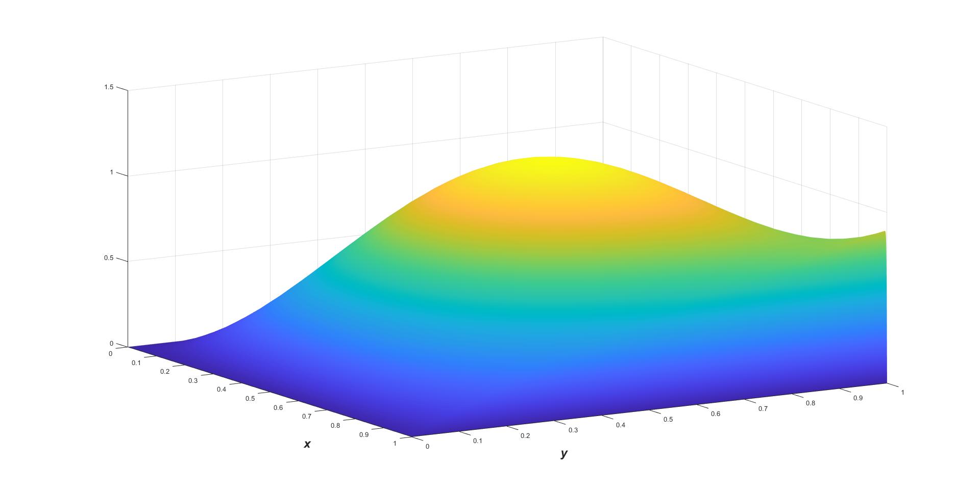
Figure 1: Computed solution with the numerical scheme (13a) applied to problem (28) for $\varepsilon=2^{-10}$ and $N=M=64$

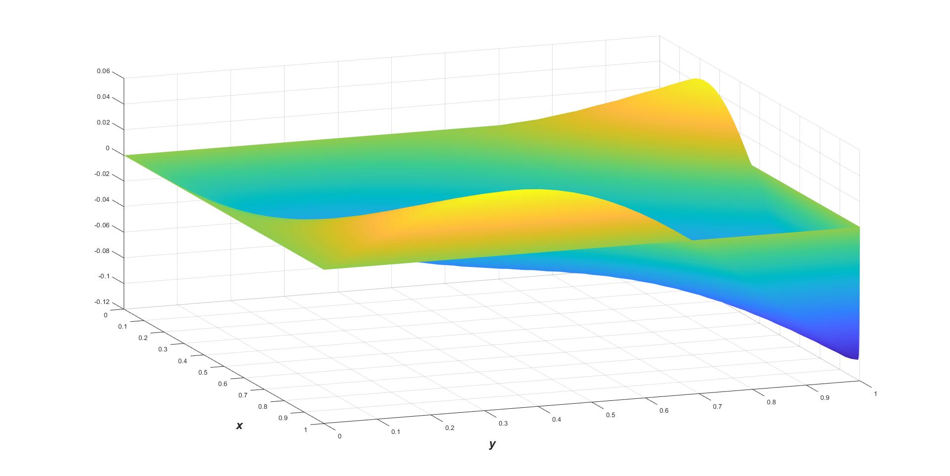
Figure 2: Global error with the numerical scheme (13a) applied to problem (28) for $\varepsilon=2^{-10}$ and $N=M=64$

In the case of the three fitted schemes and simple upwinding on the Shishkin mesh, the global errors are estimated by calculating the maximum error over a fine Shishkin mesh. That is,

$$\|U-u\|\approx E^{N}_{\varepsilon}:=\max_{(x_{i},y_{j})\in\Omega^{2048}_{S}}|(U_{I,BL}-u)(x_{i},y_{j})|$$

The global errors in Tables 1,2,3 for the fitted schemes (13a), (13b) and (13c) indicate first order convergence for this constant coefficient problem and second order convergence for $\varepsilon$ of order one. These errors can be compared to the global errors in Table 4 for simple upwinding on the same Shishkin mesh. For large values of $\varepsilon$, the fitted schemes are a significant improvement on basic upwinding. Overall, the fitted scheme (13a) performs best for this test problem. These numerical results are in agreement with the theoretical error bounds established in Theorem 3. We estimate the global orders of local convergence using the double-mesh principle [6, §8.6]. The orders of global convergence for (13a) in Table 5 can be compared to the global orders of convergence of simple upwinding in Table 6.

Example 2 Consider the variable coefficient problem

$$-\varepsilon\triangle u+(2+x+x^{2}+3xy)u_{x}+(3+y+y^{2}+2xy)u_{y}=16x(1-x)y(1-y))$$ (29)

with $u=0$ on the boundary. The orders of global convergence in Table 7 for the fitted scheme (13a) indicate first order convergence. These orders should be compared to the orders for standard upwinding in Table 8 on the same Shishkin mesh, where the $\log$ defect in the orders is evident.

Table 1: Global errors $E^{N}_{\varepsilon}$ for the scheme (13a) applied to problem (28)

$\varepsilon|N$	$N=8$	16	32	64	128	256	512	1024
$2^{0}$	0.0666	0.0170	0.0043	0.0011	0.0003	0.0001	0.0000	0.0000
$2^{-4}$	0.3201	0.1305	0.0408	0.0098	0.0022	0.0005	0.0001	0.0000
$2^{-8}$	0.4463	0.3148	0.1831	0.0957	0.0444	0.0171	0.0052	0.0014
$2^{-12}$	0.4601	0.3296	0.1982	0.1103	0.0581	0.0295	0.0145	0.0069
$2^{-16}$	0.4610	0.3305	0.1992	0.1112	0.0590	0.0303	0.0153	0.0077
$2^{-20}$	0.4610	0.3306	0.1993	0.1113	0.0591	0.0304	0.0154	0.0077

Table 2: Global errors $E^{N}_{\varepsilon}$ for the scheme (13b) applied to problem (28)

$\varepsilon|N$	$N=8$	16	32	64	128	256	512	1024
$2^{0}$	0.0754	0.0196	0.0049	0.0012	0.0003	0.0001	0.0000	0.0000
$2^{-4}$	0.9269	0.3724	0.1075	0.0260	0.0059	0.0013	0.0003	0.0001
$2^{-8}$	1.1373	0.7007	0.3563	0.1703	0.0771	0.0303	0.0096	0.0026
$2^{-12}$	1.1545	0.7246	0.3769	0.1911	0.0980	0.0493	0.0243	0.0116
$2^{-16}$	1.1556	0.7261	0.3782	0.1926	0.0993	0.0506	0.0255	0.0128
$2^{-20}$	1.1557	0.7262	0.3783	0.1927	0.0994	0.0506	0.0256	0.0128

Table 3: Global errors $E^{N}_{\varepsilon}$ for the scheme (13c) applied to problem (28)

$\varepsilon|N$	$N=8$	16	32	64	128	256	512	1024
$2^{0}$	0.0710	0.0181	0.0046	0.0011	0.0003	0.0001	0.0000	0.0000
$2^{-4}$	0.5840	0.2380	0.0703	0.0173	0.0039	0.0009	0.0002	0.0000
$2^{-8}$	0.7150	0.4598	0.2575	0.1302	0.0595	0.0231	0.0072	0.0019
$2^{-12}$	0.7200	0.4798	0.2768	0.1479	0.0759	0.0381	0.0187	0.0089
$2^{-16}$	0.7202	0.4811	0.2781	0.1490	0.0770	0.0391	0.0196	0.0098
$2^{-20}$	0.7203	0.4812	0.2781	0.1491	0.0770	0.0391	0.0197	0.0099

Table 4: Global errors $E^{N}_{\varepsilon}$ for simple upwinding applied to problem (28)

$\varepsilon|N$	$N=8$	16	32	64	128	256	512	1024
$2^{0}$	0.1245	0.0703	0.0372	0.0191	0.0097	0.0049	0.0024	0.0012
$2^{-4}$	0.6516	0.3804	0.2069	0.1116	0.0598	0.0319	0.0170	0.0090
$2^{-8}$	0.7913	0.4592	0.2569	0.1417	0.0780	0.0422	0.0226	0.0120
$2^{-12}$	0.7994	0.4653	0.2602	0.1434	0.0790	0.0428	0.0229	0.0122
$2^{-16}$	0.7999	0.4656	0.2604	0.1436	0.0790	0.0428	0.0229	0.0122
$2^{-20}$	0.7999	0.4657	0.2604	0.1436	0.0790	0.0428	0.0229	0.0122

Table 5: Orders of global convergence for the scheme (13a) applied to problem (28)

$\varepsilon|N$	$N=8$	16	32	64	128	256	512
$2^{0}$	1.9025	1.9762	1.9943	1.9987	1.9997	2.0000	2.0000
$2^{-4}$	1.2654	1.6719	1.9879	1.7876	1.6014	1.6438	1.6834
$2^{-8}$	0.8021	0.5796	0.8045	0.9202	1.2133	1.6216	1.8799
$2^{-12}$	0.7724	0.5813	0.7981	0.8801	0.9403	0.9742	0.9906
$2^{-16}$	0.7704	0.5813	0.7975	0.8797	0.9398	0.9740	0.9899
$2^{-20}$	0.7703	0.5813	0.7975	0.8797	0.9398	0.9740	0.9898
Uniform	0.9004	0.5813	0.7975	0.8797	0.9398	0.9740	0.9898

Table 6: Orders of global convergence for upwinding applied to problem (28)

$\varepsilon|N$	$N=8$	16	32	64	128	256	512
$2^{0}$	1.1033	1.0507	1.0286	1.0148	1.0075	1.0037	1.0019
$2^{-4}$	0.7810	0.9087	0.9019	0.9085	0.9134	0.9193	0.9189
$2^{-8}$	0.8370	0.8311	0.8458	0.8674	0.8775	0.8956	0.9074
$2^{-12}$	0.8355	0.8268	0.8418	0.8713	0.8752	0.8946	0.9064
$2^{-16}$	0.8354	0.8263	0.8419	0.8715	0.8751	0.8945	0.9063
$2^{-20}$	0.8354	0.8262	0.8419	0.8715	0.8751	0.8945	0.9063
Uniform	0.8354	0.8262	0.8419	0.8715	0.8751	0.8945	0.9063

Table 7: Orders of global convergence for the scheme (13a) applied to problem (29)

$\varepsilon|N$	$N=8$	16	32	64	128	256	512
$2^{0}$	1.9297	1.9604	1.9844	1.9930	1.9967	1.9984	1.9992
$2^{-4}$	0.5233	0.8485	1.1258	1.3165	1.4590	1.5645	1.6393
$2^{-8}$	0.3879	0.6967	1.0264	1.2831	1.4689	1.3243	1.6966
$2^{-12}$	0.3807	0.6921	1.0227	1.2796	1.3505	0.9298	0.9505
$2^{-16}$	0.3802	0.6917	1.0224	1.2794	1.3496	0.9295	0.9502
$2^{-20}$	0.3801	0.6917	1.0224	1.2794	1.3496	0.9295	0.9501
Uniform	0.4410	0.6917	1.0224	1.2794	1.3496	0.9295	0.9501

Table 8: Orders of global convergence for standard upwinding applied to the test problem (29)

$\varepsilon|N$	$N=8$	16	32	64	128	256	512
$2^{0}$	0.8903	0.9471	0.9710	0.9847	0.9919	0.9959	0.9979
$2^{-4}$	0.3737	0.5625	0.6500	0.6954	0.7152	0.8034	0.8202
$2^{-8}$	0.3337	0.5258	0.5879	0.6735	0.7304	0.8087	0.8301
$2^{-12}$	0.3299	0.5229	0.5821	0.6726	0.7317	0.8097	0.8303
$2^{-16}$	0.3298	0.5227	0.5817	0.6726	0.7318	0.8098	0.8303
$2^{-20}$	0.3298	0.5227	0.5817	0.6726	0.7318	0.8098	0.8303
Uniform	0.3298	0.5227	0.5817	0.6726	0.7318	0.8098	0.8303

References

• [1] V. B. Andreev, Anisotropic estimates for the Green function of a singularly perturbed two-dimensional monotone difference convection-diffusion operator and their applications, Zh. Vychisl. Mat. Mat. Fiz., 43 (4), (2003), 546–553.
• [2] V. B. Andreev, Uniform grid approximation of nonsmooth solutions of a singularly perturbed convection-diffusion equation in a rectangle, Differ. Uravn., 45 (7), (2009), 954–964.
• [3] M. Augustin, A. Caiazzo, A. Fiebach, J. Fuhrmann, V. John, A. Linke and R. Umla, An assessment of discretizations for convection-dominated convection-diffusion equation, Comput. Methods Appl. Mech. Engrg., 200 (47-48), (2011), 3395–3409.
• [4] G. Barrenechea, V. John, P. Knobloch and R. Rankin, A unified analysis of algebraic flux correction schemes for convection-diffusion equations, SeMA Journal. Boletin de la Sociedad Espanñola de Matemática Aplicada, 75 (4), (2018), 655–685.
• [5] W. Dörfler, Uniform error estimates for an exponentially fitted finite element method for singularly perturbed elliptic equations, SIAM J. Numer. Anal., 36 (6), (1999), 1709–1738,
• [6] P.A. Farrell, A.F. Hegarty, J.J.H. Miller, E. O’Riordan and G.I. Shishkin, Robust computational techniques for boundary layers, CRC Press, 2000.
• [7] D. Frerichs and V. John, On reducing spurious oscillations in discontinuous Galerkin (DG) methods for steady-state convection-diffusion equations, J. Comput. Appl. Math., 2021, 113487.
• [8] J.L. Gracia and E. O’ Riordan, Scaled discrete derivatives of singularly perturbed elliptic problems, Numer. Meth. Part. Diff. Eq., 31 (1), (2015), 225–252.
• [9] A. F. Hegarty, E. O’Riordan and M. Stynes A comparison of uniformly convergent difference schemes for two-dimensional convection-diffusion problems. J. Comput. Phys., 105, (1993), 24–32.
• [10] P. W. Hemker, A numerical study of stiff two-point boundary problems, Mathematical Centre Tracts, No. 80, Amsterdam, 1977.
• [11] T. Linß, Uniform pointwise convergence of an upwind finite volume method on layer-adapted meshes, ZAMM Z. Angew. Math. Mech., 82 (4), (2002), 247–254.
• [12] O.A. Ladyzhenskaya and N.N. Ural’tseva, Linear and Quasilinear Elliptic Equations, Academic Press, New York and London, 1968.
• [13] T. Linß and M. Stynes, Asymptotic analysis and Shishkin-type decomposition for an elliptic convection-diffusion problem, J. Math. Anal. and Applications, 261, (2001), 604–632.
• [14] J.J.H. Millerr, E. O’Riordan and G. I. Shishkin and L. P. Shishkina, Fitted mesh methods for problems with parabolic boundary layers, Mathematical Proceedings of Royal Irish Academy, 98A, (2), (1998), 173-190.
• [15] J.J.H. Miller, E. O’Riordan and G.I. Shishkin, Fitted Numerical Methods for Singular Perturbation Problems, World-Scientific, Singapore (Revised edition), 2012.
• [16] T. A. Nhan and R. Vulanović, The Bakhvalov mesh: a complete finite-difference analysis of two-dimensional singularly perturbed convection-diffusion problems, Numer. Algorithms, 87(1), (2021), 203–221.
• [17] E. O’Riordan and G. I. Shishkin, A technique to prove parameter–uniform convergence for a singularly perturbed convection–diffusion equation, J. Comput. Appl. Math., 206, (2007), 136–145.
• [18] E. O’Riordan and G. I. Shishkin, Parameter uniform numerical methods for singularly perturbed elliptic problems with parabolic boundary layers, Appl. Num. Math., 58, (2008), 1761-1772.
• [19] E. O’Riordan and M. Stynes, A globally uniformly convergent finite element method for a singularly perturbed elliptic problem in two dimensions, Math. Comp., 57 (195), (1991), 47-62.
• [20] H. G. Roos, M. Stynes and L. Tobiska, Robust numerical methods for singularly perturbed differential equations, Springer Series in Computational Mathematics, 24, Second edition, 2008.
• [21] M. Stynes and E. O’Riordan, A uniformly convergent Galerkin method on a Shishkin mesh for a convection-diffusion problem, J. Math. Anal. Appl., 214, (1997), 36-54.
• [22] M. Stynes and L. Tobiska, The SDFEM for a convection-diffusion problem with a boundary layer: optimal error analysis and enhancement of accuracy, SIAM J. Numer. Anal., 41 5, (2003), 1620–1642.
• [23] Z. Zhang, Finite element superconvergence on Shishkin mesh for 2-D convection-diffusion problems, Math. Comp., 72 (243), (2003), 1147–1177.