COIN-LIO: Complementary Intensity-Augmented LiDAR Inertial Odometry

Abstract

We present COIN-LIO, a LiDAR Inertial Odometry pipeline that tightly couples information from LiDAR intensity with geometry-based point cloud registration. The focus of our work is to improve the robustness of LiDAR-inertial odometry in geometrically degenerate scenarios, like tunnels or flat fields. We project LiDAR intensity returns into an intensity image, and propose an image processing pipeline that produces filtered images with improved brightness consistency within the image as well as across different scenes. To effectively leverage intensity as an additional modality, we present a novel feature selection scheme that detects uninformative directions in the point cloud registration and explicitly selects patches with complementary image information. Photometric error minimization in the image patches is then fused with inertial measurements and point-to-plane registration in an iterated Extended Kalman Filter. The proposed approach improves accuracy and robustness on a public dataset. We additionally publish a new dataset, that captures five real-world environments in challenging, geometrically degenerate scenes. By using the additional photometric information, our approach shows drastically improved robustness against geometric degeneracy in environments where all compared baseline approaches fail.

I INTRODUCTION

Recent advances in 3D LiDAR have decreased both the size and price of these sensors, enabling them to be used by a wider range of robots. At the same time, new LiDAR-based state estimation approaches such as FAST-LIO2 [1] have increased the accuracy and robustness while decreasing the computational cost, making 3D LiDAR one of the most popular choices for mobile robot sensors, especially in GNSS-denied environments. However, even these LIO approaches struggle in geometrically degenerate environments, such as tunnels, flat fields, and planar environments.

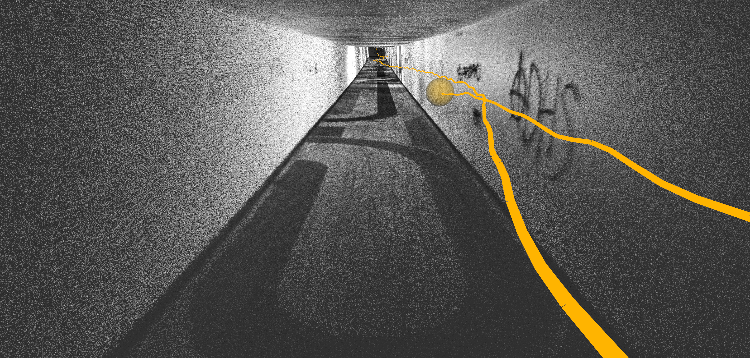
trim=0 .50pt 0 0,clip

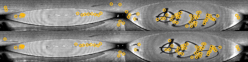
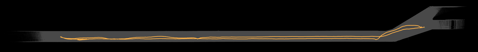
Figure 1: Top: Accumulated point cloud colorized by intensity and trajectory (orange) resulting from COIN-LIO. Our approach achieves accurate odometry despite geometric degeneracy along the tunnel, resulting in clearly visible correct ground and wall markings. Mid: Filtered intensity with tracked features (orange). Bottom: Top view of the resulting point cloud (gray) and trajectory (orange) from the tunnel.

In most geometrically uninformative scenes in the real world, the texture of the environment still offers some visual information. While other work [2, 3, 4, 5] has focused on fusing camera information with LiDAR to take advantage of this complementary data , this requires additional sensors, accurate extrinsic calibration, and time synchronization. Cameras are also passive sensors that will not work in the absence of ambient light, which limits their applicability. However, in addition to range measurements, modern 3D LiDARs also provide the measured return strength of each reflected point (intensity). For rotating multi-layer LiDARs, this signal can be projected into a dense image, which allows the LiDAR to operate as an active camera without external illumination. Images and point clouds are time-synchronized and the extrinsics are known, which further simplifies their use.

These intensity images contain texture information about the environment, which can be used to inform pose estimation in geometrically degenerate environments. Compared to camera images, LiDAR intensity images suffer from poor Signal-to-Noise Ratio, lower resolution, strong rolling shutter effects (as a rotating LiDAR spins much slower than a camera sensor exposes), and a different projection model from traditional pinhole cameras, making it difficult to directly apply visual odometry methods.

We present COIN-LIO, a robust, real-time intensity-augmented LIO framework, that couples geometric registration with photometric error minimization for improved robustness. We improve upon related work by introducing a filtering method to improve brightness consistency in the intensity image and an intensity feature selection scheme that complements geometrically degenerate directions. This feature selection is important as geometrically-degenerate parts of the scene (like tunnel edges) are often also visually degenerate. This allows us to vastly increase robustness of the combined method in geometrically degenerate scenarios, while keeping or improving performance in easier cases.

We found a lack of 3D LiDAR datasets focusing on scenarios with degenerate geometry. To this end, we created the ENWIDE dataset, that captures five real-world ENvironments WIth large sections of DEgenerate geometry and recorded ground truth positions from a high accuracy laser scanner. We hope that by providing this data to the community along with our open-sourced code implementation, we can fuel further advances in robust LiDAR-inertial odometry.

The main contributions of our work are: (1) we show that our approach that effectively leverages LiDAR intensity improves robustness and performance of LIO in geometrically degenerate scenes, (2) we propose a LiDAR-intensity image processing pipeline as well as a geometrically complementary feature selection scheme that allows us to detect and track salient features with complementary information to the geometry-based measurements, (3) we provide a real-world dataset, ENWIDE, that contains ten sequences in five scenes of diverse geometrically degenerate environments, with accurate position ground truth.

We present our contributions in a combined system with geometry-based LIO, based on FAST-LIO2 [1], and show superior performance on a standard dataset and ENWIDE, over geometry-only and geometry-and-intensity-based methods.

II Related Work

II-A LiDAR (Intertial) Odometry

Common LiDAR-based odometry approaches are based on registration of a measured point cloud against a (sub)map that is built during operation. It is computationally not feasible to register and map all points that modern 3D LiDARs produce online. For many years, the standard approach for LO was LOAM [6] which extracts points on edges and planes for registration. This works well in structure-rich environments, but such edge and plane points are often not expressive enough to perform robustly in geometrically challenging scenarios. KISS-ICP [7] avoids feature selection and directly registers a voxel-downsampled point cloud with point-to-point ICP which showed improved performance in unstructured environments. X-ICP [8] explicitly detects degenerate directions in the registration, but relies on an auxiliary state estimate. The additional use of inertial measurements in LIO approaches has shown a large increase in robustness, as it allows accurately undistorting the point cloud from ego-motion and provides an initial guess for the registration. LIO-SAM [9] fuses IMU measurements in a factor-graph [10, 11] with edge and plane feature matching against submaps. FAST-LIO [12] presents an efficient formulation of the Kalman Filter update that allows for alignment of every scan against the continuously built map in real-time. The authors switch from feature matching to raw points with point-to-plane ICP in its successor [1] that achieves state-of-the-art performance, which we base our approach on.

II-B Intensity Assisted Odometry

Several approaches use intensity as a similarity metric and integrate it into a weighted ICP [13, 14] or use high-intensity points as an additional feature class [15, 16, 17]. These approaches cannot capture fine-grained details due to their lower map resolution. The approaches presented in [18, 19] detect and match image features in the intensity image and only use the corresponding points for registration. However, in geometrically degenerate cases such features are often sparse and therefore most of the geometric information is neglected which can result in inferior performance. In the approaches above, the intensity only influences the point correspondences, but does not directly provide a gradient in the optimization. Differently, in MD-SLAM [20], the photometric error of the intensity image is optimized together with a range and normal image; however they do not use the IMU or perform motion undistortion and evalute the entire dense image instead of sparse informative patches as in our work. The approach closest to our work is RI-LIO [21]. Similar to us, they integrate photometric error minimization into the iEKF [22] of [1], but use reflectivity instead of intensity. They randomly downsample the point cloud and project single points stored in a downsampled map into the reflectivity image for the photometric components. However, relevant information is typically not distributed homogeneously in images but concentrated in specific salient regions. Instead of single random pixels at a low resolution, we specifically select geometrically complementary, salient high-resolution patches from a filtered image and continuously asses feature validity. This leads to superior performance in difficult geometrically-deficient scenarios compared to existing approaches.

III Method

Figure 2: Projection model. The offset between LiDAR origin and laser emitter is denoted as $r$. A measured point is depicted on the top right ($p$).

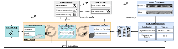
Figure 3: System Overview: The input point cloud is used geometrically (green) for map registration and as a projected image (blue) for photometric error minimization. Both residuals are combined in an iterated update (orange). We use the registration Jacobian to find uninformative directions in the geometry and select features with complementary image information (right bottom). Lines indicate information flow before (- - -) and after (—) the update step.

COIN-LIO adopts the tightly-coupled iterated Extended Kalman Filter presented in FAST-LIO2 for the point-to-plane registration and extends it using photometric error minimization. However, our approach could be applied to other LIO frameworks as well. Due to space limitations we do not review FAST-LIO2, but refer the reader to their works [12, 1] and focus on the photometric component instead. We process intensity images from point clouds using a novel filter that improves brightness consistency and reduced sensor artifacts. We specifically select image features that provide information in uninformative directions of the point cloud geometry. The feature management module examines the validity of tracked features and detects occlusions. Finally, we integrate the photometric residual into the Kalman Filter.

III-A Definitions

We define a fixed global frame ($\mathit{G}$) at the initial pose of the IMU ($\mathit{I}$). The transformation from LiDAR frame ($\mathit{L}$) to IMU frame is assumed to be known as $\mathbf{T}_{IL}=(\mathbf{R}_{IL},{}_{I}\mathbf{p}_{IL})\in\mathit{SE}(3)$. We define the robot’s state as $\mathbf{x}=[\mathbf{R}_{GI},{}_{G}\mathbf{p}_{GI},{}_{G}\mathbf{v}_{I},\mathbf{b}^{a},\mathbf{b}^{g},{}_{G}\mathbf{g}],$ where $\mathbf{R}\in\mathit{SO}(3)$ denotes orientation, $\mathbf{p}\in\mathbb{R}^{3}$ is the position, $\mathbf{v}\in\mathbb{R}^{3}$ describes linear velocity, and $\mathbf{b}^{a},\mathbf{b}^{g}\in\mathbb{R}^{3}$ indicate accelerometer and gyro biases. Each LiDAR scan consists of points recorded during one full revolution $\mathcal{P}=\{{}_{L_{j}}\mathbf{p}_{j},j=1,...,k\}$, with $t_{j}\leq t_{k}$.

III-B IMU Prediction and point cloud undistortion

We adopt the Kalman Filter prediction step according to FAST-LIO2 [1] by propagating the state using IMU measurement integration from $t_{j}$ to $t_{k}$. Similarly, we calculate the ego-motion compensated, undistorted points at the latest timestamp $t_{k}$ as: ${}_{L_{k}}\mathbf{p}_{j}=\mathbf{T}_{L_{k}I_{k}}\mathbf{T}_{I_{k}I_{j}}\mathbf{T}_{I_{j}L_{j}}{}_{L_{j}}\mathbf{p}_{j}$.

III-C Image Projection Model

We project ${}_{L_{j}}\mathbf{p}_{j}=[x_{j},y_{j},z_{j}]$ to image coordinates using:

where $L_{j}=\sqrt{x_{j}^{2}+y_{j}^{2}}-r$, $R_{j}=\sqrt{L_{j}^{2}+z_{j}^{2}}$, $\mathit{f}_{x}=\frac{-w}{2\pi}$, $\mathit{f}_{y}=\frac{-h}{\Theta_{fov}}$ as illustrated in Figure 2, and $w$ and $h$ denote horizontal and vertical resolution of the LiDAR. Due to irregular vertical beam spacing in the LiDAR, this results in empty pixels as outlined in [21]. Thus, we directly create the image from laser beam and encoder value and compensate the horizontal offset similar to [21], but use a constant value for all beams. We keep a list of all beam-elevation angles $\Theta_{L}=\{\theta_{1},...,\theta_{h}\}$ from the calibration of the LiDAR. When we project a feature point into the image, we calculate $\theta_{f}$ and find the beams above and below in $\Theta_{L}$ to interpolate the subpixel coordinate.

III-D Image Processing

The irregular vertical beam spacing causes horizontal line artifacts in the intensity image. They are less apparent in structure-rich scenes, but dominate the image in environments with little structure. As they occur at a regular row-frequency we design a finite impulse response filter to remove them. First, we use a highpass filter vertically with cutoff just below the line frequency. Apart from the lines, the output also contains relevant image content at this frequency. We therefore apply a lowpass filter horizontally, which isolates the lines as relevant image signals appear at a higher horizontal frequency. Finally, we subtract the isolated signal from the intensity image. Intensity values depend on the reflectivity of the surface as well as the distance and incidence angle. The intensity is thus lower in areas that are farther away from the sensor. LiDARs such as the Ouster also report compensated reflectivity signals, which is used in [21], but the influence of the incidence angle remains. We therefore propose a different approach to achieve consistent brightness throughout the image.

The brightness level varies smoothly throughout the image, as average distance and incidence angle are typically driven by the global structure of the scene instead of small geometric details. We thus build a brightness map $\mathit{I}_{b}(u,v)$ by averaging the intensity values in a large window. To achieve consistent exposure throughout the image, we calculate the filtered pixel values using the brightness map values:

$$\mathit{I}_{F}(u,v)=200\cdot\frac{\mathit{I}(u,v)}{\mathit{I}_{b}(u,v)+1}\vspace{-1.5mm}$$ (2)

Finally, we smooth the image using a 3x3 Gaussian kernel to reduce noise. We provide explanatory images in Figure 4.

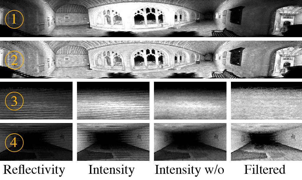
Figure 4: (1): The intensity image is over- (center) and under-exposed (sides). (2): Our filtered image has consistent brightness across the image. (3) & (4): Detail views from a grass field (3) and tunnel (4). The reflectivity image is under-exposed and does not show the ground markings (4). The intensity suffers from strong line artifacts that dominate the texture (3). Our filter removes the line artifacts (Intensity w/o). Our brightness compensation produces consistent exposure and shows details at larger range (ground markings in (4), grass texture in (3)).

III-E Geometrically Complementary Patch Selection

We select and track $5\times 5$ pixel patches which has shown better convergence compared to single pixels [23]. In contrast to prior works that select features randomly [21] or based on visual feature detectors [18, 19], we follow an approach inspired by [24]. We select candidate pixels with an image gradient magnitude above a threshold and perform a radius based non-maximum suppression. This approach does not rely on corner features which is favourable for low-texture images. Candidate pixels are mostly detected on shape discontinuities in the 3D scene such as edges and corners, or on changes in surface reflectivity, e.g. from ground markings or vegetation. The information from Jacobians from pixels on shape discontinuities often overlaps with the information that is already captured in the point-to-normal registration. We thus aim to select candidates that give additional information to efficiently leverage the multi-modality.

To detect uninformative directions in the point cloud registration, we follow the information analysis presented in X-ICP. We calculate the principal components of the Hessian ${\mathbf{H}^{geo}}^{T}\mathbf{H}^{geo}$ of the point-to-plane terms. A direction is then detected as uninformative if the accumulated filtered contribution is below a threshold. We refer the reader to [8] for more details. We analyze the translational components and denote the set of uninformative directions $\mathit{V}_{t}$. If all directions are informative, we insert vectors along the coordinate axes to promote equally distributed gradients.

We calculate the second image moment $M$ [25] and use its strongest eigenvector $\mathbf{v}_{patch}$ to approximate the patch gradient, which is more stable than pixel gradients. We then calculate how the projected image coordinate changes, if the point is perturbed along a direction using (7):

$$\mathbf{d}_{p_{i}}=\frac{\partial\Pi({}_{L_{j}}\mathbf{p}_{j})}{\partial{}_{L_{j}}\mathbf{p}_{j}}\cdot\mathbf{v}_{t,i}\in\mathbb{R}^{2},\,\forall\,\mathbf{v}_{t,i}\in V_{t}$$ (3)

We select features where shifting the point along an uninformative 3D direction results in a 2D coordinate shift in an informative image direction. We therefore project the projection gradient $\mathbf{d}_{p_{i}}$ onto the informative direction $\mathbf{v}_{patch}$ of the patch to calculate its directional contribution $c_{i}$. As the magnitude of the projection gradient increases with decreasing range, which would favour the selection of points close to the sensor, we use the normalized gradient instead:

$$c_{i}=\frac{\mathbf{d}_{p_{i}}\cdot\mathbf{v}_{patch}}{||\mathbf{d}_{p_{i}}||}$$ (4)

For each direction in $V_{t}$, we select the patches with the strongest contribution. We visualize the results in Figure 5.

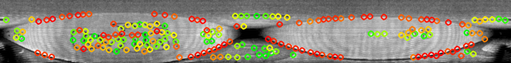
Figure 5: Top: Example frame. Bottom: Features are colored by contribution strength in the uninformative axis along the tunnel (increases from red to green). Uninformative features along the tunnel edges are correctly marked in red, while features with strong gradient along the tunnel show up green.

III-F Feature Management

We initialize each point in a patch separately at its global position using the current pose estimate and store the corresponding filtered intensity value. Differently from visual odometry approaches [23], where one position is assigned to the whole patch, this allows us to project each point in the patch separately. Using high resolution patches we can capture fine-grained details in contrast to prior works [21, 14] which only store a single value per voxel-grid cell. To keep the computational load bounded, we limit the number of tracked patches. After each update step, we asses the feature patch validity. To detect occlusions, we compare the predicted and measured range for each point in the patch and discard all points in it if the difference is above a threshold. We also remove patches if the measured range is below a minimum or above a maximum range. Additionally, we calculate the normalized cross correlation (NCC) between a tracked and measured patch and remove it if the NCC is below a threshold. We only track features over a maximum amount of frames to reduce error accumulation and to encourage initialization of new features. We avoid overlapping features and improve feature distribution by enforcing a minimum distance between new and tracked features.

III-G Photometric Residual & Kalman Update

We minimize photometric errors between tracked and currently observed points. The error is computed by projecting tracked points into the current image and comparing current intensity values to the patch:

$$z^{pho}=I_{c}(\Pi({}_{L_{j}}\mathbf{p}_{f}))-i_{f}\vspace{-1mm}$$ (5)

As rotating LiDARs record individual points sequentially, the pixels inside the intensity image are measured at different times and different poses. We project the position of the tracked point in the LiDAR frame $L_{j}$ at the time of the corresponding pixel:

$${}_{L_{j}}\mathbf{p}_{f}=\mathbf{T}_{L_{j}I_{j}}\mathbf{T}_{I_{j}I_{k}}\mathbf{T}_{I_{k}G}{}_{G}\mathbf{p}_{f}$$ (6)

However, this is dependent on $\mathbf{T}_{I_{j}I_{k}}$, which in turn depends on the unknown time $t_{j}$ itself. RI-LIO solves this by using a kNN-search in a kD-tree. However, this is only computationally feasible at a low resolution. We thus propose a projection-based solution. Given the undistorted point cloud, we can approximate which areas in the environment were captured at which timestamp. Therefore, we build an undistortion image by projecting the undistorted point cloud into an image and assign each pixel the index of the corresponding point: $\mathcal{U}(\Pi({}_{L_{k}}\mathbf{p}_{j}))=j$.

To find the corresponding index for the feature point, we then project it to the undistortion map, which is drastically cheaper than kD-tree-search and thus applicable to the full resolution point cloud. Given the index, we find the respective timestamp and $\mathbf{T}_{I_{j}I_{k}}$ to calculate (6) and finally (5).

The resulting Jacobian $\mathbf{H}^{pho}$ is calculated as:

$${\mathbf{H}^{pho}_{j}}=\frac{\partial\mathcal{I}[{}_{C}\mathbf{p}_{j}]}{\partial{}_{C}\mathbf{p}_{j}}\cdot\frac{\partial\Pi({}_{L_{j}}\mathbf{p}_{j})}{\partial{}_{L_{j}}\mathbf{p}_{j}}\cdot\frac{\partial{}_{L_{j}}\mathbf{p}_{j}}{\partial\tilde{\mathbf{x}}}$$ (7)

$$\frac{\partial\mathcal{I}[{}_{C}\mathbf{p}_{j}]}{\partial{}_{C}\mathbf{p}_{j}}=\begin{bmatrix}\frac{-f_{x}y}{x^{2}+y^{2}}&\frac{f_{x}x}{x^{2}+y^{2}}&0\\ -\frac{f_{y}xz}{LR^{2}}&-\frac{f_{y}yz}{LR^{2}}&\frac{f_{y}L}{R^{2}}\end{bmatrix}$$ (8)

$\frac{\partial\mathcal{I}[{}_{C}\mathbf{p}_{j}]}{\partial{}_{C}\mathbf{p}_{j}}$

is the image gradient from neighboring pixels.

We stack the point-to-plane (^geo) and photometric (^pho) terms into a combined residual vector ($\mathbf{z}$) and Jacobian ($\mathbf{H}$). The scaling factor $\sigma$ compensates for the different error magnitudes between geometric and photometric residuals:

$\mathbf{H}=\begin{bmatrix}{\mathbf{H}^{geo}_{1}}^{T},\cdot\cdot\cdot,{\mathbf{H}^{geo}_{m}}^{T},\lambda\cdot{\mathbf{H}^{pho}_{1}}^{T},\cdot\cdot\cdot,\lambda\cdot{\mathbf{H}^{pho}_{n}}^{T}\end{bmatrix}^{T}$ $\mathbf{z}_{k}^{\kappa}=\begin{bmatrix}{z^{geo}_{1}},\cdot\cdot\cdot,{z^{geo}_{m}},\lambda\cdot{z^{pho}_{1}},\cdot\cdot\cdot,\lambda\cdot{z^{pho}_{n}}\end{bmatrix}^{T}$ $\mathbf{R}=\text{diag}\begin{bmatrix}\sigma\end{bmatrix}\vspace{1mm}$

We use the formulas provided in [1] to update the state:

$$\mathbf{K}=(\mathbf{H}^{T}\mathbf{R}^{-1}\mathbf{H}+\mathbf{P}^{-1})^{-1}\mathbf{H}^{T}\mathbf{R}^{-1}$$ (10)

IV Experimental Results

We quantitatively compare our proposed pipeline with several state-of-the-art approaches as baselines: KISS-ICP [7], LIO-SAM [9] and FAST-LIO2 [1] represent widely used LO and LIO algorithms. Similar to our approach, MD-SLAM [20], Du [19] and RI-LIO [21] also use intensity or reflectivity information. We use the Newer College Dataset [26] as a public baseline. To evaluate robustness in low-structured environments, we additionally provide and evaluate on a new dataset of geometrically degenerate scenes that is presented in Section IV-A. We calculated the absolute translational error (ATE) and the relative translational error (RTE) over segments of 10m using the evo library [27]. We declare approaches with an RTE that is larger than $20\%$ as failed (indicated by $\times$) and do not report their ATE, as the required alignment between estimate and ground truth trajectories is not meaningful if the estimated trajectory differs too much from the ground truth. Apart from sensor extrinsics, calibrations and minimum range (to adapt for narrow scenes), we used the default parameters that were provided by the baseline approaches. We slightly increased the reflectivity covariance parameter in RI-LIO, as the default value caused divergence in all tested sequences.

IV-A ENWIDE Dataset

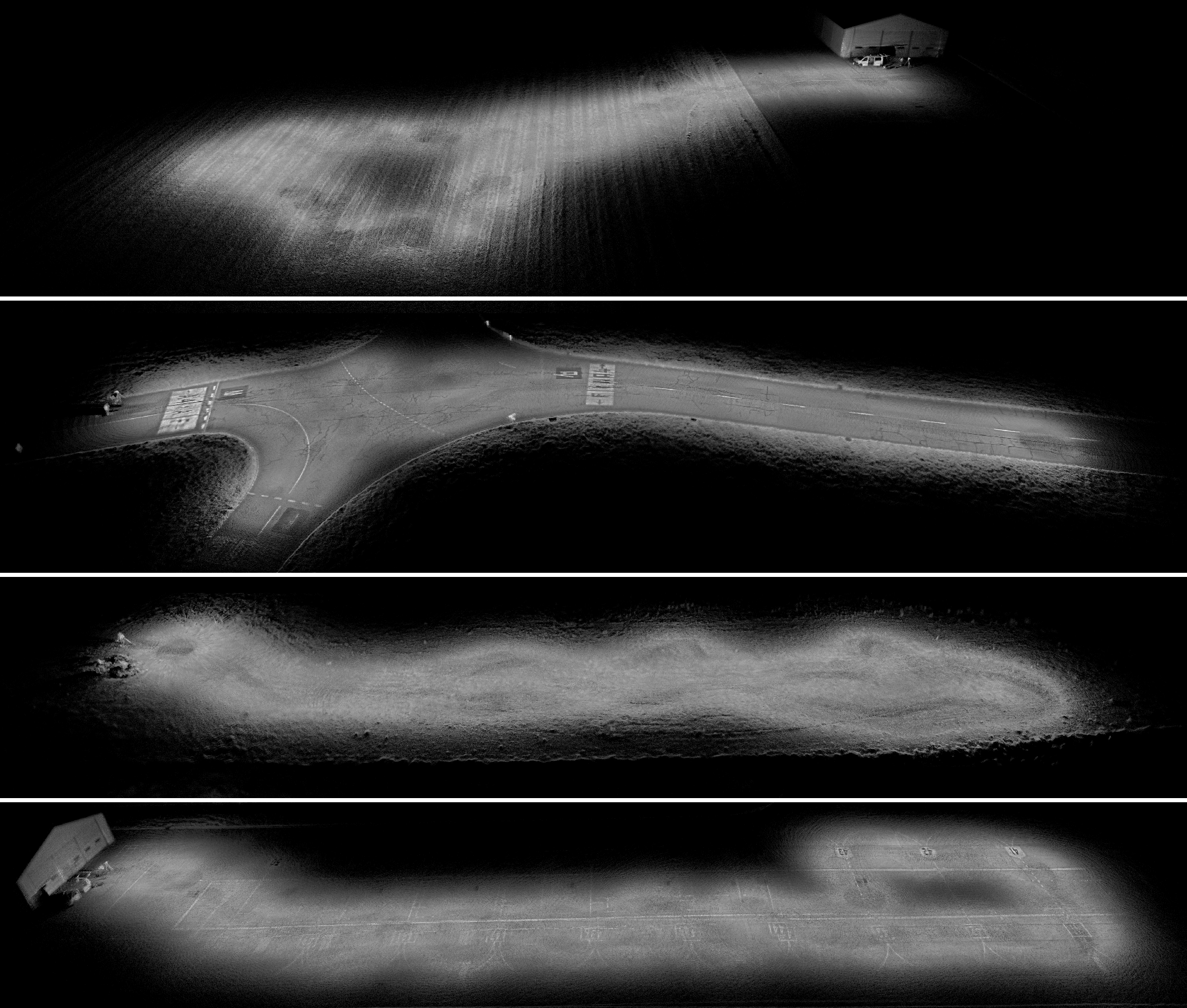
Figure 6: Resulting maps from COIN-LIO on the ENWIDE dataset. Top to bottom: FieldS, IntersectionS, KatzenseeS, RunwayS. Despite long degenerate sections, COIN-LIO produces consistent, sharp maps.

As geometrically degenerate environments are barely represented in existing open-sourced datasets, we created a new dataset with long segments of real-world geometric degeneracy (Fig. 6). Using a hand-held Ouster OS0 128 beam LiDAR with integrated IMU, we recorded five distinct environments: Tunnel (urban, indoor), Intersection (urban, outdoor), Runway (outdoor, urban), Field (outdoor, nature), Katzensee (outdoor, nature). All sequences contain long sections of geometric degeneracy, but start and end in well-constrained areas. Tunnel/Intersection/Runway sequences contain strong intensity features, Katzensee/Field contain few salient features. For each environment we provide one smooth (walking, slow motions, e.g. FieldS) and one dynamic (running, aggressive motions, e.g. FieldD) sequence. Ground truth positions were recorded from a Leica MS60 station at 20 Hz (interpolated to 200Hz) with approximately 3cm accuracy.

TABLE I: Newer College Dataset
Absolute Trajectory Error (m) / Relative Error (%)

max width= Method Quad-Hard Cloister Stairs Park Length (m) $234.81$ $428.79$ $57.04$ $2396.20$ KISS-ICP [7] $0.324$ / $1.88$ $0.297$ / $2.07$ $\times$ / $32.48$ $2.871$ / $1.06$ MD-SLAM [20] $19.639$ / $12.36$ $0.360$ / $2.73$ $0.340$ / $6.21$ $96.797$ / $23.03$ Du and Beltrame [19] $18.506$ / $16.432$ $59.544$ / $19.274$ $\times$ / $26.121$ $\times$ / $42.717$ LIO-SAM [9] $0.299$ / $2.380$ $0.145$ / $1.032$ $\times$ / $5122.320$ $1.566$ / $2.064$ FAST-LIO2 [1] $0.049$ / $\mathbf{0.26}$ $\mathbf{0.078}$ / $\mathbf{0.23}$ $\times$ / $3497.22$ $0.310$ / $0.59$ RI-LIO [21] $0.237$ / $1.04$ $0.285$ / $1.33$ $\times$ / $16877.28$ $89.289$ / $5.00$ Ours $\mathbf{0.046}$ / $0.29$ $\mathbf{0.078}$ / $0.28$ $\mathbf{0.102}$ / $\mathbf{0.74}$ $\mathbf{0.287}$ / $\mathbf{0.54}$

TABLE II: ENWIDE Dataset - Absolute Trajectory Error (m) / Relative Error (%)

max width= Method TunnelS TunnelD IntersectionS IntersectionD RunwayS RunwayD FieldS FieldD KatzenseeS KatzenseeD Length (m) $251.58$ $179.71$ $279.28$ $388.47$ $333.57$ $357.14$ $232.70$ $287.91$ $242.88$ $177.20$ KISS-ICP [7] $\times$ / $144.41$ $\times$ / $68.11$ $\times$ / $65.69$ $\times$ / $64.84$ $\times$ / $113.45$ $\times$ / $124.64$ $\times$ / $54.84$ $\times$ / $70.70$ $\times$ / $66.23$ $\times$ / $76.80$ MD-SLAM [20] $\times$ / $88.16$ $\times$ / $80.76$ $\times$ / $90.87$ $\times$ / $87.89$ $\times$ / $97.73$ $\times$ / $91.13$ $\times$ / $96.03$ $\times$ / $84.86$ $\times$ / $93.92$ $\times$ / $91.29$ Du and Beltrame [19] $\times$ / $58.084$ $\times$ / $56.086$ $\times$ / $60.812$ $\times$ / $57.449$ $\times$ / $67.906$ $\times$ / $63.978$ $\times$ / $72.548$ $\times$ / $69.480$ $\times$ / $93.92$ $\times$ / $74.207$ LIO-SAM [9] $\times$ / $2565.621$ $\times$ / $2662.983$ $\times$ / $2022.878$ $\times$ / $2362.314$ $\times$ / $2334.174$ $\times$ / $3984.588$ $\times$ / $2196.344$ $\times$ / $1999.968$ $5.588$ / $2.673$ $\times$ / $1485.377$ FAST-LIO2 [1] $\times$ / $316.12$ $\times$ / $81.31$ $12.473$ / $29.28$ $23.800$ / $28.11$ $\times$ / $53.64$ $\times$ / $59.84$ $\mathbf{0.163}$ / $\mathbf{0.57}$ $9.209$ / $16.08$ $1.122$ / $4.31$ $1.02$ / $2.38$ RI-LIO [21] $\times$ / $70.32$ $\times$ / $63.02$ $\times$ / $49.94$ $\times$ / $188.83$ $\times$ / $52.18$ $\times$ / $79.16$ $1.721$ / $2.44$ $24.851$ / $25.89$ $\times$ / $49.34$ $\times$ / $154.19$ Ours $\mathbf{0.743}$ / $\mathbf{1.60}$ $\mathbf{0.487}$ / $\mathbf{1.59}$ $\mathbf{0.466}$ / $\mathbf{1.25}$ $\mathbf{1.912}$ / $\mathbf{1.69}$ $\mathbf{1.033}$ / $\mathbf{1.89}$ $\mathbf{2.437}$ / $\mathbf{2.98}$ $0.232$ / $0.85$ $\mathbf{0.581}$ / $\mathbf{1.83}$ $\mathbf{0.412}$ / $\mathbf{0.99}$ $\mathbf{0.592}$ / $\mathbf{1.61}$

IV-B Newer College Results

The Newer College Dataset [26] uses a hand-held 128-beam Ouster OS0. We present the results in Table I. In the Cloister sequence, which contains large structures and slow motions, all tested approaches achieve a low ATE. In Quad-Hard, aggressive rotations occur. Due to the absence of an ego-motion compensation, the LO approaches perform worst. Our approach achieves the lowest ATE, which confirms that our computationally-cheap image motion-compensation method is effective. The Stairs sequence causes several approaches to diverge, as they use heavy spatial-downsampling of the point cloud to achieve real-time performance, which in the case of this narrow stairway removes too much information. While our approach uses the same downsampling for the geometric part, it achieves robust and accurate performance thanks to the photometric component. This unveils an inherent benefit of image-based intensity augmentation: fixed-size patches in the image implicitly capture different amounts of volume depending on the point distance. Thereby, projected images have automatic adaptive resolution at a constant cost, contrary to the increased cost resulting from a higher voxel-resolution necessary to capture the same information. While RI-LIO uses information from reflectivity images, its random feature selection fails to extract salient information and therefore diverges. In contrast, the dense approach in MD-SLAM does not fail, but is outperformed by our approach. We perform slightly better than FAST-LIO2 on the significantly longer but geometry-rich Park dataset, showing that the intensity features can also improve performance in non-degenerate scenarios. We also evaluate our runtime on the Park sequence which is the longest in our experiments. On average, our approach consumes 29.7ms per frame (33 Hz) on an Intel i7-11800H mobile CPU, of which only 6.2ms are spent on the photometric components, which shows that the main computational cost results from the conventional geometric approach.

IV-C ENWIDE Results

While our approach showed improved accuracy in Table I, the main motivation behind this work is to leverage intensity to improve robustness of LIO in challenging scenarios. We therefore evaluate on the challenging ENWIDE Dataset, presented in Table II. It is plausible, that KISS-ICP fails in all sequences as it only operates on the (degenerate) point cloud geometry. However, we observe that MD-SLAM and Du, which also leverage the intensity channel, diverge in all sequences too. Both do not use the IMU, unlike LIO approaches, which impacts their ability to handle even short segments of geometric degeneracy or fast rotations. Additionally, Du only uses the images for geometric feature selection, and cannot benefit from additional texture information in the optimization. Despite using reflectivity and IMU, RI-LIO diverged in most sequences, which we discuss below.

Due to noise in the IMU measurements and drifting biases, LIO approaches can still fail in longer segments of geometric degeneracy. This is evident in LIO-SAM, which uses curvature-based point cloud features [6]. FAST-LIO2, which operates on points directly, is able to avoid a failure in (Intersection, Field, Katzensee) where the present vegetation still offers some weak information, but exhibits large drift. However, we observe a failure in man-made environments (Tunnel, Runway), where the geometry is effectively perfectly degenerate. Despite this, our approach achieves robust performance in all tested sequences, by leveraging the complementary information provided by the photometric error minimization. While we consider the increased robustness in scenarios where prior approaches fail as the main strength of our approach, we also note our higher accuracy than FAST-LIO2 on most successful sequences. The main limitation of our approach is the dependence on specific high-resolution LiDARs that create dense intensity images.

IV-D Ablation study

We show the effects of our image processing and feature selection decisions in Table III. We compare the proposed Filtered image with Intensity and Reflectivity images. We also evaluate different feature selection policies by comparing Random (similar to RI-LIO [21]) as well as Strongest image gradient selection with the proposed geometrically Complementary selection. We note lower error from (Intensity, Strongest) than (Reflectivity, Strongest). This seems surprising at first, as the reflectivity value compensates the range dependency of the signal. However, we observed that the reflectivity image contains stronger noise and artifacts and has less consistent brightness across the image. Our proposed image processing (Filtered, Strongest) improves performance in low textured environments (TunnelD, KatzenseeD). There, the line artifacts are more dominant than the actual features from the environment. Additionally, the brightness decreases drastically with increasing range. In contrast, the brightness compensation and line removal of our filtered image allows to use more fine-grained details, e.g. from vegetation or gravel, at larger range. We note that (Intensity, Strongest) marginally outperforms (Filtered, Strongest) on IntersectionS. In this scene, strong image features from road cracks are consistently found at short range. We believe that the slightly lower ATE results the filtered image having lower contrast than the intensity image at short range in this scene, which results in weaker gradients. Selecting features based on strong image gradients (Filtered, Strong) results in better performance compared to random patches (Filtered, Random), as they provide richer information for the filter updates. Our proposed feature selection scheme (Filtered, Complementary) achieves the highest performance, as it reduces redundant information along uninformative geometric directions and specifically selects informative image patches. It can be noted that its impact is strongest in TunnelD, where most strong gradients are in the geometrically degenerate direction along the tunnel (see Figure 5, while they are more randomly oriented in the other scenes. Overall, the ablation experiments confirm that COIN-LIO is able to effectively leverage the additional information provided by the multi-modality of the approach.

TABLE III: Ablation Study - Absolute Trajectory Error (RMSE) (m)

Image	Features	TunnelD	IntersectionS	KatzenseeD
Intensity	Strongest	$13.928$	$0.472$	$0.948$
Reflectivity	Strongest	$\times$	$0.699$	$0.874$
Filtered	Strongest	$0.814$	$0.489$	$0.701$
Filtered	Random	$1.913$	$0.580$	$1.073$
Filtered	Complementary	$\mathbf{0.487}$	$\mathbf{0.466}$	$\mathbf{0.592}$

V Conclusion

This work proposed COIN-LIO, a framework that tightly fuses photometric error minimization for improved robustness in geometrically degenerate environments. We presented an image pipeline to produce brightness compensated intensity images that provide more fine-grained details at larger range and consistent illumination across different environments. Our novel feature selection scheme effectively leverages the multi-modality by providing additional instead of redundant information. Our approach slightly outperforms baseline approaches on the geometry-rich Newer College Dataset, and shows drastically increased robustness in our geometrically-degenerate ENWIDE dataset, which enables benchmarking LIO in previously underrepresented scenarios.

We believe that this dataset as well as our work serve as a motivation for a new line of research that shifts from chasing even higher accuracies in geometrically simple cases to improving robustness in challenging environments. We also hope it motivates the industry to further improve the imaging capabilities of LiDAR.

References

- [1] Wei Xu et al. “Fast-lio2: Fast direct lidar-inertial odometry”, 2022, pp. 2053–2073
- [2] Ji Zhang and Sanjiv Singh “Laser–visual–inertial odometry and mapping with high robustness and low drift” In Journal of field robotics 35.8 Wiley Online Library, 2018, pp. 1242–1264
- [3] Xingxing Zuo et al. “Lic-fusion 2.0: Lidar-inertial-camera odometry with sliding-window plane-feature tracking” In 2020 IEEE/RSJ International Conference on Intelligent Robots and Systems (IROS), 2020, pp. 5112–5119 IEEE
- [4] David Wisth, Marco Camurri and Maurice Fallon “VILENS: Visual, inertial, lidar, and leg odometry for all-terrain legged robots” In IEEE Transactions on Robotics IEEE, 2022
- [5] Jiarong Lin and Fu Zhang “R3LIVE: A Robust, Real-time, RGB-colored, LiDAR-Inertial-Visual tightly-coupled state Estimation and mapping package” In 2022 International Conference on Robotics and Automation (ICRA), 2022, pp. 10672–10678
- [6] Ji Zhang and Sanjiv Singh “LOAM: Lidar odometry and mapping in real-time.” In Robotics: Science and systems 2.9, 2014, pp. 1–9 Berkeley, CA
- [7] Ignacio Vizzo et al. “KISS-ICP: In Defense of Point-to-Point ICP – Simple, Accurate, and Robust Registration If Done the Right Way” In IEEE Robotics and Automation Letters 8.2, 2023, pp. 1029–1036
- [8] Turcan Tuna et al. “X-ICP: Localizability-Aware LiDAR Registration for Robust Localization in Extreme Environments”, 2023 arXiv:2211.16335 [cs.RO]
- [9] Tixiao Shan et al. “LIO-SAM: Tightly-coupled Lidar Inertial Odometry via Smoothing and Mapping” In 2020 IEEE/RSJ International Conference on Intelligent Robots and Systems (IROS), 2020, pp. 5135–5142
- [10] Michael Kaess et al. “iSAM2: Incremental smoothing and mapping with fluid relinearization and incremental variable reordering” In 2011 IEEE International Conference on Robotics and Automation, 2011, pp. 3281–3288
- [11] Frank Dellaert and Michael Kaess “Factor Graphs for Robot Perception” In Found. Trends Robotics 6, 2017, pp. 1–139
- [12] Wei Xu and Fu Zhang “FAST-LIO: A Fast, Robust LiDAR-Inertial Odometry Package by Tightly-Coupled Iterated Kalman Filter” In IEEE Robotics and Automation Letters 6.2, 2021, pp. 3317–3324
- [13] Yeong Sang Park, Hyesu Jang and Ayoung Kim “I-LOAM: Intensity Enhanced LiDAR Odometry and Mapping” In 2020 17th International Conference on Ubiquitous Robots (UR), 2020, pp. 455–458
- [14] H. Wang, C. Wang and L. Xie “Intensity-SLAM: Intensity Assisted Localization and Mapping for Large Scale Environment” In IEEE Robotics and Automation Letters 6.2, 2021, pp. 1715–1721
- [15] Haisong Li, Bailing Tian, Hongming Shen and Junjie Lu “An Intensity-Augmented LiDAR-Inertial SLAM for Solid-State LiDARs in Degenerated Environments” In IEEE Transactions on Instrumentation and Measurement 71, 2022, pp. 1–10
- [16] Shuaixin Li et al. “InTEn-LOAM: Intensity and Temporal Enhanced LiDAR Odometry and Mapping” In Remote Sensing 15.1, 2023
- [17] Yue Pan et al. “MULLS: Versatile LiDAR SLAM via Multi-metric Linear Least Square” In 2021 IEEE International Conference on Robotics and Automation (ICRA), 2021, pp. 11633–11640
- [18] Tiziano Guadagnino et al. “Fast Sparse LiDAR Odometry Using Self-Supervised Feature Selection on Intensity Images” In IEEE Robotics and Automation Letters 7.3, 2022, pp. 7597–7604
- [19] Wenqiang Du and Giovanni Beltrame “Real-Time Simultaneous Localization and Mapping with LiDAR Intensity” In 2023 IEEE International Conference on Robotics and Automation (ICRA), 2023, pp. 4164–4170
- [20] Luca Di Giammarino et al. “MD-SLAM: Multi-cue Direct SLAM” In 2022 IEEE/RSJ International Conference on Intelligent Robots and Systems (IROS), 2022, pp. 11047–11054
- [21] Yanfeng Zhang et al. “RI-LIO: Reflectivity Image Assisted Tightly-Coupled LiDAR-Inertial Odometry” In IEEE Robotics and Automation Letters 8.3, 2023, pp. 1802–1809
- [22] Dongjiao He, Wei Xu and Fu Zhang “Kalman filters on differentiable manifolds” In arXiv preprint arXiv:2102.03804, 2021
- [23] Christian Forster et al. “SVO: Semidirect Visual Odometry for Monocular and Multicamera Systems” In IEEE Transactions on Robotics 33.2, 2017, pp. 249–265
- [24] Jakob Engel, Vladlen Koltun and Daniel Cremers “Direct sparse odometry” In IEEE transactions on pattern analysis and machine intelligence 40.3 IEEE, 2017, pp. 611–625
- [25] Chris Harris and Mike Stephens “A combined corner and edge detector” In Alvey vision conference 15.50, 1988, pp. 10–5244 Citeseer
- [26] Lintong Zhang, Marco Camurri, David Wisth and Maurice Fallon “Multi-camera lidar inertial extension to the newer college dataset” In arXiv preprint arXiv:2112.08854, 2021
- [27] Michael Grupp “evo: Python package for the evaluation of odometry and SLAM.”, 2017