From Bricks to Bridges: Product of Invariances
to Enhance Latent Space Communication

Abstract

It has been observed that representations learned by distinct neural networks conceal structural similarities when the models are trained under similar inductive biases. From a geometric perspective, identifying the classes of transformations and the related invariances that connect these representations is fundamental to unlocking applications, such as merging, stitching, and reusing different neural modules. However, estimating task-specific transformations a priori can be challenging and expensive due to several factors (e.g., weights initialization, training hyperparameters, or data modality). To this end, we introduce a versatile method to directly incorporate a set of invariances into the representations, constructing a product space of invariant components on top of the latent representations without requiring prior knowledge about the optimal invariance to infuse. We validate our solution on classification and reconstruction tasks, observing consistent latent similarity and downstream performance improvements in a zero-shot stitching setting. The experimental analysis comprises three modalities (vision, text, and graphs), twelve pretrained foundational models, eight benchmarks, and several architectures trained from scratch.

1 Introduction

Discovering symmetries and conserved quantities is a core step for extracting meaningful representations from raw data in biological and artificial systems Higgins et al. (2022); Benton et al. (2020);

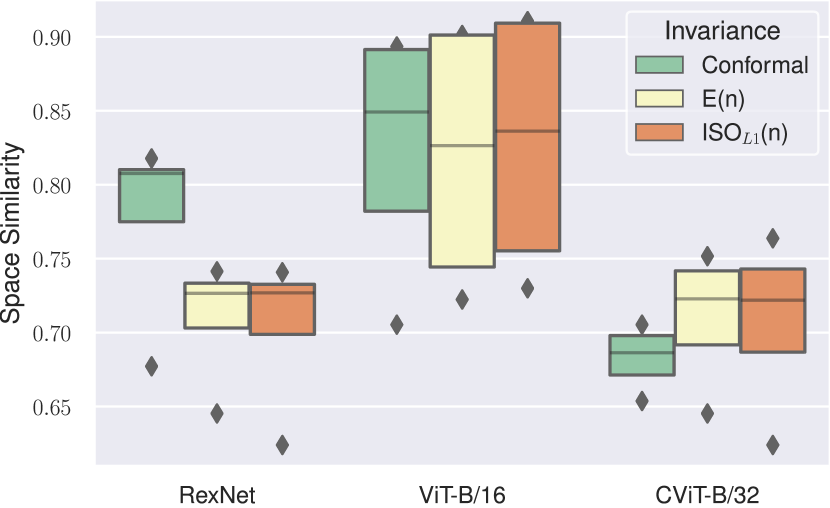
Figure 1: CKA similarity (Kornblith et al. (2019)) of pretrained models on F-MNIST, measured on projections of the latent space onto subspaces invariant to specific classes of transformations (Conformal, Euclidean, Orthogonal). In each bar, we report the distribution of similarity to the other models, while infusing a specific invariance. The score diversity highlights the absence of a universal transformation connecting all latent spaces.

Lyle et al. (2020). Achieving invariance to specific groups of transformations within neural models holds significant utility in a wide range of real-world applications, such as comparing similar latent spaces across multiple training instances, facilitating communication, and enabling model reuse Cohen & Welling (2016); Fawzi et al. (2016); Salamon & Bello (2017); Klabunde et al. (2023). These desired invariances can be defined with respect to transformations in the input space Benton et al. (2020); Immer et al. (2022); Cohen & Welling (2016); Cohen et al. (2019), or in relation to the latent space, as explored by Moschella et al. (2022). Such properties can arise implicitly from architectural choices Cohen & Welling (2016); Cohen et al. (2019); Worrall et al. (2017); Zhou et al. (2017) or be explicitly enforced using methods like loss penalties Arjovsky et al. (2019). A recent study introduced the concept of Relative Representation (RR) Moschella et al. (2022). In its original formulation, this framework enforces invariance to angle-preserving transformations of the latent space. This approach enhances communication between latent spaces by projecting them into a shared relative space determined by distances between data points. However, as shown in Figure 1, the transformations relating different neural representations are not always consistent with a single class of transformations, such as the one considered in Moschella et al. (2022). Determining a priori which class of transformations relates distinct latent spaces is challenging due to complex interactions in the data, and multiple nuisance factors that are typically irrelevant but can nevertheless affect the representation (e.g. random initialization, neural architecture, and data modality). To address this challenge, we expand upon the method of RR, presenting a framework to efficiently incorporate a set of invariances into the learned latent space. This is achieved by constructing a product space of invariant components on top of the latent representations of, possibly pretrained, neural models. Each component of this product space is obtained by projecting samples as a function of fixed data points, denoted as anchors. Using different similarity functions for each subspace, we can infuse invariances to specific transformations into each component of the product space. Our main contributions can be summarized as follows:

• We show that the class of transformation that relates representations learned by distinct Neural Networks (NNs)–trained on semantically similar data–may vary and depends on multiple factors;

• We introduce a framework for infusing multiple invariances into a single latent representation, constructing a product space of invariant components to enhance latent communication;

• We validate our findings on stitching tasks across various data modalities, including images, text, and graphs: product of invariances can capture arbitrary complex transformations of the latent space in a single representation, achieving the best performance without any prior knowledge of the transformation or the factors that may affect it.

2 Related work

Representation Similarity. Several metrics have been proposed to compare latent spaces generated by independent NNs, capturing their inherent similarity up to transformations that correlate the spaces. A classical statistical method is Canonical Correlation Analysis (CCA) Hotelling (1992), which is invariant to linear transformations. While variations of CCA seek to improve robustness through techniques like Singular Value Decomposition (SVD) and Singular Value CCA (SVCCA) Raghu et al. (2017) or to reduce sensitivity to perturbations using methods such as Projection Weighted CCA (PWCCA) Morcos et al. (2018). Closely related to these metrics, the Centered Kernel Alignment (CKA) metric Kornblith et al. (2019) measures the similarity between latent spaces while disregarding orthogonal transformations. However, recent research Davari et al. (2022) demonstrates its sensitivity to transformations that shift a subset of data points in the representation space.

Learning and Incorporating Invariance and Equivariance into Representations. Invariances in NN models can be enforced through various techniques operating at different levels, including adjustments to model architecture, training constraints, or input manipulation Lyle et al. (2020). Benton et al. (2020) proposes a method to learn invariances and equivariances, Immer et al. (2022) introduces a gradient-based approach that effectively captures inherent invariances in the data. Meanwhile, van der Ouderaa & van der Wilk (2022) enables training of NNs with invariance to specific transformations by learning weight-space equivalents instead of modifying the input data. Other works directly incorporate invariances into the model through specific constraints. Rath & Condurache (2023) enforces a multi-stream architecture to exhibit invariance to various symmetry transformations without relying on data-driven learning, Kandi et al. (2019) propose an improved Convolutional Neural Network (CNN) architecture for better rotation invariance, and Gandikota et al. (2021) introduces a method for designing network architectures that are invariant or equivariant to structured transformations. Finally, Moschella et al. (2022) proposes an alternative representation of the latent space that guarantees invariance to angle-preserving transformation without requiring additional training but only a set of anchors, possibly very small (Cannistraci et al., 2023).

Our work leverages the RR framework to directly incorporate a set of invariances into the learned latent space, creating a product space of invariant components which, combined, can capture arbitrary complex transformations of the latent space.

3 Infusing invariances

\begin{overpic}[trim=0.0pt 0.0pt 0.0pt 0.0pt,clip,tics=5,width=271.0125pt]{images/3.method/latentin-manifold.drawio.pdf} \put(-5.0,33.5){$\mathcal{X}$} \put(-5.0,9.5){$\mathcal{X}$} \put(3.0,33.5){$E$} \put(3.0,9.5){$E^{\prime}$} \put(27.0,20.5){$T$} \put(16.0,20.5){$T^{-1}$} \put(16.75,38.0){$\mathcal{Z}$} \put(16.0,2.0){$\mathcal{Z}^{\prime}$} \put(49.5,20.5){$\mathcal{M}\approx\tilde{\mathcal{M}}$} \put(75.5,20.5){$r\approx\pi_{\mathcal{M}}$} \put(32.0,20.5){$\pi_{\mathcal{M}}$} \put(38.0,35.5){Relative representations} \put(38.0,6.0){Relative representations} \end{overpic}

Figure 2: Framework description. Given two latent spaces $\mathcal{Z},\mathcal{Z}^{\prime}$ related by an unknown transformation $T$ (resp. $T^{-1}$), we assume that there exist a manifold $\mathcal{M}$ where samples in $\mathcal{Z},\mathcal{Z}^{\prime}$ coincides when projected into $\mathcal{M}$, via $\pi_{\mathcal{M}}$. We approximate $\mathcal{M}$ building a product space $\tilde{\mathcal{M}}$, where each subspace is a relative representation computed using a similarity function $d_{i}$ invariant to a specific, known class of transformations. By combing the resulting set of invariances we recover a representation $r$ which should approximate $\pi_{\mathcal{M}}$.

Setting. We consider neural networks as parametric functions $F_{\theta}$ compositions of encoding and decoding maps $F_{\theta}=D_{\theta_{2}}\circ E_{\theta_{1}}$, where the encoder $E_{\theta_{1}}$ is responsible for computing a latent representation $z=E_{\theta_{1}}(x),\ \ x\in\mathcal{X}$ for some domain $\mathcal{X}$, with $dim(\mathcal{Z})<<dim(\mathcal{X})$; and the decoder $D_{\theta_{2}}$ is responsible for solving the task at hand (e.g., reconstruction, generation, classification). In the following, we will drop the dependence on parameters $\theta$ for notational convenience. For a single module $E$ (equivalently for $D$), we indicate with $E_{\mathcal{X}}$ if the module $E$ was trained on the domain $\mathcal{X}$. In the upcoming, we summarize the necessary background to introduce our method.

Background. The RR framework Moschella et al. (2022) provides a straightforward approach to represent each sample in the latent space according to its similarity to a set of fixed training samples, denoted as anchors. Representing samples in the latent space as a function of the anchors corresponds to transitioning from an absolute coordinate frame into a relative one defined by the anchors and the similarity function. Given a domain $\mathcal{X}$, an encoding function $E_{\mathcal{X}}:\mathcal{X}\to\mathcal{Z}$, a set of anchors $\mathcal{A}_{\mathcal{X}}\subset\mathcal{X}$, and a similarity or distance function $d:\mathcal{Z}\times\mathcal{Z}\to\mathbb{R}$. The RR for each sample $x\in\mathcal{X}$ is computed as:

$$\lx@glossaries@gls@link{acronym}{rr}{\leavevmode RR}(z;\mathcal{A}_{\mathcal{X}},d)=\bigoplus_{a_{i}\in\mathcal{A}}d(z,a_{i})$$ (1)

where $z=E_{\mathcal{X}}(x)$, and $\bigoplus$ denotes row-wise concatenation. In Moschella et al. (2022), $d$ was set as cosine similarity. This choice induces a relative representation invariant to angle-preserving transformations. In this work, our focus is to leverage different choices of the similarity function to induce a set of invariances into the representations to capture arbitrarily complex transformations between latent spaces.

Overview. When considering different networks $F,F^{\prime}$, we are interested in modeling the class of transformations $\mathcal{T}$ that relates their latent spaces $\mathcal{Z},\mathcal{Z}^{\prime}$. $\mathcal{T}$ could be something known, e.g., rotations, or an arbitrary complex class of transformations.The two networks could differ by their initialization seeds (i.e., training dynamics), by architectural changes, or even domain changes, i.e., $\mathcal{X}\neq\mathcal{X}^{\prime}$, which could affect the latent space in a different way (as observed in Figure 1). The fundamental assumption of this work is that these variations induce changes in the latent representations of the models, but there exists an underlying manifold $\mathcal{M}$ where the representations are the same (see Figure 2). Formally:

Assumption.

Given multiple models $\mathcal{F}_{1}..\mathcal{F}_{n}$ we assume that there exists a manifold $\mathcal{M}$ which identifies an equivalence class of encoders $\mathcal{E}_{\mathcal{T}}$ induced by the class of transformation $\mathcal{T}$ (e.g. rotations), defined as $\mathcal{E}_{\mathcal{T}}:=\left\{E\ \ |\ \ \ \pi_{\mathcal{M}}TE=\pi_{\mathcal{M}}E,\ \ \ \forall T\in\mathcal{T}\right\}$, where $\pi_{\mathcal{M}}$ represent the projection on $\mathcal{M}$. $\mathcal{M}$ is equipped with a metric $d_{\mathcal{M}}$ which is preserved under the action of elements of $\mathcal{T}$, i.e. $d_{\mathcal{M}}(\pi_{\mathcal{M}}z,\pi_{\mathcal{M}}z^{\prime})=d_{\mathcal{M}}(\pi_{\mathcal{M}}T(z),\pi_{\mathcal{M}}T(z^{\prime}))$, $\forall T\in\mathcal{T}$

What we look for is a function $r$ which independently projects the latent spaces $\mathcal{Z}_{1}..\mathcal{Z}_{n}$ into $\mathcal{M}$ and is invariant to $\mathcal{T}$, i.e. $r(z)=r(Tz)$, for each $T\in\mathcal{T}$, and for each $z\in\mathcal{Z}_{1}..\mathcal{Z}_{n}$. Generalizing the framework of Moschella et al. (2022) to arbitrary similarity functions, or distance metrics, gives us a straightforward way to define representations $r$ invariant to specific classes of transformations.

However, $d_{\mathcal{M}}$ is typically unknown a priori, and in general, it is challenging to capture $\mathcal{T}$ with a single class of transformations (as observed in Figure 1and demonstrated in Section 4.1). To overcome this, in this work, we approximate $\mathcal{M}$ with a product space $\tilde{\mathcal{M}}:=\prod_{i=1}^{N}\mathcal{M}_{i}$, where each component is obtained by projecting samples of $\mathcal{Z}$ in a relative representation space equipped with a different similarity function $d_{i}$. Each $\mathcal{M}_{i}$ will have properties induced by a similarity function $d_{i}$ invariant to a specific, known, class of transformations $\tilde{\mathcal{T}_{i}}$ (e.g. dilations). By combining this set of invariances, we want to recover the representation $r$ such that it approximates well $\pi_{\mathcal{M}}$ (see Figure 2). We define $r$ formally as the projection from $\mathcal{Z}$ to $\tilde{\mathcal{M}}$:

Definition (Product projection).

Given a set of latent spaces $\mathcal{Z}_{1}..\mathcal{Z}_{n}$, related to one another by an unknown class of transformation $\mathcal{T}$, a set of similarity functions $\mathcal{D}$ each one invariant to a specific known class of transformations $\tilde{\mathcal{T}_{i}}$ (e.g. rotations), i.e. $RR(z,d_{i})=RR(Tz,d_{i})$, $\forall T\in\tilde{\mathcal{T}}_{i}$. We define the product projection $r:\mathcal{Z}\mapsto\tilde{\mathcal{M}}$ as:

$$r(z)=\phi\circ RR(z;\mathcal{A}_{\mathcal{X}},d_{i}),\ \ \ \ \ \forall d_{i}\in\mathcal{D}$$

where $\phi$ is an aggregation function (e.g. concatenation) responsible to merge the relative spaces induced by each $d_{i}\in\mathcal{D}$.

We give more details on different strategies on how to implement $\phi$ in section Definition.

Distance-induced invariances. We leverage the RR framework considering the following similarity functions $d$: Cosine (Cos.), Euclidean (Eucl.), Manhattan (L1), Chebyshev ($L_{\infty}$), and Geodesic (Geod.), each one inducing invariances to a specific, known class of transformations. For formal definitions, synthetic examples, and visualizations, please refer to the Section A.1.

Aggregation functions. This section summarizes different strategies to construct the product space $\tilde{\mathcal{M}}$, directly integrating a set of invariances into the representations. Consider a latent space $\mathcal{Z}$ image of an encoder $E:\mathcal{X}\mapsto\mathcal{Z}$, and a set of similarity functions $\mathcal{D}$. For each d $\in\mathcal{D}$, we produce $n=|\mathcal{D}|$ relative latent spaces. Every subspace is produced via a similarity function (i.e., Cos., Eucl., L1, or $L_{\infty}$), enforcing invariance to a specific class of transformations.

These subspaces can be merged using diverse aggregation strategies, corresponding to different choices of $\phi$:

• Concatenation (Concat): the subspaces are independently normalized and concatenated, giving to $\tilde{\mathcal{M}}$ the structure of a cartesian product space.

• Aggregation by sum (Sum): the subspaces are independently normalized and non-linearly projected. The resulting components are summed.

• Self-attention (SelfAttention): the subspaces are independently normalized and aggregated via a self-attention layer.

For the implementation details of each strategy, please refer to the Section A.3. The product space $\mathcal{M}$ yields a robust latent representation, made of invariant components which are combined to capture arbitrary complex transformations, boosting the performance on downstream tasks.

4 Experiments

In this section, we perform qualitative and quantitative experiments to analyze the effectiveness of our framework in constructing representations that can capture arbitrary complex transformations of the latent space. Specifically, Section 4.1 provides empirical motivation, analyzing how the similarity between latent spaces produced by AutoEncoder (AE) and Variational AutoEncoder (VAE) architectures, trained from scratch on various vision datasets may vary, according to the invariance enforced on the representation. Similar findings are presented by examining latent spaces generated by different pretrained models on multiple datasets and modalities (i.e., vision and text). Section 4.2 evaluates the zero-shot stitching performance of our aggregation framework across various modalities (i.e., text, vision, and graphs); Section 4.3 presents an ablation study on different aggregation functions. Finally, Section 4.4 focuses on the interpretability of our framework, examining attention weights and their role in selecting the optimal relative subspace.

4.1 Latent space analysis

Training from scratch

Experimental setting. In this experiment, we perform an image reconstruction task on CIFAR$-$10, CIFAR$-$100 (Krizhevsky et al., 2009), MNIST (Deng, 2012), and FashionMNIST (Xiao et al., 2017) datasets (refer to Table 8 for additional information). Using comparable convolutional architectures, we focus on AEs and VAEs. We consider models with an unflattened latent image bottleneck (referred to as AE and VAE) that preserve the image spatial structure and models with linear projections into and out of a flattened latent space (referred to as Linearized AutoEncoder (LinAE) and Linearized Variational AutoEncoder (LinVAE)). We train until convergence five instances for each combination, using different random seeds. Then, for each model, we project the latent spaces into their relative counterpart with different projection functions, thus infusing different invariances in each representation, and measure the latent space similarity across seeds for each combination.

\begin{overpic}[trim=0.0pt 0.0pt 0.0pt 0.0pt,clip,width=205.97214pt]{images/4.experiment/from_scratch/mnist_pearson_mean.pdf} \end{overpic}

\begin{overpic}[trim=0.0pt 0.0pt 0.0pt 0.0pt,clip,width=205.97214pt]{images/4.experiment/from_scratch/cifar100_pearson_mean.pdf} \end{overpic}

Figure 3: Latent Spaces Cross-Seed Similarity. Pearson correlation measure of latent spaces across different seeds for various datasets and autoencoders trained until convergence. Notably, no single projection consistently outperforms others across all settings. The $L_{\infty}$ projection is not displayed to improve visualization. See Appendix Figures 8 and 9 for complete results.

Result Analysis. In Figures 3, 8 and 9, we report the Pearson and Spearman cross-seed correlations for various architectures on different datasets. These outcomes illustrate that it is not possible to connect latent spaces of models with different initializations, by means of a single class of transformation, in various conditions. For instance, in Figure 3, we observe that the highest similarity across different seeds is achieved using different projection types when considering the VAE or LinVAE architecture, even when keeping fixed all the other parameters. Additionally, dataset variations significantly alter the trends in the behavior of all the architectures. This discovery challenges the assumption in Moschella et al. (2022) that angle-preserving transformations are the primary drivers of correlation among the latent spaces of models trained with different seeds. Please refer to Figures 8 and 9 in the Appendix for additional results.

Pretrained models

Experimental setting. In this section, we analyze the similarity of latent spaces produced by pretrained foundational models in both the vision and text domains. For the vision domain, we evaluated five distinct foundational models (either convolutional or transformer-based) using the CIFAR$-$10, CIFAR$-$100, MNIST, and Fashion MNIST datasets. Meanwhile, in the text domain, we assessed seven different foundational models using the DBpedia Zhang et al. (2015), Trec (coarse) Hovy et al. (2001), and N24news (Text) Wang et al. (2022) datasets. Refer to Table 7 for specific details on each pretrained model and Table 8 for datasets.

\begin{overpic}[trim=0.0pt 0.0pt 0.0pt 0.0pt,clip,width=205.97214pt]{images/4.experiment/pretrained/cifar10_linear_cka.pdf} \end{overpic}

\begin{overpic}[trim=0.0pt 0.0pt 0.0pt 0.0pt,clip,width=205.97214pt]{images/4.experiment/pretrained/trec_linear_cka.pdf} \end{overpic}

Figure 4: Latent Spaces Cross-Architecture Similarity. Linear CKA similarity measure of latent spaces across several pretrained architectures and datasets. In each bar, we report the space similarities distribution to the other models while infusing a specific invariance. There is no singular projection that consistently outperforms others across all configurations. See Appendix Figure 10 for additional results on other datasets.

Result Analysis. In Figure 4, we report the Linear CKA correlations for various architectures and datasets for vision (left) and text (right) modalities. This analysis highlights the absence of a universally shared transformation class that connects latent spaces of foundation models across distinct conditions. For example, on CIFAR$-$10, the highest similarity is achieved with different projection functions, when using different architectures. Indeed, from Figure 4, it is possible to see that similar architectures (i.e., Vision Transformer (ViT)-based models) exhibit similar trends, when tested on the same dataset (Figure 10).

Takeaway. The transformation class that correlates different latent spaces produced by both pretrained and trained-from-scratch models depends on the dataset, architecture, task, and possibly other factors.

4.2 Downstream Task: Zero-Shot Stitching

Experimental setting. In this section, we perform zero-shot stitching classification using multiple modalities (i.e., text, images, and graphs) with various architectures and datasets. For the Image and Text domains, we used the same datasets and pretrained models employed in Section 4.1. For the Graph domain experiments, we employed the CORA dataset Sen et al. (2008) and the GCN architecture trained from scratch. Please refer to Tables 7 and 8 for additional details of models and datasets. Our stitched models consist of an encoder, which embeds the data, and a specialized relative decoder responsible for the classification task. The relative decoders are trained with three different seed values, and the resulting representations are transformed into relative representations by projecting the embeddings onto 1280 randomly selected but fixed anchors. The stitching task is performed in a zero-shot manner, without any additional training or fine-tuning, and the accuracy score for the classification task is evaluated on each assembled model.

Table 1: Performance Comparison in Graph and Text Stitching Across Architectures and Seeds. Zero-shot accuracy scores across various architectures, seeds, and datasets. In the text domain, results are obtained from stitching across pretrained models, while in the graph domain, we train GCN models from scratch and evaluate the stitching across seeds. Considering all the projections in the product space (last row) consistently achieves the best performance. Please refer to Appendix Tables 13 and 10 for the complete results.

	Text		Graph
	ALBERT		GCN
Projection	DBPEDIA	TREC	CORA
Cosine	$0.50\pm 0.02$	$0.54\pm 0.03$	$\textbf{0.53}\pm 0.06$
Euclidean	$0.50\pm 0.00$	$0.60\pm 0.03$	$0.27\pm 0.06$
L1	$\textbf{0.52}\pm 0.01$	$\textbf{0.65}\pm 0.02$	$0.26\pm 0.06$
$L_{\infty}$	$0.18\pm 0.02$	$0.29\pm 0.06$	$0.12\pm 0.03$
Cosine,Euclidean,L1,$L_{\infty}$	$\textbf{0.53}\pm 0.01$	$\textbf{0.65}\pm 0.02$	$\textbf{0.77}\pm 0.01$

Table 2: Image Stitching Performance Cross-Architecture and Cross-Seed. Zero-shot accuracy score across different pretrained models, seeds, and datasets. The proposed method consistently achieves the highest accuracy score or comparable results, even without prior knowledge of the optimal projection to employ. Please refer to Appendix Table 9 for the complete image results.

		Accuracy ↑
Encoder	Projection	CIFAR100	CIFAR10	MNIST	F-MNIST
CViT-B/32	Cosine	$0.52\pm 0.03$	$\textbf{0.87}\pm 0.02$	$0.61\pm 0.06$	$0.68\pm 0.02$
	Euclidean	$0.53\pm 0.02$	$\textbf{0.87}\pm 0.02$	$\textbf{0.66}\pm 0.05$	$\textbf{0.70}\pm 0.03$
	L1	$\textbf{0.53}\pm 0.04$	$\textbf{0.87}\pm 0.02$	$\textbf{0.66}\pm 0.05$	$\textbf{0.70}\pm 0.03$
	$L_{\infty}$	$0.27\pm 0.04$	$0.52\pm 0.04$	$0.57\pm 0.03$	$0.55\pm 0.01$
	Cosine,Euclidean,L1,$L_{\infty}$	$\textbf{0.58}\pm 0.03$	$\textbf{0.88}\pm 0.02$	$\textbf{0.68}\pm 0.05$	$\textbf{0.70}\pm 0.01$
RViT-B/16	Cosine	$\textbf{0.79}\pm 0.03$	$0.94\pm 0.01$	$0.69\pm 0.04$	$0.76\pm 0.03$
	Euclidean	$\textbf{0.79}\pm 0.03$	$0.94\pm 0.01$	$\textbf{0.71}\pm 0.04$	$0.77\pm 0.03$
	L1	$0.77\pm 0.04$	$\textbf{0.95}\pm 0.01$	$\textbf{0.71}\pm 0.04$	$\textbf{0.79}\pm 0.03$
	$L_{\infty}$	$0.31\pm 0.03$	$0.75\pm 0.04$	$0.61\pm 0.05$	$0.60\pm 0.03$
	Cosine,Euclidean,L1,$L_{\infty}$	$\textbf{0.81}\pm 0.04$	$\textbf{0.95}\pm 0.01$	$\textbf{0.72}\pm 0.04$	$0.76\pm 0.04$
ViT-B/16	Cosine	$0.75\pm 0.05$	$\textbf{0.96}\pm 0.01$	$0.59\pm 0.05$	$0.79\pm 0.03$
	Euclidean	$\textbf{0.76}\pm 0.05$	$\textbf{0.96}\pm 0.01$	$0.65\pm 0.06$	$\textbf{0.81}\pm 0.02$
	L1	$\textbf{0.76}\pm 0.06$	$\textbf{0.96}\pm 0.01$	$\textbf{0.66}\pm 0.07$	$\textbf{0.81}\pm 0.02$
	$L_{\infty}$	$0.42\pm 0.02$	$0.70\pm 0.05$	$0.42\pm 0.05$	$0.52\pm 0.04$
	Cosine,Euclidean,L1,$L_{\infty}$	$\textbf{0.81}\pm 0.05$	$\textbf{0.96}\pm 0.01$	$\textbf{0.66}\pm 0.04$	$0.80\pm 0.04$

Results Analysis. Tables 2 and 1 present the performance of various projection functions for different modalities. As previously observed in Section 4.1, the experiments reveal the absence of a single optimal projection function across architectures, modalities, and even within individual datasets. Our proposed framework, which leverages a product space to harness multiple invariances, followed by a trainable aggregation mechanism, consistently achieves superior accuracy across most scenarios. It is important to emphasize that the dimensionality of each independent projection and the aggregated product space remains constant, ensuring fair comparison.Additional stitching results on graphs and text in Appendix Table 13 and 10, moreover, in Tables 17, 16, 14, 15, 18, 19 and 20 we show the performance for each pair of encoder and decoder without averaging over the architectures.

The reference end-to-end performance are reported in Tables 24, 23, 21, 22, 25, 26, 27 and 28 to better interpret the performance of the stitched models on the downstream tasks. To this end, we propose an additional evaluation metric named the Stitching Index computed as the ratio between the stitching score by the end-to-end score. It measures how closely the stitching accuracy aligns with the original score, i.e. a stitching score of one indicates there is no drop in performance when stitching modules. In Table 3, we report the Stitching Index in graph classification, highlighting that our proposed method enables zero-shot stitching without any performance drop in this setting, while still ensuring competitive end-to-end performance.

Table 3: Stitching Index Across Architectures and Seeds on CORA dataset. Composing different projections (last row) enables zero-shot stitching without any performance drop in this setting, ensuring competitive end-to-end performance.See Appendix Table 13 for the complete results.

Projection	Accuracy ↑	Stitching index ↑
Absolute	$0.14\pm 0.04$	$0.18$
Cosine	$\textbf{0.53}\pm 0.06$	$0.71$
Euclidean	$0.27\pm 0.06$	$0.58$
L1	$0.26\pm 0.06$	$0.58$
$L_{\infty}$	$0.12\pm 0.03$	1.00
Cosine,Euclidean,L1,$L_{\infty}$	$\textbf{0.77}\pm 0.01$	1.00

Takeaway. A product space with invariant components can improve the zero-shot stitching performance, without any prior knowledge of the class of transformation that relates different spaces.

4.3 Aggregation Functions: Ablation

In this section, we perform an ablation study on the merging strategies presented in Definition Definition.

Experimental setup. In these experiments, we perform zero-shot stitching classification on the three modalities using the same datasets and models described in previous sections (refer to Tables 7 and 8 for additional details of models and datasets). The relative decoders are trained using three different seeds, and the accuracy score for the classification task is assessed on each assembled model.

Table 4: Ablation Study on the Aggregation Functions. Zero-shot accuracy score across different architectures, seeds, and datasets. The aggregation by sum (third row) obtains consistently the best accuracy score. See Appendix Tables 12, 11 and 13 for the complete results.

	Vision	Text	Graph
Aggregation	RViT-B/16	BERT-C	GCN
Concat*	$0.81\pm 0.00$	$0.54\pm 0.03$	$0.75\pm 0.02$
MLP+SelfAttention	$0.84\pm 0.01$	$0.51\pm 0.03$	$0.63\pm 0.13$
MLP+Sum	$\textbf{0.85}\pm 0.00$	$\textbf{0.55}\pm 0.04$	$\textbf{0.77}\pm 0.01$
SelfAttention	$0.76\pm 0.03$	$0.36\pm 0.22$	$0.76\pm 0.02$

Result Analysis. Table 4 presents the results of the ablation study conducted using various aggregation methodologies. The complete results can be found in Tables 12, 11 and 13. Among the different aggregation modalities, MLP+Sum outperforms the others consistently. This method preprocesses each subspace with an independent MultiLayer Perceptron (MLP), which includes layer normalization, a linear layer, and tanh activation, and then sums the resulting representations. It is essential to highlight that the Concat aggregation method is not directly comparable to the others because it increases the dimensionality of the space linearly with the number of subspaces (refer to Section A.2 for additional implemented details).

Takeaway. The aggregation by sum of all the subspaces guarantees consistently, the highest performance between merging strategies, without increasing the dimensionality of the space.

4.4 Subspace selection

In the preceding sections, we discussed integrating individual and multiple invariances into the representation through various projection functions and appropriate aggregation strategies. In this section, we focus on the interpretability of our framework when using self-attention as an aggregation function and introduce adaptation strategies to improve classification performance within the stitching paradigm at the reasonable cost of fitting a few parameters at stitching time.

Table 5: Classification accuracy for the stitched model between RexNet and ViT-B/16 on CIFAR-100, using different projection functions and aggregation strategies. Fine-tuning the subspace selection and blending part (QKV opt) has a more significant effect on performance improvement than fine-tuning only the larger MLP (MLP opt).

Projection	Aggregation	Accuracy ↑
Cosine	-	0.52
Euclidean	-	$0.42$
L1	-	$0.34$
$L_{\infty}$	-	$0.22$
Cosine, Euclidean, L1, $L_{\infty}$	SelfAttention	$0.25$
Cosine, Euclidean, L1, $L_{\infty}$	SelfAttention + MLP opt	$0.65$
Cosine, Euclidean, L1, $L_{\infty}$	SelfAttention + QKV opt	0.75

Experimental setup. These experiments are conducted on the CIFAR-100 dataset, employing the RexNet and the ViT-B/16 encoders. We identify two critical components within the stitched model: (1) the linear projections associated with Query, Key, Value (QKV) in the attention mechanism, which is responsible for selecting and blending subspaces, and (2) the MLP in the classification head, to classify the aggregated embeddings. Specifically, we examine two distinct approaches for the stitched model. The first approach fine-tunes only the linear projections associated with QKV within the attention mechanism (QKV opt). While the second one fine-tunes the larger MLP in the classification head following the attention mechanism (MLP opt).

\begin{overpic}[trim=0.0pt 0.0pt 0.0pt -11.38092pt,clip,width=368.57964pt]{images/4.experiment/attention/attention_cm_plot.pdf} \put(16.0,31.15){Original} \put(52.0,31.15){QKV} \put(86.0,31.15){MLP} \end{overpic}

Figure 5: Comparison of attention weights for the zero-shot stitched model between RexNet and ViT-B/16 on CIFAR-100, before and after fine-tuning. (left) the attention weights of the initial zero-shot stitched model, which remain unchanged when fine-tuning the MLP part of the model (right). Conversely, fine-tuning the QKV projections (center) leads to a notable shift in attention weights, assigning greater importance to the projection function that performs better individually.

Result Analysis. Table 5 summarizes downstream classification accuracy for the stitched model using various projection functions and aggregation strategies. Incorporating multiple invariances and aggregating them via self-attention (fourth row) does not perform well; meanwhile, using the Cosine projection alone is more effective. This is expected, considering that the attention mechanism is primarily trained to improve end-to-end performance rather than maximize compatibility between different spaces. Incorporating the adaptation strategies at stitching time significantly boosts performance. Comparing the two fine-tuning approaches, either focusing on the subspace selection and blending (QKV opt) or the classification head (MLP opt). We find that fine-tuning the QKV projections significantly impacts performance more than simply fine-tuning more parameters in the classifier. Figure 5 illustrates that difference is further emphasized when examining the attention weights averaged over the test dataset. On the left, we observe the attention weights of the zero-shot stitched model, and on the right, the model is fine-tuned only in the MLP part, whose attention weights remain unchanged. Meanwhile, fine-tuning the QKV projections result in a shift in attention weights, allocating minimal importance to $L_{\infty}$, the least-performing projection based on individual scores, while giving more weight to the Euclidean projection, which performs better. Further confirmation in Table 13, in the MLP+SelfAttention variant, where any combination that contains the best-performing individual projection achieves the best score, too. In summary, fine-tuning the attention QKV projections improves latent communication by effectively selecting and blending distinct properties and invariances infused in the different subspaces.

Takeaway. Appropriate subspace selection and aggregation are crucial in enhancing latent communication between neural models.

5 Conclusion

In this paper, we introduced a framework to incorporate invariances into neural representations to enhance latent space communication without prior knowledge of the optimal invariance to be enforced. Constructing a product space with invariant components, we showed that it is possible to capture a large class of arbitrary complex transformations between latent spaces within a single representation, robust to multiple changing factors such as dataset, architecture, and training hyperparameters variations.

Limitations and Future Works. While our method achieves good results on the tested benchmarks, we observed that selecting the appropriate subspaces can yield equivalent performance using fewer components. Therefore, integrating better subspace selection strategies into our framework holds promise for future research. Our framework allows readily incorporating invariances, as similarity functions, into the latent representation. However, this can become limiting when the similarity function cannot be modeled analytically or expressed in closed form. In such cases, an interesting direction would be to learn the similarity functions, paving the way to an even more extensive set of possible invariances to be enforced in the representation.

Acknowledgments

This work is supported by the ERC grant no.802554 (SPECGEO), PRIN 2020 project no.2020TA3K9N (LEGO.AI), and PNRR MUR project PE0000013-FAIR.

Appendix A Appendix

A.1 Distance-induced invariances details

A.1.1 Distances definition

This section provides additional details about the metrics described in section Section 3.

Cosine (Cos.). Given two vectors u, v, the cosine similarity is defined as:

$$\cos(u,v)=\frac{u\cdot v}{\left\|u\right\|\left\|v\right\|}$$ (2)

Euclidean (Eucl.). Given two vectors u, v, the Euclidean distance is defined as:

$$d(u,v)=\sqrt{\sum_{i=1}^{n}{(u_{i}-v_{i})^{2}}}$$ (3)

Manhattan (L1). Given two vectors u, v, the L1 distance is defined as:

$$d(u,v)={\sum_{i=1}^{n}{|(u_{i}-v_{i})|}}$$ (4)

Chebyshev ($L_{\infty}$). Given two vectors u, v, the $L_{\infty}$ distance is defined as:

$$d(u,v)=\max_{i}(|u_{i}-y_{i}|)=\lim_{p\to\infty}\left(\sum^{n}_{i=1}|x_{i}-y_{i}|^{p}\right)^{\frac{1}{p}},$$ (5)

and can be approximated in a differentiable way employing high values for $p$.

Geodesic distance. Given a manifold $\mathcal{M}$ and its parametrization $g:\mathcal{Z}\mapsto\mathcal{X}$ we can represent the Riemannian metric as symmetric, positive definite matrix $G(z)$ defined at each point in $Z$. $G(z)$ can be obtained as $G(z)=J_{g}(z)^{T}J_{g}(z)$, where $J_{g}(z)$ indicates the Jacobian of $g$ evaluated at $z$. This metric enables us to define an inner product on tangent spaces on $\mathcal{M}$. Considering a smooth curve $\gamma:[a,b]\mapsto\mathcal{Z}$, this corresponds to a curve on $\mathcal{M}$ via $g\circ\gamma(t)$. Its arc length is defined as:

$$L(\gamma)=\int_{a}^{b}\sqrt{\dot{\gamma}(t)^{T}G_{\gamma(t)}\dot{\gamma}(t)dt}$$ (6)

A geodesic curve is a curve that locally minimizes the arc length, corresponding to minimizing the following energy functional:

$$E(\gamma)=\frac{1}{2}\int_{a}^{b}\dot{\gamma}(t)^{T}G_{\gamma(t)}\dot{\gamma}(t)dt$$ (7)

In Figure 6, we show how geodesic distance is preserved under several classes of transformations, including manifold isometries, i.e., possibly nonlinear transformations that preserve the metric on $\mathcal{M}$. In the synthetic experiment, geodesic distances are computed using the heat method of Crane et al. (2017), and the manifold isometry is calculated using Isomap Tenenbaum et al. (2000). Possible approaches to extend geodesic computation to real cases when $dim(\mathcal{Z})>3$ include Shao et al. (2017). We leave this promising direction for future work.

\begin{overpic}[trim=0.0pt 0.0pt 0.0pt -28.45274pt,clip,width=433.62pt]{images/7.appendix/geo_000.pdf} \put(8.0,30.0){Original} \put(24.0,30.0){Isometry} \put(41.0,30.0){IS} \put(58.0,30.0){OT} \put(74.5,30.0){TR} \put(91.0,30.0){LT} \par\put(-1.5,20.0){\rotatebox{90.0}{Geodesic}} \put(-1.5,6.0){\rotatebox{90.0}{Euclidean}} \end{overpic}

Figure 6: Qualitative synthetic results demonstrating invariances induced using a geodesic distance-based representation. We plot geodesic distances (top row) from the violet star point with values going from blue (closer) to red (farther). On the bottom row, we compare with Euclidean distances, showing that the latter does not estimate nor preserve well the metric information under transformations of the manifold.

Figure 7: Qualitative synthetic experiments using a grid initialization. We consider a synthetic absolute latent space by initializing points in a grid shape (top left). We then apply various transformations to the absolute space, converting it into different transformed spaces (first row). For all the different similarity functions considered (i.e. Cosine, Euclidean, L1, and $L_{\infty}$), we convert the entire first row into the corresponding relative space. Observing which transformation does not change the original relative space (left column), shows which projections induce an invariance to each considered transformation.

A.1.2 Infused invariances

In Table 6, we summarize the invariances guaranteed by different distance metrics concerning the following standard classes of transformations: Isotropic Scaling (IS), Orthogonal Transformation (OT), Translation (TR), Permutation (PT), Affine Transformation (AT), Linear Transformation (LT), and Manifold Isometry (MIS). Where MIS is an isometric deformation of the manifold that preserves the geodesic distances between points, see Figure 6 for a synthetic example. In general, it is not straightforward to capture the set of invariances induced by a similarity function. For example, the $L_{\infty}$ distance does not enforce isometry invariance in the representation but, simultaneously, induces an invariance to perturbations in dimensions other than the maximum one. Formalizing and analyzing such types of invariances presents challenges since these transformations cannot be neatly classified into a specific simple class of transformations.

Table 6: Invariances. Overview of the different distance-induced invariances.

Similarity	Isotropic	Orthogonal			Affine	Linear	Manifold
Function	Scaling	Transf.	Translation	Permutation	Transf.	Transf.	Isometry
Absolute	${\color[rgb]{0.5,0,0}\times}$	${\color[rgb]{0.5,0,0}\times}$	${\color[rgb]{0.5,0,0}\times}$	${\color[rgb]{0.5,0,0}\times}$	${\color[rgb]{0.5,0,0}\times}$	${\color[rgb]{0.5,0,0}\times}$	${\color[rgb]{0.5,0,0}\times}$
Cosine	${\color[rgb]{0,1,0}{\color[rgb]{0,0.5,0}\surd}}$	${\color[rgb]{0,1,0}{\color[rgb]{0,0.5,0}\surd}}$	${\color[rgb]{0.5,0,0}\times}$	${\color[rgb]{0,1,0}{\color[rgb]{0,0.5,0}\surd}}$	${\color[rgb]{0.5,0,0}\times}$	${\color[rgb]{0.5,0,0}\times}$	${\color[rgb]{0.5,0,0}\times}$
Euclidean	${\color[rgb]{0.5,0,0}\times}$	${\color[rgb]{0,1,0}{\color[rgb]{0,0.5,0}\surd}}$	${\color[rgb]{0,1,0}{\color[rgb]{0,0.5,0}\surd}}$	${\color[rgb]{0,1,0}{\color[rgb]{0,0.5,0}\surd}}$	${\color[rgb]{0.5,0,0}\times}$	${\color[rgb]{0.5,0,0}\times}$	${\color[rgb]{0.5,0,0}\times}$
Manhattan	${\color[rgb]{0.5,0,0}\times}$	${\color[rgb]{0.5,0,0}\times}$	${\color[rgb]{0,1,0}{\color[rgb]{0,0.5,0}\surd}}$	${\color[rgb]{0,1,0}{\color[rgb]{0,0.5,0}\surd}}$	${\color[rgb]{0.5,0,0}\times}$	${\color[rgb]{0.5,0,0}\times}$	${\color[rgb]{0.5,0,0}\times}$
Chebyshev	${\color[rgb]{0.5,0,0}\times}$	${\color[rgb]{0.5,0,0}\times}$	${\color[rgb]{0,1,0}{\color[rgb]{0,0.5,0}\surd}}$	${\color[rgb]{0,1,0}{\color[rgb]{0,0.5,0}\surd}}$	${\color[rgb]{0.5,0,0}\times}$	${\color[rgb]{0.5,0,0}\times}$	${\color[rgb]{0.5,0,0}\times}$
Geodesic	${\color[rgb]{0,0.5,0}\surd}$	${\color[rgb]{0,0.5,0}\surd}$	${\color[rgb]{0,0.5,0}\surd}$	${\color[rgb]{0,0.5,0}\surd}$	${\color[rgb]{0.5,0,0}\times}$	${\color[rgb]{0.5,0,0}\times}$	${\color[rgb]{0,0.5,0}\surd}$

A.2 Implementation Details

This section details the experiments conducted in Section 4. Table 7 contains the full list of pretrained models used, while Table 8 contains dataset information.

Table 7: Pretrained models details. The pretrained feature extractors we used in various experiments, with their HuggingFace key, their alias, and their latent space dimensionality.

Modality	HuggingFace model name	Alias	Enc. Dim
Language	bert-base-cased	BERT-C (Devlin et al., 2019)	768
	bert-base-uncased	BERT-U (Devlin et al., 2019)	768
	google/electra-base-discriminator	ELECTRA (Clark et al., 2020)	768
	roberta-base	RoBERTa (Liu et al., 2019)	768
	albert-base-v2	ALBERT (Lan et al., 2019)	768
	xlm-roberta-base	XLM-R (Conneau et al., 2019)	768
	openai/clip-vit-base-patch32	CViT-B/32 (Radford et al., 2021)	768
Vision	rexnet_100	RexNet (Han et al., 2020)	1280
	vit_small_patch16_224	ViT-S/16 (Dosovitskiy et al., 2021)	384
	vit_base_patch16_384	ViT-B/16 (Dosovitskiy et al., 2021)	768
	vit_base_resnet50_384	RViT-B/16 (Dosovitskiy et al., 2021)	768
	openai/clip-vit-base-patch32	CViT-B/32 (Radford et al., 2021)	768
Graph	GCN	GCN	300

Table 8: Dataset details. The HuggingFace datasets we used in the classification experiments, with their number of classes.

Modality	Name	Number of Classes
Image	MNIST	10
	Fashion MNIST	10
	CIFAR 10	10
	Cifar 100	20 (coarse) — 100 (fine)
Text	TREC	6 (coarse) — 50 (fine)
	DBPEDIA 14	14
	N24News	24
Graph	CORA	7

A.3 Aggregation functions

In this section, we report the implementation details of the aggregation functions $\phi$ described in Definition Definition. There are two possible preprocessing strategies applied to each subspace independently:

• Normalization layer: an independent LayerNorm for each subspace.

• MLP: a compact, independent, fully connected network defined for each subspace, comprised of LayerNorm, a Linear layer, and a Tanh activation function.

These preprocessing modules can be applied before either the (Sum) or (Self-attention) aggregation strategies.

A.4 Latent space analysis

Reconstruction

This experiment adopts convolution-based AE and VAE. The design variations encompass 2D-bottleneck architectures with a dimensionality of $16\times 7\times 7$ and 1D-bottleneck architectures with a dimensionality of $784=16\times 7\times 7$ for fair comparison. The models with 2D bottlenecks are endowed with approximately 50k parameters (AE) and 60k parameters (VAE), while their linearized counterparts possess 1.3 million parameters (LinAE) and 1.9 million parameters (LinVAE). Intriguingly, the variants preserving spatial structure in the latent space demonstrate superior performance despite having significantly fewer parameters. All models undergo training using the Adam optimizer (Kingma & Ba, 2015) with a learning rate set to $1\text{e}{-}3$. Early stopping is employed based on validation reconstruction error, quantified by mean squared error. For reproducibility, we commit to releasing comprehensive model configurations, specifics, weights, and code upon acceptance. An anonymized version of the codebase is currently accessible at: https://anonymous.4open.science/r/reconstruction-0ABD.

A.4.1 Tools & Technologies

We use the following tools in all the experiments presented in this work:

• PyTorch Lightning, to ensure reproducible results while also getting a clean and modular codebase;

• NN-Template GrokAI (2021), to easily bootstrap the project and enforce best practices;

• Transformers by HuggingFace, to get ready-to-use transformers for both text and images;

• Datasets by HuggingFace, to access most of the datasets;

• DVC (Kuprieiev et al., 2022), for data versioning;

A.5 Additional results

\begin{overpic}[trim=0.0pt 0.0pt 0.0pt 0.0pt,clip,width=205.97214pt]{images/4.experiment/from_scratch/mnist_pearson_mean.pdf} \end{overpic}

\begin{overpic}[trim=0.0pt 0.0pt 0.0pt 0.0pt,clip,width=205.97214pt]{images/4.experiment/from_scratch/fashion_mnist_pearson_mean.pdf} \end{overpic}

\begin{overpic}[trim=0.0pt 0.0pt 0.0pt 0.0pt,clip,width=205.97214pt]{images/4.experiment/from_scratch/cifar10_pearson_mean.pdf} \end{overpic}

\begin{overpic}[trim=0.0pt 0.0pt 0.0pt 0.0pt,clip,width=205.97214pt]{images/4.experiment/from_scratch/cifar100_pearson_mean.pdf} \end{overpic}

Figure 8: Latent spaces cross-seed similarity. Pearson correlation, measuring the similarity of latent spaces across different seeds for various architectures and datasets.

\begin{overpic}[trim=0.0pt 0.0pt 0.0pt 0.0pt,clip,width=205.97214pt]{images/4.experiment/from_scratch/mnist_spearman_mean.pdf} \end{overpic}

\begin{overpic}[trim=0.0pt 0.0pt 0.0pt 0.0pt,clip,width=205.97214pt]{images/4.experiment/from_scratch/fashion_mnist_spearman_mean.pdf} \end{overpic}

\begin{overpic}[trim=0.0pt 0.0pt 0.0pt 0.0pt,clip,width=205.97214pt]{images/4.experiment/from_scratch/cifar10_spearman_mean.pdf} \end{overpic}

\begin{overpic}[trim=0.0pt 0.0pt 0.0pt 0.0pt,clip,width=205.97214pt]{images/4.experiment/from_scratch/cifar100_spearman_mean.pdf} \end{overpic}

Figure 9: Latent spaces cross-seed similarity. Spearman correlation, measuring the similarity of latent spaces across different seeds for various architectures and datasets.

\begin{overpic}[trim=0.0pt 0.0pt 0.0pt 0.0pt,clip,width=205.97214pt]{images/7.appendix/cka/mnist_linear_cka.pdf} \end{overpic}

\begin{overpic}[trim=0.0pt 0.0pt 0.0pt 0.0pt,clip,width=205.97214pt]{images/7.appendix/cka/fashion_linear_cka.pdf} \end{overpic}

\begin{overpic}[trim=0.0pt 0.0pt 0.0pt 0.0pt,clip,width=205.97214pt]{images/7.appendix/cka/cifar100_linear_cka.pdf} \end{overpic}

\begin{overpic}[trim=0.0pt 0.0pt 0.0pt 0.0pt,clip,width=205.97214pt]{images/7.appendix/cka/dbpedia_linear_cka.pdf} \end{overpic}

Figure 10: Latent Spaces Cross-Architecture Similarity. Linear CKA, measuring the similarity of latent spaces of pretrained models across different architectures and datasets.

Table 9: Image Stitching Performance Cross-Architecture and Cross-Seed. Zero-shot accuracy score for image classification task across different pretrained models, seeds, and datasets. The proposed method consistently achieves the highest accuracy score or comparable results, even without prior knowledge of the optimal projection to employ.

		Accuracy ↑
Encoder	Projection	CIFAR100	CIFAR10	MNIST	F-MNIST
CViT-B/32	Cosine	$0.52\pm 0.03$	$\textbf{0.87}\pm 0.02$	$0.61\pm 0.06$	$0.68\pm 0.02$
	Euclidean	$0.53\pm 0.02$	$\textbf{0.87}\pm 0.02$	$\textbf{0.66}\pm 0.05$	$\textbf{0.70}\pm 0.03$
	L1	$\textbf{0.53}\pm 0.04$	$\textbf{0.87}\pm 0.02$	$\textbf{0.66}\pm 0.05$	$\textbf{0.70}\pm 0.03$
	$L_{\infty}$	$0.27\pm 0.04$	$0.52\pm 0.04$	$0.57\pm 0.03$	$0.55\pm 0.01$
	Cosine,Euclidean,L1,$L_{\infty}$	$\textbf{0.58}\pm 0.03$	$\textbf{0.88}\pm 0.02$	$\textbf{0.68}\pm 0.05$	$\textbf{0.70}\pm 0.01$
RViT-B/16	Cosine	$\textbf{0.79}\pm 0.03$	$0.94\pm 0.01$	$0.69\pm 0.04$	$0.76\pm 0.03$
	Euclidean	$\textbf{0.79}\pm 0.03$	$0.94\pm 0.01$	$\textbf{0.71}\pm 0.04$	$0.77\pm 0.03$
	L1	$0.77\pm 0.04$	$\textbf{0.95}\pm 0.01$	$\textbf{0.71}\pm 0.04$	$\textbf{0.79}\pm 0.03$
	$L_{\infty}$	$0.31\pm 0.03$	$0.75\pm 0.04$	$0.61\pm 0.05$	$0.60\pm 0.03$
	Cosine,Euclidean,L1,$L_{\infty}$	$\textbf{0.81}\pm 0.04$	$\textbf{0.95}\pm 0.01$	$\textbf{0.72}\pm 0.04$	$0.76\pm 0.04$
RexNet	Cosine	$\textbf{0.50}\pm 0.02$	$\textbf{0.79}\pm 0.01$	$\textbf{0.71}\pm 0.02$	$0.74\pm 0.01$
	Euclidean	$0.43\pm 0.06$	$0.72\pm 0.02$	$0.69\pm 0.04$	$\textbf{0.76}\pm 0.01$
	L1	$0.33\pm 0.06$	$0.70\pm 0.01$	$0.69\pm 0.04$	$\textbf{0.76}\pm 0.02$
	$L_{\infty}$	$0.19\pm 0.03$	$0.48\pm 0.03$	$0.48\pm 0.02$	$0.60\pm 0.05$
	Cosine,Euclidean,L1,$L_{\infty}$	$\textbf{0.52}\pm 0.05$	$0.75\pm 0.01$	$0.70\pm 0.03$	$0.75\pm 0.02$
ViT-B/16	Cosine	$0.75\pm 0.05$	$\textbf{0.96}\pm 0.01$	$0.59\pm 0.05$	$0.79\pm 0.03$
	Euclidean	$\textbf{0.76}\pm 0.05$	$\textbf{0.96}\pm 0.01$	$0.65\pm 0.06$	$\textbf{0.81}\pm 0.02$
	L1	$\textbf{0.76}\pm 0.06$	$\textbf{0.96}\pm 0.01$	$\textbf{0.66}\pm 0.07$	$\textbf{0.81}\pm 0.02$
	$L_{\infty}$	$0.42\pm 0.02$	$0.70\pm 0.05$	$0.42\pm 0.05$	$0.52\pm 0.04$
	Cosine,Euclidean,L1,$L_{\infty}$	$\textbf{0.81}\pm 0.05$	$\textbf{0.96}\pm 0.01$	$\textbf{0.66}\pm 0.04$	$0.80\pm 0.04$
ViT-S/32	Cosine	$\textbf{0.73}\pm 0.04$	$\textbf{0.93}\pm 0.01$	$0.68\pm 0.04$	$0.77\pm 0.02$
	Euclidean	$0.64\pm 0.03$	$\textbf{0.93}\pm 0.01$	$\textbf{0.70}\pm 0.02$	$0.77\pm 0.02$
	L1	$0.58\pm 0.09$	$\textbf{0.93}\pm 0.01$	$\textbf{0.70}\pm 0.03$	$\textbf{0.78}\pm 0.02$
	$L_{\infty}$	$0.33\pm 0.04$	$0.69\pm 0.03$	$0.48\pm 0.02$	$0.53\pm 0.02$
	Cosine,Euclidean,L1,$L_{\infty}$	$\textbf{0.73}\pm 0.05$	$\textbf{0.93}\pm 0.01$	$0.69\pm 0.02$	$0.76\pm 0.02$

Table 10: Text Stitching Performance Cross-Architecture and Cross-Seed. Zero-shot accuracy score for text classification task across different pretrained models, seeds, and datasets. Results obtained with a linear classifier as decoder, instead of a MLP as in Moschella et al. (2022).

		Accuracy ↑
Encoder	Projection	dbpedia	trec	N24news
ALBERT	Cosine	$0.48\pm 0.05$	$0.49\pm 0.08$	$\textbf{0.09}\pm 0.02$
	Euclidean	$0.49\pm 0.05$	$0.54\pm 0.06$	$\textbf{0.09}\pm 0.03$
	L1	$\textbf{0.51}\pm 0.04$	$\textbf{0.59}\pm 0.06$	$\textbf{0.09}\pm 0.03$
	$L_{\infty}$	$0.17\pm 0.02$	$0.32\pm 0.07$	$0.07\pm 0.01$
	Cosine,Euclidean,L1,$L_{\infty}$	$0.50\pm 0.06$	$0.55\pm 0.06$	$\textbf{0.09}\pm 0.03$
BERT-C	Cosine	$0.46\pm 0.07$	$0.46\pm 0.11$	$0.21\pm 0.09$
	Euclidean	$0.48\pm 0.09$	$0.57\pm 0.05$	$\textbf{0.22}\pm 0.09$
	L1	$\textbf{0.50}\pm 0.10$	$\textbf{0.59}\pm 0.06$	$0.21\pm 0.09$
	$L_{\infty}$	$0.13\pm 0.04$	$0.21\pm 0.04$	$0.11\pm 0.04$
	Cosine,Euclidean,L1,$L_{\infty}$	$\textbf{0.50}\pm 0.13$	$0.54\pm 0.07$	$0.21\pm 0.09$
BERT-U	Cosine	$\textbf{0.51}\pm 0.05$	$0.46\pm 0.12$	$0.15\pm 0.06$
	Euclidean	$0.36\pm 0.05$	$0.56\pm 0.07$	$\textbf{0.17}\pm 0.06$
	L1	$0.36\pm 0.06$	$\textbf{0.58}\pm 0.09$	$0.16\pm 0.06$
	$L_{\infty}$	$0.12\pm 0.02$	$0.28\pm 0.07$	$0.06\pm 0.01$
	Cosine,Euclidean,L1,$L_{\infty}$	$0.43\pm 0.07$	$0.51\pm 0.10$	$\textbf{0.17}\pm 0.07$
CViT-B/32	Cosine	$0.20\pm 0.02$	$0.50\pm 0.04$	$0.08\pm 0.03$
	Euclidean	$\textbf{0.22}\pm 0.02$	$0.48\pm 0.10$	$\textbf{0.12}\pm 0.05$
	L1	$\textbf{0.22}\pm 0.02$	$\textbf{0.57}\pm 0.07$	$0.11\pm 0.03$
	$L_{\infty}$	$0.12\pm 0.02$	$0.25\pm 0.09$	$0.07\pm 0.02$
	Cosine,Euclidean,L1,$L_{\infty}$	$\textbf{0.22}\pm 0.01$	$0.50\pm 0.09$	$0.10\pm 0.03$
ELECTRA	Cosine	$0.27\pm 0.05$	$0.39\pm 0.11$	$0.04\pm 0.01$
	Euclidean	$0.25\pm 0.05$	$\textbf{0.53}\pm 0.05$	$0.04\pm 0.01$
	L1	$\textbf{0.33}\pm 0.06$	$0.50\pm 0.10$	$\textbf{0.05}\pm 0.01$
	$L_{\infty}$	$0.11\pm 0.02$	$0.26\pm 0.11$	$\textbf{0.05}\pm 0.01$
	Cosine,Euclidean,L1,$L_{\infty}$	$0.32\pm 0.07$	$0.52\pm 0.14$	$0.04\pm 0.01$
RoBERTa	Cosine	$\textbf{0.31}\pm 0.07$	$0.43\pm 0.05$	$0.41\pm 0.18$
	Euclidean	$0.26\pm 0.05$	$0.52\pm 0.11$	$0.39\pm 0.18$
	L1	$0.30\pm 0.06$	$\textbf{0.56}\pm 0.07$	$\textbf{0.45}\pm 0.20$
	$L_{\infty}$	$0.13\pm 0.01$	$0.20\pm 0.07$	$0.08\pm 0.02$
	Cosine,Euclidean,L1,$L_{\infty}$	$\textbf{0.34}\pm 0.08$	$0.53\pm 0.09$	$0.43\pm 0.20$
XLM-R	Cosine	$0.13\pm 0.03$	$0.39\pm 0.10$	$0.20\pm 0.10$
	Euclidean	$0.16\pm 0.03$	$0.53\pm 0.06$	$0.26\pm 0.11$
	L1	$\textbf{0.32}\pm 0.06$	$\textbf{0.61}\pm 0.10$	$\textbf{0.32}\pm 0.14$
	$L_{\infty}$	$0.08\pm 0.01$	$0.30\pm 0.08$	$0.07\pm 0.01$
	Cosine,Euclidean,L1,$L_{\infty}$	$0.21\pm 0.03$	$0.55\pm 0.07$	$0.27\pm 0.14$

Table 11: Image Classification, Ablation on the Aggregation Functions. Zero-shot accuracy score across different architectures, seeds, and datasets. The proposed aggregation function obtains the best accuracy score. It is essential to highlight that the Concat aggregation method is not directly comparable to the others because it increases the dimensionality of the space linearly with the number of subspaces. The standard deviation is high because it accounts for the average across all possible image datasets.

Encoder	Aggregation Function	Accuracy ↑
CViT-B/32	Concat*	$0.68\pm 0.13$
	MLP+SelfAttention	$0.66\pm 0.13$
	MLP+Sum	$\textbf{0.71}\pm 0.11$
	SelfAttention	$0.54\pm 0.18$
RViT-B/16	Concat*	$0.72\pm 0.18$
	MLP+SelfAttention	$0.72\pm 0.18$
	MLP+Sum	$\textbf{0.74}\pm 0.18$
	SelfAttention	$0.61\pm 0.24$
RexNet	Concat*	$0.58\pm 0.20$
	MLP+SelfAttention	$0.54\pm 0.21$
	MLP+Sum	$\textbf{0.61}\pm 0.20$
	SelfAttention	$0.40\pm 0.22$
ViT-B/16	Concat*	$0.72\pm 0.19$
	MLP+SelfAttention	$0.70\pm 0.20$
	MLP+Sum	$\textbf{0.74}\pm 0.19$
	SelfAttention	$0.60\pm 0.24$
ViT-S/16	Concat*	$0.69\pm 0.18$
	MLP+SelfAttention	$0.67\pm 0.19$
	MLP+Sum	$\textbf{0.71}\pm 0.18$
	SelfAttention	$0.57\pm 0.22$

Table 12: Text Classification, Ablation on the Aggregation Functions. Zero-shot accuracy score across different architectures, seeds, and datasets. The proposed aggregation function obtains the best accuracy score. It is essential to highlight that the Concat aggregation method is not directly comparable to the others because it increases the dimensionality of the space linearly with the number of subspaces. The standard deviation is high because it accounts for the average across all possible text datasets.

Encoder	Aggregation Function	Accuracy ↑
ALBERT	Concat*	$\textbf{0.38}\pm 0.22$
	MLP+SelfAttention	$0.35\pm 0.21$
	MLP+Sum	$\textbf{0.38}\pm 0.21$
	SelfAttention	$0.21\pm 0.17$
BERT-C	Concat*	$0.41\pm 0.17$
	MLP+SelfAttention	$0.36\pm 0.17$
	MLP+Sum	$\textbf{0.42}\pm 0.18$
	SelfAttention	$0.20\pm 0.16$
BERT-U	Concat*	$0.36\pm 0.17$
	MLP+SelfAttention	$0.31\pm 0.15$
	MLP+Sum	$\textbf{0.37}\pm 0.17$
	SelfAttention	$0.19\pm 0.15$
CViT-B/32	Concat*	$0.23\pm 0.18$
	MLP+SelfAttention	$0.22\pm 0.18$
	MLP+Sum	$\textbf{0.26}\pm 0.21$
	SelfAttention	$0.15\pm 0.13$
ELECTRA	Concat*	$\textbf{0.30}\pm 0.18$
	MLP+SelfAttention	$0.27\pm 0.16$
	MLP+Sum	$\textbf{0.30}\pm 0.18$
	SelfAttention	$0.14\pm 0.11$
RoBERTa	Concat*	$0.41\pm 0.15$
	MLP+SelfAttention	$0.36\pm 0.14$
	MLP+Sum	$\textbf{0.44}\pm 0.15$
	SelfAttention	$0.23\pm 0.16$
XLM-R	Concat*	$\textbf{0.35}\pm 0.17$
	MLP+SelfAttention	$0.29\pm 0.17$
	MLP+Sum	$\textbf{0.35}\pm 0.17$
	SelfAttention	$0.18\pm 0.16$

Table 13: Graph Classification Ablation Study. Zero-shot accuracy score across different architectures and seeds. We analyzed the effect of selecting only specific subspaces and including all available subspaces. Furthermore, we assessed all the possible aggregation functions and calculated the stitching index to validate stitching performance. Our proposed aggregation function achieved the highest accuracy score. It is important to note that the Concat aggregation method cannot be directly compared to others as it linearly increases the dimensionality of the space with the number of subspaces.

Aggregation	Projection	Accuracy ↑	Stitching index ↑
-	Absolute	$0.14\pm 0.04$	$0.18$
	Cosine	$\textbf{0.53}\pm 0.06$	$0.71$
	Euclidean	$0.27\pm 0.06$	$0.58$
	L1	$0.26\pm 0.06$	$0.58$
	$L_{\infty}$	$0.12\pm 0.03$	1.00
Concat*	Cosine,Euclidean	$0.69\pm 0.04$	$0.90$
	Cosine, L1	$0.69\pm 0.04$	$0.90$
	Cosine,$L_{\infty}$	$0.65\pm 0.05$	$0.87$
	Euclidean,L1	$0.40\pm 0.07$	$0.72$
	Euclidean,$L_{\infty}$	$0.30\pm 0.09$	$0.65$
	L1,$L_{\infty}$	$0.32\pm 0.09$	$0.67$
	Cosine,Euclidean,L1,$L_{\infty}$	$\textbf{0.75}\pm 0.02$	0.97
SelfAttention	Cosine,Euclidean	$0.72\pm 0.04$	$0.96$
	Cosine,L1	$0.72\pm 0.04$	$0.96$
	Cosine,$L_{\infty}$	$\textbf{0.76}\pm 0.02$	1.00
	Euclidean,L1	$0.68\pm 0.03$	$0.92$
	Euclidean,$L_{\infty}$	$0.69\pm 0.04$	$0.93$
	L1,$L_{\infty}$	$0.68\pm 0.04$	$0.91$
	Cosine,Euclidean,L1,$L_{\infty}$	$0.63\pm 0.13$	$0.85$
MLP+SelfAttention	Cosine,Euclidean	$\textbf{0.76}\pm 0.01$	1.00
	Cosine,L1	$\textbf{0.76}\pm 0.01$	1.00
	Cosine,$L_{\infty}$	$\textbf{0.76}\pm 0.01$	1.00
	Euclidean,L1	$0.68\pm 0.06$	$0.92$
	Euclidean,$L_{\infty}$	$0.71\pm 0.03$	$0.95$
	L1,$L_{\infty}$	$0.69\pm 0.03$	$0.93$
	Cosine,Euclidean,L1,$L_{\infty}$	$\textbf{0.76}\pm 0.02$	$0.99$
MLP+Sum	Cosine,Euclidean	$\textbf{0.78}\pm 0.02$	1.00
	Cosine,L1	$\textbf{0.78}\pm 0.01$	1.00
	Cosine,$L_{\infty}$	$\textbf{0.77}\pm 0.01$	1.00
	Euclidean,L1	$0.72\pm 0.03$	$0.97$
	Euclidean,$L_{\infty}$	$0.68\pm 0.04$	$0.94$
	L1,$L_{\infty}$	$0.67\pm 0.01$	$0.94$
	Cosine,Euclidean,L1,$L_{\infty}$	$\textbf{0.77}\pm 0.01$	$1.00$

Table 14: Stitching results: CIFAR10. The table shows the mean and standard deviation of the test accuracy for the different projection methods sorted by maximum difference between projections, reported in the first column.

Encoder	Decoder	MaxDiff	Cosine	Euclidean	L1	$L_{\infty}$
RexNet	RViT-B/16	$0.11\pm 0.01$	$0.80\pm 0.01$	$0.74\pm 0.02$	$0.69\pm 0.02$	$0.46\pm 0.02$
	ViT-B/16	$0.11\pm 0.00$	$0.79\pm 0.01$	$0.69\pm 0.02$	$0.69\pm 0.01$	$0.51\pm 0.03$
	CViT-B/32	$0.09\pm 0.01$	$0.79\pm 0.01$	$0.73\pm 0.01$	$0.70\pm 0.01$	$0.48\pm 0.03$
	ViT-S/16	$0.09\pm 0.02$	$0.79\pm 0.01$	$0.72\pm 0.02$	$0.70\pm 0.02$	$0.45\pm 0.02$
ViT-B/16	RexNet	$0.02\pm 0.01$	$0.94\pm 0.01$	$0.95\pm 0.00$	$0.96\pm 0.00$	$0.63\pm 0.01$
CViT-B/32	ViT-B/16	$0.02\pm 0.01$	$0.87\pm 0.01$	$0.87\pm 0.01$	$0.87\pm 0.01$	$0.56\pm 0.00$
	RViT-B/16	$0.02\pm 0.00$	$0.84\pm 0.01$	$0.84\pm 0.01$	$0.84\pm 0.01$	$0.54\pm 0.02$
RViT-B/16	RexNet	$0.01\pm 0.00$	$0.93\pm 0.00$	$0.94\pm 0.00$	$0.94\pm 0.00$	$0.70\pm 0.02$
CViT-B/32	RexNet	$0.01\pm 0.00$	$0.87\pm 0.00$	$0.88\pm 0.00$	$0.87\pm 0.00$	$0.47\pm 0.01$
	ViT-S/16	$0.01\pm 0.01$	$0.89\pm 0.01$	$0.89\pm 0.01$	$0.89\pm 0.01$	$0.52\pm 0.01$
ViT-S/16	RViT-B/16	$0.01\pm 0.00$	$0.93\pm 0.00$	$0.93\pm 0.00$	$0.92\pm 0.00$	$0.73\pm 0.00$
RViT-B/16	ViT-B/16	$0.01\pm 0.00$	$0.95\pm 0.00$	$0.95\pm 0.00$	$0.95\pm 0.00$	$0.74\pm 0.01$
ViT-S/16	ViT-B/16	$0.01\pm 0.00$	$0.94\pm 0.00$	$0.93\pm 0.00$	$0.94\pm 0.00$	$0.69\pm 0.01$
RViT-B/16	CViT-B/32	$0.01\pm 0.01$	$0.93\pm 0.00$	$0.94\pm 0.00$	$0.94\pm 0.00$	$0.78\pm 0.03$
ViT-S/16	CViT-B/32	$0.01\pm 0.00$	$0.93\pm 0.00$	$0.93\pm 0.00$	$0.92\pm 0.00$	$0.66\pm 0.03$
	RexNet	$0.01\pm 0.00$	$0.92\pm 0.00$	$0.91\pm 0.00$	$0.92\pm 0.00$	$0.66\pm 0.02$
ViT-B/16	RViT-B/16	$0.01\pm 0.00$	$0.96\pm 0.00$	$0.96\pm 0.00$	$0.97\pm 0.00$	$0.76\pm 0.00$
	CViT-B/32	$0.01\pm 0.00$	$0.95\pm 0.00$	$0.96\pm 0.00$	$0.96\pm 0.00$	$0.67\pm 0.02$
RViT-B/16	ViT-S/16	$0.00\pm 0.00$	$0.95\pm 0.00$	$0.95\pm 0.00$	$0.95\pm 0.00$	$0.79\pm 0.02$
ViT-B/16	ViT-S/16	$0.00\pm 0.00$	$0.97\pm 0.00$	$0.97\pm 0.00$	$0.97\pm 0.00$	$0.73\pm 0.03$

Table 15: Stitching results: CIFAR100. The table shows the mean and standard deviation of the test accuracy for the different projection methods sorted by maximum difference between projections, reported in the first column.

Encoder	Decoder	MaxDiff	Cosine	Euclidean	L1	$L_{\infty}$
RexNet	ViT-B/16	$0.24\pm 0.01$	$0.50\pm 0.01$	$0.40\pm 0.02$	$0.25\pm 0.02$	$0.21\pm 0.02$
ViT-S/16	RexNet	$0.23\pm 0.01$	$0.73\pm 0.00$	$0.63\pm 0.01$	$0.50\pm 0.01$	$0.31\pm 0.00$
RexNet	RViT-B/16	$0.20\pm 0.02$	$0.52\pm 0.01$	$0.42\pm 0.02$	$0.31\pm 0.02$	$0.22\pm 0.01$
ViT-S/16	CViT-B/32	$0.17\pm 0.03$	$0.68\pm 0.00$	$0.61\pm 0.01$	$0.51\pm 0.03$	$0.30\pm 0.00$
	ViT-B/16	$0.14\pm 0.00$	$0.77\pm 0.00$	$0.64\pm 0.00$	$0.71\pm 0.01$	$0.33\pm 0.01$
	RViT-B/16	$0.13\pm 0.01$	$0.75\pm 0.00$	$0.67\pm 0.01$	$0.62\pm 0.01$	$0.39\pm 0.00$
RexNet	ViT-S/16	$0.12\pm 0.01$	$0.47\pm 0.01$	$0.40\pm 0.02$	$0.34\pm 0.01$	$0.17\pm 0.00$
	CViT-B/32	$0.11\pm 0.01$	$0.50\pm 0.01$	$0.52\pm 0.02$	$0.41\pm 0.02$	$0.17\pm 0.02$
CViT-B/32	RViT-B/16	$0.07\pm 0.03$	$0.48\pm 0.04$	$0.52\pm 0.02$	$0.49\pm 0.03$	$0.32\pm 0.01$
RViT-B/16	RexNet	$0.06\pm 0.00$	$0.79\pm 0.00$	$0.77\pm 0.00$	$0.72\pm 0.00$	$0.33\pm 0.00$
CViT-B/32	ViT-S/16	$0.05\pm 0.01$	$0.53\pm 0.02$	$0.54\pm 0.02$	$0.57\pm 0.02$	$0.22\pm 0.01$
	ViT-B/16	$0.05\pm 0.02$	$0.53\pm 0.02$	$0.52\pm 0.02$	$0.56\pm 0.01$	$0.26\pm 0.01$
ViT-B/16	RexNet	$0.04\pm 0.01$	$0.72\pm 0.01$	$0.72\pm 0.01$	$0.68\pm 0.00$	$0.40\pm 0.02$
	CViT-B/32	$0.04\pm 0.01$	$0.70\pm 0.01$	$0.71\pm 0.01$	$0.73\pm 0.01$	$0.39\pm 0.01$
	ViT-S/16	$0.03\pm 0.00$	$0.80\pm 0.00$	$0.83\pm 0.00$	$0.84\pm 0.00$	$0.44\pm 0.01$
CViT-B/32	RexNet	$0.03\pm 0.02$	$0.52\pm 0.01$	$0.55\pm 0.02$	$0.53\pm 0.00$	$0.27\pm 0.01$
RViT-B/16	ViT-S/16	$0.03\pm 0.01$	$0.79\pm 0.01$	$0.82\pm 0.00$	$0.81\pm 0.01$	$0.34\pm 0.00$
ViT-B/16	RViT-B/16	$0.02\pm 0.01$	$0.78\pm 0.01$	$0.80\pm 0.01$	$0.79\pm 0.00$	$0.44\pm 0.01$
RViT-B/16	ViT-B/16	$0.01\pm 0.00$	$0.82\pm 0.01$	$0.81\pm 0.00$	$0.82\pm 0.00$	$0.26\pm 0.01$
	CViT-B/32	$0.01\pm 0.01$	$0.75\pm 0.00$	$0.75\pm 0.01$	$0.75\pm 0.00$	$0.30\pm 0.01$

Table 16: Stitching results: Fasion MNIST. The table shows the mean and standard deviation of the test accuracy for the different projection methods sorted by maximum difference between projections, reported in the first column.

Encoder	Decoder	MaxDiff	Cosine	Euclidean	L1	$L_{\infty}$
CViT-B/32	RexNet	$0.05\pm 0.00$	$0.67\pm 0.00$	$0.72\pm 0.01$	$0.72\pm 0.00$	$0.54\pm 0.00$
RViT-B/16	RexNet	$0.04\pm 0.01$	$0.76\pm 0.01$	$0.79\pm 0.01$	$0.80\pm 0.01$	$0.59\pm 0.01$
ViT-B/16	CViT-B/32	$0.03\pm 0.00$	$0.76\pm 0.01$	$0.78\pm 0.00$	$0.79\pm 0.00$	$0.50\pm 0.01$
CViT-B/32	RViT-B/16	$0.03\pm 0.02$	$0.68\pm 0.01$	$0.72\pm 0.01$	$0.71\pm 0.01$	$0.56\pm 0.00$
RViT-B/16	ViT-B/16	$0.03\pm 0.01$	$0.78\pm 0.01$	$0.79\pm 0.01$	$0.81\pm 0.00$	$0.61\pm 0.01$
ViT-S/16	RViT-B/16	$0.03\pm 0.00$	$0.76\pm 0.00$	$0.77\pm 0.00$	$0.78\pm 0.00$	$0.52\pm 0.01$
RViT-B/16	CViT-B/32	$0.03\pm 0.01$	$0.72\pm 0.01$	$0.72\pm 0.01$	$0.74\pm 0.01$	$0.57\pm 0.01$
ViT-B/16	RexNet	$0.03\pm 0.01$	$0.79\pm 0.00$	$0.81\pm 0.00$	$0.81\pm 0.00$	$0.48\pm 0.01$
RexNet	RViT-B/16	$0.03\pm 0.01$	$0.74\pm 0.01$	$0.77\pm 0.00$	$0.76\pm 0.00$	$0.53\pm 0.02$
CViT-B/32	ViT-S/16	$0.03\pm 0.01$	$0.66\pm 0.02$	$0.65\pm 0.01$	$0.65\pm 0.01$	$0.56\pm 0.00$
RexNet	ViT-S/16	$0.02\pm 0.01$	$0.74\pm 0.00$	$0.77\pm 0.00$	$0.76\pm 0.01$	$0.64\pm 0.01$
ViT-S/16	RexNet	$0.02\pm 0.01$	$0.78\pm 0.01$	$0.78\pm 0.01$	$0.78\pm 0.01$	$0.51\pm 0.01$
ViT-B/16	ViT-S/16	$0.02\pm 0.01$	$0.79\pm 0.01$	$0.80\pm 0.01$	$0.80\pm 0.01$	$0.57\pm 0.01$
CViT-B/32	ViT-B/16	$0.02\pm 0.01$	$0.70\pm 0.01$	$0.71\pm 0.01$	$0.72\pm 0.00$	$0.55\pm 0.01$
RexNet	CViT-B/32	$0.01\pm 0.01$	$0.72\pm 0.01$	$0.74\pm 0.01$	$0.73\pm 0.01$	$0.63\pm 0.00$
RViT-B/16	ViT-S/16	$0.01\pm 0.01$	$0.79\pm 0.00$	$0.79\pm 0.00$	$0.80\pm 0.01$	$0.63\pm 0.00$
ViT-S/16	ViT-B/16	$0.01\pm 0.00$	$0.79\pm 0.00$	$0.80\pm 0.00$	$0.80\pm 0.01$	$0.54\pm 0.01$
RexNet	ViT-B/16	$0.01\pm 0.01$	$0.76\pm 0.00$	$0.77\pm 0.01$	$0.77\pm 0.00$	$0.60\pm 0.02$
ViT-S/16	CViT-B/32	$0.01\pm 0.00$	$0.75\pm 0.00$	$0.75\pm 0.00$	$0.75\pm 0.01$	$0.55\pm 0.02$
ViT-B/16	RViT-B/16	$0.01\pm 0.00$	$0.84\pm 0.00$	$0.84\pm 0.00$	$0.84\pm 0.00$	$0.52\pm 0.00$

Table 17: Stitching results: MNIST. The table shows the mean and standard deviation of the test accuracy for the different projection methods sorted by maximum difference between projections, reported in the first column.

Encoder	Decoder	MaxDiff	Cosine	Euclidean	L1	$L_{\infty}$
CViT-B/32	ViT-B/16	$0.09\pm 0.01$	$0.57\pm 0.00$	$0.65\pm 0.01$	$0.66\pm 0.01$	$0.55\pm 0.01$
ViT-S/16	RexNet	$0.08\pm 0.01$	$0.62\pm 0.01$	$0.69\pm 0.01$	$0.71\pm 0.00$	$0.48\pm 0.01$
ViT-B/16	RexNet	$0.08\pm 0.01$	$0.56\pm 0.00$	$0.62\pm 0.01$	$0.64\pm 0.00$	$0.43\pm 0.01$
	CViT-B/32	$0.07\pm 0.02$	$0.62\pm 0.02$	$0.69\pm 0.01$	$0.69\pm 0.01$	$0.47\pm 0.00$
RexNet	ViT-S/16	$0.07\pm 0.01$	$0.71\pm 0.00$	$0.65\pm 0.01$	$0.64\pm 0.01$	$0.51\pm 0.00$
ViT-B/16	ViT-S/16	$0.07\pm 0.01$	$0.66\pm 0.01$	$0.71\pm 0.00$	$0.73\pm 0.00$	$0.42\pm 0.00$
CViT-B/32	RViT-B/16	$0.05\pm 0.03$	$0.57\pm 0.01$	$0.62\pm 0.02$	$0.60\pm 0.02$	$0.54\pm 0.01$
ViT-B/16	RViT-B/16	$0.05\pm 0.03$	$0.53\pm 0.02$	$0.58\pm 0.02$	$0.56\pm 0.02$	$0.33\pm 0.00$
ViT-S/16	RViT-B/16	$0.05\pm 0.02$	$0.69\pm 0.01$	$0.73\pm 0.01$	$0.74\pm 0.01$	$0.49\pm 0.02$
CViT-B/32	ViT-S/16	$0.04\pm 0.01$	$0.60\pm 0.01$	$0.65\pm 0.01$	$0.65\pm 0.01$	$0.57\pm 0.01$
ViT-S/16	CViT-B/32	$0.04\pm 0.01$	$0.71\pm 0.01$	$0.69\pm 0.01$	$0.67\pm 0.00$	$0.49\pm 0.01$
RViT-B/16	RexNet	$0.04\pm 0.02$	$0.63\pm 0.00$	$0.66\pm 0.01$	$0.67\pm 0.01$	$0.65\pm 0.01$
RexNet	CViT-B/32	$0.04\pm 0.01$	$0.71\pm 0.01$	$0.74\pm 0.01$	$0.74\pm 0.00$	$0.48\pm 0.00$
RViT-B/16	ViT-S/16	$0.03\pm 0.01$	$0.74\pm 0.01$	$0.77\pm 0.00$	$0.77\pm 0.00$	$0.63\pm 0.01$
	ViT-B/16	$0.03\pm 0.01$	$0.69\pm 0.01$	$0.71\pm 0.00$	$0.72\pm 0.00$	$0.53\pm 0.00$
CViT-B/32	RexNet	$0.02\pm 0.01$	$0.71\pm 0.00$	$0.73\pm 0.01$	$0.73\pm 0.02$	$0.61\pm 0.00$
RViT-B/16	CViT-B/32	$0.02\pm 0.01$	$0.69\pm 0.01$	$0.68\pm 0.01$	$0.68\pm 0.01$	$0.61\pm 0.01$
RexNet	RViT-B/16	$0.02\pm 0.01$	$0.67\pm 0.01$	$0.67\pm 0.01$	$0.66\pm 0.01$	$0.47\pm 0.01$
ViT-S/16	ViT-B/16	$0.01\pm 0.01$	$0.68\pm 0.01$	$0.69\pm 0.00$	$0.68\pm 0.00$	$0.46\pm 0.02$
RexNet	ViT-B/16	$0.01\pm 0.01$	$0.73\pm 0.01$	$0.72\pm 0.01$	$0.72\pm 0.00$	$0.46\pm 0.01$

Table 18: Stitching results: DBPEDIA. The table shows the mean and standard deviation of the test accuracy for the different projection methods sorted by maximum difference between projections, reported in the first column.

Encoder	Decoder	MaxDiff	Cosine	Euclidean	L1	$L_{\infty}$
XLM-R	BERT-C	$0.25\pm 0.01$	$0.14\pm 0.00$	$0.19\pm 0.01$	$0.39\pm 0.01$	$0.09\pm 0.01$
	ALBERT	$0.22\pm 0.03$	$0.15\pm 0.03$	$0.17\pm 0.02$	$0.36\pm 0.02$	$0.10\pm 0.00$
	ELECTRA	$0.22\pm 0.02$	$0.08\pm 0.00$	$0.13\pm 0.01$	$0.30\pm 0.02$	$0.06\pm 0.01$
BERT-U	RoBERTa	$0.20\pm 0.01$	$0.53\pm 0.01$	$0.36\pm 0.01$	$0.33\pm 0.01$	$0.14\pm 0.01$
XLM-R	RoBERTa	$0.19\pm 0.02$	$0.16\pm 0.02$	$0.19\pm 0.01$	$0.35\pm 0.01$	$0.08\pm 0.01$
BERT-U	ELECTRA	$0.19\pm 0.02$	$0.50\pm 0.01$	$0.31\pm 0.01$	$0.35\pm 0.00$	$0.14\pm 0.01$
XLM-R	BERT-U	$0.16\pm 0.01$	$0.12\pm 0.00$	$0.14\pm 0.01$	$0.27\pm 0.01$	$0.10\pm 0.00$
BERT-U	BERT-C	$0.15\pm 0.01$	$0.57\pm 0.00$	$0.43\pm 0.00$	$0.42\pm 0.01$	$0.13\pm 0.01$
	CViT-B/32	$0.15\pm 0.03$	$0.41\pm 0.02$	$0.30\pm 0.01$	$0.26\pm 0.01$	$0.11\pm 0.00$
	XLM-R	$0.15\pm 0.01$	$0.50\pm 0.02$	$0.35\pm 0.01$	$0.36\pm 0.01$	$0.08\pm 0.01$
RoBERTa	BERT-C	$0.12\pm 0.02$	$0.40\pm 0.03$	$0.30\pm 0.02$	$0.28\pm 0.01$	$0.13\pm 0.01$
BERT-C	ELECTRA	$0.12\pm 0.02$	$0.49\pm 0.02$	$0.46\pm 0.01$	$0.58\pm 0.02$	$0.11\pm 0.01$
XLM-R	CViT-B/32	$0.12\pm 0.02$	$0.12\pm 0.01$	$0.12\pm 0.02$	$0.23\pm 0.00$	$0.08\pm 0.00$
RoBERTa	BERT-U	$0.11\pm 0.05$	$0.31\pm 0.06$	$0.27\pm 0.06$	$0.31\pm 0.06$	$0.15\pm 0.01$
ELECTRA	ALBERT	$0.11\pm 0.01$	$0.25\pm 0.01$	$0.27\pm 0.02$	$0.36\pm 0.02$	$0.11\pm 0.00$
BERT-U	ALBERT	$0.11\pm 0.04$	$0.53\pm 0.01$	$0.42\pm 0.03$	$0.43\pm 0.02$	$0.11\pm 0.00$
ELECTRA	BERT-C	$0.11\pm 0.01$	$0.31\pm 0.01$	$0.27\pm 0.01$	$0.38\pm 0.03$	$0.10\pm 0.00$
ALBERT	XLM-R	$0.09\pm 0.01$	$0.40\pm 0.00$	$0.42\pm 0.00$	$0.49\pm 0.01$	$0.14\pm 0.00$
RoBERTa	ELECTRA	$0.09\pm 0.02$	$0.36\pm 0.03$	$0.29\pm 0.01$	$0.37\pm 0.02$	$0.13\pm 0.01$
BERT-C	XLM-R	$0.09\pm 0.05$	$0.49\pm 0.03$	$0.57\pm 0.04$	$0.51\pm 0.03$	$0.12\pm 0.01$
	RoBERTa	$0.08\pm 0.05$	$0.52\pm 0.03$	$0.56\pm 0.02$	$0.60\pm 0.02$	$0.14\pm 0.00$
ELECTRA	BERT-U	$0.08\pm 0.03$	$0.24\pm 0.01$	$0.21\pm 0.01$	$0.29\pm 0.02$	$0.14\pm 0.00$
	RoBERTa	$0.08\pm 0.01$	$0.35\pm 0.02$	$0.34\pm 0.01$	$0.41\pm 0.01$	$0.10\pm 0.01$
RoBERTa	CViT-B/32	$0.07\pm 0.02$	$0.22\pm 0.02$	$0.21\pm 0.01$	$0.24\pm 0.06$	$0.11\pm 0.01$
BERT-C	ALBERT	$0.07\pm 0.03$	$0.43\pm 0.04$	$0.43\pm 0.05$	$0.42\pm 0.05$	$0.13\pm 0.00$
	BERT-U	$0.06\pm 0.06$	$0.49\pm 0.04$	$0.53\pm 0.04$	$0.54\pm 0.04$	$0.21\pm 0.01$
ELECTRA	CViT-B/32	$0.06\pm 0.01$	$0.22\pm 0.01$	$0.19\pm 0.01$	$0.25\pm 0.01$	$0.10\pm 0.01$
BERT-C	CViT-B/32	$0.06\pm 0.05$	$0.33\pm 0.02$	$0.34\pm 0.03$	$0.35\pm 0.07$	$0.09\pm 0.01$
RoBERTa	ALBERT	$0.06\pm 0.00$	$0.32\pm 0.04$	$0.31\pm 0.01$	$0.36\pm 0.01$	$0.14\pm 0.00$
ELECTRA	XLM-R	$0.05\pm 0.01$	$0.25\pm 0.00$	$0.25\pm 0.00$	$0.30\pm 0.01$	$0.13\pm 0.01$
RoBERTa	XLM-R	$0.05\pm 0.01$	$0.24\pm 0.02$	$0.21\pm 0.01$	$0.26\pm 0.00$	$0.12\pm 0.01$
ALBERT	ELECTRA	$0.04\pm 0.01$	$0.50\pm 0.00$	$0.50\pm 0.01$	$0.53\pm 0.01$	$0.17\pm 0.01$
CViT-B/32	ELECTRA	$0.04\pm 0.01$	$0.20\pm 0.00$	$0.23\pm 0.00$	$0.21\pm 0.00$	$0.11\pm 0.01$
	RoBERTa	$0.03\pm 0.00$	$0.21\pm 0.00$	$0.24\pm 0.00$	$0.24\pm 0.01$	$0.15\pm 0.01$
	BERT-U	$0.03\pm 0.01$	$0.19\pm 0.01$	$0.22\pm 0.01$	$0.21\pm 0.00$	$0.12\pm 0.00$
ALBERT	BERT-U	$0.03\pm 0.02$	$0.54\pm 0.01$	$0.55\pm 0.00$	$0.57\pm 0.01$	$0.18\pm 0.00$
CViT-B/32	ALBERT	$0.03\pm 0.01$	$0.17\pm 0.01$	$0.19\pm 0.00$	$0.20\pm 0.01$	$0.09\pm 0.01$
ALBERT	RoBERTa	$0.02\pm 0.02$	$0.50\pm 0.02$	$0.50\pm 0.00$	$0.52\pm 0.01$	$0.18\pm 0.02$
	BERT-C	$0.02\pm 0.02$	$0.51\pm 0.01$	$0.53\pm 0.01$	$0.53\pm 0.01$	$0.18\pm 0.00$
	CViT-B/32	$0.02\pm 0.00$	$0.43\pm 0.00$	$0.45\pm 0.01$	$0.43\pm 0.01$	$0.15\pm 0.00$
CViT-B/32	BERT-C	$0.02\pm 0.01$	$0.20\pm 0.00$	$0.21\pm 0.01$	$0.22\pm 0.01$	$0.14\pm 0.02$
	XLM-R	$0.02\pm 0.00$	$0.22\pm 0.00$	$0.23\pm 0.00$	$0.24\pm 0.00$	$0.13\pm 0.00$

Table 19: Stitching results: TREC. The table shows the mean and standard deviation of the test accuracy for the different projection methods sorted by maximum difference between projections, reported in the first column.

Encoder	Decoder	MaxDiff	Cosine	Euclidean	L1	$L_{\infty}$
XLM-R	RoBERTa	$0.32\pm 0.11$	$0.40\pm 0.10$	$0.46\pm 0.04$	$0.69\pm 0.06$	$0.33\pm 0.09$
	BERT-U	$0.30\pm 0.13$	$0.36\pm 0.18$	$0.53\pm 0.04$	$0.64\pm 0.01$	$0.31\pm 0.04$
BERT-C	XLM-R	$0.30\pm 0.14$	$0.34\pm 0.08$	$0.55\pm 0.03$	$0.64\pm 0.06$	$0.17\pm 0.03$
XLM-R	BERT-C	$0.26\pm 0.08$	$0.42\pm 0.09$	$0.56\pm 0.02$	$0.68\pm 0.02$	$0.26\pm 0.11$
CViT-B/32	BERT-C	$0.25\pm 0.16$	$0.24\pm 0.12$	$0.45\pm 0.03$	$0.45\pm 0.12$	$0.33\pm 0.01$
RoBERTa	XLM-R	$0.25\pm 0.03$	$0.37\pm 0.03$	$0.36\pm 0.01$	$0.60\pm 0.02$	$0.27\pm 0.08$
XLM-R	CViT-B/32	$0.25\pm 0.12$	$0.30\pm 0.06$	$0.47\pm 0.04$	$0.55\pm 0.07$	$0.34\pm 0.03$
ALBERT	XLM-R	$0.24\pm 0.12$	$0.37\pm 0.09$	$0.50\pm 0.02$	$0.61\pm 0.03$	$0.28\pm 0.04$
BERT-U	XLM-R	$0.24\pm 0.08$	$0.34\pm 0.08$	$0.53\pm 0.03$	$0.58\pm 0.00$	$0.27\pm 0.10$
	ELECTRA	$0.23\pm 0.09$	$0.35\pm 0.06$	$0.57\pm 0.06$	$0.43\pm 0.07$	$0.32\pm 0.01$
RoBERTa	ALBERT	$0.23\pm 0.04$	$0.42\pm 0.01$	$0.65\pm 0.03$	$0.62\pm 0.03$	$0.14\pm 0.04$
ELECTRA	ALBERT	$0.21\pm 0.11$	$0.51\pm 0.04$	$0.48\pm 0.11$	$0.65\pm 0.04$	$0.16\pm 0.04$
CViT-B/32	RoBERTa	$0.20\pm 0.02$	$0.45\pm 0.02$	$0.54\pm 0.01$	$0.65\pm 0.01$	$0.32\pm 0.09$
	ELECTRA	$0.20\pm 0.07$	$0.33\pm 0.07$	$0.52\pm 0.01$	$0.39\pm 0.01$	$0.31\pm 0.01$
BERT-C	ELECTRA	$0.20\pm 0.06$	$0.40\pm 0.04$	$0.60\pm 0.02$	$0.53\pm 0.03$	$0.20\pm 0.02$
ELECTRA	RoBERTa	$0.20\pm 0.00$	$0.52\pm 0.02$	$0.33\pm 0.01$	$0.45\pm 0.05$	$0.32\pm 0.07$
XLM-R	ALBERT	$0.19\pm 0.12$	$0.46\pm 0.08$	$0.58\pm 0.07$	$0.64\pm 0.07$	$0.21\pm 0.01$
RoBERTa	BERT-U	$0.19\pm 0.02$	$0.44\pm 0.02$	$0.60\pm 0.02$	$0.62\pm 0.03$	$0.21\pm 0.01$
XLM-R	ELECTRA	$0.19\pm 0.07$	$0.37\pm 0.06$	$0.56\pm 0.02$	$0.45\pm 0.02$	$0.38\pm 0.03$
CViT-B/32	ALBERT	$0.18\pm 0.08$	$0.45\pm 0.10$	$0.60\pm 0.04$	$0.48\pm 0.03$	$0.11\pm 0.01$
	XLM-R	$0.17\pm 0.06$	$0.36\pm 0.06$	$0.51\pm 0.04$	$0.53\pm 0.03$	$0.34\pm 0.01$
ELECTRA	BERT-U	$0.16\pm 0.05$	$0.52\pm 0.02$	$0.44\pm 0.10$	$0.59\pm 0.05$	$0.20\pm 0.04$
BERT-U	RoBERTa	$0.14\pm 0.02$	$0.56\pm 0.00$	$0.64\pm 0.03$	$0.70\pm 0.02$	$0.29\pm 0.08$
	CViT-B/32	$0.14\pm 0.06$	$0.46\pm 0.03$	$0.52\pm 0.01$	$0.60\pm 0.04$	$0.25\pm 0.08$
BERT-C	BERT-U	$0.14\pm 0.18$	$0.53\pm 0.13$	$0.61\pm 0.03$	$0.65\pm 0.06$	$0.23\pm 0.04$
RoBERTa	CViT-B/32	$0.13\pm 0.05$	$0.42\pm 0.04$	$0.51\pm 0.07$	$0.54\pm 0.03$	$0.27\pm 0.10$
ALBERT	CViT-B/32	$0.12\pm 0.04$	$0.51\pm 0.08$	$0.47\pm 0.02$	$0.56\pm 0.02$	$0.30\pm 0.02$
BERT-C	ALBERT	$0.12\pm 0.10$	$0.53\pm 0.10$	$0.54\pm 0.06$	$0.59\pm 0.08$	$0.23\pm 0.03$
BERT-U	BERT-C	$0.11\pm 0.02$	$0.41\pm 0.00$	$0.48\pm 0.01$	$0.53\pm 0.02$	$0.35\pm 0.02$
BERT-C	CViT-B/32	$0.11\pm 0.09$	$0.43\pm 0.07$	$0.53\pm 0.01$	$0.55\pm 0.03$	$0.18\pm 0.06$
ALBERT	RoBERTa	$0.11\pm 0.06$	$0.54\pm 0.03$	$0.60\pm 0.03$	$0.65\pm 0.02$	$0.29\pm 0.06$
ELECTRA	CViT-B/32	$0.10\pm 0.08$	$0.48\pm 0.05$	$0.50\pm 0.04$	$0.57\pm 0.05$	$0.33\pm 0.05$
	XLM-R	$0.10\pm 0.08$	$0.48\pm 0.08$	$0.55\pm 0.02$	$0.57\pm 0.02$	$0.30\pm 0.07$
BERT-C	RoBERTa	$0.10\pm 0.09$	$0.56\pm 0.11$	$0.59\pm 0.04$	$0.60\pm 0.02$	$0.24\pm 0.01$
BERT-U	ALBERT	$0.09\pm 0.05$	$0.63\pm 0.07$	$0.64\pm 0.05$	$0.64\pm 0.05$	$0.22\pm 0.06$
ALBERT	BERT-U	$0.08\pm 0.05$	$0.54\pm 0.04$	$0.57\pm 0.03$	$0.60\pm 0.04$	$0.47\pm 0.01$
CViT-B/32	BERT-U	$0.08\pm 0.01$	$0.51\pm 0.00$	$0.58\pm 0.02$	$0.53\pm 0.05$	$0.12\pm 0.00$
RoBERTa	BERT-C	$0.07\pm 0.03$	$0.52\pm 0.03$	$0.59\pm 0.00$	$0.57\pm 0.01$	$0.18\pm 0.03$
ELECTRA	BERT-C	$0.07\pm 0.02$	$0.49\pm 0.02$	$0.56\pm 0.02$	$0.56\pm 0.01$	$0.17\pm 0.05$
ALBERT	BERT-C	$0.07\pm 0.01$	$0.43\pm 0.00$	$0.49\pm 0.02$	$0.49\pm 0.01$	$0.32\pm 0.01$
	ELECTRA	$0.06\pm 0.01$	$0.57\pm 0.02$	$0.61\pm 0.02$	$0.62\pm 0.01$	$0.29\pm 0.01$
RoBERTa	ELECTRA	$0.02\pm 0.01$	$0.41\pm 0.00$	$0.40\pm 0.01$	$0.42\pm 0.01$	$0.16\pm 0.01$

Table 20: Stitching results: N24NEWS(Text). The table shows the mean and standard deviation of the test accuracy for the different projection methods sorted by maximum difference between projections, reported in the first column.

Encoder	Decoder	MaxDiff	Cosine	Euclidean	L1	$L_{\infty}$
XLM-R	ALBERT	$0.18\pm 0.01$	$0.16\pm 0.01$	$0.29\pm 0.02$	$0.34\pm 0.01$	$0.07\pm 0.00$
	BERT-C	$0.17\pm 0.01$	$0.22\pm 0.01$	$0.33\pm 0.02$	$0.39\pm 0.02$	$0.07\pm 0.00$
	BERT-U	$0.15\pm 0.00$	$0.21\pm 0.01$	$0.29\pm 0.01$	$0.36\pm 0.01$	$0.08\pm 0.00$
	ELECTRA	$0.15\pm 0.01$	$0.18\pm 0.01$	$0.26\pm 0.01$	$0.33\pm 0.01$	$0.06\pm 0.00$
RoBERTa	XLM-R	$0.11\pm 0.00$	$0.53\pm 0.00$	$0.55\pm 0.00$	$0.64\pm 0.00$	$0.08\pm 0.00$
XLM-R	RoBERTa	$0.09\pm 0.02$	$0.37\pm 0.01$	$0.37\pm 0.02$	$0.45\pm 0.02$	$0.06\pm 0.01$
RoBERTa	ELECTRA	$0.09\pm 0.01$	$0.38\pm 0.01$	$0.35\pm 0.00$	$0.44\pm 0.00$	$0.11\pm 0.01$
	ALBERT	$0.08\pm 0.01$	$0.38\pm 0.02$	$0.39\pm 0.01$	$0.46\pm 0.01$	$0.08\pm 0.00$
	BERT-U	$0.08\pm 0.01$	$0.50\pm 0.01$	$0.44\pm 0.02$	$0.51\pm 0.01$	$0.08\pm 0.01$
ELECTRA	RoBERTa	$0.08\pm 0.01$	$0.11\pm 0.01$	$0.19\pm 0.01$	$0.13\pm 0.01$	$0.06\pm 0.01$
	BERT-U	$0.07\pm 0.04$	$0.05\pm 0.03$	$0.10\pm 0.02$	$0.11\pm 0.01$	$0.09\pm 0.01$
	BERT-C	$0.06\pm 0.02$	$0.07\pm 0.01$	$0.13\pm 0.01$	$0.11\pm 0.01$	$0.09\pm 0.01$
BERT-C	BERT-U	$0.04\pm 0.04$	$0.21\pm 0.02$	$0.23\pm 0.04$	$0.23\pm 0.04$	$0.13\pm 0.01$
ELECTRA	XLM-R	$0.04\pm 0.01$	$0.09\pm 0.00$	$0.12\pm 0.01$	$0.11\pm 0.01$	$0.07\pm 0.00$
BERT-C	ELECTRA	$0.03\pm 0.01$	$0.18\pm 0.01$	$0.20\pm 0.01$	$0.21\pm 0.01$	$0.10\pm 0.01$
RoBERTa	BERT-C	$0.03\pm 0.00$	$0.59\pm 0.01$	$0.57\pm 0.00$	$0.60\pm 0.01$	$0.08\pm 0.00$
BERT-C	RoBERTa	$0.03\pm 0.01$	$0.26\pm 0.00$	$0.25\pm 0.01$	$0.23\pm 0.01$	$0.14\pm 0.01$
BERT-U	ELECTRA	$0.03\pm 0.02$	$0.14\pm 0.02$	$0.16\pm 0.01$	$0.17\pm 0.01$	$0.07\pm 0.01$
	ALBERT	$0.03\pm 0.01$	$0.15\pm 0.01$	$0.18\pm 0.00$	$0.18\pm 0.01$	$0.07\pm 0.00$
BERT-C	CViT-B/32	$0.03\pm 0.01$	$0.05\pm 0.02$	$0.04\pm 0.02$	$0.04\pm 0.02$	$0.04\pm 0.01$
CViT-B/32	RoBERTa	$0.03\pm 0.01$	$0.04\pm 0.01$	$0.04\pm 0.02$	$0.05\pm 0.00$	$0.05\pm 0.00$
RoBERTa	CViT-B/32	$0.03\pm 0.03$	$0.06\pm 0.02$	$0.04\pm 0.01$	$0.04\pm 0.01$	$0.04\pm 0.01$
ELECTRA	CViT-B/32	$0.02\pm 0.02$	$0.05\pm 0.02$	$0.04\pm 0.02$	$0.04\pm 0.02$	$0.05\pm 0.01$
BERT-U	XLM-R	$0.02\pm 0.01$	$0.18\pm 0.01$	$0.19\pm 0.01$	$0.18\pm 0.02$	$0.07\pm 0.00$
ALBERT	CViT-B/32	$0.02\pm 0.00$	$0.05\pm 0.02$	$0.04\pm 0.01$	$0.04\pm 0.01$	$0.05\pm 0.01$
BERT-U	RoBERTa	$0.02\pm 0.00$	$0.18\pm 0.01$	$0.20\pm 0.01$	$0.17\pm 0.01$	$0.07\pm 0.01$
	BERT-C	$0.02\pm 0.02$	$0.20\pm 0.01$	$0.22\pm 0.01$	$0.22\pm 0.01$	$0.06\pm 0.00$
XLM-R	CViT-B/32	$0.02\pm 0.01$	$0.06\pm 0.01$	$0.05\pm 0.01$	$0.04\pm 0.01$	$0.05\pm 0.01$
ELECTRA	ALBERT	$0.02\pm 0.02$	$0.11\pm 0.02$	$0.13\pm 0.01$	$0.13\pm 0.01$	$0.06\pm 0.00$
BERT-U	CViT-B/32	$0.01\pm 0.01$	$0.04\pm 0.01$	$0.05\pm 0.01$	$0.05\pm 0.01$	$0.04\pm 0.00$
ALBERT	RoBERTa	$0.01\pm 0.00$	$0.08\pm 0.00$	$0.09\pm 0.00$	$0.07\pm 0.01$	$0.08\pm 0.00$
BERT-C	XLM-R	$0.01\pm 0.01$	$0.29\pm 0.00$	$0.29\pm 0.00$	$0.28\pm 0.01$	$0.14\pm 0.00$
	ALBERT	$0.01\pm 0.01$	$0.28\pm 0.01$	$0.29\pm 0.00$	$0.29\pm 0.01$	$0.10\pm 0.01$
ALBERT	BERT-C	$0.01\pm 0.01$	$0.08\pm 0.00$	$0.09\pm 0.01$	$0.09\pm 0.01$	$0.06\pm 0.00$
	ELECTRA	$0.01\pm 0.01$	$0.11\pm 0.00$	$0.12\pm 0.01$	$0.12\pm 0.01$	$0.08\pm 0.01$
	BERT-U	$0.01\pm 0.01$	$0.11\pm 0.01$	$0.11\pm 0.00$	$0.11\pm 0.00$	$0.07\pm 0.00$
CViT-B/32	XLM-R	$0.01\pm 0.01$	$0.04\pm 0.01$	$0.05\pm 0.00$	$0.05\pm 0.00$	$0.05\pm 0.00$
ALBERT	XLM-R	$0.01\pm 0.01$	$0.09\pm 0.00$	$0.10\pm 0.00$	$0.09\pm 0.01$	$0.07\pm 0.00$
CViT-B/32	ELECTRA	$0.00\pm 0.00$	$0.05\pm 0.00$	$0.05\pm 0.00$	$0.05\pm 0.00$	$0.05\pm 0.00$
	BERT-U	$0.00\pm 0.00$	$0.05\pm 0.00$	$0.05\pm 0.00$	$0.05\pm 0.00$	$0.05\pm 0.00$
	BERT-C	$0.00\pm 0.00$	$0.03\pm 0.00$	$0.03\pm 0.00$	$0.03\pm 0.00$	$0.03\pm 0.00$
	ALBERT	$0.00\pm 0.00$	$0.05\pm 0.00$	$0.05\pm 0.00$	$0.05\pm 0.00$	$0.05\pm 0.00$

Table 21: End-to-end Performance Results: CIFAR10 dataset. The classifier head is a simple Linear layer.

Model	Aggregation	Projection
CViT-B/32	-	Absolute	$0.92\pm 0.05$
		Cosine	$0.90\pm 0.06$
		Euclidean	$0.90\pm 0.06$
		L1	$0.90\pm 0.06$
		$L_{\infty}$	$0.79\pm 0.13$
	MLP+Sum	Cosine,Euclidean,L1,$L_{\infty}$	$0.91\pm 0.05$
	SelfAttention	Cosine,Euclidean,L1,$L_{\infty}$	$0.90\pm 0.06$
RViT-B/16	-	Absolute	$0.85\pm 0.19$
		Cosine	$0.83\pm 0.18$
		Euclidean	$0.83\pm 0.18$
		L1	$0.83\pm 0.19$
		$L_{\infty}$	$0.79\pm 0.20$
	MLP+Sum	Cosine,Euclidean,L1,$L_{\infty}$	$0.84\pm 0.19$
	SelfAttention	Cosine,Euclidean,L1,$L_{\infty}$	$0.82\pm 0.20$
RexNet	-	Absolute	$0.80\pm 0.21$
		Cosine	$0.76\pm 0.20$
		Euclidean	$0.76\pm 0.20$
		L1	$0.77\pm 0.20$
		$L_{\infty}$	$0.72\pm 0.20$
	MLP+Sum	Cosine,Euclidean,L1,$L_{\infty}$	$0.79\pm 0.21$
	SelfAttention	Cosine,Euclidean,L1,$L_{\infty}$	$0.76\pm 0.21$
ViT-B/16	-	Absolute	$0.86\pm 0.18$
		Cosine	$0.84\pm 0.18$
		Euclidean	$0.84\pm 0.18$
		L1	$0.85\pm 0.18$
		$L_{\infty}$	$0.73\pm 0.19$
	MLP+Sum	Cosine,Euclidean,L1,$L_{\infty}$	$0.86\pm 0.18$
	SelfAttention	Cosine,Euclidean,L1,$L_{\infty}$	$0.84\pm 0.19$
ViT-S/16	-	Absolute	$0.83\pm 0.19$
		Cosine	$0.82\pm 0.19$
		Euclidean	$0.82\pm 0.18$
		L1	$0.82\pm 0.19$
		$L_{\infty}$	$0.74\pm 0.19$
	MLP+Sum	Cosine,Euclidean,L1,$L_{\infty}$	$0.83\pm 0.18$
	SelfAttention	Cosine,Euclidean,L1,$L_{\infty}$	$0.82\pm 0.20$

Table 22: End-to-end Performance Results: CIFAR100 dataset. The classifier head is a simple Linear layer.

Model	Aggregation	Projection
CViT-B/32	-	Absolute	$0.92\pm 0.05$
		Cosine	$0.90\pm 0.06$
		Euclidean	$0.90\pm 0.06$
		L1	$0.90\pm 0.06$
		$L_{\infty}$	$0.79\pm 0.13$
	MLP+Sum	Cosine,Euclidean,L1,$L_{\infty}$	$0.91\pm 0.05$
	SelfAttention	Cosine,Euclidean,L1,$L_{\infty}$	$0.90\pm 0.06$
RViT-B/16	-	Absolute	$0.85\pm 0.19$
		Cosine	$0.83\pm 0.18$
		Euclidean	$0.83\pm 0.18$
		L1	$0.83\pm 0.19$
		$L_{\infty}$	$0.79\pm 0.20$
	MLP+Sum	Cosine,Euclidean,L1,$L_{\infty}$	$0.84\pm 0.19$
	SelfAttention	Cosine,Euclidean,L1,$L_{\infty}$	$0.82\pm 0.20$
RexNet	-	Absolute	$0.80\pm 0.21$
		Cosine	$0.76\pm 0.20$
		Euclidean	$0.76\pm 0.20$
		L1	$0.77\pm 0.20$
		$L_{\infty}$	$0.72\pm 0.20$
	MLP+Sum	Cosine,Euclidean,L1,$L_{\infty}$	$0.79\pm 0.21$
	SelfAttention	Cosine,Euclidean,L1,$L_{\infty}$	$0.76\pm 0.21$
ViT-B/16	-	Absolute	$0.86\pm 0.18$
		Cosine	$0.84\pm 0.18$
		Euclidean	$0.84\pm 0.18$
		L1	$0.85\pm 0.18$
		$L_{\infty}$	$0.73\pm 0.19$
	MLP+Sum	Cosine,Euclidean,L1,$L_{\infty}$	$0.86\pm 0.18$
	SelfAttention	Cosine,Euclidean,L1,$L_{\infty}$	$0.84\pm 0.19$
ViT-S/16	-	Absolute	$0.83\pm 0.19$
		Cosine	$0.82\pm 0.19$
		Euclidean	$0.82\pm 0.18$
		L1	$0.82\pm 0.19$
		$L_{\infty}$	$0.74\pm 0.19$
	MLP+Sum	Cosine,Euclidean,L1,$L_{\infty}$	$0.83\pm 0.18$
	SelfAttention	Cosine,Euclidean,L1,$L_{\infty}$	$0.82\pm 0.20$

Table 23: End-to-end Performance Results: F-MNIST dataset. The classifier head is a simple Linear layer.

Model	Aggregation	Projection
CViT-B/32	-	Absolute	$0.92\pm 0.05$
		Cosine	$0.90\pm 0.06$
		Euclidean	$0.90\pm 0.06$
		L1	$0.90\pm 0.06$
		$L_{\infty}$	$0.79\pm 0.13$
	MLP+Sum	Cosine,Euclidean,L1,$L_{\infty}$	$0.91\pm 0.05$
	SelfAttention	Cosine,Euclidean,L1,$L_{\infty}$	$0.90\pm 0.06$
RViT-B/16	-	Absolute	$0.85\pm 0.19$
		Cosine	$0.83\pm 0.18$
		Euclidean	$0.83\pm 0.18$
		L1	$0.83\pm 0.19$
		$L_{\infty}$	$0.79\pm 0.20$
	MLP+Sum	Cosine,Euclidean,L1,$L_{\infty}$	$0.84\pm 0.19$
	SelfAttention	Cosine,Euclidean,L1,$L_{\infty}$	$0.82\pm 0.20$
RexNet	-	Absolute	$0.80\pm 0.21$
		Cosine	$0.76\pm 0.20$
		Euclidean	$0.76\pm 0.20$
		L1	$0.77\pm 0.20$
		$L_{\infty}$	$0.72\pm 0.20$
	MLP+Sum	Cosine,Euclidean,L1,$L_{\infty}$	$0.79\pm 0.21$
	SelfAttention	Cosine,Euclidean,L1,$L_{\infty}$	$0.76\pm 0.21$
ViT-B/16	-	Absolute	$0.86\pm 0.18$
		Cosine	$0.84\pm 0.18$
		Euclidean	$0.84\pm 0.18$
		L1	$0.85\pm 0.18$
		$L_{\infty}$	$0.73\pm 0.19$
	MLP+Sum	Cosine,Euclidean,L1,$L_{\infty}$	$0.86\pm 0.18$
	SelfAttention	Cosine,Euclidean,L1,$L_{\infty}$	$0.84\pm 0.19$
ViT-S/16	-	Absolute	$0.83\pm 0.19$
		Cosine	$0.82\pm 0.19$
		Euclidean	$0.82\pm 0.18$
		L1	$0.82\pm 0.19$
		$L_{\infty}$	$0.74\pm 0.19$
	MLP+Sum	Cosine,Euclidean,L1,$L_{\infty}$	$0.83\pm 0.18$
	SelfAttention	Cosine,Euclidean,L1,$L_{\infty}$	$0.82\pm 0.20$

Table 24: End-to-end Performance Results: MNIST dataset. The classifier head is a simple Linear layer.

Model	Aggregation	Projection
CViT-B/32	-	Absolute	$0.92\pm 0.05$
		Cosine	$0.90\pm 0.06$
		Euclidean	$0.90\pm 0.06$
		L1	$0.90\pm 0.06$
		$L_{\infty}$	$0.79\pm 0.13$
	MLP+Sum	Cosine,Euclidean,L1,$L_{\infty}$	$0.91\pm 0.05$
	SelfAttention	Cosine,Euclidean,L1,$L_{\infty}$	$0.90\pm 0.06$
RViT-B/16	-	Absolute	$0.85\pm 0.19$
		Cosine	$0.83\pm 0.18$
		Euclidean	$0.83\pm 0.18$
		L1	$0.83\pm 0.19$
		$L_{\infty}$	$0.79\pm 0.20$
	MLP+Sum	Cosine,Euclidean,L1,$L_{\infty}$	$0.84\pm 0.19$
	SelfAttention	Cosine,Euclidean,L1,$L_{\infty}$	$0.82\pm 0.20$
RexNet	-	Absolute	$0.80\pm 0.21$
		Cosine	$0.76\pm 0.20$
		Euclidean	$0.76\pm 0.20$
		L1	$0.77\pm 0.20$
		$L_{\infty}$	$0.72\pm 0.20$
	MLP+Sum	Cosine,Euclidean,L1,$L_{\infty}$	$0.79\pm 0.21$
	SelfAttention	Cosine,Euclidean,L1,$L_{\infty}$	$0.76\pm 0.21$
ViT-B/16	-	Absolute	$0.86\pm 0.18$
		Cosine	$0.84\pm 0.18$
		Euclidean	$0.84\pm 0.18$
		L1	$0.85\pm 0.18$
		$L_{\infty}$	$0.73\pm 0.19$
	MLP+Sum	Cosine,Euclidean,L1,$L_{\infty}$	$0.86\pm 0.18$
	SelfAttention	Cosine,Euclidean,L1,$L_{\infty}$	$0.84\pm 0.19$
ViT-S/16	-	Absolute	$0.83\pm 0.19$
		Cosine	$0.82\pm 0.19$
		Euclidean	$0.82\pm 0.18$
		L1	$0.82\pm 0.19$
		$L_{\infty}$	$0.74\pm 0.19$
	MLP+Sum	Cosine,Euclidean,L1,$L_{\infty}$	$0.83\pm 0.18$
	SelfAttention	Cosine,Euclidean,L1,$L_{\infty}$	$0.82\pm 0.20$

Table 25: End-to-end Performance Results: DBPEDIA dataset. The classifier head is a simple Linear layer.

Model	Aggregation	Projection
ALBERT	-	Absolute	$0.71\pm 0.21$
		Cosine	$0.61\pm 0.23$
		Euclidean	$0.62\pm 0.22$
		L1	$0.63\pm 0.23$
		$L_{\infty}$	$0.49\pm 0.19$
	MLP+Sum	Cosine,Euclidean,L1,$L_{\infty}$	$0.63\pm 0.22$
	SelfAttention	Cosine,Euclidean,L1,$L_{\infty}$	$0.61\pm 0.23$
BERT-C	-	Absolute	$0.84\pm 0.11$
		Cosine	$0.78\pm 0.13$
		Euclidean	$0.80\pm 0.13$
		L1	$0.81\pm 0.13$
		$L_{\infty}$	$0.56\pm 0.12$
	MLP+Sum	Cosine,Euclidean,L1,$L_{\infty}$	$0.81\pm 0.11$
	SelfAttention	Cosine,Euclidean,L1,$L_{\infty}$	$0.77\pm 0.13$
BERT-U	-	Absolute	$0.77\pm 0.17$
		Cosine	$0.73\pm 0.17$
		Euclidean	$0.74\pm 0.17$
		L1	$0.74\pm 0.18$
		$L_{\infty}$	$0.46\pm 0.08$
	MLP+Sum	Cosine,Euclidean,L1,$L_{\infty}$	$0.74\pm 0.16$
	SelfAttention	Cosine,Euclidean,L1,$L_{\infty}$	$0.66\pm 0.18$
CViT-B/32	-	Absolute	$0.33\pm 0.24$
		Cosine	$0.31\pm 0.23$
		Euclidean	$0.33\pm 0.26$
		L1	$0.33\pm 0.26$
		$L_{\infty}$	$0.23\pm 0.14$
	MLP+Sum	Cosine,Euclidean,L1,$L_{\infty}$	$0.33\pm 0.25$
	SelfAttention	Cosine,Euclidean,L1,$L_{\infty}$	$0.20\pm 0.16$
ELECTRA	-	Absolute	$0.76\pm 0.14$
		Cosine	$0.58\pm 0.15$
		Euclidean	$0.59\pm 0.09$
		L1	$0.64\pm 0.13$
		$L_{\infty}$	$0.32\pm 0.07$
	MLP+Sum	Cosine,Euclidean,L1,$L_{\infty}$	$0.65\pm 0.10$
	SelfAttention	Cosine,Euclidean,L1,$L_{\infty}$	$0.61\pm 0.14$
RoBERTa	-	Absolute	$0.81\pm 0.10$
		Cosine	$0.75\pm 0.04$
		Euclidean	$0.77\pm 0.01$
		L1	$0.81\pm 0.02$
		$L_{\infty}$	$0.36\pm 0.07$
	MLP+Sum	Cosine,Euclidean,L1,$L_{\infty}$	$0.80\pm 0.04$
	SelfAttention	Cosine,Euclidean,L1,$L_{\infty}$	$0.61\pm 0.27$
XLM-R	-	Absolute	$0.74\pm 0.12$
		Cosine	$0.58\pm 0.07$
		Euclidean	$0.64\pm 0.07$
		L1	$0.78\pm 0.05$
		$L_{\infty}$	$0.26\pm 0.09$
	MLP+Sum	Cosine,Euclidean,L1,$L_{\infty}$	$0.78\pm 0.06$
	SelfAttention	Cosine,Euclidean,L1,$L_{\infty}$	$0.71\pm 0.22$

Table 26: End-to-end Performance Results: TREC dataset. The classifier head is a simple Linear layer.

Model	Aggregation	Projection
ALBERT	-	Absolute	$0.71\pm 0.21$
		Cosine	$0.61\pm 0.23$
		Euclidean	$0.62\pm 0.22$
		L1	$0.63\pm 0.23$
		$L_{\infty}$	$0.49\pm 0.19$
	MLP+Sum	Cosine,Euclidean,L1,$L_{\infty}$	$0.63\pm 0.22$
	SelfAttention	Cosine,Euclidean,L1,$L_{\infty}$	$0.61\pm 0.23$
BERT-C	-	Absolute	$0.84\pm 0.11$
		Cosine	$0.78\pm 0.13$
		Euclidean	$0.80\pm 0.13$
		L1	$0.81\pm 0.13$
		$L_{\infty}$	$0.56\pm 0.12$
	MLP+Sum	Cosine,Euclidean,L1,$L_{\infty}$	$0.81\pm 0.11$
	SelfAttention	Cosine,Euclidean,L1,$L_{\infty}$	$0.77\pm 0.13$
BERT-U	-	Absolute	$0.77\pm 0.17$
		Cosine	$0.73\pm 0.17$
		Euclidean	$0.74\pm 0.17$
		L1	$0.74\pm 0.18$
		$L_{\infty}$	$0.46\pm 0.08$
	MLP+Sum	Cosine,Euclidean,L1,$L_{\infty}$	$0.74\pm 0.16$
	SelfAttention	Cosine,Euclidean,L1,$L_{\infty}$	$0.66\pm 0.18$
CViT-B/32	-	Absolute	$0.33\pm 0.24$
		Cosine	$0.31\pm 0.23$
		Euclidean	$0.33\pm 0.26$
		L1	$0.33\pm 0.26$
		$L_{\infty}$	$0.23\pm 0.14$
	MLP+Sum	Cosine,Euclidean,L1,$L_{\infty}$	$0.33\pm 0.25$
	SelfAttention	Cosine,Euclidean,L1,$L_{\infty}$	$0.20\pm 0.16$
ELECTRA	-	Absolute	$0.76\pm 0.14$
		Cosine	$0.58\pm 0.15$
		Euclidean	$0.59\pm 0.09$
		L1	$0.64\pm 0.13$
		$L_{\infty}$	$0.32\pm 0.07$
	MLP+Sum	Cosine,Euclidean,L1,$L_{\infty}$	$0.65\pm 0.10$
	SelfAttention	Cosine,Euclidean,L1,$L_{\infty}$	$0.61\pm 0.14$
RoBERTa	-	Absolute	$0.81\pm 0.10$
		Cosine	$0.75\pm 0.04$
		Euclidean	$0.77\pm 0.01$
		L1	$0.81\pm 0.02$
		$L_{\infty}$	$0.36\pm 0.07$
	MLP+Sum	Cosine,Euclidean,L1,$L_{\infty}$	$0.80\pm 0.04$
	SelfAttention	Cosine,Euclidean,L1,$L_{\infty}$	$0.61\pm 0.27$
XLM-R	-	Absolute	$0.74\pm 0.12$
		Cosine	$0.58\pm 0.07$
		Euclidean	$0.64\pm 0.07$
		L1	$0.78\pm 0.05$
		$L_{\infty}$	$0.26\pm 0.09$
	MLP+Sum	Cosine,Euclidean,L1,$L_{\infty}$	$0.78\pm 0.06$
	SelfAttention	Cosine,Euclidean,L1,$L_{\infty}$	$0.71\pm 0.22$

Table 27: End-to-end Performance Results: N24NEWS(TEXT) dataset. The classifier head is a simple Linear layer.

Model	Aggregation	Projection
ALBERT	-	Absolute	$0.71\pm 0.21$
		Cosine	$0.61\pm 0.23$
		Euclidean	$0.62\pm 0.22$
		L1	$0.63\pm 0.23$
		$L_{\infty}$	$0.49\pm 0.19$
	MLP+Sum	Cosine,Euclidean,L1,$L_{\infty}$	$0.63\pm 0.22$
	SelfAttention	Cosine,Euclidean,L1,$L_{\infty}$	$0.61\pm 0.23$
BERT-C	-	Absolute	$0.84\pm 0.11$
		Cosine	$0.78\pm 0.13$
		Euclidean	$0.80\pm 0.13$
		L1	$0.81\pm 0.13$
		$L_{\infty}$	$0.56\pm 0.12$
	MLP+Sum	Cosine,Euclidean,L1,$L_{\infty}$	$0.81\pm 0.11$
	SelfAttention	Cosine,Euclidean,L1,$L_{\infty}$	$0.77\pm 0.13$
BERT-U	-	Absolute	$0.77\pm 0.17$
		Cosine	$0.73\pm 0.17$
		Euclidean	$0.74\pm 0.17$
		L1	$0.74\pm 0.18$
		$L_{\infty}$	$0.46\pm 0.08$
	MLP+Sum	Cosine,Euclidean,L1,$L_{\infty}$	$0.74\pm 0.16$
	SelfAttention	Cosine,Euclidean,L1,$L_{\infty}$	$0.66\pm 0.18$
CViT-B/32	-	Absolute	$0.33\pm 0.24$
		Cosine	$0.31\pm 0.23$
		Euclidean	$0.33\pm 0.26$
		L1	$0.33\pm 0.26$
		$L_{\infty}$	$0.23\pm 0.14$
	MLP+Sum	Cosine,Euclidean,L1,$L_{\infty}$	$0.33\pm 0.25$
	SelfAttention	Cosine,Euclidean,L1,$L_{\infty}$	$0.20\pm 0.16$
ELECTRA	-	Absolute	$0.76\pm 0.14$
		Cosine	$0.58\pm 0.15$
		Euclidean	$0.59\pm 0.09$
		L1	$0.64\pm 0.13$
		$L_{\infty}$	$0.32\pm 0.07$
	MLP+Sum	Cosine,Euclidean,L1,$L_{\infty}$	$0.65\pm 0.10$
	SelfAttention	Cosine,Euclidean,L1,$L_{\infty}$	$0.61\pm 0.14$
RoBERTa	-	Absolute	$0.81\pm 0.10$
		Cosine	$0.75\pm 0.04$
		Euclidean	$0.77\pm 0.01$
		L1	$0.81\pm 0.02$
		$L_{\infty}$	$0.36\pm 0.07$
	MLP+Sum	Cosine,Euclidean,L1,$L_{\infty}$	$0.80\pm 0.04$
	SelfAttention	Cosine,Euclidean,L1,$L_{\infty}$	$0.61\pm 0.27$
XLM-R	-	Absolute	$0.74\pm 0.12$
		Cosine	$0.58\pm 0.07$
		Euclidean	$0.64\pm 0.07$
		L1	$0.78\pm 0.05$
		$L_{\infty}$	$0.26\pm 0.09$
	MLP+Sum	Cosine,Euclidean,L1,$L_{\infty}$	$0.78\pm 0.06$
	SelfAttention	Cosine,Euclidean,L1,$L_{\infty}$	$0.71\pm 0.22$

Table 28: Graph End-to-End Classification Score. Accuracy score across different architectures and seeds.

Aggregation	Projection	Accuracy ↑
-	Absolute	$\textbf{0.79}\pm 0.01$
	Cosine	$0.74\pm 0.01$
	Euclidean	$0.46\pm 0.06$
	L1	$0.44\pm 0.06$
	$L_{\infty}$	$0.12\pm 0.03$
Concat*	Cosine,Euclidean	$0.76\pm 0.01$
	Cosine, L1	$\textbf{0.77}\pm 0.01$
	Cosine,$L_{\infty}$	$0.75\pm 0.01$
	Euclidean,L1	$0.55\pm 0.06$
	Euclidean,$L_{\infty}$	$0.46\pm 0.11$
	L1,$L_{\infty}$	$0.48\pm 0.11$
	Cosine,Euclidean,L1,$L_{\infty}$	$\textbf{0.77}\pm 0.00$
SelfAttention	Cosine,Euclidean	$0.75\pm 0.01$
	Cosine,L1	$0.75\pm 0.01$
	Cosine,$L_{\infty}$	$\textbf{0.76}\pm 0.02$
	Euclidean,L1	$0.74\pm 0.02$
	Euclidean,$L_{\infty}$	$0.75\pm 0.02$
	L1,$L_{\infty}$	$0.75\pm 0.02$
	Cosine,Euclidean,L1,$L_{\infty}$	$0.74\pm 0.02$
MLP+SelfAttention	Cosine,Euclidean	$\textbf{0.76}\pm 0.02$
	Cosine,L1	$\textbf{0.76}\pm 0.02$
	Cosine,$L_{\infty}$	$\textbf{0.76}\pm 0.02$
	Euclidean,L1	$0.73\pm 0.01$
	Euclidean,$L_{\infty}$	$0.74\pm 0.01$
	L1,$L_{\infty}$	$0.74\pm 0.01$
	Cosine,Euclidean,L1,$L_{\infty}$	$\textbf{0.77}\pm 0.01$
MLP+Sum	Cosine,Euclidean	$\textbf{0.77}\pm 0.01$
	Cosine,L1	$\textbf{0.77}\pm 0.01$
	Cosine,$L_{\infty}$	$\textbf{0.77}\pm 0.02$
	Euclidean,L1	$0.75\pm 0.02$
	Euclidean,$L_{\infty}$	$0.72\pm 0.02$
	L1,$L_{\infty}$	$0.71\pm 0.03$
	Cosine,Euclidean,L1,$L_{\infty}$	$0.76\pm 0.01$

References

- Arjovsky et al. (2019) Martin Arjovsky, Léon Bottou, Ishaan Gulrajani, and David Lopez-Paz. Invariant risk minimization. arXiv preprint arXiv:1907.02893, 2019.
- Benton et al. (2020) Gregory Benton, Marc Finzi, Pavel Izmailov, and Andrew G Wilson. Learning invariances in neural networks from training data. Advances in neural information processing systems, 33:17605–17616, 2020.
- Cannistraci et al. (2023) Irene Cannistraci, Luca Moschella, Valentino Maiorca, Marco Fumero, Antonio Norelli, and Emanuele Rodolà. Bootstrapping parallel anchors for relative representations, 2023. URL https://openreview.net/forum?id=VBuUL2IWlq.
- Clark et al. (2020) Kevin Clark, Minh-Thang Luong, Quoc V. Le, and Christopher D. Manning. ELECTRA: pre-training text encoders as discriminators rather than generators. In 8th International Conference on Learning Representations, ICLR 2020, Addis Ababa, Ethiopia, April 26-30, 2020. OpenReview.net, 2020. URL https://openreview.net/forum?id=r1xMH1BtvB.
- Cohen & Welling (2016) Taco Cohen and Max Welling. Group equivariant convolutional networks. In International conference on machine learning, pp. 2990–2999. PMLR, 2016.
- Cohen et al. (2019) Taco S Cohen, Mario Geiger, and Maurice Weiler. A general theory of equivariant cnns on homogeneous spaces. Advances in neural information processing systems, 32, 2019.
- Conneau et al. (2019) Alexis Conneau, Kartikay Khandelwal, Naman Goyal, Vishrav Chaudhary, Guillaume Wenzek, Francisco Guzmán, Edouard Grave, Myle Ott, Luke Zettlemoyer, and Veselin Stoyanov. Unsupervised cross-lingual representation learning at scale. arXiv preprint arXiv:1911.02116, 2019.
- Crane et al. (2017) Keenan Crane, Clarisse Weischedel, and Max Wardetzky. The heat method for distance computation. Commun. ACM, 60(11):90–99, October 2017. ISSN 0001-0782. doi: 10.1145/3131280. URL http://doi.acm.org/10.1145/3131280.
- Davari et al. (2022) MohammadReza Davari, Stefan Horoi, Amine Natik, Guillaume Lajoie, Guy Wolf, and Eugene Belilovsky. Reliability of cka as a similarity measure in deep learning. arXiv preprint arXiv:2210.16156, 2022.
- Deng (2012) Li Deng. The mnist database of handwritten digit images for machine learning research. IEEE Signal Processing Magazine, 29(6):141–142, 2012.
- Devlin et al. (2019) Jacob Devlin, Ming-Wei Chang, Kenton Lee, and Kristina Toutanova. BERT: Pre-training of deep bidirectional transformers for language understanding. In Proceedings of the 2019 Conference of the North American Chapter of the Association for Computational Linguistics: Human Language Technologies, Volume 1 (Long and Short Papers), pp. 4171–4186, Minneapolis, Minnesota, 2019. Association for Computational Linguistics. doi: 10.18653/v1/N19-1423. URL https://aclanthology.org/N19-1423.
- Dosovitskiy et al. (2021) Alexey Dosovitskiy, Lucas Beyer, Alexander Kolesnikov, Dirk Weissenborn, Xiaohua Zhai, Thomas Unterthiner, Mostafa Dehghani, Matthias Minderer, Georg Heigold, Sylvain Gelly, Jakob Uszkoreit, and Neil Houlsby. An image is worth 16x16 words: Transformers for image recognition at scale. In 9th International Conference on Learning Representations, ICLR 2021, Virtual Event, Austria, May 3-7, 2021. OpenReview.net, 2021. URL https://openreview.net/forum?id=YicbFdNTTy.
- Fawzi et al. (2016) Alhussein Fawzi, Horst Samulowitz, Deepak Turaga, and Pascal Frossard. Adaptive data augmentation for image classification. In 2016 IEEE international conference on image processing (ICIP), pp. 3688–3692. Ieee, 2016.
- Gandikota et al. (2021) Kanchana Vaishnavi Gandikota, Jonas Geiping, Zorah Lähner, Adam Czapliński, and Michael Moeller. Training or architecture? how to incorporate invariance in neural networks. arXiv preprint arXiv:2106.10044, 2021.
- Han et al. (2020) Dongyoon Han, Sangdoo Yun, Byeongho Heo, and YoungJoon Yoo. Rethinking channel dimensions for efficient model design. ArXiv preprint, abs/2007.00992, 2020. URL https://arxiv.org/abs/2007.00992.
- Higgins et al. (2022) Irina Higgins, Sébastien Racanière, and Danilo Rezende. Symmetry-based representations for artificial and biological general intelligence, 2022.
- Hotelling (1992) Harold Hotelling. Relations between two sets of variates. Breakthroughs in statistics: methodology and distribution, pp. 162–190, 1992.
- Hovy et al. (2001) Eduard Hovy, Laurie Gerber, Ulf Hermjakob, Chin-Yew Lin, and Deepak Ravichandran. Toward semantics-based answer pinpointing. In Proceedings of the First International Conference on Human Language Technology Research, 2001. URL https://aclanthology.org/H01-1069.
- Immer et al. (2022) Alexander Immer, Tycho van der Ouderaa, Gunnar Rätsch, Vincent Fortuin, and Mark van der Wilk. Invariance learning in deep neural networks with differentiable laplace approximations. Advances in Neural Information Processing Systems, 35:12449–12463, 2022.
- Kandi et al. (2019) Haribabu Kandi, Ayushi Jain, Swetha Velluva Chathoth, Deepak Mishra, and Gorthi RK Sai Subrahmanyam. Incorporating rotational invariance in convolutional neural network architecture. Pattern Analysis and Applications, 22:935–948, 2019.
- Kingma & Ba (2015) Diederik P. Kingma and Jimmy Ba. Adam: A method for stochastic optimization. In Yoshua Bengio and Yann LeCun (eds.), 3rd International Conference on Learning Representations, ICLR 2015, San Diego, CA, USA, May 7-9, 2015, Conference Track Proceedings, 2015. URL http://arxiv.org/abs/1412.6980.
- Klabunde et al. (2023) Max Klabunde, Tobias Schumacher, Markus Strohmaier, and Florian Lemmerich. Similarity of neural network models: A survey of functional and representational measures. arXiv preprint arXiv:2305.06329, 2023.
- Kornblith et al. (2019) Simon Kornblith, Mohammad Norouzi, Honglak Lee, and Geoffrey Hinton. Similarity of neural network representations revisited. In International Conference on Machine Learning, pp. 3519–3529. PMLR, 2019.
- Krizhevsky et al. (2009) Alex Krizhevsky, Geoffrey Hinton, et al. Learning multiple layers of features from tiny images. 2009.
- Kuprieiev et al. (2022) Ruslan Kuprieiev, skshetry, Dmitry Petrov, Paweł Redzyński, Peter Rowlands, Casper da Costa-Luis, Alexander Schepanovski, Ivan Shcheklein, Batuhan Taskaya, Gao, Jorge Orpinel, David de la Iglesia Castro, Fábio Santos, Aman Sharma, Dave Berenbaum, Zhanibek, Dani Hodovic, daniele, Nikita Kodenko, Andrew Grigorev, Earl, Nabanita Dash, George Vyshnya, Ronan Lamy, maykulkarni, Max Hora, Vera, and Sanidhya Mangal. Dvc: Data version control - git for data & models, 2022. URL https://doi.org/10.5281/zenodo.7083378.
- Lan et al. (2019) Zhenzhong Lan, Mingda Chen, Sebastian Goodman, Kevin Gimpel, Piyush Sharma, and Radu Soricut. Albert: A lite bert for self-supervised learning of language representations. arXiv preprint arXiv:1909.11942, 2019.
- Liu et al. (2019) Yinhan Liu, Myle Ott, Naman Goyal, Jingfei Du, Mandar Joshi, Danqi Chen, Omer Levy, Mike Lewis, Luke Zettlemoyer, and Veselin Stoyanov. Roberta: A robustly optimized bert pretraining approach. ArXiv preprint, abs/1907.11692, 2019. URL https://arxiv.org/abs/1907.11692.
- Lyle et al. (2020) Clare Lyle, Mark van der Wilk, Marta Kwiatkowska, Yarin Gal, and Benjamin Bloem-Reddy. On the benefits of invariance in neural networks. arXiv preprint arXiv:2005.00178, 2020.
- Morcos et al. (2018) Ari Morcos, Maithra Raghu, and Samy Bengio. Insights on representational similarity in neural networks with canonical correlation. Advances in Neural Information Processing Systems, 31, 2018.
- Moschella et al. (2022) Luca Moschella, Valentino Maiorca, Marco Fumero, Antonio Norelli, Francesco Locatello, and Emanuele Rodolà. Relative representations enable zero-shot latent space communication. arXiv preprint arXiv:2209.15430, 2022.
- Radford et al. (2021) Alec Radford, Jong Wook Kim, Chris Hallacy, Aditya Ramesh, Gabriel Goh, Sandhini Agarwal, Girish Sastry, Amanda Askell, Pamela Mishkin, Jack Clark, et al. Learning transferable visual models from natural language supervision. In International conference on machine learning, pp. 8748–8763. PMLR, 2021.
- Raghu et al. (2017) Maithra Raghu, Justin Gilmer, Jason Yosinski, and Jascha Sohl-Dickstein. Svcca: Singular vector canonical correlation analysis for deep learning dynamics and interpretability. Advances in neural information processing systems, 30, 2017.
- Rath & Condurache (2023) Matthias Rath and Alexandru Paul Condurache. Deep neural networks with efficient guaranteed invariances. In International Conference on Artificial Intelligence and Statistics, pp. 2460–2480. PMLR, 2023.
- Salamon & Bello (2017) Justin Salamon and Juan Pablo Bello. Deep convolutional neural networks and data augmentation for environmental sound classification. IEEE Signal processing letters, 24(3):279–283, 2017.
- Sen et al. (2008) Prithviraj Sen, Galileo Namata, Mustafa Bilgic, Lise Getoor, Brian Galligher, and Tina Eliassi-Rad. Collective Classification in Network Data. AIMag., 29(3):93, 2008. ISSN 2371-9621. doi: 10.1609/aimag.v29i3.2157.
- Shao et al. (2017) Hang Shao, Abhishek Kumar, and P. Thomas Fletcher. The riemannian geometry of deep generative models, 2017.
- Tenenbaum et al. (2000) Joshua B Tenenbaum, Vin de Silva, and John C Langford. A global geometric framework for nonlinear dimensionality reduction. science, 290(5500):2319–2323, 2000.
- van der Ouderaa & van der Wilk (2022) Tycho FA van der Ouderaa and Mark van der Wilk. Learning invariant weights in neural networks. In Uncertainty in Artificial Intelligence, pp. 1992–2001. PMLR, 2022.
- Wang et al. (2022) Zhen Wang, Xu Shan, Xiangxie Zhang, and Jie Yang. N24News: A new dataset for multimodal news classification. In Proceedings of the Thirteenth Language Resources and Evaluation Conference, pp. 6768–6775, Marseille, France, June 2022. European Language Resources Association. URL https://aclanthology.org/2022.lrec-1.729.
- Worrall et al. (2017) Daniel E Worrall, Stephan J Garbin, Daniyar Turmukhambetov, and Gabriel J Brostow. Harmonic networks: Deep translation and rotation equivariance. In Proceedings of the IEEE conference on computer vision and pattern recognition, pp. 5028–5037, 2017.
- Xiao et al. (2017) Han Xiao, Kashif Rasul, and Roland Vollgraf. Fashion-mnist: a novel image dataset for benchmarking machine learning algorithms. arXiv preprint arXiv:1708.07747, 2017.
- Zhang et al. (2015) Xiang Zhang, Junbo Jake Zhao, and Yann LeCun. Character-level convolutional networks for text classification. In Corinna Cortes, Neil D. Lawrence, Daniel D. Lee, Masashi Sugiyama, and Roman Garnett (eds.), Advances in Neural Information Processing Systems 28: Annual Conference on Neural Information Processing Systems 2015, December 7-12, 2015, Montreal, Quebec, Canada, pp. 649–657, 2015. URL https://proceedings.neurips.cc/paper/2015/hash/250cf8b51c773f3f8dc8b4be867a9a02-Abstract.html.
- Zhou et al. (2017) Yanzhao Zhou, Qixiang Ye, Qiang Qiu, and Jianbin Jiao. Oriented response networks. In Proceedings of the IEEE Conference on Computer Vision and Pattern Recognition, pp. 519–528, 2017.