SWoTTeD: An Extension of Tensor Decomposition
to Temporal Phenotyping

Abstract

Tensor decomposition has recently been gaining attention in the machine learning community for the analysis of individual traces, such as Electronic Health Records (EHR). However, this task becomes significantly more difficult when the data follows complex temporal patterns. This paper introduces the notion of a temporal phenotype as an arrangement of features over time and it proposes SWoTTeD (Sliding Window for Temporal Tensor Decomposition), a novel method to discover hidden temporal patterns. SWoTTeD integrates several constraints and regularizations to enhance the interpretability of the extracted phenotypes. We validate our proposal using both synthetic and real-world datasets, and we present an original usecase using data from the Greater Paris University Hospital. The results show that SWoTTeD achieves at least as accurate reconstruction as recent state-of-the-art tensor decomposition models, and extracts temporal phenotypes that are meaningful for clinicians.

1 Introduction

A tensor is a natural representation for multidimensional data. Tensor decomposition is a historic statistical tool for analyzing such complex data. The popularization of efficient and scalable machine learning techniques has made them attractive for real-world data (Perros et al., 2017). It has therefore been successfully investigated in a number of areas, such as signal processing, chemioinformatics, neuroscience, communication or psychometrics (Fanaee-T and Gama, 2016). Technically, tensor decomposition simplifies a multidimensional tensor into lower order tensors by learning latent variables in an unsupervised fashion (Anandkumar et al., 2014). Latent variables are unobserved features that capture hidden behaviors of a system. Such variables are difficult to extract from complex multidimensional data due to 1) multiple interactions between dimensions and 2) intertwined occurrences of hidden behaviors.

Recently, several approaches based on tensor decomposition have shown their effectiveness and their interest for computational phenotyping from Electronic Health Records (EHR) (Becker et al., 2023). The hidden recurrent patterns that are discovered in these data are called phenotypes. These phenotypes are of particular interest to 1) describe the real practices of medical units and 2) support hospital administrators to improve their care management. For example, a better description of care pathways of COVID-19 patients at the beginning of the pandemic may help clinicians to improve care management of future epidemic waves. This example motivates to apply such data analytic tools on a cohort of patients from the Greater Paris University Hospitals (see the case study in Section 7).

The main limitation of existing tensor decomposition techniques is the definition of a phenotype as a mixture of medical events without considering the temporal dimension. This means that all events occur at the same time. In this case, a care pathway is viewed as a succession of independent daily cares. Nonetheless, it seems more realistic to interpret a care pathway as mixtures of treatments, i.e. sequences of cares. For example, COVID-19 patients hospitalized with acute respiratory distress syndrome are treated for several problems during the same visit: viral infection, respiratory syndromes and hemodynamic problems. On the one hand, a treatment of the viral infection involves the administration of drugs for several days. On the other hand, the acute respiratory syndrome also requires continuous monitoring for several days. A patient’s care pathway can then be abstracted as a mixture of these treatments. Some approaches proposed to capture the temporal dependencies between daily phenotypes using temporal regularization (Yin et al., 2019) but the knowledge provided to the clinician are still daily phenotypes.

In this article, we present SWoTTeD (Sliding Window for Temporal Tensor Decomposition), a tensor decomposition technique based on machine learning to extract temporal phenotypes. Contrary to a classical daily phenotype, a temporal phenotype describes the arrangement of drugs/procedures over a time window of several days. Drawing a parallel with sequential pattern mining, the state-of-the-art methods extract itemsets from sequences while SWoTTeD extracts sub-sequences. Thus, temporal phenotyping significantly enhances the expressivity of computational phenotyping. Following the principle of tensor decomposition, SWoTTeD discovers temporal phenotypes that accurately reconstruct an input tensor with a time dimension. It allows the overlapping of distinct occurrences of phenotypes to represent asynchronous starts of treatments. To the best of our knowledge, SWoTTeD is the first extension of tensor decomposition to temporal phenotyping. We evaluate the proposed model using both synthetic and real-world data. The results show that SWoTTeD outperforms the state-of-the-art tensor decomposition models in terms of reconstruction accuracy and noise robustness. Furthermore, the qualitative analysis shows that the discovered phenotypes are clinically meaningful.

In summary, our main contributions are as follows:

1. We extend the definition of tensor decomposition to temporal tensor decomposition. To the best of our knowledge, this is the first extension of tensor factorization that is capable of extracting temporal hidden patterns. A comprehensive review is provided to position our proposal within the existing approaches in different fields of machine learning.

2. We propose a new framework, denoted as SWoTTeD, for extracting temporal phenotypes through the resolution of an optimization problem. This model also introduces a novel regularization term that enhances the quality of the extracted phenotypes. SWoTTeD has been extensively tested on synthetic and real-world datasets to provide insights into its competitive advantages. Additionally, we offer an open-source, well-documented, and efficient implementation of our model.

3. We demonstrate the utility of temporal phenotypes through a real-world case study.

The remainder of the article is organized as follows: the next section presents the state of the art of machine learning techniques related to tensor decomposition in the specific case of temporal tensor. Section 3 introduces the new problem of temporal phenotyping, then Section 4 presents SWoTTeD to solve it. The evaluation of this model is detailed in three sections. We begin by introducing the experimental setup in Section 5, followed by the presentation of reproducible experiments and results conducted on synthetic and real-world datasets. Lastly, Section 7 presents a case study on a COVID-19 dataset.

2 Related Work

Discovering hidden patterns, a.k.a phenotypes in our work, from longitudinal data is a fundamental issue of data analysis. This problem has been more especially investigated for the analysis of EHR data which are complex and require to be explored to discover hidden patterns providing insights about patient cares. With this objective, tensor decomposition has been widely used and proven to extract concise and interpretable patterns (Becker et al., 2023).

In this related work, we enlarge the scope and also review different machine learning techniques that have been recently proposed to address the problem of patient phenotyping. As our proposal is based on the principles of tensor decomposition, we start by reviewing techniques derived from tensor decomposition and that have been applied to EHR. Finally, we present methods that targeted a similar objective, but with alternative modeling techniques. They have in common to extract hidden patterns from temporal sequences in an unsupervised way.

Notations

In the remaining of this article, $[K]=\{1,\dots,K\}$ denotes the set of the $K$ first non-null integers. Curvy capital letters ($\mathcal{X}$) denote a tensor (or an irregular tensor), bold capital letters ($\bm{X}$) are matrices, bold lowercase letters ($\bm{x}$) are vectors and lowercase letters ($x$) are scalars.

2.1 Tensor Decomposition for Patient Phenotyping

Let us first introduce the general principle of tensor decomposition. Tensor decomposition denotes a collection of different techniques. The common principle of these techniques is to discover a collection of low-dimensional tensors $\mathcal{Y}_{1},\dots\mathcal{Y}_{m}$ (named the decomposition) from which the high-dimensional tensor $\mathcal{X}$ can be reconstructed with elementary operations. CP factorization (Kolda and Bader, 2009) is a specific example of tensor decomposition technique. It decomposes a tensor $\mathcal{X}$ into a collection of lower order tensors $\left\{\mathcal{Y}_{i}\right\}_{i\in[m]}$ such that $\mathcal{X}\approx\widehat{\mathcal{X}}=\mathcal{Y}_{1}\otimes\dots\otimes\mathcal{Y}_{m}$ where $\otimes$ represents the vector outer product. This decomposition can be seen as a generalization of the singular value decomposition (SVD) to high-dimensional tensors. It factorizes a tensor into a sum of rank-one components. Thus, it identifies some linear dependencies within the data. Tensor decomposition is a machine learning problem that can be solved through an optimization procedure. The problem is to find the decomposition that minimizes the reconstruction error, e.g. a Frobenius distance between the reconstructed and the original tensors:

$$\underset{\{\mathcal{Y}\}_{k\in[m]}}{\text{minimize}} ||\mathcal{X}-\widehat{\mathcal{X}}||^{2}_{F}=||\mathcal{X}-\mathcal{Y}_{1}\otimes\dots\otimes\mathcal{Y}_{m}||^{2}_{F}$$

Classically, this minimization problem is solved by an alternating least square (ALS) algorithm (Zachariah et al., 2012). The classical gradient descent algorithms are not efficient on such kind of minimization problem due to non-convexity of the function to minimize and to the large number of parameters. The principle of ALS is to alternate optimization steps: one optimization step updates $\mathcal{Y}_{i}$ fixing other tensors $\{\mathcal{Y}_{j}\}_{j\in[m]\setminus\{i\}}$, with alternating $i\in[m]$.

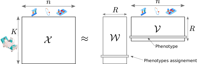
Figure 1: Illustration of the problem of patient phenotyping as a matrix factorization (specific type of tensor decomposition) without temporal dimension. A patient is a represented by a feature vector of size $n$. $\mathcal{X}$ is the input matrix of $K$ patients. The decomposition extracts both the $R$ phenotypes ($\mathcal{V}$) and the assignments of this phenotypes to patients ($\mathcal{W}$).

We now illustrate the connection between tensor decomposition and patient phenotyping, i.e. the task that consists in discovering hidden phenotypes in the data of a cohort of patients. We consider a simple case where patients are represented by a matrix $\mathcal{X}$ (second-order tensors) depicted in Figure 1: each patient is described by $n$ features. A basic decomposition of $\mathcal{X}$ is obtained as a couple of matrices ($\mathcal{V}$ of dimension $R\times n$ and $\mathcal{W}$ of dimension $K\times R$) that reconstruct the input tensors by a matrix product. The matrix $\mathcal{V}$ represents the $R$ phenotypes, i.e. linear combinations of features; and $\mathcal{W}$ is an assignment matrix. It assigns a linear combination of phenotypes to each patient.

The decomposition is obtained by minimizing the reconstruction error as follows:

$$\underset{\mathcal{W},\mathcal{V}}{\text{minimize}} ||\mathcal{X}-\mathcal{W}\mathcal{V}||_{F}^{2}$$ (1)

The minimization problem of Equation 1 is simple instance of the generic problem of tensor decomposition. It addresses the problem of patient phenotyping as one of the matrices of the decomposition is interpreted as a set of phenotypes.

It is worth noting that $R$ is a parameter of the decomposition the user has to set up. $R$ represents the assumed number of hidden phenotypes in the data. This value is typically smaller that the number of features $n$ such that the decomposition can be seen as a dimensionality reduction technique.

2.2 Tensor decomposition from temporal EHR Data

An EHR dataset has a timed event-based structure described by three dimensions: patient identifiers, care events (procedures, lab tests, drugs delivered) and time. In the previous section, a patient was described only by static features, in this section we add the temporal dimension to model the dynamics of the patients’ evolutions. We first introduce the tensor-based representation of EHR data and then, we review different techniques that address the problem of patient phenotyping from third-order tensors.

2.2.1 Tensor Based Representation of temporal EHR Data

Considering that time is discrete (e.g., events are associated to a day during the patient stay), then each patient $k\in[K]$ is represented by a matrix $\bm{X}^{(k)}$ with a 2 dimension: one dimension for time and one dimension for the type of events. Then, $x^{(k)}_{i,t}$ is a non-null value at position $(i,t)$ when, at time $t$, the patient $k$ received a care $i$. In most cases, values are categorical (boolean values 0 or 1), but sometimes they can be integer or real (e.g., a number of drugs or a measurement of a biophysiological parameter).

Additionally, if we consider that all patients have the same length, the set of patients is a three-dimensional tensor $\mathcal{X}$, i.e. a data-cube. Nevertheless, in practice, patients’ stays do not have the same duration. It ensues that each matrix $\bm{X}^{(k)}$ has its own temporal size, noted, $T_{k}$, and that the collection of matrices $\{\bm{X}^{(k)}\}_{k\in[K]}$ can not be stacked as a third-order tensor. In this case, we term this collection an irregular tensor and we use the same notation $\mathcal{X}$. We will see that some tensor decomposition approaches handle irregular tensor, but that some others require to have regular tensor (all patient’ stays share the same duration).

Figure 2 depicts an irregular tensor that represents the typical structure of the input of a patient phenotyping problem. In this figure, we assume all features are categorical, i.e. matrices are boolean valued. A black cell represents a 1 (the presence of a given event at a given time instant) and a white cell represents a 0 (absence of a given care at a given time instant).

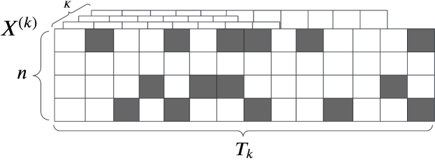
Figure 2: Illustration of an irregular tensor $\mathcal{X}=\{\bm{X}^{(k)}\}_{k\in[K]}$ representing a collection of $K$ patients stays. Each patient has its own duration $T_{k}$ but share the same set of cares (in rows). A black cell at position $(i,t)$ (i.e. $x^{(k)}_{i,t}=1$) indicates that the $i$-th care occurs at the time $t$.

2.2.2 Third-order Tensor Decomposition for Patient Phenotyping

Kiers et al. (1999) proposed PARAFAC2 which generalizes the problem described in Equation 1 to third-order irregular tensors. PARAFAC2 is formulated as follows:

$$\underset{\{\bm{U_{k}}\}_{k\in[K]},\{\bm{S_{k}}\}_{k\in[K]},\bm{V}}{\text{minimize}} \sum_{k=1}^{K}\frac{1}{2}||\bm{X_{k}}-\bm{U_{k}}\bm{S_{k}}\bm{V}||_{F}^{2}$$ (2)

subject to $$\bm{U_{k}}=\bm{Q_{k}}\bm{H},\quad\bm{Q_{k}^{T}}\bm{Q_{k}}=\bm{I},$$

where factor matrix $\bm{Q_{k}}\in\mathbb{R}^{I_{k}\times R}$ is an orthogonal matrix ($\bm{Q_{k}^{T}}\bm{Q_{k}}=\bm{I}$), and $\bm{H}\in\mathbb{R}^{R\times R}$. The constraints added to $\bm{U_{k}}$ and $\bm{Q_{k}}$ guarantee the uniqueness of the decomposition.

This uniqueness of the solution and the possibility to handle irregular tensor attract a lot of interest on the PARAFAC2 model. This formulation has been applied in a wide range of application (Fanaee-T and Gama, 2015), including the analysis of longitudinal EHRs data (Perros et al., 2019). In addition, some recent worked proposed efficient implementation to process large and sparse datasets. Perros et al. (2017) proposed SPARTan, an optimization scheme of PARAFAC2 that is a scalable and that can be parallelized, and Jang and Kang (2022) proposed DPar2 a fast and scalable PARAFAC2 decomposition for irregular dense tensors.

Nonetheless, these interesting computational properties do not ensures that the unique solution of the PARAFAC2 problem is a decomposition that identify meaningful phenotypes in practice. For instance, factor matrices can contain negative values and this does not make sense in the context of patient phenotyping. Then, alternative formulations of PARAFAC2 have been proposed to include additional constraints. Cohen and Bro (2018) proposed a non-negativity constraint on the varying mode to enhance the interpretability of the resulting factors. Roald et al. (2022) extended the constraints on all-modes. On his side, COPA (COnstrained PARAFAC2) (Afshar et al., 2018) went further by introducing various meaningful constraints in PARAFAC2 modeling: 1) the smoothness imposes latent components that change smoothly over time helps to improve the model’s interpretability and robustness; 2) the sparsity drives the solution toward phenotypes with sparse descriptions. It uses popular regularization techniques based on additional $\ell_{0}$ or $\ell_{1}$ terms; 3) the non-negativity on the decomposition.

Lastly, another practical limitation of the PARAFAC2 model is the constraint on the rank value ($R$). The decomposition techniques enforces to have $R$ lower than the dimension of all modes, including the time dimension. The number of phenotypes can not be higher than the minimum duration of an irregular third-order tensor. For care pathway analysis, this enforces that pathways shorter than $R$ have to be discarded from the dataset.

To conclude, PARAFAC2 is a very interesting model for patient phenotyping from temporal EHR data, but it imposes strong constraints on the decomposition to achieve decomposition uniqueness and the unique set of phenotypes does not necessarily make sense for clinicians. Advanced machine learning techniques have been proposed to relax some of these constraints, allowing more flexible decompositions. Thus, it allows to inject expert constraints that might lead to the extraction of more meaningful phenotypes.

2.2.3 Advanced Tensor Decomposition for Temporal Phenotyping

Using tensor decomposition became an attractive method for addressing the problem of patient phenotyping, and the development of machine learning techniques enables to develop more complex models. We identified three specific questions that have been addressed in the literature:

Dealing with additional static information

Real EHR data contain both temporal (e.g., longitudinal clinical visits) and static information (e.g., patient demographics, body mass index (BMI), smoking status, main reason for hospitalisation, etc.). It is expected that the static information impacts the temporal phenotypes, i.e. the distributions of cares deliveries along the patient visits. This problem has been addressed by TASTE (Afshar et al., 2020) and TedPar (Yin et al., 2021). TASTE takes the same input irregular tensor $\mathcal{X}$ like in PARAFAC2 and an additional matrix representing the static features of each patient. The decomposition maps input data into a set of phenotypes and a patient’s temporal evolution. Phenotypes are defined by two factor matrices: one for temporal features and one for static features.

Dealing with correlation between labtest and cares

In practice, there are strong correlation between the values of labtest measurements and cares that are given. For instance, a high concentration of glucose leads to inject insulin. The HITF model (Yin et al., 2018) allows learning the interactions between medications and diagnosis. This model has been used in CNTF (Yin et al., 2019) which proposed to model patient data as a tensor with three dimensions: lab tests, medications and time.

Supervision of tensor decomposition

Another improvement of the tensor decomposition methods is their extension to supervised decomposition. Henderson et al. (2018) proposed the PSST, Phenotyping through Semi-Supervised Tensor Factorization. It introduces a cannot-link matrix on the patient factor matrix to encourage separation in the patient subgroups. PSST resulted in phenotypes that exhibited a high degree of separation between groups of patients. Predictive Task Guided Tensor Decomposition (TaGiTeD) (Yang et al., 2017) is another framework of supervised tensor decomposition. It was thought to avoid the limitations of unsupervised existing tensor based approaches, such as the need for a large dataset to achieve meaningful results. TaGiTeD uses tensor decomposition to capture the high order event interactions, which is guided by specific prediction tasks through learning specific representations that can lead to best prediction performances. According to the authors, it achieves a good balance between interpretability and performance. Lastly, Rubik (Wang et al., 2015) and SNTF (Anderson et al., 2017) are other tensor factorization models incorporating guidance constraints to align with existing medical knowledge.

2.2.4 Temporal Dimension in Tensor Decomposition

Despite it seems very important to handle the dynamic in the evolution of a patient, most tensor decompositions do not explicitly model the temporal dependencies within the patient data. The temporal aspect is very important when it comes to constructing phenotypes of typical care profiles. The first basic decomposition models such as CP and PARAFAC2 assumes the independence of each time step, ignoring the fact that the health status of patients are highly related to their medical history. For example, in the case of dehydration of children, there are two procedures of re-hydration, one of 24 hours and the other of 48 hours. These two procedures are very similar and differ mainly in the duration and the dose of administration of a serum. CP or PARAFAC2 are unable to distinguish between both of them. the other variants of PARAFAC2 have targeted some of the latter’s vulnerabilities to fix them.

To the best of our knowledge, the temporal dependencies in the data have been handle only by the introduction of temporal regularisation terms.

COPA (Afshar et al., 2018) introduce a smoothness on patients’ pathways. According to the authors, learning temporal factors that change smoothly over time is often desirable to improve the interpretability and alleviate the over-fitting to the missing data and noise. LogPar has also introduced a smoothness regularization technique. However, both of these techniques are limited because they use only the local information to smooth the pathways without considering the temporal history to build the phenotypes. Ahn et al. (2022) proposed TATD (Time-Aware Tensor Decomposition), a tensor decomposition method that models time dependency through a smoothing regularization with Gaussian kernel.

Temporally Dependent PARAFAC2 Factorization (TedPar) (Yin et al., 2021) have been proposed to address handle long term regularization. It was designed to model the evolution of chronic diseases that progress very slowly over time. It introduces the notion of temporal transition from a phenotype to another to capture the temporal dependency. TedPar also integrated a novel idea to separate relevant and irrelevant clinical features for the progression of the target diseases. However, this method remains limiting because it uses a lot of hyperparameters that are difficult to adjust and which makes the model much more unstable.

Regarding CNTF (Yin et al., 2019), an RNN was used to take into account the ordering of the clinical events. Given the sequence $w_{1},\cdots,w_{t-1}$ describing the progression of a phenotype for a given patient, an LSTM network is used to predict $w_{t}$ than the Mean Square Error (MSE) between the real and predicted value is minimized. The idea behind this is to penalize a reconstruction model that does not allow to accurately predict the next sequence of events. It enforces to discover a decomposition that is easily predictable.

It is worth noticing that all these models do not discover temporal patterns. The temporal dimension is used to constraint the extraction of daily phenotypes by taking into account their temporal dependencies. Nonetheless, these temporal dependencies are not explicit for a physician that would like to analyze the care pathways. In the method presented in this article, we propose to extract phenotypes that describe a temporal pattern. The phenotype itself contains the information of temporal dependencies in an easily interpretable way.

2.3 Alternative Approaches for Extracting Temporal Phenotypes

If the problem of extracting temporal patterns from care pathways has not yet been addressed through tensor decomposition techniques, similar problems have been addressed by using alternative approaches. We present in this section three approaches that particularly caught our attention because it targeted similar objectives.

Temporal Extensions of Topic Models

Originally, topic modeling (or latent block models) is a statistical technique for discovering the latent semantic structures in textual document. It can estimate, at the same time, the mixture of words that is associated with each topic, and the mixture of topics that describes each document. Pivovarov et al. (2015) and Ahuja et al. (2022) proposed to consider the patients’ data as a collection of documents. Then, the topic modeling results in a set of topics representing the phenotypes. Temporal extensions of topic modeling could then be used to extract temporal phenotypes. For instance, Temporal Analysis of Motif Mixtures (TAMM) (Emonet et al., 2014) is a probabilistic graphical model designed for unsupervised discovery of recurrent temporal patterns in time series. It uses non-parametric Bayesian methods fitted using Gibbs sampling to describe both motifs and their temporal occurrences in documents. It is worth noting that the motifs have a temporal dimension. This modeling capability seems to be very interesting in patient phenotyping to derive temporal phenotypes. TAMM relies on an improved version of the Probabilistic Latent Sequential Motif (PLSM) model (Varadarajan et al., 2010), which explains how the set of all observations is supposed to be generated. VLTAMM (Variable Length Temporal Analysis of Motif Mixtures) is a generalization of TAMM that allows motifs to have different lengths and infers the length of each motif automatically. The main limitation is that they do not scale compare to optimization techniques used for tensor decomposition (Kolda and Bader, 2009). Moreover, the models are very rigid and modifying them requires deriving new samplers. These limitations prevent us from using these topic models.

Phenotypes as Embeddings

In the context of neural networks, embeddings are low-dimensional, learned continuous vector representations of discrete variables. Neural network embeddings are useful because they can reduce the dimensionality of categorical variables and meaningfully represent categories in the transformed space. The primary purposes of using embeddings are finding nearest neighbours in the embedding space and visualizing relations between categories. They can also be used as input to a machine learning model for supervised tasks. Hettige et al. (2020) introduces MedGraph, a supervised embedding framework for medical visits and diagnosis or medication codes taken from pre-defined standards in healthcare such as International Classification of Diseases (ICD). MedGraph leverages both structural and temporal information to improve the embeddings quality.

Pattern Mining Methods

Sequential pattern mining (Fournier-Viger et al., 2017) addresses the problem of discovering hidden temporal patterns. A sequential pattern would represent a phenotype by a sequence of events. The well-known problem of pattern mining, which tensor decomposition does not suffer from, is pattern deluge. This problem makes it unsuitable for practical use. Nonetheless, tensor decomposition methods are close to pattern mining approaches based on compressions. GoKrimp (Lam et al., 2014), SQS (Tatti and Vreeken, 2012) and more recently SQUISH (Bhattacharyya and Vreeken, 2017) proposed sequential pattern mining approaches that optimize an Minimum Description Length (MDL) criteria (Galbrun, 2022). Unfortunately, only GoKrimp is able to handle sequences of itemsets (i.e. with parallel events), but it extracts only sequences of items and does not allow interleaving occurrences of patterns. As representing the parallel events is a crucial aspect of phenotypes, these techniques can not answer the problem of temporal phenotyping.

3 Temporal Phenotyping: new Problem Formulation

In short, temporal phenotyping is a tensor decomposition of a third-order temporal tensor discovering phenotypes that are temporal patterns. This section formalizes the problem of temporal phenotyping that is addressed in the remaining of the article.

Let $\mathcal{X}$ be an irregular third-order tensor, also viewed as a collection of $K$ matrices of dimensions $n\times T_{k}$, where $K$ is the number of individuals (patients), $n$ is the number of features (care events), and $T_{k}$ is the duration of the observations of the $k$-th individual.

Given $R\in\mathbb{N}^{*}$, a number of phenotypes and $\omega\in\mathbb{N}^{*}$ be the duration of the phenotypes (also termed as phenotype size), temporal phenotyping aims to build:

• $\mathcal{P}\in\mathbb{R}_{+}^{R\times n\times\omega}$: a third-order tensor representing the $R$ temporal phenotypes shared among all individuals. Each temporal phenotype is a matrix of size $n\times\omega$. A phenotype represents the presence of an event at a relative time $\tau$, $0\leq\tau<\omega$. $\omega$ is the same for all phenotypes.

• $\mathcal{W}=\left\{\bm{W}^{(k)}\in\mathbb{R}_{+}^{R\times T^{\prime}_{k}}\right\}_{k\in[K]}$: a collection of $K$ assignment matrices of dimension $R\times T^{\prime}_{k}$ where $T^{\prime}_{k}=T_{k}-\omega+1$ is the size for the $k$-th individual along the temporal dimension. A non-null value at position $(r,t)$ in $\bm{W}^{(k)}$ describes the start of the phenotype $r$ at time $t$ for the $k$-th individual. A matrix $\bm{W}^{(k)}$ is also named the pathway of the $k$-th individual as it describes his/her history as a sequence of temporal phenotypes.

These phenotypes and pathways are built to accurately reconstruct the input tensor, i.e. $\mathcal{X}$. The reconstruction we propose is based on a convolution operator that takes into account the time dimension of $\mathcal{P}$ to reconstruct the input tensor from $\mathcal{P}$ and $\mathcal{W}$. The convolution operator, denoted $\circledast$, is such that $\bm{X}^{(k)}\approx\widehat{\bm{X}}^{(k)}=\mathcal{P}\circledast\bm{W}^{(k)}$ for all $k\in[K]$. Formally, this operator reconstructs each vector of the matrix $\widehat{\bm{X}^{(k)}}$ at time $t$, denoted $\widehat{\bm{x}}_{.,t}^{(k)}$, as follows:

$$\widehat{\bm{x}}_{.,t}^{(k)}=\sum_{r=1}^{R}\sum_{\tau=1}^{\min(\omega,t-1)}\bm{w}^{(k)}_{r,t-\tau}\bm{p}_{\tau}^{(r)}.$$ (3)

Intuitively, $\widehat{\bm{x}}_{.,t}^{(k)}$ is a mixture of phenotype columns that occurred at most $\omega$ time units ago, except at the beginning. At one time instant, the observed events are the sum of the $\tau$-th day of the $R$ phenotypes weighted by the $\bm{W}^{(k)}$ matrix.

Figure 3 depicts the reconstruction of one matrix $\bm{X}^{(k)}$ of an input tensor. This matrix is of length $T_{k}=14$ with $n=4$ features. Its decomposition is made of $R=3$ phenotypes of size $4\times 2$ each ($\omega=2$ and $n=4$) and a pathway of length $T^{\prime}_{k}=14-2+1=13$. A colored square in $\bm{W}^{(k)}$ indicates the start of phenotype occurrences, which can overlap in $\bm{X}^{(k)}$. For instance, the column $x^{(k)}_{.,5}$ combines the occurrence of the second day of the second phenotype (in green) and the first day of the third phenotype (in blue). Each patient is given a pathway matrix $\bm{W}^{(k)}$ based on the same phenotypes $\mathcal{P}$ and according to his input matrix $\bm{X}^{(k)}$. This means that a phenotype represents a typical pattern that might occur in the pathways of multiple patients.

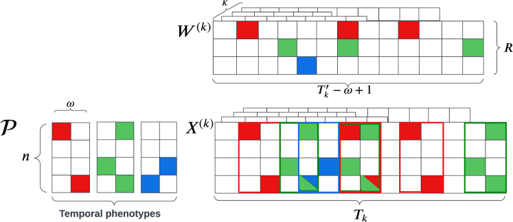
Figure 3: Illustration of a matrix reconstruction ($\bm{X}^{(k)}$) from $R=3$ phenotypes of size $\omega=2$ on the left and a care pathway ($\bm{W}^{(k)}$) on the top. Each phenotype has a specific color. Each colored cell in $\bm{W}^{(k)}$ designates the start of a phenotype occurrence in the reconstruction (surrounded with a colored rectangle in $\bm{X}^{(k)}$). A cell with two colors received the contribution of two occurrences of different phenotypes.

Then, the problem of temporal phenotyping consists in discovering both the $\mathcal{P}$ and $\mathcal{W}$ tensors such that it reconstructs well the input tensor.

4 SWoTTeD Model

SWoTTeD is a tensor decomposition model for temporal phenotyping. The generic problem of temporal phenotyping presented above is complemented by some additional hypothesis to guide the solving toward practically interesting solutions. These hypothesis are implemented through the definition of a reconstruction loss and regularization terms. This section presents the detail of the SWoTTeD model.

4.1 Temporal Phenotyping as a Minimization Problem

As in the case of the classical tensor decomposition problem, temporal phenotyping is a problem of minimizing the error between the input tensor and its reconstruction. Equation 3 details the reconstruction of a patient matrix.

SWoTTeD considers the decomposition of binary tensors, i.e. $\mathcal{X}\in\{0,1\}$. It corresponds to data that describe the absence/presence of events. In this case, we assume the input tensor $\mathcal{X}$ follows a Bernoulli distribution and we use the loss function for binary data proposed by Hong et al. (2020). The resulting reconstruction loss, $\mathcal{L}^{\circledast}$, is defined as follows:

$$\mathcal{L}^{\circledast}(\hat{\mathcal{X}},\mathcal{X})=\sum_{k=1}^{K}\sum_{t=1}^{T_{k}}\sum_{i=1}^{n}log(\hat{x}^{(k)}_{i,t}+1)-x^{(k)}_{i,t}log(\hat{x}^{(k)}_{i,t})$$ (4)

This reconstruction loss is super-scripted by $\circledast$ to remind that it is based on the convolution operator described in Equation 3.

SWoTTeD also includes two regularization terms: sparsity and non-succession regularization. Sparsity regularization on $\mathcal{P}$ aims to enforce feature selection and improve the interpretability of phenotypes. It is implemented through an $L_{1}$ term. We chose this popular regularization technique among several others, as it has shown its practical effectiveness.

We also propose a phenotype non-succession regularization to prevent undesirable decomposition, as illustrated in Figure 4. The described situation is a successive occurrence of the same event. This situation is often encountered in care pathways as a treatment might be a care delivery over several days. In this case, there are two opposite alternatives to decompose the matrix with equal reconstruction errors ($\mathcal{L}^{\circledast}$): the first alternative (at the top) is to describe the treatment as a daily care delivery and to assume that a patient received the same treatment three days in a row; the second alternative (at the bottom) is to describe the treatment as a succession of three care deliveries, but that is received only once. SWoTTeD implements the second solution as one of our objective is to unveil temporal patterns, i.e. phenotypes that correlate temporally some events.

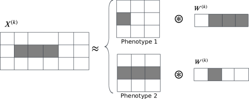
Figure 4: Example of alternative decompositions of a sequence of similar events with the same $\mathcal{L}^{\circledast}$ value. Phenotype 1 does not capture the sequence of events, whereas phenotype 2 does. The information is reported in the pathway in the case of phenotype 1.

To guide the decomposition toward our preferred one, we add a term to penalize a reconstruction that uses the same phenotype on successive days. If a phenotype occurs one day, reoccurring within the next $\omega$ days will cost. Formally, the non-succession regularization is defined as follows and depends only on the patient pathway $\bm{W^{(k)}}$:

$$\mathcal{S}(\bm{W}^{(k)})=\sum_{r=1}^{R}\sum_{t=1}^{T^{\prime}_{k}}\max\left(0,w^{(k)}_{r,t}\log\left(\sum_{\tau=t-\omega}^{t+\omega}w^{(k)}_{r,\tau}\right)\right).$$ (5)

This equation can be seen as a weighted logged convolution. The weight is $w_{r,t}$. Intuitively, the more present is the phenotype, the more expensive a new occurrence within the same time window will be. The inner $\log$ term sums all possible undesirable occurrences of the same phenotype $r$ at time $t$. The $\log$ function is used to attenuate the effect of this term and to have a null value when $w^{(k)}_{r,t}=1$ surrounded with $0$ (the ideal case, depicted in the second decomposition of Figure 4). Despite the apparent complexity of this term, it can be efficiently computed with vectorization techniques.

The final loss function of SWoTTeD is given by the weighted sum of the reconstruction error, the sparsity and the non-succession regularization:

$$\ell=\mathcal{L}^{\circledast}\left(\mathcal{P}\circledast\mathcal{W},\mathcal{X}\right)+\alpha\,\,||\mathcal{P}||_{1}+\beta\,\sum_{k=1}^{K}\mathcal{S}\left(\bm{W}^{(k)}\right)$$ (6)

where $\alpha$ and $\beta$ are two positive real-valued hyperparameters. Note that the two regularization terms have opposite effects: the sparsity prefers phenotypes with a lot of zeros, while the non-succession prefers to use non-null values in phenotypes than in pathways. A choice of hyper-parameters may impact the quality of the discovered phenotypes.

4.2 Optimization Framework

The problem of discovering temporal phenotypes turns out to minimize the overall loss function $\ell$ as follows:

$$\underset{\{\bm{W}^{(k)}\},\mathcal{P}}{\arg\min} \mathcal{L}^{\circledast}\left(\mathcal{P}\circledast\mathcal{W},\mathcal{X}\right)+\alpha\,\,||\mathcal{P}||_{1}+\beta\,\sum_{k=1}^{K}\mathcal{S}\left(\bm{W}^{(k)}\right)$$ (7)

subject to $$\forall k,\,0\leq\bm{W}^{(k)}\leq 1,\quad 0\leq\mathcal{P}\leq 1.$$

The minimization problem presented in Equation 7 restricts the values’ range to $[0,1]$ in order to interpret $\mathcal{P}$ (resp. $\mathcal{W}$) as the probability of having an event (resp. a phenotype) at a given time. These constraints are sound with our assumption of a Bernoulli distribution. Another motivation to normalize pathway is related to the non-succession regularization, $\mathcal{S}(\bm{W}^{(k)})$. As mentioned earlier, this regularization term is null when there are isolated ones in the pathway. If values are higher than 1, the non-succession regularization penalizes each presence of a phenotype even if isolated. This behavior is not expected.

To optimize the overall loss function $\ell$ (see Equation 6), we use an alternating minimization strategy and projected gradient descent (PGD). Alternating Least Square (ALS) algorithm optimizes one variable individually, using a gradient descent step, with all other variables fixed. Alternating the process of minimization guarantees reduction of the cost function, until convergence. PGD handles the non-negativity and the normalization constraints. It works by clipping the values after each iteration.

Data: $\{\bm{X^{(k)}}|k\in[K]\}$: patient stays, $R$: the number of temporal phenotypes, $\omega$: the size of the temporal window, $\alpha$, $\beta$: loss hyper-parameters.

Result: $\mathcal{P}$: phenotype tensor, $\{\bm{W^{(k)}}|k\in[K]\}$: phenotype occurrences in patient stays

$\mathcal{P}\leftarrow\mathcal{U}(0,1)$

$\mathcal{W}\leftarrow\mathcal{U}(0,1)$

for each epoch do

       for each mini-batch $\mathcal{B}$ do

             Update $\mathcal{P}$ by descending its gradient

             $\mathcal{P}\leftarrow clip(\mathcal{P},0,1)$

            

            for $k\in\mathcal{B}$ do

                   Update $\bm{W}^{(k)}$ by descending its gradient

                   $\bm{W}^{(k)}\leftarrow clip(\bm{W}^{(k)},0,1)$

                  

             end for

            

       end for

      

end for

(notation: $clip(x,0,1)=min(max(x,0),1)$)

Algorithm 1 Optimization Framework for SWoTTeD

(notation: $clip(x,0,1)=min(max(x,0),1)$)

The optimization framework of SWoTTeD is illustrated in Algorithm 1. In each mini-batch, we first sample a collection of patient matrices ${\{\bm{X}^{(k)}|k\in\mathcal{B}\}}$ with $\mathcal{B}$ being the patient’s indices of a batch. The phenotype tensor $\mathcal{P}$ is firstly optimized given ${\{\bm{W}^{(k)}|k\in\mathcal{B}\}}$ values, then ${\{\bm{W}^{(k)}|k\in\mathcal{B}\}}$ is optimized given $\mathcal{P}$ values.

Out of the classical optimization parameters such as the learning rate, the batch size, and the number of epochs, the main hyper-parameters of SWoTTeD are $R$, the number of temporal phenotypes, $\omega$, the temporal size of phenotypes and $\alpha$, $\beta$ the loss hyper-parameters. Compared to the recent deep neural network architecture, the number of hyperparameters of SWoTTeD is limited and they are interpretable.

4.3 Applying SWoTTeD on Test Sets

The tensor decomposition presented in the previous section corresponds to the training of SWoTTeD. This model is made up of temporal phenotypes, $\mathcal{P}$. In the minimization problem presented in Equation 7, the assignment tensor $\mathcal{W}$ contains a set of free parameters that are to be discovered during the learning procedure but are not kept in the model because they are specific to the train set.

Despite tensor decomposition being an unsupervised classification task, the results of the decomposition can be evaluated on a test set. The objective is to assess whether the unveiled phenotypes are useful for decomposing new care pathways. In this case, we can conclude that they capture meaningful phenotypes.

Applying a tensor decomposition on a test dataset, $\mathcal{X}^{\prime}$, consists in finding the optimal assignment given a fixed set of temporal phenotypes. $\mathcal{X}^{\prime}$ is a third-order tensor with $K^{\prime}$ individuals, each having their duration, but sharing the same $n$ features defined in the training dataset. The optimal assignment is obtained by solving the following optimization problem that is similar to Equation 7, but with a fixed $\widehat{\mathcal{P}}$ (the optimal phenotypes obtained from the decomposition of a train set).

$$\underset{\mathcal{W}^{\prime}}{\arg\min} \mathcal{L}^{\circledast}\left(\widehat{\mathcal{P}}\circledast\mathcal{W}^{\prime},\mathcal{X}^{\prime}\right)+\beta\,\sum_{k=1}^{K}\mathcal{S}\left(\bm{W}^{\prime(k)}\right)$$ (8)

subject to $$0\leq\mathcal{W}\leq 1.$$

This optimization problem can be solved by a classical gradient descent algorithm. Similarly to the training, we use PGD for the normalization constraint.

4.4 Algorithms Complexity

SWoTTeD is based on an optimization procedure for training the model or applying it on a test dataset. This section provides an estimation of the time complexity involved in computing the loss $\ell$ (see Equation 7). Subsequently, the complexity of the entire learning procedure can be approximated by multiplying this complexity with the number of epochs.

Let $\mathcal{X}$ be a dataset with $K$ patients, $n$ medical features, and a maximum hospital stay length of $\bar{T}$; let $R$ be the desired number of phenotypes described over a temporal window of size $\omega$. The complexity to compute the reconstruction $\mathcal{P}\circledast\mathbf{W}^{(k)}$ is given by:

$$O\left(K\times\bar{T}\times R\times n\times\omega\right)$$

It follows that the complexity to compute the error $\mathcal{L}^{\circledast}$ (see Equation 4) is as follows:

$$O\left(\left(R\times\omega+1\right)\times K\times\bar{T}\times n\right)$$

The complexity of an epoch of SWoTTeD (see Equation 7) includes the complexity of the regularization terms, as outlined below:

• The complexity of the $L_{1}$ norm is $O\left(n\times\omega\times R\right)$ (i.e., the size of $\mathcal{P}$).

• The complexity of the non-succession regularization term $\mathcal{S}(\mathbf{W}^{(k)})$ is $O\left(K\times R\times\bar{T}\times\omega\right)$.

In comparison to non-temporal tensor decomposition techniques (e.g., CNTF), the complexity of SWoTTeD considers the $\omega$ factor that corresponds to the temporal width of phenotypes. While SWoTTeD is more expressive, it requires more computing resources than CNTF. On the other hand, the reconstruction and non-succession term are based on convolution operators that benefit from material optimization. Thus, we anticipate that the efficiency of the optimization process will be preserved.

5 Experimental Setup

SWoTTeD is implemented using the PyTorch framework (Paszke et al., 2019), along with PyTorch Lightning for easy integration into other deep learning architectures. The model is available in the following repository: https://gitlab.inria.fr/hsebia/swotted. In the experiments, we used two equivalent implementations of SWoTTeD: a classical version handle irregular tensor and a fast-version handle only regular tensor benefiting from improved vectorial optimization. Additionally, we provide the deposit which includes all the materials needed to reproduce the experiments except for the use case: https://gitlab.inria.fr/tguyet/swotted_experiments. All experiments have been conducted with desktop computers, without the use of GPU acceleration.

We trained the model with an Adam optimizer to update both tensors $\mathcal{P}$ and $\mathcal{W}$. The learning rate is set to $10^{-3}$ with a batch size of $50$ patients. We fine-tuned the hyperparameters $\alpha$ and $\beta$ by testing different values and selecting the ones that yielded the best reconstruction measures (see experiments in Section 6.1). The tensors $\mathcal{P}$ and $\mathcal{W}$ are initialized randomly using a uniform distribution ($\mathcal{U}(0,1)$).

The quality measures reported in the results have been computed on test sets. For each experiment, 70% of the dataset is used for training, and 30% is used for testing. The test set patients are drawn uniformly.

5.1 Datasets

In this section, we present the open-access datasets used for quantitative evaluations of SWoTTeD, including comparisons with competitors. We conducted experiments on both synthetic and real-world datasets to evaluate the reconstruction accuracy of SWoTTeD against its competitors. Synthetic datasets are used to quantitatively assess the quality of the hidden patterns as they are known in this specific case.

5.1.1 Synthetic Data

The generation of synthetic data involves the reverse process of the decomposition. Generating a dataset follows three steps:

1. A third-order tensor of phenotypes $\mathcal{P}$ is generated by randomly selecting a subset of medical events for each instant of the temporal window of each phenotype.

2. The patient pathways $\mathcal{W}$ are generated by randomly selecting the days of occurrence for each phenotype along the patient’s stay, ensuring that the same phenotype cannot occur on successive days. Bernoulli distributions with $p=0.3$ are used for this purpose.

3. The patient matrices of $\mathcal{X}$ are then computed using the reconstruction formulation proposed in Equation 3.

However, this reconstruction can result in values greater than $1$ when multiple occurrences of phenotypes sharing the same drug or procedure deliveries accumulate. To fit our hypothesis of binary tensors, we binarize the tensor resulting from the process above by projecting non-null values to $1$.

The default characteristics of the synthetic datasets subsequently generated for various experiments are as follows: $K=500$ patients, $n=20$ care events, $R=4$ phenotypes of length $\omega=3$, and stays of $T_{k}=10$ days for all $k$.

5.1.2 Real-world Datasets

The experiments conducted on synthetic datasets are complemented by experiments on three real-world datasets, which are publicly accessible. We selected one classical dataset in the field of patient phenotyping (namely the MIMIC database) and two sequential datasets coming from very different contexts. Table 1 summaries the main characteristics of these datasets.

• MIMIC dataset: MIMIC-IV is a large-scale, open-source and disidentified database providing critical care data for over $40,000$ patients admitted to intensive care units at the Beth Israel Deaconess Medical Center (BIDMC) (Johnson et al., 2020). We used the version 0.4 of MIMIC-IV. The dataset has been created from the database by selecting a collection of patients and gathering their medical events during their stay. For the sake of reproducibility, the constitution of the dataset is detailed in supplementary materials. In addition, the code used to generate our final datasets is provided in the deposit of experiments.

• E-Shop dataset: This UCI dataset contains information on clickstream from online store offering clothing for pregnant women. Data are from five months of 2008 and include, among others, product category, location of the photo on the page, country origin of the IP address and product price in US dollars.

• Bike dataset: This contains sequences of locations where shared bikes where parked in a city. Each item represents a bike sharing station and each sequence indicate the different locations of a bike over time. The specificity of this dataset is to contain only one location per date.

For each of these datasets, we also created a “regular” version, which contains individuals’ pathways sharing the same length. This dataset is utilized with our fast-SWoTTeD implementation that benefit from better code-vectorization. The creation of these datasets involves two steps: 1) selecting individuals with pathway durations greater than or equal to $T$, and 2) truncating the end of the pathways if they exceed $T$ in length. The selection of the values for $T$ is a balance between maintaining the maximum length and retaining the maximum number of individuals.

Table 1: Real-world dataset characteristics: $n$ number of features, $K$ number of individuals, $\bar{T}$ mean duration

Dataset	$n$	$K$	$\bar{T}$
MIMIC-IV	$2,717$	$200$	$9.62\pm 12.7$
MIMIC-IV-reg	$825$	$200$	$10$
Bike	$21,078$	$67$	$11.43\pm 5.93$
Bike-reg	$5,243$	$67$	$10$
E-Shop	$24,026$	$317$	$13.79\pm 11.19$
E-Shop-reg	$5,212$	$317$	$10$

We remind that our case study presents another datasets of patients staying in the Greater Paris University Hospitals for qualitative analysis of phenotypes. This dataset will be detailed in Section 7.

5.2 Competitors

We compare the performance of SWoTTeD against four state-of-the-art phenotyping models. These models were selected based on the following criteria: 1) their motivation to analyze EHR datasets, 2) their competitiveness in terms of accuracy compared to other approaches, 3) the availability of their implementations, and 4) their handling of temporality.

We remind that SWoTTeD is the only tensor decomposition technique able to extract temporal patterns. Our competitors extract daily phenotypes.

The four competing models are the followings:

• CNTF (Yin et al., 2019), a tensor decomposition model factorizing tensors with varying temporal size, assuming the input tensor to follow a Poisson distribution, but it has shown its effectiveness on binary data; CNTF is our primary competitor since it incorporates temporal regularization, aiming to capture data dynamics.

• PARAFAC2 (Kiers et al., 1999), original decomposition model with non-negative constraint. This decomposition is based on Frobenius norm. We use the Tensorly implementation (Kossaifi et al., 2016).

• LogPar (Yin et al., 2020), a logistic PARAFAC2 for learning low-rank decomposition with temporal smoothness regularization. We choose to include LogPar in the competitors’ list because, like SWoTTeD, it is designed for binary tensors and assumes a Bernoulli distribution. LogPar can handle only regular tensors.

• SWIFT (Afshar et al., 2021), a tensor decomposition model minimizing the Wasserstein distance between the input tensor and its reconstruction. SWIFT does not assume any explicit distribution, thus it can model complicated and unknown distributions.

For each experiment, we manually configure their hyper-parameters to ensure the fairest possible comparisons.

5.3 Evaluation Metrics

In tensor decomposition, a primary objective is to reconstruct accurately an input tensor. We adopt the $FIT\in(-\infty,1]$ (Bro et al., 1999) to measure the quality of a model’s reconstruction:

$$FIT_{X}=1-\frac{\sum_{k=1}^{K}||\bm{X}^{(k)}-\bm{\widehat{X}}^{(k)}||_{F}}{\sum_{k=1}^{K}||\bm{X}^{(k)}||_{F}}$$ (9)

where the input tensor $\mathcal{X}$ serves as the ground truth, the resulting tensor is denoted $\mathcal{\widehat{X}}$ and $||\cdot||_{F}$ is the Frobenius norm. The higher the value of $FIT$, the better. The $FIT$ measure is also used to compare phenotypes and patient pathways when hidden patterns are known a priori,i.e., for synthetic datasets. Thus, $FIT_{P}$ (resp. $FIT_{W}$) denotes the reconstruction quality of $\mathcal{P}$ (resp. $\mathcal{W}$).

It is worth noting that $FIT_{X}$ measure is computed on a test set except for SWIFT and PARAFAC2. Evaluation on test sets requires the model to be able to project a test set on existing phenotypes (see Section 4.3), but SWIFT and PARAFAC2 do not have this capability.

We also introduce a similarity measure between two sets of phenotypes to evaluate empirically the uniqueness of solutions and a diversity measure of a set of phenotypes, adapted from similarity measures introduces by Yin et al. (2019).

Let $\mathcal{P}=\{\bm{P}_{1},\dots,\bm{P}_{R}\}$ and $\mathcal{P}^{\prime}=\{\bm{P}^{\prime}_{1},\dots,\bm{P}^{\prime}_{R}\}$ be two sets of phenotypes defined over a temporal window size $\omega$. The principle of our similarity measure is to find the optimal matching between the phenotypes of the two sets, and to compute the mean of the (dis)similarities between the matching pairs of phenotypes. More formally, in the case of Cosine similarity, we compute:

$$sim(\mathcal{P},\mathcal{P}^{\prime})=\max_{\pi}\frac{2}{(R)(R-1)}\sum_{(i,j)\in\pi}\cos(\bm{P}_{i},\bm{P}^{\prime}_{j})$$

where $\pi$ denotes an isomorphism between $\mathcal{P}$ and $\mathcal{P}^{\prime}$, and $\cos(\cdot,\cdot)$ is a cosine distance between two temporal phenotypes. It is computed as the mean of the cosine similarity between each time slice of the phenotype:

$$\cos(\bm{P},\bm{P}^{\prime})=\frac{1}{\omega}\sum_{i=1}^{\omega}\frac{\bm{p}_{:,i}.\bm{p}^{\prime}_{:,j}}{||\bm{p}_{:,i}||\times||\bm{p}_{:,j}||}$$

In practice, we first compute a matrix of costs and use the Hungarian algorithm to find the optimal matching ($\pi$). Finally, we compute the measure with $\pi$.

The diversity measure of the set of phenotypes aims to quantify the redundancy among the phenotypes. In this case, we expect to have low similarities between the phenotype.

Let $\mathcal{P}=\{\bm{P}_{1},\dots,\bm{P}_{R}\}$ be a set of $R$ phenotypes defined over a temporal window of size $\omega$, the cosine diversity is defined by:

$$div(\mathcal{P})=\frac{2}{(R)(R-1)}\sum_{1\leq i<j\leq R}1-\cos(\bm{P}_{i},\bm{P}_{j}).$$

6 Experiments and Results

In this section, we present the experiments we conducted to evaluate SWoTTeD. The main questions we investigate are the following:

• What is the effect of the loss hyper-parameters on the reconstruction accuracy? For that, we investigate in Section 6.1 the influence of parameters $\alpha$, the weight of sparsity term; $\beta$, the weight of the non-succession term; and the influence of the normalization. In addition, we designed an experiment to demonstrate the effectiveness of the non-succession term. One of the main objectives of these data-intensive experiments is to identify a setting for the hyper-parameters that provides good results on average.

• Does SWoTTeD compete with state-of-the-art algorithms? To address this question, the section 6.2 presents the comparison of SWoTTeD with selected competitors (see Section 5.2) in terms of both reconstruction quality and computing time. As the other tensor decomposition methods do not extract temporal phenotypes, we evaluate SWoTTeD with different values of $\omega$, including $\omega=1$ for more fairness.

• Is SWoTTeD robust to data-noise? This question is of a particular interest when dealing with EHR datasets. EHR datasets can contain many meaningless events, some important events of a care pathway may not be reported in the databases. The Section 6.3 presents experiments conducted on synthetic datasets to assess the robustness of SWoTTeD against additive and destructive noise.

• Are the outputs of SWoTTeD stable? The stability of the method denotes its capability to extract the same phenotypes during different similar runs. This property is expected for SWoTTeD to be trustworthy by users. In the experiment presented in Section 6.4, we evaluate the similarity between the sets of phenotypes extracted in different runs and the diversity of each set of phenotypes.

6.1 SWoTTeD Loss Hyper-Parameters

This section focuses on the loss hyper-parameters of SWoTTeD. The objective of these experiments is to provide a comprehensive review of the effect of the loss parameters and to assess whether the model behaves as expected. We start by presenting some experiments on synthetic datasets and then confirm the results on the three real-world datasets.

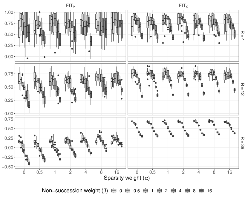
Figure 5: $FIT_{P}$ (left) and $FIT_{X}$ (right) of SWoTTeD with $\omega=3$ on synthetic data. Each graph represents a box plot for 10 runs.

In this first experiment, we generated synthetic datasets using $R$ hidden phenotypes ($R=4,12$ or $36$) with a window size $\omega=3$. SWoTTeD is run 10 times with different parameters values:

• $\alpha=\{0,0.5,1,2,4,8,16\}$ representing the weight of the sparsity term in the loss

• $\beta=\{0,0.5,1,2,4,8,16\}$ representing the weight of the phenotype non-succession term in the loss

We collected the $FIT_{X}$ and $FIT_{P}$ metric values on a test set. The first metric assesses the quality of the reconstruction, while the second assesses whether the discovered phenotypes match the expected ones.

Figure 5 depicts the $FIT$ measures with respect to the parameters $\alpha$ and $\beta$ (with normalization activated). One general result is that the $FIT_{X}$ values are high. Values exceeding 0.5 indicate significantly good reconstructions, and those surpassing 0.8 imply that the differences between two matrices become imperceptible. Furthermore, we observe that a good $FIT_{P}$ implies a good $FIT_{X}$. This illustrates that in tensor decomposition, an accurate discovery of hidden phenotypes is beneficial for achieving a high-quality tensor reconstruction. However, as we see with $R=32$, a good $FIT_{X}$ does not necessarily mean that the method discovered the correct phenotypes.

A second general observation is that the same evolution of the FIT with respect to $\beta$ is observed in most of the settings: the $FIT$ increases between $\beta=0$ and $\beta=1$ and then it decreases quickly for higher values. This demonstrates two key points: 1) the inclusion of non-succession terms improves the reconstruction accuracy, and 2) on average, a value of $0.5$ yields the best results. Regarding the parameter $\alpha$, we notice a slight improvement in $FIT$ measures as $\alpha$ increases. This is more evident with $R=36$, and when we focus on results with $\beta=0.5$, we observed that $\alpha=1$ is, on average, the best compromise for the sparsity term.

One last observation is that as $R$ increases, $FIT$ measures decrease. This may be counter-intuitive, as the expected results is that the $FIT_{X}$ decreases with increasing $R$ (as we will discuss with real-world dataset results later on). In this experiment, $R$ corresponds to both the rank of the decomposition and the number of hidden phenotypes we used to generate the dataset. As $R$ increases, the dataset contains more variability and denser events, making the reconstruction task challenging and leading to a slightly decrease of the $FIT$ measure. $FIT_{X}$ maintains a high value even with $R=36$ but $FIT_{P}$ has low values in this case. We explain this observation by colinearities between phenotypes.

Finally, we complemented our analysis of parameters by specifically investigating the non-succession term introduced in SWoTTeD. To assess its efficiency, we generated synthetic datasets with $4$ random phenotypes and $6$ phenotypes that have been designed to contain successions of similar events (see Figure 4).

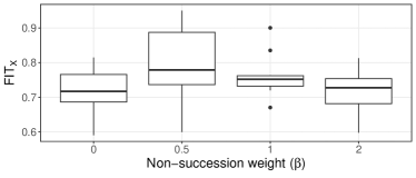
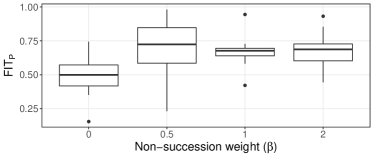
Figure 6: Comparison of $FIT_{X}$ (left) and $FIT_{P}$ (right) with respect to $\beta$ hyper-parameter on a synthetic dataset with hidden phenotypes having repeated successive events.

Figure 6 depicts the $FIT_{X}$ and $FIT_{p}$ values with respect to $\beta$ ($\alpha$ is set to $2$ in this experiment). We observe clearly that $FIT_{P}$ are higher when $\beta$ is not null, i.e. when we use the non-succession term in SWoTTeD ($FIT_{P}=0.75$ instead of $0.50$ when $\beta=0$). The best median $FIT_{X}$ is close to $0.8$ and occurs when $\beta=0.5$. This confirms that adding the non-succession regularization disambiguates the situation illustrated in Figure 4 and helps the model to correctly reconstruct the latent variables. We conclude that the use of the non-succession regularization increases the decomposition quality, whether there are event repetitions in phenotypes or not (see Figure 5).

6.2 SWoTTeD against Competitors

In this section, we compare SWoTTeD against competitors based on the ability to achieve accurate reconstructions, to extract hidden phenotype effectively and to efficiently handle large scale datasets. To address these various dimensions, we use both synthetic and real-world datasets.

For the real-world datasets, we use truncated versions because LogPar requires regular tensors. Additionally, we remind that $FIT$ values are evaluated on test sets, except for SWIFT and PARAFAC2, for which we utilize the error on the training set since these approaches can not be applied on test sets.

6.2.1 SWoTTeD Accuracy on Daily Phenotypes

This experiment compares the accuracy of SWoTTeD against competitors on 20 synthetic datasets. For the sake of fairness, the datasets are generated with daily hidden phenotypes ($\omega=1$). Our goal is to evaluate the accuracy of phenotypes extracted by SWoTTeD compared to the ones of state-of-the-art models.

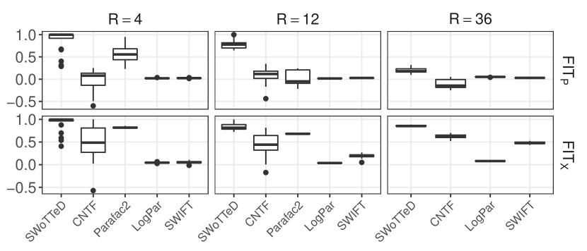
Figure 7: $FIT_{P}$ values (at the top) and $FIT_{X}$ values (at the bottom) of SWoTTeD vs competitors on synthetic data with $\omega=1$.

Figure 8: Critical difference diagrams between SWoTTeD and its competitors (based on $FIT_{X}$ metric on the left, and on $FIT_{P}$ metric on the right). The lower the rank, the better. Horizontal bars indicate statistical non-significant difference between models. The significancy is obtained with a Wilcoxon signed-rank test ($\alpha=0.05$).

The results, depicted in Figure 7, show that SWoTTeD achieves the best performance in terms of $FIT_{X}$ and $FIT_{P}$ metrics. The second-best model is PARAFAC2. It achieves good tensor reconstructions but it fails to identify the hidden phenotypes (low $FIT_{P}$ values). The analysis of the phenotypes show that PARAFAC creates mixtures of phenotypes. Note that PARAFAC2 has no value for $R=36$ because $R$ must be lower than the maximum of every dimension.

The reconstructions of CNTF are also satisfying but the phenotypes are different from the expected one. Our intuition is that assuming Poisson distribution is not effective for these data following a Bernoulli distribution. The two other competitors are assumed to be adapted to these data but in practice, we observe that they have reconstructed the tensors with lower accuracy, and the extracted phenotypes are less similar to the hidden ones compare to SWoTTeD.

To confirm these results, Figure 8 depicts critical difference diagrams. It ranks the methods based on the Wilcoxon signed-rank test on $FIT_{X}$ or $FIT_{P}$ metrics. The diagram shows that SWoTTeD is ranked first, and the difference in $FIT_{P}$ compared to other methods is statistically significant.

The high-quality performance of SWoTTeD can be attributed to two main factors. Firstly, SWoTTeD offers greater flexibility in reconstructing input data by allowing the overlap of different phenotypes and their arrival with a time lag. Secondly, SWoTTeD employs a loss function that assumes a Bernoulli distribution, which fits better binary data.

6.2.2 SWoTTeD against Competitors on Real-world Datasets

In this section, we evaluate SWoTTeD against its competitors on the three real-world datasets to confirm that previous results applies on real-world data. We vary $R$ from $4$ to $36$, and $\omega$ from $1$ to $5$ for SWoTTeD, and we compare $FIT_{X}$ values. It is worth noting that $FIT_{P}$ can not be evaluated in this case as hidden phenotypes are unknown. Each setting is ran 10 times with different train and test sets.

Figure 9: Reconstruction error $FIT_{X}$ of SWoTTeD ($\omega=1,3,5$) and its competitors on real-world datasets and for different values of $R$.

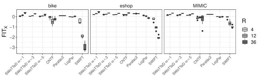
Figure 15: Reconstruction error $FIT_{X}$ of SWoTTeD ($\omega=1,3,5$) and its competitor on real-world datasets and for different values of $R$.

Figure 9 summarizes the results. Across all datasets, SWoTTeD achieves an average $FIT_{X}$ of $0.21$. PARAFAC2 achieves the second best reconstructions but remind that $FIT_{X}$ is evaluated on the train set. CNTF has good results except for the bike dataset. Specifically, SWoTTeD outperforms all the competitors with comparable $R$ on bike and MIMIC datasets regardless of the phenotype size. On the eshop dataset, CNTF exhibits good performances with $R=36$ and outperforms SWoTTeD when $\omega>1$. Nonetheless, SWoTTeD with $\omega=3$ becomes better than CNTF. LogPar and SWIFT have the worse $FIT_{X}$ on average. For sake of graphic clarity, SWIFT is not represented in this Figure. Their $FIT_{X}$ values are below $-0.5$. The complete Figure is provided in Appendix (see Figure 15, page 15).

The figure presents results for three different values of $R$. As expected, $FIT_{X}$ of SWoTTeD increases with $R$. Intuitively, real-world datasets contain a diversity and a large number of hidden profiles. With more phenotypes, the model becomes more flexible and can capture the diversity in the data more effectively, resulting in more accurate tensor reconstructions.

We also observe that while $FIT_{X}$ decreases slightly as the phenotype size ($\omega$) increases, all values remains higher than those of CNTF, except for bike with $R=36$. This suggests that SWoTTeD with $\omega>1$ discovers phenotypes that are both complex and accurate. It may seem counterintuitive that the $FIT$ does not decrease. In fact, the number of models’ parameters as we increase the size of the phenotype. However, these parameters are not completely free. Larger phenotypes also add more constraints to the reconstruction due to temporal relations, which can introduce errors when a phenotype is only partially identified. The more complex is the phenotype, the more likely there is a slight difference between the mean description and its instances.

The most important result of this experiment is that the reconstruction with temporal phenotypes competes with the reconstruction with daily phenotypes. This means that SWoTTeD strikes a balance between a good reconstruction of the input data and an extraction of rich phenotypes. Furthermore, the temporal phenotypes – with $\omega$ strictly higher than $1$ – convey a rich information to users by describing complex temporal arrangements of events.

6.2.3 Time Efficiency

Figure 10 illustrates the computing times of the training process on real-world datasets. It compares the computing time of SWoTTeD with its competitors under different setting (varying values of $R$ and $\omega$). We have excluded SWIFT from this Figure as its computing time is several orders of magnitude slower than the other competitors due to the computation of Wasserstein distances.

This figure shows that our implementation of SWoTTeD is one order of magnitude faster than CNTF or LogPar. This efficiency is achieved thanks to an efficient vectorized implementation of the model. The mean computing times on a standard desktop computer for SWoTTeD are $70.42s\pm 18.37$, and $102.83s\pm 209.34$ and $14.34s\pm 1.03$ for the datasets Bike, Eshop, and MIMIC, respectively.

Regarding the parameters of SWoTTeD, we observe that the computing time grows linearly with the number of phenotypes. More surprisingly, the size of the phenotypes has only a minor impact on computing time. This can be attributed to the efficient implementation of convolutions in the PyTorch framework.

Figure 10: Computing time (log-scale) of SWoTTeD and its competitors.

Despite the relatively high theoretical complexity of the reconstruction procedure, this experiment demonstrates that SWoTTeD has low computing times and can scale to handle large datasets.

6.3 SWoTTeD Robustness to Data Noise

Noisy data are a common challenge encountered in the analysis of medical data. Physicians may make errors during data collection. Some exams may not be recorded in electronic health records and the data collection instruments themselves may be unreliable, resulting in inaccuracies within datasets. These inaccuracies are commonly referred to as noise. Noise can introduce complications as machine learning algorithms may interpret it as a valid pattern and attempt to generalize from it. Therefore, we conducted an assessment of the robustness of our model against simulated noisy data.

We considered two types of common noise that are due to data entry errors: 1) the additive noise due to occurrences of additional events in patient’s hospital stays, and 2) the destructive noise, due to important events that have not been copied. We start by generating 20 synthetic datasets that are divided into training and test sets. Only the training set is disturbed, and the $FIT$ value is measured over the test set. The idea behind disturbing only the training set is to assess SWoTTeD’s ability to capture meaningful phenotypes in the presence of noise that can be generalized over a non-disturbed test set. For additive noise, we inject additional events positioned randomly into the $\mathcal{X}$ tensor. The number of added events per patient is determined according to a Poisson distribution with a parameter $\lambda$. We vary $\lambda$ from $2$ to $25$. The noise level is normalized by the number of ones in the dataset (i.e. the number of events). For instance, $0.3$ means that $30\%$ of additional events have been injected into the data. Values greater than $1.0$ for noise addition indicates than more than half of the events are random. For the destructive noise, we iterate over all the events of all the patients in $\mathcal{X}$, and delete them based on a Bernoulli distribution with a parameter $p$. We vary $p$ from $0$ to $0.7$.

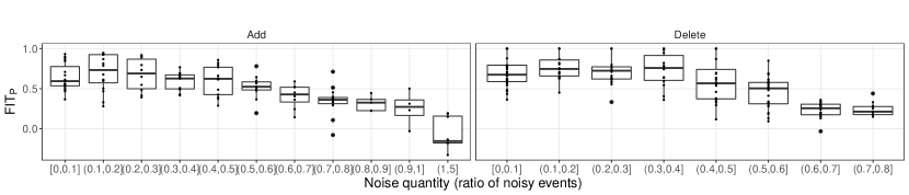
Figure 11: $FIT_{P}$ values of SWoTTeD on synthetic data as a function of normalized noise (% of new or deleted events).

Our focus was primarily on SWoTTeD’s ability to derive correct phenotypes from noisy data, as measured by the $FIT_{P}$ metric.

Figure 11 displays the values of $FIT_{P}$ obtained with various noise ratios. In the case of added events, we notice that $FIT_{P}$ decreases as the average number of added events per patient increases. However, the quality of reconstruction remains above zero even when the average number of added events per patient reaches 10. In the case of deleting events, we notice that $FIT_{P}$ starts to decrease when the ratio of missing events exceeds $0.3$. In an extreme case where we have 70% of missing events, SWoTTeD still manages to have a positive phenotype reconstruction quality.

Consequently, we can conclude that our model exhibits robustness to noisy data, particularly in the case of missing data. Being robust to additive noise is inherent to the tensor decomposition technique used to uncover hidden patterns in the data. This experiment further confirms the interest of tensor decomposition when data are noisy. Interestingly, adding some random noise even resulted in improved accuracy. We explain this by the relatively low number of epochs (200): some randomness in the data fasten the convergence of optimization algorithms. With fewer epochs, the model discovered better phenotypes in the presence of noise. Being robust to destructive noise is more promising. In real-world dataset, especially in care pathways that is our primary application, missing events might be numerous. The results show that our model can discover the hidden phenotypes with high accuracy even with a lot of (random) missing events.

6.4 Uniqueness of and Diversity in SWoTTeD Results

Solving tensor decomposition problems with an ALS optimization algorithm does not guarantee a convergence toward a global minimum or even a stationary point, but only to a solution where the objective function stops decreasing (Kolda and Bader, 2009). The final solution can also be highly dependent on the initialization and of the training set. Similarly, SWoTTeD does not come with convergence guarantees, but we can empirically evaluate the diversity of solutions obtained across different runs.

The experiments conducted on synthetic datasets illustrated that different runs of SWoTTeD converges toward the expected phenotypes (as detailed in Section 6.1). However, it can not conclusively determine the uniqueness of solutions, as it heavily relies on the random phenotypes that have been generated. we exclusively employ real-world datasets in this section.

Figure 12: Cosine dissimilarity between pairs of sets of phenotypes with respect to the phenotypes’ size for SWoTTeD, and CNTF. The lower the dissimilarity, the more similar are the sets of phenotypes between each run.

In this experiment, we delve into the sets of phenotypes in our real-world datasets. For each dataset, we run SWoTTeD 10 times and compare the sets of phenotypes using average cosine dissimilarity.

Figure 12 depicts the cosine dissimilarity obtained with $R=4$, $12$ and $36$ for SWoTTeD (with varying phenotype sizes) and CNTF. Lower dissimilarity values indicate greater similarity between phenotypes from one run to another, which is preferable.

With $R=36$, the cosine dissimilarity is below $0.5$ for all datasets. In the case of SWoTTeD, it generally exceeds $0.3$. This observation suggests that there may be multiple local optima, where the optimization procedure must make choices among the phenotypes to represent. Consequently, the convergence location may depend on the initial state. The dissimilarity values show both high and low values, that correspond to have “clusters” of similar solutions.

On average, CNTF exhibits slightly better than SWoTTeD, but the difference with SWoTTeD (${\omega=1}$) is not significant across the dataset.

For $\omega=3$ or $5$, we observe higher dissimilarity between the runs. Part of this increase can be explained by the metric used: cosine similarity tends to be higher for high-dimensional vectors (i.e. larger phenotype sizes). This is because small differences in one dimension can lead to a significant decrease in cosine similarity, and the probability of such differences increases with the number of dimensions.

We conducted a qualitative analysis of the differences between the sets of phenotypes and found them to be almost the same. However, we observed some discrepancies with a few extra or missing events. These events are recurrent in the data, but not necessarily related to a pathway. As the number of phenotypes is limited, it is better to include such events in a phenotype to improve reconstruction accuracy. Their weak association with other events can lead to variations between runs.

Figure 13: Cosine dissimilarity between pairs of phenotypes with respect to the phenotypes’ size for SWoTTeD, and CNTF. The higher the dissimilarity, the more diverse.

Continuing our investigation of the similarities between phenotypes, we also evaluate the diversity of phenotypes within the sets of $R$ phenotypes. We computed the pairwise cosine dissimilarity between phenotypes within each set extracted by the different runs of SWoTTeD. The objective is to evaluate each method’s ability to extract a diverse set of phenotypes. It is worth noting that this orthogonality constraint, proposed by Kolda (2001) for instance, is not directly coded in SWoTTeD (nor in CNTF). The diversity is expected as a side-effect of the reconstruction loss with a small set of phenotypes. For datasets with numerous latent behaviors, a diverse set of phenotypes ensures a better coverage of the data.

Figure 13 presents the distributions of cosine dissimilarity values. In this experiment, higher cosine dissimilarity values indicate greater diversity, which is desirable. We can first notice the results are correlated to the analysis of uniqueness. Diverse sets of phenotypes corresponds to robust settings. This may be explained by the fact that the diverse sets extracted the complete set.

To summarize this section, we conclude that SWoTTeD consistently converges toward sets of looks alike phenotypes on the real-world datasets for different runs. These sets contain diverse phenotypes, highlighting the SWoTTeD’s ability to discover non-redundant latent behaviors in temporal data. Despite these promising results, we recommend running SWoTTeD multiple times on new datasets to enhance the confidence in the results.

7 Case Study

The experiments demonstrated that SWoTTeD is able to accurately and robustly identify hidden phenotypes in synthetic data and to accurately reconstruct real-world data. In this section, we illustrate that the extracted temporal phenotypes are meaningful. For this purpose, we used SWoTTeD on an EHR dataset from the Greater Paris University Hospitals and showed the outputted phenotype to clinicians for interpretation.

The objective of this case study is to describe typical pathways of patients that have been admitted into intensive care units (ICU) during the first waves of COVID-19 in the Greater Paris region, France. The typical pathways are representative of treatment protocols that have actually been implemented. Describing them may help hospitals to gain insight into their management of treatments during a crisis. In the context of COVID-19, we know that the most critical cases are patients with comorbidities (diabetes, hypertension, etc.). This complicates the analysis of these patients’ care pathways because they blend multiple independent treatments. In such a situation, cutting edge tools for pathway analysis are helpful to disentangle the different treatments that have been delivered.

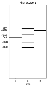
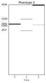
Figure 14: Five phenotypes discovered for the 4th epidemic wave. Each gray cell represents the presence of a drug (in rows) at a relative time instant (in columns). The darker the cell, the higher the value. Cell values lie in the range $[0,1]$.

Care pathways of COVID-19 patients have been obtained from the data warehouse of the Greater Paris University Hospitals. We create one dataset per epidemic wave of COVID-19 for the first four waves. The periods of these waves are those officially defined by the French government. The patients selected for this study are adults (over 18 years old) with at least a positive PCR. For each patient, we create a binary matrix that represents the patient’s care events (drugs deliveries and procedures) during the first $10$ days of his/her stay in the Intensive Care Unit (ICU). Epidemiologists selected $85$ types of care events ($58$ types of drugs and $27$ types of procedures) based on their frequency and relevance for COVID-19. Drugs are coded using the third level of ATC codes and procedures are coded using the third level of CCAM codes.

In the following, we present the results obtained for the fourth wave (from 2021-07-05 to 2021-09-06) which holds $2,593$ patients and $21,325$ care events. We run SWoTTeD to extract $R=8$ phenotypes of length $\omega=3$. We run $1,000$ epochs with a learning rate of $10^{-3}$.

Figure 14 illustrates five of the eight phenotypes extracted from the fourth wave. At first glance, we can see that these phenotypes are sparse. This makes them almost easy to interpret: a phenotype is an arrangement of at most 7 care events, all with high weights. In addition, they make use of the time dimension: each phenotype describes the presence of care events on at least two different time instants. Thus, it demonstrates that the time dimension of a phenotype is meaningful in the decomposition. These phenotypes have been shown to a clinician for interpretation. It was confirmed that they reveal two relevant care combinations: some combinations of cares sketch the disease background of patients (hypertension, liver failure, etc.) while others are representative of treatment protocols. The phenotype 1 has been interpreted as a typical protocol for COVID-19. Indeed, L04A code referring to Tocilizumab has become a standard drug to help patients with acute respiratory problems avoid mechanical ventilation. In this phenotype, clinicians detect a switch from the prophylactic delivery of Tocilizumab (the first day) to a mechanical ventilation identified through the use of typical sedative drugs (L04A: Lidocaine, J01X: Metronidazole and N05C: Midazolam). This switch, including the discontinuation of Tocilizumab treatment, is a typical protocol. Nevertheless, further investigations are required to explain the presence of antibiotics (J01D: Prednisone and H02A: Cefotaxime). Phenotype 5 illustrates a severe septic shock: a patient in this situation will be monitored (DEQ), injected with dopamine (EQL) to induce cardiac activity, and with insulin (A10A) to manage the patient’s glycaemia. This protocol is commonly encountered in ICU, and is applied for COVID-19 patients in critical condition.

The previously detailed phenotypes illustrate that SWoTTeD disentangles generic ICU protocols and specific treatments for COVID-19. Other phenotypes have also been readily identified by clinicians as corresponding to treatments of patients having specific medical backgrounds. The details can be found in supplementary materials. Their overall conclusion is that SWoTTeD extracts relevant phenotypes that uncover some real practices.

8 Conclusion and Perspectives

The state-of-the-art tensor decomposition methods are limited to the extraction of phenotypes that only describe a combination of correlated features occurring the same day. In this article, we proposed a new tensor decomposition task that extracts of temporal phenotypes, i.e., phenotypes that describe a temporal arrangement of events. We also propose SWoTTeD, a tensor decomposition method dedicated to the extraction of temporal phenotypes.

SWoTTeD has been intensively tested on synthetic and real-world datasets. The results show that it outperforms the current state-of-the-art tensor decomposition techniques on synthetic data by achieving the best reconstruction accuracies of both the input data and the hidden phenotypes. The results on synthetic data show that the reconstruction accuracy compete with the state-of-the art, but extract information through the temporal phenotypes that is not captured by other approaches.

In addition, we proposed a case study on COVID-19 patients to demonstrate the effectiveness of SWoTTeD to extract meaningful phenotypes. This experiment illustrates the relevance of the temporal dimension to describe typical care protocols.

The results of SWoTTeD are very promising and open new research lines in machine learning, temporal phenotyping and care pathway analytics. For future work, we plan to extend SWoTTeD to extract temporal phenotypes described over variable size windows. It would also be interesting to make the reconstruction more flexible for alternative applications. In particular, our temporal phenotypes are rigid sequential patterns: they describe the strict succession of days. This was expected to describe treatments in ICU, but some other applications might expect two consecutive days of a phenotype to match two days that are not strictly consecutive (with a gap in between). This is an interesting but challenging modification of the reconstruction which can be computationally expensive.

Appendix A Details about Experiments

A.1 Synthetic Dataset

The code to generate synthetic data is available in the “gen_data.py” file. We also provide a jupyter notebook “run_SWoTTeD_synthetic_data.ipynb” that allows the reader to run readily SWoTTeD on a synthetic dataset.

A.2 MIMIC-IV Dataset

The database can be accessed via this link https://mimic.mit.edu/. Once the database is set up in a Postgres database, the Jupyter notebook “CohortConstruction.ipynb” can be run to prepare the dataset: it builds the cohort of patients and the input tensors used in the experiments. We also provide a notebook “run_SWoTTeD_mimic.ipynb” to guide the reader to execute SWoTTeD on MIMIC-IV.

The availability of this data preparation enables anyone to create the exact dataset we used for our experiments and to compare his/her own results with ours.

Appendix B Additional results

B.1 Impact of normalization

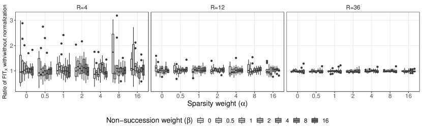
Figure 16: Ratio of the $FIT_{X}$ metric with and without normalization of SWoTTeD on synthetic datasets. A ratio above $1$ indicates a benefit of using normalization on the reconstruction accuracy.

Similar experiments were conducted without normalization. The Figure 16 depicts the ratio of $FIT_{X}$ with and without normalization. We observe that the values are very close to 1. On average, normalization appears to increase the $FIT$ measure (ratio above 1), but it is not significant. We conclude from this experiment that normalization does not clearly improves the reconstruction accuracy neither the quality of the extracted phenotypes. Therefore, we recommend keeping the normalization constraint because it guarantees to limit $\mathcal{W}$’s values are limited to the range $[0,1]$ and they can be interpreted as probabilities.

B.2 Comparison FIT computed on train or test datasets

The objective of this experiment is to show that the phenotypes discovered does not overfit the train dataset. To demonstrate this, we computed the $FIT_{X}$ values computed on test and train sets.

Figure 17 presents the results obtained for our four real-world datasets. We observe that the $FIT_{X}$ computed on train and test datasets are on average similar both for SWoTTeD and CNTF. It shows that neither SWoTTeD nor CNTF overfits the train dataset. This result contributes to show that the extracted phenotypes are meaningful.

Figure 17: $FIT_{X}$ metric computed on test and train datasets for realworld datasets.

B.3 Comparison of Time Efficiency of SWoTTeD vs FastSWoTTeD

We remind that FastSWoTTeD is an implementation of SWoTTeD for datasets having all sequences with the same length. In this case, it is possible to increase the computational efficiency of the implementation with vectorization techniques. We also remind that we did not used GPU to accelerate the training.

In this experiment we generated 200 synthetic sequences with all same lengths ($T=20$) and $40$ features. We run the two models on the same datasets and we measure the training time, and the $FIT_{X}$ on a test set.

The Figure 18 depicts the computing times with respect to the number of hidden phenotypes ($R$). The boxplot averages the result for different model settings. We clearly see that FastSWoTTeD is more than one order of magnitude faster than SWoTTeD.

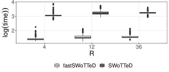
Figure 18: $\log(time)$ (en seconds) for training SWoTTeD and FastSWoTTeD models.

Figure 19: $FIT_{X}$ on synthetic datasets obtained with SWoTTeD and FastSWoTTeD models.

The Figure 19 depicts the $FIT_{X}$ obtained with the two implementations of SWoTTeD. We observe that the two implements have achieves the same $FIT_{X}$. The difference can be explained by the randomness in the training process, combined with small floating point errors that propagate differences between the decompositions. Statistically, the differences are not significant between these two models.

Appendix C Case Study Details

C.1 Dataset preparation

In our case study, we used data from the Greater Paris University Hospitals. For the sake of health data security and privacy, these data have been pseudo-anonymized and it is not possible to export them out of the hospital infrastructure. Then, all experiments on the AP-HP dataset were conducted on hospital servers through secured access.

In addition, all the experiments have been approved by the Ethical committee of AP-HP which is in charge to inform patients about their data usage for research purposes, to obtain their informed consent and to validate the appropriateness of data access by researchers.

In accordance with epidemiologists, we created one dataset per epidemic wave of COVID-19 for the first four waves. The periods of these waves are those officially defined by the French government:

• wave 1: 2020-03-01 - 2020-07-06, $8,561patients$, $81,517$ care events

• wave 2: 2020-07-07 - 2021-01-04, $10,444$ patients, $91,824$ care events

• wave 3: 2021-01-05 - 2021-07-05, $14,667$ patients, $139,045$ care events

• wave 4: 2021-07-05 - 2021-09-06, $2,593$ patients, $21,325$ care events

The patients selected for this study are:

• adults (over 18 years old)

• at least a positive PCR test to witness the COVID-19 status of the patient

• admitted in an Intensive Care Unit (ICU). ICU includes here the historical and de novo units. The latter have been by set up to respond urgently to the massive arrival of patients.

For each patient we create a binary matrix that represents its care pathway.

We collected medical procedures and drugs delivered during the 10 first days in an Intensive Care Unit (ICU). All care pathways start from the entrance in an ICU. This means that all cares received at hospital before the entrance in ICU are ignored. If a patient is admitted several times in an ICU, each visit is independent of the others.

We take at most 10 days of the visits, and stays shorten than 2 days are discarded. A 10 days period is assumed to be long enough to be representative of a patient treatment in ICU. 40% of the patients have a length of stay lower than 10 days.

Drugs are coded using ATC codes and procedures are coded using CCAM codes. CCAM is the French Common Classification of medical procedures. Each code is a type of medical event in the input tensor. The date of occurrence of an event is determined by the number of days before the beginning of mechanical ventilation. More specifically, it means that the sampling rate is one day. In the data warehouse, procedure and drug deliveries are timestamped but, according to clinicians, these timestamps are not reliable (for instance, care deliveries are entered in the system at once at the end of the day). If the length of stay is lower than 10 days (whatever the discharge reason), then the temporal dimension of its matrix is its length of stay. More specifically, all matrices do not have the same temporal dimensions.

We first selected the 500 most frequent drugs and the 200 most frequent procedures over a very large space. Then, Drugs have been clustered at the 3rd ATC level, and procedures at the 3th level of CCAM coding hierarchy. Indeed, different drug names may correspond to the same kind of cares. Thus, we group drugs using the coding hierarchy of the ATC and of the CCAM. A second manual selection has been done by physicians to keep only the most relevant features in the context of COVID-19. In the end, $85$ types of care events ($58$ types of drugs and $27$ types of procedures) have been selected by physicians based on their frequency and relevance for COVID-19.

It is worth noticing that we do not have access to a reliable information about the duration of a drug prescription. For instance, we noticed that antibiotic drugs are delivered to patients on a single day each time, but not several days in a row. Nonetheless, clinicians indicates that antibiotic are always delivered for several days to be effective. This is a limitation to identifier temporal phenotypes, but we prefer to not pre-processed the data to prevent from having too questionable results.

The following table presents the parameters used for the results presented in Section C.2.

Parameter	Value
$R$	$8$/$20$
$\omega$	$3$/$5$
$\alpha$	$0.5$
$\beta$	$0.5$
$\lambda$	$10^{-3}$
epochs	$1,000$
batch size	$64$

C.2 Additional Results on Case Study

In this section, we present the results obtained for the four first waves of the COVID-19 pandemic. We start by providing results about the reconstruction accuracy for several settings of SWoTTeD. Then, we illustrate the reconstruction of some patient matrices. Finally, we present the graphical and detailed descriptions of the phenotypes obtained with $R=8$ phenotypes and $\omega=3$.

Note that these results need additional investigations by clinicians to provide reliable interpretations. For this reason, we do not provide more detailed interpretations of phenotypes in this document.

C.2.1 Reconstruction Accuracy

Table 2 gives the $FIT_{X}$ values obtained on the four AP-HP datasets (four first waves of the pandemic). The values are close to the ones obtained on the MIMIC-IV dataset. These values are positive, indicating that the reconstruction is reasonably good on average.

Table 2: Reconstruction accuracy measured by $FIT_{X}$ of the AP-HP datasets (one per wave) with different settings of SWoTTeD. Bold values are the bests.

Wave	$R=8$	$R=20$	$R=20$
	$\omega=3$	$\omega=3$	$\omega=5$
w1	0.17	0.27	0.22
w2	0.15	0.25	0.23
w3	0.15	0.23	0.23
w4	0.15	0.25	0.27

We can notice that SWoTTeD achieves better reconstruction with $R=20$ than with $R=8$. Indeed, with more phenotypes, the decomposition becomes easier. The drawback of having more phenotypes is to discover simpler patterns, i.e. involving fewer events.

Finally, increasing the size of the temporal phenotypes does not improve the reconstruction. Larger temporal phenotypes means a more constrained reconstruction.

C.2.2 Reconstructions

Figure 20: Examples of patient matrix reconstruction (with $R=8$ and $\omega=3$). For each patient, the original matrix is on the left, the reconstructed matrix is on the right.

Figure 20 illustrates the reconstructions of two patient’s matrices. The patients are in the dataset of the fourth wave, and the reconstruction use $R=8$ and $\omega=3$.

These reconstructions illustrate the behaviour we observed: 1) a reconstruction contains all the events of the input matrix, 2) some additional events appear in the reconstruction. For the patient on the left ($id:596$), the reconstruction contains, with significant weights, the five care events of the initial matrix. But, an additional event appears in the reconstruction (with a low weight). For the patient on the right ($id:1992$), the first day of the reconstruction contains a lot of lightly weighted events, but it reconstructs well the complex combination at time $6$.

A possible explanation of this behaviour can be found in the weak quality of the data. As we notice, there may miss some events. The additional events in the reconstruction may witness such misinformed care deliveries. This hypothesis remains to be investigated.

C.2.3 Phenotypes of the First Wave

Figure 22 illustrates the phenotypes that have been extracted. These phenotypes are detailed in the following tables.

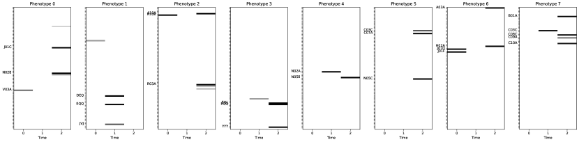
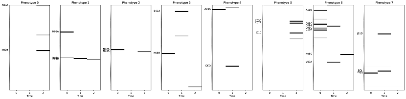
Figure 21: Graphical representation of the phenotypes of the first wave.

Figure 22: Graphical representation of the phenotypes of the second wave.

Phenotype 1
Event code	Description	Time
C02C	Urapidil, hypertension	0.00	0.00	0.17
J01C	Amoxicilline	0.00	0.00	1.00
N02B	Paracetamol	0.00	0.00	1.00
N03A	Pregabaline	0.00	0.00	0.33
V03A	Oxygen	0.61	0.00	0.00

Phenotype 2
Event code	Description	Time
C09C	Irbesartan, ARB	0.39	0.00	0.00
DEQ	Electrocardiogram	0.00	1.00	0.00
EQQ	Cardiac monitoring	0.00	1.00	0.00
JVJ	Dialysis	0.00	0.66	0.00

Phenotype 3
Event code	Description	Time
A10A	Insuline	0.00	0.00	1.00
A10B	Metformine	1.00	0.00	0.00
R03A	Adrenergics, inhalants	0.00	0.00	1.00
R03B	Drugs for obstructive airway diseases	0.00	0.00	0.39
R06A	Antihistamines	0.00	0.00	0.28

Phenotype 4
Event code	Description	Time
ENL	Monitoring of intra-arterial pressure	0.00	0.38	0.00
EQL	Dopamine	0.00	0.00	1.00
EQQ	Cardiac monitoring	0.00	0.00	1.00
YYY	Rescucitation procedures	0.00	0.00	1.00

Phenotype 5
Event code	Description	Time
N02A	Morphines	0.00	1.00	0.00
N05B	Hydroxizine, sedation	0.00	0.00	1.00

Phenotype 6
Event code	Description	Time
C03C	Furosemide	0.00	0.00	0.73
C07A	Bisoprolol	0.00	0.00	1.00
N05C	Midazolam, sedation	0.00	0.00	1.00

Phenotype 7
Event code	Description	Time
A03A	Phloroglucinol	0.00	0.00	0.88
H02A	Prednisone, antibiotic	0.00	0.00	1.00
J01D	Cefotaxime	1.00	0.00	0.00
J01F	Azithromicine	1.00	0.00	0.00

Phenotype 8
Event code	Description	Time
B01A	Antithrombotic agents	0.00	0.00	1.00
C03C	Furosemide	0.00	1.00	0.00
C08C	Amlodipine	0.00	0.00	1.00
C09A	Ramipril	0.00	0.00	0.54
C10A	Statine	0.00	0.00	0.89

C.2.4 Phenotypes of the Second Wave

Figure 22 illustrates the phenotypes that have been extracted. These phenotypes are detailed in the following tables.

Phenotype 1
Event code	Description	Time
A03A	Phloroglucinol	0.00	0.00	0.42
J01E	Sulfonamides and trimethoprim	0.00	0.00	0.24
N02B	Paracetamol	0.00	0.00	1.00

Phenotype 2
Event code	Description	Time
H02A	Prednisone, antibiotic	1.00	0.00	0.00
P02C	Ivermectine	0.26	0.00	0.00
R03A	Adrenergics, inhalants	0.00	1.00	0.00
R03B	Drugs for obstructive airway diseases	0.00	0.00	0.50

Phenotype 3
Event code	Description	Time
N02A	Morphines	1.00	0.00	0.00
N03A	Pregabaline	0.00	0.00	0.63

Phenotype 4
Event code	Description	Time
B01A	Antithrombotic agents	0.00	1.00	0.00
J01F	Azithromicine	0.00	0.22	0.00
N05B	Hydroxizine, sedation	1.00	0.00	0.00
JVJ	Dialysis	0.00	0.00	0.38

Phenotype 5
Event code	Description	Time
A06A	Constipation	0.00	0.35	0.00
A10A	Insuline	1.00	0.00	0.00
DEQ	Electrocardiogram	0.00	1.00	0.00

Phenotype 6
Event code	Description	Time
C03C	Furosemide	0.00	0.00	1.00
C07A	Bisoprolol	0.00	0.00	1.00
J01C	Amoxicilline	0.00	0.00	1.00
J01X	Metronidazole	0.00	0.00	0.27

Phenotype 7
Event code	Description	Time
A03A	Phloroglucinol	0.00	0.19	0.00
A10B	Metformine	0.80	0.00	0.00
C03A	Hydrochlorothiazide	0.14	0.00	0.00
C08C	Amlodipine	1.00	0.00	0.00
C09A	Ramipril	0.00	0.80	0.00
C09C	Irbesartan, ARB	0.52	0.00	0.00
C10A	Statine	1.00	0.00	0.00
J01M	Ciprofloxacine	0.16	0.00	0.00
N05C	Midazolam, sedation	0.00	0.00	1.00
V03A	Oxygen	0.00	0.70	0.00

Phenotype 8
Event code	Description	Time
J01D	Cefotaxime	0.00	1.00	0.00
DEQ	Electrocardiogram	0.00	0.01	0.00
EQL	Dopamine	0.00	1.00	0.00
EQQ	Cardiac monitoring	1.00	0.00	0.00

C.2.5 Phenotypes of the Third Wave

Figure 24 illustrates the phenotypes that have been extracted. These phenotypes are detailed in the following tables.

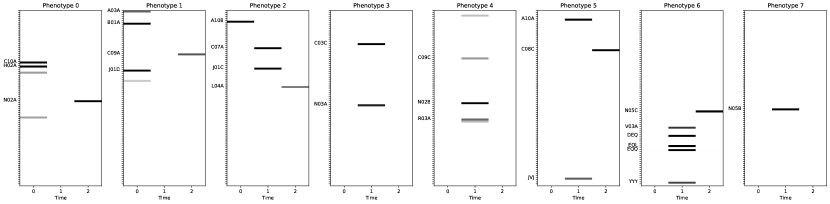
Figure 23: Graphical representation of the phenotypes of the third wave.

Figure 24: Graphical representation of the phenotypes of the fourth wave.

Phenotype 1
Event code	Description	Time
C10A	Statine	1.00	0.00	0.00
H02A	Prednisone, antibiotic	1.00	0.00	0.00
J01E	Sulfonamides and trimethoprim	0.38	0.00	0.00
N02A	Morphines	0.00	0.00	1.00
P02C	Ivermectine	0.37	0.00	0.00

Phenotype 2
Event code	Description	Time
A03A	Phloroglucinol	0.61	0.00	0.00
B01A	Antithrombotic agents	1.00	0.00	0.00
C09A	Ramipril	0.00	0.00	0.66
J01D	Cefotaxime	1.00	0.00	0.00
J01X	Metronidazole	0.21	0.00	0.00

Phenotype 3
Event code	Description	Time
A10B	Metformine	1.00	0.00	0.00
C07A	Bisoprolol	0.00	1.00	0.00
J01C	Amoxicilline	0.00	1.00	0.00
L04A	Tocilizumab	0.00	0.00	0.51

Phenotype 4
Event code	Description	Time
C03C	Furosemide	0.00	1.00	0.00
N03A	Pregabaline	0.00	0.88	0.00

Phenotype 5
Event code	Description	Time
A06A	Constipation	0.00	0.26	0.00
C09C	Irbesartan, ARB	0.00	0.40	0.00
N02B	Paracetamol	0.00	1.00	0.00
R03A	Adrenergics, inhalants	0.00	0.60	0.00
R03B	Drugs for obstructive airway diseases	0.00	0.27	0.00

Phenotype 6
Event code	Description	Time
A10A	Insuline	0.00	1.00	0.00
C08C	Amlodipine	0.00	0.00	1.00
JVJ	Dialysis	0.00	0.63	0.00

Phenotype 7
Event code	Description	Time
N05C	Midazolam, sedation	0.00	0.00	1.00
V03A	Oxygen	0.00	0.79	0.00
DEQ	Electrocardiogram	0.00	1.00	0.00
EQL	Dopamine	0.00	1.00	0.00
EQQ	Cardiac monitoring	0.01	1.00	0.01
YYY	Rescucitation procedures	0.00	0.74	0.00

Phenotype 8
Event code	Description	Time
N05B	Hydroxizine, sedation	0.00	1.00	0.00

C.2.6 Phenotypes of the Fourth Wave

Figure 24 illustrates the phenotypes that have been extracted. These phenotypes are detailed in the following tables.

Phenotype 1
Event code	Description	Time
B01A	Antithrombotic agents	0.00	0.00	1.00
J01E	Sulfonamides and trimethoprim	0.00	0.00	0.33
R03A	Adrenergics, inhalants	0.00	0.00	0.53
R03B	Drugs for obstructive airway diseases	0.00	0.00	0.26
R06A	Antihistamines	0.23	0.00	0.00

Phenotype 2
Event code	Description	Time
H02A	Prednisone, antibiotic	0.00	1.00	0.00
J01D	Cefotaxime	0.00	0.00	1.00
J01X	Metronidazole	0.00	0.40	0.00
L04A	Tocilizumab	0.59	0.00	0.00
N01B	Lidocaine	0.00	0.21	0.00
N05C	Midazolam, sedation	0.00	1.00	0.00

Phenotype 3
Event code	Description	Time
A10B	Metformine	0.00	0.00	1.00
N03A	Pregabaline	0.00	0.00	1.00
P02C	Ivermectine	0.00	0.00	0.45
EQQ	Cardiac monitoring	0.00	1.00	0.00

Phenotype 4
Event code	Description	Time
A03A	Phloroglucinol	0.00	0.00	1.00
C03D	Spironolactone, cardiac failure	0.00	0.28	0.00
C09C	Irbesartan, ARB	0.94	0.00	0.00
C09D	Anti-hypertensor ARB	0.00	0.00	0.16
J01F	Azithromicine	0.00	0.24	0.00

Phenotype 5
Event code	Description	Time
C03C	Furosemide	0.00	1.00	0.00
N02A	Morphines	0.00	0.00	1.00
JVJ	Dialysis	0.00	0.49	0.00

Phenotype 6
Event code	Description	Time
A10A	Insuline	1.00	0.00	0.00
J01C	Amoxicilline	0.00	0.00	1.00
DEQ	Electrocardiogram	1.00	0.00	0.00
EQL	Dopamine	0.50	0.00	0.00

Phenotype 7
Event code	Description	Time
C08C	Amlodipine	0.00	0.00	1.00
N02B	Paracetamol	0.00	0.00	1.00
N05B	Hydroxizine, sedation	0.00	0.00	1.00

Phenotype 8
Event code	Description	Time
A06A	Constipation	0.00	0.27	0.00
C01B	Amiodarone, cardiac failure	0.00	0.29	0.00
C07A	Bisoprolol	0.00	1.00	0.00
C09A	Ramipril	0.81	0.00	0.00
C10A	Statine	0.00	0.00	1.00
J01M	Ciprofloxacine	0.00	0.18	0.00
V03A	Oxygen	0.00	0.00	0.58

References

- Perros et al. [2017] Ioakeim Perros, Evangelos E Papalexakis, Fei Wang, Richard Vuduc, Elizabeth Searles, Michael Thompson, and Jimeng Sun. SPARTan: Scalable PARAFAC2 for large and sparse data. In Proceedings of the International Conference on Knowledge Discovery and Data Mining (SIGKDD), pages 375–384, 2017.
- Fanaee-T and Gama [2016] Hadi Fanaee-T and João Gama. Tensor-based anomaly detection: An interdisciplinary survey. Knowledge-Based Systems, 98:130–147, 2016.
- Anandkumar et al. [2014] Animashree Anandkumar, Rong Ge, Daniel Hsu, Sham M Kakade, and Matus Telgarsky. Tensor decompositions for learning latent variable models. Journal of machine learning research, 15:2773–2832, 2014.
- Becker et al. [2023] Florian Becker, Age K. Smilde, and Evrim Acar. Unsupervised EHR-based phenotyping via matrix and tensor decompositions. WIREs Data Mining and Knowledge Discovery, page e1494, 2023.
- Yin et al. [2019] Kejing Yin, Dong Qian, William K. Cheung, Benjamin C. M. Fung, and Jonathan Poon. Learning phenotypes and dynamic patient representations via RNN regularized collective non-negative tensor factorization. In Proceedings of the AAAI Conference on Artificial Intelligence, pages 1246–1253, 2019.
- Kolda and Bader [2009] Tamara G Kolda and Brett W Bader. Tensor decompositions and applications. SIAM review, 51(3):455–500, 2009.
- Zachariah et al. [2012] Dave Zachariah, Martin Sundin, Magnus Jansson, and Saikat Chatterjee. Alternating least-squares for low-rank matrix reconstruction. IEEE Signal Processing Letters, 19(4):231–234, 2012.
- Kiers et al. [1999] Henk AL Kiers, Jos MF Ten Berge, and Rasmus Bro. PARAFAC2–part I. A direct fitting algorithm for the PARAFAC2 model. Journal of Chemometrics: A Journal of the Chemometrics Society, 13(3-4):275–294, 1999.
- Fanaee-T and Gama [2015] Hadi Fanaee-T and Joao Gama. Eigenevent: an algorithm for event detection from complex data streams in syndromic surveillance. Intelligent Data Analysis, 19(3):597–616, 2015.
- Perros et al. [2019] Ioakeim Perros, Evangelos E. Papalexakis, Richard Vuduc, Elizabeth Searles, and Jimeng Sun. Temporal phenotyping of medically complex children via PARAFAC2 tensor factorization. Journal of Biomedical Informatics, 93:103125, 2019.
- Jang and Kang [2022] Jun-Gi Jang and U Kang. Dpar2: Fast and scalable PARAFAC2 decomposition for irregular dense tensors. In Proceedings of the International Conference on Data Engineering (ICDE), pages 2454–2467, 2022.
- Cohen and Bro [2018] Jeremy E Cohen and Rasmus Bro. Nonnegative PARAFAC2: A flexible coupling approach. In International Conference on Latent Variable Analysis and Signal Separation, pages 89–98. Springer, 2018.
- Roald et al. [2022] Marie Roald, Carla Schenker, Vince D Calhoun, Tülay Adali, Rasmus Bro, Jeremy E Cohen, and Evrim Acar. An AO-ADMM approach to constraining PARAFAC2 on all modes. SIAM Journal on Mathematics of Data Science, 4(3):1191–1222, 2022.
- Afshar et al. [2018] Ardavan Afshar, Ioakeim Perros, Evangelos E. Papalexakis, Elizabeth Searles, Joyce Ho, and Jimeng Sun. COPA: Constrained PARAFAC2 for sparse and large datasets. In Proceedings of the International Conference on Information and Knowledge Management (CIKM), pages 793–802, 2018.
- Afshar et al. [2020] Ardavan Afshar, Ioakeim Perros, Haesun Park, Christopher R. deFilippi, Xiaowei Yan, Walter F. Stewart, Joyce Ho, and Jimeng Sun. TASTE: temporal and static tensor factorization for phenotyping electronic health records. In Proceedings of the Conference on Health, Inference, and Learning (CHIL), pages 193–203, 2020.
- Yin et al. [2021] Kejing Yin, William K Cheung, Benjamin CM Fung, and Jonathan Poon. TedPar: Temporally dependent PARAFAC2 factorization for phenotype-based disease progression modeling. In Proceedings of the SIAM International Conference on Data Mining (SDM), pages 594–602, 2021.
- Yin et al. [2018] Kejing Yin, William K Cheung, Yang Liu, Benjamin CM Fung, and Jonathan Poon. Joint learning of phenotypes and diagnosis-medication correspondence via hidden interaction tensor factorization. In Proceedings of the International Joint Conference on Artificial Intelligence (IJCAI), pages 3627–3633, 2018.
- Henderson et al. [2018] Jette Henderson, Huan He, Bradley A Malin, Joshua C Denny, Abel N Kho, Joydeep Ghosh, and Joyce C Ho. Phenotyping through semi-supervised tensor factorization (PSST). In Proceedings of the Annual Symposium of AMIA, pages 564–573, 2018.
- Yang et al. [2017] Kai Yang, Xiang Li, Haifeng Liu, Jing Mei, Guotong Xie, Junfeng Zhao, Bing Xie, and Fei Wang. TaGiTeD: Predictive task guided tensor decomposition for representation learning from electronic health records. In Proceedings of the AAAI Conference on Artificial Intelligence, pages 2824–2830, 2017.
- Wang et al. [2015] Yichen Wang, Robert Chen, Joydeep Ghosh, Joshua C Denny, Abel Kho, You Chen, Bradley A Malin, and Jimeng Sun. Rubik: Knowledge guided tensor factorization and completion for health data analytics. In Proceedings of the International Conference on Knowledge Discovery and Data Mining (SIGKDD), pages 1265–1274, 2015.
- Anderson et al. [2017] Dylan Anderson, Aleksander Bapst, Joshua Coon, Aaron Pung, and Michael Kudenov. Supervised non-negative tensor factorization for automatic hyperspectral feature extraction and target discrimination. In Algorithms and Technologies for Multispectral, Hyperspectral, and Ultraspectral Imagery XXIII, volume 10198, page 101980Q. International Society for Optics and Photonics, 2017.
- Ahn et al. [2022] Dawon Ahn, Jun-Gi Jang, and U Kang. Time-aware tensor decomposition for sparse tensors. Journal of Machine Learning, 111(4):1409–1430, 2022.
- Pivovarov et al. [2015] Rimma Pivovarov, Adler J. Perotte, Edouard Grave, John Angiolillo, Chris H. Wiggins, and Noémie Elhadad. Learning probabilistic phenotypes from heterogeneous ehr data. Journal of Biomedical Informatics, 58:156–165, 2015.
- Ahuja et al. [2022] Yuri Ahuja, Yuesong Zou, Aman Verma, David Buckeridge, and Yue Li. Mixehr-guided: A guided multi-modal topic modeling approach for large-scale automatic phenotyping using the electronic health record. Journal of biomedical informatics, 134:104190, 2022.
- Emonet et al. [2014] Rémi Emonet, Jagannadan Varadarajan, and Jean-Marc Odobez. Temporal analysis of motif mixtures using dirichlet processes. IEEE Transactions on Pattern Analysis and Machine Intelligence, 36(1):140–156, 2014.
- Varadarajan et al. [2010] Jagannadan Varadarajan, Remi Emonet, and Jean-Marc Odobez. Probabilistic latent sequential motifs: Discovering temporal activity patterns in video scenes. In Proceedings of the British Machine Vision Conference (BMVA), pages 117.1–117.11. BMVA Press, 2010.
- Hettige et al. [2020] Bhagya Hettige, Weiqing Wang, Yuan-Fang Li, Suong Le, and Wray L. Buntine. MedGraph: Structural and temporal representation learning of electronic medical records. In Proceedings of the European Conference on Artificial Intelligence (ECAI), volume 325, pages 1810–1817, 2020.
- Fournier-Viger et al. [2017] Philippe Fournier-Viger, Jerry Chun-Wei Lin, Rage Uday Kiran, Yun Sing Koh, and Rincy Thomas. A survey of sequential pattern mining. Data Science and Pattern Recognition, 1(1):54–77, 2017.
- Lam et al. [2014] Hoang Thanh Lam, Fabian Mörchen, Dmitriy Fradkin, and Toon Calders. Mining compressing sequential patterns. Statistical Analysis and Data Mining: The ASA Data Science Journal, 7(1):34–52, 2014.
- Tatti and Vreeken [2012] Nikolaj Tatti and Jilles Vreeken. The long and the short of it: summarising event sequences with serial episodes. In Proceedings of the international conference on Knowledge discovery and data mining (SIGKDD), pages 462–470. ACM, 2012.
- Bhattacharyya and Vreeken [2017] Apratim Bhattacharyya and Jilles Vreeken. Efficiently summarising event sequences with rich interleaving patterns. In Proceedings of the SIAM International Conference on Data Mining (SDM), pages 795–803. SIAM, 2017.
- Galbrun [2022] Esther Galbrun. The minimum description length principle for pattern mining: A survey. Data mining and knowledge discovery, 36(5):1679–1727, 2022.
- Hong et al. [2020] David Hong, Tamara G. Kolda, and Jed A. Duersch. Generalized canonical polyadic tensor decomposition. SIAM Review, 62(1):133–163, jan 2020.
- Paszke et al. [2019] Adam Paszke, Sam Gross, Francisco Massa, Adam Lerer, James Bradbury, Gregory Chanan, Trevor Killeen, Zeming Lin, Natalia Gimelshein, Luca Antiga, Alban Desmaison, Andreas Kopf, Edward Yang, Zachary DeVito, Martin Raison, Alykhan Tejani, Sasank Chilamkurthy, Benoit Steiner, Lu Fang, Junjie Bai, and Soumith Chintala. PyTorch: An imperative style, high-performance deep learning library. In Proceedings of Advances in Neural Information Processing Systems (NIPS), pages 8024–8035, 2019.
- Johnson et al. [2020] Alistair Johnson, Lucas Bulgarelli, Tom Pollard, Steven Horng, Leo Anthony Celi, and Roger Mark. MIMIC-IV. (version 0.4). PhysioNet, 2020.
- Kossaifi et al. [2016] Jean Kossaifi, Yannis Panagakis, Anima Anandkumar, and Maja Pantic. Tensorly: Tensor learning in python. arXiv preprint arXiv:1610.09555, 2016.
- Yin et al. [2020] Kejing Yin, Ardavan Afshar, Joyce C Ho, William K Cheung, Chao Zhang, and Jimeng Sun. LogPar: Logistic PARAFAC2 factorization for temporal binary data with missing values. In Proceedings of the International Conference on Knowledge Discovery and Data Mining (SIGKDD), pages 1625–1635, 2020.
- Afshar et al. [2021] Ardavan Afshar, Kejing Yin, Sherry Yan, Cheng Qian, Joyce C Ho, Haesun Park, and Jimeng Sun. SWIFT: Scalable wasserstein factorization for sparse nonnegative tensors. In Proceedings of the AAAI Conference on Artificial Intelligence, pages 6548–6556, 2021.
- Bro et al. [1999] Rasmus Bro, Claus A. Andersson, and Henk A.L. Kiers. Parafac2 - part ii. modeling chromatographic data with retention time shifts. Journal of Chemometrics, 13(3-4):295–309, 1999.
- Kolda [2001] Tamara G Kolda. Orthogonal tensor decompositions. SIAM Journal on Matrix Analysis and Applications, 23(1):243–255, 2001.