Graph-Theoretic Bézier Curve Optimization over Safe Corridors
for Safe and Smooth Motion Planning
(Technical Report)

Abstract

As a parametric motion representation, Bézier curves have significant applications in polynomial trajectory optimization for safe and smooth motion planning of various robotic systems, including flying drones, autonomous vehicles, and robotic manipulators. An essential component of Bézier curve optimization is the optimization objective, as it significantly influences the resulting robot motion. Standard physical optimization objectives, such as minimizing total velocity, acceleration, jerk, and snap, are known to yield quadratic optimization of Bézier curve control points. In this paper, we present a unifying graph-theoretic perspective for defining and understanding Bézier curve optimization objectives using a consensus distance of Bézier control points derived based on their interaction graph Laplacian. In addition to demonstrating how standard physical optimization objectives define a consensus distance between Bézier control points, we also introduce geometric and statistical optimization objectives as alternative consensus distances, constructed using finite differencing and differential variance. To compare these optimization objectives, we apply Bézier curve optimization over convex polygonal safe corridors that are automatically constructed around a maximal-clearance minimal-length reference path. We provide an explicit analytical formulation for quadratic optimization of Bézier curves using Bézier matrix operations. We conclude that the norm and variance of the finite differences of Bézier control points lead to simpler and more intuitive interaction graphs and optimization objectives compared to Bézier derivative norms, despite having similar robot motion profiles.

I Introduction

Safe and smooth motion planning is an essential skill for autonomous robots not only for their own motion safety and control comfort but also for fostering safe, smooth, and predictable interaction with both humans and other robots. As a parametric polynomial motion representation, Bézier curves find significant applications in safe and smooth robot motion planning of various autonomous robots from flying drones [1, 2, 3, 4, 5] to autonomous vehicles [6, 7, 8, 9] to robotic manipulators [10, 11, 12, 13]. Bézier curves are primarily popular because of their key characteristic properties, including interpolation, convexity, derivative, and norm properties, which are essential for computationally efficient quadratic optimization [1, 14, 4, 15]. The interpolation and derivative properties of Bézier curves allow for explicitly defining the endpoint continuity constraints as a linear equality constraint. The convexity property of Bézier curves allows one to express safety and system requirements as a linear inequality constraint. The norm of high-order derivatives of polynomial Bézier curves are known to yield quadratic optimization objectives. However, a general, explicit analytical form for the Hessian of Bézier derivative norms is lacking in the existing literature, which limits our intuitive understanding of these optimization objectives.

In this paper, we present a new unifying graph-theoretic approach for defining and understanding quadratic Bézier optimization objectives through a consensus distance of Bézier control points, derived from the weighted interaction graph of these control points. We demonstrate that standard physical Bézier optimization objectives, derived based on the derivative norm of Bézier curves, define a consensus distance for Bézier control points. Inspired by this observation, as an alternative consensus distance, we construct new geometric and statistical quadratic Bézier optimization objectives based on the finite-difference norm and differential variance of Bézier control points. We present a general explicit analytical formula for the Hessian (i.e., graph Laplacian) of these physical, geometric, and statistical optimization objectives. We apply and compare these quadratic Bézier optimization objectives for safe and smooth motion planning over convex polygonal safe corridors that are automatically constructed along a maximal-clearance minimal-length reference path.

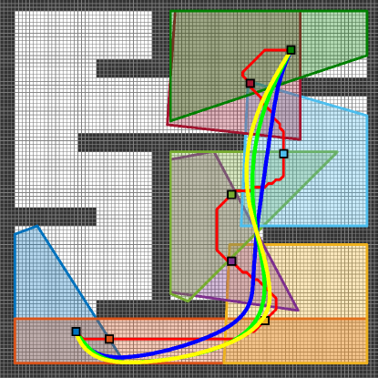
Figure 1: Graph-theoretic Bézier curve optimization aims at minimizing the consensus distance $\mathrm{tr}\mathopen{}\mathclose{{}\left({\mathbf{P}}^{\mathrm{T}}\mathbf{L}\mathbf{P}}\right)$ of control points $\mathbf{P}={[\mathrm{p}_{0},\ldots,\mathrm{p}_{n}]}^{\mathrm{T}}$ of Bézier curves $\mathrm{B}_{\mathbf{P}}(t)$ based on the positive semidefinite Laplacian matrix $\mathbf{L}$ of an interaction graph of the control points while satisfying linear equality (e.g., endpoint continuity) and inequality (e.g., safety corridor) constraints. The blue, green, and yellow curves demonstrate a collection of Bézier curves optimized over safe corridors (polygon patches) with the $C^{1}$ endpoint continuity constraint using the graph Laplacians of the (left, top) first-order difference norm, (left, middle) first-order difference variance, and (left, bottom) second-order difference norm of Bézier control points, respectively. Convex polygonal safe corridors are automatically generated using separating hyperplanes of corridor centers from obstacles around a maximal-clearance minimal-length reference path (red).

I-A Motivation and Related Literature

The quadratic nature of the squared norm of high-order derivatives of polynomial Bézier curves is a primary reason for their popularity for computationally efficient quadratic optimization in smooth motion planning and path smoothing, especially when dealing with differential flat systems [16] such as cars [7, 8], quadrotors [1, 2, 3], and fixed-wing aircraft [14], to name a few, whose control inputs can be expressed as a function of flat system outputs (represented by polynomials) and their derivatives. Most existing work on polynomial trajectory optimization mainly focuses on time-parametrized polynomials to minimize physical quadratic objective functions such as total velocity, acceleration, jerk, and snap [17, 18, 19, 15]. Inspired by spring forces and potentials, the norm of the second-order finite difference of Bézier control points, also known as the elastic band cost [20, 21], is also used as a geometric optimization objective to decouple time allocation with geometric curve optimization [22]. In all of this existing literature, although the Hessian of a quadratic optimization objective is crucial for quadratic optimization of polynomial curves, it is omitted for brevity, or, in some cases, presented through manual calculation or symbolic and numeric computation. The lack of a general explicit analytical expression for the Hessian of the optimization function obscures the relationships between potentially related optimization objectives. Consequently, it becomes challenging to intuitively understand how these objectives influence polynomial curve parameters. In this paper, we present an explicit analytical formula for the norm and variance of the high-order derivatives of Bézier curves, as well as the finite differences of Bézier control points using matrix representations and operations associated with Bézier curves. We also demonstrate that these quadratic objective functions can be unified as a consensus distance of Bézier control points, which is derived from the Laplacian matrix of a weighted interaction graph of the control points. The explicit analytical forms of the Hessian, along with their graph-theoretical interpretations, offer new insights into Bézier optimization objectives. For example, for Bézier curves of degree $n=2$, Bézier velocity norm is equivalent to the variance of the control points, and similarly, Bézier acceleration norm is equivalent to the variance of the first-order difference of the control points for $n=2,3$. We believe that our explicit matrix formulation of Bézier curve optimization can reduce the knowledge gap and make it more accessible for researchers to apply these tools effectively.

The convex nature of Bézier curves makes them an ideal choice for addressing system and task constraints as a linear inequality constraint in quadratic optimization, particularly for safe and smooth motion planning around obstacles. Since Bézier curves are contained in the convex hull of their control points, such optimization constraints are often enforced by constraining Bézier control points inside some convex constraint sets, known as safe corridors [4, 23, 24]. Safe corridors are often iteratively constructed around a reference path in various shapes, including convex polytopes [18, 25], boxes [17, 19, 4], and spheres [3, 26, 15], with the aim of maximizing their volume to limit the number of safe corridors and, consequently, the Bézier curves used in optimization. Piecewise-linear reference paths are commonly preferred due to their simple construction, e.g., using graph search methods [17, 18, 19] or sampling-based planning algorithms [26, 15, 27]. Fast marching with a distance field is applied to find a reference path that balances the distance to obstacles, facilitating the creation of maximal volume safe corridors [28, 4]. In this paper, to achieve a minimal number of safe corridors and Bézier curves, we iteratively construct maximal-volume convex polygonal safe corridors along a maximal-clearance minimal-length reference path using the separating hyperplanes of corridor centers from obstacles [18, 29, 30] where we find a maximal-clearance minimal-length reference path over a binary occupancy map using graph search with the inverse distance field as a cost map.

I-B Contributions and Organization of the Paper

In this paper, we introduce a new family of graph-theoretic quadratic Bézier optimization objectives that use a consensus distance to measure the alignment between Bézier control points based on the Laplacian of their weighted interaction graph. In Section II, we provide a brief background on Bézier curves and highlight their important analytical properties that enable an explicit matrix formulation of Bézier curve optimization. In Section III, we present a new quadratic consensus distance for Bézier control points and provide physical, geometric, and statistical consensus distance examples. In Section IV, using separating hyperplanes of obstacles, we describe a systematic and effective way of automatically constructing maximal-volume convex polygonal corridors along a reference path that balances distance to obstacles. In Section V, we present example applications of Bézier curve optimization over safe corridors using various quadratic optimization objectives. We conclude in Section VI with a summary of our contributions and future work.

II Bézier Curves

In this section, we introduce the notation used throughout the paper and provide a brief background on Bézier curves, including their important properties and matrix operations, which are essential to Bézier curve optimization in safe and smooth motion planning.

Definition 1

(Bézier Curve) In a $d$-dimensional Euclidean space $\mathbb{R}^{d}$, a Bézier curve $\mathrm{B}_{\mathrm{p}_{0},\ldots\mathrm{p}_{n}}(t)$ of degree $n\in\mathbb{N}$, associated with control points $\mathrm{p}_{0},\ldots,\mathrm{p}_{n}\in\mathbb{R}^{d}$, is a parametric $n^{\text{th}}$-order polynomial curve defined for $0\leq t\leq 1$ as

$$\mathrm{B}_{\mathrm{p}_{0},\ldots,\mathrm{p}_{n}}(t):=\sum_{i=0}^{n}b_{i,n}(t)\mathrm{p}_{i},$$ (1)

where $b_{i,n}(t)$ denotes the $i^{\text{th}}$ Bernstein basis polynomial of degree $n$ that is defined for $i=0,1,\ldots,n$ as

$$b_{i,n}(t):=\scalebox{1.2}{$\binom{n}{i}$}t^{i}(1-t)^{n-i}.$$ (2)

To effectively work with high-order Bézier curves with a large number of control points, it is convenient to use the matrix representation of Bézier curves in the form of

$$\mathrm{B}_{\mathbf{P}}(t)={\mathbf{P}}^{\mathrm{T}}\mathrm{b}_{n}(t),$$ (3)

where $\mathbf{P}\!:=\!{\mathopen{}\mathclose{{}\left[\mathrm{p}_{0},\ldots,\mathrm{p}_{n}}\right]}^{\mathrm{T}}\!\in\!\mathbb{R}^{(n+1)\times d}$ denotes the control point matrix, $\mathrm{b}_{n}(t):={\mathopen{}\mathclose{{}\left[b_{0,n}(t),\ldots,b_{n,n}(t)}\right]}^{\mathrm{T}}\in\mathbb{R}^{n+1}$ is the Bernstein basis vector of degree $n$, and ${\mathbf{A}}^{\mathrm{T}}$ denotes the transpose of a matrix $\mathbf{A}$.

Some key characteristics of Bézier and Bernstein polynomials that are important for motion planning are their interpolation, derivative, and convexity properties [31, 32, 33].

Property 1

(Interpolation) A Bézier curve, $\mathrm{B}_{\mathbf{P}}(t)$ associated with control points $\mathbf{P}={\mathopen{}\mathclose{{}\left[\mathrm{p}_{0},\ldots,\mathrm{p}_{n}}\right]}^{\mathrm{T}}$, smoothly interpolates between its first and last control points, i.e.,

$$\mathrm{B}_{\mathbf{P}}(0) ={\mathbf{P}}^{\mathrm{T}}\mathrm{b}_{n}(0)=\mathrm{p}_{0}$$ (4)

$$\mathrm{B}_{\mathbf{P}}(1) ={\mathbf{P}}^{\mathrm{T}}\mathrm{b}_{n}(1)=\mathrm{p}_{n}$$ (5)

since Bernstein basis vector $\mathrm{b}_{n}(t)={\mathopen{}\mathclose{{}\left[b_{0,n}(t),\ldots,b_{n,n}(t)}\right]}^{\mathrm{T}}$ smoothly interpolates between

$$\mathrm{b}_{n}(0)=\scalebox{0.8}{$\begin{bmatrix}1\\ 0\\ \vdots\\ 0\end{bmatrix}$}\quad\text{ and }\quad\mathrm{b}_{n}(1)=\scalebox{0.8}{$\begin{bmatrix}0\\ \vdots\\ 0\\ 1\end{bmatrix}$}.$$ (6)

The interpolation property of Bézier curves allows for describing endpoint constraints, such as start and goal positions, as a linear equality constraint in Bézier curve optimization, as illustrated in Table I.

Property 2

(High-Order Derivatives) The $k^{\text{th}}$-order derivative of a Bézier curve of degree $n$, where $k\in\mathopen{}\mathclose{{}\left\{0\ldots,n}\right\}$, is another Bézier curve of degree $(n-k)$ that is given by

$$\mathrm{B}^{(k)}_{\mathbf{P}}(t):=\frac{\mathrm{d}^{k}}{\mathrm{d}t^{k}}\mathrm{B}_{\mathbf{P}}(t) =\scalebox{0.85}{$\dfrac{n!}{(n-k)!}$}\mathrm{B}_{\mathbf{D}(n,k)\mathbf{P}}(t)$$ (7)

where $\mathbf{D}(n,k)$ denotes the $k^{\text{th}}$-order forward finite-difference matrix in $\mathbb{R}^{(n-k+1)\times(n+1)}$ whose elements are

$$\mathopen{}\mathclose{{}\left[\mathbf{D}(n,k)}\right]_{i+1,j+1}\!=\!\mathopen{}\mathclose{{}\left\{\begin{array}[]{@{}c@{}l@{}}\binom{k}{j-i}\!(-1)^{k-j+i}&\text{, if }0\leq j-i\leq k\\ 0&\text{, otherwise.}\end{array}}\right.\!$$ (10)

for $i=0,\ldots,(n-k)$ and $j=0,\ldots,n$, and the $k^{\text{th}}$-order derivative of the Bernstein basis vector $\mathrm{b}_{n}(t)$ also satisfies

$$\frac{\mathrm{d}^{k}}{\mathrm{d}t^{k}}\mathrm{b}_{n}(t)=\tfrac{n!}{(n-k)!}{\mathbf{D}(n,k)}^{\mathrm{T}}\mathrm{b}_{n-k}(t).$$ (11)

Note that, by definition, $\mathbf{D}(n,0)=\mathbf{I}$ and $\mathbf{D}(n,k)\mathbf{1}=\mathbf{0}$ for any $k=1,\ldots,n$, where $\mathbf{I}$ denotes the square identity matrix; and $\mathbf{1}$ and $\mathbf{0}$ are, respectively, the column vector of all ones and zeros of appropriate sizes. If more precision is required, we use subscripts to specify the dimensions of these matrices, for example, $\mathbf{I}_{n}$ and $\mathbf{I}_{n\times n}$ denote the $n\times n$ identity matrix whereas $\mathbf{0}_{n}$ and $\mathbf{0}_{n\times 1}$ denote the $n\times 1$ zero column vector. For the special case of the first-order Bézier derivative $\frac{\mathrm{d}}{\mathrm{d}t}\mathrm{B}_{\mathbf{P}}(t)=n\mathrm{B}_{\mathbf{D}(n,1)\mathbf{P}}(t)$,

$$\mathbf{D}(n,1)=\mathopen{}\mathclose{{}\left[\mathbf{0}_{n\times 1},\mathbf{I}_{n\times n}}\right]-\mathopen{}\mathclose{{}\left[\mathbf{I}_{n\times n},\mathbf{0}_{n\times 1}}\right]$$ (12)

which allows us to recursively determine the $k^{\text{th}}$-order forward difference matrix $\mathbf{D}(n,k)$ as

$$\mathbf{D}(n,k)=\mathbf{D}(n-1,k-1)\mathbf{D}(n,1).$$ (13)

It is important to highlight that the high-order derivative property of Bézier curves enables the expression of endpoint derivative constraints (e.g., ensuring a specific level of continuity and smoothness between adjacent Bézier curve segments as shown in Table I) as a linear equality constraint of Bézier control points as

$$\frac{\mathrm{d}^{k}}{\mathrm{d}t^{k}}\mathrm{B}_{\mathbf{P}}(0) =\tfrac{n!}{(n-k)!}{\mathbf{P}}^{\mathrm{T}}{\mathbf{D}(n,k)}^{\mathrm{T}}\mathrm{b}_{n-k}(0)$$ (14)

$$\frac{\mathrm{d}^{k}}{\mathrm{d}t^{k}}\mathrm{B}_{\mathbf{P}}(1) =\tfrac{n!}{(n-k)!}{\mathbf{P}}^{\mathrm{T}}{\mathbf{D}(n,k)}^{\mathrm{T}}\mathrm{b}_{n-k}(1).$$ (15)

TABLE I: An Explicit Matrix Formulation for Quadratic Optimization of Bézier Curves

Find the control point matrices $\mathbf{P}_{1},\ldots,\mathbf{P}_{m}\in\mathbb{R}^{(n+1)\times d}$ of $m$ Bézier curves of degree $n$ that join $\mathrm{p}_{\mathrm{start}},\mathrm{p}_{\mathrm{goal}}\in\mathbb{R}^{d}$ and minimize the total squared norm of the $k^{\text{th}}$-order derivative of Bézier curves with a certain degree $C$ of continuity under given linear inequality constraints
minimize	$\sum\limits_{i=1}^{m}\int_{0}^{1}\|\frac{\mathrm{d}^{k}}{\mathrm{d}t^{k}}\mathrm{B}_{\mathbf{P}_{i}}(t)\|^{2}\mathrm{d}t$	$\Longleftrightarrow$	$\sum\limits_{i=1}^{m}\mathrm{tr}\mathopen{}\mathclose{{}\left({\mathbf{P}_{i}}^{\mathrm{T}}{\mathbf{D}(n,k)}^{\mathrm{T}}\mathbf{H}_{\mathrm{N}}(n-k)\mathbf{D}(n,k)\mathbf{P}_{i}}\right)$
subject to	$\mathrm{B}_{\mathbf{P}_{1}}(0)=\mathrm{p}_{\mathrm{start}}$, $\mathrm{B}_{\mathbf{P}_{m}}(1)=\mathrm{p}_{\mathrm{goal}}$	$\Longleftrightarrow$	${\mathbf{P}_{1}}^{\mathrm{T}}\scalebox{0.6}{$\begin{bmatrix}1\\ 0\\ \vdots\\ 0\end{bmatrix}$}=\mathrm{p}_{\mathrm{start}}$, ${\mathbf{P}_{m}}^{\mathrm{T}}\scalebox{0.6}{$\begin{bmatrix}0\\ \vdots\\ 0\\ 1\end{bmatrix}$}=\mathrm{p}_{\mathrm{goal}}$
	$\frac{\mathrm{d}^{c}}{\mathrm{d}t^{c}}\mathrm{B}_{\mathbf{P}_{i}}(1)=\frac{\mathrm{d}^{c}}{\mathrm{d}t^{c}}\mathrm{B}_{\mathbf{P}_{i+1}}(0)\quad$ $\forall i=1,\dots,m-1$ $\forall c=0,\ldots,C$	$\Longleftrightarrow$	${\mathbf{P}_{i}}^{\mathrm{T}}{\mathbf{D}(n,c)}^{\mathrm{T}}\scalebox{0.6}{$\begin{bmatrix}0\\ \vdots\\ 0\\ 1\end{bmatrix}$}={\mathbf{P}_{i+1}}^{\mathrm{T}}{\mathbf{D}(n,c)}^{\mathrm{T}}\scalebox{0.6}{$\begin{bmatrix}1\\ 0\\ \vdots\\ 0\end{bmatrix}$}\quad$ $\forall i=1,\dots,m-1$ $\forall c=0,\ldots,C$
	$\mathbf{A}_{i}\mathrm{B}_{\mathbf{P}_{i}}(t)\leq\mathrm{b}_{i}\quad\forall t\in[0,1],\forall i=1,\dots,m-1$	$\Longleftarrow$	$\mathbf{A}_{i}{\mathbf{P}_{i}}^{\mathrm{T}}\leq\mathrm{b}_{i}{\mathbf{1}}^{\mathrm{T}}\quad\forall i=1,\dots,m-1$

Property 3

(Convexity) A Bézier curve $\mathrm{B}_{\mathbf{P}}(t)$ is defined as a continuous convex combination of its control points $\mathbf{P}={\mathopen{}\mathclose{{}\left[\mathrm{p}_{0},\ldots,\mathrm{p}_{n}}\right]}^{\mathrm{T}}$, and so it is contained in the convex hull, denoted by $\mathrm{conv}$, of the control points, i.e.,

$$\mathrm{B}_{\mathbf{P}}(t)\in\mathrm{conv}\mathopen{}\mathclose{{}\left(\mathrm{p}_{0},\ldots,\mathrm{p}_{n}}\right)\quad\quad\forall t\in[0,1],$$ (16)

because Bernstein polynomials are nonnegative and sum to one, i.e., for any $t\in[0,1]$

$$b_{i,n}(t)\geq 0,\quad\text{and}\quad\sum_{i=0}^{n}b_{i,n}(t)=1.$$ (17)

The convexity of Bézier curves allows for a simple over-approximation of linear inequality (e.g., safety) constraints of the form $\mathbf{A}\mathrm{B}_{\mathbf{P}}(t)\leq\mathrm{b}$ by $\mathbf{A}{\mathbf{P}}^{\mathrm{T}}\leq\mathrm{b}{\mathbf{1}}^{\mathrm{T}}$ in Bézier curve optimization as seen in Table I because the convexity property of Bézier curves ensures that

$$\mathbf{A}{\mathbf{P}}^{\mathrm{T}}\leq\mathrm{b}{\mathbf{1}}^{\mathrm{T}}\Longrightarrow\mathbf{A}\mathrm{B}_{\mathbf{P}}(t)\leq\mathrm{b}\quad\forall t\in[0,1].$$ (18)

Another crucial property of Bézier curves for defining quadratic optimization objectives is that the inner product of Bézier curves can be explicitly calculated as the inner product of their control points, which is mainly due to the constant definite integral property of Bernstein polynomials (i.e.,$\int_{0}^{1}b_{k,n}(t)\mathrm{d}t=\frac{1}{n+1}\quad\forall k=0,\ldots,n$).

Lemma 1

(Bézier Inner Product) The inner product of a pair of Bézier curves $\mathrm{B}_{\mathbf{P}}(t)$ and $\mathrm{B}_{\mathbf{Q}}(t)$ with associated control points $\mathbf{P}={[\mathrm{p}_{0},\ldots,\mathrm{p}_{n}]}^{\mathrm{T}}\!\in\!\mathbb{R}^{(n+1)\times d}$ and $\mathbf{Q}={[\mathrm{q}_{0},\ldots,\mathrm{q}_{m}]}^{\mathrm{T}}\!\in\!\mathbb{R}^{(m+1)\times d}$ satisfies

$$\int_{0}^{1}{\mathrm{B}_{\mathbf{P}}(t)}^{\mathrm{T}}\mathrm{B}_{\mathbf{Q}}(t)\mathrm{d}t=\mathrm{tr}\mathopen{}\mathclose{{}\left(\mathbf{P}\mathbf{H}_{\mathrm{B}}(n,m){\mathbf{Q}}^{\mathrm{T}}}\right)$$ (19)

where $\mathrm{tr}$ denotes the matrix trace operator and $\mathbf{H}_{\mathrm{B}}(n,m):=\int_{0}^{1}\mathrm{b}_{n}(t){\mathrm{b}_{m}(t)}^{\mathrm{T}}\mathrm{d}t$ is the Bernstein outer product matrix in $\mathbb{R}^{(n+1)\times(m+1)}$ whose elements are given for $i=0,\ldots,n$ and $j=0,\ldots,m$ by

$$\mathopen{}\mathclose{{}\left[\mathbf{H}_{\mathrm{B}}(n,m)}\right]_{i+1,j+1}=\tfrac{1}{m+n+1}\frac{\binom{n}{i}\binom{m}{j}}{\binom{m+n}{i+j}}.$$ (20)

Proof.

See Appendix A-A. ∎

The inner product property of Bézier curves is crucial for recognizing that the squared norm of a Bézier curve of degree $n$ is a convex quadratic function of its control points, i.e.,

$$\|\mathrm{B}_{\mathbf{P}}\|^{2}:=\int_{0}^{1}\|\mathrm{B}_{\mathbf{P}}(t)\|^{2}\mathrm{d}t=\mathrm{tr}\mathopen{}\mathclose{{}\left({\mathbf{P}}^{\mathrm{T}}\mathbf{H}_{\mathrm{N}}(n)\mathbf{P}}\right)$$ (21)

where the elements of the Hessian $\mathbf{H}_{\mathrm{N}}(n):=\mathbf{H}_{\mathrm{B}}(n,n)$ of the squared Bézier norm are given for $i,j=0,\ldots,n$ by

$$\mathopen{}\mathclose{{}\left[\mathbf{H}_{\mathrm{N}}(n)}\right]_{i+1,j+1}=\tfrac{1}{2n+1}\frac{\binom{n}{i}\binom{n}{j}}{\binom{2n}{i+j}}.$$ (22)

Note that $\mathbf{0}\!\preceq\!\mathbf{H}_{\mathrm{N}}(n)\!\preceq\!\frac{1}{n+1}\mathbf{I}$ due to Jensen’s inequality. The analytical form of the Hessian of the Bézier derivative norm, combined with Bézier matrix operations, enables an explicit and compact formulation for quadratic optimization of Bézier curves as shown in Table I.

Yet another quadratic function of Bézier curves that is crucial for Bézier curve optimization is variance.

Lemma 2

(Bézier Statistics) The mean of a Bézier curve $\mathrm{B}_{\mathbf{P}}(t)$ and the mean of its controls points $\mathbf{P}={\mathopen{}\mathclose{{}\left[\mathrm{p}_{0},\ldots,\mathrm{p}_{n}}\right]}^{\mathrm{T}}$ are the same, whereas the variance of the Bézier curve is tightly bounded above by the variance of the control points as

$$\mu(\mathrm{B}_{\mathbf{P}})=\mu(\mathbf{P})\,\text{ and }\,\sigma^{2}(\mathrm{B}_{\mathbf{P}})\leq\tfrac{1}{n+1}\sigma^{2}(\mathbf{P})$$ (23)

where the overloaded mean and variance operators for both Bézier curves and Bézier control points are defined as^II

$$\!\!\mu(\mathrm{B}_{\mathbf{P}}) \!:=\!\!\int\limits_{0}^{1}\!\mathrm{B}_{\mathbf{P}}(t)\mathrm{d}t,\!\!\! \!\!\!\sigma^{2}(\mathrm{B}_{\mathbf{P}}) \!:=\!\int\limits_{0}^{1}\|\mathrm{B}_{\mathbf{P}}(t)-\mu(\mathrm{B}_{\mathbf{P}})\|^{2}\mathrm{d}t$$

$$\!\!=\mathrm{tr}\mathopen{}\mathclose{{}\left({\mathbf{P}}^{\mathrm{T}}\mathbf{S}(n)\mathbf{H}_{\mathrm{N}}(n)\mathbf{S}(n)\mathbf{P}}\right),$$

$$\!\!\mu(\mathbf{P}) \!:=\!\tfrac{1}{n+1}\!\sum_{i=0}^{n}\mathrm{p}_{i}, \sigma^{2}(\mathbf{P}) \!:=\!\tfrac{1}{n+1}\sum_{i=0}^{n}\|\mathrm{p}_{i}-\overline{\mu}(\mathrm{B}_{\mathbf{P}})\|^{2}$$

$$=\tfrac{1}{n+1}\mathrm{tr}\mathopen{}\mathclose{{}\left({\mathbf{P}}^{\mathrm{T}}\mathbf{S}(n)\mathbf{P}}\right)$$ (24)

in terms of the Bézier norm Hessian $\mathbf{H}_{\mathrm{N}}(n)$ in (22) and the mean-shift matrix $\mathbf{S}(n)$ that is defined to be

$$\mathbf{S}(n):=\mathbf{I}_{n+1}-\tfrac{1}{n+1}\mathbf{1}_{n+1}{\mathbf{1}}^{\mathrm{T}}_{n+1}.$$ (25)

Proof.

See Appendix A-B. ∎

It is useful to observe that the mean-shift matrix is a projection operator, i.e., $\mathbf{S}(n)\mathbf{S}(n)=\mathbf{S}(n)$, that is symmetric and positive semidefinite, and it satisfies $\mathbf{S}(n)\mathbf{1}=\mathbf{0}$.

III ​​ Graph-Theoretic Bézier Optimization Objective​

In this section, we introduce a new consensus-based quadratic Bézier optimization objective that is designed to assess the agreement and alignment of Bézier control points based on the Laplacian matrix of their interaction graph. We present example physical, geometric, and statistical consensus-based optimization objectives that are constructed based on differential norms and variances.

III-A Consensus-Based Bézier Optimization Objective

A Bézier curve is, by definition, constructed based on a continuous convex combination of its control points to smoothly interpolate and connect its first and last control points (see Definition 1, Property 1, and Property 3). Hence, the shape of a Bézier curve (whether it is straight or oscillatory) is completely determined by its control points. A smooth and high-quality Bézier curve that satisfies a set of given geometric (e.g., boundary, length, intersection) conditions requires a certain level of agreement or alignment between its control points. Accordingly, inspired by consensus in networked multi-agent systems [34], to determine the agreement of control points of a Bézier curve, we assume that Bézier control points interact over a weighted undirected connected graph (without self loops) specified by a positive semidefinite Laplacian matrix $\mathbf{L}\in S_{+}^{n+1}$ with $\mathbf{L}\mathbf{1}=0$, where the interaction weights $\mathbf{W}\in\mathbb{R}^{(n+1)\times(n+1)}$ between the control points for $i,j=0,\ldots,n$ are given by

$$\mathopen{}\mathclose{{}\left[\mathbf{W}}\right]_{i+1,j+1}=\mathopen{}\mathclose{{}\left\{\begin{array}[]{@{}cl@{}}0&\text{ if }i=j\\ -[\mathbf{L}]_{i+1,j+1}&\text{ otherwise.}\end{array}}\right.$$ (28)

Note that an interaction weight between a pair of control points might be positive or negative. A positive interaction weight signifies similarity among control points, whereas a negative interaction weight promotes divergence or dissimilarity among control points. Accordingly, as a new unifying Bézier curve optimization objective, we consider a common measure of distance from consensus [34] that is defined based on the interaction graph Laplacian as follows.

Definition 2

(Bézier Consensus Distance) Given a symmetric and positive semidefinite interaction graph Laplacian $\mathbf{L}\in S_{+}^{n+1}$ with $\mathbf{L}\mathbf{1}=\mathbf{0}$, the consensus distance, denoted by $\mathcal{C}_{\mathbf{L}}$, of the control points $\mathbf{P}\in\mathbb{R}^{(n+1)\times d}$ of a Bézier curve $\mathrm{B}_{\mathbf{P}}(t)$ is a measure of disagreement of the control points that is quantified as $\mathcal{C}_{\mathbf{L}}(\mathbf{P}):=\mathrm{tr}\mathopen{}\mathclose{{}\left({\mathbf{P}}^{\mathrm{T}}\mathbf{L}\mathbf{P}}\right)$.

The singularity of graph Laplacian, i.e., $\mathbf{L}\mathbf{1}\!=\!\mathbf{0}$, implies that the consensus distance of Bézier control points is determined by the relative differences of the control points rather than absolute control point locations. For a connected interaction graph with positive weights (i.e., the graph Laplacian has exactly one zero-eigenvalue), the perfect consensus of Bézier control points (i.e., $\mathrm{tr}\mathopen{}\mathclose{{}\left({\mathbf{P}}^{\mathrm{T}}\mathbf{L}\mathbf{P}}\right)=0$) means a constant Bézier curve (i.e., $\mathrm{B}_{\mathbf{P}}(t)=\mathrm{p}$ since $\mathbf{P}={\mathopen{}\mathclose{{}\left[\mathrm{p},\ldots,\mathrm{p}}\right]}^{\mathrm{T}}$), which corresponds to zero motion at $\mathrm{p}$. In Table II, we present example physical, geometric, and statistical consensus distances for Bézier curve optimization whose graph-theoretic interpretation is illustrated in Table III and discussed below.

III-B Physical Bézier Optimization Objectives

In polynomial trajectory optimization, a widely-used physical optimization objective is the squared norm of Bézier derivatives, for example, to minimize total velocity, acceleration, jerk, snap and their various combinations.

Proposition 1

(Bézier Derivative Norm) The squared norm of $k^{\text{th}}$-order derivative of an $n^{\text{th}}$-order Bézier curve associated with control point matrix $\mathbf{P}\in\mathbb{R}^{(n+1)\times d}$ is given by

$$\int_{0}^{1}\|\tfrac{\mathrm{d}^{k}}{\mathrm{d}t^{k}}\mathrm{B}_{\mathbf{P}}(t)\|^{2}\mathrm{d}t=\frac{n!^{2}}{(n-k)!^{2}}\mathrm{tr}\mathopen{}\mathclose{{}\left({\mathbf{P}}^{\mathrm{T}}\mathbf{H}_{\mathrm{DN}}(n,k)\mathbf{P}}\right)$$ (29)

where the Hessian $\mathbf{H}_{\mathrm{DN}}(n,k)$ of Bézier derivative norm

$$\mathbf{H}_{\mathrm{DN}}(n,k):={\mathbf{D}(n,k)}^{\mathrm{T}}\mathbf{H}_{\mathrm{N}}(n-k)\mathbf{D}(n,k)$$ (30)

is determined by the high-order finite-difference matrix $\mathbf{D}(n,k)$ in (10) and the Bézier norm Hessian $\mathbf{H}_{\mathrm{N}}(n)$ in (22).

Proof.

The statement is a consequence of the derivative and inner-product properties of Bézier curves in Property 2 and Lemma 1, respectively, i.e., $\tfrac{\mathrm{d}^{k}}{\mathrm{d}t^{k}}\mathrm{B}_{\mathbf{P}}(t)=\frac{n!}{(n-k)!}\mathrm{B}_{\mathbf{D}(n,k)\mathbf{P}}(t)$ and $\int_{0}^{1}\|\mathrm{B}_{\mathbf{P}}(t)\|^{2}\mathrm{d}t=\mathrm{tr}\mathopen{}\mathclose{{}\left({\mathbf{P}}^{\mathrm{T}}\mathbf{H}_{\mathrm{N}}(n)\mathbf{P}}\right)$. ∎

Note that $\mathbf{H}_{\mathrm{DN}}(n,k)={\mathbf{D}(n,k)}^{\mathrm{T}}\mathbf{H}_{\mathrm{N}}(n-k)\mathbf{D}(n,k)$ is a symmetric and positive semidefinite matrix and satisfies $\mathbf{H}_{\mathrm{DN}}(n,k)\mathbf{1}=\mathbf{0}$ for $k=1,\ldots,n$ because $\mathbf{H}_{\mathrm{N}}(n-k)$ is positive definite and $\mathbf{D}(n,k)\mathbf{1}=\mathbf{0}$. Hence, from a graph-theoretic perspective, one may consider the Hessian $\mathbf{H}_{\mathrm{DN}}(n,k)$ of Bézier derivative norm as a graph Laplacian matrix to better understand the interaction relation between Bézier control points. In Table III, we illustrate the weighted interaction graphs of Bézier control points corresponding to Bézier velocity and acceleration norms using the associated Hessian matrices $\mathbf{H}_{\mathrm{DN}}(n,1)$ and $\mathbf{H}_{\mathrm{DN}}(n,2)$ for $n=2,3,4$.

TABLE II: Example Consensus-Based Bézier Optimization Objectives

Objection Function	Consensus Distance
Control-Point Difference Norm $\|\mathbf{D}(n,k)\mathbf{P}\|^{2}$	$\mathrm{tr}\mathopen{}\mathclose{{}\left({\mathbf{P}}^{\mathrm{T}}{\mathbf{D}(n,k)}^{\mathrm{T}}\mathbf{D}(n,k)\mathbf{P}}\right)$
Bézier Derivative Norm $\|\mathrm{B}_{\mathbf{D}(n,k)\mathbf{P}}\|^{2}$	$\mathrm{tr}\mathopen{}\mathclose{{}\left({\mathbf{P}}^{\mathrm{T}}{\mathbf{D}(n,k)}^{\mathrm{T}}\mathbf{H}_{\mathrm{N}}(n\!-\!k)\mathbf{D}(n,k)\mathbf{P}}\right)$
Control-Point Difference Variance $\sigma^{2}\mathopen{}\mathclose{{}\left(\mathbf{D}(n,k)\mathbf{P}}\right)$	$\mathrm{tr}\mathopen{}\mathclose{{}\left({\mathbf{P}}^{\mathrm{T}}{\mathbf{D}(n,k)}^{\mathrm{T}}\mathbf{S}(n\!-\!k)\mathbf{D}(n,k)\mathbf{P}}\right)$
Bézier Derivative Variance $\sigma^{2}\mathopen{}\mathclose{{}\left(\mathrm{B}_{\mathbf{D}(n,k)\mathbf{P}}}\right)$	$\mathrm{tr}\mathopen{}\mathclose{{}\left(\!{\mathbf{P}}^{\mathrm{T}}{\mathbf{D}(n,k)\!}^{\mathrm{T}}\mathbf{S}(n\!-\!k)\mathbf{H}_{\mathrm{N}}(n\!-\!k)\mathbf{S}(n\!-\!k)\mathbf{D}(n,k)\mathbf{P}\!}\right)\!$

III-C Geometric Bézier Optimization Objectives

Replacing continuous differentiation with finite differencing often yields geometrically more intuitive Bézier optimization objectives. More specifically, instead of Bézier derivative norm $\int_{0}^{1}\|\frac{\mathrm{d}^{k}}{\mathrm{d}t^{k}}\mathrm{B}_{\mathbf{P}}(t)\|\mathrm{d}t$, as a geometric optimization objective, we consider the squared norm of finite difference of Bézier control points that is given by

$$\|\mathbf{D}(n,k)\mathbf{P}\|^{2}=\mathrm{tr}\mathopen{}\mathclose{{}\left({\mathbf{P}}^{\mathrm{T}}\mathbf{H}_{\overline{\mathrm{DN}}}(n,k)\mathbf{P}}\right)$$ (31)

where the Hessian $\mathbf{H}_{\overline{\mathrm{DN}}}(n,k)$ of Bézier control-point difference norm is defined in terms of the finite-difference matrix $\mathbf{D}(n,k)$ in (10) as

$$\mathbf{H}_{\overline{\mathrm{DN}}}(n,k):={\mathbf{D}(n,k)}^{\mathrm{T}}\mathbf{D}(n,k).$$ (32)

In Table III, we present the corresponding interaction graphs of the first-order and second-order difference norm of Bézier control points. As seen in Table III, as a special case of $n=2$, the second-order difference and derivative norms define the same interaction relation between the control points. However, the finite-difference norm of Bézier control points often results in reduced interaction between control points compared to the Bézier derivative norm, which allows for an intuitive interpretation of geometric optimization objectives. Below, we present the explicit forms of the norm of the first- and second-order differences of control points to illustrate the geometric intuition behind the corresponding Bézier optimization objectives.

The first-order difference norm of Bézier control points defines an upper bound on the squared length of the Bézier (control) polygon that connects Bézier control points with straight lines from the first control point to the last control point, i.e.,

$$\|\mathbf{D}(n,1)\mathbf{P}\|^{2} =\sum_{k=1}^{n}\|\mathrm{p}_{k}\!-\!\mathrm{p}_{k-1}\|^{2}\geq\frac{1}{n}\mathopen{}\mathclose{{}\left(\sum_{k=1}^{n}\|\mathrm{p}_{k}\!-\!\mathrm{p}_{k-1}\|\!}\right)^{\!2}$$

where the inequality follows from Jensen’s inequality.

The second-order Bézier difference norm measures the total quadratic inequality gap between three consecutive Bézier control points, i.e.,

$$\|\mathbf{D}(n,k)\mathbf{P}\|^{2} =\sum_{i=1}^{n-1}\|\mathrm{p}_{i+1}\!-\!2\mathrm{p}_{i}\!+\!\mathrm{p}_{i-1}\|^{2}$$

$$=\sum_{i=1}^{n-1}2\|\mathrm{p}_{i+1}\!-\!\mathrm{p}_{i}\|^{2}\!+\!2\|\mathrm{p}_{i}\!-\!\mathrm{p}_{i-1}\|^{2}-\|\mathrm{p}_{i+1}\!-\!\mathrm{p}_{i-1}\|^{2}$$

where $\|\mathrm{p}_{i+1}-\mathrm{p}_{i-1}\|^{2}\leq 2\|\mathrm{p}_{i+1}-\mathrm{p}_{i}\|^{2}+2\|\mathrm{p}_{i}-\mathrm{p}_{i-1}\|^{2}$ is known as the quadratic inequality that is tight if and only if $\mathrm{p}_{k}$ is the midpoint of $\mathrm{p}_{k+1}$ and $\mathrm{p}_{k-1}$. Hence, the second-order Bézier difference norm measures the homogeneity (i.e., the linearity and uniformity) of control points and aims at uniformly placing control points along a straight line.

TABLE III: Graph-Theoretic Optimization Objectives
and Interaction Graphs^III-C of Bézier Control Points

First-Order Derivative Norm $\mathrm{tr}\mathopen{}\mathclose{{}\left({\mathbf{P}}^{\mathrm{T}}\mathbf{H}_{\mathrm{DN}}(n,1)\mathbf{P}}\right)$
First-Order Difference Norm $\sum\limits_{i=1}^{n}\|\mathrm{p}_{i}-\mathrm{p}_{i-1}\|^{2}$ $\mathrm{tr}\mathopen{}\mathclose{{}\left({\mathbf{P}}^{\mathrm{T}}\mathbf{H}_{\overline{\mathrm{DN}}}(n,1)\mathbf{P}}\right)$
Zeroth-Order Difference Variance $\sum\limits_{i=0}^{n}\sum\limits_{j=0}^{n}\frac{1}{2}\|\mathrm{p}_{i}-\mathrm{p}_{j}\|^{2}$ $\mathrm{tr}\mathopen{}\mathclose{{}\left({\mathbf{P}}^{\mathrm{T}}\mathbf{H}_{\overline{\mathrm{DV}}}(n,0)\mathbf{P}}\right)$
Second-Order Derivative Norm $\mathrm{tr}\mathopen{}\mathclose{{}\left({\mathbf{P}}^{\mathrm{T}}\mathbf{H}_{\mathrm{DN}}(n,2)\mathbf{P}}\right)$
Second-Order Difference Norm $\sum\limits_{i=1}^{n-1}\|\mathrm{p}_{i+1}-2\mathrm{p}_{i}+\mathrm{p}_{i-1}\|^{2}$ $\mathrm{tr}\mathopen{}\mathclose{{}\left({\mathbf{P}}^{\mathrm{T}}\mathbf{H}_{\overline{\mathrm{DN}}}(n,2)\mathbf{P}}\right)$
First-Order Difference Variance $\sum\limits_{i=1}^{n}n\|\mathrm{p}_{i}-\mathrm{p}_{i-1}\|^{2}-\|\mathrm{p}_{n}-\mathrm{p}_{0}\|^{2}$ $\mathrm{tr}\mathopen{}\mathclose{{}\left({\mathbf{P}}^{\mathrm{T}}\mathbf{H}_{\overline{\mathrm{DV}}}(n,1)\mathbf{P}}\right)$

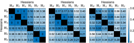
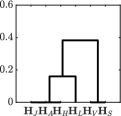
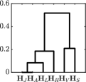
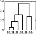
(a)                           (b)                           (c)	(d)	(e)	(f)

Figure 2: The pairwise distances of the normalized Hessians^III-D of physical, geometric, and statistical Bézier optimization objectives for (a) $n=2$, (b) $n=3$, and (c) $n=4$, and their respective complete-linkage clustering dendrograms in (d), (e), and (f). Here, $\mathbf{H}_{V}(n):=\mathbf{H}_{\mathrm{DN}}(n,1)$ and $\mathbf{H}_{A}(n):=\mathbf{H}_{\mathrm{DN}}(n,2)$ denote the physical Bézier velocity and acceleration norms; $\mathbf{H}_{L}(n):=\mathbf{H}_{\overline{\mathrm{DN}}}(n,1)$ and $\mathbf{H}_{H}(n):=\mathbf{H}_{\overline{\mathrm{DN}}}(n,2)$ denote the geometric Bézier length and homogeneity objectives defined as the first-order and the second-order finite-difference norms of the control points; and $\mathbf{H}_{S}(n):=\mathbf{H}_{\overline{\mathrm{DV}}}(n,0)$ and $\mathbf{H}_{J}(n):=\mathbf{H}_{\overline{\mathrm{DV}}}(n,1)$ denote the control-point variance and Jensen gap objectives defined as the zeroth-order and first-order finite-difference variances.

III-D Statistical Bézier Optimization Objectives

Minimizing $k^{\text{th}}$-order Bézier derivative (or difference) norm indirectly aims to minimize variation in the $(k-1)^{\text{th}}$-order Bézier derivative (or difference). Accordingly, inspired by this observation, we propose the differential variance of Bézier curves as a statistical optimization objective.

Definition 3

(Bézier Differential Variance) The differential variance of a Bézier curve can be measured using the variance of its $k^{\text{th}}$-order derivative or the variance of the $k^{\text{th}}$-order finite difference of its control points as

$$\sigma^{2}\mathopen{}\mathclose{{}\left(\mathrm{B}^{(k)}_{\mathbf{P}}}\right) =\tfrac{n!^{2}}{(n-k)!^{2}}\sigma^{2}\mathopen{}\mathclose{{}\left(\mathrm{B}_{\mathbf{D}(n,k)\mathbf{P}}}\right)$$ (33)

$$=\tfrac{n!^{2}}{(n-k)!^{2}}\mathrm{tr}\mathopen{}\mathclose{{}\left({\mathbf{P}}^{\mathrm{T}}\mathbf{H}_{\mathrm{DV}}(n,k)\mathbf{P}}\right)$$ (34)

$$\sigma^{2}\mathopen{}\mathclose{{}\left(\mathbf{D}(n,k)\mathbf{P}}\right) =\tfrac{1}{n-k+1}\mathrm{tr}\mathopen{}\mathclose{{}\left({\mathbf{P}}^{\mathrm{T}}\mathbf{H}_{\overline{\mathrm{DV}}}(n,k)\mathbf{P}}\right)$$ (35)

where the Hessians of the variances of Bézier derivatives and Bézier control-point differences are, respectively, given in terms of the difference matrix $\mathbf{D}(n,k)$ in (10) and the mean-shift matrix $\mathbf{S}(n)$ in (25) by

$$\mathbf{H}_{\mathrm{DV}}(n,k) :={\mathbf{D}(n,k)\!}^{\mathrm{T}}\mathbf{S}(n\!-\!k)\mathbf{H}_{\mathrm{N}}(n\!-\!k)\mathbf{S}(n\!-\!k)\mathbf{D}(n,k)$$

$$\mathbf{H}_{\overline{\mathrm{DV}}}(n,k) :={\mathbf{D}(n,k)\!}^{\mathrm{T}}\mathbf{S}(n\!-\!k)\mathbf{D}(n,k).$$ (36)

In Table III, we present the interaction graphs of Bézier control points for the variance of the zeroth-order and the first-order finite difference of Bézier control points using the Hessian of Bézier difference variance as the graph Laplacian. As seen in Table III, both the variance and norm of the finite difference of Bézier control points offer a simpler, reduced interaction relation between the control points compared to Bézier derivative norm and variance. We also observe that the interaction graph of the second-order derivative norm and the first-order difference variance of Bézier curves are the same for the special cases of $n=2$ and $n=3$. Hence, we find it useful to present below the explicit form of the first-order difference variance of Bézier curves to gain a better intuitive understanding of this optimization objective.

The first-order difference variance of Bézier control points measures Jensen gap of a Bézier curve that defines an upper bound on the gap between Bézier polygon length and the Euclidean distance between the first and last control point as^II

$$\sigma^{2}(\mathbf{D}(n,1)\mathbf{P}) =\tfrac{1}{n}\mathrm{tr}\mathopen{}\mathclose{{}\left({\mathbf{P}}^{\mathrm{T}}{\mathbf{D}(n,1)}^{\mathrm{T}}\mathbf{S}(n-1)\mathbf{D}(n,1)\mathbf{P}}\right)$$

$$=\tfrac{1}{n}\sum_{i=1}^{n}\sum_{j=1}^{n}\tfrac{1}{2}\|\mathrm{p}_{i}-\mathrm{p}_{i-1}-\mathrm{p}_{j}+\mathrm{p}_{j-1}\|^{2}$$

$$=\sum_{i=1}^{n}n\|\mathrm{p}_{i}-\mathrm{p}_{i-1}\|^{2}-\|\mathrm{p}_{n}-\mathrm{p}_{0}\|^{2}$$

$$\geq\mathopen{}\mathclose{{}\left(\sum_{i=1}^{n}\|\mathrm{p}_{i}-\mathrm{p}_{i-1}\|}\right)^{\!\!2}\!-\|\mathrm{p}_{n}-\mathrm{p}_{0}\|^{2}\geq 0.$$

Finally, to demonstrate the similarity and hierarchical relation among different physical, geometric, and statistical Bézier optimization objectives, we present in Fig. 2 the pairwise distance matrix of the normalized Hessians of Bézier differential norms and variances, as well as the associated clustering dendrograms, for $n=2,3,4$. As expected, the second-order (respectively, first-order) differential norms and the first-order (respectively, zeroth-order) differential variances are strongly related to each other since minimizing the acceleration norm is similar to minimizing velocity variation.

IV ​​Safe Corridors for Bézier Curve Optimization​

Safe corridors are of significant importance in defining inequality constraints within Bézier curve optimization. In this section, we present a method for constructing convex polygonal safe corridors around a reference path that heuristically balances its distance to obstacles.

IV-A Safe Corridor Construction

For motion planning around obstacles, we consider a known closed set of obstacles, denoted by $\mathcal{O}\subset\mathbb{R}^{d}$, and the associated open obstacle-free space $\mathcal{F}:=\mathbb{R}^{d}\setminus\mathcal{O}$. Modelling and understanding the connectivity and topology of free space can be challenging in motion planning [35]. Identifying a local convex free space, also referred to as a safe corridor, around a safe point in $\mathcal{F}$ allows for the exploitation of the local geometry of the free space in robot motion planning and control [29, 30]. Accordingly, we consider convex polygonal safe corridors that enable describing local safety requirements as linear inequality constraints in Bézier curve optimization.

Definition 4

(Safe Corridor) A safe corridor $\mathcal{SC}(\mathrm{c},\mathbf{X})$, parametrized by a center point $\mathrm{c}\in\mathbb{R}^{d}$ and a finite set of critical boundary points $\mathbf{X}=\mathopen{}\mathclose{{}\left(\mathrm{x}_{1},\ldots,\mathrm{x}_{m}}\right)\in\mathbb{R}^{m\times d}$ is a convex polygonal local free space in $\mathcal{F}$ that is defined using the separating hyperplanes passing through the critical boundary points $\mathbf{X}$ and facing towards the center $\mathrm{c}$ as

$$\mathcal{SC}(\mathrm{c},\mathbf{X}) \!:=\!\mathopen{}\mathclose{{}\left\{\mathrm{x}\in\mathbb{R}^{d}\Big{|}{(\mathrm{x}\!-\!\mathrm{x}_{i})\!}^{\mathrm{T}}(\mathrm{c}\!-\!\mathrm{x}_{i})\geq 0\quad\forall i=1,\ldots,m}\right\}$$

$$=\mathopen{}\mathclose{{}\left\{\mathrm{x}\!\in\mathbb{R}^{d}\big{|}{(\mathrm{x}_{i}\!-\!\mathrm{c})\!}^{\mathrm{T}}\mathrm{x}\leq{(\mathrm{x}_{i}\!-\!\mathrm{c})\!}^{\mathrm{T}}\mathrm{x}_{i}\quad\forall i=1,\ldots,m}\right\}$$

such that the corridor interior, denoted by $\mathring{\mathcal{SC}}(\mathrm{c},\mathbf{X})$, does not intersect the obstacle set, i.e., $\mathring{\mathcal{SC}}(\mathrm{c},\mathbf{X})\cap\mathcal{O}=\varnothing$.

Hence, a safe corridor can be alternatively expressed as

$$\mathcal{SC}(\mathrm{c},\mathbf{X}) =\mathopen{}\mathclose{{}\left\{\mathrm{x}\in\mathbb{R}^{d}\big{|}\mathbf{A}_{\mathcal{SC}(\mathrm{c},\mathbf{X})}\mathrm{x}\leq\mathrm{b}_{\mathcal{SC}(\mathrm{c},\mathbf{X})}}\right\}$$ (37)

where the linear inequality parameters of the safe corridor are determined by the corridor center $\mathrm{c}$ and the critical boundary points $\mathbf{X}=\mathopen{}\mathclose{{}\left(\mathrm{x}_{1},\ldots,\mathrm{x}_{m}}\right)$ as

$$\!\!\mathbf{A}_{\mathcal{SC}(\mathrm{c},\mathbf{X})}\!:=\!\begin{bmatrix}{(\mathrm{x}_{1}\!-\!\mathrm{c})}^{\mathrm{T}}\\ \vdots\\ {(\mathrm{x}_{m}\!-\!\mathrm{c})}^{\mathrm{T}}\end{bmatrix},\,\mathrm{b}_{\mathcal{SC}(\mathrm{c},\mathbf{X})}\!:=\!\begin{bmatrix}{(\mathrm{x}_{1}\!-\!\mathrm{c})}^{\mathrm{T}}\mathrm{x}_{1}\\ \vdots\\ {(\mathrm{x}_{m}\!-\!\mathrm{c})}^{\mathrm{T}}\mathrm{x}_{n}\end{bmatrix}.\!\!\!$$ (38)

One can construct a maximal-volume local free space around a given corridor centroid $\mathrm{c}$ by incrementally identifying and eliminating the closest obstacle points using separating hyperplanes, as illustrated in Fig. 3. Given any nonempty obstacle set $\mathcal{O}$ and any desired collision-free corridor center $\mathrm{c}\in\mathcal{F}$ with $\min_{\mathrm{x}_{\mathcal{O}}\in\mathcal{O}}\|\mathrm{c}-\mathrm{x}_{\mathcal{O}}\|>0$, the critical boundary points $\mathbf{X}$ of the maximal-volume safe corridor that is centered at $\mathrm{c}$ can be incrementally determined as follows:

1. (Initialize) Start with the empty boundary point set, i.e.,

   $$\mathbf{X}\leftarrow\varnothing$$

2. (Update) Find the closest point of the obstacle set in the corridor interior to the corridor center, and then add it to the critical boundary point set,

   $$\mathrm{x}^{*} =\operatornamewithlimits{arg\ min}_{\mathrm{x}_{\mathcal{O}}\in\mathcal{O}\cap\mathring{\mathcal{SC}}(\mathrm{c},\mathbf{X})}\|\mathrm{x}_{\mathcal{O}}-\mathrm{c}\|$$

   $$\mathbf{X} \leftarrow\mathbf{X}\cup\mathopen{}\mathclose{{}\left\{\mathrm{x}^{*}}\right\}$$

3. (Terminate) If $\mathring{\mathcal{SC}}(\mathrm{c},\mathbf{X})\cap\mathcal{O}\neq\varnothing$, then go to step ii. Otherwise, terminate with the boundary point set $\mathbf{X}$.

Note that this way of identifying safe corridor boundary points defines a well-defined functional relation for safe corridor construction, denoted by $f_{\mathcal{SC}}(\mathrm{p},\mathcal{O})$. Moreover, the safe corridor construction function $f_{\mathcal{SC}}(\mathrm{p},\mathcal{O})$ always returns critical corridor boundary points that define nonredundant linear inequality constraints. It is also pertinent to mention that if the obstacle set consists of a finite collection of discrete points or convex sets, then the critical boundary point set is finite because $\mathbf{X}$ might contain a boundary point corresponding to each discrete obstacle point or convex obstacle set. For example, standard point cloud sensors provide information about discrete obstacle points whereas binary occupancy grid maps represent obstacles using square-shaped occupied grid cells. To efficiently compute a safe corridor using a finite collection of obstacle points, one can start sorting the obstacle points according to their distances to the corridor center so that the search for the relevant closest obstacle point in the update step can be performed by recursively eliminating obstacle points outside the corridor. To construct a safe corridor over a binary occupancy grid map, one can employ the grid structure to perform a circular spiral search, effectively determining all relevant critical boundary points without the need to explore the entire map.

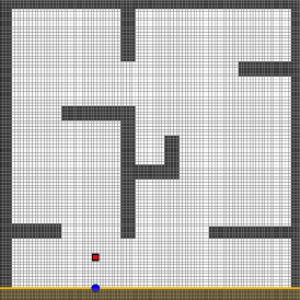
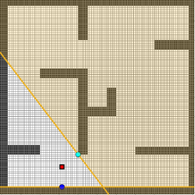
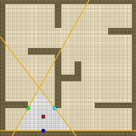
Figure 3: Construction of a convex polygonal safe corridor around a given corridor center (red square) using separating hyperplanes from obstacles.

An important application of safe corridors is identifying the available local free space around a given reference path. To minimize the number of safe corridors along the reference path, one can begin by placing a safe corridor at the start of the reference path and then incrementally search for the next reference path point to position the subsequent safe corridor center. Here, the search constraint is that the path segment between the previous and next corridor centers must stay within the previous safe corridor Accordingly, given a collision-free reference path $\mathrm{r}:[0,1]\rightarrow\mathcal{F}$ with some positive clearance from obstacles, i.e., $\min_{\begin{subarray}{c}t\in[0,1]\\ \mathrm{x}_{\mathcal{O}}\in\mathcal{O}\end{subarray}}\|\mathrm{r}(t)-\mathrm{x}_{\mathcal{O}}\|>0$, we construct a sequence of adjacent safe corridors with intersections as illustrated in Fig. 4 and described below:

1. (Initialize) Construct a safe corridor at the start of the reference path: for $k\leftarrow 1$

   $$t_{k} \leftarrow 0$$

   $$\mathbf{X}_{k} \leftarrow f_{\mathcal{SC}}(\mathrm{r}[t_{k}],\mathcal{O})$$

2. (Update) Find the reference path point that is furthest from the previous corridor center, ensuring that the associated reference path segment remains within the previous safe corridor, and construct a safe corridor at this next reference path point: for $k\leftarrow k+1$

   $$t_{k} =\operatornamewithlimits{arg\ max}_{\begin{subarray}{c}t\in[t_{k-1},1]\\ r([t_{i-1},t])\subseteq\mathcal{SC}\mathopen{}\mathclose{{}\left(r(t_{i-1}),\mathbf{X}_{i-1}}\right)\end{subarray}}t$$

   $$\mathbf{X}_{k} \leftarrow f_{\mathcal{SC}}(\mathrm{r}[t_{k}],\mathcal{O})$$

3. (Terminate) If $t_{k}<1$, then go to step ii. Otherwise, terminate with the safe corridor centers $\mathopen{}\mathclose{{}\left(\mathrm{r}(t_{1}),\ldots,\mathrm{r}(t_{k})}\right)$ and the critical boundary points $\mathopen{}\mathclose{{}\left(\mathbf{X}_{1},\ldots,\mathbf{X}_{k}}\right)$.

Note that the number and size of safe corridors constructed around a reference path depend primarily on the reference path’s clearance from obstacles and its length. A shorter reference path with greater clearance results in fewer and larger safe corridors.

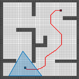
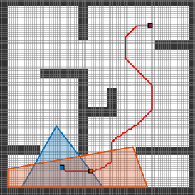
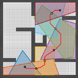
Figure 4: Construction of safe corridors along a safe reference path (red line) from the start (blue square) to the goal (red square).

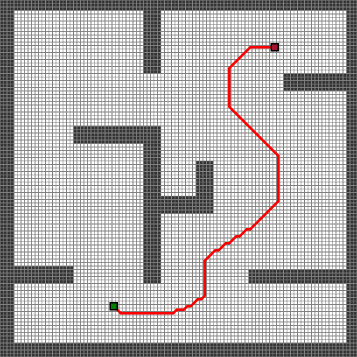
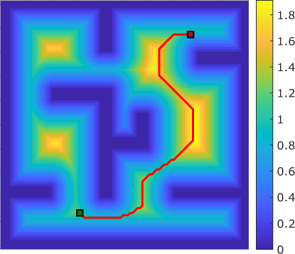
Figure 5: A maximal-clearance minimal-length reference path over a binary grid map (left) is constructed using graph search with the inverse of the distance field (right) as a cost map to balance clearance from obstacles.

IV-B Reference Path Planning for Safe Corridor Construction

To minimize the number of safe corridors and maximize their volume, we adopt a heuristic reference path construction strategy that maximizes clearance from obstacles while simultaneously minimizing the length of the reference path. In particular, to find a reference path with maximal clearance and minimal length over a binary occupancy grid map, we utilize the inverse distance field, representing the inverse of the distance to collision, as the visiting cost for each map grid cell, i.e.,

$$\mathrm{cost}(\mathrm{grid})=\frac{1}{\mathrm{dist2coll}(\mathrm{grid})}.$$

We then determine the minimum-cost path joining a given pair of start and goal positions, using a graph search (e.g., A* or Dijkstra) algorithm over a binary occupancy map (assuming 8-neighbor connectivity) where the edge transition cost between two adjacent grid cells is set as the maximum of their individual visiting costs, i.e.,

$$\mathrm{travel\_cost}(\mathrm{grid}_{i},\mathrm{grid}_{j}) =\max\mathopen{}\mathclose{{}\left(\mathrm{cost}(\mathrm{grid}_{i}),\mathrm{cost}(\mathrm{grid}_{j})}\right)$$

$$=\frac{1}{\min\mathopen{}\mathclose{{}\left(\mathrm{dist2coll}(\mathrm{grid}_{i}),\mathrm{dist2coll}(\mathrm{grid}_{j})}\right)}.$$

In Fig. 5, we illustrate an example of a maximal-clearance minimal-length reference path over a binary occupancy grid map that connects a given start and goal positions while ensuring a balanced distance from nearby obstacles.

V Numerical Simulations

In this section, we present numerical examples to demonstrate graph-theoretic Bézier curve optimization over safe corridors on a binary occupancy map using different physical, geometric and statistical Bézier optimization objectives. For a given start and goal positions, denoted by $\mathrm{p}_{\mathrm{start}}$ and $\mathrm{p}_{\mathrm{goal}}$, we first find a maximal-clearance minimal-length reference path joining $\mathrm{p}_{\mathrm{start}}$ and $\mathrm{p}_{\mathrm{goal}}$ as described in Section IV-B. Then, we automatically deploy a collection of safe corridors, denoted by $\mathcal{SC}_{1},\ldots,\mathcal{SC}_{m}$, along the reference path as described in Section IV-A.

We assume that each safe corridor is associated with a Bézier curve for which it defines safety constraints. Hence, our optimization variables are the control points of a sequence of connected Bézier curves $\mathopen{}\mathclose{{}\left(\mathrm{B}_{\mathbf{P}_{1}},\ldots,\mathrm{B}_{\mathbf{P}_{m}}}\right)$ that are constrained over the associated safety corridors $\mathcal{SC}_{1},\ldots,\mathcal{SC}_{m}$ and smoothly join the start position $\mathrm{p}_{\mathrm{start}}$ and the goal position $\mathrm{p}_{\mathrm{goal}}$. We assume that there is a certain desired level $C$ of continuity between adjacent Bézier curves. Accordingly, as in Table I, we consider an explicit matrix formulation of the generic graph-theoretic Bézier curve optimization over safe corridors as

$$\begin{array}[]{rl}\textrm{minimize}&\sum_{i=1}^{m}\mathrm{tr}\mathopen{}\mathclose{{}\left({\mathbf{P}}^{\mathrm{T}}_{i}\mathbf{L}_{i}\mathbf{P}_{i}}\right)\\[2.84526pt] \textrm{subject to}&{\mathbf{P}_{1}}^{\mathrm{T}}\scalebox{0.6}{$\begin{bmatrix}1\\ 0\\ \vdots\\ 0\end{bmatrix}$}=\mathrm{p}_{\mathrm{start}}$, ${\mathbf{P}_{m}}^{\mathrm{T}}\scalebox{0.6}{$\begin{bmatrix}0\\ \vdots\\ 0\\ 1\end{bmatrix}$}=\mathrm{p}_{\mathrm{goal}}\vspace{1mm}\\ &{\mathbf{P}_{i}\!}^{\mathrm{T}}{\mathbf{D}(n,c)\!}^{\mathrm{T}}\scalebox{0.6}{$\begin{bmatrix}0\\ \vdots\\ 0\\ 1\end{bmatrix}$}\!=\!{\mathbf{P}_{i+1}\!\!}^{\mathrm{T}}{\mathbf{D}(n,c)\!}^{\mathrm{T}}\scalebox{0.6}{$\begin{bmatrix}1\\ 0\\ \vdots\\ 0\end{bmatrix}$}\quad\begin{subarray}{c}\forall i=1,\dots,m-1\\ \forall c=0,\ldots,C\hskip 11.38109pt\end{subarray}\vspace{1mm}\\ &\mathbf{A}_{\mathcal{SC}_{i}}{\mathbf{P}_{i}}^{\mathrm{T}}\leq\mathrm{b}_{\mathcal{SC}_{i}}{\mathbf{1}}^{\mathrm{T}}\quad\scalebox{0.75}{$\forall i=1,\dots,m-1$}\end{array}$$

where $\mathbf{L}_{i}$ is a positive semidefinite Laplacian matrix describing a desired interaction relation for the control points of Bézier curve $\mathrm{B}_{\mathbf{P}_{i}}$, $\mathbf{D}(n,k)$ is the finite-difference matrix in (10), $\mathbf{A}_{\mathcal{SC}_{i}}$ and $\mathrm{b}_{\mathcal{SC}_{i}}$ are the linear inequality parameters of the safe corridor $\mathcal{SC}_{i}$ defined as in (38).

In Fig. 6, we consider various Bézier differential norms and variances as an optimization objective and illustrate the resulting optimal third-order Bézier curves (with $C^{1}$ endpoint continuity) over convex polygonal safe corridors constructed along a reference path that balances distance to obstacles while connecting the start and goal positions. Here, the major use of the reference path is to determine safe corridor constraints for Bézier curve optimization. Therefore, a reference path acts as a topological description of a navigation corridor that is used to guide Bézier curve optimization to find a safe and smooth optimal polynomial path joining the start and goal position. As expected, the low-order differential Bézier optimization objectives yield shorter paths with higher curvature while higher-order differential Bézier optimization objectives result in longer but smoother paths with lower curvature. The similarity of the velocity norm and the control-point variance is due to the strong similarity of their interaction graphs and Hessians/Laplacians in Table III and Fig. 2, which also explains the relation between the acceleration norm and the velocity variance. Hence, based on these interaction graphs and the special cases discussed in Section III, one can conclude that Bézier difference norms and variances offer a more intuitive geometric interpretation compared to Bézier derivative norms and variances, despite providing comparable optimal curve profiles. Lastly, we observe that the conservatism of Bézier curve convexity, when over-approximating safety constraints, becomes less severe, and even negligible, with increasing Bézier curve degree. We also see that having an extra high degree of B’ezier curve, higher than the continuity requirements of the optimization problem, does not change the resulting path quality which is due to the degree elevation property of Bézier curves [33].

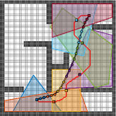
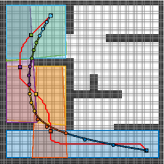
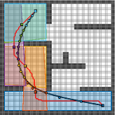
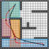
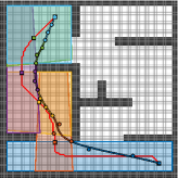
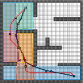
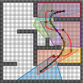
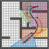
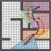
(a)	(b)	(c)	(d)	(e)

Figure 6: Third-order Bézier curve optimization with $C^{1}$ endpoint continuity over convex polygonal safe corridors constructed along a maximal-clearance minimal-length reference path (red): (a) the second-order difference norm, (b) the second-order derivative norm and the first-order difference variance, (c) the first-order difference norm, (d) the first-order derivative norm, (e) the zeroth-order difference variance.

VI Conclusions

In this paper, we introduce a new graph-theoretic approach for designing Bézier curve optimization objectives that measures the alignment of Bézier control points using a quadratic consensus distance derived from the Laplacian of an interaction graph of the control points. We present examples of physical, geometric and statistical consensus distances explicitly constructed using the norms and variances of Bézier curve derivatives and Bézier control-point differences. We demonstrate the use of these quadratic optimization objectives for finding safe and smooth paths over safe corridors. We present an explicit matrix formulation for such constrained quadratic optimization of Bézier curves. We observe that the norm and variance of Bézier continuous derivatives and finite discrete differences of the same order generate similar path profiles. Consequently, owing to the simpler coupling between control points, we conclude that the norm and variance of the finite differences of Bézier control points lead to more intuitive geometric optimization objectives compared to Bézier derivatives. We believe that the unifying graph-theoretic interpretation of Bézier curve optimization opens up new research challenges, including the design of novel interaction graphs for Bézier control points to create new optimization objectives that go beyond Bézier differential norms and variances, for example, for approximately assessing (maximum) curve curvature for curvature-constrained smooth motion planning. Another promising research direction is to perform sensor-based Bézier curve optimization for local planning in dynamic environments [29].

Appendix A Proofs

A-A Proof of Lemma 1

Proof.

The result can be verified using the linearity and cyclic property of the trace operator as

$$\int_{0}^{1}{\mathrm{B}_{\mathbf{P}}(t)}^{\mathrm{T}}\mathrm{B}_{\mathbf{Q}}(t)\mathrm{d}t =\int_{0}^{1}{\mathrm{b}_{n}(t)}^{\mathrm{T}}\mathbf{P}{\mathbf{Q}}^{\mathrm{T}}\mathrm{b}_{m}(t)\mathrm{d}t$$

$$=\int_{0}^{1}\mathrm{tr}\mathopen{}\mathclose{{}\left({\mathbf{Q}}^{\mathrm{T}}\mathrm{b}_{m}(t){\mathrm{b}_{n}(t)}^{\mathrm{T}}\mathbf{P}}\right)\mathrm{d}t$$

$$=\int_{0}^{1}\mathrm{tr}\mathopen{}\mathclose{{}\left({\mathbf{P}}^{\mathrm{T}}\mathrm{b}_{n}(t){\mathrm{b}_{m}(t)}^{\mathrm{T}}\mathbf{Q}}\right)\mathrm{d}t$$

$$=\mathrm{tr}\mathopen{}\mathclose{{}\left({\mathbf{P}}^{\mathrm{T}}\int_{0}^{1}\mathrm{b}_{n}(t){\mathrm{b}_{m}(t)}^{\mathrm{T}}\mathrm{d}t\mathbf{Q}}\right)$$

$$=\mathrm{tr}\mathopen{}\mathclose{{}\left({\mathbf{P}}^{\mathrm{T}}\mathbf{H}_{\mathrm{B}}(n,m)\mathbf{Q}}\right)$$

where each element of $\mathbf{H}_{\mathrm{B}}(n,m)=\int_{0}^{1}\mathrm{b}_{n}(t){\mathrm{b}_{m}(t)}^{\mathrm{T}}\mathrm{d}t$ can be explicitly calculated for $i=0,\ldots n$ and $j=0,\ldots m$ as

$$\mathopen{}\mathclose{{}\left[\mathbf{H}_{\mathrm{B}}(n,m)}\right]_{i+1,j+1} =\int_{0}^{1}\mathrm{b}_{i,n}(t)\mathrm{b}_{j,m}(t)\mathrm{d}t$$

$$=\frac{\binom{n}{i}\binom{m}{j}}{\binom{m+n}{i+j}}\int_{0}^{1}\mathrm{b}_{i+j,m+n}(t)\mathrm{d}t$$

$$=\tfrac{1}{m+n+1}\frac{\binom{n}{i}\binom{m}{j}}{\binom{m+n}{i+j}}$$

which is due to the product and integral properties of Bernstein polynomials, i.e., $\mathrm{b}_{i,n}(t)\mathrm{b}_{j,m}(t)=\frac{\binom{n}{i}\binom{m}{j}}{\binom{m+n}{i+j}}\mathrm{b}_{i+j,m+n}(t)$ and $\int_{0}^{1}\mathrm{b}_{i,n}(t)\mathrm{d}t=\frac{1}{n+1}$ for all $i=0,\ldots,n$ [32]. ∎

A-B Proof of Lemma 2

Proof.

The mean relation simply follows from the constant definite integral property of Bernstein polynomials, i.e., $\int_{0}^{1}b_{i,n}(t)\mathrm{d}t=\frac{1}{n+1}$ [31], as

$$\mu(\mathrm{B}_{\mathbf{P}}) =\int_{0}^{1}\mathrm{B}_{\mathbf{P}}(t)\mathrm{d}t=\int_{0}^{1}\sum_{i=0}^{n}b_{i,n}(t)\mathrm{p}_{i}\mathrm{d}t$$

$$=\sum_{i=0}^{n}\mathrm{p}_{i}\underbrace{\int_{0}^{1}b_{i,n}(t)\mathrm{d}t}_{\frac{1}{n+1}}=\tfrac{1}{n+1}\sum_{i=0}^{n+1}\mathrm{p}_{i}=\mu(\mathbf{P}).$$

The variances of a Bézier curve and its control points can be calculated using the fact that $\mathrm{B}_{\mathbf{P}}(t)-\mu(\mathrm{B}_{\mathbf{P}})=\mathrm{B}_{\mathbf{S}(n)\mathbf{P}}(t)$ and $\mathrm{tr}\mathopen{}\mathclose{{}\left({\mathbf{P}}^{\mathrm{T}}\mathbf{P}}\right)=\sum_{i=0}^{n}\|\mathrm{p}_{i}\|^{2}$ as

$$\sigma^{2}(\mathrm{B}_{\mathbf{P}}) =\int_{0}^{1}\|\mathrm{B}_{\mathbf{P}}(t)-\mu(\mathrm{B}_{\mathbf{P}})\|^{2}\mathrm{d}t=\int_{0}^{1}\|\mathrm{B}_{\mathbf{S}(n)\mathbf{P}}(t)\|^{2}\mathrm{d}t$$

$$=\mathrm{tr}\mathopen{}\mathclose{{}\left({\mathbf{P}}^{\mathrm{T}}\mathbf{S}(n)\mathbf{H}_{\mathrm{N}}(n)\mathbf{S}(n)\mathbf{P}}\right)$$

$$\sigma^{2}(\mathbf{P}) =\tfrac{1}{n+1}\sum_{i=0}^{n}\|\mathrm{p}_{i}-\overline{\mu}(\mathrm{B}_{\mathbf{P}})\|^{2}=\tfrac{1}{n+1}\mathrm{tr}\mathopen{}\mathclose{{}\left({\mathbf{P}}^{\mathrm{T}}\mathbf{S}(n)\mathbf{P}}\right).$$

Hence, $\sigma^{2}(\mathrm{B}_{\mathbf{P}})\leq\frac{1}{n+1}\sigma^{2}(\mathbf{P})$ since we have² $\mathbf{0}\preceq\mathbf{H}_{\mathrm{N}}(n)\preceq\frac{1}{n+1}\mathbf{I}$ and $\mathbf{S}(n)\mathbf{S}(n)=\mathbf{S}(n)$, which completes the proof. ∎

Appendix B Higher-Order Bernstein & Bézier Derivatives

Higher-order derivatives of Bernstein basis polynomials can be calculated explicitly [32, 31].

Lemma 3

(Higher-Order Bernstein Derivatives) The $k^{\text{th}}$-order derivative of the $i^{\text{th}}$ Bernstein basis polynomial $b_{i,n}(t)=\binom{n}{i}t^{i}(1-t)^{n-i}$ of degree $n$ is given by

$$\frac{\mathrm{d}^{k}}{\mathrm{d}t^{k}}b_{i,n}(t)=\frac{n!}{(n-k)!}\sum_{j=0}^{k}\binom{k}{j}(-1)^{k-j}b_{i-j,n-k}(t).$$

Proof.

The results can be verified using the general Leibniz rule, $(fg)^{(k)}=\sum_{j=0}^{k}\binom{k}{j}f^{(j)}g^{(k-j)}$, as

$$\frac{\mathrm{d}^{k}}{\mathrm{d}t^{k}}b_{i,n}(t) \hskip 31.29802pt=\frac{\mathrm{d}^{k}}{\mathrm{d}t^{k}}\tbinom{n}{i}t^{i}(1-t)^{n-i}$$

$$=\tbinom{n}{i}\sum_{j=0}^{k}\tbinom{k}{j}\underbrace{\frac{\mathrm{d}^{j}}{\mathrm{d}t^{j}}t^{i}}_{=\frac{i!}{(i-j)!}t^{i-j}}\overbrace{\frac{\mathrm{d}^{k-j}}{\mathrm{d}t^{k-j}}(1-t)^{n-i}}^{=\frac{(n-i)!}{(n-k-i+j)!}(1\!-\!t)^{n-k-i+j}(-1)^{k-j}}$$

$$=\tbinom{n}{i}\sum_{j=0}^{k}\tbinom{k}{j}\tfrac{i!}{(i-j)!}t^{i-j}\tfrac{(n-i)!}{(n-k-i+j)!}(1-t)^{n-k-i+j}(-1)^{k-j}$$

$$=\sum_{j=0}^{k}\tbinom{n}{i}\tbinom{k}{j}\tfrac{i!}{(i-j)!}\tfrac{(n-i)!}{(n-k-i+j)!}\frac{1}{\binom{n-k}{i-j}}(-1)^{k-j}b_{i-j,n-k}(t)$$

$$=\sum_{j=0}^{k}\tbinom{n}{i}\tbinom{k}{j}\frac{n!}{\binom{n}{i}}\frac{\binom{n-k}{i-j}}{(n-k)!}\frac{1}{\binom{n-k}{i-j}}(-1)^{k-j}b_{i-j,n-k}(t)$$

$$=\tfrac{n!}{(n-k)!}\sum_{j=0}^{k}\tbinom{k}{j}(-1)^{k-j}b_{i-j,n-k}(t)$$

where $\frac{\mathrm{d}^{j}}{\mathrm{d}t^{j}}t^{i}=\frac{i!}{(i-j)!}t^{i-j}$ and $\frac{\mathrm{d}^{j}}{\mathrm{d}t^{j}}(1\!-\!t)^{i}=\frac{i!(-1)^{j}}{(i-j)!}(1\!-\!t)^{i-j}$. ∎

Accordingly, higher-order derivatives of a Bézier curve can be analytically determined as

$$\frac{\mathrm{d}^{k}}{\mathrm{d}t^{k}}\mathrm{B}_{\mathrm{p}_{0},\ldots,\mathrm{p}_{n}}(t) =\sum_{i=0}^{n}\mathrm{p}_{i}\frac{\mathrm{d}^{k}}{\mathrm{d}t^{k}}b_{i,n}(t)$$

$$=\tfrac{n!}{(n-k)!}\sum_{i=0}^{n}\mathrm{p}_{i}\sum_{j=0}^{k}\binom{k}{j}(-1)^{k-j}b_{i-j,n-k}(t)$$

$$=\tfrac{n!}{(n-k)!}\sum_{i=0}^{n-k}\underbrace{\sum_{j=0}^{k}\binom{k}{j}(-1)^{k-j}\mathrm{p}_{i+j}}_{\mathrm{q}_{i}}b_{i,n-k}(t)$$

$$=\tfrac{n!}{(n-k)!}\sum_{i=0}^{n-k}\mathrm{q}_{i}b_{i,n-k}(t)$$

$$=\tfrac{n!}{(n-k)!}\mathrm{B}_{\mathrm{q}_{0},\ldots,\mathrm{q}_{n-k}}(t)$$

where $\mathrm{q}_{i}=\sum_{j=0}^{k}\binom{k}{j}(-1)^{k-j}\mathrm{p}_{i+j}$ for $i=0,\ldots,n-k$.

References

- [1] D. Mellinger and V. Kumar, “Minimum snap trajectory generation and control for quadrotors,” in IEEE International Conference on Robotics and Automation, 2011, pp. 2520–2525.
- [2] C. Richter, A. Bry, and N. Roy, Polynomial Trajectory Planning for Aggressive Quadrotor Flight in Dense Indoor Environments. Springer, 2016, ch. Robotics Research: International Symposium on Robotics Research, pp. 649–666.
- [3] W. Ding, W. Gao, K. Wang, and S. Shen, “An efficient B-spline-based kinodynamic replanning framework for quadrotors,” IEEE Transactions on Robotics, vol. 35, no. 6, pp. 1287–1306, 2019.
- [4] F. Gao, W. Wu, Y. Lin, and S. Shen, “Online safe trajectory generation for quadrotors using fast marching method and Bernstein basis polynomial,” in IEEE Int. Conf. Robot. Autom., 2018, pp. 344–351.
- [5] J. Tordesillas, B. T. Lopez, M. Everett, and J. P. How, “Faster: Fast and safe trajectory planner for navigation in unknown environments,” IEEE Transactions on Robotics, pp. 1–17, 2021.
- [6] D. González, J. Pérez, V. Milanés, and F. Nashashibi, “A review of motion planning techniques for automated vehicles,” IEEE Trans. Intell. Transp. Syst., vol. 17, no. 4, pp. 1135–1145, 2016.
- [7] W. Ding, L. Zhang, J. Chen, and S. Shen, “Safe trajectory generation for complex urban environments using spatio-temporal semantic corridor,” IEEE Robot. Autom. Lett., vol. 4, no. 3, pp. 2997–3004, 2019.
- [8] X. Qian, I. Navarro, A. de La Fortelle, and F. Moutarde, “Motion planning for urban autonomous driving using Bézier curves and MPC,” in IEEE Inter. Conf. Intell. Transp. Syst., 2016, pp. 826–833.
- [9] J. Pérez, J. Godoy, J. Villagrá, and E. Onieva, “Trajectory generator for autonomous vehicles in urban environments,” in IEEE International Conference on Robotics and Automation, 2013, pp. 409–414.
- [10] H. Ozaki and C.-J. Lin, “Optimal B-spline joint trajectory generation for collision-free movements of a manipulator under dynamic constraints,” in IEEE Int. Conf. Robot. Autom., 1996, pp. 3592–3597.
- [11] K. Hauser and V. Ng-Thow-Hing, “Fast smoothing of manipulator trajectories using optimal bounded-acceleration shortcuts,” in IEEE Int. Conf. Robot. Autom., 2010, pp. 2493–2498.
- [12] C. Scheiderer, T. Thun, and T. Meisen, “Bézier curve based continuous and smooth motion planning for self-learning industrial robots,” Procedia Manufacturing, vol. 38, pp. 423–430, 2019.
- [13] X. Zhao, Z. Cao, W. Geng, Y. Yu, M. Tan, and X. Chen, “Path planning of manipulator based on RRT-connect and Bézier curve,” in IEEE International Conference on CYBER Technology in Automation, Control, and Intelligent Systems, 2019, pp. 649–653.
- [14] A. Bry, C. Richter, A. Bachrach, and N. Roy, “Aggressive flight of fixed-wing and quadrotor aircraft in dense indoor environments,” Int. J. Robot. Res., vol. 34, no. 7, pp. 969–1002, 2015.
- [15] F. Gao, W. Wu, W. Gao, and S. Shen, “Flying on point clouds: Online trajectory generation and autonomous navigation for quadrotors in cluttered environments,” Journal of Field Robotics, vol. 36, pp. 710–733, 2019.
- [16] M. J. Van Nieuwstadt and R. M. Murray, “Real-time trajectory generation for differentially flat systems,” International Journal of Robust and Nonlinear Control, vol. 8, no. 11, pp. 995–1020, 1998.
- [17] J. Chen, K. Su, and S. Shen, “Real-time safe trajectory generation for quadrotor flight in cluttered environments,” in IEEE International Conference on Robotics and Biomimetics, 2015, pp. 1678–1685.
- [18] S. Liu, M. Watterson, K. Mohta, K. Sun, S. Bhattacharya, C. J. Taylor, and V. Kumar, “Planning dynamically feasible trajectories for quadrotors using safe flight corridors in 3-d complex environments,” IEEE Robotics and Automation Letters, vol. 2, no. 3, pp. 1688–1695, 2017.
- [19] J. Chen, T. Liu, and S. Shen, “Online generation of collision-free trajectories for quadrotor flight in unknown cluttered environments,” in IEEE International Conference on Robotics and Automation, 2016, pp. 1476–1483.
- [20] S. Quinlan and O. Khatib, “Elastic bands: connecting path planning and control,” in IEEE International Conference on Robotics and Automation, 1993, pp. 802–807.
- [21] Z. Zhu, E. Schmerling, and M. Pavone, “A convex optimization approach to smooth trajectories for motion planning with car-like robots,” in IEEE Conference on Decision and Control, 2015, pp. 835–842.
- [22] B. Zhou, F. Gao, L. Wang, C. Liu, and S. Shen, “Robust and efficient quadrotor trajectory generation for fast autonomous flight,” IEEE Robotics and Automation Letters, vol. 4, no. 4, pp. 3529–3536, Oct 2019.
- [23] W. Hönig, J. A. Preiss, T. K. S. Kumar, G. S. Sukhatme, and N. Ayanian, “Trajectory planning for quadrotor swarms,” IEEE Transactions on Robotics, vol. 34, no. 4, pp. 856–869, 2018.
- [24] J.-w. Choi, R. E. Curry, and G. H. Elkaim, “Continuous curvature path generation based on Bézier curves for autonomous vehicles,” IAENG Int. Journal of Applied Mathematics, vol. 40, no. 2, pp. 91–101, 2010.
- [25] R. Deits and R. Tedrake, “Efficient mixed-integer planning for uavs in cluttered environments,” in IEEE International Conference on Robotics and Automation, 2015, pp. 42–49.
- [26] F. Gao and S. Shen, “Online quadrotor trajectory generation and autonomous navigation on point clouds,” in IEEE International Symposium on Safety, Security, and Rescue Robotics, 2016, pp. 139–146.
- [27] Z. Wang, F. Zou, Z. Ma, T. Liu, and Y. Niu, “Flight corridor construction method for fixed-wing uav obstacle avoidance,” in International Conference on Autonomous Unmanned Systems, 2022, pp. 1808–1818.
- [28] Y. Lin, F. Gao, T. Qin, W. Gao, T. Liu, W. Wu, Z. Yang, and S. Shen, “Autonomous aerial navigation using monocular visual-inertial fusion,” Journal of Field Robotics, vol. 35, no. 1, pp. 23–51, 2018.
- [29] O. Arslan and D. E. Koditschek, “Sensor-based reactive navigation in unknown convex sphere worlds,” The International Journal of Robotics Research, vol. 38, no. 2-3, pp. 196–223, 2019.
- [30] O. Arslan, V. Pacelli, and D. E. Koditschek, “Sensory steering for sampling-based motion planning,” in IEEE/RSJ International Conference on Intelligent Robots and Systems, 2017, pp. 3708–3715.
- [31] R. T. Farouki, “The Bernstein polynomial basis: A centennial retrospective,” Comp. Aided Geom. Design, vol. 29, no. 6, pp. 379–419, 2012.
- [32] G. E. Farin, Curves and surfaces for CAGD: A practical guide. Morgan Kaufmann, 2002.
- [33] O. Arslan and A. Tiemessen, “Adaptive Bézier degree reduction and splitting for computationally efficient motion planning,” IEEE Transactions on Robotics, vol. 38, no. 6, pp. 3655–3674, 2022.
- [34] R. Olfati-Saber, J. A. Fax, and R. M. Murray, “Consensus and cooperation in networked multi-agent systems,” Proceedings of the IEEE, vol. 95, no. 1, pp. 215–233, 2007.
- [35] O. Arslan, “Clustering-based robot navigation and control,” Ph.D. dissertation, University of Pennsylvania, 2016.