abc

Multivariate Singular Spectrum Analysis
by Robust Diagonalwise Low-Rank Approximation
Fabio Centofanti, Mia Hubert, Biagio Palumbo¹, and Peter J. Rousseeuw²
September 30, 2023

Abstract

Multivariate Singular Spectrum Analysis (MSSA) is a powerful and widely used nonparametric method for multivariate time series, which allows the analysis of complex temporal data from diverse fields such as finance, healthcare, ecology, and engineering. However, MSSA lacks robustness against outliers because it relies on the singular value decomposition, which is very sensitive to the presence of anomalous values. MSSA can then give biased results and lead to erroneous conclusions. In this paper a new MSSA method is proposed, named RObust Diagonalwise Estimation of SSA (RODESSA), which is robust against the presence of cellwise and casewise outliers. In particular, the decomposition step of MSSA is replaced by a new robust low-rank approximation of the trajectory matrix that takes its special structure into account. A fast algorithm is constructed, and it is proved that each iteration step decreases the objective function. In order to visualize different types of outliers, a new graphical display is introduced, called an enhanced time series plot. An extensive Monte Carlo simulation study is performed to compare RODESSA with competing approaches in the literature. A real data example about temperature analysis in passenger railway vehicles demonstrates the practical utility of the proposed approach.

Keywords: Casewise outliers; Cellwise outliers; Iteratively reweighted least squares;Multivariate time series; Robust statistics.

1 Introduction

Time series analysis plays a crucial role in understanding and predicting the behavior of sequential data across a wide range of disciplines. It has proven to be an invaluable tool in fields such as finance, healthcare, ecology, engineering, and more. Singular spectrum analysis (SSA) has emerged as a powerful nonparametric tool for extracting valuable insights from time-dependent data. A comprehensive overview of SSA can be found in the books Golyandina et al. (2001), Golyandina and Zhigljavsky (2013), and Golyandina et al. (2018). Numerous examples showcasing the success of SSA can be found in the literature. Multivariate singular spectrum analysis, referred to as MSSA (Broomhead and King, 1986), enables the simultaneous analysis and interpretation of multiple time series, by exploiting the dependencies between variables.

A crucial step of SSA is the low-rank approximation of the so-called trajectory matrix, which will be described in the next section. The most often used tool for this is the singular value decomposition (SVD), which is however sensitive to the presence of outliers in the data. Several authors have proposed outlier-robust SSA methods by replacing the SVD by more robust versions. However, none of these low-rank approximations took the special diagonal structure of the trajectory matrix into account. The main contribution of our work is a new robust low-rank approximation method tailored to this situation.

The paper is organized as follows. Section 2 briefly surveys existing work and introduces the new approach, called RObust Diagonalwise Estimation of SSA (RODESSA), including its algorithm, implementation, and forecasting method. It is proved that each step of the algorithm reduces the objective function. Section 3 proposes an enhanced time series plot in which two types of outliers are represented by colors, in order to assist with outlier detection. In Section 4, the performance of RODESSA is assessed by an extensive Monte Carlo simulation study. Section 5 presents a real data example regarding temperature analysis in passenger railway vehicles. Section 6 concludes the paper.

2 Multivariate singular spectrum analysis

2.1 Classical multivariate SSA

Consider a $p$-variate time series $\mathbb{X}=\left(\mathbb{X}^{(1)},\ldots,\mathbb{X}^{(p)}\right)$, i.e., a collection $\{\mathbb{X}^{(j)}=(x_{i}^{(j)})_{i=1}^{N}\,,$ $j=1,\ldots,p\}$ of $p$ time series of length $N$. Multivariate SSA then proceeds by the following four successive steps.

1. Embedding. In the embedding step, the multivariate time series $\mathbb{X}$ is mapped into a big trajectory matrix $\bm{X}$. Let $L$ be an integer called window length, $1<L<N$. For each time series $\mathbb{X}^{(j)}$ we then form $K_{u}=N-L+1$ lagged vectors $X_{i}^{(j)}=\left(x_{i}^{(j)},\ldots,x_{i+L-1}^{(j)}\right)^{T}$ for $1\leqslant i\leqslant K_{u}$. The trajectory matrix of the multivariate series $\mathbb{X}$ is a matrix of size $L\times K$ with $K=pK_{u}$ , and has the form

$$\mathcal{T}_{\text{MSSA}}(\mathbb{X})=\bm{X} =\left[X_{1}^{(1)}:\ldots:X_{K_{u}}^{(1)}:\ldots:X_{1}^{(p)}:\ldots:X_{K_{u}}^{(p)}\right]=\left[\bm{X}^{(1)}:\ldots:\bm{X}^{(p)}\right]$$ (1)

$$=\left[\begin{matrix}x_{1}^{(1)}&x_{2}^{(1)}&x_{3}^{(1)}&\ldots\\ x_{2}^{(1)}&x_{3}^{(1)}&x_{4}^{(1)}&\ldots\\ x_{3}^{(1)}&x_{4}^{(1)}&x_{5}^{(1)}&\ldots\\ \vdots&\vdots&\vdots&\ddots\\ \end{matrix}\hskip 8.5359pt\vline\hskip 8.5359pt\begin{matrix}x_{1}^{(2)}&x_{2}^{(2)}&x_{3}^{(2)}&\ldots\\ x_{2}^{(2)}&x_{3}^{(2)}&x_{4}^{(2)}&\ldots\\ x_{3}^{(2)}&x_{4}^{(2)}&x_{5}^{(2)}&\ldots\\ \vdots&\vdots&\vdots&\ddots\\ \end{matrix}\hskip 8.5359pt\vline\hskip 8.5359pt\begin{matrix}x_{1}^{(3)}&x_{2}^{(3)}&x_{3}^{(3)}&\ldots\\ x_{2}^{(3)}&x_{3}^{(3)}&x_{4}^{(3)}&\ldots\\ x_{3}^{(3)}&x_{4}^{(3)}&x_{5}^{(3)}&\ldots\\ \vdots&\vdots&\vdots&\ddots\\ \end{matrix}\hskip 8.5359pt\vline\hskip 8.5359pt\begin{matrix}\ldots\\ \ldots\\ \ldots\\ \vdots\\ \end{matrix}\right]$$

where $\bm{X}^{(j)}=\mathcal{T}_{\text{SSA}}\left(\mathbb{X}^{(j)}\right)=\left[X_{1}^{(j)}:\ldots:X_{K_{u}}^{(j)}\right]$ is the trajectory matrix of the one-dimensional series $\mathbb{X}^{(j)}$. Note the (anti-)diagonal structure of each $\bm{X}^{(j)}$, making it a so-called Hankel matrix. The entire matrix $\bm{X}$ is thus a stacked Hankel matrix. The notations $\mathcal{T}_{\text{SSA }}$ and $\mathcal{T}_{\text{MSSA }}$ stand for the univariate and multivariate embedding operators that map $\mathbb{X}^{(j)}$ and $\mathbb{X}$ to the corresponding trajectory matrices.

2. Decomposition. This step performs the SVD of the trajectory matrix $\bm{X}$, yielding

$$\bm{X}=\sum_{r=1}^{d}\beta_{r}\bm{u}_{r}\bm{v}_{r}^{T}$$ (2)

where $d=\operatorname{rank}(\bm{X})$, and $\bm{u}_{1},\ldots,\bm{u}_{d}$ and $\bm{v}_{1},\ldots,\bm{v}_{d}$ are the left and right singular vectors. The ordered singular values are $\beta_{1}\geqslant\cdots\geqslant\beta_{d}>0$, and the matrices $\bm{X}_{r}=\beta_{r}\bm{u}_{r}\bm{v}_{r}^{T}$ all have rank 1. The triple $\left(\beta_{r},\bm{u}_{r},\bm{v}_{r}\right)$ is called the $r$-th eigentriple of the matrix $\bm{X}$.

3. Grouping. The grouping step corresponds to splitting the terms of (2) into several disjoint groups and summing the matrices within each group. In this paper we focus on the case where two main groups are created, and we write

$$\bm{X}=\bm{\widehat{X}}_{q}+\bm{R}$$ (3)

where the estimate of the signal $\bm{\widehat{X}}_{q}$ is a sum like (2) but only for the first $q$ eigentriples, whereas the residual matrix $\bm{R}=\bm{X}-\bm{\widehat{X}}_{q}$ is associated with the noise. We can see $\bm{\widehat{X}}_{q}$ as a low-rank approximation of the trajectory matrix.

4. Reconstruction. In this step, the fitted matrix $\bm{\widehat{X}}_{q}$ is transformed back to the form of the input object $\mathbb{X}$ in (1). In each submatrix $\bm{\widehat{X}}_{q}^{(j)}$ we compute average entries as follows. Denote an anti-diagonal as $A_{i}=\{(l,k):l+k=i+1,1\leqslant l\leqslant L,1\leqslant k\leqslant K_{u}\}$ with its cardinality $n_{i}=|A_{i}|$. Each matrix $\bm{\widehat{X}}_{q}^{(j)}=(\widehat{X}_{lk}^{(j)})_{lk}$ is turned into a new series $\widehat{\mathbb{X}}^{(j)}=(\hat{x_{i}}^{(j)})_{i=1,\ldots,N}$ of length $N$, with

$$\hat{x}_{i}^{(j)}:=\frac{1}{n_{i}}\sum_{(l,k)\in A_{i}}\widehat{X}^{(j)}_{lk}\;.$$ (4)

The reconstructed multivariate time series is then given by $\widehat{\mathbb{X}}=\left(\widehat{\mathbb{X}}^{(1)},\ldots,\widehat{\mathbb{X}}^{(p)}\right)$.

2.2 Outliers in multivariate time series

Multivariate time series may contain outliers, that is, observations that deviate from the expected patterns or trends. They can be caused by a variety of factors such as measurement errors, data entry mistakes, sensor malfunctions, or rare and unexpected events. Outliers can bias statistical measures, affect parameter estimation, and lead to inaccurate forecasting, resulting in erroneous conclusions and flawed decision-making. As in the multivariate setting (Alqallaf et al., 2009; Raymaekers and Rousseeuw, 2023), we distinguish between a cellwise outlier, which is an outlying value $x_{i}^{(j)}$ in the $j$-th univariate time series only, and a casewise outlier, where at a time $i$ several or all of the values $x_{i}^{(j)}$ deviate simultaneously.

Figure 1 illustrates this for a 3-variate time series. The purple triangle is a cellwise outlier which affects only the first univariate time series at time $i=3$, whereas the orange squares indicate a casewise outlier at time point $i=5$. The effect of both types of outliers on the trajectory matrix (1) is shown in the bottom part of the figure. The cellwise outlier corresponds to an antidiagonal in the leftmost Hankel matrix only, whereas the casewise outlier affects all three stacked Hankel matrices.

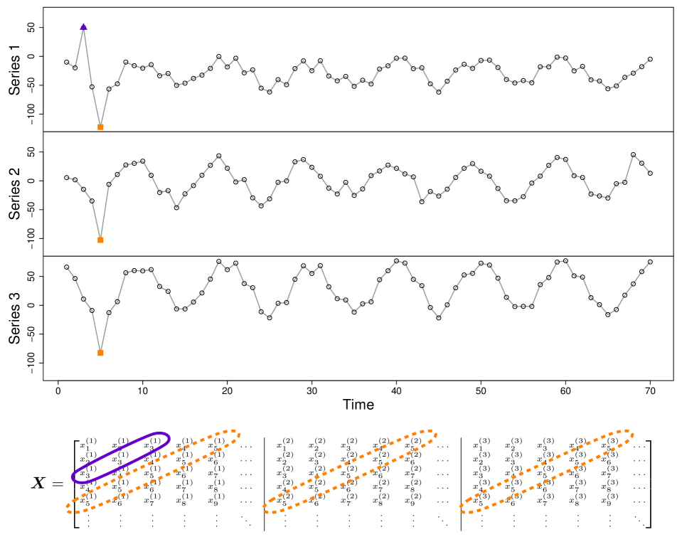
Figure 1: The effect of a cellwise outlier (purple triangle) and a casewise outlier (orange squares) on the diagonals of the trajectory matrix $\bm{X}$.

2.3 Existing robust SSA methods

Classical MSSA, and its univariate version SSA, are sensitive to outliers because they are based on the SVD which is highly susceptible to outlying values. In order to remedy this, there has been research into the construction of outlier-robust SSA methods. In general, the purpose of robust methods is to limit the effect of outliers on the results, after which the outliers can be detected by their residuals from the robust fit, see e.g. Rousseeuw and Leroy (1987), Maronna et al. (2019).

When constructing a more robust version of SSA one needs to replace the classical SVD by something less sensitive to outliers. One approach is to start from an outlier-robust principal component analysis (PCA) method. A PCA fit of rank $q$ is of the type

$$\bm{\widehat{X}}=\bm{1}_{n}\bm{\hat{\mu}}^{T}+\bm{U}\bm{V}^{T}$$ (5)

where $\bm{\hat{\mu}}$ is the estimated center, and the matrix of scores $\bm{U}$ as well as the loadings matrix $\bm{V}$ have $q$ columns. Many PCA methods have an option to set $\bm{\hat{\mu}}=\mathbf{0}$, and then (5) yields an approximation of rank $q$ to $\bm{X}$ as in (3). Afterward one can carry out the reconstruction step of SSA. De Klerk (2015) applied the robust PCA method ROBPCA (Hubert et al., 2005) to the trajectory matrix, and then centered the original data $\bm{X}$ as well as $\bm{\widehat{X}}$ by subtracting $\bm{1}_{n}\bm{\hat{\mu}}^{T}$. In this way he obtained a robust centered SSA method.

A limitation of this approach is that ROBPCA and most other robust PCA methods are built to withstand outlying rows of the data matrix, but not outlying cells. But we have seen in the bottom part of Figure 1 that a single outlying value in a time series can affect many cells of the trajectory matrix $\bm{X}$, especially when the window length $L$ is high. Therefore a relatively small number of outliers in the time series can affect over half the rows of $\bm{X}$, which ROBPCA might not withstand. In such situations a cellwise robust PCA method like MacroPCA (Hubert et al., 2019) could be used instead.

In the nonrobust setting, expression (3) can equivalently be seen as a problem of low-rank approximation of the trajectory matrix $\bm{X}$ by a matrix $\widehat{\bm{X}}_{L^{2}}$ , which minimizes

$$||\bm{X}-\bm{S}||^{2}_{F}$$

over all $L\times K$ matrices $\bm{S}$ of rank $q$. Writing the unknown $\bm{S}$ as a product $\bm{S}=\bm{U}\bm{V}^{T}$, where $\bm{U}=\left[\bm{u}_{1},\dots,\bm{u}_{q}\right]=\left(\left[\bm{u}^{1},\dots,\bm{u}^{L}\right]\right)^{T}$ is $L\times q$ with $\bm{u}_{i}=\left(u_{i1},\dots,u_{iL}\right)^{T}$, and $\bm{V}=\left[\bm{v}_{1},\dots,\bm{v}_{q}\right]=\left(\left[\bm{v}^{1},\dots,\bm{v}^{K}\right]\right)^{T}$ is $K\times q$ with $\bm{v}_{i}=\left(v_{i1},\dots,v_{iK}\right)^{T}$, this is equivalent to minimizing

$$||\bm{X}-\bm{U}\bm{V}^{T}||^{2}_{F}=\sum_{\ell=1}^{L}\sum_{k=1}^{K}\left(X_{\ell k}-\sum_{r=1}^{q}u_{\ell r}v_{kr}\right)^{2}=\sum_{\ell=1}^{L}\sum_{k=1}^{K}R_{\ell k}^{2}$$ (6)

with the residuals $R_{\ell k}:=X_{\ell k}-\sum_{r=1}^{q}u_{\ell r}v_{kr}$ . We then put $\widehat{\bm{X}}_{L^{2}}:=\widehat{\bm{U}}_{L^{2}}\widehat{\bm{V}}_{L^{2}}^{T}$. The solution of the optimization (6) is easily obtained through the SVD decomposition $\bm{X}=\bm{\widetilde{U}}\bm{D}\bm{\widetilde{V}}^{T}$ where $\bm{D}$ is the diagonal matrix of singular values. Restricting this to the $q$ leading singular values $\beta_{1}\geqslant\ldots\geqslant\beta_{q}>0$ we obtain $\bm{\widehat{X}}=\bm{\widetilde{U}}_{q}\bm{D}_{q}\bm{\widetilde{V}}_{q}^{T}$. We can then absorb the singular values by putting $\widehat{\bm{U}}_{L^{2}}=\bm{\widetilde{U}}_{q}\bm{D}_{q}^{1/2}$ and $\widehat{\bm{V}}_{L^{2}}=\bm{\widetilde{V}}_{q}\bm{D}_{q}^{1/2}$, so that indeed $\widehat{\bm{X}}=\widehat{\bm{U}}_{L^{2}}\widehat{\bm{V}}_{L^{2}}^{T}$ . But the quadratic loss function in (6) makes this a least squares fit, which is very sensitive to outliers.

To remedy this, De la Torre and Black (2003) proposed a more robust low-rank approximation by replacing (6) by the minimization of the loss function

$$L_{\rho}\left(\bm{X}-\bm{U}\bm{V}^{T}\right):=\sum_{\ell=1}^{L}\sum_{k=1}^{K}\rho\left(\frac{X_{\ell k}-\sum_{r=1}^{q}u_{\ell r}v_{kr}}{\hat{\sigma}}\right)=\sum_{\ell=1}^{L}\sum_{k=1}^{K}\rho\left(\frac{R_{\ell k}}{\hat{\sigma}}\right),$$ (7)

where $\hat{\sigma}$ is a fixed scale estimate. The function $\rho$ must be continuous, even, non-decreasing for positive arguments, and satisfy $\rho(0)=0$. De la Torre and Black (2003) used

$$\rho(t)=\frac{t^{2}}{t^{2}+1}$$

that goes to 1 as $t\rightarrow\infty$. Therefore an outlying $t$ has much less effect on $\rho(t)$ than with the $\rho(t)=t^{2}$ in (6). They constructed an iterative algorithm for $\bm{\widehat{U}}\bm{\widehat{V}}^{T}$. For $\hat{\sigma}$ they took the median absolute deviation of the residuals from an initial estimate $\bm{U}_{0}\bm{V}_{0}^{T}$.

Note that here and in the sequel the estimation target is not the pair $(\bm{U},\bm{V})$ because that is not uniquely defined. Indeed, if we take a nonsingular $q\times q$ matrix $\bm{A}$ we see that $(\bm{U}\bm{A},\bm{V}(\bm{A}^{-1})^{T})$ yields the same product $\bm{U}\bm{A}\bm{A}^{-1}\bm{V}^{T}=\bm{U}\bm{V}^{T}$ as $(\bm{U},\bm{V})$, and hence the same objective (7). The actual estimation target is the product $\bm{U}\bm{V}^{T}$ .

Chen and Sacchi (2015) applied this general low-rank approximation method to the decomposition step of SSA. They replaced the function $\rho$ by Tukey’s biweight function

$$\rho_{c}(t)=\begin{cases}\displaystyle 1-\left(1-\frac{t^{2}}{c^{2}}\right)^{3}&|t|\leqslant c\\ 1&|t|>c\end{cases}$$ (8)

with tuning constant $c=4.685$, and used the method to filter seismic noise.

Rodrigues et al. (2018) also constructed a robust SSA from the low-rank approximation method of De la Torre and Black (2003), but replaced the function $\rho$ by $\rho(t)=|t|$ as in Croux et al. (2003), yielding an $L^{1}$ objective. An advantage of the latter $\rho$ function is that $\hat{\sigma}$ can be moved out of (7), so one does not need to estimate $\sigma$ in advance. In subsequent work, Rodrigues et al. (2020) carried out robust SSA based on the low-rank approximation of Zhang et al. (2013) which used the Huber function

$$\rho_{b}(t)=\frac{t^{2}}{2}I(|t|\leqslant b)+\left(b|t|-\frac{b^{2}}{2}\right)I(|t|>b)$$ (9)

with $b=1.345$. Cheng et al. (2015) performed a robust SSA analysis by applying a different robust low-rank approximation method due to Candès et al. (2011).

2.4 The RODESSA objective function

The existing robust low-rank approximation methods described above are less sensitive to outliers than the classical SVD. But none of them are tailored to the (possibly stacked) Hankel structure of the trajectory matrix $\bm{X}$. As we saw in the bottom part of Figure 1, an outlier in one of the time series corresponds to an entire diagonal of the corresponding trajectory matrix. In the least squares low-rank approximation setting, algorithms have been developed that incorporate the Hankel structure of $\bm{X}$ (Markovsky, 2008), but no such approach exists in the robust setting yet.

To fill this gap we propose a new robust method for MSSA, named RObust Diagonalwise Estimation of SSA (RODESSA), which explicitly takes into account the way outliers and their residuals occur in the stacked Hankel structure of the trajectory matrix. It is meaningful to talk about anomalous diagonals rather than anomalous rows of the trajectory matrix $\bm{X}$. Therefore we propose to approximate the trajectory matrix $\bm{X}$ by $\widehat{\bm{X}}=\bm{U}\bm{V}^{T}$ obtained by minimizing

$$L_{\rho_{1},\rho_{2}}\left(\bm{X}-\bm{U}\bm{V}^{T}\right):=\sum_{i=1}^{N}pn_{i}\hat{\sigma}_{2}^{2}\rho_{2}\left(\frac{\sum_{j=1}^{p}n_{i}\hat{\sigma}_{1,j}^{2}\rho_{1}\left(\sum_{a=1}^{n_{i}}(x_{i}^{(j)}-\hat{x}_{ia}^{(j)})^{2}/(n_{i}\hat{\sigma}_{1,j}^{2})\right)}{pn_{i}\hat{\sigma}_{2}^{2}}\right)$$ (10)

over $(\bm{U},\bm{V})$ with $\operatorname{rank}(\bm{U}\bm{V}^{T})=q$. Here $p$ is again the number of univariate time series and $n_{i}$ is the length of the diagonal corresponding to $x_{i}^{(j)}$ as in (4). The predicted cell $\hat{x}_{ia}^{(j)}$ is given by $\sum_{r=1}^{q}u_{i^{*}r}v_{a^{*}r}$ with $i^{*}=\min\{L,i\}+1-a$ and $a^{*}=\min\{K_{u},i\}-(n_{i}-a)+K_{u}(j-1)$. The fixed scales $\hat{\sigma}_{1,j}^{2}$ standardize the squared norms of the diagonal residuals of series $j$, given by

$$r_{i}^{(j)}:=\frac{1}{n_{i}}\sum_{a=1}^{n_{i}}(x_{i}^{(j)}-\hat{x}_{ia}^{(j)})^{2}\;.$$ (11)

The overall scale $\hat{\sigma}_{2}^{2}$ standardizes the quantities

$$r_{i}:=\frac{1}{p}\sum_{j=1}^{p}\hat{\sigma}_{1,j}^{2}\rho_{1}\left(\frac{r_{i}^{(j)}}{\hat{\sigma}_{1,j}^{2}}\right)$$ (12)

based on all $p$ coordinates. The functions $\rho_{1}$ and $\rho_{2}$ are defined for nonnegative arguments and must be continuous and non-decreasing. In our implementation both are of the form $\rho(t):=\rho_{c}(\sqrt{t})$ where $\rho_{c}$ is Tukey’s biweight (8). [For $\rho_{1}(t)=\rho_{2}(t)=|t|$, (10) would reduce to (6).] The goal of the normalization by $n_{i}\hat{\sigma}_{1j}^{2}$ inside $\rho_{1}$ in (10) is to give the $r_{i}^{(j)}$ similar average sizes. Indeed, if the $x_{i}^{(j)}-\hat{x}_{ia}^{(j)}$ would be independent normal random variables with variance $\hat{\sigma}_{1j}^{2}$ , then $n_{i}r_{i}^{(j)}$ would follow a Gamma distribution with parameters $n_{i}/2$ and $2\hat{\sigma}_{1j}^{2}$ and thus with mean equal to $n_{i}\hat{\sigma}_{1j}^{2}$ . Therefore the average of the $r_{i}^{(j)}/\hat{\sigma}_{1j}^{2}$ would be close to 1. A similar argument applies for the normalization by $pn_{i}\hat{\sigma}_{2}^{2}$ inside $\rho_{2}$ .

The functions $\rho_{1}$ and $\rho_{2}$ reduce the effect of cellwise and casewise outliers on the final estimates, because large values of $r_{i}^{(j)}$ and/or $r_{i}$ contribute less to the objective function. We can say that $r_{i}^{(j)}$ measures how prone the $i$-th value $x_{i}^{(j)}$ of time series $j$ is to be a cellwise outlier. Analogously, $r_{i}$ reflects how prone the multivariate $\bm{x}_{i}=(x_{i}^{(1)},\ldots,x_{i}^{(p)})^{T}$ is to be a casewise outlier. Note that in the computation of $r_{i}$ the effect of cellwise outliers is tempered by the presence of $\rho_{1}$ , to avoid that a single cellwise outlier would always result in a large casewise $r_{i}$ .

2.5 The IRLS algorithm

We now address the optimization problem (10). The scale estimates $\hat{\sigma}_{1,j}$ and $\hat{\sigma}_{2}$ are constants, whose computation will be described in Section 2.6. Because $L_{\rho_{1},\rho_{2}}$ is continuously differentiable, its solution must satisfy the first-order necessary conditions for optimality. They are obtained by setting the gradients of $L_{\rho_{1},\rho_{2}}$ with respect to $\bm{u}^{1},\dots,\bm{u}^{L}$ and $\bm{v}^{1},\dots,\bm{v}^{K}$ to zero, yielding

$$\bm{V}^{T}\bm{W}^{\ell}(\bm{V}\bm{u}^{\ell}-\bm{X}^{\ell}) =\bm{0},\quad\ell=1,\dots,L,$$

$$\bm{U}^{T}\bm{W}_{k}(\bm{U}\bm{v}^{k}-\bm{X}_{k}) =\bm{0},\quad k=1,\dots,K,$$ (13)

where $\bm{X}^{1},\dots,\bm{X}^{L}$ and $\bm{X}_{1},\dots,\bm{X}_{K}$ are the rows and columns of $\bm{X}$. Here $\bm{W}^{\ell}$ is a $K\times K$ diagonal matrix, whose diagonal entries are equal to the $\ell$th row of the $L\times K$ weight matrix

$$\bm{W}=\{w_{\ell k}\}=\bm{\widetilde{W}}_{c}\odot\bm{\widetilde{W}}_{r}$$ (14)

where the Hadamard product $\odot$ multiplies matrices entry by entry. Analogously, $\bm{W}_{k}$ is an $L\times L$ diagonal matrix, whose diagonal entries are the $k$th column of the matrix $\bm{W}$. The matrix $\bm{\widetilde{W}}_{c}$ in (14) is given by $\bm{\widetilde{W}}_{c}=\left[\bm{\widetilde{W}}_{c}^{(1)}:\ldots:\bm{\widetilde{W}}_{c}^{(p)}\right]$ with $\bm{\widetilde{W}}_{c}^{(j)}=\mathcal{T}_{\mathrm{SSA}}\left(w_{c,1}^{(j)},\dots,w_{c,N}^{(j)}\right)$, containing the cellwise weights

$$w_{c,i}^{(j)}=\rho_{1}^{\prime}\left(r_{i}^{(j)}/\hat{\sigma}^{2}_{1j}\right),\quad i=1,\dots,N,\quad j=1\dots,p,$$ (15)

in which $\rho_{1}^{\prime}$ is the derivative of $\rho_{1}$ . The matrix $\bm{\widetilde{W}}_{r}$ is given by $\bm{\widetilde{W}}_{r}=\left[\bm{\widetilde{W}}_{r}^{(1)}:\ldots:\bm{\widetilde{W}}_{r}^{(p)}\right]$, with each $\bm{\widetilde{W}}_{r}^{(j)}=\mathcal{T}_{\mathrm{SSA}}\left(w_{r,1},\dots,w_{r,N}\right)$ containing the same casewise weights

$$w_{r,i}=\rho_{2}^{\prime}\left(r_{i}/\hat{\sigma}^{2}_{2}\right),\quad i=1,\dots,N\,.$$ (16)

Outlying cells $x_{i}^{(j)}$ should get a small cellwise weight $w_{c,i}^{(j)}$  and outlying cases $\bm{x}_{i}$ should get a small casewise weight $w_{r,i}$ .

The system (2.5) is nonlinear because the weight matrices depend on the estimate, and the estimate depends on the weight matrices. In such a situation one can resort to an iteratively reweighted least squares (IRLS) algorithm. Note that for a fixed weight matrix $\bm{W}$, the system (2.5) coincides with the first-order necessary condition of the weighted least squares problem of minimizing

$$\sum_{\ell=1}^{L}\sum_{k=1}^{K}w_{\ell k}\left(X_{\ell k}-\widehat{X}_{\ell k}\right)^{2}$$ (17)

where $\widehat{X}_{\ell k}=\sum_{r=1}^{q}u_{\ell r}v_{kr}$. The optimization of (17) can be performed by alternating least squares (Gabriel, 1978). This minimizes (17) with respect to $\bm{u}^{1},\dots,\bm{u}^{L}$ where $\bm{v}^{1},\dots,\bm{v}^{K}$ and the weights are fixed, and alternates this with minimizing (17) with respect to $\bm{v}^{1},\dots,\bm{v}^{K}$ where $\bm{u}^{1},\dots,\bm{u}^{L}$ and the weights are fixed.

The overall algorithm starts from initial estimates $\bm{U}_{0},\bm{V}_{0}$ of $\bm{U},\bm{V}$ that will be described in Section 2.6. New matrices $\bm{U}_{t+1}$, $\bm{V}_{t+1}$ are obtained from $\bm{U}_{t}$, $\bm{V}_{t}$ by

$$\bm{v}^{k}_{t+1}=\left(\bm{U}_{t}^{T}\bm{W}_{k,t}\bm{U}_{t}\right)^{-1}\bm{U}_{t}^{T}\bm{W}_{k,t}\bm{X}_{k}\quad \mbox{for}\quad k=1,\dots,K,$$

$$\bm{u}_{t+1}^{\ell}=\left(\bm{V}_{t+1}^{T}\bm{W}_{t}^{\ell}\bm{V}_{t+1}\right)^{-1}\bm{V}_{t+1}^{T}\bm{W}^{\ell}_{t}\bm{X}^{\ell}\quad \mbox{for}\quad\ell=1,\dots,L.$$ (18)

Then the weight matrix is updated to $\bm{W}_{t+1}$ as in (14). The iterative process continues until convergence, as summarized in Algorithm 1.

Algorithm 1 IRLS algorithm

1:Compute $\bm{U}_{0},\bm{V}_{0}$, $\hat{\sigma}_{1,j}$ and $\hat{\sigma}_{2}$ according to Section 2.6 $\blacktriangleright$ Initialization

2:Set $t=0$

3:Compute $\bm{W}_{0}$ as in (14)

4:repeat

5:   $\bm{v}^{k}_{t+1}=\left(\bm{U}_{t}^{T}\bm{W}_{k,t}\bm{U}_{t}\right)^{-1}\bm{U}_{t}^{T}\bm{W}_{k,t}\bm{X}_{k}\quad\mbox{for}\quad k=1,\dots,K$

6:   $\bm{u}_{t+1}^{\ell}=\left(\bm{V}_{t+1}^{T}\bm{W}_{t}^{\ell}\bm{V}_{t+1}\right)^{-1}\bm{V}_{t+1}^{T}\bm{W}^{\ell}_{t}\bm{X}^{\ell}\quad\mbox{for}\quad\ell=1,\dots,L$

7:   Compute $\bm{W}_{t+1}$ as in (14) $\blacktriangleright$ Weight matrix update

8:   $t=t+1$

9:until $\;||\bm{U}_{t}\bm{V}_{t}^{T}-\bm{U}_{t-1}\bm{V}_{t-1}^{T}||_{F}<\nu\,||\bm{U}_{t-1}\bm{V}_{t-1}^{T}||_{F}$  for some tolerance $\nu$.

Proposition 1.

Each iteration of Algorithm 1 decreases the objective function, that is,$L_{\rho_{1},\rho_{2}}(\bm{X}-\bm{\widehat{X}}_{t+1})\leqslant L_{\rho_{1},\rho_{2}}(\bm{X}-\bm{\widehat{X}}_{t})$.

The proof is given in section A.1 of the Supplementary Material. Since the objective function is decreasing and it has a lower bound of zero, it must converge. Note that Proposition 1 is not restricted to the functions $\rho_{1}$ and $\rho_{2}$ used in RODESSA, which are of the type $\rho(t)=\rho_{c}(\sqrt{t})$ where $\rho_{c}$ is Tukey’s biweight (8). All that is needed is that the function $\rho(t)$ is differentiable and concave. For this purpose $\rho_{c}$ could be replaced by Huber’s $\rho_{b}$ of (9), or the function $\rho_{b,c}$ used in the wrapping transform (Raymaekers and Rousseeuw, 2021).

2.6 Matters of implementation

This section describes several implementation specifics: the initialization strategy to select $\bm{U}_{0}$ and $\bm{V}_{0}$ in the IRLS algorithm, the scale estimates $\hat{\sigma}_{1,j}$ and $\hat{\sigma}_{2}$ , and how to select the loss function tuning constants, the rank $q$, and the window length $L$.

Scale estimates. Given initial estimates $\bm{U}_{0}$ and $\bm{V}_{0}$ (see below), the scale estimates $\hat{\sigma}_{1,j}^{2}$ and $\hat{\sigma}_{2}^{2}$ are computed as M-scales of the quantities $r_{i}^{(j)}$ from (11) and the $r_{i}$ of (12), all with respect to the fit $\bm{U}_{0}\bm{V}_{0}^{T}$. A scale M-estimator of a univariate sample $\left(z_{1},\dots,z_{n}\right)$ is the solution $\hat{\sigma}$ of the equation

$$\frac{1}{n}\sum_{i=1}^{n}\rho\left(\frac{z_{i}}{\sigma}\right)=\delta$$ (19)

where $0<\delta<1$. In our implementation we chose $\rho$ to be Tukey’s biweight $\rho_{c}$ of (8). We set $\delta=0.5$, which ensures a 50% breakdown value, and $c=1.548$, which is the solution of $\mathrm{E}[\rho_{c}(z)]=0.5$ for $z\sim\mathrm{N}(0,1)$, to obtain consistency at the normal model.

Initialization. Since the objective function $L_{\rho_{1},\rho_{2}}$ of (10) is not convex when $\rho_{1}$ are $\rho_{2}$ are biweight functions, $\bm{U}_{0}$ and $\bm{V}_{0}$ should be carefully selected to avoid that the IRLS algorithm ends up in a nonrobust solution. We compute several candidate initial fits, and select the best one among them. One candidate fit is given by the first $q$ terms of the standard nonrobust SVD as in (6), yielding the rank-$q$ matrix $\bm{\widehat{X}}_{1}$. The second candidate $\bm{\widehat{X}}_{2}$ is the fit obtained from (7) for $\rho(t)=|t|$, and the third candidate $\bm{\widehat{X}}_{3}$ is the fit of Candès et al. (2011). For each of these candidate solutions $\bm{\widehat{X}}_{k}$ we apply the scale M-estimate (19) to all the values $r_{i}^{(j)}$ given by (11). Then we select the $\bm{\widehat{X}}_{k}$ with the lowest M-scale.

Tuning constants. The functions $\rho_{1}$ and $\rho_{2}$ in (10) use the biweight formula (8), by $\rho_{1}(t)=\rho_{c_{1}}(\sqrt{t})$ and $\rho_{2}(t)=\rho_{c_{2}}(\sqrt{t})$. Now we need to choose the tuning constants $c_{1}$ and $c_{2}$. Following Aeberhard et al. (2021) we set these tuning constants using a measure of downweighting at the reference model. The idea is to select tuning constants such that the average of the weights $w_{c,i}^{(j)}$ of (15) matches a target value $\delta_{c}$ and the average of the weights $w_{r,i}$ of (16) matches a target value $\delta_{r}$ . For this computation the weights are standardized to range from 0 to 1. The target values determine how much $r_{i}^{(j)}$ and $r_{i}$ are downweighted on average, and by default we set $\delta_{c}=\delta_{r}=0.9$ . The corresponding values of $c_{1}$ and $c_{2}$ are obtained by Monte Carlo. This computation pretends that the data are clean, with i.i.d. errors following the standard normal distribution, and that the fitted $\bm{U}\bm{V}^{T}$ equals the true value. We can then simulate the distribution of all the weights $w_{c,i}^{(j)}$ and $w_{r,i}$ for the given values of $N$, $p$, and $L$, and choose $c_{1}$ and $c_{2}$.

Selecting the rank $q$. In classical MSSA, a popular way to select the rank $q$ is to make a plot of the unexplained variance. This is the expression $||\bm{X}-\bm{\widehat{X}}_{r}||^{2}_{F}$ as in (6), where $\bm{\widehat{X}}_{r}$ is the best approximation of $\bm{X}$ of rank $r$. The unexplained variance is monotone decreasing in $r$, and one wants to select a value $q$ where the curve has an ‘elbow’. For the RODESSA method we inspect the analogous curve of the objective function (10) at the rank-$r$ fit $\bm{\widehat{X}}_{r}$ , that is, we plot the curve of

$$L_{\rho_{1},\rho_{2}}\left(\bm{X}-\bm{\widehat{X}}_{r}\right)$$

versus $r$.

Selecting the window length. The choice of the window length $L$ in MSSA is a complex issue that has been addressed by Hassani and Mahmoudvand (2013) and Golyandina et al. (2018). In general, $L$ should be selected to benefit either separability of the signal and the noise, or forecasting accuracy. Following Golyandina et al. (2018) we use $L\simeq pN/(p+1)$ for the analysis of a small number $p$ of time series, and $L\simeq N/2$ otherwise.

2.7 Forecasting with RODESSA

The MSSA model assumes a linear recurrent relation (Golyandina et al., 2018). This implies that an observation can be predicted by a linear combination of the previous $L-1$ observations. In classical MSSA the coefficients of this linear combination are derived from the unique SVD fit of rank $q$ to the trajectory matrix $\bm{X}$, see e.g. Danilov (1997). For RODESSA the rank-$q$ fit $\bm{\widehat{X}}_{q}$ can similarly be decomposed by the exact SVD, yielding the $L\times q$ matrix $\bm{\widetilde{U}}=\left[\bm{\tilde{u}}_{1},\dots,\bm{\tilde{u}}_{q}\right]$ of left singular vectors and the $K\times q$ matrix $\bm{\widetilde{V}}=\left[\bm{\tilde{v}}_{1},\dots,\bm{\tilde{v}}_{q}\right]$ of right singular vectors. Then the coefficient vector $\hat{\bm{a}}=\left(\hat{a}_{L-1},\dots,\hat{a}_{1}\right)^{T}$ is obtained as

$$\hat{\bm{a}}=\frac{\sum_{r=1}^{q}\tilde{u}_{r,L}(\tilde{u}_{r,1},\ldots,\tilde{u}_{r,L-1})^{T}}{1-\sum_{r=1}^{q}\tilde{u}_{r,L}^{2}}$$

where $\tilde{u}_{r,1},\ldots,\tilde{u}_{r,L}$ are the $L$ components of $\bm{\tilde{u}}_{r}$ . Let $(\hat{x}_{i}^{(j)})_{i=1}^{N}$ be the reconstructed multivariate time series associated with the rank-$q$ approximate trajectory matrix $\bm{\widehat{X}}_{q}$. Then the $h$-step ahead recurrent MSSA forecasts $\hat{x}_{N+1}^{(j)},\dots,\hat{x}_{N+h}^{(j)}$ for $j=1,\dots,p$ are given by

$$\hat{x}_{i}^{(j)}=\sum_{l=1}^{L-1}\hat{a}_{l}\hat{x}_{i-l}^{(j)}\quad\quad\mbox{for}\quad i=N+1,\dots,N+h\,.$$ (20)

3 Outlier detection

RODESSA implicitly provides information about outliers in multivariate time series. The cellwise weight $w_{c,i}^{(j)}$ given by (15) reflects how much faith the algorithm has in the reliability of $x_{i}^{(j)}$, the value of the $j$-th time series at time $i$. The casewise weight $w_{r,i}$ given by (16) does the same for the entire case $\bm{x}_{i}=(x_{i}^{(1)},\ldots,x_{i}^{(p)})^{T}$ at time $i$. A small weight means that the corresponding cell or case was deemed less trustworthy, and was only allowed to have a small effect on the fit.

We propose a new graphical representation, called enhanced time series plot, which facilitates outlier detection by visualizing these weights in a single plot. Since the cellwise weights $w_{c,i}^{(j)}$ are a monotone function of the cellwise squared norms $r_{i}^{(j)}$ of (11), this can be seen as an extension of the cellmap for multivariate data (Rousseeuw and Van den Bossche, 2018; Hubert et al., 2019) to time series.

We illustrate the enhanced time series plot on the publicly available Electricity Load Diagrams 2011-2014 dataset (Trindade, 2015). It contains the electricity consumption of 370 clients from January 2011 to December 2014. We plot the data of 4 clients from November 27th to December 3rd 2014, with consumption observed every 2 hours. For the purpose of illustration we inserted some outliers.

Figure 2 shows its enhanced time series plot. The solid black lines correspond to the reconstructed multivariate time series. The original cells $x_{i}^{(j)}$, connected by yellow solid lines, are represented by circles filled with a color. Those with cellwise weight $w_{c,i}^{(j)}$ close to 1 are filled with white. Cells with a low weight and positive residual are shown in increasingly intense red, and those with a negative residual in increasingly intense blue. Moreover, $x_{i}^{(j)}$ is flagged as a cellwise outlier when $w_{c,i}^{(j)}<q_{c,\alpha}$ where $q_{c,\alpha}$ is the $\alpha$-quantile of the simulated distribution of cellwise weights at the reference model, described in Section 2.6. Cells flagged as cellwise outliers are shown as solid squares, in red when the residual is positive and in blue when it is negative.

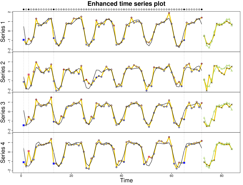
Figure 2: Enhanced time series plot obtained by applying RODESSA to the Electricity Load Diagrams data.

At the top of the plot we see circles reflecting the casewise weights $w_{r,i}$  with weight 1 shown with a white interior and lower weights in increasingly darker grey. A case $\bm{x}_{i}$ is flagged as a casewise outlier if $w_{r,i}$ is below the $\alpha$-quantile $q_{r,\alpha}$ of the simulated distribution of casewise weights at the reference model. Casewise outliers are indicated by a black solid circle and a vertical dashed grey line. The last one in the plot would not have been flagged in the cellwise way.

In this example we also want to plot the forecasts, which is not part of the default enhanced time series plot. The forecasts are shown as green triangles connected by green solid lines. The true values (which the algorithm did not know about) were added as black crosses connected by yellow solid lines, illustrating the forecasting performance.

4 Simulation study

In this section, the performance of the proposed RODESSA method in the presence of cellwise and casewise outliers is assessed through a Monte Carlo simulation study. The data generation process is inspired by the simulated example in Section 3.3 of Golyandina et al. (2018). Specifically, the multivariate time series is generated through the following signal plus noise model

$$x_{i}^{(j)}=s^{(j)}(i)+\varepsilon_{i}\quad\quad\text{for }i=1,\dots,N,\quad j=1,\dots,p\,,$$

with

$$s^{(j)}(i)=A^{(j)}\cos(2\pi i/10+C^{(j)})\,,$$

where $\varepsilon_{i}\sim N(0,\sigma^{2})$, $\sigma=20$, $p=4$, and $N=70$. The constants $A^{(j)}$ and $C^{(j)}$ are set according to the three scenarios in Table 1.

Table 1: Parameters $A^{(j)}$ and $C^{(j)}$ for scenarios 1, 2 and 3.

		Scenario 1			Scenario 2			Scenario 3
$j$		$A^{(j)}$	$C^{(j)}$		$A^{(j)}$	$C^{(j)}$		$A^{(j)}$	$C^{(j)}$
1		20	0		35	0		20	0
2		30	0		35	$\pi/5$		30	$\pi/5$
3		40	0		35	0		40	0
4		50	0		35	$\pi/5$		50	$\pi/5$

In each scenario we consider cellwise and casewise contamination settings, with the fraction of outliers $\varepsilon$ equal to $0.1$ and $0.2$. In the cellwise contamination setting, outliers are introduced by adding the number $\gamma\sigma$ to $\varepsilon pN$ randomly chosen values $x_{i}^{(j)}$. We let $\gamma$ range over $\gamma=0,1,\dots,8$, so $\gamma=0$ corresponds with the uncontaminated setting. In the casewise contamination setting, we add $\gamma\sigma$ to all values of $\varepsilon N$ randomly chosen $\bm{x}_{i}=(x_{i}^{(1)},\dots,x_{i}^{(4)})^{T}$.

Our proposed RODESSA method is compared with several competing approaches. We run the classical version of MSSA (labeled CMSSA) and several robust versions described in Section 2.3, which perform the decomposition step by (7) with $\rho(t)=|t|$ as in Rodrigues et al. (2018) (labeled RLM), as well as the method of Cheng et al. (2015) (labeled CHENG), and that of Chen and Sacchi (2015) (labeled CS).

RODESSA is implemented as described in Section 2 with $q=2$, which corresponds to the true rank since for any angle $\varphi$ the signal $A\cos(2\pi i/10+\varphi)$ equals the linear combination$A\cos(2\pi i/10)\cos(\varphi)-A\sin(2\pi i/10)\sin(\varphi)$ of the functions $\cos(\varphi)$ and $\sin(\varphi)$. Figure 3 plots the objective function for increasing rank, which also indicates that most of the variability is explained by two components. We consider both $L=56\simeq pN/(p+1)$ and $L=35=N/2$, and choose the tuning constants by setting $\delta_{c}=\delta_{r}=0.90$.

Figure 3: Graph of the objective function for increasing values of the rank $r$.

The competing approaches are implemented with the same values of $q$ and $L$. To guarantee a fair comparison between RODESSA and CS, the tuning parameter in the CS method is chosen by means of the procedure in Section 2.6. For each combination of scenario, contamination setting, magnitude $\gamma$ and outlier fraction, 2000 replications are carried out. The performance is assessed by means of the reconstruction error (RE) and the $20$-step ahead forecasting error (FE) that are defined as

$$\text{RE}=\frac{1}{pN}\sum_{j=1}^{p}\sum_{i=1}^{N}\left(\hat{x}_{i}^{j}-s^{j}(i)\right)^{2}\quad\quad\ \quad\text{FE}=\frac{1}{20p}\sum_{j=1}^{p}\sum_{i=N+1}^{N+20}\left(\hat{x}_{i}^{j}-s^{j}(i)\right)^{2}\;.$$ (21)

In the first formula the $\hat{x}_{i}^{j}$ are the reconstructions $(i\leqslant N)$. In the second formula they are the forecasts ($i>N$) as defined in (20). The RE and FE are then averaged over the replications.

We report the results for the most challenging Scenario 3, with $L=N/2$. The supplementary material contains the simulation results for the other settings, which yield qualitatively similar conclusions.

For cellwise contamination, Figure 4 shows the average RE and FE as a function of the contamination magnitude $\gamma$ for both outlier fractions. Without contamination ($\gamma=0$), CMSSA is the best method in terms of average RE and FE, as expected in this situation. But the errors of RODESSA and CS are similarly small, whereas those of CHENG and RLM are larger.

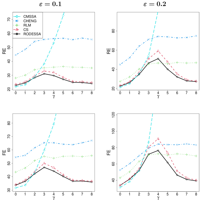
Figure 4: Cellwise outliers. Average RE (top) and FE (bottom) attained by CMSSA, CHENG, RLM, CS, and RODESSA for Scenario 3, contamination probability $\varepsilon=0.1$ (left) and $\varepsilon=0.2$ (right), as a function of $\gamma$.

When looking at increasing $\gamma>0$ it appears that far outlying cells have an unbounded effect on CMSSA, a bounded effect on CHENG and RLM, and a small effect on RODESSA and CS, due to their bounded biweight $\rho$ function. In that sense RODESSA and CS are similar. But RODESSA does better than CS, due to the fact that its decomposition step takes the diagonal structure of the Hankel matrix into account. The performance difference is largest for the higher outlier fraction $\varepsilon=0.2$.

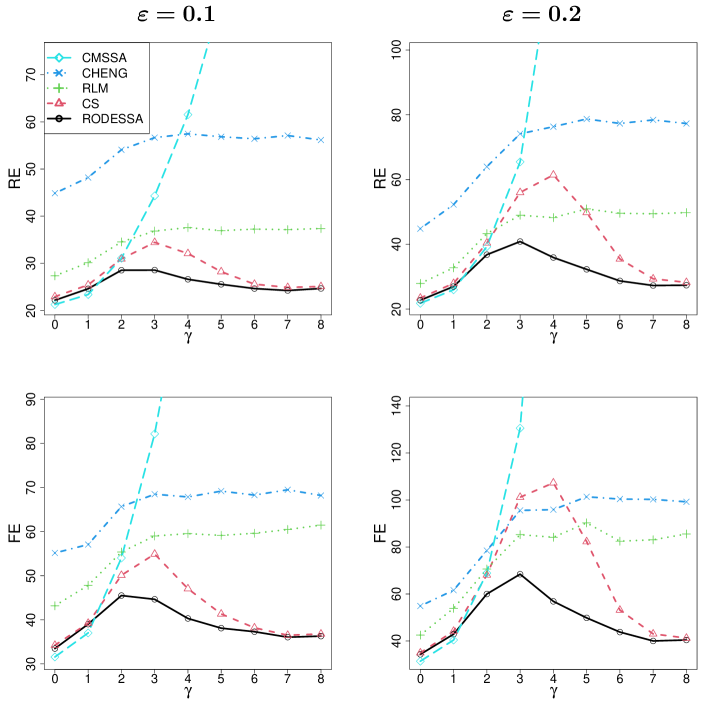
Figure 5: Casewise outliers. Average RE (top) and FE (bottom) attained by CMSSA, CHENG, RLM, CS, and RODESSA for Scenario 3, contamination probability $\varepsilon=0.1$ (left) and $\varepsilon=0.2$ (right), as a function of $\gamma$.

Figure 5 compares the same methods in the presence of casewise outliers. Here the differences are larger, with RODESSA outperforming the other methods more strongly. This is due to the fact that RODESSA can share information about diagonals across the stacked structure. This helps because we saw in Figure 1 that casewise outliers affect several diagonals in the trajectory matrix simultaneously. Unlike the other methods, RODESSA combines information across such diagonals through the loss function $\rho_{2}$ in (10), which makes it more robust for casewise outliers.

5 A real data example: temperature analysis in passenger railway vehicles

In this section, a real data example from the railway industry illustrates the applicability and potential of RODESSA.

In recent years, railway transportation in Europe has emerged as a viable alternative to other modes of transport, leading to intense competition between operators to enhance passenger satisfaction (Kallas, 2011). A particular challenge in this context is ensuring optimal thermal comfort inside passenger rail coaches (Ye et al., 2004). To address this challenge, new European standards, such as UNI EN 14750 (British Standards Institution, 2006), have been developed. These standards focus on regulating air temperature, relative humidity, air speed, and overall comfort and air quality in passenger rail coaches, taking into account the diverse operating requirements of trains. Consequently, railway companies are proactively installing sensors to gather and analyze data from on-board heating, ventilation, and air conditioning (HVAC) systems (Homod, 2013). HVAC systems play a crucial role in maintaining passenger thermal comfort, and their performance is being improved based on the insights obtained from the collected data.

We analyze operational data from HVAC systems installed on a passenger 6-coach train operating during the summer season (Lepore et al., 2022). The data are publicly available at https://github.com/unina-sfere/NN4MSP . Specifically, the inside temperature of each coach was recorded about every four minutes from 10:00 to 22:00, yielding $N=176$ observations of a multivariate time series with $p=6$ components. We applied RODESSA in its default form as described in Section 2.6, with $L=151\simeq pN/(p+1)$. We selected $q=7$ based on the values of the objective function. This yields the enhanced time series plot shown in Figure 6.

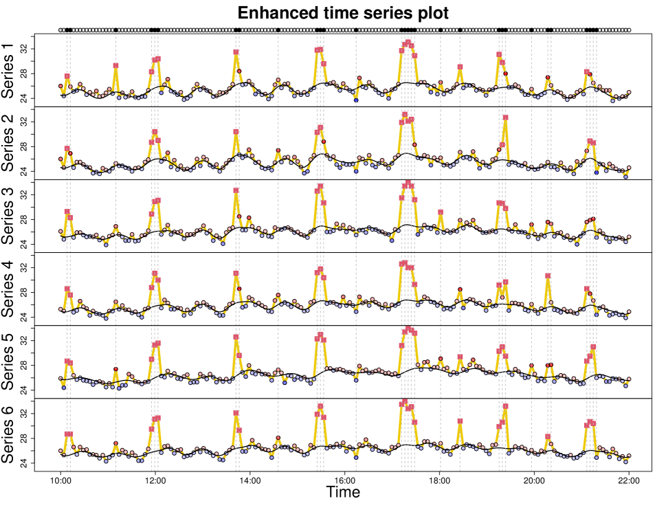
Figure 6: Enhanced time series plot from applying RODESSA to the multivariate time series of temperatures.

The vertical dashed lines in Figure 6 indicate casewise outliers. It seems that the temperature inside the six coaches is significantly higher than expected in an almost periodic fashion. This behavior is particularly severe for the group of casewise outliers between 17:00 and 18:00. Discussions with domain experts revealed that those measurements were acquired during train stops at terminal stations. In this situation the coach doors were left open, and due to the summer season this increased the temperature inside the coaches. From this we can conclude that those measurements are not representative of the operating conditions of the train and are not useful to characterize temperature dynamics. Moreover, the reconstructed time series shows that the temperature inside coaches does increase and decrease periodically, which is in accordance with the on/off control of the HVAC system. Note that not all casewise outliers are labeled as cellwise outliers. For instance, the casewise outlier shortly after 16:00 has no component that is flagged as a cellwise outlier, but the temperatures were relatively low in all six coaches simultaneously. The ability to detect such effects is a feature of the proposed method.

To assess the forecasting performance of RODESSA relative to the competing methods described in Section 4, we used subsequences of the multivariate time series. Specifically, starting from the first 120 observations, $h$-step ahead forecasts of all methods are computed for $h=5,10,20$. Similarly, forecasts are obtained by considering the first 121, 122,… observations and so on. For each subsequence, the $h$-step ahead forecasts are compared to the observed values of the time series, by computing the median of their absolute differences, denoted as mFE. Note that here we do not use the forecasting error formula in (21) because the data we are predicting contains outliers as well.

Moreover, to assess the effect of the window length $L$ on the forecasting performance we compare the two lengths given in Section 2.6, namely $1/2$ and $6/7$ of the subsequence length $N_{sub}$ . Figure 7 shows boxplots of mFE for $h=5,10,20$ and $L=N_{sub}/2$ (top) as well as $L=6N_{sub}/7$ (bottom). The RODESSA method outperforms its competitors overall, which is in line with the simulation study.

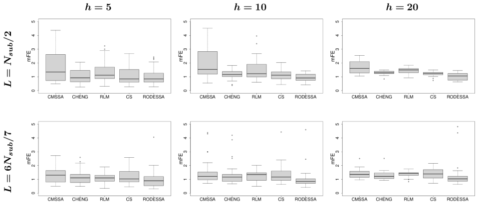
Figure 7: Boxplots of mFE for $h=5$, $10$, $20$ and $L=N_{sub}/2$ (top) as well as $L=6N_{sub}/7$ (bottom).

6 Conclusions

Multivariate singular spectrum analysis (MSSA) is a technique for fitting vector time series and making forecasts. It starts by constructing a matrix with a special structure. It consists of several submatrices stacked side by side, one for each component of the multivariate time series. A cell of the time series, that is, the value of one of its coordinates at a given timepoint, corresponds to a diagonal in the corresponding submatrix. A case of the time series, that is, all of the coordinates at a given time point, corresponds to diagonals in all of the submatrices.

Sometimes cells are outlying, and sometimes entire cases. But the classical MSSA method can be strongly affected by outliers, because it is based on a low-rank singular value decomposition, which is a least squares fit. Several more robust methods have been proposed in the literature, based on versions of the SVD that are less sensitive to outliers. However, these versions do not take the diagonal structure into account, and even a small number of outliers can create a large number of outlying diagonal entries that affect many rows and columns of the matrix, thereby overwhelming the fit. To resolve this issue we propose the RODESSA method, which explicitly takes the diagonal structure into account when decomposing the matrix. This makes it more robust than its predecessors, as illustrated in the extensive simulation study reported in Section 4 and the Supplementary Material. Moreover, it loses little efficiency when there are no outliers.

The RODESSA method is performed by a fast algorithm based on iteratively reweighted least squares. In Section 2 we prove a proposition stating that each step of the algorithm decreases the objective function. We also propose a new graphical display, called the enhanced time series plot, which visualizes the weights of the cells as well as the cases, making outliers stand out. We have applied the RODESSA method to a real multivariate time series about temperatures in passenger railway vehicles. This illustrates its good forecasting performance, as well as the convenient outlier detection by the enhanced time series plot.

Software availability.

The R code and example scripts, and the data of the example in Section 5, are publicly available on the webpage https://wis.kuleuven.be/statdatascience/robust .

Funding Details.

This work was supported by the Flanders Research Foundation (FWO) under Grant for a scientific stay in Flanders V505623N; and by Piano Nazionale di Ripresa e Resilienza (PNRR) - Missione 4 Componente 2, Investimento 1.3-D.D. 1551.11-10-2022, PE00000004 within the Extended Partnership MICS (Made in Italy - Circular and Sustainable).

A.1   Proof of Proposition 1

In this section Proposition 1 is proved, which ensures that each step of the algorithm decreases the RODESSA objective function (10). In order to prove Proposition 1, we first need two lemmas.

We will denote a potential fit as $\bm{\theta}=\bm{\widehat{X}}=\bm{U}\bm{V}^{T}$ where $\bm{\theta}$ belongs to the set of all $L\times K$ matrices of rank at most $q$. We introduce the notation $\bm{f}(\bm{\theta})$ for the column vector $\left(f_{1}(\bm{\theta}),\dots,f_{LK}(\bm{\theta})\right)^{T}$ with $LK$ entries, which are the values $(\bm{X}_{\ell k}-\bm{\theta}_{\ell k})^{2}$ for $\ell=1,\ldots,L$ and $k=1,\ldots,K$. We can then write the RODESSA objective function (10) as $L(\bm{f}(\bm{\theta})):=L_{\rho_{1},\rho_{2}}(\bm{X}-\bm{\theta})$.

Lemma 1.

The function $\bm{f}\rightarrow L(\bm{f})$ is concave.

Proof.

We first show that the univariate function $\rho:\mathbb{R}_{+}\rightarrow\mathbb{R}_{+}:t\rightarrow\rho_{c}(\sqrt{t})$, in which $\rho_{c}$ is Tukey’s biweight function (8), is concave. From $\rho(t)=1-(1-t/c^{2})^{3}I(0\leqslant t\leqslant c^{2})$ we can compute the second derivative

$$\rho^{\prime\prime}(t)\;=\;\frac{-6}{c^{4}}\left(1-\frac{t}{c^{2}}\right)I(0\leqslant t\leqslant c^{2})\;\leqslant\;0$$

from which concavity follows. The functions $\rho_{1}$ and $\rho_{2}$ in RODESSA are thus concave.

By the definition of concavity of a multivariate function, we now need to prove that for any column vectors $\bm{f},\bm{g}$ in $\mathbb{R}_{+}^{LK}$ and any $\lambda$ in $\left(0,1\right)$ it holds that $L(\lambda\bm{f}+(1-\lambda)\bm{g})\geqslant\lambda L(\bm{f})+(1-\lambda)L(\bm{g})$. This works out as

$$L(\lambda\bm{f}+(1-\lambda)\bm{g})=$$

$$\sum_{i=1}^{N}pn_{i}\hat{\sigma}_{2}^{2}\rho_{2}\left(\frac{\sum_{j=1}^{p}n_{i}\hat{\sigma}_{1,j}^{2}\rho_{1}\left(\sum_{a=1}^{n_{i}}(\lambda f_{ia}^{(j)}+(1-\lambda)g_{ia}^{(j)})/(n_{i}\hat{\sigma}_{1,j}^{2})\right)}{pn_{i}\hat{\sigma}_{2}^{2}}\right)\geqslant$$

$$\sum_{i=1}^{N}pn_{i}\hat{\sigma}_{2}^{2}\rho_{2}\left(\frac{\sum_{j=1}^{p}n_{i}\hat{\sigma}_{1,j}^{2}\left[\lambda\rho_{1}\left(\sum_{a=1}^{n_{i}}f_{ia}^{(j)}/(n_{i}\hat{\sigma}_{1,j}^{2})\right)+(1-\lambda)\rho_{1}\left(\sum_{a=1}^{n_{i}}g_{ia}^{(j)}/(n_{i}\hat{\sigma}_{1,j}^{2})\right)\right]}{pn_{i}\hat{\sigma}_{2}^{2}}\right)=$$

$$\sum_{i=1}^{N}pn_{i}\hat{\sigma}_{2}^{2}\rho_{2}\left(\frac{\lambda\sum_{j=1}^{p}n_{i}\hat{\sigma}_{1,j}^{2}\rho_{1}\left(\sum_{a=1}^{n_{i}}f_{ia}^{(j)}/(n_{i}\hat{\sigma}_{1,j}^{2})\right)+(1-\lambda)\sum_{j=1}^{p}n_{i}\hat{\sigma}_{1,j}^{2}\rho_{1}\left(\sum_{a=1}^{n_{i}}g_{ia}^{(j)}/(n_{i}\hat{\sigma}_{1,j}^{2})\right)}{pn_{i}\hat{\sigma}_{2}^{2}}\right)\geqslant$$

$$\sum_{i=1}^{N}pn_{i}\hat{\sigma}_{2}^{2}\left[\lambda\rho_{2}\left(\frac{\sum_{j=1}^{p}n_{i}\hat{\sigma}_{1,j}^{2}\rho_{1}\left(\sum_{a=1}^{n_{i}}f_{ia}^{(j)}/(n_{i}\hat{\sigma}_{1,j}^{2})\right)}{pn_{i}\hat{\sigma}_{2}^{2}}\right)\right.$$

$$\left.\hskip 142.26378pt+\,(1-\lambda)\rho_{2}\left(\frac{\sum_{j=1}^{p}n_{i}\hat{\sigma}_{1,j}^{2}\rho_{1}\left(\sum_{a=1}^{n_{i}}g_{ia}^{(j)}/(n_{i}\hat{\sigma}_{1,j}^{2})\right)}{pn_{i}\hat{\sigma}_{2}^{2}}\right)\right]=$$

$$\lambda L(\bm{f})+(1-\lambda)L(\bm{g}).$$

The first inequality derives from the concavity of $\rho_{1}$ and the fact that $\rho_{2}$ is nondecreasing. The second inequality is due to the concavity of $\rho_{2}$ . Therefore $L$ is a concave function. ∎

We can also write the weighted least squares objective (17) as a function of $\bm{f}$. We will denote it as $L_{\bm{W}}(\bm{f}):=(\operatorname{vec}(\bm{W}))^{T}\bm{f}$. Here $\operatorname{vec}(.)$ turns a matrix into a column vector, in the same way as was done to obtain the column vector $\bm{f}$. The next lemma makes a connection between $L_{\bm{W}}$ and the RODESSA objective $L$.

Lemma 2.

If two column vectors $\bm{f},\bm{g}$ in $\mathbb{R}_{+}^{LK}$ satisfy $L_{\bm{W}}(\bm{f})\leqslant L_{\bm{W}}(\bm{g})$, then $L(\bm{f})\leqslant L(\bm{g})$.

Proof.

From Lemma 1 we know that $L(\bm{f})$ is concave as a function of $\bm{f}$, and it is also differentiable because $\rho_{1}$ and $\rho_{2}$ are. Therefore

$$L(\bm{f})\leqslant L_{(}\bm{g})+(\nabla L(\bm{g}))^{T}(\bm{f}-\bm{g})$$

where the column vector $\nabla L(\bm{g})$ is the gradient of $L$ in $\bm{g}$. But $\nabla L(\bm{g})$ equals $\operatorname{vec}(\bm{W})$ byconstruction, so $(\nabla L(\bm{g}))^{T}(\bm{f}-\bm{g})=L_{\bm{W}}(\bm{f})-L_{\bm{W}}(\bm{g})\leqslant 0$. Therefore $L(\bm{f})\leqslant L(\bm{g})$. ∎

With this preparation we can prove Proposition 1.

Proof of Proposition 1.

When we go from $\bm{\theta}_{t}$ to $\bm{\theta}_{t+1}$ the least squares fits in steps 5 and 6of Algorithm 1 ensure that $L_{\bm{W}_{t}}(\bm{f}(\bm{\theta}_{t+1}))\leqslant L_{\bm{W}_{t}}(\bm{f}(\bm{\theta}_{t}))$, so it follows from Lemma 2 that$L(\bm{f}(\bm{\theta}_{t+1}))\leqslant L(\bm{f}(\bm{\theta}_{t}))$. ∎

A.2   Additional simulation results

In this section we present all the simulation results according to the settings described in Section 4. In the uncontaminated setting ($\gamma=0$), Figure 8 shows examples of multivariate time series generated by scenarios 1, 2 and 3. Scenario 1 generates series in which the components have increasing amplitude, whereas Scenario 2 shifts their phase. Scenario 3 combines both effects.

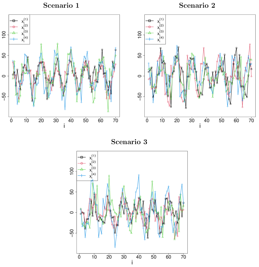
Figure 8: (No outliers.) Examples of randomly generated multivariate time series under scenarios 1, 2, and 3 of the simulation study.

We first consider the window length $L=N/2=35$. Figure 9 shows the average RE and FE for each scenario (S1, S2 and S3) and outlier fraction $\varepsilon$ as a function of $\gamma$, for data with cellwise contamination. Figure 10 does the same for casewise contamination.

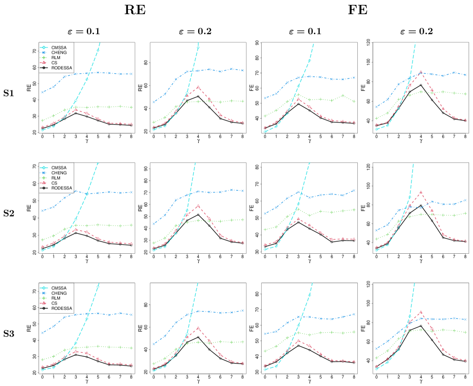
Figure 9: (Window length $L=35$, cellwise outliers.) Average RE and FE attained by CMSSA, CHENG, RLM, CS, and RODESSA for each scenario (S1, S2, and S3) and contamination probability ($\varepsilon=0.1,0.2$) in function of $\gamma$.

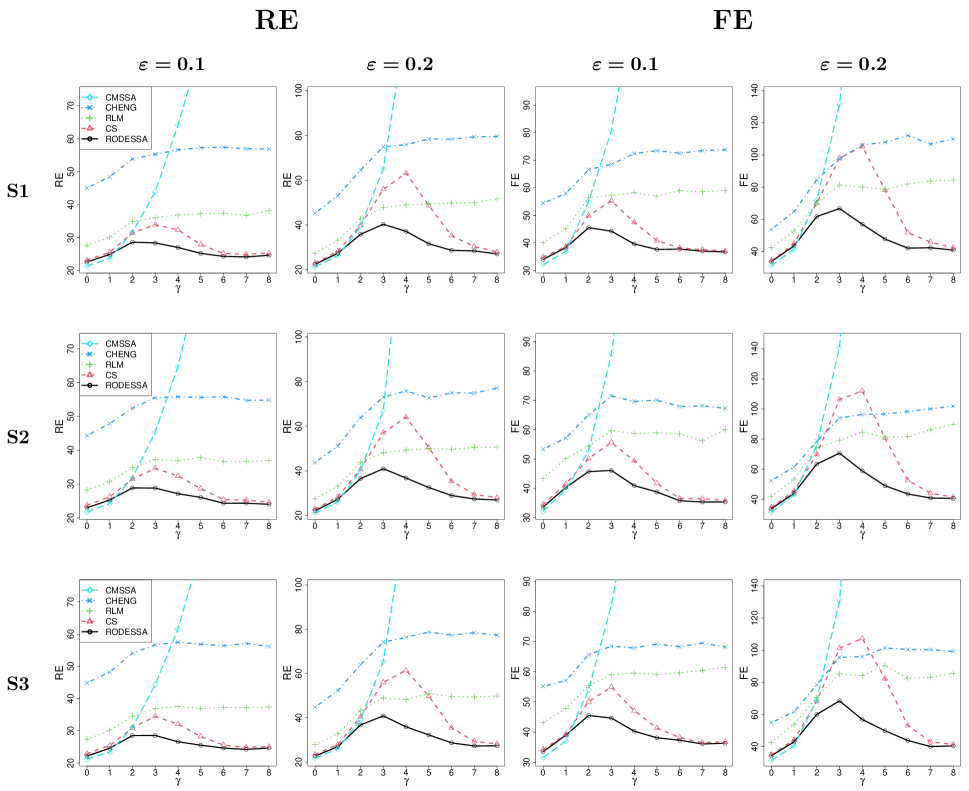
Figure 10: (Window length $L=35$, casewise outliers.) Average RE and FE attained by CMSSA, CHENG, RLM, CS, and RODESSA for each scenario (S1, S2, and S3) and contamination probability ($\varepsilon=0.1,0.2$) in function of $\gamma$.

Figures 11 and 12 show the corresponding results for window length $L=56\sim pN/(p+1)$.

We conclude that all these simulation results are qualitatively similar to those reported in Section 4 of the paper.

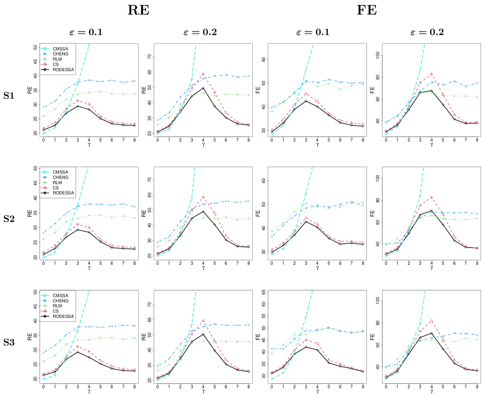
Figure 11: (Window length $L=56$, cellwise outliers.) Average RE and FE attained by CMSSA, CHENG, RLM, CS, and RODESSA for each scenario (S1, S2, and S3) and contamination probability ($\varepsilon=0.1,0.2$) in function of $\gamma$.

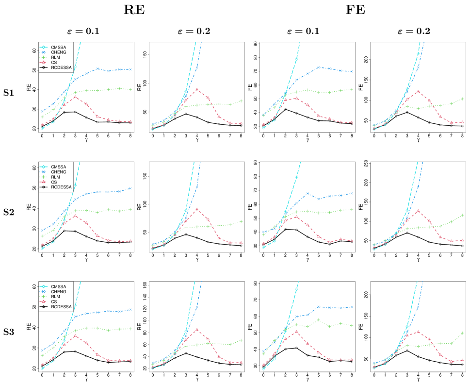
Figure 12: (Window length $L=56$, casewise outliers.) Average RE and FE attained by CMSSA, CHENG, RLM, CS, and RODESSA for each scenario (S1, S2, and S3) and contamination probability ($\varepsilon=0.1,0.2$) in function of $\gamma$.

References

- Aeberhard et al. (2021) Aeberhard, W., E. Cantoni, G. Marra, and R. Radice (2021). Robust fitting for generalized additive models for location, scale and shape. Statistics and Computing 31, 11.
- Alqallaf et al. (2009) Alqallaf, F., S. Van Aelst, V. J. Yohai, and R. H. Zamar (2009). Propagation of outliers in multivariate data. The Annals of Statistics 37, 311–331.
- British Standards Institution (2006) British Standards Institution (2006). BS-EN 14750: Railway applications – Air conditioning for urban and suburban rolling stock. Part 1: Comfort parameters.
- Broomhead and King (1986) Broomhead, D. and G. King (1986). On the qualitative analysis of experimental dynamical systems. In S. Sarkar (Ed.), Nonlinear Phenomena and Chaos, pp. 113–144. Hilger Ltd.
- Candès et al. (2011) Candès, E. J., X. Li, Y. Ma, and J. Wright (2011). Robust principal component analysis? Journal of the ACM 58(3), 1–37.
- Chen and Sacchi (2015) Chen, K. and M. D. Sacchi (2015). Robust reduced-rank filtering for erratic seismic noise attenuation. Geophysics 80(1), V1–V11.
- Cheng et al. (2015) Cheng, J., K. Chen, and M. D. Sacchi (2015). Application of Robust Principal Component analysis (RPCA) to suppress erratic noise in seismic records. In SEG Technical Program Expanded Abstracts 2015, pp. 4646–4651. Society of Exploration Geophysicists.
- Croux et al. (2003) Croux, C., P. Filzmoser, G. Pison, and P. J. Rousseeuw (2003). Fitting multiplicative models by robust alternating regressions. Statistics and Computing 13, 23–36.
- Danilov (1997) Danilov, D. (1997). Principal components in time series forecast. Journal of Computational and Graphical Statistics 6(1), 112–121.
- De Klerk (2015) De Klerk, J. (2015). Time series outlier detection using the trajectory matrix in singular spectrum analysis with outlier maps and ROBPCA. South African Statistical Journal 49, 61–76.
- De la Torre and Black (2003) De la Torre, F. and M. J. Black (2003). A framework for robust subspace learning. International Journal of Computer Vision 54, 117–142.
- Gabriel (1978) Gabriel, K. R. (1978). Least squares approximation of matrices by additive and multiplicative models. Journal of the Royal Statistical Society: Series B (Methodological) 40(2), 186–196.
- Golyandina et al. (2018) Golyandina, N., A. Korobeynikov, and A. Zhigljavsky (2018). Singular spectrum analysis with R. Springer.
- Golyandina et al. (2001) Golyandina, N., V. Nekrutkin, and A. Zhigljavsky (2001). Analysis of time series structure: SSA and related techniques. CRC press.
- Golyandina and Zhigljavsky (2013) Golyandina, N. and A. Zhigljavsky (2013). Singular Spectrum Analysis for Time Series. Springer Berlin, Heidelberg.
- Hassani and Mahmoudvand (2013) Hassani, H. and R. Mahmoudvand (2013). Multivariate singular spectrum analysis: A general view and new vector forecasting approach. International Journal of Energy and Statistics 1(01), 55–83.
- Homod (2013) Homod, R. Z. (2013). Review on the HVAC system modeling types and the shortcomings of their application. Journal of Energy 2013, 1–10.
- Hubert et al. (2019) Hubert, M., P. J. Rousseeuw, and W. Van den Bossche (2019). MacroPCA: an all-in-one PCA method allowing for missing values as well as cellwise and rowwise outliers. Technometrics 61(4), 459–473.
- Hubert et al. (2005) Hubert, M., P. J. Rousseeuw, and K. Vanden Branden (2005). ROBPCA: a new approach to robust principal component analysis. Technometrics 47, 64–79.
- Kallas (2011) Kallas, S. (2011). White Paper on transport: Roadmap to a single European transport area: towards a competitive and resource-efficient transport system. Office for Official Publications of the European Communities.
- Lepore et al. (2022) Lepore, A., B. Palumbo, and G. Sposito (2022). Neural network based control charting for multiple stream processes with an application to HVAC systems in passenger railway vehicles. Applied Stochastic Models in Business and Industry 38(5), 862–883.
- Markovsky (2008) Markovsky, I. (2008). Structured low-rank approximation and its applications. Automatica 44, 891–909.
- Maronna et al. (2019) Maronna, R. A., R. D. Martin, V. J. Yohai, and M. Salibián-Barrera (2019). Robust Statistics: Theory and Methods (with R). John Wiley & Sons.
- Raymaekers and Rousseeuw (2021) Raymaekers, J. and P. J. Rousseeuw (2021). Fast robust correlation for high-dimensional data. Technometrics 63, 184–198.
- Raymaekers and Rousseeuw (2023) Raymaekers, J. and P. J. Rousseeuw (2023). Challenges of cellwise outliers. Econometrics and Statistics X, to appear.
- Rodrigues et al. (2018) Rodrigues, P. C., V. Lourenço, and R. Mahmoudvand (2018). A robust approach to singular spectrum analysis. Quality And Reliability Engineering International 34(7), 1437–1447.
- Rodrigues et al. (2020) Rodrigues, P. C., J. Pimentel, P. Messala, and M. Kazemi (2020). The decomposition and forecasting of mutual investment funds using singular spectrum analysis. Entropy 22(1), 83.
- Rousseeuw and Leroy (1987) Rousseeuw, P. J. and A. Leroy (1987). Robust Regression and Outlier Detection. Wiley.
- Rousseeuw and Van den Bossche (2018) Rousseeuw, P. J. and W. Van den Bossche (2018). Detecting deviating data cells. Technometrics 60(2), 135–145.
- Trindade (2015) Trindade, A. (2015). Electricity Load Diagrams 20112014. UCI Machine Learning Repository. DOI: https://doi.org/10.24432/C58C86.
- Ye et al. (2004) Ye, X., H. Lu, D. Li, B. Sun, and Y. Liu (2004). Thermal comfort and air quality in passenger rail cars. International Journal of Ventilation 3(2), 183–192.
- Zhang et al. (2013) Zhang, L., H. Shen, and J. Z. Huang (2013). Robust regularized singular value decomposition with application to mortality data. The Annals of Applied Statistics 7, 1540–1561.
Supplementary Material to: