Determination of $|V_{cb}|$ using ${\kern 1.79993pt\overline{\kern-1.79993ptB}}{}^{0}\to D^{*+}\ell^{-}\bar{\nu}_{\ell}$ decays with Belle II

Abstract

We determine the Cabibbo-Kobayashi-Maskawa matrix-element magnitude $|V_{cb}|$ using ${\kern 1.79993pt\overline{\kern-1.79993ptB}}{}^{0}\to D^{*+}\ell^{-}\bar{\nu}_{\ell}$ decays reconstructed in $189\,\mathrm{fb}^{-1}$ of collision data collected by the Belle II experiment, located at the SuperKEKB $e^{+}e^{-}$ collider. Partial decay rates are reported as functions of the recoil parameter $w$ and three decay angles separately for electron and muon final states. We obtain $|V_{cb}|$ using the Boyd-Grinstein-Lebed and Caprini-Lellouch-Neubert parametrizations, and find $|V_{cb}|_{\mathrm{BGL}}=(40.57\pm 0.31\pm 0.95\pm 0.58)\times 10^{-3}$ and $|V_{cb}|_{\mathrm{CLN}}=(40.13\pm 0.27\pm 0.93\pm 0.58)\times 10^{-3}$ with the uncertainties denoting statistical components, systematic components, and components from the lattice QCD input, respectively. The branching fraction is measured to be ${\cal B}({\kern 1.79993pt\overline{\kern-1.79993ptB}}{}^{0}\to D^{*+}\ell^{-}\bar{\nu}_{\ell})=(4.922\pm 0.023\pm 0.220)\%$. The ratio of branching fractions for electron and muon final states is found to be $0.998\pm 0.009\pm 0.020$. In addition, we determine the forward-backward angular asymmetry and the $D^{*+}$ longitudinal polarization fractions. All results are compatible with lepton-flavor universality in the Standard Model.

I Introduction

In the Standard Model (SM) of particle physics, the Cabibbo-Kobayashi-Maskawa (CKM) matrix relates the weak interaction and mass eigenstates of quarks [1, 2]. It is a $3\times 3$ unitary complex matrix and currently the only established source for charge-parity (CP) violating processes in the SM. The elements of the CKM matrix are free parameters of the SM and need to be determined experimentally. In this paper, we report the determination of the magnitude of the CKM matrix element $V_{cb}$ with Belle II data. The values of $|V_{cb}|$ should be consistent when determined using different physics processes involving $b\to c$ quark transitions. However, a longstanding discrepancy between inclusive and exclusive determinations is observed, cf. Ref. [3]. Reference [4] combines measurements of exclusive $B\to D^{(*)}\ell\bar{\nu}_{\ell}$ and $B^{0}_{s}\to D_{s}^{(*)-}\,\ell^{+}\nu_{\ell}$ decays, where $\ell=e,\mu$, and $B$ and $D$ indicate charged and neutral bottom and charmed mesons, respectively. This combination results in a value of

$$|V_{cb}|=(39.10\pm 0.50)\times 10^{-3}\quad(\text{exclusive}).$$ (1)

The most precise inclusive determination combines measured spectral moments of lepton energy and hadronic invariant-mass spectra with measurements of partial branching fractions and calculations of the total rate at next-to-next-to-next-to-leading order in the strong interaction [5],

$$|V_{cb}|=(42.16\pm 0.51)\times 10^{-3}\quad(\text{inclusive}).$$ (2)

Alternative inclusive determinations obtain a similar value using lepton-mass squared moments [6, 7, 8, 9].

In this paper, we examine the semileptonic ${\kern 1.79993pt\overline{\kern-1.79993ptB}}{}^{0}\to D^{*+}\ell^{-}\bar{\nu}_{\ell}$ decay, which is a usual benchmark channel to determine $|V_{cb}|$ due to the sizeable branching fraction, small backgrounds, and the availability of lattice QCD (LQCD) information at and beyond zero recoil [10, 11, 12, 13]. LQCD inputs aid in disentangling the normalization of the hadronic-transition form factors, which describe the nonperturbative processes of the strong interaction in the $B\to D^{(*)}$ transition.

Aside from the $|V_{cb}|$ discrepancies, several observations suggest a possible deviation from the SM’s lepton-flavor universality (LFU) in semileptonic $B$ decays (see, e.g.,  [14, 15] for recent reviews). For example, the combined averages of ${\cal R}(D)$ and ${\cal R}(D^{*})$ are about three standard deviations larger than the SM expectation [4], where

$${\cal R}(D^{(*)})=\frac{{\cal B}(B\rightarrow D^{(*)}\tau\bar{\nu}_{\tau})}{{\cal B}(B\rightarrow D^{(*)}\ell\bar{\nu}_{\ell})},\quad\text{with }\ell=e,\,\mu\,.$$ (3)

This ratio does not depend on $|V_{cb}|$, but the most precise predictions rely on measurements of the form factors. In addition, a reanalysis [16] of Belle data [17] recently extracted the difference of the forward-backward angular asymmetry between electrons and muons in ${\kern 1.79993pt\overline{\kern-1.79993ptB}}{}^{0}\to D^{*+}\ell^{-}\bar{\nu}_{\ell}$ decays and observed a significant tension of about four standard deviations with the SM expectation. Motivated by this, the Belle II collaboration carried out tests of LFU with the same decay channels using events where the accompanying $B$ meson is fully reconstructed in hadronic modes [18].

In this work, we exploit an independent dataset to further study LFU in ${\kern 1.79993pt\overline{\kern-1.79993ptB}}{}^{0}\to D^{*+}\ell^{-}\bar{\nu}_{\ell}$ decays, and to measure the form factors, which are essential to predict ${\cal R}(D^{(*)})$ within and beyond the SM.

We reconstruct ${\kern 1.79993pt\overline{\kern-1.79993ptB}}{}^{0}\to D^{*+}\ell^{-}\bar{\nu}_{\ell}$ decays with the subsequent $D^{*+}\to D^{0}\pi^{+}$ and $D^{0}\to K^{-}\pi^{+}$ decays, without explicit reconstruction of the other $B$ meson produced in the $e^{+}e^{-}\to\Upsilon(4S)\to B^{0}{\kern 1.79993pt\overline{\kern-1.79993ptB}}{}^{0}$ process. The measurement uses $189\,\mathrm{fb}^{-1}$ of data recorded by the Belle II experiment. A novel approach is developed to reconstruct the four kinematic variables that fully describe the ${\kern 1.79993pt\overline{\kern-1.79993ptB}}{}^{0}\to D^{*+}\ell^{-}\bar{\nu}_{\ell}$ decay. We report partial decay rates in intervals (bins) of these kinematic variables corrected for detector distortions and acceptance effects. Furthermore, we report the total rate, the values of the form factors, and $|V_{cb}|$.

The remainder of this paper is organized as follows. Section II introduces the theoretical formalism of ${\kern 1.79993pt\overline{\kern-1.79993ptB}}{}^{0}\to D^{*+}\ell^{-}\bar{\nu}_{\ell}$ decays and the measured observables. An overview of the Belle II subdetectors and the dataset is given in Sec. III. In Secs. IV and V, we summarize the event selection and the reconstruction of the four kinematic variables. Section VI details the signal extraction and unfolding procedure and Sec. VII lists the systematic uncertainties affecting the measurement. The measured value of $|V_{cb}|$ and form-factor parameters are discussed in Sec. VIII. Finally, Sec. IX presents a summary and our conclusions.

II Theory of ${\kern 1.79993pt\overline{\kern-1.79993ptB}}{}^{0}\to D^{*+}\ell^{-}\bar{\nu}_{\ell}$ decays

In the SM and the heavy-quark symmetry basis [19, 20], the transition between $B$ and $D^{*}$ mesons is represented in terms of four independent form factors $h_{A_{1-3},V}$,

$$\frac{\langle D^{*}(p_{D^{*}})|\bar{c}\gamma^{\mu}b|\bar{B}(p_{B})\rangle}{\sqrt{m_{B}m_{D^{*}}}}=~{} i~{}h_{V}\,\varepsilon^{\mu\nu\alpha\beta}\,\epsilon^{*}_{\nu}\,v^{\prime}_{\alpha}\,v_{\beta}\,,$$ (4)

$$\frac{\langle D^{*}(p_{D^{*}})|\bar{c}\gamma^{\mu}\gamma_{5}b|\bar{B}(p_{B})\rangle}{\sqrt{m_{B}m_{D^{*}}}}=~{} h_{A_{1}}\,(w+1)\,\epsilon^{*\mu}-h_{A_{2}}\,(\epsilon^{*}\cdot v)$$ (5)

$$\times v^{\mu}-h_{A_{3}}\,(\epsilon^{*}\cdot v)\,v^{\prime\mu}\,.$$

Here $v=p_{B}/m_{B}$ and $v^{\prime}=p_{D^{*}}/m_{D^{*}}$ are the four-velocities of $B$ and $D^{*}$ mesons, respectively, with $p_{B}$ and $p_{D^{*}}$ denoting four-momenta of $B$ and $D^{*}$ mesons, and $m_{B}$ and $m_{D^{*}}$ denoting masses of $B$ and $D^{*}$ mesons, respectively. Further, $\epsilon^{*}$ is the polarization of the $D^{*}$ meson and $\varepsilon^{\mu\nu\alpha\beta}$ is the Levi-Civita tensor. The four form factors $h_{A_{1-3},V}$ parametrize the nonperturbative physics of the $B\to D^{*}$ transition as functions of the recoil parameter $w=v\cdot v^{\prime}$, which is related to the squared four-momentum transferred from the $B$ meson to the $D^{*}$ meson as

$$q^{2}=\left(p_{B}-p_{D^{*}}\right)^{2}=m_{B}^{2}+m_{D^{*}}^{2}-2m_{B}\,m_{D^{*}}\,w\,.$$ (6)

In the light lepton mass limit, the ${\kern 1.79993pt\overline{\kern-1.79993ptB}}{}^{0}\to D^{*+}\ell^{-}\bar{\nu}_{\ell}$ decay is fully described by $h_{A_{1}}$ and two form-factor ratios,

$$R_{1}=\frac{h_{V}}{h_{A_{1}}}\,,\qquad R_{2}=\frac{h_{A_{3}}+r^{*}h_{A_{2}}}{h_{A_{1}}}\,,$$ (7)

with $r^{*}=m_{D^{*}}/m_{B}$.

An alternative parametrization is given by the helicity basis [21, 22]. The three form factors in this basis, $g,f$, and ${\cal F}_{1}$ are related to the heavy-quark basis via

$$f =m_{B}\sqrt{r^{*}}(w+1)\,h_{A_{1}}\,,\qquad g=\frac{1}{m_{B}\sqrt{r^{*}}}\,R_{1}\,h_{A_{1}}\,,$$ (8)

$${\cal F}_{1} =m_{B}^{2}\,\sqrt{r^{*}}(w+1)\left(w-r^{*}-(w-1)R_{2}\right)\,h_{A_{1}}.$$ (9)

The ${\kern 1.79993pt\overline{\kern-1.79993ptB}}{}^{0}\to D^{*+}\ell^{-}\bar{\nu}_{\ell}$ decay rate is fully parametrized by the recoil parameter $w$ and three decay angles $\theta_{\ell}$, $\theta_{V}$, and $\chi$, defined as follows (see also Fig. 1).

• The angle $\theta_{\ell}$ is the angle between the direction of the charged lepton and the direction opposite to the $B$ meson in the virtual $W$ boson rest frame.

• The angle $\theta_{V}$ is the angle between the direction of the $D$ meson and the direction opposite to the $B$ meson in the $D^{*}$ meson rest frame.

• The angle $\chi$ is the azimuthal angle between the two decay planes spanned by the $W$ boson and $D^{*}$ meson decay products, and defined in the rest frame of the $B$ meson.

Integrating over the angles, the ${\kern 1.79993pt\overline{\kern-1.79993ptB}}{}^{0}\to D^{*+}\ell^{-}\bar{\nu}_{\ell}$ decay rate is expressed as

$$\frac{\mathrm{d}\Gamma({\kern 1.79993pt\overline{\kern-1.79993ptB}}{}^{0}\to D^{*+}\ell^{-}\bar{\nu}_{\ell})}{\mathrm{d}w} =\frac{G_{F}^{2}|V_{cb}|^{2}\,\eta_{\rm EW}^{2}\,m_{B}^{5}c^{4}}{48\pi^{3}\hbar^{7}}\,$$

$$\quad\times(w^{2}-1)^{1/2}\,(w+1)^{2}\,r^{*3}(1-r^{*})^{2}$$

$$\quad\times\bigg{[}1+\frac{4w}{w+1}\frac{1-2wr^{*}+r^{*2}}{(1-r^{*})^{2}}\bigg{]}\mathcal{F}(w)^{2}\,,$$ (10)

with $G_{F}$ and $\eta_{\rm EW}\simeq 1.0066$ [23] denoting the Fermi coupling constant and electroweak correction, respectively, and

$$\mathcal{F}(w)^{2} =h_{A_{1}}^{2}\bigg{\{}2(1-2wr^{*}+r^{*2})\bigg{(}1+R_{1}^{2}\,\frac{w-1}{w+1}\bigg{)}$$

$$\qquad\qquad\qquad+\big{[}(1-r^{*})+(w-1)\big{(}1-R_{2}\big{)}\big{]}^{2}\bigg{\}}$$

$$\qquad\quad\times\bigg{[}(1-r^{*})^{2}+\frac{4w}{w+1}\big{(}1-2wr^{*}+r^{*2}\big{)}\bigg{]}^{-1}\,.$$ (11)

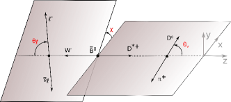
Figure 1: Sketch of the helicity angles $\theta_{\ell}$, $\theta_{V}$, and $\chi$ that characterize the ${\kern 1.79993pt\overline{\kern-1.79993ptB}}{}^{0}\to D^{*+}\ell^{-}\bar{\nu}_{\ell}$ decay.

II.1 Boyd-Grinstein-Lebed parametrization

References [22, 21] (Boyd, Grinstein, and Lebed; BGL) utilize dispersive bounds and expand the helicity-basis form factors with a conformal parameter,

$$z=\frac{\sqrt{w+1}-\sqrt{2}}{\sqrt{w+1}+\sqrt{2}}\,,$$ (12)

in terms of coefficients $\{a_{n},b_{n},c_{n}\}$ as [24]

$$g(z) =\frac{1}{P_{g}(z)\phi_{g}(z)}\sum^{n_{a}-1}_{n=0}a_{n}z^{n},$$ (13)

$$f(z) =\frac{1}{P_{f}(z)\phi_{f}(z)}\sum^{n_{b}-1}_{n=0}b_{n}z^{n},$$ (14)

$${\cal F}_{1}(z) =\frac{1}{P_{{\cal F}_{1}}(z)\phi_{{\cal F}_{1}}(z)}\sum^{n_{c}-1}_{n=0}c_{n}z^{n},\,$$ (15)

with $n_{a/b/c}$ the order of the expansion. Further, $P$ and $\phi$ denote the corresponding Blaschke factors and the outer functions, respectively. Note that in the expansion $b_{0}$ and $c_{0}$ are not independent quantities but related via

$$c_{0}=\left(\frac{\left(m_{B}-m_{D^{*}}\right)\phi_{{\cal F}_{1}}(0)}{\phi_{f}(0)}\right)b_{0}\,.$$ (16)

II.2 Caprini-Lellouch-Neubert parametrization

Reference [25] (Caprini, Lellouch, and Neubert; CLN) uses dispersive bounds and quark-model input to reduce the number of parameters required to describe the form factors. The form-factor $h_{A_{1}}$ is expanded in the conformal parameter $z$ [Eq. 12] with a single slope parameter $\rho^{2}$,

$$h_{A_{1}}(z)\,= \,h_{A_{1}}(w=1)\bigg{(}1-8\rho^{2}z+(53\rho^{2}-15)z^{2}$$ (17)

$$\qquad\qquad\qquad\qquad-(231\rho^{2}-91)z^{3}\bigg{)}.$$

The remaining form factors are parametrized using the ratios

$$R_{1}(w)\,= \,R_{1}(1)-0.12(w-1)+0.05(w-1)^{2},$$ (18)

$$R_{2}(w)\,= \,R_{2}(1)+0.11(w-1)-0.06(w-1)^{2}.$$ (19)

Therefore the form factors are fully parametrized by $\rho^{2},R_{1}(1)$, and $R_{2}(1)$.

III Belle II detector and data sample

The Belle II detector [26, 27] operates at the SuperKEKB asymmetric-energy electron-positron collider [28] and is located at the KEK laboratory. The detector consists of several nested detector subsystems arranged around the beam pipe in a cylindrical geometry. The innermost subsystem is the vertex detector, which includes two layers of silicon pixel detectors and four outer layers of silicon strip detectors. For the data used in this work, the outer pixel layer is installed in only a small part of the solid angle, while the remaining vertex-detector layers are fully instrumented. Most of the tracking volume consists of a helium and ethane-based small cell drift chamber (CDC). We define the $z$ axis parallel to the CDC axis of symmetry and directed along the boost direction. The azimuthal angle $\phi$ and the polar angle $\theta$ are defined with respect to this axis. The CDC covers a $\theta$ range between 17°and 150°and the full $\phi$ range. Outside the drift chamber, a time-of-propagation detector provides charged-particle identification in the barrel region, covering a polar angle $32.2\degree<\theta<128.7\degree$. In the forward end cap, covering a range of $12.4\degree<\theta<31.4\degree$, charged-particle identification is provided by a proximity-focusing, ring-imaging Cherenkov detector with an aerogel radiator (ARICH). Further out is the electromagnetic calorimeter (ECL) made of CsI(Tl) crystals. It consists of the barrel, forward end cap and backward end cap, which covers a range of $130.7\degree<\theta<155.1\degree$. An axial magnetic field is provided by a superconducting solenoid situated outside the calorimeter. Multiple layers of scintillators and resistive-plate chambers, located between the magnetic flux-return iron plates, constitute the $K^{0}_{L}$ and muon identification system (KLM).

This analysis uses data collected between 2019 and 2021 at a c.m. energy of $\sqrt{s}=10.58$ GeV and corresponding to an integrated luminosity of $189\,\mathrm{fb}^{-1}$. The energies of the electron and positron beams are $7$ and $4\,\mathrm{GeV}$, respectively. The number of $B$-meson pairs is determined, using event-shape variables, to be $N_{B{\kern 1.25995pt\overline{\kern-1.25995ptB}}}=\left(198\pm 3\right)\times 10^{6}$. In addition, $12\,\mathrm{fb}^{-1}$ of collision data recorded at a c.m. energy of 10.52 GeV are used to validate the modeling of continuum including $e^{+}e^{-}\to\tau^{+}\tau^{-}$ and $e^{+}e^{-}\to q\bar{q}$ processes, where $q$ indicates an $u$, $d$, $s$, or $c$ quark.

Simulated Monte Carlo (MC) samples of ${\kern 1.79993pt\overline{\kern-1.79993ptB}}{}^{0}\to D^{*+}\ell^{-}\bar{\nu}_{\ell}$ signal decays, with the subsequent $D^{*+}\to D^{0}\pi^{+}$ and $D^{0}\to K^{-}\pi^{+}$ decays, are used to obtain the template shapes for the signal extraction, and determine signal kinematic distributions and reconstruction efficiencies. These samples are generated using the EvtGen [29] and PYTHIA8 [30] computer programs with the other $B$ meson in the event allowed to decay generically. Samples of simulated background events are used to model kinematic distributions of background processes. These include 1 ab^-1 samples of $e^{+}e^{-}\to B\overline{B}$ events in which $B$ mesons decay generically, generated with EvtGen and PYTHIA8. Samples of $e^{+}e^{-}\to q\bar{q}$ events are simulated with the KKMC generator [31] interfaced with PYTHIA8. Further, $e^{+}e^{-}\to\tau^{+}\tau^{-}$ events are simulated with KKMC, and interfaced with TAUOLA [32]. Interactions of detectors and particles are simulated by GEANT4 [33]. All recorded data and simulated samples are processed and analyzed using the Belle II software [34, 35].

IV Event selection

We select ${\kern 1.79993pt\overline{\kern-1.79993ptB}}{}^{0}\to D^{*+}\ell^{-}\bar{\nu}_{\ell}$ decays with which we determine the distributions of $w$, $\cos\theta_{\ell}$, $\cos\theta_{V}$, and $\chi$ as well as the absolute branching fraction.

To suppress beam backgrounds, charged particles are required to have a distance of closest approach to the interaction point of less than 4.0 cm along the $z$ direction and less than 2.0 cm in the transverse $r-\phi$ plane. A summary of the reconstruction algorithms for trajectories of charged-particles (tracks) used in this analysis is given in Ref. [36]. We require all tracks to be within the angular acceptance of the CDC. The momenta of electron and muon candidates in the c.m. frame are required to be larger than 1.2 GeV/$c$ and smaller than 2.4 GeV/$c$. Further, electron candidates are selected using particle identification (ID) likelihoods based on CDC, ARICH, ECL, and KLM information. Information from the time-of-propagation detector is included in addition to information from the CDC, ARICH, ECL, and KLM to identify muon candidates. The efficiencies to identify electrons and muons are 88% and 91%, respectively. The misidentifiation rates of hadrons, including pions and kaons, as electrons and muons are 0.2% and 3%, respectively. The efficiencies for electron and muon identification are calibrated using $J/\psi\to\ell^{+}\ell^{-}$, $e^{+}e^{-}\to\ell^{+}\ell^{-}(\gamma)$, and $e^{+}e^{-}\to(e^{+}e^{-})\ell^{+}\ell^{-}$ channels. The misidentification probabilities of charged kaons as leptons are calibrated using the $D^{*+}\rightarrow D^{0}(\rightarrow K^{-}\pi^{+})\pi^{+}$ process. The rate of misidentified charged pions is studied using $K_{S}^{0}\rightarrow\pi^{+}\pi^{-}$ and $e^{+}e^{-}\rightarrow\tau^{+}(1\text{-prong})\tau^{-}(3\text{-prong})$ decays.

Neutral $D$ candidates are reconstructed from charged kaon and pion candidates and their invariant masses are required to be within $15$ MeV/$c^{2}$ from the known $D^{0}$ mass, corresponding to a range of $\pm 3.4$ times the mass resolution. To reconstruct $D^{*+}$ candidates, the $D^{0}$ candidates are combined with low-momentum pion candidates (slow pions) selected from the remaining charged particles with momentum below 0.4 GeV/$c$. To reduce the fraction of incorrectly reconstructed $D^{*+}$ candidates, the mass difference of $D^{*+}$ and $D^{0}$ candidates $\Delta M=M(K\pi\pi)-M(K\pi)$ is required to be in the range $[0.141,0.156]$ GeV/$c^{2}$, with correctly reconstructed $D^{*+}$ candidates peaking at a value of $m_{D^{*+}}=2.010$ GeV/$c^{2}$, with a resolution of 5 MeV/$c^{2}$.

Continuum is suppressed by requiring that the ratio between the second- and the zeroth-order Fox-Wolfram moments [37] is less than $0.3$. A limit on the $D^{*+}$ momentum in the c.m. frame, $p_{D^{*+}}^{\mathrm{c.m.}}<2.5$ GeV/$c$, further rejects $D^{*+}$ candidates from $e^{+}e^{-}\to c\bar{c}$ events. The sum of the reconstructed energy in the c.m. frame is required to be larger than 4 GeV. All of the selection criteria together result in efficiencies of $22.0\%$ and $23.5\%$ for the ${\kern 1.79993pt\overline{\kern-1.79993ptB}}{}^{0}\to D^{*+}e^{-}\bar{\nu}_{e}$ and ${\kern 1.79993pt\overline{\kern-1.79993ptB}}{}^{0}\to D^{*+}\mu^{-}\bar{\nu}_{\mu}$ decays, respectively. We find $1.06$ candidates per event, which is in good agreement with the candidate multiplicity of the simulated samples. We retain all candidates per event, cf. Ref. [38]. The event selection strategy is optimized and tested using simulated samples and no bias on the selection efficiency is observed.

V Reconstruction of kinematic observables

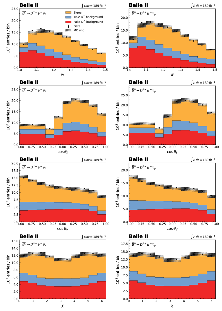
Figure 2: Distributions of observed kinematic variables $w$, $\cos\theta_{\ell}$, $\cos\theta_{V}$, and $\chi$ for ${\kern 1.79993pt\overline{\kern-1.79993ptB}}{}^{0}\to D^{*+}e^{-}\bar{\nu}_{e}$ (left) and ${\kern 1.79993pt\overline{\kern-1.79993ptB}}{}^{0}\to D^{*+}\mu^{-}\bar{\nu}_{\mu}$ (right) candidates reconstructed in data with expected distributions from simulation overlaid. In all panels, simulated samples are shown separately for signal, true $D^{*}$ background, and fake $D^{*}$ background and weighted according to luminosities. The hatched area represents the statistical uncertainty due to the finite size of the simulated samples, and systematic uncertainty arising from the lepton identification, slow pion reconstruction, and tracking efficiency of $K$, $\pi$, and $\ell$.

The signal $B$-meson energy and magnitude of the momentum in the c.m. frame is inferred from the beam energy $E^{\mathrm{c.m.}}_{\mathrm{Beam}}=\sqrt{s}/2$,

$$E^{\mathrm{c.m.}}_{B}=E^{\mathrm{c.m.}}_{\mathrm{Beam}},\quad|\vec{p}^{\,\mathrm{c.m.}}_{B}|=\sqrt{(E^{\mathrm{c.m.}}_{\mathrm{Beam}})^{2}-m^{2}_{B}c^{4}}/c\,.$$ (20)

Here $m_{B}=$5.279\text{\,}\mathrm{G}\mathrm{eV}\mathrm{/}$c^{2}$ is the $B$-meson mass. With this information, we reconstruct the cosine of the angle between the $B$ meson and the $D^{*}\ell$ system (denoted by $Y$) via

$$\cos\theta_{BY}=\frac{2E^{\text{c.m.}}_{B}E^{\text{c.m.}}_{Y}-m^{2}_{B}c^{4}-m^{2}_{Y}c^{4}}{2|\vec{p}^{\,\text{c.m.}}_{B}||\vec{p}^{\,\text{c.m.}}_{Y}|c^{2}},$$ (21)

where $E^{\text{c.m.}}_{Y}$, $|\vec{p}^{\,\text{c.m.}}_{Y}|$, and $m_{Y}$ are the energy, magnitude of momentum, and mass of the reconstructed $D^{*}\ell$ system, respectively. If a $D^{*}\ell$ pair does not originate from a ${\kern 1.79993pt\overline{\kern-1.79993ptB}}{}^{0}\to D^{*+}\ell^{-}\bar{\nu}_{\ell}$ decay, then $|\cos\theta_{BY}|$ can exceed unity. One such possible background are $B\to D^{**}\ell\bar{\nu}_{\ell}$ decays with $D^{**}$ denoting $D_{0}^{*},D_{1}^{\prime},D_{1},D_{2}^{*}$ final states, where missing final state particles may shift $\cos\theta_{BY}$ to large negative values. We retain all candidates in the range $\cos\theta_{BY}\in[-4,2]$ to separate signal decays and background processes.

To reconstruct the recoil parameter $w$ and three helicity angles, the direction of the signal $B$ momentum is needed. It is constrained to lie on a cone around the direction of the $Y$ system with an opening angle $2\theta_{BY}$. To constrain the position of the $B$ momentum on the cone, we exploit the polarization of the $\Upsilon(4S)$, which produces $B$ pairs with an angular distribution of $\sin^{2}\theta$ with respect to the beam axis. This method was introduced by the BaBar experiment in Refs. [39, 40].

Furthermore, we use the tracks and neutral energy depositions (clusters) not associated to the $Y$ system [17]. They originate from the companion $B$ meson, with additional contributions from beam backgrounds. We refer to the collection of these tracks and clusters as the rest of the event (ROE). The ROE can be used to estimate the signal $B$ direction, as it is opposite to the direction of the ROE momentum. However, missing particles, such as neutrinos and $K_{L}^{0}$ mesons, and resolution effects affect the ROE direction. To use both the $B$ meson angular distribution and ROE information, a novel method is developed in this work. We sample 10 $B$-meson directions that are equally spaced on the lateral surface of the cone spanned by $2\theta_{BY}$, and reconstruct $w,\cos\theta_{\ell}$, and $\cos\theta_{V}$ by calculating a weighted average, where weights are written as

$$\alpha_{i}=(1-\hat{p}_{\mathrm{ROE}}\cdot\hat{p}_{B\,i})\sin^{2}\theta_{B\,i}.$$ (22)

Here, $\hat{p}_{\mathrm{ROE}}$ and $\hat{p}_{B\,i}$ denote the unit vector of the ROE and one of sampled $B$ momenta, respectively, and $\theta_{B\,i}$ is the corresponding polar angle of the $B$ meson. However, applying the combined methodology, we observe poor resolution near $\chi=0$ and $2\pi$. Consequently, when reconstructing the angle $\chi$, we identify the direction on the lateral surface of the cone that minimizes the angle with respect to the vector $-\hat{p}_{\mathrm{ROE}}$ as the direction of the $B$ momentum. The biases and resolutions on $w$ and the decay angles are listed in Table 1, where biases are calculated as the medians of differences between reconstructed values and true values, and resolutions are defined as the symmetrical 68% percentiles around the medians of residuals of reconstructed and generated values. The resolution of $\cos\theta_{V}$ is improved by $2\%$ and $7\%$ compared to using only the $B$-meson angular distribution or only ROE information, respectively. Further, the resolutions of the new method for $w$ and $\cos\theta_{\ell}$ are improved by $7\%$ to $12\%$ compared to previous methods [40, 17].

Table 1: Biases and resolutions of the reconstructed recoil parameters and decay angles.

Variable	Bias	Resolution
$w$	$0.001$	$0.04$
$\cos\theta_{\ell}$	$-0.005$	$0.10$
$\cos\theta_{V}$	$0.004$	$0.13$
$\chi$ [rad]	$0.0004$	$0.58$

Figure 2 shows distributions of the reconstructed kinematic variables, where simulated samples are classified as follows

• Signal: the entire decay chain is reconstructed correctly.

• “True $D^{*}$” background: the $D^{*}$ candidate is reconstructed correctly, but the $D^{*}\ell$ system is incorrectly reconstructed due to the misidentification of the lepton candidate or an incorrect combination of $D^{*}$ and $\ell$ candidates. This arises from continuum, $B$-meson background, or signal processes.

• “Fake $D^{*}$” background: the $D^{*}$ candidate is misreconstructed, arising from continuum, $B$-meson background, or signal processes.

We choose a uniform binning for the recoil parameter and the decay angles with ten bins, with the exception of $\cos\theta_{\ell}$, for which we choose eight bins. In general, we observe a fair agreement between simulated samples and experimental data. For the measurement, we determine the signal and background fractions in each bin using a fit to $\cos\theta_{BY}$ and $\Delta M$ distributions.

VI Measurement of partial decay rates

The measurement of partial decay rates in bins of the recoil parameter $w$ and the decay angles is carried out in two steps. First, backgrounds are determined using a likelihood fit and subtracted in each bin independently. The effects of the reconstruction resolution, efficiency, and detector acceptance are then corrected. The statistical correlations between the projected kinematic variables are determined. To validate the fit and unfolding procedure we generated ensembles of simplified simulated experiments. The fits to these ensembles show no biases in central values and no under- or overcoverage of the quoted confidence intervals.

VI.1 Signal extraction

The signal yield in each bin of the kinematic variables is extracted using two-dimensional likelihood fits to the binned $\cos\theta_{BY}$ and $\Delta M$ distributions, as shown in Fig. 3 for the electron and muon final states. The free parameters of the fits are the signal yields, the yields of the true $D^{*}$ background, and the yields of the fake $D^{*}$ background. We use simulated events for the templates. The $\Delta M$ fit separates signal and true $D^{*}$ events, which peak near $0.145$ GeV$/c^{2}$, from the fake $D^{*}$ component.

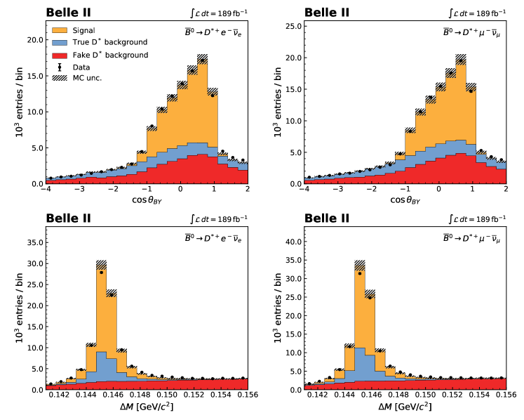
Figure 3: Distributions of reconstructed $\cos\theta_{BY}$ and $\Delta M$ for ${\kern 1.79993pt\overline{\kern-1.79993ptB}}{}^{0}\to D^{*+}e^{-}\bar{\nu}_{e}$ (left) and ${\kern 1.79993pt\overline{\kern-1.79993ptB}}{}^{0}\to D^{*+}\mu^{-}\bar{\nu}_{\mu}$ (right) candidates in data with expectations from simulation overlaid. The simulated samples are weighted according to integrated luminosity. The hatched area represents the uncertainty due to the finite size of the simulated sample, and systematic uncertainties arising from the lepton identification, slow-pion reconstruction, and tracking efficiency of the $K$, $\pi$, and $\ell$.

We choose the following bin granularity with 16 bins in two dimensions: four bins in $\cos\theta_{BY}$ spanning $[-4.0,-2.5,\,-1.0,\,1.0,\,2.0]$ and four equidistant $\Delta M$ bins spanning $[0.141,\,0.156]$ GeV$/c^{2}$.

The expected number of events in bin $i$ of $\cos\theta_{BY}$ and $\Delta M$ is

$$\nu_{i}^{\text{exp}}(\boldsymbol{\nu},\boldsymbol{\theta})=\sum_{k}\,\nu_{k}\,f_{ik}^{\mathrm{MC}}(\boldsymbol{\theta})\,,$$ (23)

where $\nu_{k}$ denotes the yield for the event category $k$, which can be signal, true $D^{*}$ background, and fake $D^{*}$ background. Further, $f_{ik}^{\mathrm{MC}}$ denotes the fraction of events in bin $i$, and is written as

$$f^{\text{MC}}_{ik}(\boldsymbol{\theta})=\frac{p^{\text{MC}}_{ik}(1+\epsilon_{ik}\theta_{ik})}{\sum_{j}p^{\text{MC}}_{jk}(1+\epsilon_{jk}\theta_{jk})}\,,$$ (24)

where $p^{\text{MC}}_{ik}$ is the probability that a $k$ category event is found in bin $i$ as determined from the simulation. This allows the shape of the template to vary according to the nuisance parameter $\theta_{jk}$ and $1\sigma$ deviation $\epsilon_{ik}$ due to the limited size of simulated samples and other systematic sources (see Sec. VII).

The likelihood function for a given bin of the recoil parameter or one of the decay angles is

$$-2\ln{\cal L}(\boldsymbol{\nu},\boldsymbol{\theta})=-2\ln\prod_{i}{\cal P}(\nu_{i}^{\text{obs}},\,\nu_{i}^{\text{exp}})+\boldsymbol{\theta}^{T}C^{-1}_{\theta}\boldsymbol{\theta},$$ (25)

and we minimize it numerically using the iminuit package [41, 42]. Here, $\nu_{i}^{\text{obs}}$ is the number of observed events in data in a given bin and ${\cal P}$ denotes the Poisson distribution. Further, $C_{\theta}$ is the correlation matrix of the nuisance parameters. The resulting signal yields in bins of kinematic variables are provided in Appendix A.

VI.2 Unfolding of fitted yields

The resolution and limited acceptance of the Belle II detector distort the kinematic variables. In order to compare them to the theory expressions of Sec. II, we correct the extracted number of signal events for migrations, efficiencies, and acceptance effects. The migration between observed and true values is expressed as a conditional probability of events being observed in a bin $x$ of the recoil parameter or a decay angle, given that its true value is in bin $y$,

$$\mathcal{M}_{xy}=P(\text{observed in bin}\,\,x|\text{true value in bin}\,\,y)\,.$$ (26)

The matrices summarizing these conditional probabilities for the electron final state are shown in Fig. 4, and those for the muon final state are given in Appendix B. To correct migrations across bins, we apply the singular-value-decomposition unfolding method of Ref. [43]. The method employs a regularization parameter $k$, which dampens statistical fluctuations in the unfolded distributions. To optimize the value of $k$ for each kinematic variable, the simulated signal samples are weighted using the form-factor parameters and their $3\sigma$ uncertainties of Ref. [44]. The bias is defined as the difference of the unfolded spectrum, which is determined with the nominal migration matrix, and the underlying true spectrum. The $k$ values are chosen such that the bias is small, and the ratio of bias and unfolding uncertainty is low and stable. We choose $k=7,6,6$, and $7$ for $w$, $\cos\theta_{\ell}$, $\cos\theta_{V}$, and $\chi$, respectively. These $k$ values provide biases of similar or smaller sizes than unfolding via the inversion of the migration matrices.

The stability of the reported results are further tested by choosing $k$ values equal to the number of bins, resulting in a less constrained curvature regularization, and by using matrix-inversion unfolding. We observe negligible shifts in the form factors and $|V_{cb}|$. Their uncertainties are reported in Sec. VIII.

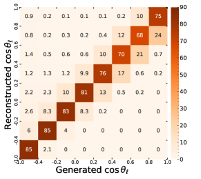
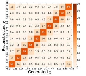
Figure 4: Migration matrices of the reconstructed kinematic variables in the ${\kern 1.79993pt\overline{\kern-1.79993ptB}}{}^{0}\to D^{*+}e^{-}\bar{\nu}_{e}$ decay. The values in the figures are in $10^{-2}$ units.

We determine the partial decay rate in a given kinematic bin $x$ using the unfolded yields $\nu^{\text{unfolded}}_{x}$ via

$$\Delta\Gamma_{x}=\frac{\nu^{\text{unfolded}}_{x}\,\hbar}{\epsilon_{x}\,N_{B^{0}}\,{\cal B}(D^{*+}\to D^{0}\pi^{+})\,{\cal B}(D^{0}\to K^{-}\pi^{+})\,\tau_{B^{0}}},$$ (27)

with $\epsilon_{x}$ denoting the reconstruction efficiency, and $\tau_{B^{0}}$ denoting the $B^{0}$ meson lifetime [3]. The number of produced $B^{0}$ mesons $N_{B^{0}}$ is further discussed in Sec. VII. The resulting partial decay rates and uncertainties are listed in Table 2. The numerical values and full covariance matrices of the measured partial decay rates are available on HEPData [45].

VI.3 Statistical correlations

To analyze the measured partial decay rates simultaneously, we determine the full statistical correlation of the four measured projections. This is done using a bootstrapping approach. We generate $10,000$ replicas of the data sample by resampling with replacement [46]. The total number of sampled events in each replica is varied according to the statistical uncertainty of the full dataset. Each replica is analyzed using the full analysis procedure (background subtraction, unfolding). The resulting statistical correlations are provided in Appendix C. The majority of the bins of different kinematic variables are weakly and positively correlated. Bins of the same variable may exhibit negative or positive correlations due to the unfolding procedure.

Table 2: Measured partial decay rates $\Delta\Gamma$ (in units of $10^{-15}$ GeV/$\hbar$) and average of normalized partial decay rates $\Delta\Gamma/\Gamma$ over ${\kern 1.79993pt\overline{\kern-1.79993ptB}}{}^{0}\to D^{*+}e^{-}\bar{\nu}_{e}$ and ${\kern 1.79993pt\overline{\kern-1.79993ptB}}{}^{0}\to D^{*+}\mu^{-}\bar{\nu}_{\mu}$ decays in bins of kinematic variables. The normalized partial decay rate in the last bin of each projection is excluded in the $|V_{cb}|$ determination to subtract the redundant degrees of freedom. The full (statistical and systematic) uncertainties are provided.

Variable	Bin	$\Delta\Gamma$		$\Delta\Gamma/\Gamma$ average (in %)
		${\kern 1.79993pt\overline{\kern-1.79993ptB}}{}^{0}\to D^{*+}e^{-}\bar{\nu}_{e}$	${\kern 1.79993pt\overline{\kern-1.79993ptB}}{}^{0}\to D^{*+}\mu^{-}\bar{\nu}_{\mu}$	${\kern 1.79993pt\overline{\kern-1.79993ptB}}{}^{0}\to D^{*+}\ell^{-}\bar{\nu}_{\ell}$
$w$	$[1.00,1.05)$	$1.34$ p m 0.10	$1.30$ p m 0.09	$6.19$ p m 0.21
	$[1.05,1.10)$	$2.08$ p m 0.12	$2.11$ p m 0.12	$9.86$ p m 0.22
	$[1.10,1.15)$	$2.40$ p m 0.13	$2.45$ p m 0.13	$11.39$ p m 0.20
	$[1.15,1.20)$	$2.61$ p m 0.14	$2.60$ p m 0.14	$12.18$ p m 0.19
	$[1.20,1.25)$	$2.60$ p m 0.13	$2.60$ p m 0.13	$12.16$ p m 0.17
	$[1.25,1.30)$	$2.49$ p m 0.12	$2.43$ p m 0.12	$11.50$ p m 0.17
	$[1.30,1.35)$	$2.30$ p m 0.11	$2.29$ p m 0.11	$10.72$ p m 0.17
	$[1.35,1.40)$	$2.07$ p m 0.10	$2.07$ p m 0.10	$9.67$ p m 0.18
	$[1.40,1.45)$	$1.83$ p m 0.09	$1.80$ p m 0.09	$8.47$ p m 0.17
	$[1.45,1.51)$	$1.67$ p m 0.09	$1.70$ p m 0.10
$\cos\theta_{\ell}$	$[-1.00,-0.40)$	$3.89$ p m 0.33	$4.10$ p m 0.39	$18.94$ p m 0.79
	$[-0.40,-0.20)$	$2.00$ p m 0.14	$2.07$ p m 0.16	$9.60$ p m 0.27
	$[-0.20,0.00)$	$2.28$ p m 0.12	$2.26$ p m 0.14	$10.63$ p m 0.19
	$[0.00,0.20)$	$2.51$ p m 0.12	$2.56$ p m 0.14	$11.86$ p m 0.24
	$[0.20,0.40)$	$2.73$ p m 0.13	$2.63$ p m 0.13	$12.54$ p m 0.25
	$[0.40,0.60)$	$2.70$ p m 0.13	$2.70$ p m 0.13	$12.68$ p m 0.24
	$[0.60,0.80)$	$2.54$ p m 0.12	$2.57$ p m 0.12	$12.01$ p m 0.24
	$[0.80,1.00)$	$2.52$ p m 0.12	$2.49$ p m 0.12
$\cos\theta_{V}$	$[-1.00,-0.80)$	$2.89$ p m 0.13	$3.02$ p m 0.14	$13.86$ p m 0.27
	$[-0.80,-0.60)$	$2.38$ p m 0.10	$2.32$ p m 0.11	$11.00$ p m 0.18
	$[-0.60,-0.40)$	$1.98$ p m 0.09	$1.93$ p m 0.09	$9.14$ p m 0.13
	$[-0.40,-0.20)$	$1.67$ p m 0.08	$1.65$ p m 0.08	$7.75$ p m 0.11
	$[-0.20,0.00)$	$1.54$ p m 0.08	$1.53$ p m 0.08	$7.18$ p m 0.10
	$[0.00,0.20)$	$1.56$ p m 0.08	$1.58$ p m 0.09	$7.37$ p m 0.11
	$[0.20,0.40)$	$1.73$ p m 0.09	$1.77$ p m 0.10	$8.20$ p m 0.12
	$[0.40,0.60)$	$2.05$ p m 0.11	$2.04$ p m 0.11	$9.59$ p m 0.14
	$[0.60,0.80)$	$2.48$ p m 0.13	$2.42$ p m 0.14	$11.48$ p m 0.17
	$[0.80,1.00)$	$3.07$ p m 0.17	$3.09$ p m 0.18
$\chi$	$[0.00,0.63)$	$1.82$ p m 0.11	$1.85$ p m 0.11	$8.59$ p m 0.21
	$[0.63,1.26)$	$2.20$ p m 0.11	$2.24$ p m 0.12	$10.42$ p m 0.16
	$[1.26,1.88)$	$2.55$ p m 0.13	$2.50$ p m 0.13	$11.82$ p m 0.18
	$[1.88,2.51)$	$2.24$ p m 0.11	$2.24$ p m 0.11	$10.51$ p m 0.16
	$[2.51,3.14)$	$1.85$ p m 0.09	$1.83$ p m 0.10	$8.62$ p m 0.15
	$[3.14,3.77)$	$1.89$ p m 0.10	$1.85$ p m 0.10	$8.75$ p m 0.14
	$[3.77,4.40)$	$2.19$ p m 0.11	$2.21$ p m 0.11	$10.31$ p m 0.16
	$[4.40,5.03)$	$2.47$ p m 0.12	$2.56$ p m 0.13	$11.82$ p m 0.17
	$[5.03,5.65)$	$2.24$ p m 0.11	$2.30$ p m 0.12	$10.67$ p m 0.15
	$[5.65,6.28)$	$1.88$ p m 0.11	$1.75$ p m 0.10

VII Systematic uncertainties

Several systematic uncertainties affect the measured partial rates. They are grouped into uncertainties stemming from the background subtraction and uncertainties affecting the unfolding procedure and the efficiency corrections. A detailed breakdown for each measured partial decay rate is given in Appendix D. The statistical and systematic correlation matrices are given in Appendix C.

VII.1 Background subtraction

The background subtraction is sensitive to the signal and background template shapes in $\cos\theta_{BY}$ and $\Delta M$. To validate the modeling, we reconstruct a sample of same-sign $D^{*+}\ell^{+}$ events, which are free of our signal decay. We observe a fair agreement in the analyzed range of $\cos\theta_{BY}$, but observe some deviations of data from simulation for ${\cos\theta_{BY}>2.5}$. We derive correction factors for both background templates based on $D^{*+}\ell^{+}$ events. We use the high $\Delta M$ region to derive a correction factor for fake $D^{*}$ contributions, and the region near $\Delta M$ of 0.145 GeV/$c^{2}$ to determine a correction for the true $D^{*}$ contribution. The resulting correction factors are in the range [0.85, 1.15]. The full difference between applying and not applying this correction is taken as the systematic uncertainty from background modeling. The systematic uncertainties from the correction factors are treated as uncorrelated. The impact of varying the assumed $B\to D^{**}\ell\bar{\nu}_{\ell}$ background composition is also studied and is found to be negligible.

VII.2 Size of simulated samples

We propagate the statistical uncertainty from the limited size of the simulated sample into the signal and background shapes, migration matrices, and signal efficiencies. For the signal and background shapes, we use nuisance parameters to allow the template shapes in $\cos\theta_{BY}$ and $\Delta M$ to vary within their statistical uncertainties. The uncertainties associated with the finite size of simulated samples are uncorrelated given that they are determined independently bin by bin.

VII.3 Lepton identification

We use bin-wise correction factors as functions of the laboratory momentum and polar angle of the lepton candidates. To determine the uncertainties, we produce 400 replicas of the bin-wise correction factors that fluctuate each factor within its uncorrelated statistical uncertainty and its correlated systematic uncertainty. For each replica, the migration matrices and efficiencies are redetermined and the signal extraction is repeated.

VII.4 Tracking efficiency

We assign a track selection uncertainty of 0.3% per track on kaon, pion, and lepton tracks due to imperfect knowledge of the track-selection efficiency. This uncertainty is determined using a control sample of $e^{+}e^{-}\to\tau^{+}\tau^{-}$ events, and is assumed to be fully correlated between all tracks.

VII.5 Slow-pion reconstruction efficiency

The slow-pion efficiency is determined using $B^{0}\to D^{*-}\pi^{+}$ decays and calculated relative to the tracking efficiency at momenta larger than 200 MeV/$c$ in the laboratory frame. We derive correction factors for three momentum bins spanning $[0.05,0.12,0.16,0.20]\,\mathrm{GeV}/c$. To propagate the impact on the measurement, we produce 400 replicas of the correction weights, taking into account correlations. For each replica, migration matrices and efficiencies are redetermined, and the partial decay rates are remeasured.

VII.6 Number of $B^{0}$ mesons

The number of $B\kern 1.79993pt\overline{\kern-1.79993ptB}$ pairs, $N_{B{\kern 1.25995pt\overline{\kern-1.25995ptB}}}=\left(198\pm 3\right)\times 10^{6}$, is used to determine the total number of $B^{0}$ mesons in the dataset,

$$N_{B^{0}}=2N_{B{\kern 1.25995pt\overline{\kern-1.25995ptB}}}\,(1+f_{+0})^{-1},$$ (28)

with $f_{+0}={\cal B}(\Upsilon(4S)\rightarrow B^{+}B^{-})/{\cal B}(\Upsilon(4S)\rightarrow B^{0}{\kern 1.79993pt\overline{\kern-1.79993ptB}}^{0})=1.065\pm 0.052$ [47]. The uncertainties from both $N_{B{\kern 1.25995pt\overline{\kern-1.25995ptB}}}$ and $f_{+0}$ are propagated into the measured partial decay rates.

VII.7 External inputs

In Eq. (27), the values of ${\cal B}(D^{*+}\to D^{0}\pi^{+})=(67.7\pm 0.5)\%$, ${\cal B}(D^{0}\to K^{-}\pi^{+})=(3.947\pm 0.030)\%$, and the $B^{0}$ lifetime $\tau_{B^{0}}=(1.519\pm 0.004)$ ps are taken from Ref. [3]. The uncertainties from each source are fully correlated across bins of kinematic variables.

VII.8 Dependence of signal model

Simulated ${\kern 1.79993pt\overline{\kern-1.79993ptB}}{}^{0}\to D^{*+}\ell^{-}\bar{\nu}_{\ell}$ samples are used to derive migration matrices and efficiency corrections. This introduces a residual dependence on the assumed model into the results. We use the form-factor parameters and $3\,\sigma$ uncertainties of Ref. [44] to assess the size of this uncertainty. This systematic uncertainty is smaller than the experimental uncertainties and in most bins does not exceed 1%. In the $\cos\theta_{\ell}$ bin of $[-1.0,-0.4]$ it is 4% and comparable to other uncertainties due to the low reconstruction efficiency.

VIII Results

By summing the partial decay rates of all kinematic variables we obtain the total rate. The total decay rates averaged over $w$, $\cos\theta_{\ell}$, $\cos\theta_{V}$, and $\chi$ are converted to branching fractions using the $B^{0}$ lifetime. We find

$${\cal B}({\kern 1.79993pt\overline{\kern-1.79993ptB}}{}^{0}\to D^{*+}e^{-}\bar{\nu}_{e}) =(4.917\pm 0.032\pm 0.216)\%\,,$$ (29)

$${\cal B}({\kern 1.79993pt\overline{\kern-1.79993ptB}}{}^{0}\to D^{*+}\mu^{-}\bar{\nu}_{\mu}) =(4.926\pm 0.032\pm 0.231)\%\,,$$ (30)

where the first and second uncertainties are statistical and systematic, respectively. The average is calculated as

$${\cal B}({\kern 1.79993pt\overline{\kern-1.79993ptB}}{}^{0}\to D^{*+}\ell^{-}\bar{\nu}_{\ell})=(4.922\pm 0.023\pm 0.220)\%\,,$$ (31)

which is compatible with the current world average: $(4.97\pm 0.12)\%$ [3].

As we investigate partial decay rates of the same dataset, the total decay rate is identical on four projections. These are redundant degrees of freedom in the measured partial decay rates within electrons and muons. They are removed before analyzing the observed distributions: we calculate normalized partial decay rates $\Delta\Gamma/\Gamma$ and exclude the last bin of each kinematic variable in the determination of form factors and $|V_{cb}|$.

We average the electron and muon rates and analyze the observed normalized decay rate $\Delta\Gamma^{\text{obs}}_{i}/\Gamma^{\text{obs}}$ and total rate $\Gamma^{\text{obs}}$ by constructing a $\chi^{2}$ function of the form

$$\chi^{2}= \sum_{i,j}^{34}\left(\frac{\Delta\Gamma^{\text{obs}}_{i}}{\Gamma^{\text{obs}}}-\frac{\Delta\Gamma_{i}^{\text{pre}}}{\Gamma^{\text{pre}}}\right)C_{ij}^{-1}\left(\frac{\Delta\Gamma_{j}^{\text{obs}}}{\Gamma^{\text{obs}}}-\frac{\Delta\Gamma^{\text{pre}}_{j}}{\Gamma^{\text{pre}}}\right)$$ (32)

$$\qquad+\frac{(\Gamma^{\text{obs}}-\Gamma^{\text{pre}})^{2}}{\sigma_{\Gamma}^{2}},$$

where $i$ and $j$ denote the indices of the bins in the observables $w$, $\cos\theta_{\ell}$, $\cos\theta_{V}$, and $\chi$, and $\Delta\Gamma_{i}^{\text{pre}}/\Gamma^{\text{pre}}$ and $\Gamma^{\text{pre}}$ are the predicted values expressed as functions of the form-factor parameters and $|V_{cb}|$ [25, 21, 22]. Further, $C$ is the covariance matrix on the normalized rates, and $\sigma_{\Gamma}$ is the uncertainty on the total rate.

The input parameters used in the measurement, e.g., $G_{F}$, $B$-meson mass, and others are summarized in Appendix E. The expansion of BGL form factors must be truncated at a given order. For this we use a nested hypothesis test as proposed in Ref. [48]. We accept a more complex model with an additional expansion parameter over a simpler one if the improvement in $\chi^{2}$ is one unit or greater. We conduct additional testing to ensure that the incorporation of the new expansion parameter does not result in correlations exceeding 95% among any of the fitted parameters. This precaution is taken to prevent overfitting and the emergence of blind directions, i.e., regions within the parameter space where the $\chi^{2}$ is approximately uniform. We identify $n_{a}=1$, $n_{b}=2$, $n_{c}=2$ and in the fits absorb $|V_{cb}|$ into the fitted expansion coefficients $x_{i}=\{a_{i},b_{i},c_{i}\}$,

$$\tilde{x}_{i}=|V_{cb}|\,\eta_{\mathrm{EW}}\,x_{i}\,.$$ (33)

The obtained values and correlations are listed in Table 3 and $|V_{cb}|$ is determined with the relationship

$$|V_{cb}|\eta_{\mathrm{EW}}{\cal F}(1)=\frac{1}{\sqrt{m_{B}m_{D^{*}}}}\left(\frac{|\tilde{b}_{0}|}{P_{f}(0)\phi_{f}(0)}\right)\,.$$ (34)

Using ${\cal F}(1)=0.906\pm 0.013$ [10] and $\eta_{\mathrm{EW}}=1.0066$ [23] we determine

$$|V_{cb}|_{\mathrm{BGL}}=(40.57\pm 0.31\pm 0.95\pm 0.58)\times 10^{-3}.$$ (35)

where the first, second, and third contributions to the uncertainty are statistical, systematic, and from the prediction of ${\cal F}(1)$, respectively. We find a $p$ value of $15$% for the fit.

Fitting the normalized decay rates and the total decay rate with the CLN parametrization we find

$$|V_{cb}|_{\mathrm{CLN}}=(40.13\pm 0.27\pm 0.93\pm 0.58)\times 10^{-3}\,,$$ (36)

with a $p$ value of $16$%. The fitted parameters and correlations are listed in Table 4. Figure 5 compares the measured partial decay rates with the fitted differential decay rates. These spectra have very similar shapes for both parametrizations.

Table 3: Results of the determination of the BGL expansion coefficients and their correlations.

	Value	Correlation				$\chi^{2}$/ndf
$\tilde{a}_{0}\times 10^{3}$	$0.88$ p m 0.05	$1.00$	$0.26$	$-0.28$	$0.19$	39/31
$\tilde{b}_{0}\times 10^{3}$	$0.54$ p m 0.01	$0.26$	$1.00$	$-0.37$	$-0.43$
$\tilde{b}_{1}\times 10^{3}$	$-0.31$ p m 0.30	$-0.28$	$-0.37$	$1.00$	$0.57$
$\tilde{c}_{1}\times 10^{3}$	$-0.04$ p m 0.03	$0.19$	$-0.43$	$0.57$	$1.00$

Table 4: Results of the determination of the CLN parameters, $|V_{cb}|$ and their correlations.

	Value	Correlation				$\chi^{2}$/ndf
$\rho^{2}$	$1.22$ p m 0.05	$1.00$	$0.36$	$-0.81$	$0.29$	39/31
$R_{1}(1)$	$1.14$ p m 0.07	$0.36$	$1.00$	$-0.60$	$-0.10$
$R_{2}(1)$	$0.89$ p m 0.03	$-0.81$	$-0.60$	$1.00$	$-0.08$
$|V_{cb}|\times 10^{3}$	$40.1$ p m 1.1	$0.29$	$-0.10$	$-0.08$	$1.00$

A breakdown of the systematic uncertainties for both fits is provided in Tables 5 and 6 for the BGL and CLN parametrizations respectively. The largest uncertainty on $|V_{cb}|$ originates from the knowledge of the slow-pion reconstruction efficiency followed by the uncertainty on the external input $f_{+0}$.

Table 5: Fractional contributions to the uncertainties of the BGL form factors from a fit of the ${\kern 1.79993pt\overline{\kern-1.79993ptB}}{}^{0}\to D^{*+}\ell^{-}\bar{\nu}_{\ell}$ decay. Because of the absorption of $|V_{cb}|$ into the coefficients (see Eq. (33)), the fitted parameters $\tilde{x}_{i}$ are affected by the uncertainties that only have an impact on the overall normalization.

	$\tilde{a}_{0}$	$\tilde{b}_{0}$	$\tilde{b}_{1}$	$\tilde{c}_{1}$
Statistical	3.7	0.8	$65.1$	$50.8$
Background subtraction	2.1	0.4	$31.3$	$21.8$
Size of simulated samples	1.5	0.3	$26.4$	$20.5$
Lepton ID efficiency	1.6	0.3	$3.4$	$2.8$
Tracking of $K$, $\pi$, $\ell$	0.4	0.4	$0.5$	$0.4$
Slow-pion efficiency	1.6	1.5	$23.8$	$24.7$
$N_{B\kern 1.25995pt\overline{\kern-1.25995ptB}}$	0.8	0.8	$0.8$	$0.8$
$f_{+0}$	1.3	1.3	$1.3$	$1.2$
${\cal B}(D^{*+}\rightarrow D^{0}\pi^{+})$	0.4	0.4	$0.4$	$0.4$
${\cal B}(D^{0}\rightarrow K^{-}\pi^{+})$	0.4	0.4	$0.4$	$0.4$
$B^{0}$ lifetime	0.1	0.1	$0.1$	$0.1$
Signal modeling	2.3	0.5	$52.1$	$35.0$
Total	5.8	2.5	$96.0$	$73.0$

Table 6: Fractional contributions to the uncertainties of the CLN form factors from a fit to the ${\kern 1.79993pt\overline{\kern-1.79993ptB}}{}^{0}\to D^{*+}\ell^{-}\bar{\nu}_{\ell}$ decay. The uncertainties originating from tracking efficiency, the number of $B^{0}$ mesons, the $B^{0}$ lifetime, and the charm branching fractions only affect the overall normalization but do not contribute to the parameters related to the shape.

	$\rho^{2}$	$R_{1}(1)$	$R_{2}(1)$	$|V_{cb}|$
Statistical	3.0	4.1	2.8	0.7
Background subtraction	1.4	2.2	1.2	0.3
Size of simulated samples	1.2	1.7	1.1	0.3
Lepton ID efficiency	0.2	1.6	0.1	0.3
Slow pion efficiency	1.0	0.9	0.8	1.5
Tracking of $K$, $\pi$, $\ell$				0.4
$N_{B\kern 1.25995pt\overline{\kern-1.25995ptB}}$				0.8
$f_{+0}$				1.3
${\cal B}(D^{*+}\rightarrow D^{0}\pi^{+})$				0.4
${\cal B}(D^{0}\rightarrow K^{-}\pi^{+})$				0.4
$B^{0}$ lifetime				0.1
Signal modeling	2.6	2.6	2.0	0.5
Total	4.5	5.9	3.9	2.4

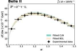
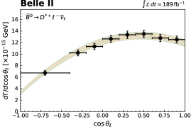
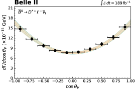
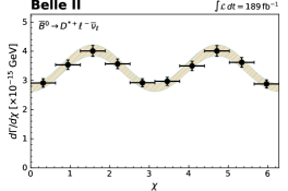
Figure 5: Comparison of the fitted partial decay rates with $1\sigma$ uncertainties in the BGL and CLN parametrizations to the unfolded experimental data (shown as points with error bars). Note that the BGL (hatched) band almost completely overlaps the CLN (solid) band.

VIII.1 Sensitivity to FNAL/MILC lattice results at nonzero recoil

In Ref. [11], the Fermilab lattice and MILC (FNAL/MILC) collaborations published predictions for the ${\kern 1.79993pt\overline{\kern-1.79993ptB}}{}^{0}\to D^{*+}\ell^{-}\bar{\nu}_{\ell}$ form factors at nonzero recoil. We compare our data with these predictions using two scenarios:

• Inclusion of predictions beyond zero recoil for $h_{A_{1}}(w)$ at $w=[1.03,1.10,1.17]$. This scenario allows a comparison with the zero-recoil result when information on the $w$ dependence of $h_{A_{1}}$ is included.

• Inclusion of predictions beyond zero recoil for $h_{A_{1}}(w)$, $R_{1}(w)$, and $R_{2}(w)$ at $w=[1.03,1.10,1.17]$. This scenario includes the full LQCD information.

To include beyond-zero-recoil information, we add to Eq. (32) a term of the form

$$\chi^{2}_{\mathrm{LQCD}}=\sum_{ij}(F_{i}^{\text{LQCD}}-F_{i}^{\text{pre}})C^{-1}_{ij}(F_{j}^{\text{LQCD}}-F_{j}^{\text{pre}})\,.$$ (37)

Here, $F_{i}^{\text{LQCD}}$ denotes the lattice data on $h_{A_{1}}(w)$ or on $h_{A_{1}}(w)$, $R_{1}(w)$, $R_{2}(w)$. The parameter $F_{i}^{\text{pre}}$ represents the corresponding value expressed in terms of form-factor parameters. As we now explicitly include normalization information on the form factors in the fit, we directly fit for the BGL coefficients without absorbing $|V_{cb}|$ and $\eta_{\mathrm{EW}}$.

The fitted results in BGL and CLN parametrizations are summarized in Tables 7 and 8, respectively. The inclusion of beyond-zero-recoil information for $h_{A_{1}}$ results in a small decrease of the central value for $|V_{cb}|$ if we use the BGL form-factor expansion. The CLN fits show a small increase. The inclusion of the full beyond-zero-recoil information shifts $|V_{cb}|$ significantly and the resulting fit shapes in $h_{A_{1}}$, $R_{1}$, and $R_{2}$ disagree with the FNAL/MILC lattice predictions with a poor $p$ value of $0.04\%$. This is consistent with the results of Ref. [49]. The BGL fits of both scenarios are shown in Fig. 6 with the nonzero recoil FNAL/MILC predictions of Ref. [11]. The agreement can be improved if more BGL expansion parameters are included: in Appendix F we repeat the nested hypothesis test to determine the appropriate truncation order when full lattice information is included and find $n_{a}=3$, $n_{b}=1$, $n_{c}=3$. With 6 expansion coefficients we find a $p$ value of 16% because of better agreement of $R_{1}(w)$ and $R_{2}(w)$ at $w=[1.03,1.10,1.17]$.

Table 7: Values of BGL form factors and $|V_{cb}|$ resulting from a fit that includes nonzero recoil lattice information.

	Constraints on $h_{A_{1}}(w)$	Constraints on $h_{A_{1}}(w)$, $R_{1}(w)$, $R_{2}(w)$
$a_{0}\times 10^{3}$	$21.7$ p m 1.3	$25.6$ p m 0.8
$b_{0}\times 10^{3}$	$13.19$ p m 0.24	$13.61$ p m 0.23
$b_{1}\times 10^{3}$	$-6$ p m 6	$2$ p m 6
$c_{1}\times 10^{3}$	$-0.9$ p m 0.7	$-0.0$ p m 0.7
$|V_{cb}|\times 10^{3}$	$40.3$ p m 1.2	$38.3$ p m 1.1
$\chi^{2}$/ndf	39/33	75/39
$p$ value	21%	0.04%

Table 8: Values of CLN form factors and $|V_{cb}|$ resulting from a fit that includes nonzero recoil lattice information.

	Constraints on $h_{A_{1}}(w)$	Constraints on $h_{A_{1}}(w)$, $R_{1}(w)$, $R_{2}(w)$
$h_{A_{1}}(1)$	$0.91$ p m 0.02	$0.94$ p m 0.02
$\rho^{2}$	$1.22$ p m 0.05	$1.21$ p m 0.04
$R_{1}(1)$	$1.14$ p m 0.07	$1.26$ p m 0.04
$R_{2}(1)$	$0.88$ p m 0.03	$0.88$ p m 0.03
$|V_{cb}|\times 10^{3}$	$40.3$ p m 1.2	$38.7$ p m 1.1
$\chi^{2}$/ndf	39/33	70/39
$p$ value	23%	0.2%

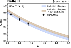
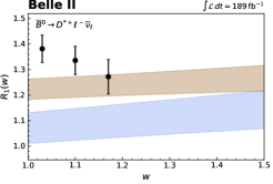
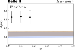
Figure 6: Comparison of the fitted $h_{A_{1}}(w)$, $R_{1}(w)$, and $R_{2}(w)$ for the BGL fits.

VIII.2 Lepton-flavor universality test

We report a value for the ratio of the ${\kern 1.79993pt\overline{\kern-1.79993ptB}}{}^{0}\to D^{*+}e^{-}\bar{\nu}_{e}$ and ${\kern 1.79993pt\overline{\kern-1.79993ptB}}{}^{0}\to D^{*+}\mu^{-}\bar{\nu}_{\mu}$ branching fractions

$$R_{e/\mu}=0.998\pm 0.009\pm 0.020,$$ (38)

where the first contribution to the uncertainty is statistical and the second systematic. The ratio is compatible with the predictions of Refs. [50, 16] (see Table 9 for a summary) assuming LFU and with previous measurements [17, 51]. The fully correlated systematic uncertainties, e.g., the tracking efficiency, the number of $B^{0}$ mesons, and the branching fractions of the $D^{*+}$ and $D^{0}$ decays cancel in the ratio.

From the observed partial decay rates on the $\cos\theta_{\ell}$ projection, we determine the angular asymmetry ${\cal A}_{\mathrm{FB}}$ in the full phase space of $w$,

$${\cal A}_{\mathrm{FB}}=\frac{\int^{1}_{0}\text{d}\cos\theta_{\ell}\text{d}\Gamma/\text{d}\cos\theta_{\ell}-\int^{0}_{-1}\text{d}\cos\theta_{\ell}\text{d}\Gamma/\text{d}\cos\theta_{\ell}}{\int^{1}_{0}\text{d}\cos\theta_{\ell}\text{d}\Gamma/\text{d}\cos\theta_{\ell}+\int^{0}_{-1}\text{d}\cos\theta_{\ell}\text{d}\Gamma/\text{d}\cos\theta_{\ell}}.$$ (39)

With ${\cal A}_{\mathrm{FB}}$ we test LFU using the difference

$$\Delta{\cal A}_{\mathrm{FB}}={\cal A}_{\mathrm{FB}}^{\mu}-{\cal A}_{\mathrm{FB}}^{e}\,.$$ (40)

We find

$${\cal A}_{\mathrm{FB}}^{e} =0.228\pm 0.012\pm 0.018\,,$$ (41)

$${\cal A}_{\mathrm{FB}}^{\mu} =0.211\pm 0.011\pm 0.021\,,$$ (42)

and

$$\Delta{\cal A}_{\mathrm{FB}}=(-17\pm 16\pm 16)\times 10^{-3}\,.$$ (43)

The correlated uncertainties between the ${\kern 1.79993pt\overline{\kern-1.79993ptB}}{}^{0}\to D^{*+}e^{-}\bar{\nu}_{e}$ and ${\kern 1.79993pt\overline{\kern-1.79993ptB}}{}^{0}\to D^{*+}\mu^{-}\bar{\nu}_{\mu}$ decays, e.g., the number of $B^{0}$ mesons, the $B^{0}$ lifetime, and others cancel in $\Delta{\cal A}_{\mathrm{FB}}$. Note that due to the selection requirement on the lepton momentum in the c.m. system, the unfolded yields in the negative $\cos\theta_{\ell}$ region require a large correction based on the SM assumption. Consequently, the measured value of $\Delta{\cal A}_{\mathrm{FB}}$ would change in the presence of non-SM physics, and should only be used to check for consistency with the SM expectation.

To minimize the extrapolation, we also measure ${\cal A}_{\mathrm{FB}}$ in the phase space of $p_{\ell}^{B}>$1.2\text{\,}\mathrm{G}\mathrm{eV}\mathrm{/}$c$, with $p_{\ell}^{B}$ denoting the lepton momentum in the $B$ meson rest frame. We find

$${\cal A}_{\mathrm{FB}}^{e}(p_{\ell}^{B}>$1.2\text{\,}\mathrm{G}\mathrm{eV}\mathrm{/}$c) =0.611\pm 0.006\pm 0.005\,,$$ (44)

$${\cal A}_{\mathrm{FB}}^{\mu}(p_{\ell}^{B}>$1.2\text{\,}\mathrm{G}\mathrm{eV}\mathrm{/}$c) =0.604\pm 0.006\pm 0.008\,,$$ (45)

$$\Delta{\cal A}_{\mathrm{FB}}(p_{\ell}^{B}>$1.2\text{\,}\mathrm{G}\mathrm{eV}\mathrm{/}$c) =\left(-7\pm 9\pm 9\right)\times 10^{-3}\,.$$ (46)

From the observed $\cos\theta_{V}$ distribution, we determine the longitudinal $D^{*}$ polarization fraction $F_{L}$ via

$$\frac{1}{\Gamma}\frac{\text{d}\Gamma}{\text{d}\cos\theta_{V}}=\frac{3}{2}\left(F_{L}\cos^{2}\theta_{V}+\frac{1-F_{L}}{2}\sin^{2}\theta_{V}\right)\,,$$ (47)

and we find

$$F_{L}^{e} =0.520\pm 0.005\pm 0.005\,,$$ (48)

$$F_{L}^{\mu} =0.527\pm 0.005\pm 0.005\,,$$ (49)

and

$$\Delta F_{L}=0.006\pm 0.007\pm 0.005\,,$$ (50)

with $\Delta F_{L}=F_{L}^{\mu}-F_{L}^{e}$. The correlated uncertainties between the ${\kern 1.79993pt\overline{\kern-1.79993ptB}}{}^{0}\to D^{*+}e^{-}\bar{\nu}_{e}$ and ${\kern 1.79993pt\overline{\kern-1.79993ptB}}{}^{0}\to D^{*+}\mu^{-}\bar{\nu}_{\mu}$ decays cancel in $\Delta F_{L}$.

The resulting angular asymmetry and longitudinal polarization for ${\kern 1.79993pt\overline{\kern-1.79993ptB}}{}^{0}\to D^{*+}e^{-}\bar{\nu}_{e}$ and ${\kern 1.79993pt\overline{\kern-1.79993ptB}}{}^{0}\to D^{*+}\mu^{-}\bar{\nu}_{\mu}$ decays and their difference between the $e$ channel and $\mu$ channel agree with the SM predictions of Refs. [16, 50], which are summarized in Table 9. Note that ${\cal A}_{\mathrm{FB}}$ in Ref. [16] is determined from a slightly reduced phase space corresponding to $1.0<w<1.5$. However, the impact of this restriction on the SM expectations is of order $10^{-4}$ [50].

Our values are compatible with the determination of $\Delta{\cal A}_{\mathrm{FB}}$ and $\Delta F_{L}$ of Refs. [16, 17] within 2.3 and 1.2 standard deviations, respectively. Recently Ref. [49] also determined these quantities and we observe good agreement for ${\cal A}_{\mathrm{FB}}$ and $F_{L}$ for electron and muon final states and their differences.

Table 9: Summary of the SM predictions taken from Ref. [50, 16] for LFU tests. Note that the $F_{L}$ in Refs. [50] is only reported with $m_{\ell}=0$ for the light leptons $\ell=e,\mu$.

	Ref. [50]	Ref. [16]
$R_{e/\mu}$	$1.0041\,\pm 0.0001$	$1.0026$ p m 0.0001
${\cal A}^{e}_{\mathrm{FB}}$	$0.244\,\pm 0.004$	$0.204$ p m 0.012
${\cal A}^{\mu}_{\mathrm{FB}}$	$0.239\,\pm 0.004$	$0.198$ p m 0.012
$\Delta{\cal A}_{\mathrm{FB}}\times 10^{3}$	$-5.7\,\pm 0.1$	$-5.33$ p m 0.24
$F_{L}^{e}$	$0.516$ p m 0.003	$0.541$ p m 0.011
$F_{L}^{\mu}$	$0.516$ p m 0.003	$0.542$ p m 0.012
$\Delta F_{L}\times 10^{4}$	$1.2$ p m 0.1	$5.43$ p m 0.36

IX Summary and conclusion

In this paper we present a measurement of partial decay rates of ${\kern 1.79993pt\overline{\kern-1.79993ptB}}{}^{0}\to D^{*+}e^{-}\bar{\nu}_{e}$ and ${\kern 1.79993pt\overline{\kern-1.79993ptB}}{}^{0}\to D^{*+}\mu^{-}\bar{\nu}_{\mu}$ channels using a sample corresponding to $189\,\mathrm{fb}^{-1}$ of Belle II data. We unfold the measured partial decay rates to account for detector and efficiency effects and analyze them to determine form factors and the value of $|V_{cb}|$. Using the BGL parametrization we find

$$|V_{cb}|_{\mathrm{BGL}}=(40.57\pm 0.31\pm 0.95\pm 0.58)\times 10^{-3}\,,$$ (51)

which is in good agreement with the world average of the exclusive approach and the inclusive determination of Refs. [5, 7]. Using the CLN parametrization results in a similar, but lower value,

$$|V_{cb}|_{\mathrm{CLN}}=(40.13\pm 0.27\pm 0.93\pm 0.58)\times 10^{-3}\,.$$ (52)

The obtained $|V_{cb}|$ values of BGL and CLN parametrizations agree with the recent Belle measurement [49]. The slope difference of the form factor near zero recoil is the reason for the small upward shift of the BGL-based $|V_{cb}|$ value in comparison to the CLN result. The slopes of $\mathcal{F}(w)$ at zero recoil are found to be $\mathcal{F}^{\prime}|_{w=1}=-2.03\pm 0.11$ (BGL) and $-1.86\pm 0.08$ (CLN). Both measured values of $|V_{cb}|$ are compatible with the exclusive and inclusive world averages [4, 5] within 1.5 or 1.3 (BGL) and 1.1 or 1.6 (CLN) standard deviations. The precision of the results is limited by the knowledge of the slow-pion efficiency, which can be improved with larger data sets. The current world average of $|V_{cb}|$ is dominated by measurements of ${\kern 1.79993pt\overline{\kern-1.79993ptB}}{}^{0}\to D^{*+}\ell^{-}\bar{\nu}_{\ell}$ decays within the CLN parametrization. Using the values of the CLN parameters taken from Ref. [4], one finds $\mathcal{F}^{\prime}|_{w=1}-1.54\pm 0.05$, which is $\simeq 3$ standard deviations higher than the CLN-based slope reported in this paper.

We also test the impact of including FNAL/MILC lattice predictions at nonzero recoil from Ref. [11] with the same order of BGL expansion in two scenarios: when nonzero recoil information for $h_{A_{1}}$ is included, the resulting value of $|V_{cb}|$ decreases slightly. With the full information on all form factors included, the resulting functional dependence on $h_{A_{1}}$, $R_{1}$ and $R_{2}$ is in tension with the FNAL/MILC lattice predictions, and the BGL fit results in a poor $p$ value of 0.04% if one uses the same number of BGL expansion parameters as for the data only fit. Repeating the fits with more parameters can provide better agreement, but the predicted functional dependence of $R_{2}(w)$ is in tension with the FNAL/MILC LQCD predictions.

We test the electron-muon LFU by determining the ratio of branching fractions. The result

$$R_{e/\mu}=0.998\pm 0.009\pm 0.020,$$ (53)

is in good agreement with unity. To further test LFU, we also measure the forward-backward asymmetry and the $D^{*+}$ polarization, and find $\Delta{\cal A}_{\mathrm{FB}}=(-17\pm 16\pm 16)\times 10^{-3}$ and $\Delta F_{L}=0.006\pm 0.007\pm 0.005$ in good agreement with the SM expectations.

Appendix A SUMMARY OF FITTED YIELDS

The obtained signal yields in bins of kinematic variables are summarized in Table 10.

Table 10: Obtained yields in bins of kinematic variables. The uncertainty is statistical only.

Variable	Bin	${\kern 1.79993pt\overline{\kern-1.79993ptB}}{}^{0}\to D^{*+}e^{-}\bar{\nu}_{e}$	${\kern 1.79993pt\overline{\kern-1.79993ptB}}{}^{0}\to D^{*+}\mu^{-}\bar{\nu}_{\mu}$
$w$	$[1.00,1.05)$	$2004$ p m 84	$2055$ p m 85
	$[1.05,1.10)$	$4519$ p m 120	$4927$ p m 122
	$[1.10,1.15)$	$6252$ p m 126	$6807$ p m 126
	$[1.15,1.20)$	$7433$ p m 127	$7806$ p m 129
	$[1.20,1.25)$	$7636$ p m 125	$8180$ p m 128
	$[1.25,1.30)$	$7326$ p m 121	$7686$ p m 123
	$[1.30,1.35)$	$6531$ p m 112	$7016$ p m 118
	$[1.35,1.40)$	$5615$ p m 106	$6091$ p m 110
	$[1.40,1.45)$	$4699$ p m 100	$4924$ p m 109
	$[1.45,1.51)$	$3352$ p m 99	$3626$ p m 110
$\cos\theta_{\ell}$	$[-1.00,-0.40)$	$1811$ p m 82	$1990$ p m 87
	$[-0.40,-0.20)$	$2136$ p m 81	$2368$ p m 85
	$[-0.20,0.00)$	$5085$ p m 120	$5214$ p m 127
	$[0.00,0.20)$	$8901$ p m 154	$9679$ p m 159
	$[0.20,0.40)$	$10\,163$ p m 145	$10\,056$ p m 146
	$[0.40,0.60)$	$10\,020$ p m 140	$10\,728$ p m 141
	$[0.60,0.80)$	$9286$ p m 132	$10\,312$ p m 139
	$[0.80,1.00)$	$8018$ p m 121	$8872$ p m 129
$\cos\theta_{V}$	$[-1.00,-0.80)$	$7930$ p m 126	$8802$ p m 131
	$[-0.80,-0.60)$	$6963$ p m 122	$7217$ p m 126
	$[-0.60,-0.40)$	$6209$ p m 117	$6481$ p m 121
	$[-0.40,-0.20)$	$5297$ p m 113	$5762$ p m 117
	$[-0.20,0.00)$	$5025$ p m 112	$5321$ p m 114
	$[0.00,0.20)$	$4887$ p m 110	$5194$ p m 112
	$[0.20,0.40)$	$4720$ p m 108	$5235$ p m 110
	$[0.40,0.60)$	$4921$ p m 106	$5234$ p m 109
	$[0.60,0.80)$	$4800$ p m 103	$4935$ p m 107
	$[0.80,1.00)$	$4650$ p m 98	$5038$ p m 104
$\chi$	$[0.00,0.63)$	$4660$ p m 107	$4992$ p m 112
	$[0.63,1.26)$	$5458$ p m 115	$6033$ p m 117
	$[1.26,1.88)$	$6542$ p m 117	$6741$ p m 119
	$[1.88,2.51)$	$5885$ p m 114	$6358$ p m 118
	$[2.51,3.14)$	$5063$ p m 107	$5362$ p m 113
	$[3.14,3.77)$	$5222$ p m 109	$5516$ p m 112
	$[3.77,4.40)$	$5815$ p m 112	$6188$ p m 116
	$[4.40,5.03)$	$6361$ p m 117	$6930$ p m 120
	$[5.03,5.65)$	$5653$ p m 112	$6240$ p m 116
	$[5.65,6.28)$	$4726$ p m 106	$4831$ p m 110

Appendix B MIGRATION MATRICES FOR THE MUON CHANNEL

The migration matrices of $w$, $\cos\theta_{\ell}$, $\cos\theta_{V}$, and $\chi$ for the ${\kern 1.79993pt\overline{\kern-1.79993ptB}}{}^{0}\to D^{*+}\mu^{-}\bar{\nu}_{\mu}$ decay are shown in Fig. 7.

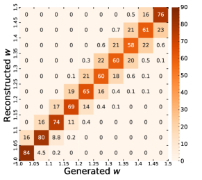
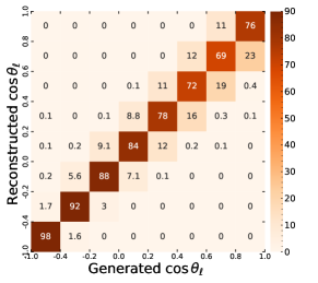
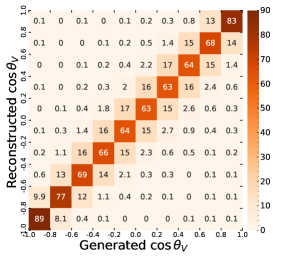
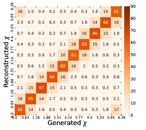
Figure 7: Migration matrices of the reconstructed kinematic variables in the ${\kern 1.79993pt\overline{\kern-1.79993ptB}}{}^{0}\to D^{*+}\mu^{-}\bar{\nu}_{\mu}$ decay. The values in the figures are in units of $10^{-2}$.

Appendix C CORRELATIONS OF PARTIAL DECAY RATE

The statistical and full experimental correlations of the partial decay rates are provided in Figs. 8 and 9, respectively. The full experimental correlations for the average of normalized partial decay rates over ${\kern 1.79993pt\overline{\kern-1.79993ptB}}{}^{0}\to D^{*+}e^{-}\bar{\nu}_{e}$ and ${\kern 1.79993pt\overline{\kern-1.79993ptB}}{}^{0}\to D^{*+}\mu^{-}\bar{\nu}_{\mu}$ decays are given in Fig. 10.

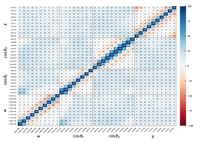
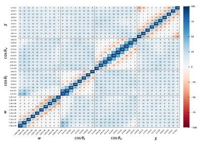
Figure 8: Statistical correlations (in %) of the partial decay rates for the ${\kern 1.79993pt\overline{\kern-1.79993ptB}}{}^{0}\to D^{*+}e^{-}\bar{\nu}_{e}$ (top) and ${\kern 1.79993pt\overline{\kern-1.79993ptB}}{}^{0}\to D^{*+}\mu^{-}\bar{\nu}_{\mu}$ (bottom) decays.

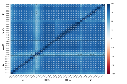
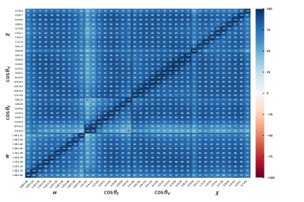
Figure 9: Full experimental (statistical and systematic) correlations (in %) of the partial decay rates for the ${\kern 1.79993pt\overline{\kern-1.79993ptB}}{}^{0}\to D^{*+}e^{-}\bar{\nu}_{e}$ (top) and ${\kern 1.79993pt\overline{\kern-1.79993ptB}}{}^{0}\to D^{*+}\mu^{-}\bar{\nu}_{\mu}$ (bottom) decays.

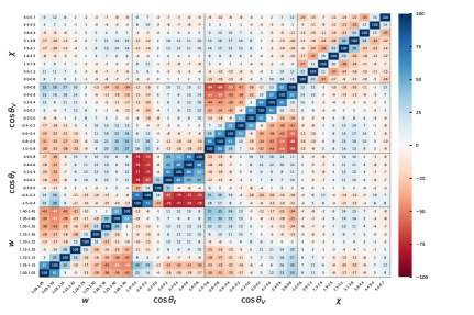
Figure 10: Full experimental (statistical and systematic) correlations (in %) for the average of the normalized partial decay rates. The last bin of each projection is excluded in the determination of $|V_{cb}|$ value, thus it is not shown.

Appendix D STATISTICAL AND SYSTEMATIC UNCERTAINTIES

The uncertainties on the partial decay rates in bins of the $w$, $\cos\theta_{\ell}$, $\cos\theta_{V}$, and $\chi$ projections are classified and summarized in Tables 11 and 12 for the ${\kern 1.79993pt\overline{\kern-1.79993ptB}}{}^{0}\to D^{*+}e^{-}\bar{\nu}_{e}$ and ${\kern 1.79993pt\overline{\kern-1.79993ptB}}{}^{0}\to D^{*+}\mu^{-}\bar{\nu}_{\mu}$ decays, respectively.

Table 11: Fractional uncertainties (in %) of the partial decay rate in each bin for the ${\kern 1.79993pt\overline{\kern-1.79993ptB}}{}^{0}\to D^{*+}e^{-}\bar{\nu}_{e}$ decay.

Variable	Bin	Statistical	Simulated sample size	Signal modeling	Background substraction	Lepton ID efficiency	Slow-pion efficiency	Tracking of $K$, $\pi$, $\ell$	$N_{B\kern 1.25995pt\overline{\kern-1.25995ptB}}$	$f_{+0}$	${\cal B}(D^{*}\rightarrow D\pi)$	${\cal B}(D^{0}\rightarrow K\pi)$	$B^{0}$ lifetime
$w$	$[1.00,1.05)$	3.56	1.48	0.57	2.53	0.65	4.24	0.90	1.52	2.52	0.74	0.76	0.26
	$[1.05,1.10)$	2.25	0.96	0.26	1.72	0.53	3.72	0.90	1.52	2.52	0.74	0.76	0.26
	$[1.10,1.15)$	1.94	0.82	0.55	1.27	0.51	3.34	0.90	1.52	2.52	0.74	0.76	0.26
	$[1.15,1.20)$	1.74	0.74	0.87	1.07	0.45	3.17	0.90	1.52	2.52	0.74	0.76	0.26
	$[1.20,1.25)$	1.72	0.70	0.80	0.98	0.44	2.88	0.90	1.52	2.52	0.74	0.76	0.26
	$[1.25,1.30)$	1.75	0.73	0.70	0.87	0.46	2.73	0.90	1.52	2.52	0.74	0.76	0.26
	$[1.30,1.35)$	1.81	0.84	0.94	0.85	0.45	2.54	0.90	1.52	2.52	0.74	0.76	0.26
	$[1.35,1.40)$	1.94	0.78	1.05	0.83	0.46	2.27	0.90	1.52	2.52	0.74	0.76	0.26
	$[1.40,1.45)$	2.02	0.85	0.92	0.80	0.47	2.10	0.90	1.52	2.52	0.74	0.76	0.26
	$[1.45,1.51)$	2.97	1.36	1.27	0.24	0.51	1.93	0.90	1.52	2.52	0.74	0.76	0.26
$\cos\theta_{\ell}$	$[-1.00,-0.40)$	3.58	1.40	3.96	1.99	0.53	3.57	0.90	1.52	2.52	0.74	0.76	0.26
	$[-0.40,-0.20)$	2.50	1.02	3.08	1.44	0.62	3.27	0.90	1.52	2.52	0.74	0.76	0.26
	$[-0.20,0.00)$	1.95	0.80	1.23	1.18	0.58	2.88	0.90	1.52	2.52	0.74	0.76	0.26
	$[0.00,0.20)$	1.56	0.62	0.66	0.97	0.56	2.59	0.90	1.52	2.52	0.74	0.76	0.26
	$[0.20,0.40)$	1.37	0.61	0.66	0.91	0.62	2.62	0.90	1.52	2.52	0.74	0.76	0.26
	$[0.40,0.60)$	1.37	0.54	0.59	0.93	0.64	2.67	0.90	1.52	2.52	0.74	0.76	0.26
	$[0.60,0.80)$	1.41	0.58	0.76	0.95	0.46	2.73	0.90	1.52	2.52	0.74	0.76	0.26
	$[0.80,1.00)$	1.54	0.68	0.81	1.10	0.30	2.79	0.90	1.52	2.52	0.74	0.76	0.26
$\cos\theta_{V}$	$[-1.00,-0.80)$	1.53	0.70	0.47	0.89	0.53	2.07	0.90	1.52	2.52	0.74	0.76	0.26
	$[-0.80,-0.60)$	1.36	0.58	0.42	0.86	0.52	2.27	0.90	1.52	2.52	0.74	0.76	0.26
	$[-0.60,-0.40)$	1.49	0.66	0.64	1.01	0.50	2.54	0.90	1.52	2.52	0.74	0.76	0.26
	$[-0.40,-0.20)$	1.60	0.68	0.91	1.04	0.47	2.65	0.90	1.52	2.52	0.74	0.76	0.26
	$[-0.20,0.00)$	1.66	0.72	1.24	0.98	0.45	2.85	0.90	1.52	2.52	0.74	0.76	0.26
	$[0.00,0.20)$	1.67	0.71	1.44	0.87	0.45	3.07	0.90	1.52	2.52	0.74	0.76	0.26
	$[0.20,0.40)$	1.66	0.72	1.46	0.77	0.44	3.17	0.90	1.52	2.52	0.74	0.76	0.26
	$[0.40,0.60)$	1.61	0.67	1.38	0.66	0.46	3.40	0.90	1.52	2.52	0.74	0.76	0.26
	$[0.60,0.80)$	1.51	0.63	1.24	0.54	0.45	3.55	0.90	1.52	2.52	0.74	0.76	0.26
	$[0.80,1.00)$	1.98	0.86	1.18	0.12	0.49	3.65	0.90	1.52	2.52	0.74	0.76	0.26
$\chi$	$[0.00,0.63)$	3.02	1.31	1.02	1.87	0.46	3.05	0.90	1.52	2.52	0.74	0.76	0.26
	$[0.63,1.26)$	1.96	0.82	0.87	1.29	0.46	2.89	0.90	1.52	2.52	0.74	0.76	0.26
	$[1.26,1.88)$	1.87	0.81	0.76	1.20	0.46	2.73	0.90	1.52	2.52	0.74	0.76	0.26
	$[1.88,2.51)$	1.96	0.83	0.86	1.22	0.51	2.62	0.90	1.52	2.52	0.74	0.76	0.26
	$[2.51,3.14)$	2.06	0.91	1.10	1.19	0.49	2.44	0.90	1.52	2.52	0.74	0.76	0.26
	$[3.14,3.77)$	2.03	0.85	1.06	1.02	0.51	2.55	0.90	1.52	2.52	0.74	0.76	0.26
	$[3.77,4.40)$	1.98	0.87	0.88	0.88	0.51	2.62	0.90	1.52	2.52	0.74	0.76	0.26
	$[4.40,5.03)$	1.92	0.78	0.67	0.76	0.51	2.77	0.90	1.52	2.52	0.74	0.76	0.26
	$[5.03,5.65)$	1.89	0.80	0.72	0.63	0.46	2.93	0.90	1.52	2.52	0.74	0.76	0.26
	$[5.65,6.28)$	2.89	1.20	1.04	0.51	0.43	2.94	0.90	1.52	2.52	0.74	0.76	0.26

Table 12: Fractional uncertainties (in %) of the partial decay rate in each bin for the ${\kern 1.79993pt\overline{\kern-1.79993ptB}}{}^{0}\to D^{*+}\mu^{-}\bar{\nu}_{\mu}$ decay.

Variable	Bin	Statistical	Simulated sample size	Signal modeling	Background subtraction	Lepton ID efficiency	Slow-pion efficiency	Tracking of $K$, $\pi$, $\ell$	$N_{B\kern 1.25995pt\overline{\kern-1.25995ptB}}$	$f_{+0}$	${\cal B}(D^{*}\rightarrow D\pi)$	${\cal B}(D^{0}\rightarrow K\pi)$	$B^{0}$ lifetime
$w$	$[1.00,1.05)$	3.35	1.32	0.49	1.46	2.00	4.28	0.90	1.52	2.52	0.74	0.76	0.26
	$[1.05,1.10)$	2.04	0.79	0.30	0.97	1.91	3.73	0.90	1.52	2.52	0.74	0.76	0.26
	$[1.10,1.15)$	1.74	0.70	0.69	0.78	1.69	3.33	0.90	1.52	2.52	0.74	0.76	0.26
	$[1.15,1.20)$	1.64	0.72	0.87	0.67	1.62	3.08	0.90	1.52	2.52	0.74	0.76	0.26
	$[1.20,1.25)$	1.61	0.67	0.80	0.61	1.58	2.87	0.90	1.52	2.52	0.74	0.76	0.26
	$[1.25,1.30)$	1.67	0.70	0.84	0.63	1.53	2.64	0.90	1.52	2.52	0.74	0.76	0.26
	$[1.30,1.35)$	1.72	0.68	0.96	0.62	1.57	2.50	0.90	1.52	2.52	0.74	0.76	0.26
	$[1.35,1.40)$	1.85	0.70	1.04	0.59	1.63	2.24	0.90	1.52	2.52	0.74	0.76	0.26
	$[1.40,1.45)$	1.99	0.78	1.00	0.66	1.72	2.06	0.90	1.52	2.52	0.74	0.76	0.26
	$[1.45,1.51)$	2.96	1.15	1.55	0.16	1.81	1.86	0.90	1.52	2.52	0.74	0.76	0.26
$\cos\theta_{\ell}$	$[-1.00,-0.40)$	3.36	1.28	4.20	1.85	3.56	3.76	0.90	1.52	2.52	0.74	0.76	0.26
	$[-0.40,-0.20)$	2.37	0.95	2.99	1.35	3.42	3.14	0.90	1.52	2.52	0.74	0.76	0.26
	$[-0.20,0.00)$	1.88	0.74	1.11	1.11	3.42	2.89	0.90	1.52	2.52	0.74	0.76	0.26
	$[0.00,0.20)$	1.45	0.61	0.59	0.90	2.95	2.59	0.90	1.52	2.52	0.74	0.76	0.26
	$[0.20,0.40)$	1.34	0.52	0.64	0.89	2.02	2.56	0.90	1.52	2.52	0.74	0.76	0.26
	$[0.40,0.60)$	1.27	0.55	0.53	0.88	1.14	2.65	0.90	1.52	2.52	0.74	0.76	0.26
	$[0.60,0.80)$	1.29	0.56	0.68	0.87	0.42	2.67	0.90	1.52	2.52	0.74	0.76	0.26
	$[0.80,1.00)$	1.47	0.59	0.70	1.04	0.15	2.75	0.90	1.52	2.52	0.74	0.76	0.26
$\cos\theta_{V}$	$[-1.00,-0.80)$	1.43	0.64	0.50	0.43	2.04	2.04	0.90	1.52	2.52	0.74	0.76	0.26
	$[-0.80,-0.60)$	1.35	0.55	0.45	0.58	1.77	2.21	0.90	1.52	2.52	0.74	0.76	0.26
	$[-0.60,-0.40)$	1.48	0.62	0.66	0.68	1.56	2.46	0.90	1.52	2.52	0.74	0.76	0.26
	$[-0.40,-0.20)$	1.55	0.64	0.95	0.68	1.46	2.69	0.90	1.52	2.52	0.74	0.76	0.26
	$[-0.20,0.00)$	1.60	0.68	1.23	0.67	1.32	2.89	0.90	1.52	2.52	0.74	0.76	0.26
	$[0.00,0.20)$	1.58	0.66	1.44	0.63	1.34	3.07	0.90	1.52	2.52	0.74	0.76	0.26
	$[0.20,0.40)$	1.56	0.66	1.46	0.57	1.38	3.14	0.90	1.52	2.52	0.74	0.76	0.26
	$[0.40,0.60)$	1.56	0.63	1.40	0.52	1.56	3.30	0.90	1.52	2.52	0.74	0.76	0.26
	$[0.60,0.80)$	1.50	0.61	1.27	0.46	1.82	3.46	0.90	1.52	2.52	0.74	0.76	0.26
	$[0.80,1.00)$	1.94	0.81	1.21	0.07	2.03	3.60	0.90	1.52	2.52	0.74	0.76	0.26
$\chi$	$[0.00,0.63)$	2.88	1.20	1.15	1.02	1.57	2.90	0.90	1.52	2.52	0.74	0.76	0.26
	$[0.63,1.26)$	1.83	0.74	0.82	0.77	1.74	2.91	0.90	1.52	2.52	0.74	0.76	0.26
	$[1.26,1.88)$	1.79	0.77	0.68	0.80	1.78	2.77	0.90	1.52	2.52	0.74	0.76	0.26
	$[1.88,2.51)$	1.84	0.75	0.89	0.77	1.63	2.60	0.90	1.52	2.52	0.74	0.76	0.26
	$[2.51,3.14)$	1.98	0.84	1.11	0.79	1.60	2.50	0.90	1.52	2.52	0.74	0.76	0.26
	$[3.14,3.77)$	1.95	0.79	1.10	0.74	1.56	2.46	0.90	1.52	2.52	0.74	0.76	0.26
	$[3.77,4.40)$	1.86	0.80	0.89	0.65	1.69	2.58	0.90	1.52	2.52	0.74	0.76	0.26
	$[4.40,5.03)$	1.75	0.69	0.74	0.52	1.68	2.73	0.90	1.52	2.52	0.74	0.76	0.26
	$[5.03,5.65)$	1.78	0.72	0.81	0.54	1.70	2.83	0.90	1.52	2.52	0.74	0.76	0.26
	$[5.65,6.28)$	3.00	1.18	0.93	0.32	1.59	2.98	0.90	1.52	2.52	0.74	0.76	0.26

Appendix E INPUT PARAMETERS

In Table 13, we summarize the input parameters used in the BGL parametrization and the determination of partial decay rates.

Table 13: Input parameters of this analysis. All common inputs except the value of $f_{+0}$ are taken from Ref. [3]. The input parameters for the BGL parametrization are taken from Ref. [24].

Common input
$m_{B^{0}}$	$5.27963$ GeV/$c^{2}$
$m_{D^{*}}$	$2.01026$ GeV/$c^{2}$
$\tau_{B^{0}}$	$(1.519\pm 0.004)\times 10^{-12}$ s
${\cal B}(D^{*+}\to D^{0}\pi^{+})$	$0.677\pm 0.005$
${\cal B}(D^{0}\to K^{-}\pi^{+})$	$0.03947\pm 0.00030$
$\eta_{EW}$	$1.0066$
$G_{F}$	$1.1663787\times 10^{-5}$ GeV${}^{-2}(\hbar c)^{3}$
$f_{+0}$	$1.065\pm 0.052$ [47]
BGL input
$n_{I}$	$2.6$
$m_{c}/m_{b}$	$0.33$
$\chi^{T}(+0.33)$	$5.28\times 10^{-4}~{}\mathrm{GeV}^{-2}$
$\chi^{T}(-0.33)$	$3.07\times 10^{-4}~{}\mathrm{GeV}^{-2}$
Vector $B_{c}^{*}$ masses	$6.337$ GeV/$c^{2}$
	$6.899$ GeV/$c^{2}$
	$7.012$ GeV/$c^{2}$
	$7.280$ GeV/$c^{2}$
Axial vector $B_{c}^{*}$ masses	$6.730$ GeV/$c^{2}$
	$6.736$ GeV/$c^{2}$
	$7.135$ GeV/$c^{2}$
	$7.142$ GeV/$c^{2}$

Appendix F NESTED HYPOTHESIS TEST

A nested hypothesis test is carried out to determine the truncation of the BGL form-factor expansion order. It starts from $n_{a}=1$, $n_{b}=1$, $n_{c}=2$ (note that the value of $c_{0}$ is determined from $b_{0}$ parameter via Eq. (16)) to allow at least one degree of freedom from each contributing form factor. We require all correlations between form-factor parameters to be smaller than $95\%$, and $\Delta\chi^{2}=\chi^{2}_{N}-\chi^{2}_{N+1}>1$, when one of the expansion of $g(z)$, $f(z)$, or ${\cal F}_{1}(z)$ is extended to a higher order.

F.1 Test without LQCD input

In this scenario, we only fit experimental data without LQCD predictions. The fitted $|V_{cb}|$ values, minima of the $\chi^{2}$, and numbers of degrees of freedom for various BGL expansion orders are summarized in Table 14. The fitted form-factor parameters with the optimal expansion order $n_{a}=1$, $n_{b}=2$, and $n_{c}=2$ are summarized in the main text in Table 3.

Table 14: Summary of the nested hypothesis test without LQCD input. The $\rho_{\text{max}}$ column records the largest off-diagonal correlation coefficients. The optimal expansion order is highlighted in bold.

$(n_{a},n_{b},n_{c})$	$|V_{cb}|\times 10^{3}$	$\rho_{\text{max}}$	$\chi^{2}$	Ndf	$p$ value
$(1,1,2)$	$40.2$ p m 1.1	$0.43$	$40$	$32$	16%
$(2,1,2)$	$40.1$ p m 1.1	$0.97$	$38.6$	$31$	16%
$(1,2,2)$	$40.6\pm 1.2$	0.57	38.9	31	16%
$(1,1,3)$	$40.1$ p m 1.1	$0.96$	$39.5$	$31$	14%
$(2,2,2)$	$40.3$ p m 1.3	$0.99$	$38.6$	$30$	13%
$(1,3,2)$	$40.0$ p m 1.3	$0.98$	$38$	$30$	15%
$(1,2,3)$	$40.5$ p m 1.2	$0.96$	$38.8$	$30$	13%

F.2 Test with FNAL/MILC lattice results of $h_{A_{1}}$

In this scenario, we fit experimental data and the FNAL/MILC predictions on $h_{A_{1}}(w)$ at $w=[1.03,1.10,1.17]$ simultaneously. The obtained $|V_{cb}|$ values, minima of the $\chi^{2}$, and numbers of degrees of freedom corresponding to various truncations are summarized in Table 15. $n_{a}=1$, $n_{b}=1$, and $n_{c}=2$ is determined as the optimal expansion order. The fitted parameters and their correlations are summarized in Table 16.

Table 15: Summary of the nested hypothesis test when FNAL/MILC predictions on $h_{A_{1}}(w)$ are taken into account.

$(n_{a},n_{b},n_{c})$	$|V_{cb}|\times 10^{3}$	$\rho_{\text{max}}$	$\chi^{2}$	Ndf	$p$ value
$(1,1,2)$	$40.0\pm 1.2$	0.62	40.1	34	22%
$(2,1,2)$	$40.0$ p m 1.2	$0.97$	$38.6$	$33$	23%
$(1,2,2)$	$40.3$ p m 1.2	$0.59$	$39.2$	$33$	21%
$(1,1,3)$	$40.0$ p m 1.2	$0.96$	$39.5$	$33$	20%

Table 16: Fitted parameters and their correlations using the optimal BGL expansion determined with FNAL/MILC constraints on $h_{A_{1}}(w)$.

	Value	Correlation
$|V_{cb}|\times 10^{3}$	$40.0$ p m 1.2	$1.00$	$-0.36$	$-0.62$	$-0.19$
$a_{0}\times 10^{3}$	$21.5$ p m 1.3	$-0.36$	$1.00$	$0.31$	$0.51$
$b_{0}\times 10^{3}$	$13.2$ p m 0.2	$-0.62$	$0.31$	$1.00$	$-0.02$
$c_{1}\times 10^{3}$	$-0.5$ p m 0.6	$-0.19$	$0.51$	$-0.02$	$1.00$

F.3 Test with FNAL/MILC lattice results of $h_{A_{1}}$, $R_{1}$, and $R_{2}$

In the third scenario, we fit experimental data and the FNAL/MILC predictions on $h_{A_{1}}(w)$, $R_{1}(w)$, and $R_{2}(w)$ at $w=[1.03,1.10,1.17]$ simultaneously. The obtained $|V_{cb}|$ values, minima of the $\chi^{2}$, and numbers of degrees of freedom with various truncations are summarized in Table 17. $n_{a}=1$, $n_{b}=3$, and $n_{c}=2$ is determined as the optimal expansion order. The corresponding fitted parameters and their correlations are summarized in Table 18.

Table 17: Summary of the nested hypothesis test when FNAL/MILC predictions on $h_{A_{1}}(w)$, $R_{1}(w)$, and $R_{2}(w)$ are taken into account.

$(n_{a},n_{b},n_{c})$	$|V_{cb}|\times 10^{3}$	$\rho_{\text{max}}$	$\chi^{2}$	Ndf	$p$ value
$(1,1,2)$	$38.3$ p m 1.1	$0.57$	$75.3$	$40$	0.1%
$(2,1,2)$	$39.2$ p m 1.1	$0.59$	$52.4$	$39$	7%
$(1,2,2)$	$38.3$ p m 1.1	$0.61$	$75.2$	$39$	0.1%
$(1,1,3)$	$38.5$ p m 1.1	$0.92$	$73.6$	$39$	0.1%
$(3,1,2)$	$39.5$ p m 1.1	$0.85$	$48.7$	$38$	11%
$(2,2,2)$	$39.2$ p m 1.1	$0.59$	$52.3$	$38$	6%
$(2,1,3)$	$39.4$ p m 1.1	$0.92$	$50.2$	$38$	9%
$(4,1,2)$	$39.4$ p m 1.1	$0.98$	$48.4$	$37$	10%
$(3,2,2)$	$39.3$ p m 1.1	$0.87$	$47.5$	$37$	12%
$(3,1,3)$	$39.7\pm 1.1$	0.92	45.4	37	16%
$(4,2,2)$	$39.2$ p m 1.1	$0.98$	$46.8$	$36$	11%
$(3,3,2)$	$39.3$ p m 1.1	$0.87$	$46.4$	$36$	11%
$(3,2,3)$	$39.6$ p m 1.2	$0.91$	$45.2$	$36$	14%
$(4,3,2)$	$39.3$ p m 1.1	$0.98$	$46$	$35$	10%
$(3,4,2)$	$39.3$ p m 1.1	$0.86$	$46.2$	$35$	10%
$(3,3,3)$	$39.6$ p m 1.2	$0.93$	$45$	$35$	12%
$(4,1,3)$	$39.7$ p m 1.1	$0.98$	$44.1$	$36$	17%
$(3,1,4)$	$39.7$ p m 1.1	$0.91$	$45.3$	$36$	14%
$(2,2,3)$	$39.5$ p m 1.2	$0.91$	$50.1$	$37$	7%
$(2,1,4)$	$39.4$ p m 1.1	$0.91$	$50.1$	$37$	7%
$(1,2,3)$	$38.5$ p m 1.1	$0.91$	$73.6$	$38$	0.1%
$(1,1,4)$	$38.5$ p m 1.1	$0.91$	$73.4$	$38$	0.1%

Table 18: Fitted parameters and their correlations using the optimal BGL expansion determined with FNAL/MILC constraints on $h_{A_{1}}(w)$, $R_{1}(w)$, and $R_{2}(w)$.

	Value	Correlation
$|V_{cb}|\times 10^{3}$	$39.7$ p m 1.1	$1.00$	$-0.16$	$0.03$	$-0.11$	$-0.61$	$-0.16$	$0.11$
$a_{0}\times 10^{3}$	$28.1$ p m 1.0	$-0.16$	$1.00$	$-0.10$	$-0.19$	$0.17$	$0.12$	$-0.03$
$a_{1}\times 10^{3}$	$-44.2$ p m 65.8	$0.03$	$-0.10$	$1.00$	$-0.85$	$-0.04$	$-0.08$	$0.11$
$a_{2}$	$-5.1$ p m 2.4	$-0.11$	$-0.19$	$-0.85$	$1.00$	$0.11$	$0.12$	$-0.12$
$b_{0}\times 10^{3}$	$13.3$ p m 0.2	$-0.61$	$0.17$	$-0.04$	$0.11$	$1.00$	$0.10$	$-0.12$
$c_{1}\times 10^{3}$	$-2.7$ p m 1.3	$-0.16$	$0.12$	$-0.08$	$0.12$	$0.10$	$1.00$	$-0.92$
$c_{2}\times 10^{3}$	$50.8$ p m 27.7	$0.11$	$-0.03$	$0.11$	$-0.12$	$-0.12$	$-0.92$	$1.00$

By comparing results in the three scenarios, we find the inclusion of FNAL/MILC lattice results requires more BGL form-factor parameters to reach an acceptable $\chi^{2}$ value. Using the fitted parameters summarized in Table 16 and Table 18, we compare the $h_{A_{1}}(w)$, $R_{1}(w)$ and $R_{2}(w)$ spectra in Fig. 11. The reoptimized truncation results in a better description of lattice data, while the shapes of partial decay rates remain the same.

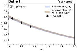
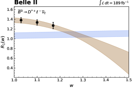
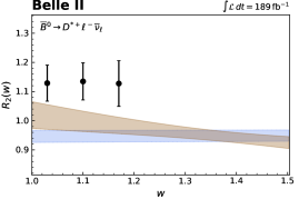
Figure 11: Comparison of the $h_{A_{1}}(w)$, $R_{1}(w)$, and $R_{2}(w)$ spectra with the parameters determined in the nested hypothesis tests when FNAL/MILC lattice predictions are taken into account.