Nucleon electric polarizabilities and nucleon-pion scattering at the physical pion mass

Abstract

We present a lattice QCD calculation of the nucleon electric polarizabilities at the physical pion mass. Our findings reveal the substantial contributions of the $N\pi$ states to these polarizabilities. Without considering these contributions, the lattice results fall significantly below the experimental values, consistent with previous lattice studies. This observation has motivated us to compute both the parity-negative $N\pi$ scattering length and $N\gamma^{*}\to N\pi$ matrix elements using lattice QCD. Our results confirm that the inclusion of dynamic $N\pi$ contributions allows for reliable determination of the polarizabilities from lattice QCD. This methodology lays the groundwork for future lattice QCD investigations into various other polarizabilities.

I Introduction

As building blocks of the visible universe, nucleons play a pivotal role in our pursuit of understanding the internal structure of matter and the unraveling of the mysteries of universe. Being a bound state of quarks and gluons, nucleons exhibit a complex structure that poses significant challenges to understand, particularly at lower energy levels where non-perturbative strong interactions and confinement effects come into play. In the realm of nucleon properties, the electric and magnetic polarizabilities represent crucial fundamental constants akin to the size and shape of the proton. These polarizabilities, denoted as $\alpha_{E}$ and $\beta_{M}$, respectively, offer insights into the distribution of charge and magnetism within nucleons, revealing their response to external electromagnetic fields. Experimental determination of polarizabilities relies on processes such as Compton scattering, wherein external electromagnetic fields polarize the target nucleon or deuteron.

Traditional perturbative QCD techniques are inadequate at low energies, where nonlinearity and strong coupling dominate. Lattice QCD, along with data-driven analysis and effective field theories like chiral perturbation theory ($\chi$PT), offers an avenue to understand nucleon polarizabilities. During the initial stages, lattice QCD calculations of hadron polarizabilities were conducted under the quenched approximation Fiebig et al. (1989); Wilcox (1997, 1998); Christensen et al. (2005); Lee et al. (2006). However, these calculations couldn’t capture the crucial aspect of chiral dynamics, where the nucleon core is surrounded by a pion cloud. Through the decades of dedicated work, lattice QCD can calculate the hadron polarizabilities with full QCD simulations Engelhardt (2007); Detmold et al. (2010); Lujan et al. (2014); Bignell et al. (2018, 2020a); Detmold et al. (2009); Freeman et al. (2014); Bignell et al. (2020b); He et al. (2021); Niyazi et al. (2021); Lee et al. (2023a, b). A recent lattice study focusing on pion electric polarizabilities Feng et al. (2022a) achieved calculations at the physical pion mass ($M_{\pi}$) for the first time, yielding results comparable to predictions from $\chi$PT. However, in the case of nucleon $\alpha_{E}$, lattice results derived from dynamic simulations at heavier-than-physical $M_{\pi}$ Engelhardt (2007); Detmold et al. (2010); Lujan et al. (2014) notably deviate from outcomes obtained through data-driven analysis Schumacher (2019); Pasquini et al. (2019); Krupina et al. (2018); Pasquini et al. (2018); Kossert et al. (2003), $\chi$EFT Lensky et al. (2015); Lensky and McGovern (2014); Myers et al. (2014); McGovern et al. (2013); Bernard et al. (1994), or the PDG average Workman and Others (2022), as depicted in Fig. 1. It’s worth noting that the lattice QCD computation of nucleon electric polarizabilities represents an initial stride toward tackling various other polarizabilities. Hence, comprehending the origins of systematic effects and advancing toward a benchmark calculation holds paramount importance.

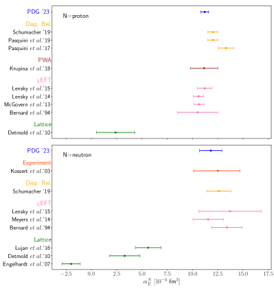
Figure 1: Summary of the electric dipole polarizability for the proton, $\alpha_{E}^{p}$ (upper panel), and the neutron, $\alpha_{E}^{n}$ (lower panel). We utilize a similar figure as presented in Ref. Hagelstein (2020), but with the inclusion of updated PDG data points.

In this work, we extract $\alpha_{E}$ by computing nucleon four-point correlation (4pt) functions at the physical $M_{\pi}$. Upon delving into the detailed contributions from intermediate states in the calculation of these 4pt functions, we discern the pivotal role played by the nucleon-pion ($N\pi$) states. Consequently, we proceed to directly calculate the matrix elements involving $N\pi$, encompassing both isospin $I=\frac{1}{2}$ and $I=\frac{3}{2}$ channels. These matrix elements allows an accurate, indirect determination of the nucleon 4pt function at long distances. The results for $\alpha_{E}^{p}$ and $\alpha_{E}^{n}$ receive substantial contributions from these $N\pi$ states, which would be extremely challenging to obtain through the direct calculation of the 4pt functions alone. By including the $N\pi$ contributions, our final lattice results agree well with the PDG values.

It is noteworthy that $N\pi$ scattering holds intrinsic significance for the investigation of nucleon interactions and the lowest-lying $N\pi$ resonances. While experimental and phenomenological approaches such as the Roy-Steiner equations Ruiz de Elvira et al. (2018); Hoferichter et al. (2023) have yielded a comprehension of the scattering scenario, the direct determination of amplitudes from QCD is constrained by its non-perturbative character at low energies, necessitating input from lattice QCD. Due to the complicated quark field contractions and substantial signal-to-noise challenges, so far, only a limited number of lattice QCD studies address this subject Bulava et al. (2023); Andersen et al. (2018); Lang et al. (2017); Lang and Verduci (2013); Fukugita et al. (1995). Until very recently, the first calculation of $I=\frac{3}{2}$ $N\pi$ scattering length ($a_{0}^{I}$) at the physical $M_{\pi}$ was reported by the ETMC collaboration Alexandrou et al. (2023). In the same vein, we present lattice results for $a_{0}^{I}$ ($I=\frac{1}{2},\frac{3}{2}$) at the physical point, utilizing a different QCD discretization scheme.

II Lattice methodology

We begin with the spin-averaged forward doubly-virtual Compton scattering tensor defined in Euclidean space

$$T^{\mu\nu}(P,Q) = \frac{1}{2}\int d^{4}x\,e^{-iQ\cdot x}\langle N(P)|\mathcal{T}[J^{\mu}(x)J^{\nu}(0)]|N(P)\rangle$$ (1)

$$= \mathcal{K}_{1}^{\mu\nu}T_{1}(Q_{0},Q^{2})+\mathcal{K}_{2}^{\mu\nu}T_{2}(Q_{0},Q^{2})$$

where $P=(iM,\vec{0})$ and $Q=(Q_{0},\vec{Q})$ represent the Euclidean four-momenta of nucleon and photon, respectively, with $M$ denoting the nucleon mass. $J_{\mu,\nu}$ represent the electromagnetic quark currents, while $\mathcal{K}_{1,2}^{\mu\nu}$ signify two conserved Lorentz tensors

$$\mathcal{K}_{1}^{\mu\nu}=\delta^{\mu\nu}Q^{2}-Q^{\mu}Q^{\nu}$$

$$\mathcal{K}_{2}^{\mu\nu}=(P^{\mu}Q^{\nu}+P^{\nu}Q^{\mu})\frac{P\cdot Q}{M^{2}}-\delta^{\mu\nu}\frac{(P\cdot Q)^{2}}{M^{2}}-\frac{P^{\mu}P^{\nu}Q^{2}}{M^{2}}.$$

The scalar function $T_{i}$ can be expressed as a combination of Born ($T_{i}^{B}$) and non-Born ($T_{i}^{NB}$) terms: $T_{i}=T_{i}^{B}+T_{i}^{NB}$. The Born terms, derived from the elastic box and crossed box diagrams, encompass the pole generated by the elastic intermediate states Birse and McGovern (2012). In contrast, the non-Born term remains regular as $Q\to 0$ and, as a result, can be expanded in a Taylor series involving powers of $Q$. The two polarizabilities, $\alpha_{E}$ and $\beta_{M}$, determine the leading terms in the low-energy expansion of $T_{i}^{NB}$

$$T_{1}^{NB}(Q_{0},Q^{2})=\frac{M}{\alpha_{em}}[-\beta_{M}+\mathcal{O}(Q)],$$

$$T_{2}^{NB}(Q_{0},Q^{2})=\frac{M}{\alpha_{em}}[\alpha_{E}+\beta_{M}+\mathcal{O}(Q)].$$ (3)

By conducting a low-$Q$ expansion, we can extract $\alpha_{E}$ from hadronic functions $H^{\mu\nu}(x)$, defined as

$$H^{\mu\nu}(x)=\langle N(P)|\mathcal{T}[J^{\mu}(x)J^{\nu}(0)]|N(P)\rangle.$$ (4)

Specifically, we have three formulae available to calculate $\alpha_{E}$:

$$\alpha_{E}=-\frac{1}{12}\frac{\alpha_{em}}{M}\int d^{4}x\,\vec{x}^{2}\left(H^{00}(x)-H^{00}_{GS}(x)\right)+\alpha_{E}^{r},$$ (5)

$$\alpha_{E}=\frac{1}{4}\frac{\alpha_{em}}{M}\int d^{4}x\,(t+x_{i})^{2}\left(H^{0i}(x)-H^{0i}_{GS}(x)\right)+\alpha_{E}^{r},$$ (6)

and

$$\alpha_{E}=-\frac{1}{12}\frac{\alpha_{em}}{M}\int d^{4}x\,t^{2}\sum_{i}H^{ii}(x)+\alpha_{E}^{r},$$ (7)

with $H^{\mu\nu}_{GS}(x)$ representing the ground-state contribution to $H^{\mu\nu}(x)$, defined as

$$H_{GS}^{\mu\nu}(x)=\langle N(P)|\mathcal{T}[J^{\mu}(x)\hat{P}_{N}J^{\nu}(0)]|N(P)\rangle.$$ (8)

Here $\hat{P}_{N}$ is a projection operator for the nucleon state

$$\hat{P}_{N}=\int\frac{d^{3}\vec{Q}}{(2\pi)^{3}}\frac{1}{2E}|N(\vec{Q})\rangle\langle N(\vec{Q})|,\quad E=\sqrt{M^{2}+\vec{Q}^{2}}.$$ (9)

$\alpha_{E}^{r}$ accounts for residual effects that arise when the pole structure between the Born term and ground-state contribution cancels out. It can be expressed as

$$\alpha_{E}^{r}=\frac{\alpha_{em}}{M}\left(\frac{G_{E}^{2}(0)+\kappa^{2}}{4M^{2}}+\frac{G_{E}(0)\langle r_{E}^{2}\rangle}{3}\right).$$ (10)

where $G_{E}(0)$ represents the electric form factor at zero momentum transfer, with $G_{E}^{p}(0)=1$ and $G_{E}^{n}(0)=0$, respectively. $\kappa$ denotes the nucleon anomalous magnetic moment, and $\langle r_{E}^{2}\rangle$ indicates the squared charge radius.

These position-space formulae (5)-(7) for $\alpha_{E}$ are similar to those invented in Ref. Feng et al. (2022a) for pions. Ref. Wilcox and Lee (2021) has derived a momentum-space formula for $\alpha_{E}$ based on $H^{00}(p)$ at small momentum $p$.

Our position-space formulae, combined with the infinite-volume reconstruction (IVR) method Feng and Jin (2019), allow determination of $\alpha_{E}$ with only exponentially suppressed finite volume errors. The IVR method provides a way to obtain $H^{\mu\nu}_{GS}(x)$ from the lattice calculation of $H^{\mu\nu}(x)$ at sufficiently large time separation. In our calculation, among the three formulae derived, we find $\sum_{i}H^{ii}(x)$ and Eq. (7) provide the best estimate for $\alpha_{E}$ for two reasons. First, $\sum_{i}H^{ii}(x)$ are not enhanced by $\vec{x}^{2}$ near the boundary of the lattice, which leads to smaller finite volume error. Second, it does not receive contribution from the ground state and does not rely on the cancellation between $H^{\mu\nu}(x)$ and $H^{\mu\nu}_{GS}(x)$, which leads to smaller statistical and systematic errors. Consequently, we have opted to rely solely on $\sum_{i}H^{ii}(x)$ and Eq. (7) for the determination of $\alpha_{E}$.

We represent the contribution from $\sum_{i}H^{ii}(x)$ as $\alpha_{E}^{ii}$, and consequently, $\alpha_{E}$ can be expressed as $\alpha_{E}=\alpha_{E}^{ii}+\alpha_{E}^{r}$. The term $\alpha_{E}^{ii}$ encompasses contributions from various intermediate states

$$\alpha_{E}^{ii} = -\frac{1}{12}\frac{\alpha_{em}}{M}\int_{-\infty}^{\infty}dt\,t^{2}\sum_{n}A_{n}e^{-(E_{n}-M)|t|}$$ (11)

$$= -\frac{1}{3}\frac{\alpha_{em}}{M}\sum_{n}\frac{A_{n}}{(E_{n}-M)^{3}},$$

where $A_{n}=\sum_{i}\langle N(\vec{0})|J^{i}|n\rangle\langle n|J^{i}|N(\vec{0})\rangle$ or $-\sum_{i}\langle N\vec{0}|N(\vec{0})\rangle\langle 0|J^{i}|n\rangle\langle n|J^{i}|0\rangle$. For the former, $|n\rangle$ denotes zero-momentum baryonic states with $E_{n}$ representing their energies, while for the latter, $|n\rangle$ denotes the states with zero baryon number, with $E_{n}$ representing their energies plus $M$. These states are normalized as $\langle n^{\prime}|n\rangle=L^{3}\delta_{n^{\prime}n}$. The state with lowest $E_{n}$, $|n=0\rangle$, corresponds to $N\pi$ scattering state near threshold. This state makes the largest contribution to $\alpha_{E}^{ii}$, due to enhancement factor $\frac{1}{(E_{0}-M)^{3}}\approx\frac{1}{M_{\pi}^{3}}$. It’s worth noting that the lattice data of $H^{ii}(t)=\int d^{3}\vec{x}\sum_{i}H^{ii}(t,\vec{x})$ are notably noisy if the time separation $t$ between the two currents exceeds 1 fm, due to the signal-to-noise problem. Therefore, it becomes imperative to introduce a temporal truncation denoted as $t_{0}$ for the integral. Conversely, the integrand $t^{2}e^{-M_{\pi}t}$ exhibits a peak at $t=\frac{2}{M_{\pi}}\approx 2.8$ fm, indicating significant temporal truncation effects. To address this issue, the most straightforward approach is to directly compute the $N\pi$ scattering state near threshold. Once the lattice data for $E_{0}$ and $A_{0}$ become available, it’s possible to separate the hadronic function into ground-state and excited-state components: $H^{ii}(t)=A_{0}e^{-(E_{0}-M)|t|}+H^{ii,es}(t)$. Accordingly, $\alpha_{E}^{ii}$ can also be partitioned into ground-state contribution $\alpha_{E}^{ii,gs}$ and excited-state contribution $\alpha_{E}^{ii,es}$: $\alpha_{E}^{ii}=\alpha_{E}^{ii,gs}+\alpha_{E}^{ii,es}(\infty)$, with

$$\alpha_{E}^{ii,gs}=-\frac{1}{3}\frac{\alpha_{em}}{M}\frac{A_{0}}{\Delta E_{0}^{3}}$$ (12)

and

$$\alpha_{E}^{ii,es}(t_{0}) = -\frac{1}{12}\frac{\alpha_{em}}{M}\int_{-t_{0}}^{t_{0}}dt\,t^{2}H^{ii,es}(t)$$

$$= -\frac{1}{3}\frac{\alpha_{em}}{M}\sum_{n>0}\frac{A_{n}}{\Delta E_{n}^{3}}\left(1-e^{-\Delta E_{n}t_{0}}f(\Delta E_{n},t_{0})\right).$$

Here $\Delta E_{n}=E_{n}-M$ and $f(\Delta E_{n},t_{0})=\frac{1}{2}(\Delta E_{n}t_{0})^{2}+\Delta E_{n}t_{0}+1$. The truncation effects from excited states are anticipated to be considerably less significant compared to $\alpha_{E}^{ii,gs}$. To illustrate, using inputs of $t_{0}=0.75$ fm, $L=4.6$ fm, $M_{\pi}=0.14$ GeV and $M=0.94$ GeV, we observe $\frac{\Delta E_{0}^{3}}{\Delta E_{n}^{3}}e^{-\Delta E_{n}t_{0}}f(\Delta E_{n},t_{0})=5.9\%$, $1.8\%$ and $0.8\%$ for $n=1,2,3$, respectively, where $\Delta E_{n}$ is estimated with the neglect of $N\pi$ rescattering effects.

III Numerical analysis

We utilized two lattice QCD gauge ensembles at the physical $M_{\pi}$, denoted as 24D and 32Dfine, which feature nearly identical spatial size ($L=4.63$ fm and 4.58 fm) but have different lattice spacings ($a^{-1}=1.023(2)$ GeV and 1.378(5) GeV). These ensembles were generated by RBC and UKQCD Collaborations utilizing $2+1$-flavor domain wall fermion Blum et al. (2016). Further ensemble parameters can be found in Ref. Ma et al. (2023). We use 207 configurations for 24D and 69 configurations for 32Dfine. For each configuration, we make use of 1024 point-source and 1024 smeared-point-source propagators at random spatial-temporal locations and subsequently computed three types of correlation functions

$$C_{NJJN}(t_{f},t_{x},t_{y},t_{i})=\langle O_{N}(t_{f})J_{\mu}(t_{x})J_{\nu}(t_{y})O_{N}^{\dagger}(t_{i})\rangle,$$

$$C_{NJN\pi}^{I,I^{\prime}}(t_{f},t,t_{i})=\langle O_{N\pi}^{I}(t_{f})J_{\mu}^{I^{\prime}}(t)O_{N}^{\dagger}(t_{i})\rangle,$$

$$C_{N\pi}^{I}(t_{f},t_{i})=\langle O_{N\pi}^{I}(t_{f}){O_{N\pi}^{I}}^{\dagger}(t_{i})\rangle,$$ (14)

using the random sparsening-field technique Li et al. (2021); Detmold et al. (2021). Here we have performed zero-momentum projection to operators $O_{N}$, $O_{N\pi}$ and $J^{\mu}$. We decompose the electromagnetic current into isovector and isoscalar components: $J_{\mu}=J_{\mu}^{I=1}+J_{\mu}^{I=0}$. The superscripts $I$ and $I^{\prime}$ denote the isospin. We utilized two parameters $\Delta t_{i}$ and $\Delta t_{f}$ to denote the time separation between the nucleon operator and the current insertion. For the correlation function involving two current insertions, $t_{i/f}$ are chosen as $t_{f}=\operatorname{max}\{t_{x},t_{y}\}+\Delta t_{f}$ and $t_{i}=\operatorname{min}\{t_{x},t_{y}\}-\Delta t_{i}$. Local vector current operators were contracted with the renormalization factors quoted from Ref. Feng et al. (2022b). We calculated both connected and disconnected diagrams, discarding only disconnected ones which vanish under the flavor SU(3) limit.

In the left panel of Fig. 2, we present $H^{ii}(t)$ with $\Delta t=\Delta t_{i}+\Delta t_{f}$ fixed at $\sim 0.96$ fm and $0.86$ fm for 24D and 32Dfine, respectively. Clear signals are observed at small $t$. However, as $t$ increases, the signal exhibits an exponential decrease, and noise levels rise rapidly. Consequently, the lattice data already converge towards 0 at about $0.75$ fm. Therefore, we set the temporal truncation $t_{0}$ to $0.75$ fm. According to the current conservation, the low-momentum expansion of the Compton tensor yields $K\equiv\int_{-\infty}^{\infty}dt\,H^{ii}(t)=6\,G_{E}^{2}(0)$ Fu et al. (2022). In the right panel, we present the temporal integral $K(t_{0})\equiv\int_{-t_{0}}^{t_{0}}dt\,H^{ii}(t)$ with $t_{0}\simeq 0.75$ fm as a function of $\Delta t$. As $\Delta t$ increases, the statistical uncertainties escalate significantly. At $\Delta t\simeq 0.91$ fm, we confirm the expected values of $K$, albeit with relatively large uncertainties. These agreements suggest that the temporal truncation effects are not statistically discernible in the computation of $K$. It’s worth noting that, with $\Delta t\simeq 0.91$ fm and $t_{0}\simeq 0.75$ fm, the total source-sink separation amounts to 1.6-1.8 fm. This places substantial demands on the lattice QCD computation of nucleon 4pt functions. The results presented in Fig. 2 are obtained from connected diagrams. As for those arising from disconnected diagrams, we observe that $H^{ii,disc}(t)$ generally tend towards zero but yield uncertainties in $\alpha_{E}^{ii,disc}$ that are 2-3 times larger than the uncertainties of the connected contributions.

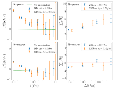
Figure 2: $H^{ii}(t)$ for both proton and neutron. In the left panel, we showcase $H^{ii}(t)$ as a function of $t$, while maintaining $\Delta t\simeq 0.91$ fm. These results are also juxtaposed with contributions from the $N\pi$ ground state. The right panel presents the temporal integral $\int_{-t_{0}}^{t_{0}}dt\,H^{ii}(t)$ as a function of $\Delta t$. At $\Delta t\simeq$ 0.91 fm, the lattice results align with the expected values of $K=6\,G_{E}^{2}(0)$.

To estimate the size of the residual truncation effects from excited states, we define $K^{es}(t_{0})\equiv\int_{-t_{0}}^{t_{0}}dt\,H^{ii,es}(t)$. The temporal truncation effects in $\alpha^{ii,es}_{E}$ can be approximated by

$$\delta_{\mathrm{tr.}}=-\frac{1}{6}\frac{\alpha_{em}}{M}\frac{f(\Delta E_{1},t_{0})}{\Delta E_{1}^{2}}\left[K^{es}(\infty)-K^{es}(t_{0})\right]$$ (15)

with $\Delta E_{1}\approx\sqrt{M^{2}+(\frac{2\pi}{L})^{2}}+\sqrt{M_{\pi}^{2}+(\frac{2\pi}{L})^{2}}-M$. At $t_{0}\simeq 0.75$ fm, we find $\delta_{\mathrm{tr.}}^{p}=-2.0(2.8)$ for 24D and $-2.8(3.7)$ for 32Dfine and $\delta_{\mathrm{tr.}}^{n}=-1.8(2.1)$ for 24D and $-5.3(2.7)$ for 32Dfine. These values are generally consistent with 0, except for one case. Note that $\delta_{\mathrm{tr.}}$ encompasses the entire truncation effect for $|n=1\rangle$ state and the contribution of $|n=1\rangle$ is positive. However, the negative central value suggests that $\delta_{\mathrm{tr.}}$ is mainly due to statistical fluctuations. To be cautious, we use the statistical error of $\delta_{\mathrm{tr.}}$ as an estimate of the systematic uncertainties arising from the temporal truncation, and do not apply the central value of $\delta_{\mathrm{tr.}}$ as a correction to $\alpha_{E}^{ii,es}$.

In the left panel of Fig. 2, the hadronic functions $H^{ii}(t)$ are contrasted with the contributions from the $N\pi$ ground state. These contributions are computed using $C_{NJN\pi}^{I,I^{\prime}}(t_{f},t,t_{i})$ and $C_{N\pi}^{I}(t_{f},t_{i})$. To begin, we calculate the energy shift $\delta E_{I}$ for the $N\pi$ scattering states in the isospin $I=\frac{1}{2}$ and $\frac{3}{2}$ channels by defining the ratio

$$R^{I}(t)=\frac{C_{N\pi}^{I}(t_{f},t_{i})}{C_{N}(t_{f},t_{i})C_{\pi}(t_{f},t_{i})}\approx A_{I}(1-\delta E_{I}\,t),$$ (16)

where $t=t_{f}-t_{i}$ and $\delta E_{I}=E_{I}-M-M_{\pi}$ with $E_{I}$ representing the energy for the $N\pi$ state near the threshold. $C_{N}$ and $C_{\pi}$ represent the nucleon and pion two-point correlation functions. In Fig. 3, we present the $t$ dependence of $R_{I}(t)$ along with a correlated fit to a linear function of $t$. Via this fit, we extract $\delta E_{I}$ for both isospin channels. Remarkably, as the lattice sizes of 24D and 32Dfine are nearly identical (with only a 1% difference), the two ensembles yield highly consistent results for $\delta E_{I}$, despite their differing lattice spacings. In a prior study of $\pi\pi$ scattering using the same two ensembles Blum et al. (2023), $\delta E_{I}$ for $I=0$ and $2$ exhibited only a 1% difference between different ensembles. This is not surprising, as lattice artifacts are proportionally related to the weak interaction in $\pi\pi$ and $N\pi$ scattering. Furthermore, $\chi$PT informs us that interactions involving $\pi$ at the threshold vanish in the chiral limit. Therefore, in the $N\pi$ system, we believe that the difference in $\delta E_{I}$ between 24D and 32Dfine is mainly attributable to the statistical fluctuations rather than lattice artifacts. Instead of conducting the continuum extrapolation, we opt for a combined fit using both ensembles.

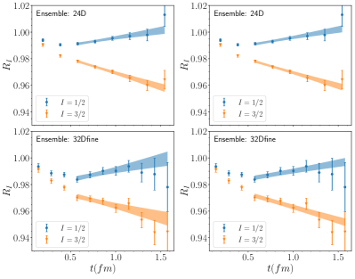
Figure 3: $R_{I}(t)$ for $I=\frac{1}{2}$ and $\frac{3}{2}$ as a function of $t$. The 24D and 32Dfine results are depicted in the upper and lower panels, respectively. In the left panel, we perform the correlated fits to the linear form individually, while in the right panel, we conduct a combined fit using data from both the 24D and 32Dfine ensembles.

Next, we compute three types of matrix elements ${{}_{I}}\langle N\pi|J_{i}|N\rangle$: ${{}_{\frac{3}{2}}}\langle N\pi|J_{i}^{I=1}|N\rangle$, ${}_{\frac{1}{2}}\langle N\pi|J_{i}^{I=1}|N\rangle$ and ${{}_{\frac{1}{2}}}\langle N\pi|J_{i}^{I=0}|N\rangle$, with both initial and final states at rest. These matrix elements are normalized as $\langle N|N\rangle=2ML^{3}$ and ${{}_{I}}\langle N\pi|N\pi\rangle_{I}=L^{3}$. We use the ratio

$$R^{I,I^{\prime}}(t,T_{s}) = \frac{C_{NJN\pi}^{I,I^{\prime}}(t_{f},t,t_{i})}{C_{N\pi}(t_{f},t_{i})}$$ (17)

$$\times \sqrt{\frac{C_{N}^{I}(t_{f},t)C_{N\pi}^{I}(t,t_{i})C_{N\pi}^{I}(t_{f},t_{i})}{C_{N\pi}^{I}(t_{f},t)C_{N}(t,t_{i})C_{N}(t_{f},t_{i})}}$$

with $T_{s}=t_{f}-t_{i}$ to build the summed insertion Maiani et al. (1987); Gusken et al. (1989); Bulava et al. (2012); Capitani et al. (2012)

$$S^{I,I^{\prime}}(T_{s}) = \sum_{t=t_{i}+a}^{t_{f}-a}R^{I,I^{\prime}}(t,T_{s})$$ (18)

$$\xrightarrow[]{T_{s}\to\infty} c_{0}+\frac{1}{\sqrt{2M}}{{}_{I}}\langle N\pi|J_{i}^{I^{\prime}}|N\rangle\cdot T_{s}+\cdots,$$

where the dots stand for excited-state contamination that are exponentially suppressed as $T_{s}$ increases. By fitting $S^{I,I^{\prime}}(T_{s})$ to a linear form of $T_{s}$, we extract the dimensionless quantity $\frac{1}{\sqrt{2M}}{{}_{I}}\langle N\pi|J_{i}^{I^{\prime}}|N\rangle$, as depicted in Fig. 4.

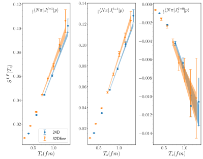
Figure 4: The summed insertion $S^{I,I^{\prime}}(T_{s})$ as a function of $T_{s}$. The three panels showcase $S^{I,I^{\prime}}(T_{s})$ for $\{I,I^{\prime}\}=\{\frac{3}{2},1\}$, $\{\frac{1}{2},1\}$ and $\{\frac{1}{2},0\}$, respectively.

IV Results and conclusion

Through the linear fit shown in Fig. 3, we determine $\delta E_{I}$ for $I=\frac{1}{2}$ and $\frac{3}{2}$ and extract $a_{0}^{I}$ (multiplied with $M_{\pi}$ and denoted as $M_{\pi}a_{0}^{I}$) by incorporating $\delta E_{I}$ into Lüscher formula Luscher (1986); Torok et al. (2010). As depicted in Table 1, the results obtained from individual ensembles agree are in agreement with each other and also consistent with those from the combined fit. When extracting $M_{\pi}a_{0}^{I}$, we note slight variations in the parameters for $M$, $M_{\pi}$ and $L$, resulting in a negligible deviation of $0.002$ compared to the statistical error. We observe that our lattice results for $M_{\pi}a_{0}^{\frac{3}{2}}$ aligns well with the recent lattice results at the physical $M_{\pi}$, specifically $M_{\pi}a_{0}^{\frac{3}{2}}=-0.131(26)$, as reported by the ETMC collaboration Alexandrou et al. (2023). However, our results exhibit deviations of 1-3$\sigma$ when compared to the data-driven analysis: $M_{\pi}a_{0}^{\frac{1}{2}}=0.170(2)$ and $M_{\pi}a_{0}^{\frac{1}{2}}=-0.087(2)$ Hoferichter et al. (2023). It’s worth noting that the data-driven analysis relies on the charged $M_{\pi}$, while lattice-QCD calculations employ the $M_{\pi}$ under the isospin limit. The inclusion of isospin-breaking effects helps to alleviate the tension observed in the $N\pi$ $\sigma$-term between lattice calculations and data-driven analysis Hoferichter et al. (2023). Given the close connection between $N\pi$ scattering and the $\sigma$-term, it is important to investigate whether isospin-breaking effects may also significantly impact $a_{0}^{I}$ in future studies. Moreover, utilizing a broader range of interpolating operators in a variational analysis will be beneficial.

	Ensemble	24D	32Dfine	Combined fit
	$\chi^{2}/\mathrm{dof}$	0.52	0.64	0.57
$I=\frac{1}{2}$	$\delta E_{I}$ [MeV]	$-2.18(70)$	$-3.0(1.2)$	$-2.38(61)$
	$M_{\pi}a_{0}^{I}$	0.086(29)	0.118(53)	0.093(25)(2)
	$\chi^{2}/\mathrm{dof}$	0.32	0.85	0.76
$I=\frac{3}{2}$	$\delta E_{I}$ [MeV]	$4.17(63)$	$3.4(1.1)$	$3.97(54)$
	$M_{\pi}a_{0}^{I}$	$-0.135(18)$	$-0.111(34)$	$-0.128(15)(2)$

Table 1: Fitting results for the energy shifts ($\delta E_{I}$) and scattering lengths ($M_{\pi}a_{0}^{I}$) in both $I=\frac{1}{2}$ and $\frac{3}{2}$ channels, obtained from individual ensembles as well as the combined analysis.

The final results of $\alpha_{E}^{ii,gs}$, $\alpha_{E}^{ii,es}$, $\alpha_{E}^{ii,disc}$, $\alpha_{E}^{r}$ and total contribution $\alpha_{E}$ are summarized in Table 2. For $\alpha_{E}$, the first uncertainty reflects statistical considerations, while the second accounts for the residual temporal truncation effects. These results are in good agreement with the PDG values Workman and Others (2022). Notably, the $N\pi$ ground state amounts for about $60\%$ of $\alpha_{E}^{p}$ and $80\%$ of $\alpha_{E}^{n}$. This not only elucidates why previous lattice results were significantly lower but also underscores the substantial challenges in lattice QCD calculations of polarizabilities. Presently, we report relatively large uncertainties due to temporal truncation. It is advisable to mitigate these uncertainties by investigating additional low-lying $N\pi$ contributions in future studies.

		24D	32Dfine	PDG
	$\alpha_{E}^{ii,gs}$	6.51(45)	8.03(85)	-
	$\alpha_{E}^{ii,es}$	$-0.92(53)$	$-0.94(62)$	-
proton	$\alpha_{E}^{ii,disc}$	$1.4(1.2)$	$0.4(2.0)$
	$\alpha_{E}^{r}$	4.333(3)	4.333(3)	-
	$\alpha_{E}$	$11.3(1.4)(2.8)$	$11.8(2.3)(3.7)$	11.2(4)
	$\alpha_{E}^{ii,gs}$	8.93(57)	10.5(1.0)	-
	$\alpha_{E}^{ii,es}$	$0.18(40)$	$0.54(47)$
neutron	$\alpha_{E}^{ii,disc}$	$1.4(1.2)$	$0.4(2.0)$
	$\alpha_{E}^{r}$	0.618(1)	0.618(1)	-
	$\alpha_{E}$	$11.1(1.4)(2.1)$	$12.0(2.3)(2.7)$	11.8(1.1)

Table 2: Proton and neutron polarizabilities determined in this work. We list the results of $\alpha_{E}^{ii,gs}$, $\alpha_{E}^{ii,es}$, $\alpha_{E}^{ii,disc}$, $\alpha_{E}^{r}$ and $\alpha_{E}$ as well as the PDG values in units of $10^{-4}$ fm³.

V Supplementary Material

V.1 Useful formulae to extract $\alpha_{E}$ and $\beta_{M}$

It is not unique to determine $\alpha_{E}$ and $\beta_{M}$ using the hadronic functions $H^{\mu\nu}(x)$ as inputs. With $P=(iM,\vec{0})$, $Q=(Q_{0},\vec{Q})$ as inputs, we have

$$\mathcal{K}_{1}^{00}=\mathcal{K}_{2}^{00}=\vec{Q}^{2},\quad\mathcal{K}_{1}^{0i}=\mathcal{K}_{2}^{0i}=-Q_{0}Q_{i},$$

$$\sum_{i}\mathcal{K}_{1}^{ii}=3Q_{0}^{2}+2\vec{Q}^{2},\quad\sum_{i}\mathcal{K}_{2}^{ii}=3Q_{0}^{2},$$

$$\mathcal{K}_{1}^{ij}=-Q_{i}Q_{j},\quad\mathcal{K}_{2}^{ij}=0.$$ (S 1)

The Born terms are given as follows Birse and McGovern (2012)

$$T_{1}^{B}(Q_{0},Q^{2}) = -\frac{Q^{2}(2F_{1}F_{2}+F_{2}^{2})+Q_{0}^{2}F_{2}^{2}}{Q^{4}+4M^{2}Q_{0}^{2}}$$

$$T_{2}^{B}(Q_{0},Q^{2}) = \frac{Q^{2}F_{2}^{2}+4M^{2}F_{1}^{2}}{Q^{4}+4M^{2}Q_{0}^{2}}.$$ (S 2)

Here the factor $1/(Q^{4}+4M^{2}Q_{0}^{2})=1/[(s-M^{2})(u-M^{2})]$ emerges from the poles present in the $s$- and $u$-channels with $s=-(P+Q)^{2}$ and $u=-(P-Q)^{2}$. In Eq. (V.1), $F_{1,2}(Q^{2})$ refer to the nucleon’s Dirac and Pauli form factors, respectively.

The low-$Q$ expansion of the Compton tensors is expressed as

$$T^{00} = \vec{Q}^{2}\left(T_{1}^{B}+T_{2}^{B}+\frac{M}{\alpha_{em}}\alpha_{E}\right)+\mathcal{O}(Q^{3}),$$

$$T^{0i} = -Q_{0}Q_{i}\left(T_{1}^{B}+T_{2}^{B}+\frac{M}{\alpha_{em}}\alpha_{E}\right)+\mathcal{O}(Q^{3}),$$

$$T^{ii} = Q_{0}^{2}\left(T_{1}^{B}+T_{2}^{B}+\frac{M}{\alpha_{em}}\alpha_{E}\right)$$

$$+ (\vec{Q}^{2}-Q_{i}^{2})\left(T_{1}^{B}-\frac{M}{\alpha_{em}}\beta_{M}\right)+\mathcal{O}(Q^{3})$$

$$T^{ij} = -Q_{i}Q_{j}\left(T_{1}^{B}-\frac{M}{\alpha_{em}}\beta_{M}\right)+\mathcal{O}(Q^{3})$$ (S 3)

Consequently, we have the flexibility to use either $H^{00}$, $H^{0i}$ or $\sum_{i}H^{ii}$ to extract $\alpha_{E}$ and either $\sum_{i}H^{ii}$ or $H^{ij}$ to extract $\beta_{M}$.

In the extraction of $\alpha_{E}$, as $T_{1}^{B}$ and $T_{2}^{B}$ are consistently combined, we define their combination as $T^{B}$:

$$T^{B}\equiv T_{1}^{B}+T_{2}^{B}=\frac{4M^{2}G_{E}^{2}(Q^{2})}{Q^{4}+4M^{2}Q_{0}^{2}}-\frac{F_{2}^{2}(Q^{2})}{4M^{2}}.$$ (S 4)

Here we have introduced the electric and magnetic form factors

$$G_{E}(Q^{2}) = F_{1}(Q^{2})-\frac{Q^{2}}{4M^{2}}F_{2}(Q^{2}),$$

$$G_{M}(Q^{2}) = F_{1}(Q^{2})+F_{2}(Q^{2}).$$ (S 5)

The low-$Q^{2}$ expansion of $G_{E/M}$ yields

$$G_{E}(Q^{2}) = G_{E}(0)-\frac{\langle r_{E}^{2}\rangle}{6}Q^{2}+\frac{\langle r_{E}^{4}\rangle}{120}Q^{4}+\mathcal{O}(Q^{6}),$$

$$G_{M}(Q^{2}) = G_{M}(0)+\mathcal{O}(Q^{2})=G_{E}(0)+\kappa+\mathcal{O}(Q^{2}),$$

where $\langle r_{E}^{2}\rangle$ and $\langle r_{E}^{4}\rangle$ represent squared and quartic charge radius. $\kappa$ stands for the anomalous magnetic moment of the nucleon.

It’s important to note that $T^{B}$ contains the pole structure, which should be compensated by the ground-state contributions to $H^{\mu\nu}(t,\vec{x})$. These contributions, denoted as $H_{GS}^{\mu\nu}$, are given by

$$H_{GS}^{\mu\nu}(t,\vec{x})\Big{|}_{t>0} = \int\frac{d^{3}\vec{Q}}{(2\pi)^{3}}\,\frac{e^{-(E-M)t}e^{i\vec{Q}\cdot\vec{x}}}{2E}$$

$$\langle N(\vec{0})|J^{\mu}(0)|N(\vec{Q})\rangle\langle N(\vec{Q})|J^{\nu}(0)]|N(\vec{0})\rangle,$$

$$H_{GS}^{\mu\nu}(t,\vec{x})\Big{|}_{t<0} = H_{GS}^{\nu\mu}(-t,-\vec{x}),$$ (S 7)

where the matrix elements’ product is described as

$$\mathcal{M}^{\mu\nu} \equiv \langle N(\vec{0})|J^{\mu}(0)|N(\vec{Q})\rangle\langle N(\vec{Q})|J^{\nu}(0)|N(\vec{0})\rangle$$

$$= \begin{cases}2M(E+M)G_{E}^{2}(Q_{on}^{2}),&\mu=\nu=0,\\ -2iMQ_{i}G_{E}^{2}(Q_{on}^{2}),&\mu,\nu=0,i,\\ -Q_{on}^{2}\left[\frac{Q_{i}^{2}}{\vec{Q}^{2}}G_{E}^{2}+\left(1-\frac{Q_{i}^{2}}{\vec{Q}^{2}}\right)G_{M}^{2}\right],&\mu=\nu=i,\\ Q_{on}^{2}\frac{Q_{i}Q_{j}}{\vec{Q}^{2}}[G_{M}^{2}(Q_{on}^{2})-G_{E}^{2}(Q_{on}^{2})],&\mu=i,\nu=j.\end{cases}$$

The squared momentum $Q_{on}^{2}$ results from the momentum transfer between two on-shell states and is represented as

$$Q_{on}^{2}=(iE-iM)^{2}+\vec{Q}^{2}=2M(E-M).$$ (S 9)

Putting the matrix elements’ product into the Compton tensor, we arrive at

$$T_{GS}^{\mu\nu}=\mathcal{M}^{\mu\nu}\frac{M}{E}\times\begin{cases}\frac{Q_{on}^{2}}{Q_{on}^{4}+4M^{2}Q_{0}^{2}},&\vec{Q}\neq 0,\\ \frac{\sin(Q_{0}t_{0})}{2MQ_{0}},&\vec{Q}=0,\end{cases}$$ (S 10)

for $\mu=\nu=0$, $\mu=\nu=i$ and $\mu=i,\nu=j$, and

$$T_{GS}^{\mu\nu}=\mathcal{M}^{\mu\nu}\frac{M}{E}\times\begin{cases}\frac{-i2MQ_{0}}{Q_{on}^{4}+4M^{2}Q_{0}^{2}},&\vec{Q}\neq 0,\\ \frac{-i(1-\cos(Q_{0}t_{0}))}{2MQ_{0}},&\vec{Q}=0,\\ \end{cases}$$ (S 11)

for $\mu,\nu=0,i$. In the case of $\vec{Q}=0$, a temporal truncation $t_{0}$ has been introduced.

By combining Eqs. (V.1), (S 4) and (S 10) and considering the momentum assignments, $Q=(0,\vec{\xi})$ for $T^{00}$, $(\xi,0,0,\xi)$ for $T^{03}$ and $(\xi,\vec{0})$ for $T^{ii}$, we can derive three formulae for determining $\alpha_{E}$, specifically

$$\alpha_{E} = \lim_{\vec{Q}^{2}=\xi^{2}\to 0}\frac{\alpha_{em}}{M}\left(\frac{T^{00}-T_{GS}^{00}}{\vec{Q}^{2}}-\frac{\vec{Q}^{2}T^{B}-T_{GS}^{00}}{\vec{Q}^{2}}\right)$$

$$= -\frac{1}{12}\frac{\alpha_{em}}{M}\int d^{4}x\,\vec{x}^{2}\left(H^{00}(x)-H^{00}_{GS}(x)\right)+\alpha_{E}^{r},$$

$$\alpha_{E} = \lim_{Q_{0}^{2}=Q_{3}^{2}=\xi^{2}\to 0}\frac{\alpha_{em}}{M}\left(\frac{T^{03}-T_{GS}^{03}}{-Q_{0}Q_{3}}-\frac{-Q_{0}Q_{3}T^{B}-T_{GS}^{03}}{-Q_{0}Q_{3}}\right)$$

$$= \frac{1}{4}\frac{\alpha_{em}}{M}\int d^{4}x\,(t+z)^{2}\left(H^{03}(x)-H^{03}_{GS}(x)\right)+\alpha_{E}^{r},$$

and

$$\alpha_{E} = \lim_{Q_{0}^{2}=\xi^{2}\to 0}\frac{\alpha_{em}}{M}\left(\frac{T^{ii}}{Q_{0}^{2}}-T^{B}\right)$$ (S 14)

$$= -\frac{1}{4}\frac{\alpha_{em}}{M}\int d^{4}x\,t^{2}H^{ii}(x)+\alpha_{E}^{r},$$

with

$$\alpha_{E}^{r}=\frac{\alpha_{em}}{M}\left(\frac{G_{E}^{2}(0)+\kappa^{2}}{4M^{2}}+\frac{G_{E}(0)\langle r_{E}^{2}\rangle}{3}\right).$$ (S 15)

To calculate $\beta_{M}$, we can use $Q=(0,\xi,0,0)$ for $T^{33}$ or $Q=(0,0,\xi,\xi)$ for $T^{23}$ and obtain two formulae

$$\beta_{M} = \lim_{\vec{Q}^{2}=\xi^{2}\to 0}-\frac{\alpha_{em}}{M}\left(\frac{T^{33}(\vec{\xi})-T_{GS}^{33}(\vec{\xi})-T_{ES}^{33}(\vec{0})}{Q_{1}^{2}}\right.$$ (S 17)

$$\hskip 28.45274pt\left.-\frac{Q_{1}^{2}T_{1}^{B}(\vec{\xi})-T_{GS}^{33}(\vec{\xi})-T_{ES}^{33}(\vec{0})}{Q_{1}^{2}}\right)$$

$$= \frac{1}{4}\frac{\alpha_{em}}{M}\int d^{4}x\,x^{2}\left(H^{33}(x)-H_{GS}^{33}(x)\right)$$

$$-\frac{\alpha_{em}}{M}\left(\frac{G_{E}^{2}(0)}{2M^{2}}+\frac{G_{E}(0)\langle r_{E}^{2}\rangle}{3}\right)+\beta_{M}^{r},$$

and

$$\beta_{M} = \lim_{Q_{2}=Q_{3}=\xi\to 0}\frac{\alpha_{em}}{M}\left(\frac{T^{23}-T^{23}_{GS}}{Q_{2}Q_{3}}-\frac{-Q_{2}Q_{3}T_{1}^{B}-T^{23}_{GS}}{Q_{2}Q_{3}}\right)$$

$$= -\frac{1}{4}\frac{\alpha_{em}}{M}\int d^{4}x\,(y+z)^{2}\left(H^{23}(x)-H^{23}_{GS}(x)\right)+\beta_{M}^{r},$$

where

$$T_{ES}^{ii}(\vec{\xi})\equiv T^{ii}(\vec{\xi})-T_{GS}^{ii}(\vec{\xi}),\quad$$

$$T^{ii}(\vec{0})=G_{E}^{2}(0),\quad T_{GS}^{ii}(\vec{0})=0,$$ (S 19)

and

$$\beta_{M}^{r} = -\frac{\alpha_{em}}{M}\frac{G_{E}(0)\kappa+\kappa^{2}}{2M^{2}}.$$ (S 20)

The momentum-space formula (S 17) agrees with the corresponding formula in Ref. Wilcox and Lee (2021). In this work, we have also introduced the position-space formulae (S 17) and (V.1), similar to those derived in Ref. Feng et al. (2022a) for pions.

V.2 Contributions from disconnected diagrams

In Fig. S 1, we present the results computed from disconnected diagrams. It’s worth noting that both proton and neutron $\alpha_{E}$ share the same disconnected contributions. After performing the vacuum subtraction, we find that the statistical uncertainties for $H^{ii}(t)$ at small $t$ are very large due to the cancellation between two significant quantities in the vacuum subtraction. Fortunately, in the calculation of $\alpha_{E}$, the existence of the factor $t^{2}$ in the integral suppress the contributions from $H^{ii}(t)$ at small $t$. Nevertheless, the uncertainties for results from disconnected diagrams are still much larger than those from disconnected diagrams. Finally, we obtain the disconnected contributions $\alpha_{E}^{ii,disc}$, which generally tend towards zero but carry uncertainties that are 2-3 times larger than those of the connected contributions.

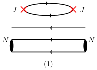
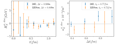
Figure S 1: Upper panel: two disconnected diagrams computed in this work. Lower panel (left): hadronic functions $H^{ii}(t)$ obtained from disconnected diagrams as a function of $t$ with $\Delta t$ fixed at 0.96 fm (24D) and 0.86 fm (32Dfine). Lower panel (right): the contributions to polarizabilities from disconnected diagrams, $\alpha_{E}^{ii,disc}$, as a function of $\Delta t$ with the temporal truncation set as $t_{0}=0.77$ fm (24D) and 0.72 fm (32Dfine).

V.3 Quark-field contractions for $N\pi$ scattering and $N+\gamma^{*}\to N\pi$ transition

The $N\pi$ operators for different isospin channels are listed below

$$O_{N\pi}^{I=\frac{1}{2},I_{3}=\frac{1}{2}} = \frac{1}{\sqrt{3}}(\sqrt{2}O_{n}O_{\pi^{+}}+O_{p}O_{\pi^{0}}),$$

$$O_{N\pi}^{I=\frac{1}{2},I_{3}=-\frac{1}{2}} = \frac{1}{\sqrt{3}}(-O_{n}O_{\pi^{0}}+\sqrt{2}O_{p}O_{\pi^{-}}),$$

$$O_{N\pi}^{I=\frac{3}{2},I_{3}=\frac{1}{2}} = \frac{1}{\sqrt{3}}(O_{n}O_{\pi^{+}}-\sqrt{2}O_{p}O_{\pi^{0}}),$$

$$O_{N\pi}^{I=\frac{3}{2},I_{3}=-\frac{1}{2}} = \frac{1}{\sqrt{3}}(-\sqrt{2}O_{n}O_{\pi^{0}}-O_{p}O_{\pi^{-}}).$$ (S 21)

The correlation functions for the $N\pi$ scattering

$$C_{N\pi}^{I}(t_{f},t_{i})=\langle O_{N\pi}^{I,I_{3}}(t_{f})O_{N\pi}^{I,I_{3},\dagger}(t_{i})\rangle$$ (S 22)

encompass contributions from 19 distinct diagrams with

$$C_{N\pi}^{I=\frac{1}{2}} = \frac{1}{2}\left\{2D_{1}-2D_{2}-3D_{3}-2D_{4}-2D_{5}+3D_{6}+3D_{7}\right.$$

$$+3D_{8}+2D_{9}-3D_{10}-3D_{11}+3D_{12}+D_{13}$$

$$\left.-D_{14}-D_{15}-D_{16}+D_{17}+D_{18}-D_{19}\right\},$$

$$C_{N\pi}^{I=\frac{3}{2}} = D_{1}-D_{2}-D_{4}-D_{5}+D_{9}-D_{13}+D_{14}+D_{15}$$ (S 23)

$$+D_{16}-D_{17}-D_{18}+D_{19}.$$

Here $D_{i}$ ($i=1,2\cdots,19$) designates the $i_{\mathrm{th}}$ type of contraction diagram, as illustrated in Fig. S 2.

Figure S 2: Contractions for $N\pi$ scattering.

The correlation functions relevant to the $N\gamma^{*}\to N\pi$ transition are given as

$$C_{NJN\pi}^{I,I^{\prime}}(t_{f},t,t_{i})=\langle O_{N\pi}^{I,I_{3}}(t_{f})J_{i}^{I^{\prime}}(t)O_{N}^{\dagger}(t_{i})\rangle$$ (S 24)

where $I^{\prime}$ signifies the isospin carried by the vector current, while $I$ and $I_{3}$ denote the isospin attributes of the $N\pi$ state. These correlation functions incorporate contributions from $20$ diagrams with

$$C_{pJN\pi}^{\frac{1}{2},0} = -i\frac{\sqrt{2}}{4}\left\{-E_{3}+E_{6}+E_{7}-E_{8}+E_{10}-E_{11}\right.$$

$$+E_{12}-E_{13}+E_{14}+E_{15}-E_{16}+E_{17}$$

$$\left.-E_{18}+E_{19}-2E_{20}\right\},$$

$$C_{pJN\pi}^{\frac{1}{2},1} = -i\frac{\sqrt{2}}{4}\left\{2E_{1}-2E_{2}-3E_{3}-2E_{4}-2E_{5}+3E_{6}\right.$$

$$+3E_{7}+3E_{8}+2E_{9}-3E_{10}-3E_{11}+3E_{12}$$

$$\left.+E_{13}-E_{14}-E_{15}-E_{16}+E_{17}+E_{18}-E_{19}\right\},$$

$$C_{pJN\pi}^{\frac{3}{2},1} = i\left\{E_{1}-E_{2}-E_{4}-E_{5}+E_{9}-E_{13}+E_{14}\right.$$ (S 25)

$$\left.+E_{15}+E_{16}-E_{17}-E_{18}+E_{19}\right\}.$$

Here $E_{i}$ ($i,=1,2,\cdots,20$) denotes the $i_{\mathrm{th}}$ type of contraction diagram, as depicted in Fig. S 3. When substituting the neutron for the proton in the initial state, the pertinent correlation functions are directly related to those in the proton case, as shown below

$$C_{nJN\pi}^{\frac{1}{2},0}=C_{pJN\pi}^{\frac{1}{2},0},\quad C_{nJN\pi}^{\frac{1}{2},1}=-C_{pJN\pi}^{\frac{1}{2},1},\quad C_{nJN\pi}^{\frac{3}{2},1}=C_{pJN\pi}^{\frac{3}{2},1}.$$ (S 26)

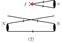
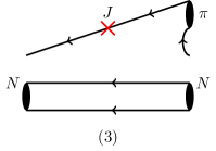
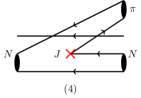
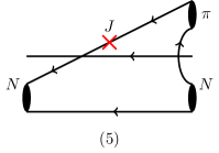
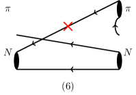
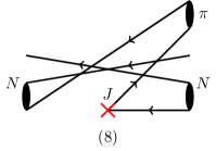
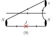
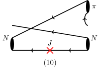
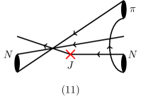
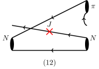
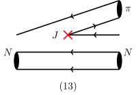
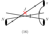
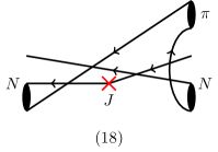
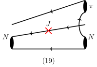
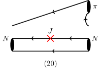
Figure S 3: Contractions for $N\gamma^{*}\to N\pi$ transition.