Online Permutation Tests: $e$-values and Likelihood Ratios for Testing Group Invariance

Abstract

We develop a flexible online version of the permutation test. This allows us to test exchangeability as the data is arriving, where we can choose to stop or continue without invalidating the size of the test. Our methods generalize beyond exchangeability to other forms of invariance under a compact group. Our approach relies on constructing an $e$-process that is the running product of multiple conditional $e$-values. To construct $e$-values, we first develop an essentially complete class of admissible $e$-values in which one can flexibly ‘plug in’ almost any desired test statistic. To make the $e$-values conditional, we explore the intersection between the concepts of conditional invariance and sequential invariance, and find that the appropriate conditional distribution can be captured by a compact subgroup. To find powerful $e$-values for given alternatives, we develop the theory of likelihood ratios for testing group invariance yielding new optimality results for group invariance tests. These statistics turn out to exist in three different flavors, depending on the space on which we specify our alternative. We apply these statistics to test against a Gaussian location shift, which yields connections to the $t$-test when testing sphericity, connections to the softmax function and its temperature when testing exchangeability, and yields an improved version of a known $e$-value for testing sign-symmetry. Moreover, we introduce an impatience parameter that allows users to obtain more power now in exchange for less power in the long run.

Keywords: $e$-values, sequential testing, online testing, group invariance test, permutation test.

1 Introduction

1.1 Motivating example

We introduce and motivate our methodology through an example: a case-control study. In an idealized traditional case-control study, treatments are randomly allocated across $n$ units at the start of the study. The null hypothesis $H_{0}^{\text{static}}$ that the treatment has no effect can be represented as

$$H_{0}^{\text{static}}:X_{[1:n]}\text{ is exchangeable},$$

where $X_{[1:n]}=X_{1},\dots,X_{n}$ denotes the observed outcomes. Exchangeability here means that $X_{[1:n]}$ is equal in distribution to $PX_{[1:n]}$, where $P$ denotes a permutation. We will use $\mathfrak{P}_{n}$ to denote the collection of permutations on $n$ elements

To test this null hypothesis at some level $\alpha$, we can select any desired real-valued test statistic $T$ and perform a permutation test. The $p$-value for this test is defined as

$$p(X_{[1:n]})=\mathbb{P}_{\overline{P}}\left(T(\overline{P}X_{[1:n]})\geq T(X_{[1:n]})\right)+\overline{u}\mathbb{P}_{\overline{P}}\left(T(\overline{P}X_{[1:n]})=T(X_{[1:n]})\right),$$

where $\overline{P}$ is uniformly distributed on $\mathfrak{P}_{n}$ and $\overline{u}$ is uniform on $[0,1]$. This $p$-value can be understood as the proportion of test statistics calculated from the rearranged (‘permuted’) data that exceed or match the original test statistic, and a small correction to handle discreteness. Moreover, it is guaranteed to be exact in finite samples:

$$\mathbb{P}\left[p(X_{[1:n]})\leq\alpha\right]=\alpha,\text{ for all }n.$$

Unfortunately, it is hard to determine a ‘good’ sample size $n$ prior to the study, as the magnitude of the treatment effect under the alternative is usually unknown. If the sample size $n$ is set too small, there is a high risk of not rejecting the null hypothesis, even if the treatment is effective On the other hand, setting $n$ too large may come with higher cost or ethical concerns.

As $n$ is hard to specify ahead of time, we would ideally choose it in an ‘online’ fashion, based on the data that has already arrived. However, we cannot simply use this ‘static’ permutation test with a dynamic number of observations, as the resulting test would not have valid ‘sequential size’. Indeed, we typically do not have

$$\mathbb{P}\left[\inf_{n\in\mathbb{T}}p(X_{[1:n]})\leq\alpha\right]\leq\alpha,$$ (1)

where $\mathbb{T}=\{t_{1},t_{2},\dots\}$ contains the points in time at which we would like to perform our test. This means that even if there is no treatment effect, our $p$-value will eventually drop below the threshold $\alpha$ with a probability that is typically much higher than $\alpha$.

The primary contribution of this paper is to introduce an online generalization of the permutation test that does have valid sequential size. The test we introduce is valid for multiple different types of sequential treatment allocations that lead to different null hypotheses. We will refer to two of the most important resulting hypotheses as sequential exchangeability and within-batch exchangeability.

Sequential exchangeability. Here, the treatments are randomly allocated at the beginning of the study, with outcomes $X=X_{1},X_{2},\dots$ observed sequentially. The null hypothesis that posits no treatment effect can then be formulated as

$$H_{0}^{\text{exch}}:X\text{ is sequentially exchangeable},$$

where sequential exchangeability means that $X_{[1:n]}$ is exchangeable for all $n$, and $[1$:$n]$ denotes the range of indices from $1$ to $n$, where $n\geq 1$.

Within-batch exchangeability. Here, the treatment allocation is not decided at the start. Instead, treatments are only allocated to the first batch of units at the start, after which their outcomes are observed. Based on these outcomes, treatments may be independently allocated to new batches, and the choice to allocate further treatments can be made after every batch. We then formulate our null hypothesis of no treatment effect as

$$H_{0}^{\text{batch}}:X\text{ is within-batch exchangeable}.$$

Here, we do not assume that the batches are independent under the null hypothesis, but we do assume that the random treatment allocation process is independent from the previous batches. For example, this means that the number of observations collected in the next batch can be based on the previously observed batches.

Another potential allocation scheme may result in across-batch exchangeability, where the batches themselves are exchangeable units. However, this is nested in sequential exchangeability, if one considers each $X_{1}$, $X_{2}$, …to represent a batch.

Observe that $H_{0}^{\text{exch}}\implies H_{0}^{\text{batch}}$, as a sequentially exchangeable $X$ is certainly also within-batch exchangeable. We demonstrate that both are special cases of a broader class of sequential invariance hypotheses, for which we will introduce our methodology.

1.2 Contributions

Our primary contribution is the construction of ‘online’ group invariance tests for testing sequential invariance under a sequence of compact groups. This includes online permutation tests for sequential exchangeability and within-batch exchangeability, as well as online $t$-tests for spherical invariance, and many other possibilities. In the construction of these tests, we rely on the recently popularized $e$-values (sometimes $e$-variables or $e$-statistics) and $e$-processes, which are detailed in Section 2.

Our primary technical contribution is the development of the theory of conditional invariance and its intersection with sequential invariance, which plays a key role in the development of our $e$-processes. In particular, we show that the conditional distribution of an invariant sequence of random variables given the past data, can be characterized by a ‘conditioning subgroup’. Moreover, we find that online testing of sequential group invariance with a martingale can be interpreted as testing sequential invariance under a sequence of such conditioning subgroups. If these subgroups are trivial, then no martingale-based test has more than trivial power. This generalizes an impossibility result that Ramdas et al. (2022b) derived for the special case of sequential exchangeability and binary data. For sequential exchangeability, this issue was also observed by Vovk (2021).

To construct our tests, we start by introducing ‘generic’ $e$-values for group invariance, that can use any (appropriately integrable) test statistic, that is allowed to be chosen based on the past data. We show that the class of these $e$-values constitutes an essentially complete class of admissible $e$-values, so that we are not missing out on any ‘good’ $e$-values. Our $e$-processes are then constructed by multiplying together a sequence of conditional $e$-values, which are constructed from conditioning subgroups.

To find powerful $e$-values for alternatives of interest, we develop the theory of likelihood ratio statistics for group invariance. To the best of our knowledge, such likelihood ratio statistics have not been explicitly derived before. Likelihood ratio processes are $e$-processes (Ramdas et al., 2023), and are known to have attractive power properties in a sequential testing setting (Koolen & Grünwald, 2022; Grünwald et al., 2023).

We find that these likelihood ratios come in three distinct flavors, that depend on the space on which the alternative is specified. The first flavor relies on specifying an alternative on the sample space, and is inspired by an old proof strategy of Lehmann & Stein (1949) for proving optimality of group invariance tests. For the second flavor, we instead specify an alternative on invariant subsets (orbits). As a side-contribution, we explain how we can use this second flavor to generalize the optimality result of Lehmann & Stein (1949) to certain composite alternatives. The third flavor relies on specifying an alternative on the group itself. For this flavor, we use an inversion kernel (see Ch. 7 in Kallenberg 2017), which was recently introduced in the context of group invariance testing by Chiu & Bloem-Reddy (2023). A toy example of these different types of likelihood ratios can be found in Appendix A.

We apply our likelihood ratio statistics to testing group invariance on $\mathbb{R}^{d}$, $d\geq 1$, against a simple alternative that is a location shift under normality. For the special case of spherical invariance, this is connected to an example from Lehmann & Stein (1949) regarding the optimality of the $t$-test, which we generalize to derive a larger class of alternatives against which the $t$-test is uniformly most powerful. We also consider sign-symmetry, which produces an $e$-value that can be viewed as an admissible version of an $e$-value derived by de la Peña (1999). Furthermore, we consider exchangeability where we find that the softmax function is nested as a special case of our likelihood ratio statistic. In addition, we provide some guidance for composite alternatives, on how we can mix over a composite alternative, or attempt to learn the alternative.

Finally, we introduce an impatience parameter into our $e$-values that allows a user to specify whether they want more power now or more power in the future. We show that this impatience parameter has a nice interpretation, in that it increases the variance of the $e$-value, but at the same time decreases its growth rate.

1.3 Related literature

At first glance, our work may seem intimately related to the work of Pérez-Ortiz et al. (2022). However, they consider invariance of collections of distributions (both the null and the alternative), whereas we consider invariance of distributions themselves. Specifically, a collection of distributions $\mathcal{P}$ is said to be invariant under a transformation $g$ if for any $\mathbb{P}\in\mathcal{P}$, its transformation $g\mathbb{P}$ by $g$ is also in $\mathcal{P}$. In contrast, invariance of a distribution $\mathbb{P}$ means that its transformation $g\mathbb{P}$ is equal to $\mathbb{P}$ itself. Intuitively, their work can be interpreted as testing in the presence of an invariant model, whereas we consider testing the invariance of the data generating process.

As our null hypothesis consists exclusively of invariant distributions it is technically also invariant, so that one may believe their results may still apply under appropriate assumptions on the alternative. However, this invariance is of a very strong type which excludes the transitivity that Pérez-Ortiz et al. (2022) require. In some sense, the strong type of invariance we consider is the complete opposite of transitivity.

A closely related work is that of Ramdas et al. (2022b), who consider testing for sequential exchangeability $H_{0}^{\text{exch}}$. However, they focus primarily on the case where $X=X_{1},X_{2},\dots$ is a binary or $d$-ary sequence. Their methods rely on taking an infimum over multiple non-negative supermartingales, which itself is no longer a supermartingale, but is still an $e$-process. It is not clear how their methods can be extended beyond $d$-ary data, nor to other forms of group invariance.

Another related work is that of Vovk (2021), who also study sequential exchangeability. They exploit the fact that the sequential ranks are independent from the past ranks under sequential exchangeability. They then convert these ranks into independent $e$-values, which they multiply together to construct an $e$-process. There are two key differences between their approach and ours. First, their approach forces one to use the ranks as a test statistic. Second, they only allow inspection of the previous $p$-values, whereas we allow full inspection of all the previous data. See Section 3.6 for more details on how their approach nests within our general framework. Moreover, their methods do not easily generalize to other forms of group invariance.

A link between the softmax function and $e$-values for exchangeability was also made in unpublished early manuscripts of Wang & Ramdas (2022) and Ignatiadis et al. (2023), which they call a ‘soft-rank’ $e$-value. In Remark 6, we explore the connection to our softmax $e$-value, and find that their soft-rank $e$-value can be interpreted as a ‘riskier’ variation of ours.

For more recent work in the context of sequential case-control (or ‘A/B’) testing see Johari et al. (2022) and Larsen et al. (2023), who do not consider exchangeability.

1.4 Notation and assumptions

We assume the random variables $X_{1},X_{2},\dots$ that we observe take on values in locally compact second-countable Hausdorff topological spaces $\mathcal{X}_{1},\mathcal{X}_{2},\dots$, which includes $\mathbb{R}^{n}$, $n\geq 1$. We equip $\mathcal{X}_{i}$ with its Borel $\sigma$-algebra $\mathcal{B}(\mathcal{X}_{i})$. We write $\mathcal{X}^{m}=\prod_{i=1}^{m}\mathcal{X}_{i}$ and $\mathcal{B}(\mathcal{X}^{m})=\prod_{i=1}^{m}\mathcal{B}(\mathcal{X}_{i})$ for the product space and its Borel $\sigma$-algebra, $m\in\mathbb{N}_{+}\cup\{\infty\}$.

To avoid ambiguity, we sometimes write expectations $\mathbb{E}$ with a superscript and/or subscript $\mathbb{E}_{X}^{\mathbb{P}}$ to make explicit the measure over which is being integrated ($\mathbb{P}$), and the random variables over which the integration takes place ($X$). We use similar subscripts for probabilities. Moreover, we use $\mathbb{E}_{\mathbb{P}}^{Q}\mathbb{P}$ to denote a $Q$-mixture over $\mathbb{P}$. For any collection of indices $\mathcal{I}\subset\mathbb{N}_{+}$, we use $X_{\mathcal{I}}$ to denote the corresponding subset of $X$, and we use $[s$:$t]$ to denote the set of indices from $s$ to $t$, and $[s$:$t)$ to denote the same set excluding $t$. Moreover, we use $X$ to denote the entire sequence: $X=X_{1},X_{2},\dots$.

2 Background: $e$-values and $e$-processes

”A new perspective on testing that has garnered much recent attention is the use of so-called $e$-values (or $e$-statistics, $e$-variables). For an overview of the rapidly developing literature on $e$-values, see, for example, Ramdas et al. (2023).

For an arbitrary collection of distributions $\mathcal{P}$, typically a null hypothesis, an $e$-value is defined as some non-negative real-valued test statistic $e$ with the property

$$\sup_{\mathbb{P}\in\mathcal{P}}\mathbb{E}^{\mathbb{P}}e\leq 1.$$ (2)

We call such an $e$-value ’valid’ for $\mathcal{P}$. If it satisfies $\sup_{\mathbb{P}\in\mathcal{P}}\mathbb{E}_{e}^{\mathbb{P}}e=1$, we refer to it as ’exact’

Based on an $e$-value, a finite sample valid test is easily constructed by rejecting if $e\geq 1/\alpha$. Indeed, Markov’s inequality tells us that

$$\sup_{\mathbb{P}\in\mathcal{P}}\mathbb{P}_{e}\left(e\geq 1/\alpha\right)\leq\alpha.$$

The corresponding valid $p$-value, the smallest value of $\alpha$ for which the test rejects, is then given by $1/e$.

Of particular importance for our purposes, $e$-values have a sequential counterpart known as $e$-processes. An $e$-process for a collection of distributions $\mathcal{P}$ is a non-negative process $(e_{t})_{t\geq 1}$ with

$$\sup_{\mathbb{P}\in\mathcal{P}}\sup_{\tau}\mathbb{E}_{e_{\tau}}^{\mathbb{P}}[e_{\tau}]\leq 1,$$ (3)

where $\tau$ ranges over all stopping times (Ramdas et al., 2022b). The test that compares an $e$-process to $1/\alpha$ satisfies the desired ‘anytime validity’ property:

$$\sup_{\mathbb{P}\in\mathcal{P}}\mathbb{P}_{e_{t}}\left(\sup_{t\geq 1}e_{t}\geq 1/\alpha\right)\leq\alpha.$$ (4)

The corresponding valid $p$-value is $\inf_{t}1/e_{t}$. To see that this property holds, one can show that (4) is equivalent to $\sup_{\mathbb{P}\in\mathcal{P}}\sup_{\tau}\mathbb{P}_{e_{\tau}}\left(e_{\tau}\geq 1/\alpha\right)\leq\alpha$, apply Markov’s inequality to bound $\mathbb{P}_{e_{\tau}}\left(e_{\tau}\geq 1/\alpha\right)$ and invoke (3) (see Ramdas et al. (2022a) for a detailed discussion).

One should not view an $e$-process merely as ‘an $e$-value evaluated at time $t$’, since such a process would generally not yield a valid $e$-process. The trick lies in constructing a valid $e$-value at time $t$, conditional on the past data. By the law of total expectation, the running product of such $e$-values then yields a valid $e$-process (Ramdas et al., 2023). Such $e$-processes are also known as non-negative (super)martingales. In fact, all $e$-processes are almost surely bounded by some non-negative supermartingale (Ramdas et al., 2022a).

An important property of $e$-processes is that any mixture or infimum of $e$-processes remains an $e$-process.

Remark 1.

Wang & Ramdas (2023) further generalize $e$-processes by observing that it is sufficient that $\sup_{\mathbb{P}\in\mathcal{P}}\sup_{\tau}\mathbb{E}_{e_{\tau}}^{\mathbb{P}}[e_{\tau}\wedge 1/\alpha]\leq 1$. This for example permits $e$-processes defined on the extended non-negative reals. Furthermore, Ramdas & Manole (2023) propose a strictly more powerful (yet still valid) randomized testing approach, which rejects if the $e$-value or $e$-process exceeds $U/\alpha$, with $U$ being a random variable distributed uniformly on the unit interval $[0,1]$.

3 (Sequential) (conditional) group invariance

3.1 Group invariance and testing

Let $\mathcal{G}$ be a compact (second countable Hausdorff) topological group, acting continuously on some sample space $\mathcal{Y}$, say $\mathcal{Y}=\mathcal{X}^{m}$ for some $m\in\mathbb{N}_{+}$. Examples of compact groups acting on $\mathbb{R}^{m}$ include permutations, rotations, and sign-flips. Such groups can be represented by collections of orthonormal matrices that are closed under matrix multiplication and inverses, and act on $\mathbb{R}^{m}$ through matrix multiplication.

The ’orbit’ of $y\in\mathcal{Y}$, denoted by $O_{y}=\{z\in\mathcal{Y}\ |\ z=Gy,\ \exists G\in\mathcal{G}\},$ is the set of all points that can be reached from $y$ by applying an element of the group. An orbit can be interpreted as all the points we can reach from $y$ by applying an element of the group to it. We assign a single point $[y]$ on each orbit as the ‘orbit representative’ of $O_{y}$. That is, $[y]=Gy$ for some $G\in\mathcal{G}$. We use $[\mathcal{Y}]$ to denote the collection of orbit representatives, and $\mathcal{Y}/\mathcal{G}$ for the collection of all orbits, and we call the function $[\cdot]:\mathcal{Y}\to[\mathcal{Y}]$ that maps $y$ to its orbit representative $[y]$ an orbit selector.

We say that a random variable is $\mathcal{G}$ invariant if its law remains unchanged after a transformation by any element of $\mathcal{G}$.

Definition 1.

A random variable $Y$ is $\mathcal{G}$ invariant if $Y\overset{d}{=}GY,\text{ for all }G\in\mathcal{G}$.

This is equivalent to $Y\overset{d}{=}\overline{G}Y$, where $\overline{G}$ is uniform (Haar) distributed on $\mathcal{G}$ independently from $Y$. Moreover, it is equivalent to $Y\overset{d}{=}\overline{G}[Y]$, provided that the orbit selector is measurable. This means that an invariant random variable can be decomposed or deconvolved into a uniform random variable on the group multiplied by (using the group action) a distribution over orbit representatives. Alternatively, we can say that the conditional distribution of $Y$ given that $Y$ is on the orbit $O$ is uniform on $O$.

To test the null hypothesis $H_{0}^{\mathcal{G}}$ that $Y$ is $\mathcal{G}$ invariant, we can generalize the static permutation test for exchangeability. Given any test statistic $T:\mathcal{Y}\to\mathbb{R}$, a $p$-value can be defined as

$$p(Y)=\mathbb{P}_{\overline{G}}\left(T(\overline{G}Y)\geq T(Y)\right)+\overline{u}\mathbb{P}_{\overline{G}}\left(T(\overline{G}Y)=T(Y)\right),$$

where $\overline{G}$ is uniformly (Haar) distributed on $\mathcal{G}$, which is well-defined as $\mathcal{G}$ is compact, and $\overline{u}$ is uniform on $[0,1]$. Comparing this $p$-value to a significance level $\alpha\in[0,1]$ yields a so-called group invariance test. This test is equivalent to rejecting $H_{0}^{\mathcal{G}}$ if

$$T(Y)>q_{\alpha}^{\overline{G}}[T(\overline{G}Y)],$$ (5)

and with some appropriate probability in case of equality, where $q_{\alpha}^{\overline{G}}[T(\overline{G}Y)]$ denotes the $\alpha$ upper-quantile of the distribution of $T(\overline{G}Y)$ where $Y$ is considered fixed.

Rather than leaving the choice of test statistic flexible, another approach is to fix the choice of test statistic $T:\mathcal{Y}\to\mathbb{R}$. The group action of $\mathcal{G}$ on $\mathcal{Y}$ induces a group action on the map $T$. This group action can be defined as $GT(Y)=T(G^{-1}Y)$. Note that this group action should not be interpreted as an action on the codomain on $T$, but rather on some implicitly defined space of test statistics. To the best of our knowledge, it was first observed by Kashlak (2022) that we can incorporate our test statistic into the null hypothesis:

$$[\overline{G}T](Y)\overset{d}{=}T(Y).$$

Hence, given the choice of test statistic, this is the invariance that we are implicitly testing.

3.2 Sequential group invariance

A sequential analogue of group invariance can be introduced as follows. Consider a ‘nested’ sequence of compact groups $(\mathcal{G}_{n})_{n\geq 1}$, where $\mathcal{G}_{n}\subseteq\mathcal{G}_{n+1}$, and $\mathcal{G}_{n}$ acts continuously on $\mathcal{X}^{n}$ for every $n$.

We assume that the group actions in the sequence are compatible. In particular, we assume that the orbits are nested: for any $y_{n+1}\in\mathcal{X}^{n+1}=\mathcal{X}_{1}\times\cdots\times\mathcal{X}_{n+1}$, we have $\textnormal{proj}_{\mathcal{X}^{n}}(O_{y_{n+1}})\supseteq O_{\textnormal{proj}_{\mathcal{X}^{n}}(y_{n+1})}$, where $\textnormal{proj}_{\mathcal{X}^{n}}$ denotes the usual projection map from $\mathcal{X}^{n+1}$ to $\mathcal{X}^{n}$ under the Cartesian product. An interpretation is that more information about the eventual orbit is revealed with each observation. Taking $m>n$, this ensures that $\mathcal{G}_{m}$ invariance is a stronger property than $\mathcal{G}_{n}$ invariance, so that rejecting $\mathcal{G}_{n}$ invariance will allow us to reject $\mathcal{G}_{m}$ invariance, and size control for $\mathcal{G}_{n}$ invariance implies size control for $\mathcal{G}_{m}$ invariance.

Having defined this sequence of groups, we can define a notion of sequential invariance.

Definition 2 (Sequential invariance).

$X=X_{1},X_{2},\dots$ is $(\mathcal{G}_{n})_{n\geq 1}$ invariant if $X_{[1:n]}$ is $\mathcal{G}_{n}$ invariant for all $n$.

Example 1 (Sequential exchangeability).

If we choose $\mathcal{G}_{n}$ to equal the group $\mathfrak{P}_{n}$ of permutations on $n$ elements for every $n$, then we recover sequential exchangeability as in $H_{0}^{\text{exch}}$. For example, if we sequentially observe the binary string $101$, then the orbits are $O_{1}=\{1\}$, $O_{10}=\{10,01\}$ and $O_{101}=\{101,110,011\}$. Notice that the nesting property is satisfied: $\textnormal{proj}_{\mathcal{X}^{1}}(O_{10})=\{1,0\}\supseteq O_{1}=O_{\textnormal{proj}_{\mathcal{X}^{1}}(10)}$, and $\textnormal{proj}_{\mathcal{X}^{2}}(O_{101})=\{10,11,01\}\supseteq O_{10}=O_{\textnormal{proj}_{\mathcal{X}^{2}}(101)}$.

Example 2 (Within-batch exchangeability).

Suppose that we sequentially observed batches of data $X_{1},X_{2},\dots$, that are each within-batch exchangeable. We can choose $\mathcal{G}_{n}=\mathfrak{P}^{1}\times\mathfrak{P}^{2}\times\cdots\times\mathfrak{P}^{n}$, where $\mathfrak{P}^{i}$ is the group of permutations acting on the batch $X_{i}$. Within-batch exchangeability can be viewed as invariance of $X=X_{1},X_{2},\dots$ under $(\mathcal{G}_{n})_{n\geq 1}$. Here, we actually have $\textnormal{proj}_{\mathcal{X}^{n}}(O_{X_{[1:n+1]}})=O_{\textnormal{proj}_{\mathcal{X}^{n}}(X_{[1:n+1]})}$, as the orbit factorizes: $O_{X_{[1:n+1]}}=O_{X_{[1:n]}}\times O_{X_{n+1}}$.

3.3 Conditional invariance

To construct our $e$-processes, we require a notion of conditional invariance. Indeed, we want to construct an $e$-value conditional on the previously observed data $X_{[1:n)}$, as these $e$-values form the building blocks for $e$-processes.

Our aim is not merely to define an invariant conditional distribution. Rather, our objective is to begin with a $\mathcal{G}$ invariant random variable and derive a conditional distribution. Specifically, we are interested in finding the conditional distribution of a $\mathcal{G}$ invariant random variable $Y$ given both its orbit $O$ and $h(Y)$, where $h$ is some function of $Y$. In particular, we consider $h$ to be a continuous function mapping $\mathcal{Y}$ into a (Hausdorff) topological space. Then, let us define the subset of $\mathcal{G}$ consisting of elements that leave $h(y)$ unchanged:

$$\mathcal{S}^{h}(y)=\{G\in\mathcal{G}:h(Gy)=h(y)\}.$$

This set forms a compact group, henceforth referred to as the conditioning stabilizer under $h$. See Appendix C.1 for a proof.

Lemma 1.

$\mathcal{S}^{h}(y)$ is a compact subgroup of $\mathcal{G}$.

Theorem 1 establishes a connection between the conditional distribution of $Y$, given $h(Y)$, and the conditioning stabilizer. In particular, given $h(Y)$ and the orbit of $Y$, the conditional distribution of $Y$ can be characterized using $\mathcal{S}_{n}$. A proof is given in Appendix C.2.

Theorem 1.

Let $\overline{S}^{h}$ be uniform on $\mathcal{S}^{h}(Y)$. The conditional distribution of $Y$ given $h(Y)$ and some orbit $O\in\mathcal{Y}/\mathcal{G}$, is equal to the distribution of $\overline{S}^{h}z$, where $z\in O$ and $h(Gz)=h(z)$ for some $G\in\mathcal{G}$.

We can also use $Y$ itself to characterize this conditional distribution as,‘the distribution of $\overline{S}^{h}Y$, where $Y$ is considered fixed’. This implies that upon observing $Y$, we can simulate from this conditional distribution by sampling from $\overline{S}^{h}$ and applying the sampled transformations to the observed value of $Y$.

A consequence of Theorem 1 is that $Y$ is $\mathcal{S}^{h}(Y)$ invariant conditional on $h(Y)$. The same is also true for any compact subgroup of $\mathcal{S}^{h}(Y)$, but not for any (proper) supergroup of $\mathcal{S}^{h}(Y)$. Hence, the theorem does not merely tell us that $Y$ is $\mathcal{S}^{h}(Y)$ invariant conditional on $h(Y)$, but also that this invariance is ‘maximal’ in some sense.

3.4 Conditional group invariance given past data

Using the concept of conditional group invariance, we can describe the distribution of $X_{[1:n]}$ given $X_{[1:n)}$ for each orbit $O\in\mathcal{X}^{n}/\mathcal{G}_{n}$. For this purpose, consider the conditioning stabilizer

$$\mathcal{S}_{n}=\{G\in\mathcal{G}_{n}:\textnormal{proj}_{\mathcal{X}^{n-1}}(GX_{[1:n]})=\textnormal{proj}_{\mathcal{X}^{n-1}}(X_{[1:n]})\},$$ (6)

for $n\geq 2$ and $\mathcal{S}_{1}=\mathcal{G}_{1}$. Here, instead of using the notation $\mathcal{S}_{n}^{\textnormal{proj}_{\mathcal{X}^{n-1}}}$, we opt for $\mathcal{S}_{n}$ given the stabilizer’s significance in the sequential context.

Observe that $\textnormal{proj}_{\mathcal{X}^{n-1}}$ is continuous with respect to the product topology of $\mathcal{X}^{n}$. Hence, we can apply Lemma 1 to conclude that $\mathcal{S}_{n}$ is a compact subgroup of $\mathcal{G}_{n}$. Moreover, by Theorem 1, we can obtain a characterization of the desired conditional distribution, as specified in Corollary 1.

Corollary 1.

Suppose that $X_{[1:n]}$ is $\mathcal{G}_{n}$ invariant. Let $\overline{S}_{n}$ be uniform on $\mathcal{S}_{n}$. Then, conditional on any orbit $O$ under $\mathcal{G}_{n}$ acting on $\mathcal{X}^{n}$, the conditional distribution of $X_{[1:n]}$ given $X_{[1:n)}$, is equal to the distribution of $\overline{S}_{n}y$, where $y\in O$ and the first $(n-1)$ elements of $y$ coincide with $X_{[1:n)}$.

Example 3 (Sequential exchangeability).

Continuing from Example 1, suppose that we have $n$ observations $X=X_{1},X_{2},\dots,X_{n}$ that are exchangeable. Then, assuming the realizations are distinct, the conditional stabilizer given $X_{[1:n)}$ only contains the identity: $\mathcal{S}_{n}=\{I_{n}\}$, for all $n$. To illustrate this, suppose that we fix $X_{[1:n)}$. In this case, the $n$th element $X_{n}$ cannot be swapped with any other element of $X_{[1:n]}$ without altering $X_{[1:n)}$. Consequently, the sole group action that fixes $X_{[1:n)}$ is the identity action. As a consequence, the conditional distribution of interest is degenerate, and simply a Dirac measure at the point $X_{[1:n]}$. Allowing duplicate elements, $\mathcal{S}_{n}$ can only interchange duplicates, resulting in an orbit identical to that of the group containing only the identity, leading to the same degenerate conditional distribution.

This will have dramatic consequences for the power of tests for sequential exchangeability, which we discuss in the next sections.

Example 4 (Within-batch exchangeability).

Building on Example 2, consider observing $n$ data batches, represented as $X_{1},X_{2},\dots,X_{n}$, each of which is within-batch exchangeable. Then, assuming the realizations in each batch are distinct, $\mathcal{S}_{n}=\{I^{1}\}\times\{I^{2}\}\times\cdots\times\{I^{n-1}\}\times\mathfrak{P}^{n}$, where $I^{i}$ denotes the identity permutation acting on $\mathcal{X}_{i}$, $i\leq n$. Therefore, the conditional distribution of interest behaves as if $X_{[1:n)}$ is fixed and we permute only within the final batch. This means that, on the orbit of $X_{[1:n]}$, the conditional distribution of the final batch $X_{n}$ is simply equal to its unconditional distribution.

3.5 Sequential conditional invariance and degeneracy

With a notion of conditional invariance, we can now define sequential conditional invariance.

Definition 3.

$X$ is conditionally $(\mathcal{G}_{n})_{n\geq 1}$ invariant if it is $(\mathcal{S}_{n})_{n\geq 1}$ invariant. Equivalently, if $X_{[1:n]}$ is $\mathcal{S}_{n}$ invariant for every $n$.

Any martingale-based $e$-processes rely on the conditional distribution given the past data. Hence, any such $e$-process can be interpreted as actually testing $(\mathcal{S}_{n})_{n\geq 1}$ invariance instead of $(\mathcal{G}_{n})_{n\geq 1}$ invariance. As a consequence, if testing $(\mathcal{S}_{n})_{n\geq 1}$ invariance is a hard or impossible problem, the same holds for testing $(\mathcal{G}_{n})_{n\geq 1}$ invariance. Indeed, it may happen that even though $(\mathcal{G}_{n})_{n\geq 1}$ has a rich group structure, $(\mathcal{S}_{n})_{n\geq 1}$ is simply the identity element for each $n$. As a consequence, the conditional distribution is degenerate for each $n$. This directly implies that the only valid (super)martingales that exist must be (almost surely) constants and therefore yield powerless tests.

A situation where this happens is for testing sequential exchangeability (see Example 5). In this setting, this issue was already observed by Vovk (2021) and Ramdas et al. (2022b). The only solution out of this problem, without moving away from a martingale-based $e$-process, is to weaken the conditioning. Or as Vovk (2021) puts it: ‘impoverish’ the filtration. We discuss such approaches in Section 3.6.

Remark 2.

A way to circumvent this problem altogether, is to use an $e$-process that is not a (super)martingale, which is the approach taken by Ramdas et al. (2022b) for sequentially exchangeable binary or $d$-ary data. In particular, they take an infimum over different (super)martingales. Unfortunately, it is not clear how to generalize this approach beyond binary or $d$-ary data.

Example 5 (Sequential exchangeability).

For testing sequential exchangeability, we have the degenerate situation $(\mathcal{S}_{n})_{n\geq 1}=(\{I_{n}\})_{n\geq 1}$, again assuming that $X_{[1:n]}$ does not contain duplicate elements. As $X$ is $(\{I_{n}\})_{n\geq 1}$ invariant regardless of the distribution of $X$, any testing method that controls size under $(\{I_{n}\})_{n\geq 1}$ necessarily controls size over all distributions, and so has trivial power. As supermartingales rely on the conditional distributions, they effectively test $(\mathcal{S}_{n})_{n\geq 1}$ invariance, and are therefore powerless.

Example 6 (Within-batch exchangeability).

For within-batch exchangeability, the conditional stabilizers $\mathcal{S}_{n}=\{I_{1}\}\times\cdots\times\{I_{n-1}\}\times\mathfrak{P}^{n}$ are not degenerate, again assuming that every $X_{i}$ does not contain duplicate elements, $i<n$.

As sequential exchangeability implies within-batch exchangeability, rejecting within-batch exchangeability also rejects sequential exchangeability. As a result, we can construct a martingale with power for sequential exchangeability by merging together several observations into batches. This comes at the opportunity cost of optionally stopping in between those observations.

3.6 Other types of conditioning: choosing $h$

In the previous section, we observed that if we condition on all the past data then the conditional distribution may become degenerate. The only way out of this issue is to weaken the conditioning. In our framework, this is equivalent to choosing a map $h$ different from $\textnormal{proj}_{\mathcal{X}^{n-1}}$. As long as this map is continuous, Theorem 1 guarantees that the resulting conditional distribution of $X_{[1:n]}$ given $h(X_{[1:n]})$ is still still described by a compact conditioning stabilizer $\mathcal{S}^{h}(X_{[1:n]})$. A downside of this approach is that we may no longer inspect all the past data, but only some function of it: $h(X_{[1:n]})$.

One straightforward approach is to not test at every time step $n$, but to wait for a batch of data to accumulate. This is achieved by choosing $h_{n}=\textnormal{proj}_{\mathcal{X}^{n-b}}$ at every $b$th observation, and $h_{n}=X_{[1:n]}$ otherwise. For testing sequential exchangeability this coincides exactly with within-batch exchangeability. This means that we lose the option to inspect data inside a batch, until the entire batch of data has arrived.

Moreover, we can take Kashlak (2022) type approach described in Section 3.1 by fixing our test statistic, and reducing the testing problem to $GT(Y)\overset{d}{=}T(Y)$ for all $G\in\mathcal{G}$. We can then define an induced conditioning stabilizer subgroup that depends on the test statistic $T$:

$$\widetilde{\mathcal{S}}_{n}^{h}(Y)=\{G\in\mathcal{G}:h(GT(Y))=h(T(Y))\}.$$

For example, we can choose $h$ so that all but the final value of the test statistic are fixed: $h(X_{[1:n]})=(T_{1}(X_{1}),\dots,T_{n}(X_{n-1}))$. Such an approach is taken by Vovk (2021) in the context of sequential exchangeability. As a test statistic, he chooses the rank of the current observations among all the past observations. He (implicitly) shows that for sequential exchangeability, this can yield a fully enriched induced conditioning stabilizer subgroup: $\widetilde{\mathcal{S}}_{n}^{h}(X_{[1:n]})=\mathcal{G}_{n}$, even though the standard conditioning stabilizer $\mathcal{S}_{n}$ is degenerate. A consequence of this approach is that we may no longer inspect all the past data, but only the past values of the test statistic, which may be perfectly acceptable in some applications. A downside of this approach is that it may be difficult to find the induced conditioning stabilizer subgroup $\widetilde{\mathcal{S}}_{n}^{h}(Y)$. In practice, this means that we have less flexibility in our choice of test statistic, since choosing another test statistic means that we have to derive another conditioning stabilizer.

4 Generic $e$-values and $e$-processes for invariance

In this section, we show how to construct a ‘generic’ exact $e$-value for invariance based on any arbitrary (appropriately integrable) test statistic. Moreover, we also show the converse: that any exact $e$-value can be written in such a form for some test statistic. As a consequence, the class of such $e$-values forms an essentially complete class of admissible $e$-values; any $e$-value outside of this class is dominated by some $e$-value inside the class. This means that we do not miss out on any ‘good’ $e$-values by restricting our attention to this class.

We then continue by showing how these generic $e$-values can be used as building blocks to construct generic $e$-processes for sequential invariance, by leveraging the notion of conditional invariance that we define in Section 3.

4.1 Generic $e$-values

Let $T^{+}:\mathcal{Y}\to\mathbb{R}_{+}$ be some arbitrary test statistic that is appropriately integrable on every orbit $O\in\mathcal{Y}/\mathcal{G}$. Namely $0<\mathbb{E}_{\overline{G}}T^{+}(\overline{G}Y)<\infty$. Based on this test statistic, we consider the $e$-value

$$e_{T^{+}}(Y)=\frac{T^{+}(Y)}{\mathbb{E}_{\overline{G}}T^{+}(\overline{G}Y)},$$ (7)

where $\overline{G}$ is uniformly distributed on the group $\mathcal{G}$. The interpretation is that $e_{T^{+}}(Y)$ is large if $T^{+}(Y)$ is large compared to its average value on the orbit of $Y$. Moreover, as we shall show in Section 5, if $T^{+}\geq 0$ and $T^{+}$ is non-zero integrable on $\mathcal{Y}$, then $e_{T^{+}}$ can be interpreted as a likelihood ratio for $\mathcal{G}$ invariance against a density proportional to $T^{+}$.

Alternatively, and without loss of generality, we can parametrize this class of $e$-values with a real-valued test statistic $T=\log T^{+}$, as

$$\frac{\exp\{T(Y)\}}{\mathbb{E}_{\overline{G}}\exp\{T(\overline{G}Y)\}},$$ (8)

assuming that $\exp\{T(\overline{G}Y)\}$ is appropriately integrable. We further discuss how these $e$-values can be tuned with a time-preference parameter in Section 7.

Theorem 2 not only shows that these $e$-values are exact, but also the converse: any exact $e$-value can be written as in (7). Moreover, as any non-exact but valid $e$-value can be trivially improved by adding a sufficiently small deterministic constant to it, this constitutes an essentially complete class of admissible $e$-values for the null hypothesis $H_{0}^{\mathcal{G}}$ that $Y$ is $\mathcal{G}$ invariant.

The result is not obvious, as $H_{0}^{\mathcal{G}}$ is a large composite hypothesis, and the denominator in (7) only takes the expectation over the group. Its proof can be found in Appendix C.3.

Theorem 2.

The class of statistics of the type $e_{T^{+}}$ equals the class of all exact $e$-values for $H_{0}^{\mathcal{G}}$. Moreover, this constitutes an essentially complete class of admissible $e$-values for $H_{0}^{\mathcal{G}}$.

By Theorem 2, we can turn any appropriately integrable test statistic $T$ into an exact $e$-value for the null hypothesis $H_{0}^{\mathcal{G}}$ of $\mathcal{G}$ invariance, including non-exact $e$-values. This means that we almost have the same freedom in choosing our test statistic as in the classical group invariance test. Moreover, it shows that by only considering $e$-values this type, we are not ‘missing’ any $e$-values that may be better.

4.2 Generic $e$-processes

We can use the generic $e$-values to construct generic $e$-processes for sequential invariance. Recall that $\mathcal{S}_{n}$ denotes the conditioning stabilizer subgroup from Sections 3.4 and 3.5, that leaves $X_{[1:n)}$ unchanged when applied to $X_{[1:n]}$.

Let $\overline{S}_{n}$ be uniformly distributed on $\mathcal{S}_{n}$. Then, we define our generic $e$-process $(e_{n})_{n\geq 1}$ as

$$e_{n}(X_{[1:n]})=\prod_{i=1}^{n}\frac{T_{i}(X_{[1:i]})}{\mathbb{E}_{\overline{S}_{i}}T_{i}(\overline{S}_{i}X_{[1:i]})}=\frac{\prod_{i=1}^{n}T_{i}(X_{[1:i]})}{\mathbb{E}_{\overline{S}_{1},\dots,\overline{S}_{n}}\prod_{i=1}^{n}T_{i}(\overline{S}_{i}X_{[1:i]})}$$ (9)

for test statistics $T_{i}:\mathcal{X}^{i}\to\mathbb{R}$, that can depend on the previously observed data. This $e$-process is indeed valid, by the following result. Its proof can be found in Appendix C.4, and relies on showing that the factors of the product are $e$-values conditional on the past data, and then applying the law of iterated expectations.

Theorem 3.

$(e_{n})_{n\geq 1}$ is an exact $e$-process for $(\mathcal{G}_{n})_{n\geq 1}$ invariance.

As a consequence of Theorem 3, we can construct an online group invariance test by rejecting as soon as this $e$-process exceeds $1/\alpha$.

Example 7 (Within-batch exchangeability $e$-process).

Let us continue our running example, where $X$ is observed sequentially in batches $X_{1}$, $X_{2}$, $\dots$ that are each internally exchangeable. Let $\overline{P}_{i}$ be uniformly distributed on the permutations on the $i$th batch $X_{i}$. Let $T_{i}$ be a test statistic that is allowed to be based on or estimated from the previous batches. Then, our generic $e$-process $(e_{n})_{n\geq 1}$ is defined as a running product of generic batch-wise $e$-values:

$$e_{n}(X_{[1:n]})=\prod_{i=1}^{n}\frac{T_{i}(X_{i})}{\mathbb{E}_{\overline{P}_{i}}T_{i}(\overline{P}_{i}X_{i})},$$ (10)

where $n$ is the number of observed batches. As sequential exchangeability implies within-batch exchangeability, this $e$-process is also valid for sequential exchangeability.

For the within-batch exchangeability setting, define $\mathcal{G}_{n}^{\dagger}=\mathcal{S}_{n}\mathcal{S}_{n-1}\cdots\mathcal{S}_{1}=\mathfrak{P}^{1}\times\cdots\times\mathfrak{P}^{n}$. Define $\mathfrak{T}_{n}:\mathcal{X}^{n}\to\mathbb{R}$ as $\mathfrak{T}_{n}(y_{[1:n]})=\prod_{i=1}^{n}T_{i}(y_{i})$, $y_{[1:n]}\in\mathcal{X}^{n}$. Then, this $e$-process can be more concisely written as

$$e_{n}(X_{[1:n]})=\frac{\prod_{i=1}^{n}T_{i}(X_{i})}{\mathbb{E}_{\overline{P}_{1},\dots\overline{P}_{n}}\prod_{i=1}^{n}T_{i}(\overline{P}_{i}X_{i})}=\frac{\mathfrak{T}_{n}(X_{[1:n]})}{\mathbb{E}_{\overline{G}_{n}^{\dagger}}\mathfrak{T}_{n}(\overline{G}_{n}^{\dagger}X_{[1:n]})},$$ (11)

where $\overline{G}_{n}^{\dagger}$ is uniformly distributed on $\mathcal{G}_{n}^{\dagger}$.

Remark 3.

It is well-known that any mixture or infimum of $e$-processes remains an $e$-process. Interestingly, by the flexible construction of these $e$-processes, we can also use a mixture or infimum of test statistics as a test statistic.

Remark 4.

If $\mathcal{G}_{n}^{\dagger}=\mathcal{S}_{n}\mathcal{S}_{n-1}\cdots\mathcal{S}_{1}$ is a compact group, which it is in a batch-wise group invariance setting, then we can concisely write

$$e_{n}(X_{[1:n]})=\frac{\mathfrak{T}_{n}(X_{[1:n]})}{\mathbb{E}_{\overline{G}_{n}^{\dagger}}\mathfrak{T}_{n}(\overline{G}_{n}^{\dagger}X_{[1:n]})},$$ (12)

where $\overline{G}_{n}^{\dagger}$ is uniform on $\mathcal{G}_{n}^{\dagger}$, and $\mathfrak{T}_{n}:\mathcal{X}^{n}\to\mathbb{R}$ is appropriately integrable and can depend on the previous data. A sufficient condition for $\mathcal{G}_{n}^{\dagger}$ to be a compact group is that $\mathcal{S}_{i}$ is a normal subgroup of $\mathcal{G}_{n}$ for every $i$.

4.3 Obtaining the normalization constant

The main computational challenge when using $(e_{n})_{n\geq 1}$ is the computing the normalization constant $\mathbb{E}_{\overline{G}}T_{+}(\overline{G}Y)$. While the conditioning subgroups $\mathcal{S}_{n}$ are typically much smaller than $\mathcal{G}_{n}$, they can still be enormous. As a consequence, the normalization constant $\mathbb{E}_{\overline{S}_{n}}T(\overline{S}_{n}y)$ in the denominator of (9) may need to be estimated. To do this, we can borrow ideas from the literature on group invariance testing.

The simplest idea is to use a Monte Carlo approach by replacing $\overline{S}_{n}$ with a random variable $\overline{S}_{n}^{M}$ that is uniformly distributed on a set of i.i.d. draws $\{\overline{S}_{n}^{(1)},\overline{S}_{n}^{(2)},\dots,\overline{S}_{n}^{(M)}\}$ of $\overline{S}_{n}$. Alternatively, we can replace $\overline{S}_{n}$ with $\overline{H}_{n}$ that is uniformly distributed on a compact subgroup of $\mathcal{S}_{n}$ (Chung & Fraser, 1958). As invariance under $\mathcal{S}_{n}$ implies invariance under every subgroup, this is still guaranteed to deliver a valid test, which is not clear for the Monte Carlo approach. Such a subgroup may also be easier to find or work with than $\mathcal{S}_{n}$ itself, making this approach more convenient. Moreover, Koning & Hemerik (2023) note that we can actually strategically select the subgroup based on the test statistic and alternative, and select a subgroup that yields high power. Koning (2023) notes that this can even yield tests that are more powerful than if we use the entire group $\mathcal{G}$.

Note that in the standard group invariance test, the goal is to estimate the $\alpha$-upper quantile of a reference distribution, as in (5). The normalization constant is the mean of this same distribution, which we expect to be much easier to estimate in practice. Based on simulation results, it seems that roughly 100 draws is usually sufficient. Moreover, in Appendix B we discuss that we can sometimes very efficiently approximate the normalization constant analytically.

5 Likelihood ratios for group invariance

The construction in the previous section gives us a lot of freedom when choosing an $e$-value. Unfortunately, this freedom also comes with the responsibility to select the $e$-value appropriately. For testing a simple null hypothesis against a simple alternative, $e$-processes built from likelihood ratio statistics have been shown to have attractive power properties (Koolen & Grünwald, 2022; Grünwald et al., 2023). Moreover, Ramdas et al. (2022a) show that any admissible procedure for online inference must rely on likelihood ratios.

For this reason, we derive likelihood ratio statistics for group invariance, which are well-specified and exact $e$-values even though the null hypothesis is highly composite. It turns out that these likelihood ratio statistics come in three flavors, where the flavor depends on the space on which we specify our alternative. For the first flavor, we specify an alternative on the entire sample space $\mathcal{Y}$. This type is inspired by a proof strategy of Lehmann & Stein (1949), who did not explicitly construct the likelihood ratio statistic but only derived a test that is equivalent to the likelihood ratio test (see Remark 5). For the second flavor, we do not specify an alternative on $\mathcal{Y}$, but we specify an alternative on every orbit. Although the orbits partition the sample space, this strictly generalizes the first flavor, as we need not specify the mixing distribution over the orbits. For the third and final flavor, we specify an alternative on the group $\mathcal{G}$. While we do not directly observe an element on our group, we use a so-called inversion kernel (Kallenberg, 2017) to obtain such an element.

The ideas in this section are applied in Section 6 to testing a location shift under Gaussianity against various types of invariances. Moreover, we include a toy example in Appendix A to illustrate the concepts.

5.1 Alternative on the sample space $\mathcal{Y}$

Suppose that $\mathbb{P}_{\mathcal{Y}}$ is our alternative on $\mathcal{Y}$, dominated by some measure $\lambda$, so that we can define the density $d\mathbb{P}_{\mathcal{Y}}/d\lambda$. A likelihood ratio statistic for testing this alternative against $\mathcal{G}$ invariance is presented in Theorem A proof is presented in Appendix C.5.

Theorem 4.

Let $\overline{G}$ be uniform $\mathcal{G}$ and assume that $0<\mathbb{E}_{\overline{G}}d\mathbb{P}_{\mathcal{Y}}/d\lambda(\overline{G}y)<\infty$ for all $y\in\mathcal{Y}$. Then, the statistic

$$\frac{d\mathbb{P}_{\mathcal{Y}}/d\lambda(y)}{\mathbb{E}_{\overline{G}}d\mathbb{P}_{\mathcal{Y}}/d\lambda(\overline{G}y)}$$ (13)

is a likelihood ratio statistic for testing $\mathcal{G}$ invariance against $\mathbb{P}_{\mathcal{Y}}$.

Note that this coincides with our $e$-value with the statistic $T_{+}=d\mathbb{P}_{\mathcal{Y}}/d\lambda$. The result also holds if $T_{+}$ is merely proportional to a density, as the proportionality constant drops out. Hence, for a statistic $T_{+}$ that is proportional to a density on $\mathcal{Y}$, we can interpret the resulting $e$-value as a likelihood ratio statistic against this density.

Remark 5.

The proof of Theorem 4 mimics the proof strategy of Theorem 2 and 2^′ in Lehmann & Stein (1949). They do not explicitly derive this likelihood ratio statistic. Instead, they show that the group invariance test based on the statistic $d\mathbb{P}_{\mathcal{Y}}/d\lambda$,

$$d\mathbb{P}_{\mathcal{Y}}/d\lambda(y)>q_{\alpha}^{\overline{G}}\left(d\mathbb{P}_{\mathcal{Y}}/d\lambda(\overline{G}y)\right),$$ (14)

is equivalent to a likelihood ratio test and hence uniformly most powerful for testing $\mathcal{G}$ invariance against $\mathbb{P}_{\mathcal{Y}}$ by the Neyman-Pearson lemma. We suspect that they did not explicitly compute the likelihood ratio statistic itself as the test in (14) is a much more efficient representation of the likelihood ratio test. Indeed, it is equivalent to the test

$$\frac{d\mathbb{P}_{\mathcal{Y}}/d\lambda(y)}{\mathbb{E}_{\overline{G}}d\mathbb{P}_{\mathcal{Y}}/d\lambda(\overline{G}y)}>q_{\alpha}^{\overline{G}}\left(\frac{d\mathbb{P}_{\mathcal{Y}}/d\lambda(\overline{G}y)}{\mathbb{E}_{\overline{G}_{2}}d\mathbb{P}_{\mathcal{Y}}/d\lambda(\overline{G}_{2}y)}\right),$$

but does not require the computation of the normalization constants.

5.2 Alternative on the orbits

In the previous section we defined an alternative on the entire sample space $\mathcal{Y}$. However, a careful inspection of the proof shows that we only compare the likelihood of $y$ to the likelihood of other values on its orbit. This implies that the likelihood ratio statistic only uses the conditional distributions on the orbits, and ‘discards’ the mixing distribution over the orbits.

As a consequence, we can also define a likelihood ratio statistic by specifying an alternative on every orbit. Specifically, let us choose a distribution $\mathbb{P}_{z}$ on each orbit $O_{z}$ and select $\lambda_{[z]}$ as the unique $\mathcal{G}$ invariant (uniform) distribution on $O_{z}$, $z\in[\mathcal{Y}]$. Then, we can construct a likelihood ratio statistic for each orbit:

$$\frac{d\mathbb{P}_{z}/d\lambda_{z}(y)}{\mathbb{E}_{\overline{G}}d\mathbb{P}_{z}/d\lambda_{z}(\overline{G}y)}=d\mathbb{P}_{z}/d\lambda_{z}(y),$$

where $z\in[\mathcal{Y}]$, $y\in O_{z}$, and the equality follows from the fact that the denominator is equal to 1 on each orbit, as it is a density on the orbit. This simplification is not possible in (13), as $dP_{\mathcal{Y}}/d\lambda$ is only a density on $\mathcal{Y}$, which needs not integrate to 1 on each orbit.

With this observation, we can actually strengthen the main result (Theorem 2 and 2^′) of Lehmann & Stein (1949).

Theorem 5.

Suppose that $T_{+}$ is proportional to a density $h$ on $\mathcal{Y}$. Let us consider the group invariance test based on the statistic $T_{+}$, which rejects if

$$T_{+}(y)>q_{\alpha}^{\overline{G}}(T_{+}(\overline{G}y)),$$

and with some appropriate probability in case of equality. Then, this test is not just uniformly most powerful against the density $h$ (as shown by Lehmann & Stein (1949)), but against the composite alternative that consists of all distributions with the same conditional distributions on the orbits as $h$.

5.3 Alternative on the group $\mathcal{G}$ and inversion kernels

In this section, we define a likelihood ratio statistic based on an alternative $\mathbb{P}_{\mathcal{G}}^{1}$ on the group $\mathcal{G}$. Let $\mathbb{P}_{\mathcal{G}}^{0}$ denote the unique Haar measure on the group, so that we can define a likelihood ratio as

$$d\mathbb{P}_{\mathcal{G}}^{1}/d\mathbb{P}_{\mathcal{G}}^{0}(G).$$

Unfortunately, this likelihood ratio is infeasible, as we do not directly observe an element of the group but only an element in our sample space $\mathcal{Y}$. However, this can be resolved with use of a so-called inversion kernel (see Chapter 7 of Kallenberg (2017)), which was first introduced in the context of group invariance testing by Chiu & Bloem-Reddy (2023).

To start, let us assume that $\mathcal{G}$ acts freely on $\mathcal{Y}$. This means that $Gy=y$ implies $G=I$. In this case, we can uniquely define a so-called inversion kernel $\gamma:\mathcal{Y}\to\mathcal{G}$ that takes an element $y$ and returns the element $G$ that carries the representative element $[y]$ on the orbit of $y$ to $y$. That is, $\gamma(y)[y]=y$. For example, if no element in a vector $x\in\mathbb{R}^{d}$ has duplicated elements, then the group of permutations acts freely on it: any non-identity permutation of $x$ would yield a different vector.

If the group action is not free, then there may exist multiple elements in $\mathcal{G}$ that carry $[y]$ to $y$, so that $\gamma(y)$ is not uniquely defined. For the non-free setting, we overload the notation of $\gamma$ so that $\gamma(y)$ is uniformly drawn from the elements in $\mathcal{G}$ that carry $[y]$ to $y$, which is well-defined by Theorem 7.14 in Kallenberg (2017). This gives us $\gamma(x)[y]=y$ almost surely. Appendix A contains a concrete illustration of a setting where $\gamma$ is randomized in this manner, and an intuition of why it is possible to construct a uniform draw from such elements.

We can also use $\gamma$ to obtain an alternative characterization of $\mathcal{G}$ invariance of a random variable:

$$\gamma(Y)\overset{d}{=}\overline{G},$$ (15)

where $\overline{G}$ is uniformly (Haar) distributed on $\mathcal{G}$ (see e.g. Chiu & Bloem-Reddy 2023).

Using this map $\gamma$, we can define the (randomized) statistic

$$d\mathbb{P}_{\mathcal{G}}^{1}/d\mathbb{P}_{\mathcal{G}}^{0}(\gamma(y)).$$ (16)

This test statistic yields a powerful test if the type of ‘non-invariance’ expressed by $\gamma(Y)$ on $\mathcal{G}$ coincides with the alternative $\mathbb{P}_{\mathcal{G}}^{1}$.

Alternatively, we can induce a distribution on $\mathcal{G}$ through a distribution on our sample space. In particular, we can start with defining an alternative $\mathbb{P}_{\mathcal{Y}}$ on $\mathcal{Y}$ and let $\mathbb{P}_{\mathcal{G}}^{\mathcal{Y}}$ denote the distribution of $\gamma(\widetilde{Y})$ if $\widetilde{Y}\sim\mathbb{P}_{\mathcal{Y}}$. Then, we can also consider the likelihood ratio statistic

$$d\mathbb{P}_{\mathcal{G}}^{\mathcal{Y}}/d\mathbb{P}_{\mathcal{G}}^{0}(\gamma(y)),$$

which can be interpreted as testing against the type of non-invariance expressed by $\widetilde{Y}$.

This indeed yields an exact $e$-value.

Proposition 1.

The statistic $d\mathbb{P}_{\mathcal{G}}^{1}/d\mathbb{P}_{\mathcal{G}}^{0}(\gamma(Y))$ is an exact $e$-value for $\mathcal{G}$ invariance.

Proof.

First, by (15) we have $\gamma(Y)\overset{d}{=}\overline{G}$ if $Y$ is $\mathcal{G}$ invariant. As a consequence, we find

$$\mathbb{E}_{Y}d\mathbb{P}_{\mathcal{G}}^{1}/d\mathbb{P}_{\mathcal{G}}^{0}(\gamma(Y))=\mathbb{E}_{\overline{G}}d\mathbb{P}_{\mathcal{G}}^{1}/d\mathbb{P}_{\mathcal{G}}^{0}(\overline{G})=1,$$

as $\overline{G}\overset{d}{\sim}\mathbb{P}_{\mathcal{G}}^{0}$. ∎

6 LRs for group invariance against normality

In this section, we apply our likelihood ratios to test for invariance under a group of orthonormal matrices against a normal distribution with a location shift. If we include all orthonormal matrices, this yields clean connections to parametric theory and Student’s $t$-test. Moreover, we also consider exchangeability, which reveals an interesting relationship to the softmax function. In addition, we consider sign-symmetry, where we provide a relationship to a well-known $e$-value by de la Peña (1999). Finally, we provide some practical guidance for learning the alternative over time, and trading power now against power in the future.

We start with an exposition of the invariance-based concepts for the orthogonal group $O(d)$ that consists of all orthonormal matrices.

6.1 Sphericity

Suppose that $\mathcal{Y}=\mathbb{R}^{d}\setminus\{0\}$ and $\mathcal{G}=O(d)$ is the orthogonal group, which can be represented as the collection of all orthonormal matrices. The orbits $O_{y}=\{z\in\mathcal{Y}\ |\ z=Gy,\exists G\in\mathcal{G}\}$ of $\mathcal{G}$ in $\mathbb{R}^{d}$ are the concentric $d$-dimensional hyperspheres. Each of these hyperspheres can be uniquely identified with their radius $\mu>0$. To obtain a $\mathcal{Y}$-valued orbit representative, we multiply $\mu$ by an arbitrary unit $d$-vector $\iota$ to obtain $\mu\iota$. For example $y$ lies on the orbit $O_{y}$ that is the $d$-dimensional hypersphere with radius $\|y\|_{2}$, and has orbit representative $[y]=\|y\|_{2}\iota$.

For simplicity, we now first focus on the subgroup $SO(2)$ of $O(2)$, which exactly describes the (orientation-preserving) rotations of the circle, and has the same orbits as $O(2)$. The reason we focus on $SO(2)$, is because its group acts freely on each concentric circle. As a consequence, every element in the group can be uniquely identified with an element on the unit circle $S^{2}$. We choose to identify the identity element with $\iota$, and we identify every element of $SO(2)$ with the element on the circle that we obtain if that rotation is applied to $\iota$. We denote the induced group action of $S^{2}$ on $\mathcal{Y}$ by $\circ$.

We can then define our kernel inversion map $\gamma$ as $\gamma(y)=y/\|y\|_{2}$. To see that $\gamma$ indeed conforms to its definition, observe that

$$\gamma(y)[y]=[(y/\|y\|_{2})\circ\iota]\|y\|_{2}=(y/\|y\|_{2})\|y\|_{2}=y,$$ (17)

where the second equality follows from the fact that the action of $(y/\|y\|_{2})$ on $\iota$, rotates $\iota$ to $y/\|y\|_{2}$. Invariance of an $\mathcal{Y}$-valued random variable $Y$ under $\mathcal{G}$, also known as sphericity, can then be formulated as ‘$\gamma(Y)$ is uniform on $S^{2}$’.

For $O(2)$ or the general $d>2$ case, the group action is no longer free on each orbit. As a result there may be multiple group actions that carry $\iota\|y\|_{2}$ to a point $y$ on the hypersphere. While this may superficially seem like a potentially serious issue, we view $\gamma(y)$ as uniformly drawn from all the ‘rotations’ that carry $\iota\|y\|_{2}$ to $y$. As a result, the only difference is that (17) will now hold almost surely, which suffices for our purposes.

6.2 Likelihood ratio on $\mathcal{Y}$

This section can be seen as a generalization of the example in the final paragraph of Lehmann & Stein (1949), who only consider spherical invariance.

Suppose that $Y\sim\mathcal{N}_{d}(\mu\iota,I)$ on $\mathbb{R}^{d}\setminus\{0\}$, $\mu\geq 0$ under the alternative and $\mathcal{G}$ invariance under the null hypothesis. This distribution is spherical if and only if $\mu=0$. We start by considering $\mathcal{G}=O(d)$. The $\mathcal{Y}$-based likelihood ratio test is given by

$$1/(2\pi)^{d/2}\exp\left\{-\frac{1}{2}\|y-\iota\mu\|_{2}^{2}\right\} >q_{\alpha}^{\overline{G}}\left(1/(2\pi)^{d/2}\exp\left\{-\frac{1}{2}\|\overline{G}y-\iota\mu\|_{2}^{2}\right\}\right),$$

where $\overline{G}$ is uniformly distributed on all orthonormal matrices. This is equivalent to

$$-y^{\prime}y+2\mu\iota^{\prime}y-\mu^{2} >q_{\alpha}^{\overline{G}}\left(-y^{\prime}y+2\mu\iota^{\prime}\overline{G}y-\mu^{2}\right)$$

and

$$\iota^{\prime}y >q_{\alpha}^{\overline{G}}\left(\iota^{\prime}\overline{G}y\right),$$

which is independent of $\mu$ and equal to the $t$-test by Theorem 6 in Koning & Hemerik (2023). As already shown by Lehmann & Stein (1949), the $t$-test is uniformly most powerful for testing spherical invariance against $\mathcal{N}_{d}(\mu\iota,I)$.

Moreover, this test can also be written as

$$\iota^{\prime}y/\|y\|_{2}>q_{\alpha}^{\overline{G}}\left(\iota^{\prime}\overline{G}\iota\right),$$

as $q_{\alpha}^{\overline{G}}\left(\iota^{\prime}\overline{G}y\right)=q_{\alpha}^{\overline{G}}\left(\iota^{\prime}\overline{G}\iota\|y\|_{2}\right)=\|y\|_{2}q_{\alpha}^{\overline{G}}\left(\iota^{\prime}\overline{G}\iota\right)$. Then, as the rejection event does not change if we apply a strictly increasing function to both sides, we can even conclude that the $t$-test is equivalent to any spherical group invariance test based on a test statistic that is increasing in $\iota^{\prime}y/\|y\|_{2}$.

A straightforward derivation shows that the likelihood ratio statistic is

$$\exp\left\{\mu y^{\prime}\iota\right\}/\mathbb{E}_{\overline{G}}\left[\exp\left\{\mu y^{\prime}\overline{G}\iota\right\}\right].$$ (18)

To obtain the likelihood ratio for other groups $\mathcal{G}$ of orthonormal matrices, we can simply compute the normalization constant in (18) with $\overline{G}$ uniform on the group of interest. This includes the group of permutation matrices for testing exchangeability against normality (see Section 6.5), and the group of sign-flipping matrices for testing symmetry against normality (see Section 6.6). The resulting likelihood ratio test is also uniformly most powerful for testing $\mathcal{G}$ invariance against $\mathcal{N}_{d}(\mu\iota,I)$.

6.3 Likelihood ratio on orbits

The conditional distribution of $Y\sim\mathcal{N}_{d}(\mu\iota,I)$ on each orbit is proportional to $\exp(\mu\iota^{\prime}y)$, where $y$ is on the orbit with radius $\|y\|_{2}$. For $\|y\|_{2}=1$, this coincides with the von Mises-Fisher distribution. Notice that this density is uniform on each orbit if and only if $\mu=0$, so that the likelihood ratio with respect to sphericity is proportional to $\exp(\mu\iota^{\prime}y)$, and coincides with the one from previous section:

$$\exp\left\{\mu y^{\prime}\iota\right\}/\mathbb{E}_{\overline{G}}\left[\exp\left\{\mu y^{\prime}\overline{G}\iota\right\}\right].$$

Applying our argument from Section 5.2, this implies that the $t$-test is uniformly most powerful against the composite alternative of all distributions on $\mathcal{Y}$ whose conditional distributions on the orbits of $O(d)$ are proportional $\exp(\mu\iota^{\prime}y)$. This generalizes the observation by Lehmann & Stein (1949) who only conclude optimality against $\mathcal{N}(\mu\iota,I)$.

6.4 Likelihood ratio on $\mathcal{G}$

In this section, we reduce ourselves to $d=2$ and $SO(2)$, so that the group action is free and the group will be easy to represent. If $Y\sim\mathcal{N}_{2}(\mu\iota,I)$, then $\gamma(Y)=Y/\|Y\|_{2}$ follows a so-called projected normal distribution $\mathcal{P}\mathcal{N}_{2}(\mu\iota,I)$. Its density with respect to the uniform distribution on $S^{2}$ is

$$\frac{\exp\{-\tfrac{1}{2}\mu^{2}\}}{2\pi}\left(1+\mu\iota^{\prime}v\frac{\Phi(\mu\iota^{\prime}v)}{\phi(\mu\iota^{\prime}v)}\right),$$

where $v\in S^{2}$, $\Phi$ is the normal cdf and $\phi$ the pdf (Presnell et al., 1998; Watson, 1983). For $\mu=0$, this reduces to $1/2\pi$, so the likelihood ratio with respect to the uniform distribution on $S^{2}$ is

$$\exp\{-\tfrac{1}{2}\mu^{2}\}\left(1+\mu\iota^{\prime}v\frac{\Phi(\mu\iota^{\prime}v)}{\phi(\mu\iota^{\prime}v)}\right).$$

As a result, the likelihood ratio on $\mathcal{Y}$ is

$$dP_{\mathcal{G}}^{1}/dP_{\mathcal{G}}^{0}(\gamma(y))=\exp\{-\tfrac{1}{2}\mu^{2}\}\left(1+\mu\iota^{\prime}\gamma(y)\frac{\Phi(\mu\iota^{\prime}\gamma(y))}{\phi(\mu\iota^{\prime}\gamma(y))}\right)=\exp\{-\tfrac{1}{2}\mu^{2}\}\left(1+\mu\iota^{\prime}y/\|y\|_{2}\frac{\Phi(\mu\iota^{\prime}y/\|y\|_{2})}{\phi(\mu\iota^{\prime}y/\|y\|_{2})}\right)$$

which is an increasing function in $\iota^{\prime}y/\|y\|_{2}$ if $\mu>0$. As the likelihood ratio is increasing in $\iota^{\prime}y/\|y\|_{2}$, the likelihood ratio test is also equivalent to the $t$-test.

6.5 Permutations and softmax

The likelihood ratio in (18) is strongly related to the softmax function. Indeed, if we choose $\overline{G}$ to be uniform on permutation matrices (which form a subgroup of the orthonormal matrices) and $\iota=(1,0,\dots,0)$ this reduces to

$$\frac{\exp\left\{\mu y_{1}\right\}}{\tfrac{1}{d}\sum_{i=1}^{d}\exp\left\{\mu y_{i}\right\}}.$$ (19)

This is exactly the softmax function with ‘inverse temperature’ $\mu\geq 0$. Hence, the softmax function can be viewed as a likelihood ratio statistic for testing exchangeability (permutation invariance) against $\mathcal{N}((\mu,0,\dots,0),I)$. More generally, it is the likelihood ratio statistic for testing exchangeability on the orbit $O_{Y}=\{PY\ |\ P\in\text{permutations}\}$ against the conditional distribution of $\mathcal{N}((\mu,0,\dots,0),I)$ on $O_{Y}$.

Remark 6.

A related $e$-value appears in unpublished early manuscripts of Wang & Ramdas (2022) and Ignatiadis et al. (2023), who consider a ‘soft-rank’ $e$-value of the type $e_{T}$ as in (7) with

$$T(y)=\frac{\exp(\kappa y_{1})-\exp(\kappa\min_{j}y_{j})}{\kappa},$$ (20)

under exchangeability, for some inverse temperature $\kappa>0$.

Interestingly, this ‘soft-rank’ $e$-value for $\kappa=\mu$ is larger than the softmax $e$-value (19) if and only if the softmax $e$-value exceeds 1. In fact, the same holds if we replace $\exp(\kappa\min_{j}y_{i})$ by any positive constant $c$, and the relationship flips if $c$ is negative. For a positive constant $c$, we would therefore expect the resulting $e$-process to both grow and shrink faster, so that it can be interpreted as another type of tuning parameter. This can be further extended to adding such a parameter to (7).

6.6 Testing sign-symmetry

Suppose $\mathcal{Y}=\mathbb{R}$ and $\mathcal{G}=\{-1,1\}$. Then, invariance of $Y$ under $\mathcal{G}$ is also known as ‘symmetry’ about 0, defined as $Y\overset{d}{=}-Y$. For testing symmetry against our normal location model with $\iota=1$, the likelihood ratio is

$$\exp\{\mu\iota^{\prime}y\}/\mathbb{E}_{\overline{G}}\exp\{\iota^{\prime}\overline{G}y\}=2\exp\{\mu y\}/\left[\exp\{\mu y\}+\exp\{-\mu y\}\right],$$

This can be generalized to $\mathcal{Y}=\mathbb{R}^{d}$ and $\mathcal{G}=\{-1,1\}^{d}$ and $\iota=d^{-1/2}(1,\dots,1)^{\prime}$. The likelihood ratio then becomes

$$\exp\{d^{-1/2}\mu\iota^{\prime}y\}/\mathbb{E}_{\overline{g}}\exp\{d^{-1/2}\mu\overline{g}^{\prime}y\}=\prod_{i=1}^{d}\exp\{d^{-1/2}\mu y_{i}\}/\mathbb{E}_{\overline{g}_{i}}\exp\{d^{-1/2}\mu\overline{g}_{i}y_{i}\},$$

where $\overline{g}$ is a $d$-vector of i.i.d. Bernouilli distributed random variables on $\{-1,1\}$ with probability .5.

Remark 7.

A related $e$-value is discussed by de la Peña (1999), and of the form

$$\exp\{Z-Z^{2}/2\}.$$

This $e$-value is connected to ours, by observing that

$$2\exp\{Z-Z^{2}/2\}/\left[\exp\{-Z-Z^{2}/2\}+\exp\{Z-Z^{2}/2\}\right]=2\exp\{Z\}/\left[\exp\{-Z\}+\exp\{Z\}\right].$$

This transformation makes the $e$-value exact by Theorem 2, so that our $e$-value for sign-symmetry can be interpreted as an exact variant of the de la Peña (1999) $e$-value.

Moreover, Ramdas et al. (2022a) characterize the class of admissible $e$-processes for testing symmetry, and show that the $e$-process derived by de la Peña (1999) is inadmissible. In our simulations, we indeed see that it is much less powerful than ours.

6.7 Sequential testing

Let us see how we can employ these likelihood ratios in a sequential setting. Suppose that we want to test sequential orthogonal invariance of $X=X_{1},X_{2},\dots$ against $X_{i}\sim\mathcal{N}(m,1)$ for all $i$. The first step is to derive the conditioning stabilizers $\mathcal{S}_{n}=\{G\in\mathcal{G}_{n}:\textnormal{proj}_{X^{n-1}}(X_{[1:n]})=X_{[1:n)}\}$.

In case of the orthogonal group, if we already know $X_{[1:n)}$ and the orbit of $X_{n}$, then only the sign of $X_{n}$ remains to be determined. As a consequence, $\{1\}\times\dots\times\{1\}\times\{-1,1\}$ is our conditioning stabilizer $\mathcal{S}_{n}$, or a subgroup of it that yields the same orbit in case of duplicates in the data. This means that the testing problem reduces exactly to testing sign-symmetry as in Section 6.6.

The resulting $e$-process then becomes

$$\prod_{i=1}^{n}\frac{T(X_{i})}{\mathbb{E}_{\overline{s}_{i}}T(\overline{s}_{i}X_{i})}=\prod_{i=1}^{n}\frac{\exp\{mX_{i}\}}{\mathbb{E}_{\overline{s}_{i}}\exp\{m\overline{s}_{i}X_{i}\}}=2^{n}\prod_{i=1}^{n}\frac{\exp\{mX_{i}\}}{\exp\{mX_{i}\}+\exp\{mX_{i}\}}.$$

If we instead only want to test after every $b$ observations, the conditioning stabilizer is richer in structure: $\mathcal{S}_{n}\supseteq\{I_{b}\}\times\dots\times\{I_{b}\}\times\{\mathcal{G}_{b}\}$, so that our $e$-process becomes

$$\prod_{i=1}^{n}\frac{T(X_{[1:n]})}{\mathbb{E}_{\overline{S}_{n}}T(\overline{S}_{n}X_{[1:n]})}=\prod_{i=1}^{n}\frac{\exp\{mb^{1/2}\iota^{\prime}X_{(i-b:i]}\}}{\mathbb{E}_{\overline{G}_{b}}\exp\{mb^{1/2}\iota^{\prime}\overline{G}_{b}X_{(i-b:i]}\}},$$

with $\iota=b^{-1/2}(1,\dots,1)^{\prime}$.

6.8 Composite alternatives

In practice, we often have to deal with a composite alternative. In the normal location model, this means that we do not know the true value of $m$ under the alternative. To deal with such a composite alternative, we have two strategies: mixing over $m$ and learning $m$.

To mix over $m$, we can specify a mixing distribution $\Pi$. We can then run an $e$-process $e_{n}^{m}$ for every $m$ in parallel, and reject as soon as the mixture $\mathbb{E}_{m}^{\Pi}e_{n}^{m}$ exceeds $1/\alpha$. This is still an $e$-process, as any mixture over $e$-processes is an $e$-process. It should be stressed that this is different from using an $e$-process based on the average value of $m$.

Alternatively, we can learn/estimate $m$ by observing that the test statistic at time $n$ is allowed to depend on all the data collected up until (but not including) time $n$. Hence, we could formulate an estimator $\widehat{m}_{n}$ for $m$ based on $X_{[1:n)}$ and plug this in for $m$ at time $n$.

7 Impatience

In a static testing setting, the power of a test is simply some value in $[0,1]$. The sequential testing setting adds a time dimension to the power: there may be tests that have more power for small $n$ and tests that have more power for large $n$. Depending on our time preference or ‘patience’, we may prefer high power now or high power later.

To specify our time preference, we introduce an ‘impatience parameter’ $\kappa>0$ of the form

$$\frac{(T_{+}(y))^{\kappa}}{\mathbb{E}_{\overline{G}}(T_{+}(\overline{G}y))^{\kappa}}=\frac{\exp\{\kappa T(y)\}}{\mathbb{E}_{\overline{G}}\exp\{\kappa T(\overline{G}y)\}}.$$

To see that the name ‘impatience parameter’ is appropriate, we explore its consequences in a normal location alternative.

For the alternative $X_{i}\sim\mathcal{N}(m,\sigma^{2})$, the numerator of our $e$-value is

$$\exp\left\{\kappa m/(\sigma^{2}/n)\sum_{j}^{n}X_{j}/n\right\}=\exp\left\{m/(\sigma^{2}/[n\kappa])\sum_{j}^{n}X_{j}/n\right\}.$$

This is a likelihood ratio against the alternative with mean $m$ and variance $\sigma^{2}/[n\kappa]$, and simultaneously a likelihood ratio against the alternative with mean $\kappa m$ and variance $\sigma^{2}/n$.

Let us suppose that $\kappa\gg 1$, and focus on the first interpretation of the alternative. This alternative is much more concentrated near $m$ than the original alternative. Our draw of $\sum_{j}^{n}X_{j}/n$ will fall into this concentrated region with small probability under the original alternative, but if it does then it yields a much larger $e$-value than if we had used $\kappa=1$. On the other hand, if our draw falls outside of this region, then the $e$-value will be much smaller than if we used $\kappa=1$. As a consequence, the resulting $e$-value is less concentrated than if we used $\kappa=1$, and so will exceed the threshold $1/\alpha$ with higher probability in the short run. Hence, if we are impatient, we should set $\kappa$ large.

This impatience must of course come at a price, which is expressed in the growth rate of our $e$-value. To see this, notice that the $e$-value simultaneously corresponds to a normal alternative with variance $\sigma^{2}/n$ and mean $\kappa m$. Since the actual mean is $m$, $\sum_{j}^{n}X_{j}/n$ has a strong downwards bias for $\kappa m$ if $\kappa\gg 1$. Hence, for large $n$, $\sum_{j}^{n}X_{j}/n$ will fall far away from $\kappa m$ with increasingly high probability, and so far away from the region where the density is large. As a consequence, the resulting $e$-value has a lower growth rate than if we used $\kappa=1$, and so will fall behind in the long run.

These intuitions correspond exactly to what we observe in our simulation study. Moreover, they generalize beyond the normal alternative. In particular, suppose that $T_{+}$ is proportional to our alternative density of interest $f$. Then, by using $T_{+}^{\kappa}$, we can interpret our $e$-value as actually testing against the alternative $f^{\kappa}$. This alternative is more concentrated than $f$, and so yields a less concentrated $e$-value. At the same time, the $e$-value is no longer the likelihood ratio against the actual alternative and will so have a lower growth rate.

8 Simulations

8.1 Spherical $e$-process, the $t$-test and impatience

In this simulation study, we compare the performance of Student’s $t$-test to our proposed $e$-process for testing spherical invariance against a normal location shift.

We sequentially observe draws $X=X_{1},X_{2},\dots$, where $X_{i}\sim\mathcal{N}(m,I)$ for $i=1,2,\dots$, $\mu\geq 0$. We aim to test the null hypothesis that $X$ is sequentially spherical: the subvector $X_{[1:t]}$ is spherical for all $t$. For simplicity, we assume that we test at fixed intervals, so that the data arrives in equally sized batches. We use the batch-wise spherical $e$-process as specified in Section 6.7. This $e$-process can be easily computed as explained in Appendix B.

We chose a batch size of 25 and test at level $\alpha=0.05$. As the alternative we chose $m=.15$, which was selected so that power curve is comfortably bounded away from 0 and 1. To illustrate the effects of the impatience parameter, we consider $\kappa\in\{.5,1,2\}$.

Based on 10 000 simulations, Figure 1 reports the proportion of $e$-processes that have exceeded $1/\alpha$ at any point before time $t$. The figure also shows the proportion of $t$-tests that were rejected at any point before time $t$, as well as the proportion of $t$-tests that were rejected at time $t$. The former can be viewed as the power of an invalid ‘online $t$-test’ that rejects as soon as the $p$-value dips below $\alpha$, quickly loses control of size.

In the left plot, we see that the $t$-test has exact size $\alpha$, but has invalid ‘sequential size’. At the same time, $e$-processes control size for any value of the impatience parameter. In the right plot, we see that the power curve of our $e$-process for $\kappa=1$ runs roughly parallel to that of the $t$-test, but with somewhat lower power. This lower power seems like a fair trade against having sequential size control.

For impatience values $1/2$ and $2$, the power curves are no longer ‘parellel’ with those of the $t$-test, none of the power curves strictly dominate one another. Indeed, as prediction in Section 7 the higher impatience yields more power early on, whereas the lower impatience excels in the long run.

We also conducted additional experiments varying the batch sizes from 1 to 100 and altering the significance levels. However, the outcomes largely mirrored the findings reported above.

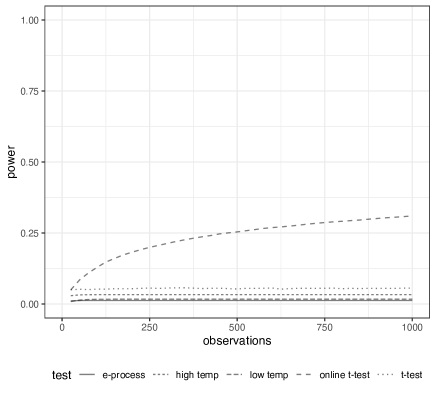
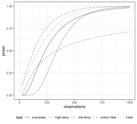
Figure 1: Estimated size (left) and power (right) curves over the number of observations at $\alpha=.05$, for the $t$-test, our sphericity vs. normality likelihood ratio (with $m=.15$) $e$-process , impatience $\kappa\in\{.5,1,2\}$ (‘low impatience’, ‘$e$-process’, ‘high impatience’), and an ‘invalid’ version of the $t$-test (‘online $t$-test’) that rejects as soon as the $p$-value dips under the level $\alpha=.05$. The left plot is for $m=0$ and the right plot for $m=.15$. Both are based on 10 000 simulations and a batch size of 25.

8.2 Case-control experiment and learning the alternative

In this simulation study, we consider a hypothetical case-control experiment, where units are assigned to each case uniformly at random. In each interval of time, we receive the outcomes of a number of treated and control units, where the number of both units is Poisson distributed with parameter $\theta>0$ with minimum of 1. We will assume that the outcomes of the treated units are $\mathcal{N}(\mu_{t},1)$-distributed and the outcomes of the controls are $\mathcal{N}(\mu_{c},1)$-distributed. As a batch of data, we will consider the combined observations of both the treated and control units that arrived in the previous interval of time.

As a result, a batch $X_{i}$ of $n$ outcomes, consisting of $n_{t}$ treated and $n_{c}$ control units, can be represented as

$$X_{i}\sim\begin{bmatrix}1_{n_{t}}m_{t}\\ 1_{n_{c}}m_{c}\end{bmatrix}+\mathcal{N}\left(0,I\right),$$

where $1_{n_{t}}$ and $1_{n_{c}}$ denote a vector of $n_{t}$ and $n_{c}$ ones, respectively, where the first $n_{t}$ elements correspond to the treated units, without loss of generality.

For our simulations, we consider the arrival of 40 batches with $\theta=25$. Without loss of generality, we choose $m_{c}=0$ and $m_{t}=.25$.

We use our $e$-process based on the likelihood ratio for testing exchangeability against $\mathcal{N}_{n}(\overline{1}_{n}\theta,I)$, with $\overline{1}_{n}=(1_{n_{t}},-1_{n_{c}})$, where we consider two options for $\theta$. As a first option, we choose $\theta=m_{t}-m_{c}$, and so behave as if we know the true alternative. As the other option, for the $i$th batch, we set $\theta$ equal to a treatment effect estimator based on all the past batches (excluding the $i$th batch), namely the difference between the sample mean of the treated and sample mean of the control units. Moreover, we consider impatience values $\kappa\in\{.5,1,2\}$. We estimate the normalization constant by using 100 permutations drawn uniformly at random with replacement.

In Figure 2, we report proportion of tests that have been rejected up until each point in time at level $\alpha=0.05$ for various impatience values. The plot on the left features the situation where the alternative is known, and the plot on the right the situation where the alternative is learnt. We see that learning the parameter costs some power, but that the power loss is not enormous. The impatience parameter works as expected in both settings, though its impact seems more dramatic when the parameter is learnt.

We made similar plots to verify the size control and all tests considered controlled size.

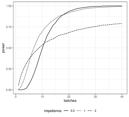
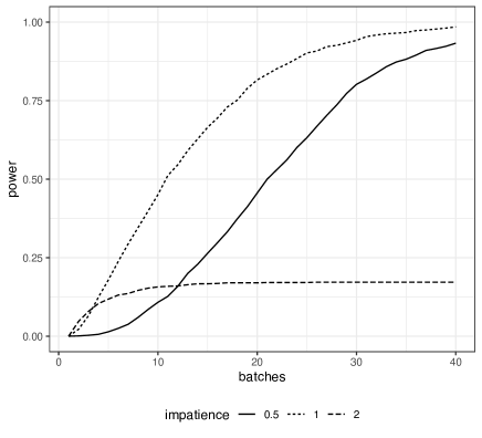
Figure 2: Proportion of tests that rejected so-far at each moment against the number of observed batches at $\alpha=0.05$, with $\mu_{c}=0$ and $\mu_{t}=0.2$, and impatience parameter $\kappa\in 2^{\{-1,0,1\}}$. In the plot on the left the alternative is known, and in the plot on the right the alternative is estimated based on the previously observed data. Both plots are based on 1 000 simulations. The number of treatment and control units in each batch are Poisson distributed with parameter $\theta=25$.

8.3 Testing symmetry and a comparison to de la Peña (1999)

In this section, we consider testing sign-symmetric data as in Section 6.6. We compare our $e$-process to the one by de la Peña (1999), when testing against a simple normal alternative $X_{i}\sim\mathcal{N}(m,1)$.

The power of both processes is plotted in Figure 3, where we use $m=.15$ in the left plot and $m=1$ in the right plot. Notice that our $e$-process is far more powerful. This coincides with the observation of Ramdas et al. (2022a) that the $e$-process of de la Peña (1999) is inadmissible.

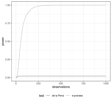
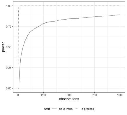
Figure 3: Proportion of tests that rejected so-far at each moment against the number of observed batches at $\alpha=0.05$, for both the de la Peña (1999) $e$-value and ours. The plot on the left is for $m=.15$ and the plot on the right for $m=1$.

9 Acknowledgements

We would like to thank Sam van Meer, Muriel Perez-Ortiz, Tyron Lardy, Will Hartog, Yaniv Romano, Jake Soloff, Stan Koobs, Peter Grünwald, Wouter Koolen and Aaditya Ramdas for useful discussions and comments. Part of this research was performed while the author was visiting the Institute for Mathematical and Statistical Innovation (IMSI), which is supported by the National Science Foundation (Grant No. DMS-1929348).

Appendix A Example: LR for exchangeability

In this section, we discuss a toy example of permutations on a small and finite sample space. While not as statistically interesting as the examples in Section 6, it is more tangible as the group itself is finite and easy to understand.

A.1 Exchangeability on a finite sample space

Suppose our sample space $\mathcal{Y}$ consists of the vectors $[1,2,3]$, $[1,1,2]$ and all their permutations. As a group $\mathcal{G}$, we consider the permutations on 3 elements, which we will denote by $\{abc,acb,bac,bca,cab,cba\}$. For example, $bac$ represents the permutation that swaps the first two elements.

The orbits are then given by all permutations of $[1,2,3]$ and $[1,1,2]$

$$O_{[1,1,2]}=\{[1,1,2],[1,2,1],[2,1,1]\},$$

and

$$O_{[1,2,3]}=\{[1,2,3],[1,3,2],[2,1,3],[2,3,1],[3,1,2],[3,2,1]\}.$$

As $\mathcal{Y}$-valued orbit representatives, we pick the unique element in the orbit that is sorted in ascending order: $[1,1,2]$ and $[1,2,3]$. Notice that the group action of $\mathcal{G}$ is free on $O_{[1,2,3]}$ but not free on $O_{[1,1,2]}$.

For simplicity, let us restrict ourselves to $O_{[1,2,3]}$ first. On this orbit, the map $\gamma$ is defined as the unique permutation that brings the element $[1,2,3]$ to $z\in O_{[1,2,3]}$. Moreover, on this orbit, the null hypothesis then states that $\gamma(Y)$ is uniform on the permutations, which in this case is equivalent to the hypothesis that $Y$ is uniform on $O_{[1,2,3]}$.

Now let us restrict ourselves to $O_{[1,1,2]}$. On this orbit, there are multiple permutations that may bring a given element back to $[1,1,2]$. For example, both $bac$, as well as the identity permutation $abc$ bring $[1,1,2]$ to itself. More generally, any permutation that brings $[1,1,2]$ to $z\in O_{[1,1,2]}$, can be preceded by $bac$, and the result still brings $[1,1,2]$ to $z\in O_{[1,1,2]}$. Even more abstractly speaking, let $\mathcal{S}_{[y]}=\{G\in\mathcal{G}:G[y]=[y]\}$ be the stabilizer subgroup of $[y]$ (the subgroup that leaves $[y]$ unchanged). Then, if $G^{*}\in\mathcal{G}$ carries $[y]$ to $y$, so does any element of $G^{*}\mathcal{S}_{[y]}$.

To construct $\gamma$ on $O_{[1,1,2]}$, let $\overline{S}_{[y]}$ denote a uniform distribution on $\{abc,bac\}$, which is also well-defined in the general case as $\mathcal{S}_{[y]}$ is a compact subgroup and so admits a Haar probability measure. Moreover, let $G_{y}$ be an arbitrary permutation that carries $[y]$ to $y$, say $G_{[1,1,2]}=abc$, $G_{[1,2,1]}=acb$ and $G_{[2,1,1]}=cba$. Then, we define $\gamma(y)=G_{y}\overline{S}_{[y]}$. Concretely, this means that $\gamma([1,1,2])\sim\text{Unif}(abc,bac)$, $\gamma([1,2,1])\sim\text{Unif}(acb,bca)$ and $\gamma([2,1,1])\sim\text{Unif}(cba,cab)$. If $Y$ is indeed uniform on $O_{[1,1,2]}$, then $G_{Y}$ is uniform on $\{abc,acb,cba\}$ and so $\gamma(Y)$ is uniform on $\mathcal{G}$.

The definition of $\gamma$ on the sample space $\mathcal{Y}=O_{[1,2,3]}\cup O_{[1,1,2]}$ is obtained by combining the definitions on the two separate orbits.

A.2 Likelihood ratios

We start with the orbit $O_{[1,2,3]}$. Suppose that our alternative distribution $P_{\mathcal{Y}}^{1}$ conditional on $O_{[1,2,3]}$ is that $Y$ is uniform on $\{[1,2,3],[1,3,2]\}$ and all other arrangements happen with probability 0. As a density on $O_{[1,2,3]}$, we find

$$\begin{cases}0.5,\text{ if }y\in\{[1,2,3],[1,3,2]\},\\ 0,\text{ otherwise}.\end{cases}$$

As the density under the null is $1/6$ for each arrangement, the likelihood ratio is given by

$$\begin{cases}3,\text{ if }y\in\{[1,2,3],[1,3,2]\},\\ 0,\text{ otherwise}.\end{cases}$$

Since the group action is free on the orbit $O_{[1,2,3]}$, $\gamma$ is a bijection between $O_{[1,2,3]}$ and the group, so likelihood ratio is

$$\begin{cases}3,\text{ if }G\in\{abc,acb\},\\ 0,\text{ otherwise}.\end{cases}$$

Now let us consider the orbit $O_{[1,1,2]}$. Suppose that our alternative $P_{\mathcal{Y}}^{1}$ conditional on $O_{[1,1,2]}$ is that $Y$ equals $[1,1,2]$ with probability 1. The likelihood ratio on our orbit then becomes

$$\begin{cases}3,\text{ if }y=[1,1,2],\\ 0,\text{ otherwise}.\end{cases}$$

In this case, the group action is not free, as both $abc$ and $bac$ are permutations that carry $[1,1,2]$ to itself. As a consequence $\gamma([1,1,2])\sim\text{Unif}(abc,bac)$. This induces the following likelihood ratio on $\mathcal{G}$:

$$\begin{cases}3,\text{ if }G\in\{abc,bac\},\\ 0,\text{ otherwise}.\end{cases}$$

Now let us consider a likelihood ratio on $\mathcal{Y}$. For this, it is insufficient that we have an alternative on both $O_{[1,2,3]}$ and $O_{[1,1,2]}$, separately. We need to additionally specify the probability that that $Y$ lands in $O_{[1,2,3]}$ and $O_{[1,1,2]}$ under the alternative. For simplicity, let us assume that the probability of each orbit is 1/2. The likelihood ratio on $\mathcal{Y}$ can then be derived to be

$$\begin{cases}3/2,&\text{ if }y\in\{[1,2,3],[3,2,1],[1,1,2]\},\\ 0,&\text{ otherwise}.\end{cases}$$

The likelihood ratio this induces on $\mathcal{G}$ is

$$\begin{cases}3/2,&\text{ if }G\in\{abc,bac\},\\ 3,&\text{ if }G=abc,\\ 0,&\text{ otherwise},\end{cases}$$

which is exactly the weighted average of the likelihood ratios on $\mathcal{G}$ that were induced on the individual orbits, weighted by the probability of each orbit.

Appendix B Finding the normalization constant analytically

For the likelihood ratio in Sections 6.2 and 6.3, we can easily compute the normalization constant under sphericity. The key trick is to use the fact that $\iota^{\prime}\overline{G}y/\|y\|_{2}$ follows a Beta$(\frac{d-1}{2},\frac{d-1}{2})$ distribution on the interval $[-1,1]$. The normalization constant is then equal to its moment generating function:

$$\mathbb{E}_{\overline{G}}\exp(\mu\iota^{\prime}\overline{G}y)=1+\mu\|y\|_{2}\mathbb{E}_{\overline{G}}\widetilde{B}+\mu^{2}\|y\|_{2}^{2}\mathbb{E}_{\overline{G}}\widetilde{B}^{2}/2!+\dots,$$

where $\widetilde{B}\sim\text{Beta}\left(\frac{d-1}{2},\frac{d-1}{2}\right)$ on $[-1,1]$. For this generalized beta distribution, the odd moments are all 0, since it is symmetric about 0. Moreover, the even moments are given by

$$\mathbb{E}_{\overline{G}}(\widetilde{B})^{k+2}=\mathbb{E}_{\overline{G}}(\widetilde{B})^{k}(k-1)/(n+k-2),$$

with $\mathbb{E}_{\overline{G}}(\widetilde{B})^{0}=1$ and $n$ the dimension of $y$. This means the normalization constant can be easily approximated to high precision, which we exploit in our simulation studies.

Furthermore, it is possible to numerically stabilize the computations by using the fact that

$$1/n\sum_{i}^{n}Z_{i}=\max_{i}\log(Z_{i})+\log(1/n\sum_{i=1}^{n}(\exp(\log(Z_{i})-\max_{i}\log(Z_{i}))))$$

Appendix C Omitted proofs

C.1 Proof of Lemma 1

Proof.

We start with showing that $\mathcal{S}^{h}(y)$ is a subgroup, then we show it is closed, so that by the compactness of $\mathcal{G}$ it is also compact.

First observe that the identity element is in $\mathcal{S}^{h}(y)$. Suppose that $S_{1},S_{2}\in\mathcal{S}^{h}(y)$. Then,

$$h(S_{1}S_{2}y)=h(S_{2}y)=h(y),$$

so that $\mathcal{S}^{h}(y)$ is closed under compositions. Moreover, it is closed under inverses as for any $S\in\mathcal{S}^{h}(y)$

$$h(y)=h(Iy)=h(SS^{-1}y)=h(S^{-1}y).$$

Hence, $\mathcal{S}^{h}(y)$ is a subgroup of $\mathcal{G}$.

Finally, we show that $\mathcal{S}^{h}(y)$ is topologically closed. Define the map $f_{y}:\mathcal{G}\to\mathcal{Y}$ as the composition between $h$ and the group action: $f_{y}(G)=h(Gy)$. As both $h$ and the group action are continuous, the composition $f_{y}$ is also continuous. Since the space in which $\{h(y)\}$ lives is Hausdorff, it is also a $T_{1}$ space so that $\{h(y)\}$ is closed. Hence, $\mathcal{S}^{h}(y)$ is the pre-image of the closed set $\{h(y)\}$ under a continuous map, and so $\mathcal{S}^{h}(y)$ is also closed, and therefore compact. ∎

C.2 Proof of Theorem 1

Proof.

Let us start by fixing an arbitrary orbit $O$ under $\mathcal{G}$ acting on $\mathcal{Y}$.

As $Y$ is $\mathcal{G}$ invariant, it is also invariant under any of its compact subgroups. By Lemma 1, $\mathcal{S}$ is such a compact subgroup. As a consequence, $Y$ is uniform on the (sub)orbits of $\mathcal{S}$ acting on $O$.

Let us condition on the suborbit in which $Y$ falls. This suborbit consists of all the points $y$ for which $h(y)=h(GY)$ for some $G\in\mathcal{G}$. As $\mathcal{G}$ acts transitively on $O$, any point on the suborbit can be reached by applying a transformation $G$ to $Y$. Hence, the suborbit of $Y$ under $\mathcal{S}$ consists exactly of those elements $y\in O$ for which $h(y)=h(Y)$. This is exactly the subset to which we restrict $Y$ by conditioning on $h(Y)$. As a result, the conditional distribution of $Y$ given $O$ and $h(Y)$ is uniform on this suborbit.

This distribution can be characterized as the distribution of $\overline{S}z$, where $\overline{S}$ is uniform on $\mathcal{S}$, and $z$ is some element on the suborbit. ∎

C.3 Proof of Theorem 2

Proof.

We start by showing that every statistic of the type $e_{T_{+}}$ is exact, and then we show that every exact $e$-value can be written as $e_{T_{+}}$ for some statistic $T_{+}$.

To show that every statistic $e_{T_{+}}$ is exact, we first show that this is true on each orbit $O_{y}$, $y\in\mathcal{Y}$. We find

$$\mathbb{E}_{\overline{G}}e_{T_{+}}(\overline{G}y) =\mathbb{E}_{\overline{G}}\frac{{T_{+}}(\overline{G}y)}{\mathbb{E}_{\overline{G}_{2}}{T_{+}}(\overline{G}_{2}\overline{G}y)}$$

$$=\mathbb{E}_{\overline{G}}\frac{{T_{+}}(\overline{G}y)}{\mathbb{E}_{\overline{G}_{2}}{T_{+}}(\overline{G}_{2}y)}$$

$$=\mathbb{E}_{\overline{G}}\frac{{T_{+}}(\overline{G}y)}{\mathbb{E}_{\overline{G}_{2}}{T_{+}}(\overline{G}_{2}y)}$$

$$=\frac{1}{\mathbb{E}_{\overline{G}_{2}}{T_{+}}(\overline{G}_{2}y)}\mathbb{E}_{\overline{G}}{T_{+}}(\overline{G}y)$$

$$=1,$$

where $\overline{G}_{2}$ is independent from $\overline{G}$ and also uniform on $\mathcal{G}$.

As a result, we immediately find that $e_{T_{+}}$ is an exact $e$-value for $\mathcal{G}$ invariance, as for any $\mathcal{G}$ invariance probability measure $P$, we have

$$\mathbb{E}_{Y}^{P}e_{T}(Y)=\mathbb{E}_{Y}^{P}\mathbb{E}_{\overline{G}}e_{T}(\overline{G}Y)=\mathbb{E}_{Y}^{P}1 =1.$$

Next, we show that every exact $e$-value can be written as $e_{T_{+}}$. Suppose that $T_{+}$ itself is an exact $e$-value for $H_{0}^{\mathcal{G}}$. Then,

$$\mathbb{E}_{Y}^{P}{T_{+}}(Y)=\mathbb{E}_{Y}^{P}\mathbb{E}_{\overline{G}}{T_{+}}(\overline{G}Y)=1,$$

for any distribution $P$ in $H_{0}^{\mathcal{G}}$. In particular, it is true if we choose $Y\sim\delta_{y}$ for any $y\in\mathcal{Y}$, where $\delta_{y}$ denotes the Dirac measure at $y$. As a consequence, ${T_{+}}(Y)$ is an exact $e$-value for $H_{0}^{\mathcal{G}}$ on every orbit

$$\mathbb{E}_{Y}^{\delta_{y}}\mathbb{E}_{\overline{G}}{T_{+}}(\overline{G}Y)=\mathbb{E}_{\overline{G}}{T_{+}}(\overline{G}y)=1.$$

Now, as $\mathbb{E}_{\overline{G}}{T_{+}}(\overline{G}y)=1$, we have

$$e_{T_{+}}(y)=\frac{{T_{+}}(y)}{\mathbb{E}_{\overline{G}}{T_{+}}(\overline{G}y)}={T_{+}}(y).$$

Hence, if ${T_{+}}$ is an exact $e$-value for $H_{0}^{\mathcal{G}}$, then it must be equal to some test statistic of the form $e_{T_{+}}$.

For the second claim, it suffices to observe that if an $e$-value is valid but not exact, then we can improve its power by adding a sufficiently small deterministic constant so that it is still valid. ∎

C.4 Proof of Theorem 3

Proof.

Conditionally on $X_{[1:n)}$, we have that $X_{[1:n]}$ is $\mathcal{S}_{n}$ invariant: $X_{[1:n]}\overset{d}{=}\overline{S}_{n}^{2}X_{[1:n]}$, where $\overline{S}_{n}^{2}$ is independent from $X_{[1:n]}$ and uniform on $\mathcal{S}_{n}$. As a consequence,

$$\mathbb{E}_{X_{[1:n]}}\left[\frac{T_{n}(X_{[1:n]})}{\mathbb{E}_{\overline{S}_{n}}T_{n}(\overline{S}_{n}X_{[1:n]})}\right] =\mathbb{E}_{\overline{S}_{n}^{2}X_{[1:n]}}\left[\frac{T_{n}(X_{[1:n]})}{\mathbb{E}_{\overline{S}_{n}}T_{n}(\overline{S}_{n}\overline{S}_{n}^{2}X_{[1:n]})}\right]$$

$$=\mathbb{E}_{X_{[1:n]}}\left(\mathbb{E}_{\overline{S}_{n}^{2}}\left[\frac{T_{n}(\overline{S}_{n}^{2}X_{[1:n]})}{\mathbb{E}_{\overline{G}_{n}}T_{n}(\overline{S}_{n}\overline{S}_{n}^{2}X_{[1:n]})}\right]\right)$$

$$=\mathbb{E}_{X_{[1:n]}}\left(\mathbb{E}_{\overline{S}_{n}^{2}}\left[\frac{T_{n}(\overline{S}_{n}^{2}X_{[1:n]})}{\mathbb{E}_{\overline{S}_{n}}T_{n}(\overline{S}_{n}X_{[1:n]})}\right]\right)$$

$$=\mathbb{E}_{X_{[1:n]}}\left(\frac{\mathbb{E}_{\overline{S}_{n}^{2}}T_{n}(\overline{S}_{n}^{2}X_{[1:n]})}{\mathbb{E}_{\overline{S}_{n}}T_{n}(\overline{S}_{n}X_{[1:n]})}\right)$$

$$=\mathbb{E}_{X_{[1:n]}}1=1,$$

where the second equality follows from Tonelli’s theorem and the third equality from the fact that $\overline{S}_{n}S\overset{d}{=}\overline{S}_{n}$ for any $S\in\mathcal{S}_{n}$, as $\overline{S}_{n}$ is $\mathcal{S}_{n}$ invariant. This means that $e_{n}(X_{[1:n]})$ is an exact $e$-value conditional on $X_{[1:n)}$. Moreover, $e_{1}(X_{1})$ is a ‘plain’ exact $e$-value as $\mathcal{S}_{1}=\mathcal{G}_{1}$. Applying the law of iterated expectations, we have

$$\mathbb{E}e_{n}(X_{[1:n]}) =\mathbb{E}\left[\prod_{i=1}^{n}\frac{T_{i}(X_{[1:i]})}{\mathbb{E}_{\overline{S}_{i}}T_{i}(\overline{S}_{i}X_{[1:i]})}\right]$$

$$=\mathbb{E}\left[\mathbb{E}\left(\frac{T_{n}(X_{[1:n]})}{\mathbb{E}_{\overline{S}_{n}}T_{n}(\overline{S}_{n}X_{[1:n]})}\prod_{i=1}^{n-1}\frac{T_{i}(X_{[1:i]})}{\mathbb{E}_{\overline{S}_{i}}T_{i}(\overline{S}_{i}X_{[1:i]})}\Bigm{|}X_{[1:n)}\right)\right]$$

$$=\mathbb{E}\left[\prod_{i=1}^{n-1}\frac{T_{i}(X_{[1:i]})}{\mathbb{E}_{\overline{S}_{i}}T_{i}(\overline{S}_{i}X_{[1:i]})}\mathbb{E}\left(\frac{T_{n}(X_{[1:n]})}{\mathbb{E}_{\overline{S}_{n}}T_{n}(\overline{S}_{n}X_{[1:n]})}\Bigm{|}X_{[1:n)}\right)\right]$$

$$=\mathbb{E}\left[\prod_{i=1}^{n-1}\frac{T_{i}(X_{[1:i]})}{\mathbb{E}_{\overline{S}_{i}}T_{i}(\overline{S}_{i}X_{[1:i]})}\right]$$

$$=\mathbb{E}\left[\frac{T_{1}(X_{1})}{\mathbb{E}_{\overline{G}_{1}}T_{i}(\overline{G}_{1}X_{1})}\right]=1,$$

where the second-to-last equality follows from induction. ∎

C.5 Proof of Theorem 4

Proof.

For notational convenience, let us define a function $f$ as $f(y)=\mathbb{E}_{\overline{G}}d\mathbb{P}_{\mathcal{Y}}/d\lambda(\overline{G}y)$. Observe that $f$ is a $\mathcal{G}$ invariant function as

$$f(Gy)=\mathbb{E}_{\overline{G}}d\mathbb{P}_{\mathcal{Y}}/d\lambda(\overline{G}y)=\mathbb{E}_{\overline{G}}d\mathbb{P}_{\mathcal{Y}}/d\lambda(\overline{G}Gy)=f(y),$$

since $\overline{G}\overset{d}{=}\overline{G}G$ as $\overline{G}$ is a $\mathcal{G}$ invariant random variable. As a consequence, $f$ is constant on the orbit $\{z\in\mathcal{Y}:y=Gz,\text{ for some }G\}$ of $y$. As $0<f(y)<\infty$, the function $f$ is proportional to a uniform distribution on every orbit. Now, the statistic integrates to 1 on every orbit as

$$\mathbb{E}_{\overline{G}_{2}}\frac{d\mathbb{P}_{\mathcal{Y}}/d\lambda(\overline{G}_{2}y)}{\mathbb{E}_{\overline{G}}d\mathbb{P}_{\mathcal{Y}}/d\lambda(\overline{G}\overline{G}_{2}y)}=\mathbb{E}_{\overline{G}_{2}}\frac{d\mathbb{P}_{\mathcal{Y}}/d\lambda(\overline{G}_{2}y)}{\mathbb{E}_{\overline{G}}d\mathbb{P}_{\mathcal{Y}}/d\lambda(\overline{G}y)}=\frac{\mathbb{E}_{\overline{G}_{2}}d\mathbb{P}_{\mathcal{Y}}/d\lambda(\overline{G}_{2}y)}{\mathbb{E}_{\overline{G}}d\mathbb{P}_{\mathcal{Y}}/d\lambda(\overline{G}y)}=1,$$

where $\overline{G}_{2}$ is uniform on $\mathcal{G}$, independently from $\overline{G}$. Hence, for every orbit, the statistic is a likelihood ratio statistic for testing a uniform distribution on an orbit against $\mathbb{P}_{\mathcal{Y}}$. Finally, as $\mathcal{G}$ invariance is equivalent to being uniform on every orbit, the statistic is a likelihood ratio statistic for testing $\mathbb{P}_{\mathcal{Y}}$ against $\mathcal{G}$ invariance. ∎

References

- (1)
- Chiu & Bloem-Reddy (2023) Chiu, K. & Bloem-Reddy, B. (2023), ‘Non-parametric hypothesis tests for distributional group symmetry’, arXiv preprint arXiv:2307.15834 .
- Chung & Fraser (1958) Chung, J. H. & Fraser, D. A. S. (1958), ‘Randomization tests for a multivariate two-sample problem’, Journal of the American Statistical Association 53(283), 729–735.
- de la Peña (1999) de la Peña, V. H. (1999), ‘A general class of exponential inequalities for martingales and ratios’, The Annals of Probability 27(1), 537–564.
- Grünwald et al. (2023) Grünwald, P., de Heide, R. & Koolen, W. (2023), ‘Safe testing’, arXiv preprint arXiv:1906.07801 .
- Ignatiadis et al. (2023) Ignatiadis, N., Wang, R. & Ramdas, A. (2023), ‘E-values as unnormalized weights in multiple testing’, Biometrika p. asad057.
- Johari et al. (2022) Johari, R., Koomen, P., Pekelis, L. & Walsh, D. (2022), ‘Always valid inference: Continuous monitoring of a/b tests’, Operations Research 70(3), 1806–1821.
- Kallenberg (2017) Kallenberg, O. (2017), Random measures, theory and applications, Vol. 1, Springer.
- Kashlak (2022) Kashlak, A. B. (2022), ‘Asymptotic invariance and robustness of randomization tests’, arXiv preprint arXiv:2211.00144 .
- Koning (2023) Koning, N. W. (2023), ‘More power by using fewer permutations’, arXiv preprint arXiv:2307.12832 .
- Koning & Hemerik (2023) Koning, N. W. & Hemerik, J. (2023), ‘More Efficient Exact Group Invariance Testing: using a Representative Subgroup’, Biometrika .
- Koolen & Grünwald (2022) Koolen, W. M. & Grünwald, P. (2022), ‘Log-optimal anytime-valid e-values’, International Journal of Approximate Reasoning 141, 69–82.
- Larsen et al. (2023) Larsen, N., Stallrich, J., Sengupta, S., Deng, A., Kohavi, R. & Stevens, N. (2023), ‘Statistical challenges in online controlled experiments: A review of a/b testing methodology’, arXiv preprint arXiv:2212.11366 .
- Lehmann & Stein (1949) Lehmann, E. L. & Stein, C. (1949), ‘On the theory of some non-parametric hypotheses’, The Annals of Mathematical Statistics 20(1), 28–45.
- Pérez-Ortiz et al. (2022) Pérez-Ortiz, M. F., Lardy, T., de Heide, R. & Grünwald, P. (2022), ‘E-statistics, group invariance and anytime valid testing’, arXiv preprint arXiv:2208.07610 .
- Ramdas et al. (2023) Ramdas, A., Grünwald, P., Vovk, V. & Shafer, G. (2023), ‘Game-theoretic statistics and safe anytime-valid inference’, arXiv preprint arXiv:2210.01948 .
- Ramdas & Manole (2023) Ramdas, A. & Manole, T. (2023), ‘Randomized and exchangeable improvements of markov’s, chebyshev’s and chernoff’s inequalities’, arXiv preprint arXiv:2304.02611 .
- Ramdas et al. (2022a) Ramdas, A., Ruf, J., Larsson, M. & Koolen, W. (2022a), ‘Admissible anytime-valid sequential inference must rely on nonnegative martingales’, arXiv preprint arXiv:2009.03167 .
- Ramdas et al. (2022b) Ramdas, A., Ruf, J., Larsson, M. & Koolen, W. M. (2022b), ‘Testing exchangeability: Fork-convexity, supermartingales and e-processes’, International Journal of Approximate Reasoning 141, 83–109.
- Vovk (2021) Vovk, V. (2021), ‘Testing randomness online’, Statistical Science 36(4), 595–611.
- Wang & Ramdas (2023) Wang, H. & Ramdas, A. (2023), ‘The extended ville’s inequality for nonintegrable nonnegative supermartingales’.
- Wang & Ramdas (2022) Wang, R. & Ramdas, A. (2022), ‘False discovery rate control with e-values’, Journal of the Royal Statistical Society Series B: Statistical Methodology 84(3), 822–852.