Parallel-in-Time Probabilistic Numerical ODE Solvers

Abstract

Probabilistic numerical solvers for ordinary differential equations (ODEs) treat the numerical simulation of dynamical systems as problems of Bayesian state estimation. Aside from producing posterior distributions over ODE solutions and thereby quantifying the numerical approximation error of the method itself, one less-often noted advantage of this formalism is the algorithmic flexibility gained by formulating numerical simulation in the framework of Bayesian filtering and smoothing. In this paper, we leverage this flexibility and build on the time-parallel formulation of iterated extended Kalman smoothers to formulate a parallel-in-time probabilistic numerical ODE solver. Instead of simulating the dynamical system sequentially in time, as done by current probabilistic solvers, the proposed method processes all time steps in parallel and thereby reduces the span cost from linear to logarithmic in the number of time steps. We demonstrate the effectiveness of our approach on a variety of ODEs and compare it to a range of both classic and probabilistic numerical ODE solvers.

Keywords: probabilistic numerics, ordinary differential equations, numerical analysis, parallel-in-time methods, Bayesian filtering and smoothing.

1 Introduction

Ordinary differential equations (ODEs) are used throughout the sciences to describe the evolution of dynamical systems over time. In machine learning, ODEs provide a continuous description of certain neural networks (Chen et al., 2018) and optimization procedures (Helmke et al., 2012; Su et al., 2016), and are used in generative modeling with normalizing flows (Papamakarios et al., 2021) and diffusion models (Song et al., 2021), among others. Unfortunately, all but the simplest ODEs are too complex to be solved analytically. Therefore, numerical methods are required to obtain a solution. While a multitude of numerical solvers has been developed over the last century (Hairer et al., 1993; Deuflhard and Bornemann, 2012; Butcher, 2016), most commonly-used methods do not provide a quantification of their own inevitable numerical approximation error.

Probabilistic numerics provides a framework for treating classic numerical problems as problems of probabilistic inference (Hennig et al., 2015; Oates and Sullivan, 2019; Hennig et al., 2022). In the context of ODEs, methods based on Gaussian process regression (Skilling, 1992; Hennig and Hauberg, 2014) and in particular Gauss–Markov regression (Schober et al., 2019; Kersting et al., 2020; Tronarp et al., 2019) provide an efficient and flexible approach to compute posterior distributions over the solution of ODEs (Bosch et al., 2021; Krämer and Hennig, 2020), and even partial differential equations (Krämer et al., 2022) and differential-algebraic equations (Bosch et al., 2022). These so-called ODE filters typically scale cubically in the ODE dimension (as do most implicit ODE solvers) and specific approximations enable linear scaling (shared by most explicit solvers) (Krämer et al., 2022). But to date, their linear scaling with the number of time steps remains.

For very large-scale simulations with very long time horizons, the sequential processing in time of most ODE solvers can become a bottleneck. This motivates the development of parallel-in-time methods: By leveraging the ever-increasing parallelization capabilities of modern computer hardware, parallel-in-time methods can achieve sub-linear scaling in the number of time steps (Gander, 2015). One well-known method of this kind is Parareal (Lions et al., 2001). It achieves temporal parallelism by combining an expensive, accurate solver with a cheap, coarse solver, in such a way that the fine solver is only ever applied to individual time slices in a parallel manner, leading to a square-root scaling (in ideal conditions). But, due to its sequential coarse-grid solve, Parareal still has only limited concurrency (Gander and Vandewalle, 2007), and while it has recently been extended probabilistically by Pentland et al. (2021, 2022) to improve its performance and convergence, these methods do not provide probabilistic solutions to ODEs per se.

In this paper, we leverage the time-parallel formulation of Gaussian filters and smoothers (Särkkä and García-Fernández, 2021; Yaghoobi et al., 2021, 2023) to formulate a parallel-in-time probabilistic numerical ODE solver. The paper is structured as follows. Section 2 formulates numerical ODE solutions as Bayesian state estimation problems and presents the established, sequential, filtering-based probabilistic ODE solvers. Section 3 then presents our proposed parallel-in-time probabilistic ODE solver; first as exact inference for affine ODEs, then as an iterative, approximate algorithm for general nonlinear ODEs. Section 4 then presents experiments on a variety of ODEs and compares the performance of our proposed method to that of existing, both probabilistic and non-probabilistic, ODE solvers. Finally, Section 5 concludes with a discussion of our results and an outlook on future work.

2 Numerical ODE Solutions as Bayesian State Estimation

Consider an initial value problem (IVP) of the form

$$\dot{y}(t)=f(y(t),t),\quad t\in[0,T],\qquad y(0)=y_{0},$$ (1)

with vector field $f:\mathbb{R}^{d}\times\mathbb{R}\to\mathbb{R}^{d}$ and initial value $y_{0}\in\mathbb{R}^{d}$. To capture the numerical error that arises from temporal discretization, the quantity of interest in probabilistic numerics for ODEs is the probabilistic numerical ODE solution, defined as

$$p\left(y(t)~{}\Big{|}~{}y(0)=y_{0},\left\{\dot{y}(t_{n})=f(y(t_{n}),t_{n})\right\}_{n=1}^{N}\right),$$ (2)

for some prior $p\left(y(t)\right)$ and with $\{t_{n}\}_{n=1}^{N}\subset[0,T]$ the chosen time-discretisation.

In the following, we pose the probabilistic numerical ODE solution as a problem of Bayesian state estimation, and we define the prior, likelihood, data, and approximate inference scheme. For a more detailed description of the transformation of an IVP into a Gauss–Markov regression problem, refer to Tronarp et al. (2019).

2.1 Gauss–Markov Process Prior

We model the solution $y$ of the IVP with a $\nu$-times integrated Wiener process prior (IWP($\nu$)). More precisely, let $Y(t)=\left[Y^{(0)}(t),Y^{(1)}(t),\dots,Y^{(\nu)}(t)\right]$ be the solution of the following linear, time-invariant stochastic differential equation with Gaussian initial condition

$$\,\text{d}Y^{(i)}(t) =Y^{(i+1)}(t)\,\text{d}t,\qquad i=0,\dots,\nu-1,$$ (3a)

$$\,\text{d}Y^{(\nu)}(t) =\Gamma\,\text{d}W(t),$$ (3b)

$$Y(0) \sim\mathcal{N}\left(\mu_{0},\Sigma_{0}\right),$$ (3c)

with initial mean and covariance $\mu_{0}\in\mathbb{R}^{d(\nu+1)}$, $\Sigma_{0}\in\mathbb{R}^{d(\nu+1)\times d(\nu+1)}$, diffusion $\Gamma\in\mathbb{R}^{d\times d}$, and $d$-dimensional Wiener process $W:\mathbb{R}\to\mathbb{R}^{d}$. Then, $Y^{(i)}$ is chosen to model the $i$-th derivative of the IVP solution $y$. By construction, accessing the $i$-th derivative can be done by multiplying the state $Y$ with a projection matrix $E_{i}\coloneqq I_{d}\otimes e_{i}$, that is, $Y^{(i)}(t)=E_{i}Y(t)$.

This continuous-time prior satisfies discrete transition densities (Särkkä and Solin, 2019)

$$Y(t+h)\mid Y(t)\sim\mathcal{N}\left(\Phi(h)Y(t),Q(h)\right),$$ (4)

with transition matrix and process noise covariance $\Phi(h),Q(h)\in\mathbb{R}^{d(\nu+1)\times d(\nu+1)}$ and step $h\in\mathbb{R}_{+}$. For the IWP($\nu$) these can be computed in closed form (Kersting et al., 2020), as

$$\Phi(h) =I_{d}\otimes\breve{\Phi}(h), \left[\breve{\Phi}(h)\right]_{ij} =\mathbbm{1}_{i=j}\frac{h^{i-j}}{(j-i)!},$$ (5a)

$$Q(h) =I_{d}\otimes\breve{Q}(h), \left[\breve{Q}(h)\right]_{ij} =\frac{h^{2\eta+1-i-j}}{(2\nu+1-i-j)(\nu-i)!(\nu-j)!}.$$ (5b)

Remark 1 (Alternative Gauss–Markov priors).

While $\nu$-times integrated Wiener process priors have been the most common choice for filtering-based probabilistic ODE solvers in recent years, the methodology is not limited to this choice. Alternatives include the $\nu$-times integrated Ornstein–Uhlenbeck process and the class of Matérn processes, both of which have a similar continuous-time SDE representation as well as Gaussian transition densities in discrete time. Refer to Tronarp et al. (2021) and Särkkä and Solin (2019).

The initial distribution $\mathcal{N}(\mu_{0},\Sigma_{0})$ is chosen such that it encodes the initial condition $y(0)=y_{0}$. Furthermore, to improve the numerical stability and the quality of the posterior, we initialize not only on the function value $Y^{(0)}(0)=y_{0}$, but also the higher order derivatives, that is, $Y^{(i)}(0)=\frac{\,\text{d}^{i}y}{\,\text{d}t^{i}}(0)$ for all $i\leq\nu$ (Krämer and Hennig, 2020). These terms can be efficiently computed via Taylor-mode automatic differentiation (Griewank, 2000; Bettencourt et al., 2019). As a result, we obtain an initial distribution with mean

$$\mu_{0}=\left[y_{0},\frac{\,\text{d}y}{\,\text{d}t}(0),\dots,\frac{\,\text{d}^{\nu}y}{\,\text{d}t^{\nu}}(0)\right]^{T},$$ (6)

and zero covariance $\Sigma_{0}=0$, since the initial condition has to hold exactly.

2.2 Observation Model and Data

To relate the introduced Gauss–Markov prior to the IVP problem from Equation 1, we define an observation model in terms of the information operator

$$\mathcal{Z}[y](t)\coloneqq\dot{y}(t)-f\left(y(t),t\right).$$ (7)

By construction, $\mathcal{Z}$ maps the true IVP solution $y$ exactly to the zero function, that is, $\mathcal{Z}[y]\equiv 0$. In terms of the continuous process $Y$, the information operator can be expressed as

$$\mathcal{Z}[Y](t)=E_{1}Y(t)-f\left(E_{0}Y(t),t\right),$$ (8)

where $E_{0}$ and $E_{1}$ are the projection matrices introduced in Section 2.1 which select the zeroth and first derivative from the process $Y$, respectively. There again, if $Y$ corresponds to the true IVP solution (and its true derivatives), then $\mathcal{Z}[Y]\equiv 0$.

Conversely, inferring the true IVP solution requires conditioning the process $Y(t)$ on $Z(t)=0$ over the whole continuous interval $t\in[0,T]$. Since this is in general intractable, we instead condition $Y(t)$ only on discrete observations $Z(t_{n})=0$ on a grid $\mathbb{T}=\{t_{n}\}_{n=1}^{N}$. This leads to the Dirac likelihood model commonly used in ODE filtering (Tronarp et al., 2019):

$$Z(t_{n})\mid Y(t_{n})\sim\delta\left(Y^{(1)}(t_{n})-f\left(Y^{(0)}(t_{n}),t_{n}\right)\right),$$ (9)

with zero-valued data $Z(t_{n})=0$ for all $t_{n}\in\mathbb{T}$.

Remark 2 (Information operators for other differential equation problems).

Similar information operators can be defined for other types of differential equations that are not exactly of the first-order form as given in Equation 1, such as higher-order differential equations, Hamiltonian dynamics, or differential-algebraic equations (Bosch et al., 2022).

2.3 Discrete-Time Inference Problem

The combination of prior, likelihood, and data results in a Bayesian state estimation problem

$$Y(0) \sim\mathcal{N}\left(\mu_{o},\Sigma_{0}\right),$$ (10a)

$$Y(t_{n+1})\mid Y(t_{n}) \sim\mathcal{N}\left(\Phi(t_{n+1}-t_{n})Y(t_{n}),Q(t_{n+1}-t_{n})\right),$$ (10b)

$$Z(t_{n})\mid Y(t_{n}) \sim\delta\left(Y^{(1)}(t_{n})-f\left(Y^{(0)}(t_{n}),t_{n}\right)\right),$$ (10c)

with zero data $Z(t_{n})=0$ for all $t_{n}\in\mathbb{T}$. The posterior distribution over $Y^{(0)}(t)$ then provides a probabilistic numerical ODE solution to the given IVP, as formulated in Equation 2.

This is a standard nonlinear Gauss–Markov regression problem, for which many approximate inference algorithms have previously been studied (Särkkä and Svensson, 2023). In the context of probabilistic ODE solvers, a popular approach for efficient approximate inference is Gaussian filtering and smoothing, where the solution is approximated with Gaussian distributions

$$p\left(Y(t)\mid\{Z(t_{n})=0\}_{n=1}^{N}\right)\approx\mathcal{N}\left(\mu(t),\Sigma(t)\right).$$ (11)

This is most commonly performed with extended Kalman filtering (EKF) and smoothing (EKS) (Schober et al., 2019; Tronarp et al., 2019; Kersting et al., 2020); though other methods have been proposed, for example based on numerical quadrature (Kersting and Hennig, 2016) or particle filtering (Tronarp et al., 2019). Iterated extended Kalman smoothing (e.g. Bell, 1994; Särkkä and Svensson, 2023) computes the “maximum a posteriori” estimate of the probabilistic numerical ODE solution (Tronarp et al., 2021). This will be the basis for the parallel-in-time ODE filter proposed in this work, explained in detail in Section 3.

2.4 Practical Considerations for Probabilistic Numerical ODE Solvers

While Bayesian state estimation methods such as the extended Kalman filter and smoother can, in principle, be directly applied to the formulated state estimation problem, there are a number of modifications and practical considerations that should be taken into account:

• Square-root formulation: Gaussian filters often suffer from numerical stability issues when applied to the ODE inference problem defined in Equation 10, in particular when using high orders and small steps. To alleviate these issues, probabilistic numerical ODE solvers are typically formulated in square-root form (Krämer and Hennig, 2020); this is also the case for the proposed parallel-in-time method.

• Preconditioned state transitions: Krämer and Hennig (2020) suggest a coordinate change preconditioner to make the state transition matrices step-size independent and thereby improve the numerical stability of EKF-based probabilistic ODE solvers. This preconditioner is also used in this work.

• Uncertainty calibration: The Gauss–Markov prior as introduced in Section 2.1 has a free parameter, the diffusion $\Gamma$, which directly influences the uncertainty estimates returned by the ODE filter. In this paper, we consider scalar diffusions $\Gamma=\sigma\cdot I$ and compute a quasi-maximum likelihood estimate for the parameter $\sigma$ post-hoc, as suggested by Tronarp et al. (2019).

• Approximate linearization: Variants of the standard EKF/EKS-based inference have been proposed in which the linearization of the vector-field is done only approximately. Approximating the Jacobian of the ODE vector field with zero enables inference with a complexity which scales only linearly with the ODE dimension (Krämer et al., 2022), while still providing polynomial convergence rates (Kersting et al., 2020). A diagonal approximation of the Jacobian preserves the linear complexity, but improves the stability properties of the solver (Krämer et al., 2022). In this work, we only consider the exact first-order Taylor linearization.

• Local error estimation and step-size adaptation: Rather than predefining the time discretization grid, certain solvers employ an adaptive approach where the solver dynamically constructs the grid while controlling an internal estimate of the numerical error. Step-size adaptation based on local error estimates have been proposed for both classic (Hairer et al., 1993, Chapter II.4) and probabilistic ODE solvers (Schober et al., 2019; Bosch et al., 2021). On the other hand, global step-size selection is often employed in numerical boundary value problem (BVP) solvers (Ascher et al., 1995, Chapter 9), and has been extended to filtering-based probabilistic BVP solvers (Krämer and Hennig, 2021). For our purposes, we will focus on fixed grids.

3 Parallel-in-Time Probabilistic Numerical ODE Solvers

This section develops the main method proposed in this paper: a parallel-in-time probabilistic numerical ODE solver.

3.1 Parallel-Time Exact Inference in Affine Vector Fields

Let us first consider the simple case: An initial value problem with affine vector field

$$\dot{y}(t)=L(t)y(t)+d(t),\quad t\in[0,T],\qquad y(0)=y_{0}.$$ (12)

The corresponding information model of the probabilistic solver is then also affine, with

$$Z(t)\mid Y(t) \sim\delta\left(H(t)Y(t)-d(t)\right),$$ (13a)

$$H(t) \coloneqq E_{1}-L(t)E_{0}.$$ (13b)

Let $\mathbb{T}=\{t_{n}\}_{n=1}^{N}\subset[0,T]$ be a discrete time grid. To simplify the notation in the following, we will denote a function evaluated at time $t_{n}$ by a subscript $n$, that is $Y(t_{n})=:Y_{n}$, except for the transition matrices where we will use $\Phi_{n}\coloneqq\Phi(t_{n+1}-t_{n})$ and $Q_{n}\coloneqq Q(t_{n+1}-t_{n})$. Then, the Bayesian state estimation problem from Equation 10 reduces to inference of $Y(t)$ in the model

$$Y_{0} \sim\mathcal{N}\left(\mu_{o},\Sigma_{0}\right),$$ (14a)

$$Y_{n+1}\mid Y_{n} \sim\mathcal{N}\left(\Phi_{n}Y_{n},Q_{n}\right),$$ (14b)

$$Z_{n}\mid Y_{n} \sim\delta\left(H_{n}Y_{n}-d_{n}\right),$$ (14c)

with zero data $Z_{n}=0$ for all $n=1,\dots,N$. Since this is an affine Gaussian state estimation problem, it can be solved exactly with Gaussian filtering and smoothing (Kalman, 1960; Rauch et al., 1965; Särkkä and Svensson, 2023); see also (Tronarp et al., 2019, 2021) for explicit discussions of probabilistic numerical solvers for affine ODEs.

Recently, Särkkä and García-Fernández (2021) presented a parallel-time formulation of Bayesian filtering and smoothing, as well as a concrete algorithm for exact linear Gaussian filtering and smoothing—which could be directly applied to the problem formulation in Equation 14. But as mentioned in • ‣ Section 2.4, the resulting ODE solver might suffer from numerical instabilities. Therefore, we use the square-root formulation of the parallel-time linear Gaussian filter and smoother by Yaghoobi et al. (2023). In the following, we review the details of the algorithm.

3.1.1 Parallel-Time General Bayesian Filtering and Smoothing

First, we follow the presentation of Särkkä and García-Fernández (2021) and formulate Bayesian filtering and smoothing as prefix sums. We define elements $a_{n}=(f_{n},g_{n})$ with

$$f_{n}(Y_{n}\mid Y_{n-1}) =p(Y_{n}\mid Z_{n},Y_{n-1}),$$ (15a)

$$g_{n}(Y_{n-1}) =p(Z_{n}\mid Y_{n-1}),$$ (15b)

where for $n=1$ we have $p(Y_{1}\mid Z_{1},Y_{0})=p(Y_{1}\mid Z_{1})$ and $p(Z_{1}\mid Y_{0})=p(Z_{1})$, together with a binary operator $\otimes_{f}:(f_{i},g_{i})\otimes_{f}(f_{j},g_{j})\mapsto(f_{ij},g_{ij})$ defined by

$$f_{ij}(x\mid z) \coloneqq\frac{\int g_{j}(y)f_{j}(x\mid y)f_{i}(y\mid z)\,\text{d}y}{\int g_{j}(y)f_{i}(y\mid z)\,\text{d}y},$$ (16a)

$$g_{ij}(z) \coloneqq g_{i}(z)\int g_{j}(y)f_{i}(y\mid z)\,\text{d}y.$$ (16b)

Then, Särkkä and García-Fernández (2021, Theorem 3) show that $\otimes_{f}$ is associative and that

$$a_{1}\otimes_{f}\dots\otimes_{f}a_{n}=\begin{bmatrix}p(Y_{n}\mid Z_{1:n})\\ p(Z_{1:n})\end{bmatrix},$$ (17)

that is, the filtering marginals and the marginal likelihood of the observations at step $n$ are the results of a cumulative sum of the elements $a_{1:n}$ under $\otimes_{f}$. Since the operator $\otimes_{f}$ is associative, this quantity can be computed in parallel with prefix-sum algorithms, such as the parallel scan algorithm by Blelloch (1989).

Remark 3 (On Prefix-Sums).

Prefix sums, also known as cumulative sums or inclusive scans, play an important role in parallel computing. Their computation can be efficiently parallelized and, if enough parallel resources are available, their (span) computational cost can be reduced from linear to logarithmic in the number of elements. One such algorithm is the well-known parallel scan algorithm by Blelloch (1989) which, given $N$ elements and $N/2$ processors, computes the prefix sum in $2\lceil\log_{2}N\rceil$ sequential steps with $2N-2$ invocations of the binary operation. This algorithm is implemented in both tensorflow (Abadi et al., 2015) and JAX (Bradbury et al., 2018); the latter is used in this work.

The time-parallel smoothing step can be constructed similarly: We define elements $b_{n}=p(Y_{n}\mid Z_{1:n},Y_{n+1})$, with $b_{N}=p(Y_{N}\mid Z_{1:N})$, and a binary operator $b_{i}\otimes_{s}b_{j}=b_{ij}$, with

$$b_{ij}(x\mid z) =\int b_{i}(x\mid y)b_{j}(y\mid z)\,\text{d}y.$$ (18)

Then, $\otimes_{s}$ is associative and the smoothing marginal at time step $n$ is the result of a reverse cumulative sum of the elements $b_{n:N}$ under $\otimes_{s}$ (Särkkä and García-Fernández, 2021):

$$b_{n}\otimes_{s}\dots\otimes_{s}b_{N}=p(Y_{n}\mid Z_{1:N}).$$ (19)

Again, since the smoothing operator $\otimes_{s}$ is associative, this cumulative sum can be computed in parallel with a prefix-sum algorithm (Blelloch, 1989).

3.1.2 Parallel-Time Linear Gaussian Filtering in Square-Root Form

In the linear Gaussian case, the filtering elements $a_{n}=(f_{n},g_{n})$ can be parameterized by a set of parameters $\{A_{n},b_{n},C_{n},\eta_{n},J_{n}\}$ as follows:

$$f_{n}(Y_{n}\mid Y_{n-1}) =p(Y_{n}\mid Z_{n},Y_{n-1})=\mathcal{N}\left(Y_{n};A_{n}Y_{n-1}+b_{n},C_{n}\right),$$ (20a)

$$g_{n}(Y_{n-1}) =p(Z_{n}\mid Y_{n-1})\propto\mathcal{N}_{I}\left(Y_{n-1};\eta_{n},J_{n}\right),$$ (20b)

where $\mathcal{N}_{I}$ denotes a Gaussian density parameterized in information form, that is, $\mathcal{N}_{I}(x;\eta,J)=\mathcal{N}(x;J^{-1}\eta,J^{-1})$. The parameters $\{A_{n},b_{n},C_{n},\eta_{n},J_{n}\}$ can be computed explicitly from the given state-space model (Särkkä and García-Fernández, 2021, Lemma 7). But since probabilistic numerical ODE solvers require a numerically stable implementation of the underlying filtering and smoothing algorithm (Krämer and Hennig, 2020), we formulate the parallel-time linear Gaussian filtering algorithm in square-root form, following Yaghoobi et al. (2023).

To this end, let $\sqrt{M}$ denote a left square-root of a positive semi-definite matrix $M$, that is, $\sqrt{M}\sqrt{M}^{T}=M$; the matrix $\sqrt{M}$ is sometimes also called a “generalised Cholesky factor” of $M$ (S. Grewal and P. Andrews, 2014). To operate on square-root matrices, we also define the triangularization operator: Given a wide matrix $M\in\mathbb{R}^{n\times m}$, $m\geq n$, the triangularization operator $\operatorname{tria}(M)$ first computes the QR decomposition of $M^{\mathsf{T}}$, that is, $M^{\mathsf{T}}=QR$, with wide orthonormal $Q\in\mathbb{R}^{m\times n}$ and square upper-triangular $R\in\mathbb{R}^{n\times n}$, and then returns $R^{\mathsf{T}}$. This operator plays a central role in square-root filtering algorithms as it enables the numerically stable addition of covariance matrices, provided square-roots are available: Given two positive semi-definite matrices $A,B\in\mathbb{R}^{n\times n}$ with square-roots $\sqrt{A},\sqrt{B}$, a square-root of the sum $A+B$ can be computed as

$$\sqrt{A+B}=\operatorname{tria}\left(\begin{bmatrix}\sqrt{A}&\sqrt{B}\end{bmatrix}\right).$$ (21)

With these definitions in place, we briefly review the parallel-time linear Gaussian filtering algorithm in square-root form as provided by Yaghoobi et al. (2023) in the following.

Parameterization of the filtering elements.

Let $m_{0}=\mu_{0}$, $P_{0}=\Sigma_{0}$, and $m_{n}=0$, $P_{n}=0$ for all $n\geq 1$, and define

$$m_{n}^{-} =\Phi_{n-1}m_{n-1},$$ (22a)

$$\sqrt{P_{n}^{-}} =\operatorname{tria}\left(\begin{bmatrix}\Phi_{n-1}\sqrt{P_{n-1}}&\sqrt{Q_{n-1}}\end{bmatrix}\right).$$ (22b)

Then, the square-root parameterization of the filtering elements $a_{n}$ is given by

$$A_{n} =(I-K_{n}H_{n})\Phi_{n-1},$$ (23a)

$$b_{n} =m_{n}^{-}-K_{n}\left(H_{n}m_{n}^{-}-d_{n}\right),$$ (23b)

$$\sqrt{C_{n}} =\Psi_{22},$$ (23c)

$$\eta_{n} =\sqrt{J_{n}}\sqrt{S_{n}}^{-1}d_{n},$$ (23d)

$$\sqrt{J_{n}} =\Phi_{n-1}^{\mathsf{T}}H_{n}^{\mathsf{T}}\sqrt{S_{n}}^{-\mathsf{T}},$$ (23e)

where $I$ is the identity matrix and $\Psi_{22}$, $\sqrt{S_{n}}$ and $K_{n}$ are defined via

$$\begin{bmatrix}\Psi_{11}&0\\ \Psi_{21}&\Psi_{22}\end{bmatrix} =\operatorname{tria}\left(\begin{bmatrix}H_{n}\sqrt{P_{n}^{-}}&\sqrt{R_{n}}\\ \sqrt{P_{n}^{-}}&0\end{bmatrix}\right),$$ (24a)

$$\sqrt{S_{n}} =\Psi_{11},$$ (24b)

$$K_{n} =\Psi_{21}\Psi_{11}^{-1}.$$ (24c)

For generality the formula includes an observation noise covariance $R_{n}$, but note that in the context of probabilistic ODE solvers we have a noiseless measurement model with $\sqrt{R_{n}}=0$.

Associative filtering operator.

Let $a_{i},a_{j}$ be two filtering elements, parameterized in square-root form by $a_{i}=\{A_{i},b_{i},\sqrt{C_{i}},\eta_{i},\sqrt{J_{i}}\}$ and $a_{j}=\{A_{j},b_{j},\sqrt{C_{j}},\eta_{j},\sqrt{J_{j}}\}$. Then, the associative filtering operator $\otimes_{f}$ computes the filtering element $a_{ij}=a_{i}\otimes_{f}a_{j}$ as

$$A_{ij} =A_{j}A_{i}-A_{j}\sqrt{C_{i}}\Xi_{11}^{-\mathsf{T}}\Xi_{21}^{\mathsf{T}}A_{i},$$ (25a)

$$b_{ij} =A_{j}\left(I-\sqrt{C_{i}}\Xi_{11}^{-\mathsf{T}}\Xi_{21}^{\mathsf{T}}\right)(b_{i}+\sqrt{C_{i}}\sqrt{C_{i}}^{\mathsf{T}}\eta_{j})+b_{j},$$ (25b)

$$\sqrt{C_{ij}} =\operatorname{tria}\left(\begin{bmatrix}A_{j}\sqrt{C_{i}}\Xi_{11}^{-\mathsf{T}}&\sqrt{C_{j}}\end{bmatrix}\right),$$ (25c)

$$\eta_{ij} =A_{i}^{\mathsf{T}}\left(I-\Xi_{21}\Xi_{11}^{-1}\sqrt{C_{i}}^{\mathsf{T}}\right)\left(\eta_{j}-\sqrt{J_{j}}\sqrt{J_{j}}^{\mathsf{T}}b_{i}\right)+\eta_{i},$$ (25d)

$$\sqrt{J_{ij}} =\operatorname{tria}\left(\begin{bmatrix}A_{i}^{\mathsf{T}}\Xi_{22}&\sqrt{J_{i}}\end{bmatrix}\right),$$ (25e)

where $\Xi_{11}$, $\Xi_{21}$, $\Xi_{22}$ are defined via

$$\begin{bmatrix}\Xi_{11}&0\\ \Xi_{21}&\Xi_{22}\end{bmatrix}=\operatorname{tria}\left(\begin{bmatrix}\sqrt{C_{i}}^{\mathsf{T}}\sqrt{J_{j}}&I\\ \sqrt{J_{j}}&0\end{bmatrix}\right).$$ (26)

See Yaghoobi et al. (2023) for the detailed derivation.

The filtering marginals.

The filtering marginals are then given by

$$p(Y_{n}|Z_{1:n})=\mathcal{N}\left(Y_{n};m_{n}^{f},P_{n}^{f}\right),\qquad\text{with}\qquad m_{n}^{f}\coloneqq b_{1:n},\quad\sqrt{P_{n}^{f}}\coloneqq\sqrt{C_{1:n}}.$$ (27)

This concludes the parallel-time linear Gaussian square-root filter.

3.1.3 Parallel-Time Linear Gaussian Smoothing in Square-Root Form

Similarly to the filtering equations, the linear Gaussian smoothing can also be formulated in terms of smoothing elements $b_{n}$ and an associative operator $\otimes_{s}$, and the smoothing marginals can also be computed with a parallel prefix-sum algorithm.

Parameterization of the smoothing elements.

The smoothing elements $b_{n}$ can be described by a set of parameters $\{E_{n},g_{n},\sqrt{L_{n}}\}$, as

$$b_{n}=p(Y_{n}\mid Z_{1:n},Y_{n+1})=\mathcal{N}\left(Y_{n};E_{n}Y_{n+1}+g_{n},\sqrt{L_{n}}\sqrt{L_{n}}^{\mathsf{T}}\right).$$ (28)

The smoothing element parameters can be computed as

$$E_{n} =\Pi_{21}\Pi_{11}^{-1},$$ (29a)

$$g_{n} =m_{n}^{f}-E_{n}\Phi_{n}m_{n}^{f},$$ (29b)

$$\sqrt{L_{n}} =\Pi_{22},$$ (29c)

where $I$ is the identity matrix and the matrices $\Pi_{11}$, $\Pi_{21}$, $\Pi_{22}$ are defined via

$$\begin{bmatrix}\Pi_{11}&0\\ \Pi_{21}&\Pi_{22}\end{bmatrix}=\operatorname{tria}\left(\begin{bmatrix}\Phi_{n}\sqrt{P_{n}^{f}}&\sqrt{Q_{n}}\\ \sqrt{P_{n}^{f}}&0\end{bmatrix}\right).$$ (30)

Associative smoothing operator.

Given two smoothing elements $b_{i},b_{j}$ be two filtering elements, parameterized in square-root form by $b_{i}=\{E_{i},g_{i},\sqrt{L_{i}}\}$ and $b_{j}=\{E_{j},g_{j},\sqrt{L_{j}}\}$, the associative smoothing operator $\otimes_{s}$ computes the smoothing element $b_{ij}=b_{i}\otimes_{s}b_{j}$ as

$$E_{ij} =E_{i}E_{j},$$ (31a)

$$g_{ij} =E_{i}g_{j}+g_{i},$$ (31b)

$$\sqrt{L_{ij}} =\operatorname{tria}\left(\begin{bmatrix}E_{i}\sqrt{L_{j}}&\sqrt{L_{i}}\end{bmatrix}\right).$$ (31c)

The smoothing marginals.

The smoothing marginals can then be retrieved from the reverse cumulative sum of the smoothing elements as

$$p(Y_{n}\mid Z_{1:N}) =\mathcal{N}\left(Y_{n};m_{n}^{s},P_{n}^{s}\right),$$ (32a)

$$m_{n}^{s} =g_{n:N},$$ (32b)

$$\sqrt{P_{n}^{s}} =\sqrt{L_{n:N}}.$$ (32c)

Refer to Yaghoobi et al. (2023) for a thorough derivation. The full parallel-time Rauch–Tung–Striebel smoother is summarized in Algorithm 1.

Algorithm 1 Parallel-time Rauch–Tung–Striebel Smoother (ParRTS)

1:Initial distribution $(\mu_{0},\Sigma_{0})$, linear transition models $\{(\Phi_{n},Q_{n})\}_{n=1}^{N}$, affine observation models $\{(H_{n},d_{n})\}_{n=1}^{N}$, data $Z_{1:N}$.

2:Compute the filtering elements:

3:$a_{n}=(A_{n},b_{n},\sqrt{C_{n}},\eta_{n},\sqrt{J_{n}})$ for all $n=1,\dots,N$ $\triangleright$ Eq. (23)

4:Run the time-parallel Kalman filter:

5:$\left\{\left(A_{n}^{f},b_{n}^{f},\sqrt{C_{n}^{f}},\eta_{n}^{f},\sqrt{J_{n}^{f}}\right)\right\}_{n=1}^{N}\leftarrow\texttt{AssociativeScan}\left(\otimes_{f},(a_{n})_{n=1}^{N}\right)$ $\triangleright$ Eq. (25)

6:$p\left(Y_{n}\mid Z_{1:N}\right)=\mathcal{N}\left(Y_{n};\mu_{n}^{f},\Sigma_{n}^{f}\right)\leftarrow\mathcal{N}\left(Y_{n};b_{n}^{f},C_{n}^{f}\right)$ $\triangleright$ Filtering marginals

7:Compute the smoothing elements:

8:$b_{n}=(E_{n},g_{n},\sqrt{L_{n}})$ for all $n=0,\dots,N$ $\triangleright$ Eq. (28)

9:Run the time-parallel Rauch–Tung–Striebel smoother:

10:$\left\{\left(E_{n}^{s},g_{n}^{s},\sqrt{L_{n}^{s}}\right)\right\}_{n=1}^{N}\leftarrow\texttt{ReverseAssociativeScan}\left(\otimes_{s},(b_{n})_{n=1}^{N}\right)$ $\triangleright$ Eq. (31)

11:Smoothing marginals $p(Y_{n}\mid Z_{1:N})=\mathcal{N}\left(Y_{n};g_{n}^{s},L_{n}^{s}\right)$

This concludes the parallel-in-time probabilistic numerical ODE solver for affine ODEs: since affine ODEs result in state-estimation problems with affine state-space models, as discussed in the beginning of this section, the parallel-time Rauch–Tung–Striebel smoother presented here can be used to solve affine ODEs in parallel time.

3.2 Parallel-Time Approximate Inference in Nonlinear Vector Fields

Let us now consider the general case: An IVP with nonlinear vector field

$$\dot{y}(t)=f(y(t),t),\quad t\in[0,T],\qquad y(0)=y_{0}.$$ (33)

As established in Section 2, the corresponding state estimation problem is

$$Y_{0} \sim\mathcal{N}\left(\mu_{o},\Sigma_{0}\right),$$ (34a)

$$Y_{n+1}\mid Y_{n} \sim\mathcal{N}\left(\Phi_{n}Y_{n},Q_{n}\right),$$ (34b)

$$Z_{n}\mid Y_{n} \sim\delta\left(E_{1}Y_{n}-f\left(E_{0}Y_{n},t_{n}\right)\right),$$ (34c)

with temporal discretization $\mathbb{T}=\{t_{n}\}_{n=1}^{N}\subset[0,T]$ and zero data $Z_{n}=0$ for all $n=1,\dots,N$. In this section, we describe a parallel-in-time algorithm for solving this state estimation problem: the iterated extended Kalman smoother (IEKS).

3.2.1 Globally Linearizing the State-Space Model

To make inference tractable, we will linearize the whole state-space model along a reference trajectory. And since the observation model (specified in Equation 34c) is the only nonlinear part of the state-space model, it is the only part that requires linearization. In this paper, we only consider linearization with a first-order Taylor expansion, but other methods are possible; see Remarks 4 and 5.

For any time-point $t_{n}\in\mathbb{T}$, we approximate the nonlinear observation model

$$Z_{n}\mid Y_{n}\sim\delta\left(E_{1}Y_{n}-f\left(E_{0}Y_{n},t_{n}\right)\right)$$ (35)

with an affine observation model by performing a first-order Taylor series expansion around a linearization point $\eta_{n}\in\mathbb{R}^{d(\nu+1)}$. We obtain the affine model

$$Z_{n}\mid Y_{n}\sim\delta\left(H_{n}Y_{n}-d_{n}\right),$$ (36)

with $H_{n}$ and $d_{n}$ defined as

$$H_{n} \coloneqq E_{1}-F_{y}(E_{0}\eta_{n},t_{n})E_{0},$$ (37a)

$$d_{n} \coloneqq f(E_{0}\eta_{n},t_{n})-F_{y}(E_{0}\eta_{n},t_{n})E_{0}\eta_{n},$$ (37b)

where $F_{y}$ denotes the Jacobian of $f$ with respect to $y$.

In the IEKS, this linearization is performed globally on all time steps simultaneously along a trajectory of linearization points $\left\{\eta_{n}\right\}_{n=1}^{N}\subset\mathbb{R}^{d(\nu+1)}$. We obtain the following linearized inference problem:

$$Y_{0} \sim\mathcal{N}\left(\mu_{o},\Sigma_{0}\right),$$ (38a)

$$Y_{n+1}\mid Y_{n} \sim\mathcal{N}\left(\Phi_{n}Y_{n},Q_{n}\right),$$ (38b)

$$Z_{n}\mid Y_{n} \sim\delta\left(H_{n}Y_{n}-d_{n}\right),$$ (38c)

with zero data $Z_{n}=0$ for all $n=1,\dots,N$. This is now a linear state-space model with linear Gaussian observations. It can therefore be solved exactly with the numerically stable, time-parallel Kalman filter and smoother presented in Section 3.1.

Remark 4 (Linearizing with approximate Jacobians (EK0 & DiagonalEK1)).

To reduce the computational complexity with respect to the state dimension of the ODE, the vector field can also be linearized with an approximate Jacobian. Established choices include $F_{y}\approx 0$ and $F_{y}\approx\operatorname{diag}(\nabla_{y}f)$, which result in probabilistic ODE solvers known as the EK0 and DiagonalEK1, respectively. See Krämer et al. (2022) for more details.

Remark 5 (Statistical linear regression).

Statistical linear regression (SLR) is a more general framework for approximating conditional distributions with affine Gaussian distributions, and many well-established filters can be understood as special cases of SLR. This includes notably the Taylor series expansion used in the EKF/EKS, but also sigma-point methods such as the unscented Kalman filter and smoother (Julier et al., 2000; Julier and Uhlmann, 2004; Särkkä, 2008), and more. For more information on SLR-based filters and smoothers refer to Särkkä and Svensson (2023, Chapter 9).

3.2.2 Iterated Extended Kalman Smoothing

The IEKS (Bell, 1994; Särkkä and Svensson, 2023) is an approximate Gaussian inference method for nonlinear state-space models, which iterates between linearizing the state-space model along the current best-guess trajectory and computing a new state trajectory estimate by solving the linearized model exactly. It can equivalently also be seen as an efficient implementation of the Gauss–Newton method, applied to maximizing the posterior density of the state trajectory (Bell, 1994). This also implies that the IEKS computes not just some Gaussian estimate, but the maximum a posteriori (MAP) estimate of the state trajectory. In the context of probabilistic numerical ODE solvers, the IEKS has been previously explored by Tronarp et al. (2021), and the resulting MAP estimate has been shown to satisfy polynomial convergence rates to the true ODE solution. Here, we formulate an IEKS-based probabilistic ODE solver in a parallel-in-time manner, by exploiting the time-parallel formulation of the Kalman filter and smoother from Section 3.1.

The IEKS is an iterative algorithm, which starts with an initial guess of the state trajectory and then iterates between the following two steps:

1. Linearization step: Linearize the state-space model along the current best-guess trajectory. This can be done independently for each time step and is therefore fully parallelizable.

2. Linear smoothing step: Solve the resulting linear state-space model exactly with the time-parallel Kalman filter and smoother from Section 3.1.

The algorithm terminates when a stopping criterion is met, for example when the change in the MAP estimate between two iterations is sufficiently small. A pseudo-code summary of the method is provided in Algorithm 2.

Algorithm 2 IEKS-based Parallel-in-Time Probabilistic ODE Solver

1:ODE-IVP $(f,y_{0})$, prior transition model $\left\{(\Phi_{n},Q_{n})\right\}_{n=1}^{N}$, time grid $\left\{t_{n}\right\}_{n=0}^{N}\subset[0,T]$.

2:$\mu_{0}\leftarrow\texttt{ComputeExactInitialState}(f,y_{0})$ $\triangleright$ With automatic differentiation

3:$\Sigma_{0}\leftarrow 0$

4:$\eta_{n}\leftarrow\mu_{0}$ for all $n=0,\dots,N$ $\triangleright$ Constant initial guess of state trajectory

5:while stopping criterion not met do

6:     for $n=1,\dots,N$ do $\triangleright$ Can be done fully in parallel

7:         $H_{n},d_{n}\leftarrow\texttt{LinearizeObservationModel}(f,\eta_{n},t_{n})$ $\triangleright$ As in Sec. 3.2.1

8:     end for

9:     $\left\{\mu_{n},\Sigma_{n}\right\}_{n=1}^{N}\leftarrow\texttt{ParRTS}\left((\mu_{o},\Sigma_{0}),\{(\Phi_{n},Q_{n})\}_{n=1}^{N},\{(H_{n},d_{n})\}_{n=1}^{N}\right)$ $\triangleright$ As in Sec. 3.1

10:     $\eta_{n}\leftarrow\mu_{n}$ for all $n=1,\dots,N$

11:end while

12:$y(t_{n})\sim\mathcal{N}\left(E_{0}\mu_{n},E_{0}\Sigma_{n}E_{0}^{\mathsf{T}}\right)$ for $n=1,\dots,N$.

As with the sequential filtering-based probabilistic ODE solvers as presented in Section 2, the mean and covariance of the initial distribution $Y(0)\sim\mathcal{N}\left(\mu_{0},\Sigma_{0}\right)$ are chosen such that $\mu_{0}$ corresponds to the exact solution of the ODE and its derivatives and $\Sigma_{0}$ is set to zero; see also Krämer and Hennig (2020). The initial state trajectory estimate $\{\eta_{n}\}_{n=0}^{N}$ is chosen to be constant, that is, $\eta_{n}=\mu_{0}$ for all $n=0,\dots,N$. Note that since only $E_{0}\eta_{n}$ is required to perform the linearization, it could equivalently be set to $\eta_{n}=[y_{0},0,\dots,0]$ for all $n$.

Finally, the stopping criterion should be chosen such that the algorithm terminates when the MAP estimate of the state trajectory has converged. In our experiments, we chose a combination of two criteria: (i) the change in the state trajectory estimate between two iterations is sufficiently small, or (ii) the change in the objective value between two iterations is sufficiently small, where the objective value is defined as the negative log-density of the state trajectory:

$$\mathcal{V}(\eta_{0:N})=\frac{1}{2}\sum_{n=1}^{N}\left\|\eta_{n}-\Phi(h_{n})\eta_{n-1}\right\|_{Q^{-1}(h)}^{2}.$$ (39)

In our experiments, we use a relative tolerance of $10^{-13}$ for the first criterion and absolute and relative tolerances of $10^{-9}$ and $10^{-6}$ for the second criterion, respectively.

3.3 Computational Complexity of the Time-Parallel Probabilistic ODE Solver

The standard, sequential formulation of a Kalman smoother has a computational cost that scales linearly in the number of data points $N$, of the form

$$C_{\text{KS}}^{s}=N\cdot\left(C_{\text{predict}}^{s}+C_{\text{update}}^{s}+C_{\text{smooth}}^{s}\right),$$ (40)

where $C_{\text{predict}}^{s},C_{\text{update}}^{s},C_{\text{smooth}}^{s}$ are the costs of the sequential formulation of the predict, update, and smoothing steps, respectively. For nonlinear models, the extended Kalman filter/smoother linearizes the observation model sequentially at each prediction mean. With $C_{\text{linearize}}$ the cost of linearization, which requires evaluating the vector field and computing its Jacobian, the cost for a sequential extended Kalman smoother becomes

$$C_{\text{EKS}}^{s}=N\cdot\left(C_{\text{predict}}^{s}+C_{\text{linearize}}+C_{\text{update}}^{s}+C_{\text{smooth}}^{s}\right).$$ (41)

The proposed IEKS differs in two ways: (i) the prefix-sum formulation of the Kalman smoother enables a time-parallel inference with logarithmic complexity, and (ii) the linearization is not done locally in a sequential manner but can be performed globally, fully in parallel. Assuming a large enough number of processors / threads, the span cost of a single parallelized IEKS iteration becomes

$$C_{\text{EKS}}^{p}=C_{\text{linearize}}+\log(N)\cdot\left(C_{\text{filter}}^{p}+C_{\text{smooth}}^{p}\right),$$ (42)

where $C_{\text{filter}}^{p},C_{\text{smooth}}^{p}$ are the costs of the associative filtering and smoothing operation as used in the parallel Kalman filter formulation, respectively. They differ from the costs of the sequential formulation in a constant manner.

4 Experiments

This section investigates the utility and performance of the proposed parallel IEKS-based ODE filter on a range of experiments. It is structured as follows: First, Section 4.1 investigates the runtime of a single IEKS step in its sequential and parallel formulation, over a range of grid sizes and for different GPUs. Section 4.2 then compares the performance of both ODE solver implementations on multiple test problems. Finally, Section 4.3 benchmarks the proposed method against other well-established ODE solvers, including both classic and probabilistic numerical methods.

Implementation

All experiments are implemented in the Python programming language with the JAX software framework (Bradbury et al., 2018). Reference solutions are computed with SciPy (Virtanen et al., 2020) and Diffrax (Kidger, 2021). Unless specified otherwise, experiments are run on an NVIDIA V100 GPU. Code for the implementation and experiments is publicly available on GitHub.

4.1 Runtime of a Single Extended Kalman Smoother Step

We first evaluate the runtime of the proposed method for only a single IEKS iteration, which consists of one linearization of the model along a trajectory and one extended Kalman smoother step. To this end, we consider the logistic ordinary differential equation

$$\dot{y}(t)=y(t)\left(1-y(t)\right),\qquad t\in[0,10],\qquad y(0)=0.01;$$ (43)

though, since here we only investigate the runtime of a single IEKS iteration and thus do not actually solve the problem by iteratively re-linearizing, the precise choice of ODE is not very important. We then compare the runtime of the sequential and parallel EKS formulation for different grid sizes, resulting from time discretizations with step sizes $h=2^{0},2^{1},\dots,2^{14}$, and for multiple GPUs with varying numbers of CUDA cores. Figure 1 shows the results.

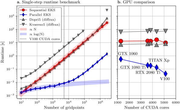
Figure 1: The parallel EKS shows logarithmic scaling and benefits from GPU improvements. In comparison, the sequential EKS and the classic Dopri5 and Kvaerno5 solvers show the expected linear runtime complexity (left). They also do not show relevant changes in runtime for GPUs with higher numbers of CUDA cores (right).

First, we observe the expected logarithmic scaling of the parallel EKS with respect to the grid size, for grids of size up to around $\sim 5\cdot 10^{3}$ (Figure 1a). For larger grid sizes the runtime of the parallel EKS starts to grow linearly. This behaviour is expected: The NVIDIA V100 GPU used in this experiment has only 5120 CUDA cores, so for larger grids the filter and smoother pass can not be fully parallelized anymore and additional grid points need to be processed sequentially. But, the overall runtime of the parallel EKS is still significantly lower than the runtime of the sequential EKS throughout all grid sizes.

Figure 1b. shows runtimes for different GPUs with varying numbers of CUDA cores for a grid of size $N=81920$. We observe that both the sequential EKS, as well as the classic Dopri5 and Kvaerno5 solvers (Dormand and Prince, 1980; Shampine, 1986; Kværnø, 2004), do not show a benefit from the improved GPU hardware. This is expected as these methods do not explicitly aim to leverage parallelizaton. On the other hand, the runtime of the parallel EKS decreases as the number of CUDA cores increases, and we observe speed-ups of up to an order of magnitude by using a different GPU. Be reminded once more that these evaluations only considered a single IEKS step, so they do not show the runtimes for computing the actual probabilistic numerical ODE solutions—these will be the subject of interest in the next sections.

4.2 The Parallel-IEKS ODE Filter Compared to its Sequential Version

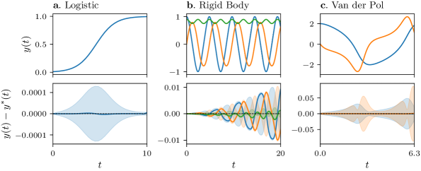
Figure 2: Trajectories, errors, and error estimates computed by the parallel-in-time solver. Top row: ODE solution trajectories. Visually, all three test problems seem to be solved accurately. Bottom row: Numerical errors (lines) and error estimates (shaded area). Ideally, for good calibration, the error should be of similar magnitude than the error estimate. The posterior appears underconfident on the logistic and Van der Pol ODE, and reasonably confident for the rigid body problem.

In this experiment we compare the proposed parallel-in-time ODE solver to a probabilistic solver based on the sequential implementation of the IEKS. In addition to the logistic ODE as introduced in Equation 43, we consider two more problems: An initial value problem based on the rigid body dynamics (Hairer et al., 1993)

$$\dot{y}(t)=\begin{bmatrix}-2y_{2}(t)y_{3}(t)\\ 1.25y_{1}(t)y_{3}(t)\\ -0.5y_{1}(t)y_{2}(t)\end{bmatrix},\qquad t\in[0,20],\qquad y(0)=\begin{bmatrix}1\\ 0\\ 0.9\end{bmatrix},$$ (44)

and the Van der Pol oscillator (Van der Pol, 1920)

$$\dot{y}(t)=\begin{bmatrix}y_{2}(t)\\ \mu\left(\left(1-y_{1}(t)^{2}\right)y_{2}(t)-y_{1}(t)\right)\end{bmatrix},\qquad t\in[0,6.3],\qquad y(0)=\begin{bmatrix}2\\ 0\end{bmatrix},$$ (45)

here in a non-stiff version with parameter $\mu=1$.

We first solve the three problems with the parallel IEKS on grids of sizes $30$, $200$, and $100$, respectively for the logistic, rigid body, and Van der Pol problem, with a two-times integrated Wiener process prior. Reference solutions are computed with diffrax’s Kvaerno5 solver using adaptive steps and very low tolerances $\tau_{\{\text{abs},\text{rel}\}}=10^{-12}$ (Kidger, 2021; Kværnø, 2004). Figure 2 shows the resulting solution trajectories, together with numerical errors and error estimates. For these grid sizes, the parallel IEKS computes accurate solutions on all three problems. Regarding calibration, the posterior appears underconfident for the logistic and Van der Pol problems as it overestimates the numerical error by more than one order of magnitude. This is likely not due to the proposed method itself as underconfidence of ODE filters in low-error regimes has been previously observed (Bosch et al., 2021). For the rigid body problem, the posterior appears reasonably confident and the error estimate is of similar magnitude as the numerical error.

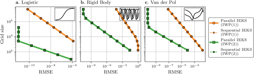
Figure 3: The sequential and parallel IEKS compute numerically identical solutions. For all three problems and all considered grid sizes, the sequential and parallel IEKS achieve (numerically) identical errors. This is expected, as both versions compute the same quantities and only differ in their implementation.

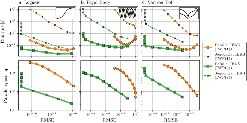
Figure 4: Work-precision diagrams for the sequential and parallel IEKS-based ODE solver. Top row: Runtime in seconds per error (lower-left is better). Bottom row: Speed-up of the parallel over the sequential IEKS (higher is better). Accross all problems, grid sizes, and priors, the parallel IEKS outperforms the sequential IEKS.

Next, we investigate the performance of the parallel IEKS and compare it to its sequential implementation. We solve the three problems with the parallel and sequential IEKS on a range of grid sizes, with both a one- and two-times integrated Wiener process prior. Reference solutions are computed with diffrax’s Kvaerno5 solver using adaptive steps and very low tolerances ($\tau_{\text{abs}}=10^{-16},\tau_{\text{rel}}=10^{-13}$). Figure 3 shows the achieved root-mean-square errors (RMSE) for different grid sizes in a work-precision diagram. As expected, both the parallel and the sequential IEKS always achieve the same error for each problem and grid size, as both versions compute the same quantities and only differ in their implementation. However, the methods differ significantly in actual runtime, as shown in Figure 4. In our experiments on an NVIDIA V100 GPU, the parallel IEKS is always strictly faster than the sequential implementation across all problems, grid sizes, and priors, and we observe speed-ups of multiple orders of magnitude. Thus, when working with a GPU, the parallel IEKS appears to be strictly superior to the sequential IEKS.

4.3 Benchmarking the Parallel-IEKS ODE Filter

Finally, we compare the proposed method to a range of well-established ODE solvers, including both classic and probabilistic numerical methods: we compare against the implicit Euler method, the Kvaerno3 (KV3) and Kvaerno5 (KV5) solvers (Kværnø, 2004) provided by Diffrax (Kidger, 2021), as well as the sequential EKS with local linearization, which is one of the currently most popular probabilistic ODE solvers. Note that since the IEKS is considered to be an implicit solver (Tronarp et al., 2021), we only compare to other implicit and semi-implicit methods, and therefore neither include explicit Runge–Kutta methods nor the EKS with zeroth order linearization (also known as EK0) in our comparison. Reference solutions are computed with diffrax’s Kvaerno5 solver with adaptive steps and a very low error tolerance setting ($\tau_{\text{abs}}=10^{-16},\tau_{\text{rel}}=10^{-13}$).

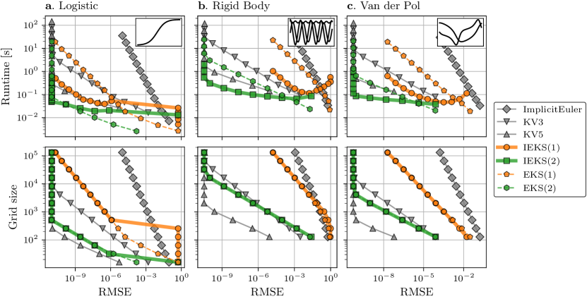
Figure 5: Benchmarking the parallel IEKS against other common numerical ODE solvers. Top row: Work-precision diagrams showing runtimes per error for a range of different ODE solvers (lower-left is better). Bottom row: Errors per specified grid size (lower-left is better). Per grid size, the closely related EKS and IEKS solvers often coincide; KV5 achieves the lowest error per step as it has the highest order. In terms of runtime, the IEKS outperforms both the EKS and KV5 on medium-to-high accuracy settings due to its logarithmic time complexity.

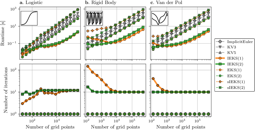
Figure 6: Runtimes of the ODE solvers for each grid size, and number of IEKS iterations. While all sequential solvers demonstrate linear scaling with the number of grid points, the parallel IEKS shows sub-linear scaling up to a certain grid size (top). The number of IEKS iterations until convergence can vary with the grid size and the problem, but it seems that in many cases ~$10$ iterations suffice (bottom). The sequential methods solve the ODE in one sweep.

Figure 5 shows the results as work-precision diagrams. For small grid sizes (low accuracy), the logarithmic time complexity of the parallel IEKS seems to not be very relevant and the IEKS is outperformed by the non-iterated EKS. In the particular case of the logistic ODE, it further seems that the MAP estimate differs significantly from ODE solution and thus the error on coarse grids is high (lower left figure). However, for larger grid sizes (medium-to-high accuracy), the parallel IEKS outperforms both its sequential, non-iterated counterpart, as well as the classic methods. In particular, the parallel IEKS with IWP(2) prior often shows runtimes lower than those of the classic KV5 method, even though it has a lower order of convergence and is an iterative method; see also Figure 6 for runtimes per grid size and for the number of iterations performed by the IEKS. Overall, the logarithmic time complexity of the proposed parallel IEKS appears to be very beneficial for high accuracy settings on GPUs and makes the parallel IEKS a very competitive ODE solver in this comparison.

5 Conclusion

In this work, we have developed a parallel-in-time probabilistic numerical ODE solver. The method builds on iterated extended Kalman smoothing to compute the maximum a posteriori estimate of the probabilistic ODE solution, and by using the time-parallel formulation of the IEKS it is able to efficiently leverage modern parallel computer hardware such as GPUs to parallelize its computations. Given enough processors or cores, the proposed algorithm shares the logarithmic cost per time step of the parallel IEKS and the underlying parallel prefix-sum algorithm, as opposed to the linear time complexity of standard, sequentially-operating ODE solvers. We evaluated the performance of the proposed method in a number of experiments, and have seen that the proposed parallel-in-time solver can provide speed-ups of multiple orders of magnitude over the sequential IEKS-based solver. We also compared the proposed method to a range of well-established, both probabilistic and classical ODE solvers, and we have shown that the proposed parallel-in-time method is competitive with respect to the state-of-the-art in both accuracy and runtime.

This work opens up a number of interesting avenues for future research in the intersection of probabilistic numerics and parallel-in-time methods. Potential opportunities for improvement include the investigation of other optimization algorithms, such as Levenberg–Marquart or ADMM, or the usage of line search, all of which have been previously proposed for the sequential IEKS. Furthermore, combining the solver with adaptive grid refinement approaches could also significantly improve its performance in practice. A different avenue would be to extend the proposed method to other related differential equation problems for which sequentially-operating probabilistic numerical methods already exist, such as higher-order ODEs, differential-algebraic equations, or boundary value problems. Finally, the improved utilization of GPUs by our parallel-in-time method could be particularly beneficial to applications in the field of machine learning, where GPUs are often required to accelerate the computations of deep neural networks. In summary, the proposed parallel-in-time probabilistic numerical ODE solver not only advances the efficiency of probabilistic numerical ODE solvers, but also paves the way for a range of future research on parallel-in-time probabilistic numerical methods and their application across various scientific domains.

Acknowledgments

The authors gratefully acknowledge financial support by the German Federal Ministry of Education and Research (BMBF) through Project ADIMEM (FKZ 01IS18052B), and financial support by the European Research Council through ERC StG Action 757275 / PANAMA; the DFG Cluster of Excellence “Machine Learning - New Perspectives for Science”, EXC 2064/1, project number 390727645; the German Federal Ministry of Education and Research (BMBF) through the Tübingen AI Center (FKZ: 01IS18039A); and funds from the Ministry of Science, Research and Arts of the State of Baden-Württemberg. The authors would like to thank Research Council of Finland for funding. Filip Tronarp was partially supported by the Wallenberg AI, Autonomous Systems and Software Program (WASP) funded by the Knut and Alice Wallenberg Foundation. The authors thank the International Max Planck Research School for Intelligent Systems (IMPRS-IS) for supporting Nathanael Bosch. The authors are grateful to Nicholas Krämer for many valuable discussion and to Jonathan Schmidt for feedback on the manuscript.

Individual Contributions

The original idea for this article came independently from SS and from discussions between FT and NB. The joint project was initiated and coordinated by SS and PH. The methodology was developed by NB in collaboration with AC, FT, PH, and SS. The implementation is primarily due to NB, with help from AC. The experimental evaluation was done by NB with support from FT and PH. The first version of the article was written by NB, after which all authors reviewed the manuscript.

References

- Abadi et al. (2015) M. Abadi, A. Agarwal, P. Barham, E. Brevdo, Z. Chen, C. Citro, G. S. Corrado, A. Davis, J. Dean, M. Devin, S. Ghemawat, I. Goodfellow, A. Harp, G. Irving, M. Isard, Y. Jia, R. Jozefowicz, L. Kaiser, M. Kudlur, J. Levenberg, D. Mané, R. Monga, S. Moore, D. Murray, C. Olah, M. Schuster, J. Shlens, B. Steiner, I. Sutskever, K. Talwar, P. Tucker, V. Vanhoucke, V. Vasudevan, F. Viégas, O. Vinyals, P. Warden, M. Wattenberg, M. Wicke, Y. Yu, and X. Zheng. TensorFlow: Large-scale machine learning on heterogeneous systems, 2015. Software available from tensorflow.org.
- Ascher et al. (1995) U. M. Ascher, R. M. M. Mattheij, and R. D. Russell. Numerical Solution of Boundary Value Problems for Ordinary Differential Equations. Society for Industrial and Applied Mathematics, 1995. doi: 10.1137/1.9781611971231.
- Bell (1994) B. M. Bell. The iterated Kalman smoother as a Gauss–Newton method. SIAM Journal on Optimization, 4(3):626–636, 1994.
- Bettencourt et al. (2019) J. Bettencourt, M. J. Johnson, and D. Duvenaud. Taylor-mode automatic differentiation for higher-order derivatives in JAX. In Program Transformations for ML Workshop at NeurIPS 2019, 2019.
- Blelloch (1989) G. Blelloch. Scans as primitive parallel operations. IEEE Transactions on Computers, 38(11):1526–1538, 1989. doi: 10.1109/12.42122.
- Bosch et al. (2021) N. Bosch, P. Hennig, and F. Tronarp. Calibrated adaptive probabilistic ODE solvers. In A. Banerjee and K. Fukumizu, editors, Proceedings of The 24th International Conference on Artificial Intelligence and Statistics, volume 130 of Proceedings of Machine Learning Research, pages 3466–3474. PMLR, 2021.
- Bosch et al. (2022) N. Bosch, F. Tronarp, and P. Hennig. Pick-and-mix information operators for probabilistic ODE solvers. In G. Camps-Valls, F. J. R. Ruiz, and I. Valera, editors, Proceedings of The 25th International Conference on Artificial Intelligence and Statistics, volume 151 of Proceedings of Machine Learning Research, pages 10015–10027. PMLR, 2022.
- Bradbury et al. (2018) J. Bradbury, R. Frostig, P. Hawkins, M. J. Johnson, C. Leary, D. Maclaurin, G. Necula, A. Paszke, J. VanderPlas, S. Wanderman-Milne, and Q. Zhang. JAX: composable transformations of Python+NumPy programs, 2018.
- Butcher (2016) J. Butcher. Numerical Methods for Ordinary Differential Equations. Wiley, 2016. ISBN 9781119121503.
- Chen et al. (2018) R. T. Q. Chen, Y. Rubanova, J. Bettencourt, and D. K. Duvenaud. Neural ordinary differential equations. In S. Bengio, H. Wallach, H. Larochelle, K. Grauman, N. Cesa-Bianchi, and R. Garnett, editors, Advances in Neural Information Processing Systems, volume 31. Curran Associates, Inc., 2018.
- Deuflhard and Bornemann (2012) P. Deuflhard and F. Bornemann. Scientific computing with ordinary differential equations, volume 42. Springer Science & Business Media, 2012.
- Dormand and Prince (1980) J. R. Dormand and P. J. Prince. A family of embedded Runge–Kutta formulae. Journal of Computational and Applied Mathematics, 6:19–26, 1980.
- Gander (2015) M. J. Gander. 50 years of time parallel time integration. In T. Carraro, M. Geiger, S. Körkel, and R. Rannacher, editors, Multiple Shooting and Time Domain Decomposition Methods, pages 69–113, Cham, 2015. Springer International Publishing. ISBN 978-3-319-23321-5.
- Gander and Vandewalle (2007) M. J. Gander and S. Vandewalle. Analysis of the parareal time‐parallel time‐integration method. SIAM Journal on Scientific Computing, 29(2):556–578, 2007. doi: 10.1137/05064607X.
- Griewank (2000) A. Griewank. Evaluating Derivatives: Principles and Techniques of Algorithmic Differentiation. Frontiers in applied mathematics. Society for Industrial and Applied Mathematics, 2000. ISBN 9780898714517.
- Hairer et al. (1993) E. Hairer, S. Norsett, and G. Wanner. Solving Ordinary Differential Equations I: Nonstiff Problems, volume 8. Springer-Verlag, 1993. ISBN 978-3-540-56670-0. doi: 10.1007/978-3-540-78862-1.
- Helmke et al. (2012) U. Helmke, R. Brockett, and J. Moore. Optimization and Dynamical Systems. Communications and Control Engineering. Springer London, 2012. ISBN 9781447134671.
- Hennig and Hauberg (2014) P. Hennig and S. Hauberg. Probabilistic solutions to differential equations and their application to riemannian statistics. In S. Kaski and J. Corander, editors, Proceedings of the Seventeenth International Conference on Artificial Intelligence and Statistics, volume 33 of Proceedings of Machine Learning Research, pages 347–355. PMLR, 2014.
- Hennig et al. (2015) P. Hennig, M. A. Osborne, and M. Girolami. Probabilistic numerics and uncertainty in computations. Proceedings. Mathematical, physical, and engineering sciences, 471, 2015.
- Hennig et al. (2022) P. Hennig, M. A. Osborne, and H. P. Kersting. Probabilistic Numerics: Computation as Machine Learning. Cambridge University Press, 2022. doi: 10.1017/9781316681411.
- Julier and Uhlmann (2004) S. Julier and J. Uhlmann. Unscented filtering and nonlinear estimation. Proceedings of the IEEE, 92(3):401–422, 2004. doi: 10.1109/JPROC.2003.823141.
- Julier et al. (2000) S. Julier, J. Uhlmann, and H. Durrant-Whyte. A new method for the nonlinear transformation of means and covariances in filters and estimators. IEEE Transactions on Automatic Control, 45(3):477–482, 2000. doi: 10.1109/9.847726.
- Kalman (1960) R. E. Kalman. A new approach to linear filtering and prediction problems. Journal of Basic Engineering, 82(1):35–45, 1960. ISSN 0021-9223. doi: 10.1115/1.3662552.
- Kersting and Hennig (2016) H. Kersting and P. Hennig. Active uncertainty calibration in Bayesian ODE solvers. In Proceedings of the 32nd Conference on Uncertainty in Artificial Intelligence (UAI), pages 309–318, 2016.
- Kersting et al. (2020) H. Kersting, T. J. Sullivan, and P. Hennig. Convergence rates of Gaussian ODE filters. Statistics and computing, 30(6):1791–1816, 2020.
- Kidger (2021) P. Kidger. On Neural Differential Equations. PhD thesis, University of Oxford, 2021.
- Krämer and Hennig (2020) N. Krämer and P. Hennig. Stable implementation of probabilistic ODE solvers. arXiv:2012.10106, 2020.
- Krämer and Hennig (2021) N. Krämer and P. Hennig. Linear-time probabilistic solution of boundary value problems. In A. Beygelzimer, Y. Dauphin, P. Liang, and J. W. Vaughan, editors, Advances in Neural Information Processing Systems, 2021.
- Krämer et al. (2022) N. Krämer, N. Bosch, J. Schmidt, and P. Hennig. Probabilistic ODE solutions in millions of dimensions. In K. Chaudhuri, S. Jegelka, L. Song, C. Szepesvari, G. Niu, and S. Sabato, editors, Proceedings of the 39th International Conference on Machine Learning, volume 162 of Proceedings of Machine Learning Research, pages 11634–11649. PMLR, 2022.
- Krämer et al. (2022) N. Krämer, J. Schmidt, and P. Hennig. Probabilistic numerical method of lines for time-dependent partial differential equations. In G. Camps-Valls, F. J. R. Ruiz, and I. Valera, editors, Proceedings of The 25th International Conference on Artificial Intelligence and Statistics, volume 151 of Proceedings of Machine Learning Research, pages 625–639. PMLR, 2022.
- Kværnø (2004) A. Kværnø. Singly diagonally implicit Runge–Kutta methods with an explicit first stage. BIT Numerical Mathematics, 44(3):489–502, 2004.
- Lions et al. (2001) J.-L. Lions, Y. Maday, and G. Turinici. Résolution d’EDP par un schéma en temps “pararéel”. Comptes Rendus de l’Académie des Sciences - Series I - Mathematics, 332(7):661–668, 2001. ISSN 0764-4442.
- Oates and Sullivan (2019) C. J. Oates and T. J. Sullivan. A modern retrospective on probabilistic numerics. Statistics and Computing, 29, 2019.
- Papamakarios et al. (2021) G. Papamakarios, E. Nalisnick, D. J. Rezende, S. Mohamed, and B. Lakshminarayanan. Normalizing flows for probabilistic modeling and inference. Journal of Machine Learning Research, 22(1), 2021. ISSN 1532-4435.
- Pentland et al. (2021) K. Pentland, M. Tamborrino, D. Samaddar, and L. C. Appel. Stochastic parareal: An application of probabilistic methods to time-parallelization. SIAM Journal on Scientific Computing, 0(0):S82–S102, 2021. doi: 10.1137/21M1414231.
- Pentland et al. (2022) K. Pentland, M. Tamborrino, T. J. Sullivan, J. Buchanan, and L. C. Appel. GParareal: a time-parallel ODE solver using Gaussian process emulation. Statistics and Computing, 33(1):23, 2022. ISSN 1573-1375. doi: 10.1007/s11222-022-10195-y.
- Rauch et al. (1965) H. E. Rauch, F. Tung, and C. T. Striebel. Maximum likelihood estimates of linear dynamic systems. AIAA Journal, 3(8):1445–1450, 1965. ISSN 1533-385X. doi: 10.2514/3.3166.
- S. Grewal and P. Andrews (2014) M. S. Grewal and A. P. Andrews. Kalman filtering. 2014. doi: 10.1002/9781118984987.
- Särkkä and García-Fernández (2021) S. Särkkä and A. F. García-Fernández. Temporal parallelization of Bayesian smoothers. IEEE Transactions on Automatic Control, 66(1):299–306, 2021. doi: 10.1109/TAC.2020.2976316.
- Särkkä and Svensson (2023) S. Särkkä and L. Svensson. Bayesian Filtering and Smoothing. Institute of Mathematical Statistics Textbooks. Cambridge University Press, 2023. ISBN 9781108912303.
- Schober et al. (2019) M. Schober, S. Särkkä, and P. Hennig. A probabilistic model for the numerical solution of initial value problems. Statistics and Computing, 29(1):99–122, 2019. ISSN 1573-1375. doi: 10.1007/s11222-017-9798-7.
- Shampine (1986) L. F. Shampine. Some practical Runge–Kutta formulas. Mathematics of Computation, 46(173):135–150, 1986. doi: https://doi.org/10.2307/2008219.
- Skilling (1992) J. Skilling. Bayesian Solution of Ordinary Differential Equations, pages 23–37. Springer, 1992. ISBN 978-94-017-2219-3. doi: 10.1007/978-94-017-2219-3˙2.
- Song et al. (2021) Y. Song, J. Sohl-Dickstein, D. P. Kingma, A. Kumar, S. Ermon, and B. Poole. Score-based generative modeling through stochastic differential equations. In International Conference on Learning Representations, 2021.
- Su et al. (2016) W. Su, S. Boyd, and E. J. Candès. A differential equation for modeling Nesterov’s accelerated gradient method: Theory and insights. Journal of Machine Learning Research, 17(153):1–43, 2016.
- Särkkä (2008) S. Särkkä. Unscented Rauch–Tung–Striebel smoother. IEEE Transactions on Automatic Control, 53(3):845–849, 2008. doi: 10.1109/TAC.2008.919531.
- Särkkä and Solin (2019) S. Särkkä and A. Solin. Applied Stochastic Differential Equations. Institute of Mathematical Statistics Textbooks. Cambridge University Press, 2019. doi: 10.1017/9781108186735.
- Tronarp et al. (2019) F. Tronarp, H. Kersting, S. Särkkä, and P. Hennig. Probabilistic solutions to ordinary differential equations as nonlinear Bayesian filtering: a new perspective. Statistics and Computing, 29(6):1297–1315, 2019.
- Tronarp et al. (2021) F. Tronarp, S. Särkkä, and P. Hennig. Bayesian ODE solvers: The maximum a posteriori estimate. Statistics and Computing, 31(3):1–18, 2021.
- Van der Pol (1920) B. Van der Pol. Theory of the amplitude of free and forced triode vibrations. Radio Review, 1:701–710, 1920.
- Virtanen et al. (2020) P. Virtanen, R. Gommers, T. E. Oliphant, M. Haberland, T. Reddy, D. Cournapeau, E. Burovski, P. Peterson, W. Weckesser, J. Bright, S. J. van der Walt, M. Brett, J. Wilson, K. J. Millman, N. Mayorov, A. R. J. Nelson, E. Jones, R. Kern, E. Larson, C. J. Carey, İ. Polat, Y. Feng, E. W. Moore, J. VanderPlas, D. Laxalde, J. Perktold, R. Cimrman, I. Henriksen, E. A. Quintero, C. R. Harris, A. M. Archibald, A. H. Ribeiro, F. Pedregosa, P. van Mulbregt, and SciPy 1.0 Contributors. SciPy 1.0: Fundamental Algorithms for Scientific Computing in Python. Nature Methods, 17:261–272, 2020. doi: 10.1038/s41592-019-0686-2.
- Yaghoobi et al. (2021) F. Yaghoobi, A. Corenflos, S. Hassan, and S. Särkkä. Parallel iterated extended and sigma-point Kalman smoothers. In ICASSP 2021 - 2021 IEEE International Conference on Acoustics, Speech and Signal Processing (ICASSP), pages 5350–5354, 2021. doi: 10.1109/ICASSP39728.2021.9413364.
- Yaghoobi et al. (2023) F. Yaghoobi, A. Corenflos, S. Hassan, and S. Särkkä. Parallel square-root statistical linear regression for inference in nonlinear state space models. arXiv:2207.00426, 2023.