Learning Parametric Koopman Decompositions for Prediction and Control

Abstract

We present an approach to construct approximate Koopman-type decompositions for dynamical systems depending on static or time-varying parameters. Our method simultaneously constructs an invariant subspace and a parametric family of projected Koopman operators acting on this subspace. We parametrize both the projected Koopman operator family and the dictionary that spans the invariant subspace by neural networks and jointly train them with trajectory data. We show theoretically the validity of our approach, and demonstrate via numerical experiments that it exhibits significant improvements over existing methods in solving prediction problems, especially those with large state or parameter dimensions, and those possessing strongly non-linear dynamics. Moreover, our method enables data-driven solution of optimal control problems involving non-linear dynamics, with interesting implications on controllability.

47N70, 37N35, 49M99

1 Introduction

Parametric models play a crucial role in modelling dynamical processes, allowing one to analyze, optimize, and control them by capturing the relationship between system behavior and input parameters. However, in many scenarios, complete knowledge of the dynamics may be unavailable and only trajectory data is accessible. Discovering the relationship between states and parameters by data-driven approaches is particularly challenging, especially in non-linear and high-dimensional systems. The Koopman operator approach [24], initially developed to convert autonomous non-linear dynamical systems into infinite-dimensional linear systems, has emerged as a powerful tool for spectral analysis and identification of significant dynamic modes for autonomous systems [42, 22, 7, 36]. Various data-driven strategies, such as dynamic mode decomposition (DMD) [43, 42, 52] and extended DMD (EDMD) [55, 54], have been proposed for approximating the Koopman operator from data.

In this study, we propose an extension of Koopman operator’s application to parametric discrete-time dynamics. To parametrize and approximate a parameter-dependent Koopman operator within an invariant subspace, we propose a learning-based method that combines the ideas in extended dynamic mode decomposition with dictionary learning (EDMD-DL) [28] and a general form of the parametric Koopman operator that is expanded on a set of fixed basis functions [53]. Our approach is suited for high-dimensional and strongly non-linear systems, and for both forward non-autonomous prediction problems and optimal control problems. Currently, there are a number of works on the incorporation of parameters in Koopman decomposition, but they are mostly limited to linear or bilinear dynamics in the observable space. Some studies focus on the linear form related to DMD with controls [39, 40] and EDMD with control [25], which has been applied to system identification [1, 13, 47, 29, 33], especially for soft robotic system [18, 4]. When the system exhibits significant non-linearity, a bilinear form of Koopman dynamics has been explored for adaptation [49, 15, 38, 5, 12, 48]. However, these approaches may not be able to address applications involving strongly non-linear parametric dynamics. We tackle this problem by embedding the non-linear parameter dependence directly into the finite-dimensional approximation of the Koopman operator, which acts over a constructed common invariant subspace over the entire parameter space. Naturally, the simultaneous construction of a parametric Koopman operator approximation as well as a common invariant subspace is challenging. To resolve this, we leverage the function approximation capabilities of neural networks and learn them jointly from data. We show that our approach can capture intricate non-linear relationship between high-dimensional states and parameters, and can be used to solve, in a data-driven way, both parametrically varying prediction problems and optimal control problems.

The paper is organized as follows: In Section 2, we introduce our definition of parametric dynamical systems and the parametric Koopman operator. In Section 3, we present our method for finding a common invariant subspace and approximating the projected Koopman operator on this subspace. In Section 4, we demonstrate, using a variety of numerical examples, that our approach provides performance improvements over existing methods.

2 Koopman operator family for parametric dynamical systems

We begin by introducing the basic formulation of Koopman operator analysis for parametric dynamical systems that we adopt throughout this paper.

2.1 Parametric dynamical systems

Let $(X,\mathcal{S},m)$, with $X\subseteq\mathbb{R}^{N_{x}}$ be a $\sigma$-finite measure space where $\mathcal{S}$ is the Borel $\sigma$-algebra and $m$ is a measure on $(X,\mathcal{S})$. Consider a set $U\subseteq\mathbb{R}^{N_{u}}$ of parameters, and a corresponding parametric family of transformations $X\to X$

(1) $$\mathcal{F}=\{\bm{f}(\cdot,\bm{u}):\bm{u}\in U\}.$$

This family of transformations can be used to define parametric discrete-time dynamics ($\bm{x}_{n+1}=\bm{f}(\bm{x}_{n},\bm{u})$, $n=0,1,\dots$) where $\bm{u}$ remains static, or control systems ($\bm{x}_{n+1}=\bm{f}(\bm{x}_{n},\bm{u}_{n})$, $n=0,1,\dots$) where $\bm{u}_{n}$ changes in discrete steps dynamically. In both cases, at each time instant $n$ the state evolves according to one member of the family $\{\bm{x}\mapsto\bm{f}(\bm{x}):\bm{f}\in\mathcal{F}\}$. We note that such discrete dynamics can be also used to model continuous ones via time-discretization. In the case of continuous control systems, we shall only consider those controls that can be well-approximated by piecewise constant-in-time functions, e.g. essentially bounded controls.

2.2 Parametric Koopman operators

The main idea of the Koopman operator approach lies in understanding the evolution of observables over time, rather than the evolution of individual states themselves. To this end, let us consider the space of square-integrable observables

(2) $$L^{2}(X,m)=\{\phi:X\to\mathbb{R}:\|\phi\|_{L^{2}(X,m)}<\infty\}$$

with the inner product $\langle\phi,\psi\rangle=\int_{X}\phi(\bm{x})\psi(\bm{x})m(\bm{d}\bm{x})$ and norm $\|\phi\|_{L^{2}(X,m)}=|\langle\phi,\phi\rangle|^{\frac{1}{2}}$. When there is no ambiguity, we will write $L^{2}$ to mean $L^{2}(X,m)$. Given any observable $\phi\in L^{2}$, for each $\bm{u}$, we have $\phi(\bm{x}_{n+1})=\phi(\bm{f}(\bm{x}_{n},\bm{u}))=\phi\circ\bm{f}(\bm{x}_{n},\bm{u})$, where the composition is in the $\bm{x}$ variable. Hence, the dynamics $\bm{x}_{n+1}=\bm{f}(\bm{x}_{n},\bm{u})$ induces a dynamics on the space of the observables $\phi(\bm{x}_{n+1})=\mathcal{K}(\bm{u})\phi(\bm{x}_{n})$, where $\mathcal{K}(\bm{u}):L^{2}\to L^{2}$ is the parametric Koopman operator, defined by

(3) $$\mathcal{K}(\bm{u})\phi(\bm{x})\triangleq\phi\circ\bm{f}(\bm{x},\bm{u}).$$

For each $\bm{u}$, $\mathcal{K}(\bm{u})$ is linear since $\mathcal{K}(\bm{u})(a\phi_{1}+b\phi_{2})=a\mathcal{K}(\bm{u})\phi_{1}+b\mathcal{K}(\bm{u})\phi_{2}$ for $a,b\in\mathbb{R}$ and $\phi_{1},\phi_{2}\in L^{2}$. Proposition 2.1 gives conditions for $\{\mathcal{K}(\bm{u})\}$ to be a well-defined family of bounded linear operators on $L^{2}\to L^{2}$, which we denote by $\mathcal{B}(L^{2})$. This follows directly from known results in autonomous systems [45], but we include its proof in Appendix A for completeness. We hereafter assume that these conditions are satisfied.

Proposition 2.1.

Let $\mathcal{F}=\{\bm{f}(\cdot,\bm{u}):\bm{u}\in U\}$ be a family of non-singular transformations on $X$, i.e., for every $S\in\mathcal{S}$, $m(\bm{f}^{-1}(\cdot,\bm{u})(S))=0$ whenever $m(S)=0$. Then, $\mathcal{K}(\bm{u})\in\mathcal{B}(L^{2})$ if and only if there exists $b_{\bm{u}}>0$ such that $m(\bm{f}^{-1}(\cdot,\bm{u})(S))\leq b_{\bm{u}}m(S)$ for every $S\in\mathcal{S}$.

Just like the parametric family of transformations $\{f(\cdot,\bm{u})\}$, the Koopman operator family $\{\mathcal{K}(\bm{u})\}$ can drive both discrete-time parametric dynamics ($\phi_{n+1}=\mathcal{K}(\bm{u})\phi_{n}$) or discrete-time control systems ($\phi_{n+1}=\mathcal{K}(\bm{u}_{n})\phi_{n}$), both now in the $L^{2}$ space of observables.

3 Invariant subspace and finite-dimensional approximation of Koopman operator

The central challenge of the Koopman approach is how to efficiently find an invariant subspace and approximate a projected Koopman operator acting on this subspace. To achieve this for parametric cases, we generalize the Extended Dynamic Mode Decomposition with Dictionary Learning (EDMD-DL) [28], but the family of Koopman evolution operators are approximated by a matrix-valued function of the parameter, acting on an invariant subspace of observables spanned by parameter-independent dictionaries. In our approach, both the evolution matrix and the dictionary are parameterized by neural networks and jointly trained. Then, we can use the trained parametric Koopman operator on prediction and control problems defined on the invariant subspace.

3.1 Numerical methods for autonomous dynamics

We first recall the method in [28] to find an invariant subspace and approximate the Koopman operator on this subspace for autonomous (non-parametric) dynamical systems of the form

(4) $$\begin{split}\bm{x}_{n+1}&=\bm{f}(\bm{x}_{n}),\\ \bm{y}_{n}&=\bm{g}(\bm{x}_{n}).\end{split}$$

Here, $\bm{g}$ is a length-$N_{y}$ vector of $L^{2}$ observable functions, whose evolution we are interested in modelling. The goal is then to find a finite-dimensional subspace $H\subset L^{2}$ that contains the components of $\bm{g}$, and moreover is invariant under the action of the Koopman operator $\mathcal{K}(\phi)=\phi\circ\bm{f}$, i.e. $\mathcal{K}(H)\subset H$, at least approximately. A simple but effective method [54] is to build $H$ as the span of a set of dictionary functions $\{\psi_{1},\psi_{2},\dots,\psi_{N_{\psi}}\}$ where $\psi_{i}\in L^{2}(X,m)$, with $\psi_{i}=g_{i}$ for $i=1,\dots,N_{y}$. Let us write $\bm{\Psi}:=(\psi_{1},\psi_{2},\dots,\psi_{N_{\psi}})^{T}$ and consider the subspace $\text{span}(\bm{\Psi})=\{\bm{a}^{T}\bm{\Psi}:\bm{a}\in\mathbb{R}^{N_{\psi}}\}$. For each $\phi\in\text{span}(\bm{\Psi})$, we can write $\mathcal{K}\phi=\bm{a}^{T}\mathcal{K}\bm{\Psi}=\bm{a}^{T}\bm{\Psi}\circ\bm{f}$. If we assume that $\mathcal{K}(\text{span}(\bm{\Psi}))\subset\text{span}(\bm{\Psi})$, which is equivalent to the existence of $\bm{k}_{i}\in\mathbb{R}^{N_{\psi}}$ such that $\mathcal{K}\psi_{i}=\bm{k}_{i}^{T}\bm{\Psi}$ for each $i=1,2,\dots,N_{\psi}$, then the Koopman operator $\mathcal{K}$ can be represented by a finite dimensional matrix $K\in\mathbb{R}^{N_{\psi}\times N_{\psi}}$ whose $i^{\text{th}}$ row is $\bm{k}_{i}^{T}$. In this case, we call $\text{span}(\bm{\Psi})$ a Koopman invariant subspace.

In practice, the matrix $K$ and the invariant subspace can only be found as approximations. Concretely, one first takes a sufficiently large, fixed dictionary $\bm{\Psi}$. From the dynamical system (4), we collect data pairs $\{\bm{x}^{(m)}_{n+1},\bm{x}^{(m)}_{n}\}_{n,m=0}^{N-1,M-1}$, where $\bm{x}^{(m)}_{n+1}=\bm{f}(\bm{x}^{(m)}_{n})$ and $\bm{x}^{(m)}_{n}$ is the state on the $m^{\text{th}}$ trajectory at time $n$. Then, an approximation of the Koopman operator on this subspace is computed via least squares

(5) $$\hat{K}=\operatorname*{argmin}_{K\in\mathbb{R}^{N_{\psi}\times N_{\psi}}}\sum_{n,m=0}^{N-1,M-1}||\bm{\Psi}(\bm{x}^{(m)}_{n+1})-K\bm{\Psi}(\bm{x}^{(m)}_{n})||^{2}.$$

Assuming the data is in general position, the solution is guaranteed to be unique when the number of data pairs is at least equal to or larger than the dimension of the dictionary $\bm{\Psi}$. Otherwise, a regularizer can be incorporated to ensure uniqueness.

Although the solution for (5) is straightforward, choosing the dictionary set $\bm{\Psi}$ is a non-trivial task, especially for high-dimensional dynamical systems [26, 55]. Consequently, machine learning techniques have been employed to overcome this limitation by learning an adaptive dictionary from data [28, 11, 31, 34, 35, 50]. The simplest approach [28] is to parametrize $\bm{\Psi}$ using a neural network with trainable weights $\bm{\theta}_{\psi}$, so that $\bm{\Psi}(\cdot;\bm{\theta}_{\psi})$ is a set of trainable dictionary functions. The method iteratively updates $\bm{\theta}_{\psi}$ and the matrix $K$ by minimizing the loss function

(6) $$L({K},\bm{\theta}_{\psi})=\sum_{n,m=0}^{N-1,M-1}||\bm{\Psi}(\bm{x}_{n+1}^{(m)};\bm{\theta}_{\psi})-{K}\bm{\Psi}(\bm{x}_{n}^{(m)};\bm{\theta}_{\psi})||^{2},$$

over $K$ and $\bm{\theta}_{\psi}$. We note that other losses can be used to promote different properties of the learned invariant subspace. For example, one may focus on minimizing the worst-case error [19], instead of the average error considered above.

3.2 Numerical methods for parametric dynamics

We now extend the previous algorithm to the parametric case

(7) $$\begin{split}\bm{x}_{n+1}&=\bm{f}(\bm{x}_{n},\bm{u}_{n}),\\ \bm{y}_{n}&=\bm{g}(\bm{x}_{n}).\end{split}$$

This includes the static setting by setting $\bm{u}_{n}$ to be constant in $n$. Now, the natural extension of the method for autonomous dynamics is to

1. Find a dictionary $\bm{\Psi}$ whose elements are in $L^{2}$ (the first $N_{y}$ of which are $\bm{g}$) such that $\text{span}(\bm{\Psi})$ is invariant under $\mathcal{K}(\bm{u})$ for all $\bm{u}\in U$.

2. Construct a $N_{\Psi}\times N_{\Psi}$ matrix-valued function $K(\bm{u})$ that approximates $\mathcal{K}(\bm{u})$ on $\text{span}(\bm{\Psi})$.

However, the validity of this procedure is not immediate, since finding a common invariant subspace for all parameters, even approximately, may be challenging. We first show in Proposition 3.1 below that this is theoretically possible under appropriate conditions, and subsequently in Section 4 that it can be achieved in practice. In the following, $C_{b}(X)$ denotes the space of continuous bounded functions on $X$ and $C(U)$ denotes the space of continuous functions on $U$. The proof is found in Appendix B.

Proposition 3.1.

Let $U$ be compact, the observables of interest $\bm{g}$ satisfy $g_{j}\in L^{2}(X,m)\cap C_{b}(X)$ and suppose that $f(\bm{x},\cdot):U\to X$ is continuous for $m$-a.e. $\bm{x}\in X$. Then, for any $\varepsilon>0$, there exists a positive integer $N_{\psi}>0$, a dictionary $\bm{\Psi}=\{\psi_{1},\dots,\psi_{N_{\psi}}\}$ with $\psi_{i}\in L^{2}$, a set of vectors $\{\bm{a}_{j}\in\mathbb{R}^{N_{\psi}}:j=1,\dots,N_{y}\}$, and a continuous function $K:U\to\mathbb{R}^{N_{\Psi}\times N_{\Psi}}$ such that $g_{j}=\bm{a}_{j}^{T}\bm{\Psi}$ and for all $\bm{u}\in U$, we have $\|\mathcal{K}(\bm{u})g_{j}-\bm{a}_{j}^{T}K(\bm{u})\bm{\Psi}\|\leq\varepsilon$.

Proposition 3.1 shows that it is possible to construct a parameter-independent subspace such that the one-step evolution of the observables are approximately closed, and that the projected Koopman operator on this subspace is a continuous function. In particular, this suggests that we can use neural networks to approximate both the dictionary elements as $\Psi(\cdot;\bm{\theta}_{\psi}):X\to\mathbb{R}^{N_{\psi}}$, and the projected Koopman operator as $K(\bm{u};\bm{\theta}_{K}):U\to\mathbb{R}^{N_{\psi}\times N_{\psi}}$. As before, we fix the first $N_{y}$ entries in $\bm{\Psi}$ to be $\bm{g}$, while the remaining $N_{\psi}-N_{y}$ entries are learned. The observables $\bm{g}$ can be recovered by $\bm{g}=B\bm{\Psi}$ with

(8) $$B=\begin{bmatrix}I_{N_{y}}&O_{N_{y}\times(N_{\psi}-N_{y})}\end{bmatrix}_{N_{y}\times N_{\psi}},$$

where $I_{N_{y}}$ is a $N_{y}\times N_{y}$ identity matrix and $O_{N_{y}\times(N_{\psi}-N_{y})}$ is a $N_{y}\times(N_{\psi}-N_{y})$ zero matrix. We train $\bm{\Psi}$ and $K$ by collecting data triples $\{\bm{x}_{n+1}^{(m)},\bm{x}_{n}^{(m)},\bm{u}_{n}^{(m)}\}_{n,m=0}^{N-1,M-1}$, where $\bm{x}_{n+1}^{(m)}=\bm{f}(\bm{x}_{n}^{(m)},\bm{u}_{n}^{(m)})$, $\bm{x}_{n}^{(m)}$ and $\bm{u}_{n}^{(m)}$ are states and parameters on the $m^{\text{th}}$ trajectory at time $n$. We then minimize the loss function

(9) $$L(\bm{\theta}_{K},\bm{\theta}_{\psi})=\sum_{n,m=0}^{N-1,M-1}||\bm{\Psi}(\bm{x}_{n+1}^{(m)};\bm{\theta}_{\psi})-K(\bm{u}_{n}^{(m)};\bm{\theta}_{K})\bm{\Psi}(\bm{x}_{n}^{(m)};\bm{\theta}_{\psi})||^{2},$$

over $\bm{\theta}_{K}$ and $\bm{\theta}_{\psi}$. A graphical representation of our approach to learn parametric Koopman dynamics, which we call PK-NN, is shown in Fig. 1 and the training workflow is summarised in Algorithm 1. The weights are initialized using the Glorot Uniform initializer [14]. The architecture of $NN_{K}$ consists of a multi-layer, fully connected neural network, while $NN_{\psi}$ is a residual network to improve optimization performance. We use the hyperbolic tangent as the activation function for all hidden layers and a dense layers without activations as the output layers. The detailed choices of model sizes differ by application and are included in the corresponding experimental sections. The Adam optimizer is used for all experiments [23].

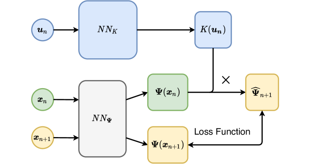
Figure 1: The neural network architecture of PK-NN. The trainable parameters of $K(\bm{u};\bm{\theta}_{K})$ are integrated within the structure of $NN_{K}$, and a distinct neural network $NN_{\bm{\Psi}}$ is used to parametrize the dictionaries $\bm{\Psi}(\bm{x};\bm{\theta}_{\psi})$.

Algorithm 1 Parametric Koopman decomposition with neural networks (PK-NN)

  Data: $\{\bm{x}_{n+1}^{(m)},\bm{x}_{n}^{(m)},\bm{u}_{n}^{(m)}\}_{n,m=0}^{N-1,M-1}$

  Initialize: Random $(\bm{\theta}_{K},\bm{\theta}_{\psi})$.

   Set learning rate $\delta>0$; tolerance $\varepsilon>0$; optimizer Opt.

  while $L(\bm{\theta}_{K},\bm{\theta}_{\psi})>\varepsilon$ do

     Evaluate $L(\bm{\theta}_{K},\bm{\theta}_{\psi})=\sum_{n,m=0}^{N-1,M-1}||\bm{\Psi}(\bm{x}_{n+1}^{(m)};\bm{\theta}_{\psi})-K(\bm{u}_{n}^{(m)};\bm{\theta}_{K})\bm{\Psi}(\bm{x}_{n}^{(m)};\bm{\theta}_{\psi})||^{2}$;

     Update trainable parameters $(\bm{\theta}_{K},\bm{\theta}_{\psi})$ using Opt to minimize $L(\bm{\theta}_{K},\bm{\theta}_{\psi})$;

  end while

We close the presentation of our approach with a discussion on related methodologies. We begin with neural network architectural design. For the dictionary network $\bm{\Psi}$, we essentially follow the approaches in [28, 56] by incorporating $\bm{g}$ into $\bm{\Psi}$ via linear transformations, so that $\bm{g}$ can be recovered by a linear operation (e.g. $\bm{g}=B\bm{\Psi}$). When $\bm{g}$ is high-dimensional, one may alternatively employ non-linear variants and recover $\bm{g}$ from $\bm{\Psi}$ with a trained decoder network [11, 31, 34, 35, 50]. These variants can be readily incorporated into our parametric framework. For the projected Koopman operator network $K$, our method can be viewed as an adaptive version of that introduced in [53], which writes $K(\bm{u})$ as a linear combination $\sum_{i}^{N_{K}}K_{i}h_{i}(\bm{u})$, with $h_{i}$ fixed and $K_{i}$ are fitted from data. If we use a fully connected network to parametrize $K$, then our method generalizes this approach by also training $h_{i}$. More generally, our method allows for alternative architectures for $K$, beyond fixed or adaptive basis expansions.

Let us further contrast our approach with other existing Koopman operator based approaches for non-autonomous systems. The first class of methods posits a linear (or Bilinear) system in the observable space [39, 49, 25, 27], e.g. $\bm{\Psi}_{n+1}=A\bm{\Psi}_{n}+B\bm{u}_{n}$. These have the advantage of linearity, but as we will show in Section 4 that the linearity (or bilinearity) assumption may be too strong for some applications. These can be seen as a special case of our approach with $\mathcal{K}(\bm{u})$ affine in $\bm{u}$. A recent generalization of these methods [10] considers a non-linear transformation of the parameter $\bm{u}$, i.e., systems of the form $\bm{\Psi}_{n+1}=A\bm{\Psi}_{n}+B\mathbf{\Phi}(\bm{u}_{n})$. Another class of methods regard a parametric dynamical system as an autonomous one in the extended state space $X\times U$, which in the most general case, will result in parameter dependent invariant subspaces (i.e. $\bm{\Psi}$ = $\bm{\Psi}(\bm{x},\bm{u})$), unless some further linearity assumptions are introduced [40]. This framework has been applied to control problems [44]. Alternatively, the recent work [20] posits a separable form for the dictionaries $\bm{\Psi}(\bm{x},\bm{u})=G(\bm{u})H(\bm{x})$. If such a form exists, then $H(\bm{x})$ spans a common invariant subspace. In this sense, our method (Proposition 3.1) gives a different approach to construct a common invariant subspace, at least approximately.

3.3 Parametric Koopman analysis for prediction and control

After PK-NN is trained, we can leverage it to solve prediction and control problems in the same family of parametric dynamics.

Prediction problems.

We start with prediction problems. In this scenario, an initial value $\bm{x}_{0}$ and one choice of constant parameter $\bm{u}$ or a sequence of parameters $\{\bm{u}_{n}\}$ are given. The goal is to predict the sequence of observable values $\{\bm{g}(\bm{x}_{n})\}$ generated by the underlying dynamics. Recall that $\bm{g}$ is a given vector valued observable function, which by design is in the span of $\bm{\Psi}$, i.e. $\bm{g}=B\bm{\Psi}$ where $B$ is defined in Eq. 8. The prediction algorithm is summarized in Algorithm 2 for the time-varying parameters case, and the constant parameter case simply replaces all $\bm{u}_{n}$ with $\bm{u}$.

Algorithm 2 Prediction by PK-NN.

  Initial state: $\bm{x}_{0}$. Parameters: $\{\bm{u}_{n}\}_{n=0}^{N-1}$.

  $\widehat{\bm{\Psi}}_{0}=\bm{\Psi}\left(\bm{x}_{0}\right)$.

  for $0\leq n\leq N-1$ do

      $\widehat{\bm{\Psi}}_{n+1}=K(\bm{u}_{n})\widehat{\bm{\Psi}}_{n}$;$\hat{\bm{y}}_{n+1}=B\widehat{\bm{\Psi}}_{n+1}$;

  end for

  Output:$\{\hat{\bm{y}}_{n}\}_{n=1}^{N}$.

Optimal control problems.

In the opposite direction, PK-NN enables us to solve a variety of inverse-type problems, where the goal is to perform inference or optimization on the space of parameters $U$, e.g. system identification. In this work, we focus on the particularly challenging class of such problems in the form of optimal control problems. Concretely, we consider the discrete Bolza control problem whose cost function depends on the observable values

(10) $$\begin{split}\min_{\{\bm{u}_{n}\}_{n=0,1,\dots,N-1}}\quad&J\left[\{\bm{u}_{n}\}\right]=\Phi(\bm{g}(\bm{x}_{N}))+\sum_{n=1}^{N}L_{n}(\bm{g}(\bm{x}_{n}),\bm{u}_{n-1})\\ \text{s.t.}\quad&\bm{x}_{n+1}=\bm{f}(\bm{x}_{n},\bm{u}_{n}).\end{split}$$

Here the initial condition, the terminal cost $\Phi$ and the running costs $L_{n}$ are given, but the dynamics $\bm{f}$ is unknown. Note that in the fully observed case ($\bm{g}(\bm{x})=\bm{x}$), this is a standard Bolza problem. After the construction of $\bm{\Psi}$ and $K$ from data, PK-NN transforms Eq. 10 into

(11) $$\begin{split}\min_{\{\bm{u}_{n}\}_{n=0,1,\dots,N-1}}\quad&J\left[\{\bm{u}_{n}\}\right]=\Phi(B\widehat{\bm{\Psi}}_{N})+\sum_{n=1}^{N}L_{n}(B\widehat{\bm{\Psi}}_{n},\bm{u}_{n-1})\\ \text{s.t.}\quad&\widehat{\bm{\Psi}}_{n+1}=K(\bm{u}_{n})\widehat{\bm{\Psi}}_{n},\\ &\widehat{\bm{\Psi}}_{0}=\bm{\Psi}(\bm{x}_{0}),\end{split}$$

which can be solved using standard optimization libraries. A concrete example is the tracking problem [46, 25], with the objective of achieving precise following of a desired reference observable trajectory $\{\bm{r}_{n}\}_{n=0}^{N}$. In this case, $\Phi\equiv 0$ and $L_{n}(\bm{y},\bm{u})=\|\bm{y}-\bm{r}_{n}\|^{2}$.

It is of particular importance to discuss the case where the control problem does not concern the full state $\bm{x}$, but only some pre-defined observables of it. A simple example is a tracking problem that only requires tracking the first coordinate of the state. In this case, the dictionaries $\bm{\Psi}$ are only required to include the map $\bm{g}(\bm{x})=x_{1}$. Thus, one can understand our approach as a Koopman-operator-assisted model reduction method for data-driven control.

In the literature, there exists control approaches which limits to a finite number of control choices, such as those described in [37] and [2]. These transform the dynamic control problem into a set of autonomous representations and time-switching optimization problems. In particular, [2] leverages input-parameterized Koopman eigenfunctions to handle systems with finite control options, embedding the control within the Koopman eigenfunctions to solve the control problems for the system with fixed points. In contrast, PK-NN allows for control values to be chosen arbitrarily within a predefined range, without being restricted to a set of finite, predetermined options. This feature gives our approach greater flexibility in tackling a variety of control problems.

Compared to existing data-driven approaches, there are some distinct advantages of transforming Eq. 10 into Eq. 11. First, compared with methods that learn linear or bilinear control systems in the observable space [39, 49], the transformed problem Eq. 11 is valid for general dynamics, where $\bm{f}$ may be strongly non-linear in both the state and the control. In these cases, we observe more significant improvements using our method (See Section 4.2). Second, we contrast with the alternative approach of first learning $\bm{f}$ in Eq. 10 using existing non-linear system identification techniques [8, 30, 51], and then applying optimal control algorithms directly to Eq. 10. While this approach is feasible for low-dimensional systems, it becomes inefficient when dealing with high-dimensional non-linear systems, where the control objectives only depend on a few low-dimensional observables. Our method can avoid the expensive identification of high-dimensional dynamics and the subsequent even more expensive optimal control problem in high dimensions. Instead, we parsimoniously construct a low-dimensional control system in the form of Eq. 11, on which the reduced control problem can be easily solved (See tracking the mass and momentum of Korteweg-De Vries (KdV) equation in Section 4.2).

3.4 PK-NN and non-linear controllability

We conclude with a discussion on the interesting subject of controllability. For control problems, and in particular tracking problems, it is desirable that the constructed data-driven state dynamics should be controllable, i.e. the initial state can be driven to an arbitrary target state, at least locally. This gives the system flexibility to track a given trajectory. The controllability rank condition in the lifting space of the Koopman operator analysis with linear dependence on the control is addressed in [6]. Nevertheless, such linear models (as we show in Section 4) have limited modelling capabilities in the general non-linear setting, prompting us to consider the controllability of PK-NN type Koopman dynamics. In particular, we demonstrate that the dynamics Eq. 11 has the special property that controllability conditions are readily checked, and may even be algorithmically enforced.

We discuss this in the context where the dynamics $\bm{x}_{n+1}=\bm{f}(\bm{x}_{n},\bm{u}_{n})$ is a discretization of a differential equation $\dot{\bm{x}}=\tilde{\bm{f}}(\bm{x},\bm{u})$. A classical sufficient condition for controllability is a corollary of the Chow-Rashevsky theorem [9, 41]: if the family $\mathcal{F}=\{\tilde{\bm{f}}(\cdot,\bm{u}):\bm{u}\in U\}$ is smooth and symmetric (meaning that $-\bm{f}\in\mathcal{F}$ if $\bm{f}\in\mathcal{F}$), then the system is controllable with piecewise constant control if $\text{dim Lie}_{\bm{x}}\mathcal{F}=d$ for each $\bm{x}$, where $\text{Lie}_{x}\mathcal{F}$ is the span of the Lie algebra generated by $\mathcal{F}$ at $\bm{x}$. While useful, this condition is difficult to check for a given $\tilde{\bm{f}}$, as it requires the generation of Lie algebras at every point in the state space, unless each member of $\mathcal{F}$ is linear. This is the fundamental difficulty to ensure, or even verify the controllability of non-linear systems.

However, it turns out that controllability is much easier to check for the transformed system under parametric Koopman operator analysis. Concretely, we may compute the corresponding projected Koopman operator (generator) for the continuous system as $\tilde{K}(\bm{u})=(K(\bm{u})-I)/\Delta t$ where $I$ is an identity matrix and $\Delta t$ is the time-discretization step size. The continuous analogue to (11) is thus $\dot{\bm{\Psi}}=\tilde{K}(\bm{u})\bm{\Psi}$. Then, the control family $\mathcal{F}=\{\tilde{K}(\bm{u})(\cdot):\bm{u}\in U\}$ is now a family of linear functions. Therefore, the controllability conditions can be checked at one (any) state, and automatically carries over to all states. We note that this notion of controllability is not over the original state space, but over the (approximately) invariant subspace spanned by $\bm{\Psi}$. In this sense, we can understand the parametric Koopman approach as one that constructs an invariant subspace of observables with the property that controllability in this subspace at any point carries over to the whole subspace – a desirable property of linear control systems.

One way to verify controllability is as follows. Let $\text{Lie}_{\bm{x}}^{(0)}\mathcal{F}\triangleq\text{span}\{\tilde{K}(\bm{u})\bm{x}:\bm{u}\in U\}$. We know that $\text{Lie}_{\bm{x}}^{(0)}\mathcal{F}\subseteq\text{Lie}_{\bm{x}}\mathcal{F}$. Then, $\text{dim Lie}_{\bm{x}}\mathcal{F}=d$ can be guaranteed by $\text{dim Lie}_{\bm{x}}^{(0)}\mathcal{F}=d$, which is equivalent to: for any non-zero vectors $\bm{v}_{1},\bm{v}_{2}\in\mathbb{R}^{d}$, there exists $\bm{u}_{j}\in U$ such that $\bm{v}_{1}^{T}\tilde{K}(\bm{u}_{j})\bm{v}_{2}\neq 0$. This can be ensured if the flattened matrices $\{\tilde{K}(\bm{u}):\bm{u}\in U\}$ do not lie in a proper subspace. Algorithmically, we collect a large sample of parameters $\bm{u}_{i}$, $i=1,2,\dots,N$, flatten each matrix $\tilde{K}(\bm{u}_{i})\in\mathbb{R}^{d\times d}$ into a vector $\bm{k}_{i}\in\mathbb{R}^{d^{2}}$ and concatenate all $\bm{k}_{i}^{{}^{\prime}}$s as a $d^{2}\times N$ matrix

(12) $$C=[\bm{k}_{1},\bm{k}_{2}\dots,\bm{k}_{N}].$$

If the rank of $C=d^{2}$, then the system is controllable. We show in Section 4.2 that this can be readily checked for a learned PK-NN system, and moreover, that it may guide architecture designs for $\bm{u}\mapsto K(\bm{u})$ that promote controllability, yielding an approach that finds a parsimonious controllable dynamics in the observable space. This is an interesting future research direction.

4 Numerical experiments

In this section, we present numerical results on a variety of prediction and control problems. We evaluate various baseline methods, noting that some of these overlap in different aspects of the comparison. For convenience, we introduce a standard format to refer to these methods in Table 1. The code to reproduce these experiments are found at [17].

Table 1: Summary of comparisons. “NN” stand for (residual) neural networks and “RBF” refers to dictionaries built from random radial basis functions. $u_{n,i}$ is the $i^{\text{th}}$ component of $\bm{u}_{n}$.

	Method Description	$\bm{\Psi}$	Reference	Notation
	$\bm{\Psi}(\bm{x}_{n+1})=K\bm{\Psi}(\bm{x}_{n})$	NN	[28]	M1
	$\bm{\Psi}(\bm{x}_{n+1})=A\bm{\Psi}(\bm{x}_{n})+B\bm{u}_{n}$	NN	[39]	M2
	$\bm{\Psi}(\bm{x}_{n+1})=A\bm{\Psi}(\bm{x}_{n})+\sum_{i}B_{i}u_{n,i}\bm{\Psi}(\bm{x}_{n})$	NN	[49]	M3
	$\bm{\Psi}(\bm{x}_{n+1})=\sum_{i=1}^{M}h_{i}(\bm{u}_{n})K_{i}\bm{\Psi}(\bm{x}_{n})$	RBF	[53]	M4-RBF
	$M$ is fixed and $h_{i}$ are fixed polynomials	NN		M4-NN
	$\bm{\Psi}(\bm{x}_{n+1})=K(\bm{u}_{n})\bm{\Psi}(\bm{x}_{n})$	NN		Ours

We first demonstrate on prediction problems that PK-NN outperforms existing methods, including EDMD with dictionary learning (M1) in Section 4.1.1, linear (M2) and bilinear (M3) extensions to systems with parameters or control in Section 4.1.2 and a modified form of EDMD (M4) in Section 4.1.3. In the reverse direction, we show that PK-NN can solve data-driven optimal control problems in Section 4.2. Notably, our approach exhibits more significant improvements for problems with strong non-linearity, or those involving high-dimensional states and parameters.

4.1 Prediction problems

Using Algorithm 2, we test the performance of PK-NN on various forward prediction problems involving discretized parametric ordinary and partial differential equations. Here, the discrete time step $n$ corresponds to the physical time $t_{n}$ of the continuous dynamics, and are equally-spaced. We evaluate performance by the relative reconstruction error at $t_{n}$ on the $m^{\text{th}}$ trajectory is defined as

(13) $$E^{(m)}\left(t_{n}\right)=\frac{\sqrt{\sum_{i=1}^{n}\left\|\hat{\bm{y}}_{i}^{(m)}-\bm{y}_{i}^{(m)}\right\|^{2}}}{\sqrt{\sum_{i=1}^{n}\left\|\bm{y}_{i}^{(m)}\right\|^{2}}},$$

where $\bm{y}_{i}^{(m)}$ is the true value of observables and $\hat{\bm{y}}_{i}^{(m)}$ is the predicted observables at $t_{i}$ on the $m^{\text{th}}$ trajectory. To evaluate the performance on $M$ trajectories, we use the average $E(t_{n})=\frac{1}{M}\sum_{m=1}^{M}E^{(m)}\left(t_{n}\right)$. If there is no special emphasis on the observation function, we set $\bm{g}(\bm{x})=\bm{x}$, the full-state observable.

4.1.1 Improved accuracy and generalization over parameter independent Koopman dynamics

We first demonstrate that PK-NN can interpolate successfully in parameter space and improve upon naively training a separate (parameter-independent) Koopman dynamics for each observed $\bm{u}$ using the method M1 introduced in [28]. We consider the parametric Duffing equation

(14) $$\begin{split}\dot{x_{1}}&=x_{2},\\ \dot{x_{2}}&=-\delta x_{2}-x_{1}\left(\beta+\alpha x_{1}^{2}\right).\end{split}$$

To quantify performance, we use $\nu_{1}$ to denote the number of trajectories for each set of fixed parameters $\bm{u}=(\delta,\alpha,\beta)$ and $\nu_{2}$ to denote the number of different parameter configurations in the dataset. The baseline method trains $\nu_{2}$ separate Koopman dynamics, and at test time chooses one such dynamics with parameter value being the nearest neighbour of the testing parameter. On the other hand, PK-NN trains only one parametric Koopman dynamics that can interpolate over the space of the parameters $\bm{u}$ and directly uses Algorithm 2 to predict. For each configuration of $\nu_{1}$ and $\nu_{2}$, training data is generated with trajectories initialized within the domain $[-2,2]\times[-2,2]$. The parameters $\delta$, $\alpha$ and $\beta$ are randomly sampled from uniform distributions over the intervals $[0,1]$, $[0,2]$ and $[-2,2]$ respectively. To ensure fairness, the total amount of training data $\nu_{1}\times\nu_{2}=10000$ remains constant. For each trajectory, we observe the data points over 50 steps with $\Delta t=0.25$, the same setting as the experiments in [28]. The dictionary $NN_{\psi}$ is constructed as $(1,x_{1},x_{2},NN^{T})^{T}$ where $NN$ is a trainable 22-dimensional vector. This $NN$ is the output of a 3-layer feed-forward ResNet with a width of 100 nodes in each layer. The dictionary by this design is employed in both PK-NN and M1 method. For $NN_{K}$ in PK-NN, we use a 3-layer fully connected neural network with width 256 before the output layer.

Our results, as shown in Fig. 2, indicate that our method more significantly out-performs M1 as $\nu_{2}$ increases. This is because, while we have few representative trajectories per parameter instance (causing M1 to fail), the interpolation in parameter space allows us to integrate information across trajectories with different parameter values, thus ensuring prediction fidelity and generalizability.

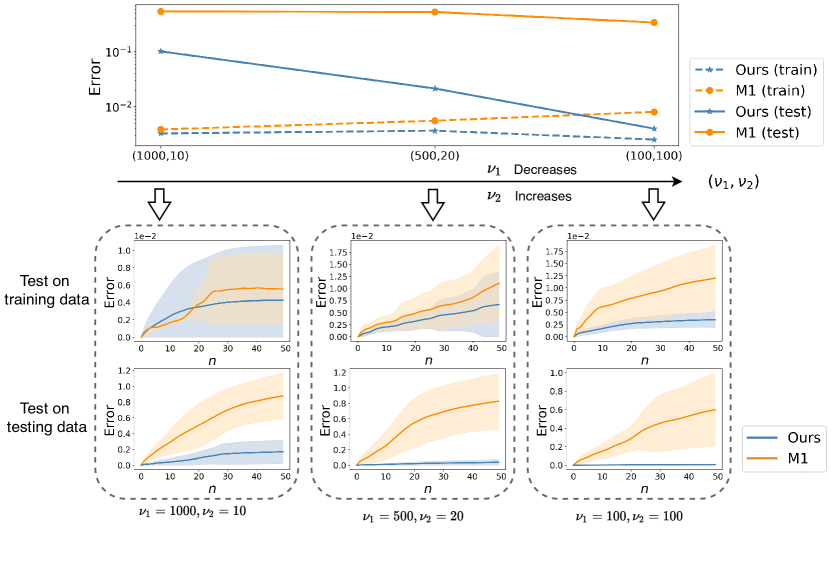
Figure 2: Comparison on different $(\nu_{1},\nu_{2})$ with $\nu_{1}\nu_{2}=10000$. The topmost panel displays the prediction results for PK-NN and M1 on both training and testing data. The horizontal axis represents the values of $(\nu_{1},\nu_{2})$. In the bottom panels, we provide a detailed error analysis at varying time steps across various $(\nu_{1},\nu_{2})$ configurations. We observe that PK-NN out-performs M1 significantly when $\nu_{2}$ increases, which results in fewer trajectories per parameter configuration.

4.1.2 Improved performance on strongly non-linear problems

To see the performance of PK-NN on the problems with strong non-linearity, we test our method on the Van der Pol Mathieu equation [21]

(15) $$\begin{split}\dot{x_{1}}&=x_{2},\\ \dot{x_{2}}&=(k_{1}-k_{2}x_{1}^{2})x_{2}-(w_{0}^{2}+2\mu u^{2}-\mu)x_{1}+uk_{3},\end{split}$$

where $k_{1}=2,k_{2}=2,k_{3}=1$ and $w_{0}=1$. The parameter $u$ is designed to adjust both the parametric excitation $(2\mu u^{2})x_{1}$ and the external excitation $uk_{3}$. The value of the parameter $\mu>0$ captures the non-linearity among $\bm{x}=(x_{1},x_{2})$ and $u$, and this non-linearity becomes more pronounced as the parameter $\mu$ increases. Training data consists of 500 trajectories with $\Delta t=0.01$. Each trajectory spans 50 sampling time steps initialized from a uniformly randomly sampled point in the range of $[-1,1]\times[-1,1]$. The parameter at each time step are also randomly sampled from uniform distributions over $[-1,1]$. In this section, we consider the case where $\nu_{1}=1$ as in Section 4.1.1, thus we do not compare with M1, but instead with the linear Koopman with control approach (M2) [39]

(16) $$\widehat{\bm{\Psi}}_{n+1}=A\widehat{\bm{\Psi}}_{n}+B\bm{u}_{n},$$

and the bilinear variant (M3) [49]

(17) $$\widehat{\bm{\Psi}}_{n+1}=A\widehat{\bm{\Psi}}_{n}+\sum_{i}^{N_{u}}B_{i}u_{n,i}\widehat{\bm{\Psi}}_{n},$$

where $u_{n,i}$’s are the components of vector $\bm{u}_{n}\in\mathbb{R}^{N_{u}}$ and $A,B_{i}$’s $\in\mathbb{R}^{N_{\psi}\times N_{\psi}}$. In experiments, to ensure the effect of dictionaries on state $\bm{x}$ is the same, we use trainable dictionaries which are built by the same network structure and the same dictionary number. The dictionary $NN_{\psi}$ is $(1,x_{1},x_{2},NN^{T})^{T}$ and the dimension of the trainable vector $NN$ is 10. Both $NN$ and $NN_{K}$ employ one hidden layer with width 16. In the experiments, we randomly initialize the dictionary and use the least squares method to get the initial $A$, $B$ or $b_{i}$. To obtain the final results for linear and bilinear models, we train the dictionaries and optimize $A$, $B$ or $b_{i}$ iteratively. For PK-NN, trainable weights are not only contained in dictionaries but also in the projected Koopman operator. We train them together to find an approximately optimal model. As shown in Fig. 3, we show that PK-NN does not perform as well as linear and bilinear model when $\mu=0$ but improves upon them when $\mu=1,2,3,4$. This is expected, since the system is closest to a non-linear/bilinear system when $\mu=0$, whereas it departs more significantly from a linear structure as $\mu$ increases.

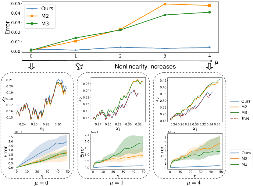
Figure 3: A comparison of errors that occur as the non-linearity of variables $\bm{u}$ and $\bm{x}$ in the problem increases, with the variable $\mu$ acting the non-linearity coefficient. The topmost figure showcases the error analysis for PK-NN, linear model, and bilinear model as the non-linearity coefficient $\mu$ is incremented. The bottom blocks illustrate a contrast between predicted trajectories of different methods and the exact solution, along with an error analysis at each time step for the corresponding $\mu$ configuration. PK-NN outperforms other two structures when the non-linearity of the system increases.

4.1.3 Improved accuracy for high-dimensional systems

We now apply PK-NN to on the high-dimensional problem involving a variation of the FitzHugh-Nagumo partial differential equation subject to quasi-periodic forcing which is mentioned in [53]

(18) $$\begin{split}\partial_{t}v&=\partial_{xx}v+v-v^{3}-w+u(t)(e^{-(x-k_{1})^{2}/2}+e^{-(x-k_{2})^{2}/2}+e^{-(x-k_{3})^{2}/2}),\\ \partial_{t}w&=\delta\partial_{xx}w+\epsilon\left(v-a_{1}w-a_{0}\right).\end{split}$$

where $\delta=4,\epsilon=0.03,a_{1}=2,a_{0}=-0.03,k_{1}=-5,k_{2}=0,k_{3}=5$ on the domain $x\in(-10,10)$ with Neumann boundary conditions. We adopt a finite difference method to discretize the spatial derivatives on a regular mesh consisting of 10 points. In this study, the state vector comprises two components: a 10-dimensional discretized activator complex $\bm{v}$ and a 10-dimensional discretized inhibitor complex $\bm{w}$, resulting in a 20-dimensional state vector. The initial condition for the activator complex $\bm{v}$ is given by $\sin(\frac{a\pi x}{10}+\frac{\pi}{2})$ where $a$ is an integer randomly sampled from the range $(1,20)$. The inhibitor complex $\bm{w}$ is initialized to zero at all spatial points. The parameters $u\in\mathbb{R}$ along the trajectory are uniformly randomly generated in $(-1,1)$. Training data are generated on 100 trajectories over 500 sampling time-steps and $\Delta t=0.001$. We compare PK-NN with the method introduced in [53], which uses fixed radial basis functions as the dictionaries on states and approximates parametric Koopman operator as

(19) $$K(\bm{u})=\sum_{i=1}^{N_{K}}h_{i}(\bm{u})K_{i}.$$

In this experiment, the parameter-dependent functions $h_{i}(\bm{u})$ are approximated by polynomials up to third order. We refer to this method by “M4-RBF” in the following figures. Furthermore, in order to observe the influence of the dictionaries on states, we introduce a modification called “M4-NN”, where the dictionaries are trainable, but the structure of $K(\bm{u})$ is the same as Eq. 19. In this experiment, the dictionary is designed as $(1,\bm{v}^{T},\bm{w}^{T},NN^{T})^{T}$ where $\bm{v},\bm{w}\in\mathbb{R}^{10}$ and $NN$ is 10-dimensional trainable vector. $NN$ utilizes two hidden layers with a width of 128, whereas $NN_{K}$ employs two hidden layers, each with a width of 4.

In Fig. 4(a), we show that trainable dictionaries lead to better prediction results than only using RBF, suggesting that adaptive dictionaries are effective for high-dimensional state spaces. However, we observe that neural network $K(\bm{u})$ performs slightly worse than $K(\bm{u})$ expanded on polynomial basis functions. The reason may be that the dimension of parameter $\bm{u}$ in Eq. 18 is 1, so the approximation of $K(\bm{u})$ may be effectively approximated using polynomials. To verify this hypothesis, we modify Eq. 18 to

(20) $$\begin{split}\partial_{t}v&=\partial_{xx}v+v-v^{3}-w+u_{1}(t)e^{-(x-k_{1})^{2}/2}+u_{2}(t)e^{-(x-k_{2})^{2}/2}+u_{3}(t)e^{-(x-k_{3})^{2}/2},\\ \partial_{t}w&=\delta\partial_{xx}w+\epsilon\left(v-a_{1}w-a_{0}\right).\end{split}$$

with three parameters $\bm{u}=(u_{1},u_{2},u_{3})\in\mathbb{R}^{3}$, while other settings remain unchanged. The number of trainable weights in $K$ are kept approximately the same in both methods, whereas the dimensions of the state dictionary $\bm{\Psi}$ are identical. The dictionary retains a structure of $(1,\bm{v}^{T},\bm{w}^{T},NN^{T})^{T}$. $NN$ utilizes dual hidden layers with a width of 128 and $NN_{K}$ has two hidden layers with width 16. In Fig. 4(b), we observe that PK-NN now performs better than than the two baselines, consistent with our hypothesis.

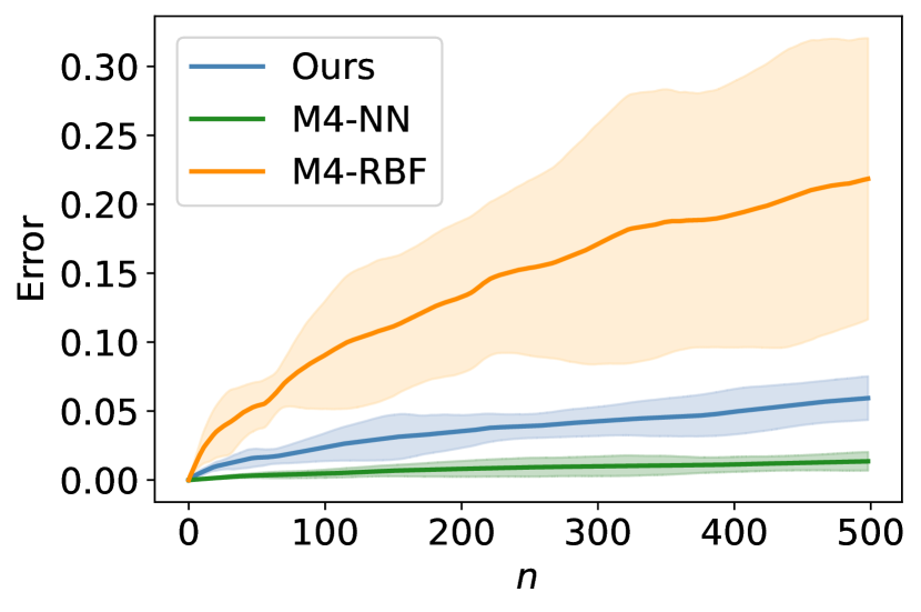
(a) Dim $\bm{u}=1$.

(b) Dim $\bm{u}=3$.

Figure 4: Comparison of prediction errors computed from the three approaches on the FitzHugh-Nagumo PDE discretized on space $\bm{x}$, for varying dimensions of the parameter $\bm{u}$. We observe that as parameter dimension increases, PK-NN out-performs polynomial-based approximation schemes.

4.2 Optimal control problems

As a final class of applications, we show that PK-NN can be used to solve optimal control problems from observational data, without knowledge of the precise form of the dynamics that drive the control system. Furthermore, it can deal with strongly non-linear control systems, both in the state and the control.

We first apply our method to control the forced Korteweg-De Vries (KdV) equation ([32])

(21) $$\frac{\partial\eta(t,x)}{\partial t}+\eta(t,x)\frac{\partial\eta(t,x)}{\partial x}+\frac{\partial^{3}\eta(t,x)}{\partial x^{3}}=w(t,x),$$

where $w(t,x)=\sum_{i=1}^{3}v_{i}(x)\sin(\pi u_{i}(t))$ is the forcing term. Control parameters at $t_{n}$ are $\bm{u}_{n}=(u_{1,n},u_{2,n},u_{3,n})^{T}\in[-1,1]^{3}$. The functions $v_{i}(x)=e^{-25(x-c_{i})^{2}}$ are fixed spatial profiles with $c_{1}=-\frac{\pi}{2}$, $c_{2}=0$ and $c_{3}=\frac{\pi}{2}$ [25]. We consider periodic boundary conditions on the spatial variable $x\in[-\pi,\pi]$ and we discretize with a spatial mesh of 128 points and the time step is $\Delta t=0.01$. This induces a state-space $\bm{\eta}_{n}=(\eta_{1}(t_{n}),\eta_{2}(t_{n}),\dots,\eta_{128}(t_{n}))^{T}$ where $\eta_{i}(t_{n})$ is the value of $\eta(t_{n},x_{i})$ at time $t_{n}$ and $x_{i}$ is the $i^{\text{th}}$ spatial grid point.

We consider a tracking problem involving one of the following two observables: the “mass” $\int_{X}\eta(t,x)dx$ and the “momentum” $\int_{X}\eta^{2}(t,x)dx$. Given a reference trajectory (of either mass or momentum) $\{r_{n}\}$, the tracking problem refers to a Bolza problem (11) with $\Phi\equiv 0$ and $L_{n}(m,\bm{u})=|m-r_{n}|^{2}$. Training data are generated from 1000 trajectories of length 200 samples. The initial conditions are convex combination of three fixed spatial profiles and written as $\eta(0,x)=b_{1}e^{-(x-\frac{\pi}{2})^{2}}+b_{2}(-\sin(\frac{x}{2})^{2})+b_{3}e^{-(x+\frac{\pi}{2})^{2}}$ with $b_{i}>0$ and $\sum_{i=1}^{3}b_{i}=1$, $b_{i}$’s are randomly sampled in $(0,1)$ with uniform distribution. The training controls $u_{i}(t)$ are uniformly randomly generated in $[-1,1]$. We design a common dictionary for the two tracking problems of the form $\bm{\Psi}(\bm{\eta})=(1,\int_{X}\eta(t,x)dx,\int_{X}\eta^{2}(t,x)dx,NN(\bm{\eta}))^{T}$ with 3 trainable elements so that the resulting in the dimension of $\bm{\Psi}$ is 6. The $NN$ is a residual network with two hidden layers having width 16 and $NN_{K}$ has two hidden layers with width 36. The observable matrix $B$ in Eq. 11 is the row vector $(0,1,0,0,0,0)$ for mass tracking, while $B=(0,0,1,0,0,0)$ for momentum tracking.

Instead of computing an optimal control using non-linear programming, we compute $\{\hat{\bm{u}}_{n}\}_{n=0}^{N-1}$ successively in time by solving Eq. 11 with model predictive control (MPC) [16]. We substitute the currently computed control into Eq. 21, which is integrated with RK23 [3] to get the next predicted state $\bm{\eta}_{n+1}$. This map is denoted by $\bm{f}$. The next state is used as the initial value in the next MPC step. In each MPC step, the parametric Koopman dynamics is used to solve for control inputs over a specified time horizon $\tau$ by minimizing the cost function [25]. Concretely, to obtain $\hat{\bm{u}}_{n}$ we solve the optimization problem

(22) $$\begin{split}\min_{\{\tilde{\bm{u}}_{i}\}_{i=n}^{n+\tau-1}}&\quad J=\sum_{i=n}^{n+\tau-1}\left(\|r_{i+1}-m_{i+1}\|^{2}+\lambda\|\tilde{\bm{u}}_{i}\|^{2}\right)\\ \text{s.t.}&\quad m_{i+1}=B\prod_{j=0}^{i-n}K(\tilde{\bm{u}}_{n+j})\bm{\Psi}(\hat{\bm{\eta}}_{n}),\quad i=n,\dots,n+\tau-1,\\ &\quad\hat{\bm{\eta}}_{n}=\bm{f}(\hat{\bm{\eta}}_{n-1},\hat{\bm{u}}_{n-1}),\quad\hat{\bm{\eta}}_{0}=\bm{\eta}_{0},\\ &\quad-1\leq u_{k,n}\leq 1,\quad k=1,2,3,\end{split}$$

giving $\{\tilde{\bm{u}}_{i}\}_{i=n}^{n+\tau-1}$, and then set $\hat{\bm{u}}_{n}=\tilde{\bm{u}}_{n}$. We iterate this for $n=0,1,\dots,N_{T}$ where $N_{T}$ is the number of all time steps in the control problem. Here, $\lambda\geq 0$ is a regularization coefficient.

In experiments, we compare three approaches: PK-NN, M2 (16) and M3 (17). All approaches utilize trainable state dictionaries with identical structures. The starting values of the tracking are computed by the state $\bm{\eta}(t_{0})=0.2$, then we get $m^{(\text{mass})}_{0}=1.27$ and $m^{(\text{momentum})}_{0}=0.25$. Our objective involves tracing the mass or momentum reference trajectories

$$\begin{aligned} r^{(\text{mass})}_{n}=\begin{cases}1.90,&\text{for }n\leq 500\\ 3.16,&\text{for }n>500\end{cases},\quad r^{(\text{momentum})}_{n}=\begin{cases}0.57,&\text{for }n\leq 500\\ 1.58,&\text{for }n>500\end{cases}.\end{aligned}$$

In Fig. 5, we present the tracking results for mass (a) and momentum (b) with the MPC horizon $\tau$ set to 10. When $\lambda=0.005$, PK-NN exhibits better tracking capabilities than the other two methods, attributed to its ability to capture the inherent non-linearity present in Eq. 21. Furthermore, when considering mass tracking under $\lambda=0$, Eq. 21 admits an explicit optimal control solution $u_{i,n}=\frac{1}{2}$ for $0\leq n\leq 59$ and $500\leq n\leq 619$ while $u_{i,n}=0$ otherwise. This follows directly form integrating Eq. 21 over the spatial domain. The evolution of mass under this optimal control is labelled as “KdV” in figure (a) of Fig. 5. In the case of linear and bilinear models, the absence of regularization in optimization leads to failure of mass tracking, due to the fact that the optimal control takes on the values $\pm 1$ i.e. on boundaries of the control set. Over this switching range, the control function $w(t,\cdot)$ cannot be well approximated by a linear function. Similarly, for momentum tracking (Fig. 5(b)), PK-NN outperforms the other two methods, which struggle to track the reference.

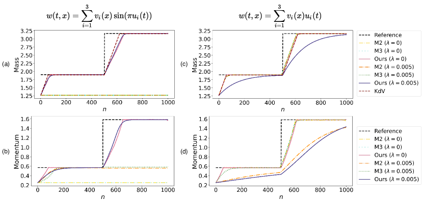
Figure 5: Tracking results for KdV equation utilizing a piece-wise constant reference trajectory. Subfigures (a)-(b) illustrate tracking performance for mass and momentum observables under $w(t,x)=\sum_{i=1}^{3}v_{i}(x)\sin(\pi u_{i}(t))$; Subfigures (c)-(d) present the same tracking comparison when $w(t,x)=\sum_{i=1}^{3}v_{i}(x)u_{i}(t)$.

To confirm that the performance disparity is due to the non-linear dependence of the evolution equations on the control, we perform an ablation study by setting $w(t,x)$ in Eq. 21 to be $\sum_{i=1}^{3}v_{i}(x)u_{i}(t)$, i.e. the forcing term depends linearly on the control. For $\lambda=0$, a similar explicit optimal control can be derived ($u_{i,n}=1$ when $0\leq n\leq 59$ and $500\leq n\leq 619$, and $u_{i,n}=0$ otherwise). As expected, when the control system is linear, the tracking outcomes of these three approaches are similar when $\lambda=0$ and PK-NN is out-performed when $\lambda=0.005$, as depicted in Fig. 5(c) and (d).

We end with an analysis of controllability of the learned parametric Koopman dynamics as discussed in Section 3.4. Recall that a sufficient condition for controllability is for the matrix $C$ (see Eq. 12) to have full rank. When using a deep fully connected network to approximate $K$, we can control the rank of $C$ by setting $N_{K}$, the number of learned features (the width) of the penultimate layer. In this following, we repeat the previous experiments for $N_{K}=37,13,7$. After training, we uniformly randomly sample 2000 $\bm{u}_{i}\in U$ to compute the matrix $C$. The decay of the singular values of $C$ are shown in Fig. 6(a). Note that the dictionary state space is $6$, hence only the case $N_{K}=37$ satisfies the rank condition that guarantees controllability. We now solve the tracking problem under the three choices of $N_{K}$ for $\lambda=0.005$, and the results shown in Fig. 6(b) and Fig. 6(c) confirms that the tracking performance improves with greater controllability. A detailed discussion can be found in Appendix C.

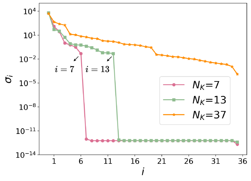
(a) Singular values of $C$.

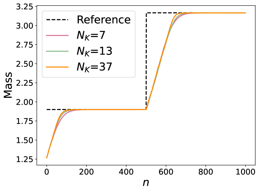
(b) Track mass.

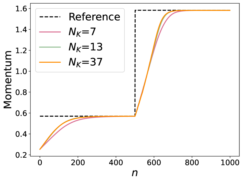
(c) Track momentum.

Figure 6: Comparison on the controllability of PK-NN with $N_{K}=7,13,37$.

5 Conclusion

We propose and implement a data-driven approach for constructing approximate Koopman dynamics for parametric dynamical systems. We utilize neural networks to parametrize both the projected Koopman operator and the state dictionary spanning a common invariant subspace, and simultaneously train them with trajectory data. This allows us to handle high-dimensional and strongly non-linear problems, making it particularly well-suited for applications in large-scale data-driven prediction and control problems.

Appendix A Proof of Proposition 2.1

Proof A.1.

For each $\bm{u}$, we suppose $\mathcal{K}(\bm{u})$ is the composition operator induced by $\bm{f}(\cdot,\bm{u})$. We consider $S\in\mathcal{S}$ such that $m(S)<\infty$, then the indicator function $\mathbf{1}_{S}\in L^{2}(X,m)$. If $\bm{x}\in\bm{f}^{-1}(\cdot,\bm{u})(S)$, we have $\bm{f}(\bm{x},\bm{u})\in S$ since $\bm{f}(\cdot,\bm{u})$ is non-singular. It is equivalent to $(\mathbf{1}_{S}\circ\bm{f}(\cdot,\bm{u}))(\bm{x})=1$, which induces $\mathcal{K}(\bm{u})\mathbf{1}_{S}(\bm{x})=1$. Thus, we have $\mathcal{K}(\bm{u})\mathbf{1}_{S}=\mathbf{1}_{\bm{f}^{-1}(\cdot,\bm{u})(S)}$. Then we have

(23) $$\begin{split}m(\bm{f}^{-1}(\cdot,\bm{u})(S))&=\int\mathbf{1}_{\bm{f}^{-1}(\cdot,\bm{u})(S)}dm\\ &=\int\mathcal{K}(\bm{u})\mathbf{1}_{S}dm\\ &=\int|\mathcal{K}(\bm{u})\mathbf{1}_{S}|^{2}dm\\ &=\|\mathcal{K}(\bm{u})\mathbf{1}_{S}\|^{2}\\ &\leq\|\mathcal{K}(\bm{u})\|^{2}\|\mathbf{1}_{S}\|^{2}\\ &=\|\mathcal{K}(\bm{u})\|^{2}m(S),\end{split}$$

where $\|\mathcal{K}\|=\sup_{\|\phi\|=1}\|\mathcal{K}\phi\|$. Let $b_{\bm{u}}=\|\mathcal{K}(\bm{u})\|^{2}$. Then we have $m(\bm{f}(\cdot,\bm{u})^{-1}(S))\leq b_{\bm{u}}m(S)$.

Conversely, if we have $m(\bm{f}^{-1}(\cdot,\bm{u})(S))\leq b_{\bm{u}}m(S)$, then $m\bm{f}^{-1}(\cdot,\bm{u})\ll m$ (“$\ll$” means absolute continuity). The Radon-Nikodym derivative $h_{\bm{f}(\cdot,\bm{u})}$ of $m\bm{f}^{-1}(\cdot,\bm{u})$ with respect to $m$ exists and $h_{\bm{f}(\cdot,\bm{u})}\leq b_{\bm{u}}$ almost everywhere. Let $\phi\in L^{2}(X,m)$ and then we have

(24) $$\|\mathcal{K}(\bm{u})\phi\|^{2}=\int|\phi\circ\bm{f}(\cdot,\bm{u})|^{2}dm=\int|\phi|^{2}dm\bm{f}^{-1}(\cdot,\bm{u})=\int|\phi|^{2}h_{\bm{f}(\cdot,\bm{u})}dm\leq b_{\bm{u}}\|\phi\|^{2}.$$

This shows that $\mathcal{K}(\bm{u})$ is a bounded (and continuous) operator on $L^{2}(X,m)$.

Appendix B Proof of Proposition 3.1

In this section, we prove Proposition 3.1. The following Lemma B.1 and Lemma B.3 are necessary for our discussion.

Lemma B.1.

If $(e_{i})_{i=1}^{\infty}$ form an orthonormal basis of space $L^{2}(X,m)$. Define $P_{N}g=\operatorname*{argmin}_{\tilde{g}\in\mathrm{span}((e_{i})_{i=1}^{\infty})}\|\tilde{g}-g\|$, then $P_{N}$ converge strongly to the identity operator $I$.

Proof B.2.

Let $\phi=\sum_{i=1}^{\infty}c_{i}e_{i}$ with $\|\phi\|=1$. Then by Parseval’s identity $\sum_{i=1}^{\infty}|c_{i}|^{2}=1$ and

(25) $$\|P_{N}\phi-\phi\|^{2}=\|\sum_{i=N+1}^{\infty}c_{i}e_{i}\|^{2}=\sum_{i=N+1}^{\infty}|c_{i}|^{2}\to 0,\quad\text{as }N\to\infty.$$

Lemma B.3.

Let $X$ be a measurable space with measure $m$. Given an observable function $\phi\in L^{2}(X,m)\cap C_{b}(X,\mathbb{R})$. Assume that $f(\bm{x},\cdot):U\to X$ is continuous for almost all $\bm{x}\in X$. If (3) holds, then $\mathcal{K}(\cdot)\phi:U\to L^{2}(X,m)$ is continuous on $U$ with respect to $L^{2}$ norm, in the sense that $\lim_{\bm{u}_{n}\to\bm{u}}\|\mathcal{K}(\bm{u}_{n})\phi-\mathcal{K}(\bm{u})\phi\|=0$.

Proof B.4.

Since $\bm{f}(\bm{x},\bm{u}_{n})\to\bm{f}(\bm{x},\bm{u})$ as $\bm{u}_{n}\to\bm{u}$ almost everywhere $\bm{x}\in X$ and $\phi(\bm{x})$ is a continuous function, we have

(26) $$\lim_{\bm{u}_{n}\to\bm{u}}|\phi\circ\bm{f}(\bm{x},\bm{u}_{n})-\phi\circ\bm{f}(\bm{x},\bm{u})|^{2}=0$$

almost everywhere on $X$. Since $|\phi(\bm{x})|\leq M$ on $X$ for some $M\in[0,\infty)$, we have $|\phi\circ\bm{f}(\bm{x},\bm{u}_{n})-\phi\circ\bm{f}(\bm{x},\bm{u})|^{2}\leq 4M^{2}$. By the dominated convergence theorem,

(27) $$\begin{split}\lim_{\bm{u}_{n}\to\bm{u}}\|\mathcal{K}(\bm{u}_{n})\phi-\mathcal{K}(\bm{u})\phi\|^{2}&=\lim_{\bm{u}_{n}\to\bm{u}}\int_{X}|\mathcal{K}(\bm{u}_{n})\phi(\bm{x})-\mathcal{K}(\bm{u})\phi(\bm{x})|^{2}m(d\bm{x})\\ &=\lim_{\bm{u}_{n}\to\bm{u}}\int_{X}|\phi\circ\bm{f}(\bm{x},\bm{u}_{n})-\phi\circ\bm{f}(\bm{x},\bm{u})|^{2}m(d\bm{x})\\ &=\int_{X}\lim_{\bm{u}_{n}\to\bm{u}}|\phi\circ\bm{f}(\bm{x},\bm{u}_{n})-\phi\circ\bm{f}(\bm{x},\bm{u})|^{2}m(d\bm{x})\\ &=0.\end{split}$$

Therefore, $\lim_{\bm{u}_{n}\to\bm{u}}\|\mathcal{K}(\bm{u}_{n})\phi-\mathcal{K}(\bm{u})\phi\|=0$.

In Proposition B.5, we demonstrate that an inequality employed in the proof of Proposition 3.1 is applicable to a finite set of parameters for given observables.

Proposition B.5.

Let $U=\{\bm{u}_{1},\bm{u}_{2},\dots,\bm{u}_{s}\}$ be a finite set of parameters and assume that the observables of interest $\bm{g}$ satisfy $g_{j}\in L^{2}(X,m)\cap C_{b}(X)$. Then, for any $\varepsilon>0$, there exists a positive integer $N_{\psi}>0$, a dictionary $\bm{\Psi}=\{\psi_{1},\dots,\psi_{N_{\psi}}\}$ with $\psi_{i}\in L^{2}(X,m)$, a set of vectors $\{\bm{a}_{j}\in\mathbb{R}^{N_{\psi}}:j=1,\dots,N_{y}\}$, such that $g_{j}=\bm{a}_{j}^{T}\bm{\Psi}$ and for all $\bm{u}\in U$, we have $\|\mathcal{K}(\bm{u})g_{j}-P_{N_{\psi}}\mathcal{K}(\bm{u})g_{j}\|\leq\varepsilon$, where $P_{N_{\psi}}g=\operatorname*{argmin}_{\tilde{g}\in\mathrm{span}(\bm{\Psi}_{N_{\psi}})}\|\tilde{g}-g\|$.

Proof B.6.

Let $\psi_{j}=g_{j},j=1,\dots,N_{y}$ and this can ensure the existence of $\bm{a}_{j}$. Let $(\psi_{i})_{i=1}^{\infty}$ be a sequence of functions in $L^{2}$ such that $\mathrm{span}((\psi_{i})_{i=1}^{\infty})$ is dense in $L^{2}$. The dictionary $\bm{\Psi}_{N}=(\psi_{1}(\bm{x}),\psi_{2}(\bm{x}),\dots,\psi_{N}(\bm{x}))^{T}$ consists of the first $N$ elements of $(\psi_{i})_{i=1}^{\infty}$. Then we can compute an orthonormal basis $(e_{i})_{i=1}^{N}$ of $\mathrm{span}(\bm{\Psi}_{N})$ by Gram-Schmidt process and note $(e_{i})_{i=1}^{\infty}$ as an orthonormal basis of $L^{2}$ space. Thus, $\mathrm{span}(\bm{\Psi}_{N})=\mathrm{span}((e_{i})_{i=1}^{N})$ and $P_{N}g=\operatorname*{argmin}_{\tilde{g}\in\mathrm{span}((e_{i})_{i=1}^{N})}\|\tilde{g}-g\|$ by definition.

For each $\bm{u}_{i}\in U$, we have $\bm{x}_{n+1}=\bm{f}(\bm{x}_{n},\bm{u}_{i})$ and $g_{j}(\bm{x}_{n+1})=\mathcal{K}(\bm{u}_{i})g_{j}(\bm{x}_{n})$. By Lemma B.1, for any $\varepsilon_{i}>0$, there exists $N_{i,j}^{*}\in\mathbb{N}^{+}$ such that $N_{i,j}\geq N_{i,j}^{*}$ implies

(28) $$\frac{\|\mathcal{K}(\bm{u}_{i})g_{j}-P_{N_{i,j}}\mathcal{K}(\bm{u}_{i})g_{j}\|}{\|\mathcal{K}(\bm{u}_{i})g_{j}\|}=\|\frac{\mathcal{K}(\bm{u}_{i})g_{j}}{\|\mathcal{K}(\bm{u}_{i})g_{j}\|}-P_{N_{i,j}}\frac{\mathcal{K}(\bm{u}_{i})g_{j}}{\|\mathcal{K}(\bm{u}_{i})g_{j}\|}\|\leq\varepsilon_{i}$$

for each $j$. Let $N_{i}=\max\{N_{i,j}^{*}\}_{j=1,\dots,N_{y}}$. Then we note that

(29) $$\|\mathcal{K}(\bm{u}_{i})g_{j}-P_{N_{i}}\mathcal{K}(\bm{u}_{i})g_{j}\|=\frac{\|\mathcal{K}(\bm{u}_{i})g_{j}-P_{N_{i}}\mathcal{K}(\bm{u}_{i})g_{j}\|}{\|\mathcal{K}(\bm{u}_{i})g_{j}\|}\|\mathcal{K}(\bm{u}_{i})g_{j}\|\leq\varepsilon_{i}\sqrt{b_{\bm{u}_{i}}}\|g_{j}\|.$$

Given $\varepsilon>0$, we set $\varepsilon_{i}=\frac{\varepsilon}{\sqrt{b_{\bm{u}_{i}}}\max\{\|g_{j}\|\}}$ and $b_{\bm{u}_{i}}$ is the coefficient discussed in Proposition 2.1. Then for each $\bm{u}_{i}$, there exists a corresponding $N_{i}$ such that the inequality (29) holds. Define $N_{\psi}=\max{\{N_{1},N_{2},\dots,N_{n}\}}$, then

(30) $$\|\mathcal{K}(\bm{u}_{i})g_{j}-P_{N_{\psi}}\mathcal{K}(\bm{u}_{i})g_{j}\|\leq\varepsilon$$

holds for all $\bm{u}_{i}\in U_{n}$ and all the given $g_{j}$’s.

Now we have the proof of Proposition 3.1.

Proof B.7.

Step 1: By Lemma B.3, the mapping $\mathcal{K}(\cdot):U\to\mathcal{B}(L^{2})$ is continuous on $U$, then for each given observable $g_{j}$, $\mathcal{K}(\cdot)g_{j}:U\to L^{2}$ is uniformly continuous on compact set $U$. We know that for any $\varepsilon^{\prime}>0$, $\exists\delta_{j}>0$ such that $\|\mathcal{K}(\bm{v})g_{j}-\mathcal{K}(\bm{u})g_{j}\|\leq\varepsilon^{\prime}$ for any $\|\bm{v}-\bm{u}\|\leq\delta_{j}$. Let $\delta=\min\{\delta_{j}\}$. We introduce the notion of a localized neighbourhood around each point $\bm{v}_{i}$ in the set $U$. This neighbourhood is formally defined as

(31) $$B_{i}=\{\bm{u}\in U:\|\bm{v}_{i}-\bm{u}\|\leq\delta,\bm{v}_{i}\in U\},$$

where $\delta$ is a predetermined positive radius. Given the collection $\{B_{i}\}$, it suffices to form an open cover for $U$. By the compactness of $U$, we can assert the existence of a finite subcover, denoted as $\{B_{1},B_{2},\dots,B_{n^{*}}\}$, which is sufficient to entirely cover the set $U$.

For each $g_{j}$, we denote $A_{i,j}=\mathcal{K}(B_{i})g_{j}$ as the image of $B_{i}$ by $\mathcal{K}(\cdot)g_{j}$. Then we have $\|\mathcal{K}(\bm{v}_{i})g_{j}-g^{\prime}\|\leq\varepsilon^{\prime}$ for any $g^{\prime}\in A_{i,j}$ and the collection $\{A_{1,j},A_{2,j},\dots,A_{n^{*},j}\}$ can cover $A_{j}=\mathcal{K}(U)g_{j}$. Naturally, for any $\bm{u}\in B_{i}$, we have $\|\bm{v}_{i}-\bm{u}\|\leq\delta$ and

(32) $$\|\mathcal{K}(\bm{v}_{i})g_{j}-\mathcal{K}(\bm{u})g_{j}\|\leq\varepsilon^{\prime}$$

for all given $g_{j}$’s.

Step 2: Let us consider how to get the dimension $N_{\psi}$ of the dictionary $\bm{\Psi}$ by Proposition B.5. For any $\varepsilon^{\prime}>0$, $N_{\psi}$ can be determined by $\{\bm{v}_{i}\}_{i=1}^{n^{*}}$ which are the centers of $\{B_{i}\}_{i=1}^{n^{*}}$, such that

(33) $$\|\mathcal{K}(\bm{v}_{i})g_{j}-P_{N_{\psi}}\mathcal{K}(\bm{v}_{i})g_{j}\|\leq\varepsilon^{\prime}$$

for any $\bm{v}_{i}\in\{\bm{v}_{i}\}_{i=1}^{n^{*}}$ and all given $g_{j}$’s.

Step 3: Follow step 1, for any $\bm{u}\in B_{i}$ and all given $g_{j}$’s, the corresponding $P_{N_{\psi}}$ can give

(34) $$\begin{split}\|P_{N_{\psi}}\mathcal{K}(\bm{v}_{i})g_{j}-P_{N_{\psi}}\mathcal{K}(\bm{u})g_{j}\|&=\|P_{N_{\psi}}(\mathcal{K}(\bm{v}_{i})g_{j}-\mathcal{K}(\bm{u})g_{j})\|\\ &\leq\|P_{N_{\psi}}\|\|\mathcal{K}(\bm{v}_{i})g_{j}-\mathcal{K}(\bm{u})g_{j}\|\\ &\leq\varepsilon^{\prime}\end{split}$$

since $\|P_{N_{\psi}}\|\leq 1$.

Step 4: We consider the analysis for any $\bm{u}\in U$, then $\bm{u}$ must belong to at least one of the neighbourhoods $\{B_{i}\}_{i=1}^{n^{*}}$. If $\bm{u}\in B_{i}$, we consider (33), (32) and (34) and obtain

(35) $$\begin{split}&\|\mathcal{K}(\bm{u})g_{j}-P_{N_{\psi}}\mathcal{K}(\bm{u})g_{j}\|\\ \leq&\|\mathcal{K}(\bm{u})g_{j}-\mathcal{K}(\bm{v}_{i})g_{j}\|+\|\mathcal{K}(\bm{v}_{i})g_{j}-P_{N_{\psi}}\mathcal{K}(\bm{v}_{i})g_{j}\|+\|P_{N_{\psi}}\mathcal{K}(\bm{v}_{i})g_{j}-P_{N_{\psi}}\mathcal{K}(\bm{u})g_{j}\|\\ \leq&\varepsilon,\end{split}$$

when we set $\varepsilon^{\prime}=\frac{\varepsilon}{3}$.

Step 5: Notice that for any $\bm{u}\in U$, there exists a matrix $K(\bm{u})\in\mathbb{R}^{N_{\psi}\times N_{\psi}}$ such that

(36) $$P_{N_{\psi}}\mathcal{K}(\bm{u})g_{j}=\bm{a}_{j}^{T}K(\bm{u})\bm{\Psi},$$

where $\bm{\Psi}$ is defined as discussed in the proof of Proposition B.5. Since $\mathcal{K}(\cdot)g_{j}:U\to L^{2}$ is continuous on $U$, then $\bm{a}_{j}^{T}K(\cdot)\bm{\Psi}:U\to L^{2}$ is continuous on $U$ for $j=1,2,\dots,N_{y}$. Thus, the entries in $K$ are continuous on $U$. Then we note that $K:U\to\mathbb{R}^{N_{\psi}\times N_{\psi}}$ is a continuous function with respect to Frobenius norm and

(37) $$\|\mathcal{K}(\bm{u})g_{j}-\bm{a}_{j}^{T}K(\bm{u})\bm{\Psi}\|=\|\mathcal{K}(\bm{u})g_{j}-P_{N_{\psi}}\mathcal{K}(\bm{u})g_{j}\|\leq\varepsilon.$$

Appendix C Neural network structure of $K(u)$

In this section, we explore the relationship between the number of nodes in the last hidden layer of neural network structure for $K(\bm{u})$ and the rank of matrix $C$. The structure of $K(\bm{u})$ is illustrated in Fig. 7 and the matrix $C$ is discussed in Section 3.3. We explain this relationship by focusing on the KdV case detailed in Section 4.2. In this experiment, $d=N_{\psi}=6$. The output layer in our neural network configuration for $K(\bm{u})$ is a dense layer that includes a bias term. Therefore, if $N_{(\text{last hidden})}$ is the number of nodes in the last hidden layer, $N_{K}$ should be $N_{(\text{last hidden})}+1$. We can regard the flattened matrix $K(\bm{u})$ as the vector obtained prior to the “reshape” operation. Each element in this vector is computed by $N_{K}$ basis functions. Consequently, the rank of matrix $C$ is determined by $\min\{N_{K},d^{2}\}$.

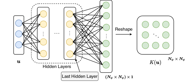
Figure 7: The Neural Networks architecture of $K(\bm{u})$.

References

- [1] H. Arbabi, M. Korda, and I. Mezić, A data-driven koopman model predictive control framework for nonlinear partial differential equations, in 2018 IEEE Conference on Decision and Control (CDC), IEEE, 2018, pp. 6409–6414.
- [2] M. J. Banks, Koopman Representations in Control, PhD thesis, UC Santa Barbara, 2023. ProQuest ID: Banks_ucsb_0035D_16027. Merritt ID: ark:/13030/m5tj9f3g. Retrieved from https://escholarship.org/uc/item/1gg8s7km.
- [3] P. Bogacki and L. F. Shampine, A 3 (2) pair of runge-kutta formulas, Applied Mathematics Letters, 2 (1989), pp. 321–325.
- [4] D. Bruder, X. Fu, R. B. Gillespie, C. D. Remy, and R. Vasudevan, Koopman-based control of a soft continuum manipulator under variable loading conditions, IEEE Robotics and Automation Letters, 6 (2021), pp. 6852–6859.
- [5] D. Bruder, X. Fu, and R. Vasudevan, Advantages of bilinear koopman realizations for the modeling and control of systems with unknown dynamics, IEEE Robotics and Automation Letters, 6 (2021), pp. 4369–4376.
- [6] S. L. Brunton, M. Budišić, E. Kaiser, and J. N. Kutz, Modern koopman theory for dynamical systems, arXiv preprint arXiv:2102.12086, (2021).
- [7] M. Budišić, R. Mohr, and I. Mezić, Applied koopmanism, Chaos: An Interdisciplinary Journal of Nonlinear Science, 22 (2012), p. 047510.
- [8] A. Chiuso and G. Pillonetto, System identification: A machine learning perspective, Annual Review of Control, Robotics, and Autonomous Systems, 2 (2019), pp. 281–304.
- [9] W.-L. Chow, Über systeme von liearren partiellen differentialgleichungen erster ordnung, Mathematische Annalen, 117 (1940), pp. 98–105.
- [10] V. Cibulka, M. Korda, and T. Haniš, Dictionary-free koopman model predictive control with nonlinear input transformation, arXiv preprint arXiv:2212.13828, (2022).
- [11] N. B. Erichson, M. Muehlebach, and M. W. Mahoney, Physics-informed autoencoders for lyapunov-stable fluid flow prediction, arXiv preprint arXiv:1905.10866, (2019).
- [12] C. Folkestad and J. W. Burdick, Koopman nmpc: Koopman-based learning and nonlinear model predictive control of control-affine systems, in 2021 IEEE International Conference on Robotics and Automation (ICRA), IEEE, 2021, pp. 7350–7356.
- [13] C. Folkestad, D. Pastor, I. Mezic, R. Mohr, M. Fonoberova, and J. Burdick, Extended dynamic mode decomposition with learned koopman eigenfunctions for prediction and control, in 2020 american control conference (acc), IEEE, 2020, pp. 3906–3913.
- [14] X. Glorot and Y. Bengio, Understanding the difficulty of training deep feedforward neural networks, in Proceedings of the thirteenth international conference on artificial intelligence and statistics, JMLR Workshop and Conference Proceedings, 2010, pp. 249–256.
- [15] D. Goswami and D. A. Paley, Global bilinearization and controllability of control-affine nonlinear systems: A koopman spectral approach, in 2017 IEEE 56th Annual Conference on Decision and Control (CDC), IEEE, 2017, pp. 6107–6112.
- [16] L. Grüne, J. Pannek, L. Grüne, and J. Pannek, Nonlinear model predictive control, Springer, 2017.
- [17] Y. Guo, M. Korda, I. G. Kevrekidis, and Q. Li, Code repository for learning parametric koopman decompositions, https://github.com/GUOYUE-Cynthia/Learning-Parametric-Koopman-Decompositions.
- [18] D. A. Haggerty, M. J. Banks, P. C. Curtis, I. Mezić, and E. W. Hawkes, Modeling, reduction, and control of a helically actuated inertial soft robotic arm via the koopman operator, arXiv preprint arXiv:2011.07939, (2020).
- [19] M. Haseli and J. Cortés, Temporal forward–backward consistency, not residual error, measures the prediction accuracy of extended dynamic mode decomposition, IEEE Control Systems Letters, 7 (2022), pp. 649–654.
- [20] M. Haseli and J. Cortés, Modeling nonlinear control systems via koopman control family: Universal forms and subspace invariance proximity, arXiv preprint arXiv:2307.15368, (2023).
- [21] H. Jianliang, W. Teng, and C. Shuhui, Nonlinear dynamic analysis of a van der pol-mathieu equation with external excitation, Chinese Journal of Theoretical and Applied Mechanics, 53 (2021), pp. 496–510.
- [22] E. Kaiser, J. N. Kutz, and S. L. Brunton, Data-driven discovery of koopman eigenfunctions for control, arXiv preprint arXiv:1707.01146, (2017).
- [23] D. P. Kingma and J. Ba, Adam: A method for stochastic optimization, arXiv preprint arXiv:1412.6980, (2014).
- [24] B. O. Koopman, Hamiltonian systems and transformation in hilbert space, Proceedings of the national academy of sciences of the united states of america, 17 (1931), p. 315.
- [25] M. Korda and I. Mezić, Linear predictors for nonlinear dynamical systems: Koopman operator meets model predictive control, Automatica, 93 (2018), pp. 149–160.
- [26] M. Korda and I. Mezić, On convergence of extended dynamic mode decomposition to the koopman operator, Journal of Nonlinear Science, 28 (2018), pp. 687–710.
- [27] M. Korda and I. Mezić, Optimal construction of koopman eigenfunctions for prediction and control, IEEE Transactions on Automatic Control, 65 (2020), pp. 5114–5129.
- [28] Q. Li, F. Dietrich, E. M. Bollt, and I. G. Kevrekidis, Extended dynamic mode decomposition with dictionary learning: A data-driven adaptive spectral decomposition of the koopman operator, Chaos: An Interdisciplinary Journal of Nonlinear Science, 27 (2017), p. 103111.
- [29] K. K. Lin and F. Lu, Data-driven model reduction, wiener projections, and the koopman-mori-zwanzig formalism, Journal of Computational Physics, 424 (2021), p. 109864.
- [30] L. Ljung, C. Andersson, K. Tiels, and T. B. Schön, Deep learning and system identification, IFAC-PapersOnLine, 53 (2020), pp. 1175–1181.
- [31] B. Lusch, J. N. Kutz, and S. L. Brunton, Deep learning for universal linear embeddings of nonlinear dynamics, Nature communications, 9 (2018), p. 4950.
- [32] R. M. Miura, The korteweg–devries equation: a survey of results, SIAM review, 18 (1976), pp. 412–459.
- [33] A. Narasingam and J. S.-I. Kwon, Application of koopman operator for model-based control of fracture propagation and proppant transport in hydraulic fracturing operation, Journal of Process Control, 91 (2020), pp. 25–36.
- [34] S. E. Otto and C. W. Rowley, Linearly recurrent autoencoder networks for learning dynamics, SIAM Journal on Applied Dynamical Systems, 18 (2019), pp. 558–593.
- [35] S. Pan and K. Duraisamy, Physics-informed probabilistic learning of linear embeddings of nonlinear dynamics with guaranteed stability, SIAM Journal on Applied Dynamical Systems, 19 (2020), pp. 480–509.
- [36] N. Parmar, H. Refai, and T. Runolfsson, A survey on the methods and results of data-driven koopman analysis in the visualization of dynamical systems, IEEE Transactions on Big Data, (2020).
- [37] S. Peitz and S. Klus, Koopman operator-based model reduction for switched-system control of pdes, Automatica, 106 (2019), pp. 184–191.
- [38] S. Peitz, S. E. Otto, and C. W. Rowley, Data-driven model predictive control using interpolated koopman generators, SIAM Journal on Applied Dynamical Systems, 19 (2020), pp. 2162–2193.
- [39] J. L. Proctor, S. L. Brunton, and J. N. Kutz, Dynamic mode decomposition with control, SIAM Journal on Applied Dynamical Systems, 15 (2016), pp. 142–161.
- [40] J. L. Proctor, S. L. Brunton, and J. N. Kutz, Generalizing koopman theory to allow for inputs and control, SIAM Journal on Applied Dynamical Systems, 17 (2018), pp. 909–930.
- [41] P. Rashevsky, About connecting two points of a completely nonholonomic space by admissible curve, Uch. Zapiski Ped. Inst. Libknechta, 2 (1938), pp. 83–94.
- [42] C. W. Rowley, I. Mezić, S. Bagheri, P. Schlatter, and D. S. Henningson, Spectral analysis of nonlinear flows, Journal of fluid mechanics, 641 (2009), pp. 115–127.
- [43] P. J. Schmid, Dynamic mode decomposition of numerical and experimental data, Journal of fluid mechanics, 656 (2010), pp. 5–28.
- [44] H. Shi and M. Q.-H. Meng, Deep koopman operator with control for nonlinear systems, IEEE Robotics and Automation Letters, 7 (2022), pp. 7700–7707.
- [45] R. K. Singh and J. S. Manhas, Composition operators on function spaces, Elsevier, 1993.
- [46] J.-J. E. Slotine, W. Li, et al., Applied nonlinear control, vol. 199, Prentice hall Englewood Cliffs, NJ, 1991.
- [47] S. H. Son, H.-K. Choi, and J. S.-I. Kwon, Application of offset-free koopman-based model predictive control to a batch pulp digester, AIChE Journal, 67 (2021), p. e17301.
- [48] R. Strässer, J. Berberich, and F. Allgöwer, Robust data-driven control for nonlinear systems using the koopman operator, arXiv preprint arXiv:2304.03519, (2023).
- [49] A. Surana, Koopman operator based observer synthesis for control-affine nonlinear systems, in 2016 IEEE 55th Conference on Decision and Control (CDC), IEEE, 2016, pp. 6492–6499.
- [50] N. Takeishi, Y. Kawahara, and T. Yairi, Learning koopman invariant subspaces for dynamic mode decomposition, Advances in neural information processing systems, 30 (2017).
- [51] D. N. Tanyu, J. Ning, T. Freudenberg, N. Heilenkötter, A. Rademacher, U. Iben, and P. Maass, Deep learning methods for partial differential equations and related parameter identification problems, arXiv preprint arXiv:2212.03130, (2022).
- [52] J. H. Tu, Dynamic mode decomposition: Theory and applications, PhD thesis, Princeton University, 2013.
- [53] M. O. Williams, M. S. Hemati, S. T. Dawson, I. G. Kevrekidis, and C. W. Rowley, Extending data-driven koopman analysis to actuated systems, IFAC-PapersOnLine, 49 (2016), pp. 704–709.
- [54] M. O. Williams, I. G. Kevrekidis, and C. W. Rowley, A data–driven approximation of the koopman operator: Extending dynamic mode decomposition, Journal of Nonlinear Science, 25 (2015), pp. 1307–1346.
- [55] M. O. Williams, C. W. Rowley, and I. G. Kevrekidis, A kernel-based approach to data-driven koopman spectral analysis, arXiv preprint arXiv:1411.2260, (2014).
- [56] E. Yeung, S. Kundu, and N. Hodas, Learning deep neural network representations for koopman operators of nonlinear dynamical systems, in 2019 American Control Conference (ACC), IEEE, 2019, pp. 4832–4839.