Prompt-tuning latent diffusion models
for inverse problems

Abstract

We propose a new method for solving imaging inverse problems using text-to-image latent diffusion models as general priors. Existing methods using latent diffusion models for inverse problems typically rely on simple null text prompts, which can lead to suboptimal performance. To address this limitation, we introduce a method for prompt tuning, which jointly optimizes the text embedding on-the-fly while running the reverse diffusion process. This allows us to generate images that are more faithful to the diffusion prior. In addition, we propose a method to keep the evolution of latent variables within the range space of the encoder, by projection. This helps to reduce image artifacts, a major problem when using latent diffusion models instead of pixel-based diffusion models. Our combined method, called P2L, outperforms both image- and latent-diffusion model-based inverse problem solvers on a variety of tasks, such as super-resolution, deblurring, and inpainting.

1 Introduction

Imaging inverse problems are often solved by optimizing or sampling a functional that combines a data-fidelity/likelihood term with a regularization term or signal prior (Romano et al., 2017; Venkatakrishnan et al., 2013; Ongie et al., 2020; Kamilov et al., 2023; Kawar et al., 2022; Kadkhodaie & Simoncelli, 2021; Chung et al., 2023b). A common regularization strategy is to use pre-trained image priors from generative models, such as GANs  (Bora et al., 2017), VAEs (Bora et al., 2017; González et al., 2022), Normalizing flows (Whang et al., 2021) or Diffusion models (Song et al., 2022; Chung & Ye, 2022).

In particular, diffusion models have gained significant attention as implicit generative priors for solving inverse problems in imaging (Kadkhodaie & Simoncelli, 2021; Whang et al., 2022; Daras et al., 2022; Kawar et al., 2022; Feng et al., 2023; Laroche et al., 2023; Chung et al., 2023b). Leaving the pre-trained diffusion prior intact, one can guide the inference process to perform posterior sampling conditioned on the measurement at inference time by resorting to Bayesian inference. In the end, the ultimate goal of Diffusion model-based Inverse problem Solvers (DIS) would be to act as a fully general inverse problem solver, which can be used not only regardless of the imaging model, but also regardless of the data distribution.

Solving inverse problems in a fully general domain is hard. This directly stems from the difficulty of generative modeling a wide distribution, where it is known that one has to trade-off diversity with fidelity by some means of sharpening the distribution (Brock et al., 2018; Dhariwal & Nichol, 2021). The standard approach in modern diffusion models is to condition on text prompts (Rombach et al., 2022; Saharia et al., 2022b), among them the most popular being Stable Diffusion (SD), a latent diffusion model (LDM), which is itself an under-explored topic in the context of inverse problem solving. While text conditioning is now considered standard practice in content creation including images (Ramesh et al., 2022; Saharia et al., 2022b), 3D (Poole et al., 2023; Wang et al., 2023c), video (Ho et al., 2022), personalization (Gal et al., 2022), and editing (Hertz et al., 2022), it has been completely disregarded in the inverse problem solving context. This is natural, as it is highly ambiguous which text would be beneficial to use when all we have is a degraded measurement. The wrong prompt could easily lead to degraded performance.

In this work, we aim to bridge this gap by proposing a way to automatically find the right prompt to condition diffusion models when solving inverse problems. This can be achieved through optimizing the continuous text embedding on-the-fly while running DIS. We formulate this into a Bayesian framework of updating the text embedding and the latent in an alternating fashion, such that they become gradually aligned during the sampling process. Orthogonal and complementary to embedding optimization, we devise a simple LDM-based DIS (LDIS) that controls the evolution of the latents to stay on the natural data manifold by explicit projection. We name the algorithm that combines these components P2L, short for Prompt-tuning Projected Latent diffusion model-based inverse problem solver. In reaching for the ultimate goal of DIS, we focus on 1) LDM-based DIS (LDIS) for solving inverse problems in the 2) fully general domain (using a single pre-trained checkpoint) that targets 3) 512$\times$512 resolution. All the aforementioned components are highly challenging, and to the best of our knowledge, have not been studied in conjunction before.

	FFHQ						ImageNet
	SR$\times 8$			Inpaint ($p=0.8$)			SR$\times 8$			Inpaint ($p=0.8$)
Prompt	FID$\downarrow$	LPIPS$\downarrow$	PSNR$\uparrow$	FID$\downarrow$	LPIPS$\downarrow$	PSNR$\uparrow$	FID$\downarrow$	LPIPS$\downarrow$	PSNR$\uparrow$	FID$\downarrow$	LPIPS$\downarrow$	PSNR$\uparrow$
""	61.16	0.327	26.49	52.34	0.241	29.78	78.68	0.397	23.49	70.87	0.350	26.20
"A high quality photo"	61.17	0.327	26.57	52.82	0.237	29.70	77.00	0.396	23.51	69.10	0.350	26.26
"A high quality photo of a cat"	69.03	0.377	26.39	55.15	0.248	29.63	76.69	0.402	23.63	68.48	0.355	26.13
"A high quality photo of a dog"	66.55	0.371	26.48	55.91	0.249	29.65	76.45	0.394	23.58	67.75	0.354	26.10
"A high quality photo of a face"	60.41	0.325	26.74	52.33	0.239	29.69	77.32	0.403	23.60	68.83	0.352	26.20
Proposed	58.73	0.317	26.68	51.40	0.233	29.69	66.96	0.386	23.57	66.82	0.314	26.29
PALI prompts from ${\boldsymbol{y}}$	61.33	0.329	26.81	54.34	0.249	29.76	68.28	0.388	23.57	69.55	0.355	26.26
PALI prompts from ${\boldsymbol{x}}$	60.73	0.322	26.76	52.06	0.238	29.75	66.55	0.387	23.57	64.00	0.348	26.17

Table 1: Difference in restoration performance using LDPS on SR$\times 8$ task with varying text prompts. Proposed: text embedding optimized without access to ground truth. PALI prompts from ${\boldsymbol{x}}$/${\boldsymbol{y}}$: captions are generated with PALI (Chen et al., 2022) from ${\boldsymbol{x}}$: ground truth clean images / ${\boldsymbol{y}}$: degraded images. The former can be considered an empirical upper bound.

2 Background

2.1 Latent diffusion models

Diffusion models are generative models that learn to reverse the forward noising process (Sohl-Dickstein et al., 2015; Ho et al., 2020; Song et al., 2021), starting from the initial distribution $p_{0}({\boldsymbol{x}}),\,{\boldsymbol{x}}\in{\mathbb{R}}^{n}$ and approaching the standard Gaussian $p_{T}({\boldsymbol{x}})={\mathcal{N}}(\bm{0},{\bm{I}})$ as $T\rightarrow\infty$. Considering the variance-preserving (VP) formulation (Ho et al., 2020), the forward/reverse processes can be characterized with Ito stochastic differential equations (SDE) (Song et al., 2021)

$$d{\boldsymbol{x}}_{t} =-\frac{\beta_{t}}{2}{\boldsymbol{x}}_{t}dt+\sqrt{\beta_{t}}d{\boldsymbol{w}}$$ (Forward) (1)

$$d{\boldsymbol{x}}_{t} =\left[-\frac{\beta_{t}}{2}{\boldsymbol{x}}-\beta_{t}\nabla_{{\boldsymbol{x}}_{t}}\log p_{t}({{\boldsymbol{x}}_{t}})\right]dt+\sqrt{\beta_{t}}d\bar{\boldsymbol{w}} \text{(Reverse)},$$ (2)

where $\beta_{t}$ is the noise schedule and ${\boldsymbol{w}},\bar{\boldsymbol{w}}$ are the standard forward/reverse Wiener processes. Here $\nabla_{{\boldsymbol{x}}_{t}}\log p_{t}({\boldsymbol{x}}_{t})$ is typically approximated with a score network ${\boldsymbol{s}}_{\boldsymbol{\theta}}(\cdot)$ or a noise estimation network ${\boldsymbol{\epsilon}}_{\boldsymbol{\theta}}(\cdot)$, and learned through denoising score matching (DSM) (Vincent, 2011) or epsilon-matching loss (Ho et al., 2020).

Image diffusion models that operate on the pixel space ${\boldsymbol{x}}$ are compute-heavy. One workaround for compute-efficient generative modeling is to leverage an autoencoder (Rombach et al., 2022; Kingma & Welling, 2013)

$${\mathcal{E}}:{\mathbb{R}}^{n}\mapsto{\mathbb{R}}^{k},\,{\mathcal{D}}:{\mathbb{R}}^{k}\mapsto{\mathbb{R}}^{n},\,{\boldsymbol{x}}\simeq{\mathcal{D}}({\mathcal{E}}({\boldsymbol{x}}))\quad\forall{\boldsymbol{x}}\sim p_{\rm data}({\boldsymbol{x}}),$$ (3)

where ${\mathcal{E}}$ is the encoder, ${\mathcal{D}}$ is the decoder, and $k<n$. After encoding the images into the latent space ${\boldsymbol{z}}={\mathcal{E}}({\boldsymbol{x}})$ (Rombach et al., 2022), one can train a diffusion model in the low-dimensional latent space. Latent diffusion models (LDM) are beneficial in that the computation is cheaper as it operates in a lower-dimensional space, consequently being more suitable for modeling higher dimensional data (e.g. large images of size $\geq 512^{2}$). The effectiveness of LDMs have democratized the use of diffusion models as the de facto standard of generative models especially for images under the name of Stable Diffusion (SD), which we focus on extensively in this work.

One notable difference of SD from standard image diffusion models (Dhariwal & Nichol, 2021) is the use of text conditioning ${\boldsymbol{\epsilon}}_{\boldsymbol{\theta}}(\cdot,{\mathcal{C}})$, where ${\mathcal{C}}$ is the continuous embedding vector usually obtained through the CLIP text embedder (Radford et al., 2021). As the model is trained with LAION-5B (Schuhmann et al., 2022), a large-scale dataset containing image-text pairs, SD can be conditioned during the inference time to generate images that are aligned with the given text prompt by directly using ${\boldsymbol{\epsilon}}_{\boldsymbol{\theta}}(\cdot,{\mathcal{C}})$, or by means of classifier-free guidance (CFG) (Ho & Salimans, 2021).

2.2 Solving inverse problem with (latent) diffusion models

Given access to some measurement

$${\boldsymbol{y}}={\boldsymbol{A}}{\boldsymbol{x}}+{\boldsymbol{n}},\quad{\boldsymbol{x}}\in{\mathbb{R}}^{n},\,{\boldsymbol{y}}\in{\mathbb{R}}^{m},\,{\boldsymbol{A}}\in{\mathbb{R}}^{m\times n},\,{\boldsymbol{n}}\sim{\mathcal{N}}(\bm{0},\sigma_{y}^{2}{\bm{I}}_{m})$$ (4)

where ${\boldsymbol{A}}$ is the forward operator and ${\boldsymbol{n}}$ is additive white Gaussian noise, the task is retrieving ${\boldsymbol{x}}$ from ${\boldsymbol{y}}$. As the problem is ill-posed, a natural way to solve it is to perform posterior sampling ${\boldsymbol{x}}\sim p({\boldsymbol{x}}|{\boldsymbol{y}})$ by defining a suitable prior $p({\boldsymbol{x}})$. In DIS, diffusion models (i.e. denoisers) act as the implicit prior with the use of the score function.

Earlier methods utilized an alternating projection approach, where hard measurement constraints are applied in-between the denoising steps whether in pixel space (Kadkhodaie & Simoncelli, 2021; Song et al., 2021) or measurement space (Song et al., 2022; Chung & Ye, 2022). Distinctively, projection in the spectral space via singular value decomposition (SVD) to incorporate measurement noise has been developed (Kawar et al., 2021; 2022). Subsequently, methods that aim to approximate the gradient of the log posterior in the diffusion model context have been proposed (Chung et al., 2023b; Song et al., 2023b), expanding the applicability to nonlinear problems. Broadening the range even further, methods that aim to solve blind (Chung et al., 2023a; Murata et al., 2023), 3D (Chung et al., 2023d; Lee et al., 2023), and unlimited resolution problems (Wang et al., 2023b) were introduced. More recently, methods leveraging diffusion score functions within variational inference to solve inverse imaging has been proposed (Mardani et al., 2023; Feng et al., 2023). Notably, all the aforementioned methods utilize image-domain diffusion models. Orthogonal to this direction, some of the recent works have shifted their attention to using latent diffusion models (Rout et al., 2023; Song et al., 2023a; He et al., 2023), a direction that we follow in this work.

One canonical DIS that covers the widest range of non-blind problems is diffusion posterior sampling (DPS) (Chung et al., 2023b), which proposes to approximate

$$\nabla_{{\boldsymbol{x}}_{t}}\log p({\boldsymbol{y}}|{\boldsymbol{x}}_{t})\simeq\nabla_{{\boldsymbol{x}}_{t}}\log p({\boldsymbol{y}}|{\mathbb{E}}[{\boldsymbol{x}}_{0}|{\boldsymbol{x}}_{t}]),\quad{\mathbb{E}}[{\boldsymbol{x}}_{0}|{\boldsymbol{x}}_{t}]=\frac{1}{\sqrt{\bar{\alpha}_{t}}}\left({\boldsymbol{x}}_{t}-\sqrt{1-\bar{\alpha}_{t}}{\boldsymbol{\epsilon}}_{{\boldsymbol{\theta}}^{*}}({\boldsymbol{x}}_{t})\right),$$ (5)

where the posterior mean is the result of Tweedie’s formula (Robbins, 1956; Efron, 2011; Chung et al., 2023b). This idea was recently extended to LDMs in a few recent works (Rout et al., 2023; He et al., 2023)

$$\nabla_{{\boldsymbol{z}}_{t}}\log p({\boldsymbol{y}}|{\boldsymbol{z}}_{t})\simeq\nabla_{{\boldsymbol{z}}_{t}}\log p({\boldsymbol{y}}|{\mathcal{D}}({\mathbb{E}}[{\boldsymbol{z}}_{0}|{\boldsymbol{z}}_{t}]))=\nabla_{{\boldsymbol{z}}_{t}}\|{\boldsymbol{y}}-{\mathcal{D}}(\hat{\boldsymbol{z}}_{0})\|_{2}^{2},$$ (6)

with $\hat{\boldsymbol{z}}_{0}:={\mathbb{E}}[{\boldsymbol{z}}_{0}|{\boldsymbol{z}}_{t}]$. We refer to the sampler that uses the approximation in Eq. (6) as Latent DPS (LDPS) henceforth. rout2023solving extends LDPS with an additional regularization term to guide the latent to be the fixed point of the autoencoding process, and he2023iterative extends LDPS by using history updates as in Adam (kingma2015adam). However, all of the existing works in the literature that aims for LDIS, to the best of our knowledge, neglects the use of text embedding by resorting to the use of null text embedding ${\mathcal{C}}_{\varnothing}$.

2.3 Prompt tuning

In modern language models and vision-langauge models, prompting is a standard technique (radford2021learning; brown2020language) to guide the large pre-trained models to solve downstream tasks. As it has been found that even slight variations in the prompting technique can lead to vastly different outcomes (kojima2022large), prompt tuning (learning) has been introduced (shin2020autoprompt; zhou2022learning), which defines a learnable context vector to optimize over. It was shown that by only optimizing over the continuous embedding vector while maintaining the model parameters fixed, one can achieve a significant performance gain.

In the context of diffusion models, prompt tuning has been adopted for personalization (gal2022image), where one defines a special token to embed a specific concept with only a few images. Moreover, it has also been demonstrated that one can achieve superior editing performance by optimizing for the null text prompt ${\mathcal{C}}_{\varnothing}$ (mokady2023null) before the reverse diffusion sampling process.

3 Main Contribution: the P2L algorithm

Algorithm 1 Update ${\mathcal{C}}_{t}$

1:function OptimizeEmb(${\boldsymbol{z}}_{t},{\boldsymbol{y}},{\mathcal{C}}_{t}^{(0)}$)

2:     for $k=1$ to $K$ do

3:         $\hat{\boldsymbol{\epsilon}}_{t}\leftarrow{\boldsymbol{\epsilon}}_{{\boldsymbol{\theta}}^{*}}({\boldsymbol{z}}_{t},{\mathcal{C}}_{t}^{(k-1)})$

4:         $\hat{\boldsymbol{z}}_{0|t}\leftarrow({\boldsymbol{z}}_{t}-\sqrt{1-\bar{\alpha}_{t}}\hat{{\boldsymbol{\epsilon}}}_{t}){/\sqrt{\bar{\alpha}_{t}}}$

5:         $\hat{\boldsymbol{x}}_{0|t}\leftarrow{\mathcal{D}}(\hat{\boldsymbol{z}}_{0|t})$

6:         ${\mathcal{L}}\leftarrow\|{\boldsymbol{A}}\hat{\boldsymbol{x}}_{0|t}({\mathcal{C}}_{t}^{(k-1)})-{\boldsymbol{y}}\|_{2}^{2}$

7:         ${\mathcal{C}}_{t}^{(k)}\leftarrow{\mathcal{C}}_{t}^{(k-1)}-\texttt{AdamGrad}({\mathcal{L}}_{t})$

8:     end for

9:     return ${\mathcal{C}}_{t}^{*}\leftarrow{\mathcal{C}}_{t}^{(K)}$

10:end function

Algorithm 2 Update ${\boldsymbol{z}}_{t}$

1:${\boldsymbol{\epsilon}}_{{\boldsymbol{\theta}}^{*}},{\boldsymbol{z}}_{T},{\boldsymbol{y}},{\mathcal{C}},T,K$

2:for $t=T$ to $1$ do

3:     ${\mathcal{C}}_{t}^{*}\leftarrow\color[rgb]{0,0,0}{\textsc{OptimizeEmb}}({\boldsymbol{z}}_{t},{\boldsymbol{y}},{\mathcal{C}}_{t}^{0})$

4:     $\hat{\boldsymbol{\epsilon}}_{t}\leftarrow{\boldsymbol{\epsilon}}_{{\boldsymbol{\theta}}^{*}}({\boldsymbol{z}}_{t},{\mathcal{C}}_{t}^{*})$

5:     $\hat{\boldsymbol{z}}_{0|t}\leftarrow({\boldsymbol{z}}_{t}-\sqrt{1-\bar{\alpha}_{t}}\hat{{\boldsymbol{\epsilon}}}_{t}){/\sqrt{\bar{\alpha}_{t}}}$

6:     $\color[rgb]{0,0,0}{\hat{\boldsymbol{z}}^{\prime}_{0|t}\leftarrow{\mathcal{E}}\left({\bm{\Gamma}}\left({\mathcal{D}}(\hat{\boldsymbol{z}}_{0|t})\right)\right)}$

7:     ${\boldsymbol{z}}^{\prime}_{t-1}\leftarrow\sqrt{\bar{\alpha}_{t-1}}\hat{\boldsymbol{z}}_{0|t}+\sqrt{1-\bar{\alpha}_{t-1}}\hat{\boldsymbol{\epsilon}}_{t}$

8:     ${\boldsymbol{z}}_{t-1}\leftarrow{\boldsymbol{z}}^{\prime}_{t-1}-\rho_{t}\nabla_{{\boldsymbol{z}}_{t}}\|{\mathcal{A}}{\mathcal{D}}(\hat{\boldsymbol{z}}_{0|t})-{\boldsymbol{y}}\|$

9:     ${\mathcal{C}}_{t-1}^{(0)}\leftarrow{\mathcal{C}}_{t}^{*}$

10:end for

11:return ${\boldsymbol{x}}_{0}\leftarrow{\mathcal{D}}({\boldsymbol{z}}_{0})$

Algorithm 3 Prompt tuning

1:function OptimizeEmb(${\boldsymbol{z}}_{t},{\boldsymbol{y}},{\mathcal{C}}_{t}^{(0)}$)

2:     for $k=1$ to $K$ do

3:         $\hat{\boldsymbol{\epsilon}}_{t}\leftarrow{\boldsymbol{\epsilon}}_{{\boldsymbol{\theta}}^{*}}({\boldsymbol{z}}_{t},{\mathcal{C}}_{t}^{(k-1)})$

4:         $\hat{\boldsymbol{z}}_{0|t}\leftarrow({\boldsymbol{z}}_{t}-\sqrt{1-\bar{\alpha}_{t}}\hat{{\boldsymbol{\epsilon}}}_{t}){/\sqrt{\bar{\alpha}_{t}}}$

5:         $\hat{\boldsymbol{z}}^{\prime}_{0|t}\leftarrow\hat{\boldsymbol{z}}_{0|t}-\rho\nabla_{\hat{\boldsymbol{z}}_{0|t}}\|{\boldsymbol{y}}-{\mathcal{D}}(\hat{\boldsymbol{z}}_{0|t})\|$

6:         $\hat{\boldsymbol{x}}_{0|t}\leftarrow{\mathcal{D}}(\hat{\boldsymbol{z}}^{\prime}_{0|t})$

7:         ${\mathcal{L}}\leftarrow\|{\boldsymbol{A}}\hat{\boldsymbol{x}}_{0|t}({\mathcal{C}}_{t}^{(k-1)})-{\boldsymbol{y}}\|_{2}^{2}$

8:         ${\mathcal{C}}_{t}^{(k)}\leftarrow{\mathcal{C}}_{t}^{(k-1)}-\texttt{AdamGrad}({\mathcal{L}}_{t})$

9:     end for

10:     return ${\mathcal{C}}_{t}^{*}\leftarrow{\mathcal{C}}_{t}^{(K)}$

11:end function

Algorithm 4 P2L

1:${\boldsymbol{\epsilon}}_{{\boldsymbol{\theta}}^{*}},{\boldsymbol{z}}_{T},{\boldsymbol{y}},{\mathcal{C}},T,K,\gamma,\bm{\Gamma}$

2:for $t=T$ to $1$ do

3:     ${\mathcal{C}}_{t}^{*}\leftarrow\color[rgb]{0,0,0}{\textsc{OptimizeEmb}}({\boldsymbol{z}}_{t},{\boldsymbol{y}},{\mathcal{C}}_{t}^{0})$

4:     $\hat{\boldsymbol{\epsilon}}_{t}\leftarrow{\boldsymbol{\epsilon}}_{{\boldsymbol{\theta}}^{*}}({\boldsymbol{z}}_{t},{\mathcal{C}}_{t}^{*})$

5:     $\hat{\boldsymbol{z}}_{0|t}\leftarrow({\boldsymbol{z}}_{t}-\sqrt{1-\bar{\alpha}_{t}}\hat{{\boldsymbol{\epsilon}}}_{t}){/\sqrt{\bar{\alpha}_{t}}}$

6:     if $(t\mod\gamma)=0$ then

7:         $\color[rgb]{0,0,0}{\hat{\boldsymbol{z}}^{\prime}_{0|t}\leftarrow{\mathcal{E}}\left({\bm{\Gamma}}\left({\mathcal{D}}(\hat{\boldsymbol{z}}_{0|t})\right)\right)}$

8:     end if

9:     ${\boldsymbol{z}}^{\prime}_{t-1}\leftarrow\sqrt{\bar{\alpha}_{t-1}}\hat{\boldsymbol{z}}^{\prime}_{0|t}+\sqrt{1-\bar{\alpha}_{t-1}}\hat{\boldsymbol{\epsilon}}_{t}$

10:     ${\boldsymbol{z}}_{t-1}\leftarrow{\boldsymbol{z}}^{\prime}_{t-1}-\rho_{t}\nabla_{{\boldsymbol{z}}_{t}}\|{\mathcal{A}}{\mathcal{D}}(\hat{\boldsymbol{z}}_{0|t})-{\boldsymbol{y}}\|$

11:     ${\mathcal{C}}_{t-1}^{(0)}\leftarrow{\mathcal{C}}_{t}^{*}$

12:end for

13:return ${\boldsymbol{x}}_{0}\leftarrow{\mathcal{D}}({\boldsymbol{z}}_{0})$

3.1 Prompt tuning inverse problem solver

The objective of solving inverse problems is to provide a restoration that is as close as possible to the ground truth given the measurement, whether we are targeting to minimize the distortion or to maximize the perceptual quality (blau2018perception; delbracio2023inversion). Formally, let us denote a loss function ${\mathcal{L}}({\boldsymbol{x}},{\boldsymbol{c}})$ that measures the discrepancy from the ground-truth given the estimate of the truth ${\boldsymbol{x}}$, and some additional condition ${\boldsymbol{c}}$. In the context of LDIS, we consider

$$\operatorname*{arg\,min}_{{\boldsymbol{x}},{\boldsymbol{c}}}{\mathcal{L}}({\boldsymbol{x}},{\boldsymbol{c}})\equiv\operatorname*{arg\,min}_{{\boldsymbol{z}},{\boldsymbol{c}}}{\mathcal{L}}({\mathcal{D}}({\boldsymbol{z}}),{\boldsymbol{c}}),\quad{\boldsymbol{x}}={\mathcal{D}}({\boldsymbol{z}}),$$ (7)

where ${\boldsymbol{c}}$ is the text embedding, ${\mathcal{D}}$ is the decoder of the VAE, and the loss ${\mathcal{L}}$ can be considered as the negative log posterior in the Bayesian framework. It is easy to see that

$$\operatorname*{arg\,min}_{{\boldsymbol{z}},{\boldsymbol{c}}}{\mathcal{L}}({\mathcal{D}}({\boldsymbol{z}}),{\boldsymbol{c}})\leq\operatorname*{arg\,min}_{{\boldsymbol{z}}}{\mathcal{L}}({\mathcal{D}}({\boldsymbol{z}}),{\boldsymbol{c}}={\mathcal{C}}_{\varnothing}),$$ (8)

where ${\mathcal{C}}_{\varnothing}$ is the text embedding from the null text prompt. Notably, by keeping one of the variables fixed, we are optimizing for the upper bound of the objective that we truly wish to optimize over. It would be naturally beneficial to optimize the LHS of Eq. (8), rather than the RHS used in the previous methods.

A motivating example

To see Eq. (8) in effect, we conduct two canonical experiments with 256 test images of FFHQ (karras2019style) and ImageNet (deng2009imagenet): super-resolution (SR) of scale $\times 8$ and inpainting with 80% of the pixels randomly dropped, using the LDPS algorithm. Keeping all the other hyper-parameters fixed, we only vary the text condition for the diffusion model. In addition to using a general text prompt, we use PALI (chen2022pali) to provide captions from the ground truth images (${\boldsymbol{x}}$) and from the measurements (${\boldsymbol{y}}$) and use them when running LDPS. Further details on the experiment can be found in Appendix A. In Table 1, we first see that simply varying the text prompts can lead to dramatic difference the performance. For instance, we see an increase of over 10 FID when we use the text prompts from PALI for the task of $\times 8$ SR on ImageNet. In contrast, using the prompts generated from ${\boldsymbol{y}}$ often degrades the performance (e.g. inpainting) as the correct captions cannot be generated. From this motivating example, it is evident that additionally optimizing for ${\boldsymbol{c}}$ would bring us gains that are orthogonal to the development of the solvers (rout2023solving; he2023iterative; song2023solving), a direction that has not been explored in the literature. Indeed, from the table, we see that by applying our prompt tuning approach, we achieve a large performance gain, sometimes even outperforming the PALI captions which has full access to the ground truth when attaining the text embeddings.

Prompt tuning algorithm

Existing LDIS approaches attempt to sample from $p({\boldsymbol{x}}|{\boldsymbol{y}},{\mathcal{C}}_{\varnothing})$, as it is hard to specify a generally good condition ${\mathcal{C}}$ when all we have access to is the corrupted ${\boldsymbol{y}}$. Hence, our goal is to find a good ${\mathcal{C}}$ on-the-fly while solving for the inverse problem. Before diving into the design of the algorithm, let us first revisit Eq. (6) for the case where we consider ${\mathcal{C}}$ as a conditioning signal

$$p({\boldsymbol{y}}|{\boldsymbol{z}}_{t},{\mathcal{C}}) =\int p({\boldsymbol{y}}|{\boldsymbol{x}}_{0})p({\boldsymbol{x}}_{0}|{\boldsymbol{z}}_{0})p({\boldsymbol{z}}_{0}|{\boldsymbol{z}}_{t},{\mathcal{C}})\,d{\boldsymbol{x}}_{0}\,d{\boldsymbol{z}}_{0}$$ (9)

$$={\mathbb{E}}_{p({\boldsymbol{z}}_{0}|{\boldsymbol{z}}_{t},{\mathcal{C}})}[p({\boldsymbol{y}}|{\mathcal{D}}({\boldsymbol{z}}_{0}))]\stackrel{{\scriptstyle{\rm(DPS)}}}{{\simeq}}p({\boldsymbol{y}}|{\mathcal{D}}(\hat{\boldsymbol{z}}_{0}^{({\mathcal{C}})})),$$ (10)

where the second equality is achieved by setting $p({\boldsymbol{x}}_{0}|{\boldsymbol{z}}_{0})=\delta({\boldsymbol{x}}_{0}-{\mathcal{D}}({\boldsymbol{z}}_{0}))$ and the approximation is achieved by pushing the expectation inside similar to DPS (chung2023diffusion), and we define $\hat{\boldsymbol{z}}_{0}^{({\mathcal{C}})}:={\mathbb{E}}[{\boldsymbol{z}}_{0}|{\boldsymbol{z}}_{t},{\mathcal{C}}]=\frac{1}{\sqrt{\bar{\alpha}_{t}}}\left({\boldsymbol{z}}_{t}+(1-\bar{\alpha}_{t}){\boldsymbol{s}}_{{\boldsymbol{\theta}}^{*}}({\boldsymbol{z}}_{t},{\mathcal{C}})\right)$. Equipped with the approximation in Eq. (10), we propose a sampler reminiscent of Gibbs sampling (geman1984stochastic) to sample from $p({\boldsymbol{x}}_{0},{\mathcal{C}}|{\boldsymbol{y}})$, or equivalently $p({\boldsymbol{z}}_{0},{\mathcal{C}}|{\boldsymbol{y}})$. Specifically, we alternate between keeping ${\boldsymbol{z}}_{t}$ fixed and sampling from $p({\mathcal{C}}|{\boldsymbol{z}}_{t},{\boldsymbol{y}})$, and keeping ${\mathcal{C}}$ fixed and sampling from $p({\boldsymbol{z}}_{t}|{\mathcal{C}},{\boldsymbol{y}})$.

Step 1: ${\mathcal{C}}$ update

This step ensures that ${\mathcal{C}}$ is aligned with the measurement ${\boldsymbol{y}}$ and the current diffusion estimate ${\boldsymbol{z}}_{t}$ with the following update

$$\nabla_{\mathcal{C}}\log p({\mathcal{C}}|{\boldsymbol{z}}_{t},{\boldsymbol{y}}) =\nabla_{\mathcal{C}}\log p({\boldsymbol{y}}|{\boldsymbol{z}}_{t},{\mathcal{C}})+\nabla_{\mathcal{C}}\log p({\mathcal{C}}|{\boldsymbol{z}}_{t})$$ (11)

$$\simeq\nabla_{\mathcal{C}}\|{\boldsymbol{A}}{\mathcal{D}}\left({\mathbb{E}}[{\boldsymbol{z}}_{0}|{\boldsymbol{z}}_{t},{\mathcal{C}}]\right)-{\boldsymbol{y}}\|_{2}^{2},$$ (12)

where the second line is achieved by leveraging Eq. (10), placing a uniform prior on $p({\mathcal{C}})$, and assuming the independence between ${\mathcal{C}}$ and ${\boldsymbol{z}}_{t}$. In practice, we find that using a few iterative updates with stochastic optimizers such as Adam (kingma2015adam) is useful. Further, using the conditional posterior mean ${\mathbb{E}}[{\boldsymbol{z}}_{0}|{\boldsymbol{z}}_{t},{\mathcal{C}},{\boldsymbol{y}}]$ instead of the unconditional posterior mean ${\mathbb{E}}[{\boldsymbol{z}}_{0}|{\boldsymbol{z}}_{t},{\mathcal{C}}]$, which can be effectively achieved by shifting the posterior mean with a gradient update step (ravula2023optimizing; barbano2023steerable), slightly improved performance.

Step 2: ${\boldsymbol{z}}_{t}$ update

Let us denote ${\mathcal{C}}_{t}^{*}$ the optimized text embedding found through optimization in Step 1 for step $t$. Then, the update step for ${\boldsymbol{z}}_{t}$ reads

$$\nabla_{{\boldsymbol{z}}_{t}}\log p({\boldsymbol{z}}_{t}|{\boldsymbol{y}},{\mathcal{C}}_{t}^{*}) =\nabla_{{\boldsymbol{z}}_{t}}\log p({\boldsymbol{z}}_{t}|{\mathcal{C}}_{t}^{*})+\nabla_{{\boldsymbol{z}}_{t}}\log p({\boldsymbol{y}}|{\boldsymbol{z}}_{t},{\mathcal{C}}_{t}^{*})$$ (13)

$$\simeq{\boldsymbol{s}}_{{\boldsymbol{\theta}}^{*}}({\boldsymbol{z}}_{t},{\mathcal{C}}_{t}^{*})+\rho_{t}\nabla_{{\boldsymbol{z}}_{t}}\|{\boldsymbol{A}}{\mathcal{D}}({\mathbb{E}}[{\boldsymbol{z}}_{0}|{\boldsymbol{z}}_{t},{\mathcal{C}}_{t}^{*}])-{\boldsymbol{y}}\|_{2}^{2},$$ (14)

where we used $\nabla_{{\boldsymbol{z}}_{t}}\log p({\boldsymbol{z}}_{t}|{\mathcal{C}}_{t}^{*})\simeq{\boldsymbol{s}}_{{\boldsymbol{\theta}}^{*}}({\boldsymbol{z}}_{t},{\mathcal{C}}_{t}^{*})$, and we set $\rho_{t}$ to be the step size that weights the likelihood, similar to chung2023diffusion. We summarize our alternating sampling method in Algorithm 3,4. Further details on the implementation and the choice of hyper-parameters can be found in Appendix B.

3.2 Projection to the range space of ${\mathcal{E}}$

Recall that for both updates proposed in Section. 3.1, we introduce an approximation $p({\boldsymbol{y}}|{\boldsymbol{z}}_{t},{\mathcal{C}})\simeq p({\boldsymbol{y}}|{\mathcal{D}}(\hat{\boldsymbol{z}}_{0}))$. Here, the decoder introduces a significant amount of error especially when the estimated clean latent $\hat{\boldsymbol{z}}_{0}$ falls of the manifold of the clean latents, which inevitably happens with the LDPS approximation. rout2023solving proposed to regularize the update steps on the latent so that the clean latents are led to the fixed point of the successive application of decoding-encoding. Formally, they use the following gradient step

$$\nabla_{{\boldsymbol{z}}_{t}}\log({\boldsymbol{y}}|{\boldsymbol{z}}_{t})\simeq\nabla_{{\boldsymbol{z}}_{t}}\left(\|{\boldsymbol{y}}-{\mathcal{D}}(\hat{\boldsymbol{z}}_{0})\|_{2}^{2}+\lambda\|\hat{\boldsymbol{z}}_{0}-{\mathcal{E}}({\mathcal{D}}(\hat{\boldsymbol{z}}_{0}))\|_{2}^{2}\right),$$ (15)

Figure 1: Fixed point analysis: $\mu\pm\sigma$

where the additional regularization term weighted by $\lambda$ leads $\hat{\boldsymbol{z}}_{0}$ towards the fixed point. Unfortunately, due to parametrization and optimization errors in the VAE used for LDMs, we find that successive application of ${\mathcal{S}}(\cdot):={\mathcal{E}}({\mathcal{D}}(\cdot))$ does not lead to a meaningful fixed point. Rather, the images always diverge even if it started from a clean, natural in-distribution image. This is illustrated in Fig. 1, where we take 256 images from ImageNet validation set and measure the Euclidean distance $\|{\boldsymbol{x}}_{i+1}-{\boldsymbol{x}}_{i}\|_{2}^{2}$ for 25 iterations, where ${\boldsymbol{x}}_{i+1}={\mathcal{S}}({\boldsymbol{x}}_{i})$. Due to this limitation in the pre-trained autoencoder, we find that the regularization in Eq. (15) does not lead to consistent improvements in quality, or eliminate the atifacts that arise during the sampling process.

We take a different approach, simply constraining the clean latents to stay on the range space of the encoder ${\mathcal{E}}$ to minimize the train-test time discrepancy. This is natural as the training of LDMs are done with latents that are in the range space of ${\mathcal{E}}$. Moreover, mapping towards a lower-dimensional manifold typically results in removal of redundancies, which leads to the removal of artifacts. While the input to the encoder can be any ${\boldsymbol{x}}\in{\mathbb{R}}^{n}$, we constrain it to be 1) consistent with the measurement ${\boldsymbol{y}}$, and 2) close to the initial latent $\hat{\boldsymbol{z}}_{0}$. This leads to the following proximal optimization problem (parikh2014proximal),

$$\bm{\Gamma}({\mathcal{D}}(\hat{\boldsymbol{z}}_{0})):={\boldsymbol{x}}^{*}=\operatorname*{arg\,min}_{\boldsymbol{x}}\frac{1}{2}\|{\boldsymbol{y}}-{\boldsymbol{A}}{\boldsymbol{x}}\|_{2}^{2}+\frac{\lambda}{2}\|{\boldsymbol{x}}-{\mathcal{D}}(\hat{\boldsymbol{z}}_{0})\|_{2}^{2}.$$ (16)

Subsequently, the mapping to the range space can be simply done through ${\boldsymbol{z}}^{*}={\mathcal{E}}({\boldsymbol{x}}^{*})$. Notice that after the computation of ${\mathcal{D}}(\hat{\boldsymbol{z}}_{0})$, Eq. (16) does not involve any forward/backward pass through the neural network, and hence can be done with negligible computation cost using e.g. conjugate gradient (CG). In practice, we choose to apply our projection ${\mathcal{E}}(\bm{\Gamma}({\mathcal{D}}(\hat{\boldsymbol{z}}_{0}))$ every few iteration to correct for the artifacts that arise during sampling, to control dramatic changes in sampling, and to save computation.

Nevertheless, solving Eq. (16) requires access to ${\boldsymbol{A}}^{\top}$, which is often non-trivial to define. For instance, even for the widely-explored deblurring, correctly defining ${\boldsymbol{A}}^{\top}$ is tricky when the degradation model is not assumed to be a circular convolution. Contrarily, in our jax implementation, ${\boldsymbol{A}}^{\top}$ can be implicitly defined through jax.vjp. Hence, the only requirement to be able to apply our method is the differentiability of the forward operator ${\boldsymbol{A}}$, similar to chung2023diffusion. For further discussion, see Appendix C.

Targetting arbitrary resolution

Despite its fully convolutional nature, as SD was trained with 64$\times$64 latents ($\leftrightarrow 512\times 512$ images), the performance degrades when we aim to deal with larger dimensions, again due to train-test time discrepancy. Several works aimed to mitigate this issue by processing the latents with strided patches (bar2023multidiffusion; jimenez2023mixture; wang2023exploiting) that increases the computational burden by roughly $\mathcal{O}(n^{2})$. In contrast, we show that our projection approach, used without any patch processing, can outperform previous methods that rely on patches, resulting in significantly faster inference speed.

4 Experiments

	SR ($\times 8$)			Deblur (motion)			Deblur (gauss)			Inpaint
Method	FID$\downarrow$	LPIPS$\downarrow$	PSNR$\uparrow$	FID$\downarrow$	LPIPS$\downarrow$	PSNR$\uparrow$	FID$\downarrow$	LPIPS$\downarrow$	PSNR$\uparrow$	FID$\downarrow$	LPIPS$\downarrow$	PSNR$\uparrow$
P2L (ours)	31.23	0.290	28.55	28.34	0.302	27.23	30.62	0.299	26.97	26.27	0.168	25.29
LDPS	36.81	0.292	28.78	58.66	0.382	26.19	45.89	0.334	27.82	46.10	0.311	23.07
GML-DPS (rout2023solving)	41.65	0.318	28.50	47.96	0.352	27.16	42.60	0.320	28.49	36.31	0.208	23.10
PSLD (rout2023solving)	36.93	0.335	26.62	47.71	0.348	27.05	41.04	0.320	28.47	35.01	0.207	23.10
LDIR (he2023iterative)	36.04	0.345	25.79	24.40	0.376	24.40	35.61	0.341	25.75	37.23	0.250	25.47
DDS (chung2023fast)	262.0	1.278	13.01	88.70	1.014	14.68	74.02	0.932	17.03	113.6	0.421	17.92
DPS (chung2023diffusion)	47.65	0.340	21.81	65.91	0.601	21.11	100.2	0.983	15.71	137.7	0.692	15.35
DiffPIR (zhu2023denoising)	141.1	1.266	13.80	72.02	0.664	21.03	69.15	0.751	22.27	33.92	0.238	24.91

Table 2: Quantitative evaluation (PSNR, LPIPS, FID) of inverse problem solving on FFHQ 512$\times$512-1k validation dataset. Bold: best, underline: second best. Methods that are not LDM-based are shaded in gray.

4.1 Experimental setting

Datasets, Models

We consider two different well-established datasets: 1) FFHQ 512$\times$512 (karras2019style), and 2) ImageNet 512$\times$512 (deng2009imagenet). For the former, we use the first 1000 images for testing, similar to chung2023diffusion. For the latter, we choose 1k images out of 10k test images provided in saharia2022palette by interleaved sampling, i.e. using images of index 0, 10, 20, etc. after ordering by name. For the latent diffusion model, we choose SD v1.4 pre-trained on the LAION dataset for all the experiments, including the baseline comparison methods based on LDM. As there is no publicly available image diffusion model that is trained on an identical dataset, we choose ADM (dhariwal2021diffusion) trained on ImageNet 512$\times$512 data as the universal prior when implementing baseline image-domain DIS. Note that this discrepancy may lead to an unfair advantage in the performance for evaulation on ImageNet, and an unfair disadvantage in the performance when evaluating on FFHQ. All experiments were done on NVIDIA A100 40GB GPUs.

Inverse Problems

We test our method on the following degradations: 1) Super-resolution from $\times 8$ averagepooling, 2) Inpainting from 10-20% free-form masking as used in saharia2022palette, 3) Gaussian deblurring from an image convolved with a 61$\times$61 size Gaussian kernel with $\sigma=3.0$, 4) Motion deblurring from an image convolved with a 61$\times$61 motion kernel that is randomly sampled with intensity 0.5, following chung2023diffusion. For all degradations, we include mild additive white Gaussian noise with $\sigma_{y}=0.01$.

Evaluation

As the main objective of this study is to improve the performance of LDIS, we mainly focus our evaluation on the comparison against the current SOTA LDIS: we compare against LDPS, GML-DPS (rout2023solving), PSLD (rout2023solving), and LDIR (he2023iterative). Notably, all LDIS including the proposed P2L use 1000 NFE DDIM sampling with $\eta=0.0$, where the value of $\eta$ in Eq. (28) was found through grid search. We additionally compare against SOTA image-domain DIS which can cope with noisy inverse problems without computing the SVD of the forward operator: DPS (chung2023diffusion), Diff-PIR (zhu2023denoising), and DDS (chung2023fast). For DPS, we use 1000 NFE DDIM sampling. For Diff-PIR and DDS, we use 100 NFE DDIM sampling. We choose the optimal $\eta$ values for these algorithms through grid-search. Details about the comparison methods can be found in Appendix B.3. We perform quantitative evaluation with standard metrics: PSNR, FID, and LPIPS.

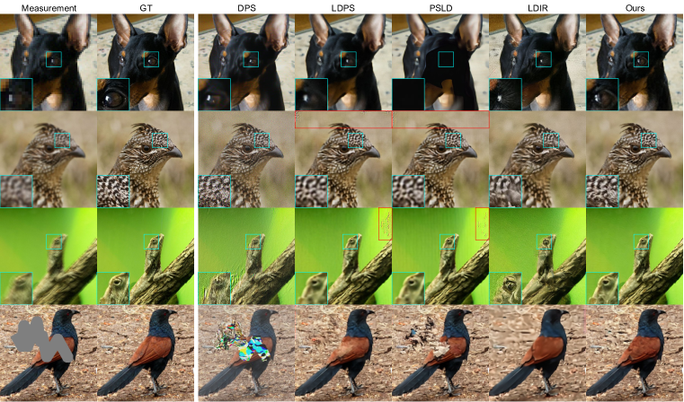
Figure 2: Inverse problem solving results on ImageNet $512\times 512$ test set. Row 1: SR$\times 8$, Row 2: gaussian deblurring, Row 3: motion deblurring, row 4: inpainting.

	SR ($\times 8$)			Deblur (motion)			Deblur (gauss)			Inpaint
Method	FID$\downarrow$	LPIPS$\downarrow$	PSNR$\uparrow$	FID$\downarrow$	LPIPS$\downarrow$	PSNR$\uparrow$	FID$\downarrow$	LPIPS$\downarrow$	PSNR$\uparrow$	FID$\downarrow$	LPIPS$\downarrow$	PSNR$\uparrow$
P2L (ours)	51.81	0.386	23.38	54.11	0.360	24.79	39.10	0.325	25.11	32.82	0.229	21.99
LDPS	61.09	0.475	23.21	71.12	0.441	23.32	48.17	0.392	24.91	46.72	0.332	21.54
GML-DPS (rout2023solving)	60.36	0.456	23.21	59.08	0.403	24.35	45.33	0.377	25.44	47.30	0.294	21.12
PSLD (rout2023solving)	60.81	0.471	23.17	59.63	0.398	24.21	45.44	0.376	25.42	40.57	0.251	20.92
LDIR (he2023iterative)	63.46	0.480	22.23	88.51	0.475	21.37	72.10	0.506	22.45	50.65	0.313	23.28
DDS (chung2023fast)	203.2	1.213	12.72	84.67	0.925	14.52	70.51	0.835	16.58	60.18	0.354	17.03
DPS (chung2023diffusion)	54.61	0.544	20.70	71.99	0.599	19.62	98.33	0.910	15.05	71.70	0.360	15.15
DiffPIR (zhu2023denoising)	488.3	1.182	13.44	87.04	0.622	19.32	79.31	0.755	20.55	45.97	0.300	20.11

Table 3: Quantitative evaluation (PSNR, LPIPS, FID) of inverse problem solving on ImageNet 512$\times$512-1k validation dataset. Bold: best, underline: second best. Methods that are not LDM-based are shaded in gray.

4.2 Main results

Comparison against baseline

In all of the inverse problems that we consider in the paper, our method outperforms all the baselines by quite a large margin in terms of perceptual quality, measured by FID and LPIPS, while keeping the distortion at a comparable level against the current state-of-the-art methods. Especially, we see about 10 FID decrease in deblurring and inpainting tasks compared to the runner up in both FFHQ and ImageNet dataset (See Tables 2,3). The superiority can also be clearly seen in Fig. 2, where P2L achieves stable, high-quality reconstruction throughout all tasks. Results from both LDPS and PSLD often contain local grid-like artifacts (Red boxes in Figures) and are blurry. With P2L, the restored images are sharpened while the artifacts are effectively removed. LDIR are less prone to artifacts owing to the smoothed history gradient updates, but often results in unrealistic textures and deviations from the measurement, which is also reflected in having the lowest PSNR among the LDIS-class methods. In contrast, P2L is free from such drawbacks even when leveraging Adam-like gradient update steps.

One rather surprising finding is the heavy downgrade in the performance for DIS methods. Even on in-distribution ImageNet test data, methods such as DPS and DiffPIR become very unstable. This can be attributed to the generative prior being poor: directly training diffusion models on high-resolution images often result in poor performance. This observation again points to the importance of developing methods that can leverage foundation models when aiming for general domain higher-resolution data. See Appendix E for further results. As a final note, we believe that the compromise in PSNR is related to the imperfectness of the VAE used in SD v1.4, and we expect such degradation to be mitigated when switching to better, larger autoencoders such as SDXL (podell2023sdxl).

Design components

			FFHQ				ImageNet
Design components			SR$\times 8$		Inpaint ($p=0.8$)		SR$\times 8$		Inpaint ($p=0.8$)
Projection	$\bm{\Gamma}$	Prompt tuning	FID$\downarrow$	PSNR$\uparrow$	FID$\downarrow$	PSNR$\uparrow$	FID$\downarrow$	PSNR$\uparrow$	FID$\downarrow$	PSNR$\uparrow$
✗	✗	✗	61.16	26.49	52.34	29.78	78.68	23.49	70.87	26.20
✗	✗	✓	58.73	26.68	51.40	29.69	76.40	23.52	67.06	26.32
✓	✗	✗	55.91	26.37	48.71	29.68	74.22	23.16	66.92	26.08
✓	✓	✗	55.68	26.43	47.76	29.70	74.01	23.32	65.45	26.29
✓	✓	✓	52.96	26.64	46.92	29.63	70.08	23.48	59.26	26.12

Table 4: Ablation studies on the design components

$\sigma_{y}$	$\bm{\Gamma}$	PSNR	FID
0.0	glue	26.51	54.69
	Ours	26.80	54.58
0.01	glue	26.39	56.47
	Ours	26.43	55.68
0.05	glue	23.86	68.99
	Ours	24.92	65.90

Table 5: Choice of $\bm{\Gamma}$

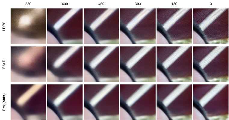
Figure 4: Close-up of the progress of ${\mathcal{D}}(\hat{\boldsymbol{z}}_{0})$ through time $t$ when solving $\times 8$ SR on FFHQ.

In Table 5, we perform an ablation study on the design components of the proposed method. From the table, we confirm that prompt tuning, projection to the range space of the encoder, and performing proximal update step (denoted as $\bm{\Gamma}$) before the projection all contributes to the gain in the performance. It is important that these gains are synergistic, and one component does not hamper the other. In the Appendix Tab. 7, we further show that our prompt-tuning approach is robust to the variation in the hyper-parameters (learning rate, number of iterations). Specifically, among the 9 configurations that we try, only the one with 5 iterations, lr=0.001 is inferior to not using prompt tuning. In Fig. 4, we visualize the progress of ${\mathcal{D}}(\hat{\boldsymbol{z}}_{0})$ through time $t$ starting from the same random seed, comparing LDPS, PSLD, and LDPS + projection (row 4 of Tab. 6). Here, we see that our proposed projection approach effectively suppresses the artifacts that arise during the reconstruction process, whereas PSLD introduces additional artifacts.

Choice of $\bm{\Gamma}$

When projecting to the range space of ${\mathcal{E}}$, we choose to use the proximal optimization strategy in Eq. (16). Instead, one could resort to projection to the measurement subspace (“gluing” of rout2023solving) by using $\bm{\Gamma}(\hat{\boldsymbol{x}}_{0})={\boldsymbol{A}}^{\top}{\boldsymbol{y}}+({\bm{I}}-{\boldsymbol{A}}^{\top}{\boldsymbol{A}})\hat{\boldsymbol{x}}_{0}$. In Table 5, we compare our choice of $\bm{\Gamma}$ against the gluing on various noise levels on FFHQ SR$\times 8$. We see that for all noise levels, the proximal steps consistently outperform the gluing, even when $\bm{\Gamma}$ is applied every $\gamma=4$ steps of reverse diffusion. Furthermore, due to the noise-amplifying nature of projection, the differences become more pronounced as we increase the noise level.

Figure 3: Results on $\times 8$ SR on DIV2K validation set of 768$\times$768 resolution. [Diffusion NFE per denoising step]. Vanilla and proposed process the latent as a whole.

High-resolution restoration

In Fig. 3, we show the effectiveness of our projection method on arbitrary resolution image restoration by comparing our method to bar2023multidiffusion and jimenez2023mixture, as well as the case where the larger latents are processed as a whole without patching (denoted as vanilla). Here, we see that the proposed method provides the best result, even when we use 1 NFE per denoising step, in contrast to requiring 4 NFE per denoising in the comparison methods. Further details and discussion is provided in Appendix D.

5 Conclusion

We proposed P2L, a latent diffusion model-based inverse problem solver that introduces two new strategies. First, a prompt tuning method to optimize the continuous input text embedding used for diffusion models was developed. We observed that our strategy can boost the performance by a good margin compared to the usage of null text embedding that prior works employ. Second, a projection approach to keep the latents in the range space of the encoder during the reverse diffusion process was proposed. Our approach effectively mitigated the artifacts that often arise during inverse problem solving, while also sharpening the final output. P2L outperforms previous diffusion model-based inverse problem solvers that operate on the latent and the image domain.

Limitations

While prompt tuning enhances the performance, it also incurs additional computational complexity as additional forward/backward passes through the latent diffusion model and the decoder is necessary. Consequently, the method will need future investigations when aiming for time-critical applications. As we optimize the continuous text embeddings rather than the discrete text directly, it is hard to decipher what the text embedding after the optimization has converged to. This is a limitation of the text embedder used for SD, as CLIP does not utilize a decoder. We could instead opt for the use of Imagen (saharia2022photorealistic), where T-5 with an encoder-decoder architecture is used, where one could easily check the learned text from our prompt-tuning scheme. Moreover, we did not consider the usage of CFG, which would enable flexible control on the degree of sharpening. Extending the prompt tuning idea to jointly optimize the embedding of the conditional and the unconditional model may be an interesting direction of future research.

Ethics statement

While our method can lead to advancements in areas such as computational imaging, medical imaging, and other fields where inverse problems are prevalent, we also recognize the potential for misuse in areas like deepfake generation or unauthorized data reconstruction, naturally leading from the use of generative models. The potential bias within the training dataset of the diffusion model may be potentially amplified with the usage of our method. We have taken care to ensure that our experiments adhere to ethical guidelines, using publicly available datasets or those for which we have obtained explicit permissions. We urge the community to adopt responsible practices when applying our findings and to consider the broader societal implications of the technology.

Reproducibility statement

In order to facilitate reproducibility, We detail our implementation in the form of Algorithms (Alg. 3,4,5), and pseudo-code (Fig. 5). The specific hyper-parameters chosen for the method is detailed in Appendix B.

Appendix A Proof-of-concept experiment

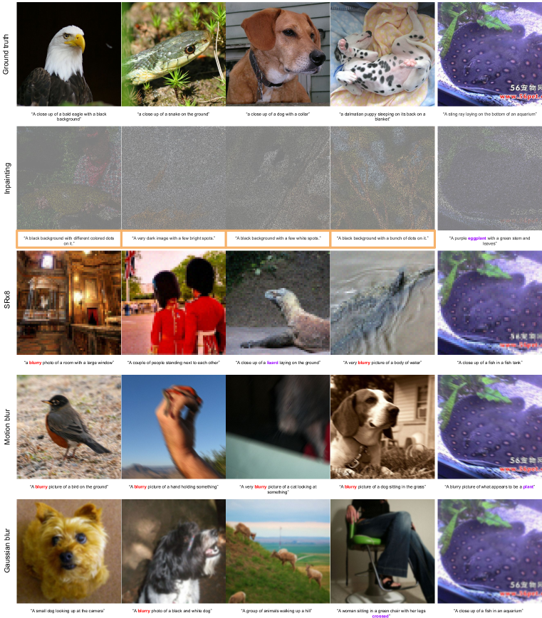
Figure 8: Captions generated by PALI (chen2022pali) from ground-truth ImageNet 512$\times$512 clean images, and the degraded images. The rightmost column contain images that are from the same ground truth. Captions in in orange box completely fail to describe the underlying image. Purple captions wrongly identify the image. Captions generated from degraded measurements often contain negative words such as blurry.

For the caption generation with PALI, we simply take the captions with the highest score. Examples of the captions generated from PALI are presented in Fig. 8. In our initial experiments, we found that using PALI captions directly did not directly lead to an improvement in the performance, as it only describes the content of the image, and says nothing about the quality of the image. Therefore, we use the following text prompts for the oracle “A high quality photo of a {PALI_prompt}”, similar to the general text prompts.

For both inverse problems (SR$\times 8$, inpainting with $p=0.8$), we use the LDPS algorithm with 1000 NFE and $\eta=0.0$. We apply prompt tuning algorithm per denoising step as indicated in Algorithm 3, with $K=5$ and learning rate of $1e-4$. When optimizing for the text embedding, we initialize it with the embedding vector from the token “A high quality photo of a face” for FFHQ, and “A high quality photo” for ImageNet in the case of inpainting. Note that for the latter, we did not find much performance difference when initializing from the null text prompt, or even initializing it with “A high quality photo of a dog”. For $\times 8$ SR, we initialize the text embeddings from PALI captions generated from ${\boldsymbol{y}}$, as we empirically observe that PALI captions from ${\boldsymbol{y}}$ still have a relatively good coarse description about the given image.

Appendix B Implementation details

	FFHQ				ImageNet
problem	Deblur (motion)	Deblur (gauss)	SR$\times 8$	inpaint	Deblur (motion)	Deblur (gauss)	SR$\times 8$	inpaint
Gradient type	Adam	Adam	GD	Adam	Adam	GD	GD	GD
$\rho_{t}$	0.05	0.05	1.0	0.05	0.1	$\bar{\alpha}_{t}$	$15\bar{\alpha}_{t}$	0.5
$\gamma$	5	4	4	3	5	4	4	3
$\lambda$	1.0	1.0	1.0	0.1	1.0	1.0	1.0	0.1
$K$	3	5	5	1	3	3	3	1
learning rate	$5e-5$	$1e-4$	$1e-4$	$1e-4$	$1e-5$	$1e-4$	$1e-5$	$1e-4$

Table 6: Hyper-parameter choice for the proposed method. White shade: hyper-parameters related to gradient updates, blue shade: hyper-parameters related to projecting onto the range space of ${\mathcal{E}}$, red shade: hyper-parameters related to prompt tuning.

B.1 Step 1: ${\mathcal{C}}$ update prompt tuning

Since we do not have the ground truth clean image to optimize the conditional embedding over, we use the following optimization strategy

$${\mathcal{C}}^{*}=\operatorname*{arg\,min}_{{\mathcal{C}}}\|{\boldsymbol{A}}{\mathcal{D}}\left({\mathbb{E}}[{\boldsymbol{z}}_{0}|{\boldsymbol{z}}_{t},{\boldsymbol{y}}]\right)-{\boldsymbol{y}}\|_{2}^{2},$$ (17)

where Eq. (17) is performed for every timestep $t$ during the inference stage. Here, we approximate the conditional posterior mean as

$${\mathbb{E}}[{\boldsymbol{z}}_{0}|{\boldsymbol{z}}_{t},{\boldsymbol{y}}] =\frac{1}{\sqrt{\bar{\alpha}_{t}}}{\boldsymbol{z}}_{t}+\frac{1-\bar{\alpha}_{t}}{\sqrt{\bar{\alpha}_{t}}}\left(\nabla_{{\boldsymbol{z}}_{t}}\log p({\boldsymbol{z}}_{t})+\nabla_{{\boldsymbol{z}}_{t}}\log p({\boldsymbol{y}}|{\boldsymbol{z}}_{t})\right)$$ (18)

$$\simeq{\mathbb{E}}[{\boldsymbol{z}}_{0}|{\boldsymbol{z}}_{t}]+\frac{1-\bar{\alpha}_{t}}{\sqrt{\bar{\alpha}_{t}}}\nabla_{\hat{\boldsymbol{z}}_{0|t}}\log p({\boldsymbol{y}}|\hat{\boldsymbol{z}}_{0|t}),$$ (19)

which is the result of the approximations proposed in (ravula2023optimizing; barbano2023steerable). In practice, we choose a static step size $\rho=1.0$ with the gradient of the norm, which was shown to be effective in (chung2023diffusion). The resulting prompt tuning algorithm is summarized in Algorithm 3. Notice that we update our embeddings to improve the fidelity Eq. (17). However, in practice, this also leads to higher quality images in terms of perception. For optimizing Eq. (17), we use Adam with the learning rate and the number of iterations as denoted in Table 6 for every $t$.

Algorithm 5 P2L: Adam

1:${\boldsymbol{\epsilon}}_{{\boldsymbol{\theta}}^{*}},{\boldsymbol{z}}_{T},{\boldsymbol{y}},{\mathcal{C}},T,K,\gamma,\beta_{1},\beta_{2},\varepsilon,\bm{\Gamma}$

2:$\bm{m}_{T}\leftarrow$ np.zeros_like$({{\boldsymbol{z}}_{T}})$

3:$\bm{v}_{T}\leftarrow$ np.zeros_like$({{\boldsymbol{z}}_{T}})$

4:for $t=T$ to $1$ do

5:     ${\mathcal{C}}_{t}^{*}\leftarrow\color[rgb]{0,0,0}{\textsc{OptimizeEmb}}({\boldsymbol{z}}_{t},{\boldsymbol{y}},{\mathcal{C}}_{t}^{0})$

6:     $\hat{\boldsymbol{\epsilon}}_{t}\leftarrow{\boldsymbol{\epsilon}}_{{\boldsymbol{\theta}}^{*}}({\boldsymbol{z}}_{t},{\mathcal{C}}_{t}^{*})$

7:     $\hat{\boldsymbol{z}}_{0|t}\leftarrow({\boldsymbol{z}}_{t}-\sqrt{1-\bar{\alpha}_{t}}\hat{{\boldsymbol{\epsilon}}}_{t}){/\sqrt{\bar{\alpha}_{t}}}$

8:     if $(t\mod\gamma)=0$ then

9:         $\color[rgb]{0,0,0}{\hat{\boldsymbol{z}}^{\prime}_{0|t}\leftarrow{\mathcal{E}}\left({\bm{\Gamma}}\left({\mathcal{D}}(\hat{\boldsymbol{z}}_{0|t})\right)\right)}$

10:     end if

11:     ${\boldsymbol{z}}^{\prime}_{t-1}\leftarrow\sqrt{\bar{\alpha}_{t-1}}\hat{\boldsymbol{z}}^{\prime}_{0|t}+\sqrt{1-\bar{\alpha}_{t-1}}\hat{\boldsymbol{\epsilon}}_{t}$

12:     ${\boldsymbol{g}}\leftarrow\nabla_{{\boldsymbol{z}}_{t}}\|{\mathcal{A}}{\mathcal{D}}(\hat{\boldsymbol{z}}_{0|t})-{\boldsymbol{y}}\|$

13:     $\hat{\bm{m}}_{t-1}\leftarrow\left(\beta_{1}\bm{m}_{t}+(1-\beta_{1}){\boldsymbol{g}}\right)/(1-\beta_{1})$

14:     $\hat{\bm{v}}_{t-1}\leftarrow\left(\beta_{2}\bm{v}_{t}+(1-\beta_{2})({\boldsymbol{g}}\circ{\boldsymbol{g}})\right)/(1-\beta_{2})$

15:     ${\boldsymbol{z}}_{t-1}\leftarrow{\boldsymbol{z}}^{\prime}_{t-1}-\rho_{t}\frac{\hat{\bm{m}}_{t-1}}{\sqrt{\hat{\bm{v}}_{t-1}}+\varepsilon}$

16:     ${\mathcal{C}}_{t-1}^{(0)}\leftarrow{\mathcal{C}}_{t}^{*}$

17:end for

18:return ${\boldsymbol{x}}_{0}\leftarrow{\mathcal{D}}({\boldsymbol{z}}_{0})$

B.2 Step 2: ${\boldsymbol{z}}_{t}$ update

In Table 6, there are two gradient types: GD and Adam. For GD, we use standard gradient descent steps as presented in Algorithm 4. For Adam, using the same prompt tuning Algorithm 3, we adopt a history gradient update scheme as proposed in he2023iterative to arrive at Algorithm 5. Note that the hyper-parameters of the Adam update were fixed to be $\beta_{1}=0.9,\beta_{2}=0.999,\varepsilon=1e-8$, which is the default setting. We only search for the optimal step size $\rho_{t}$ via grid search, which is set to 0.1 for motion deblurring in ImageNet, and 0.05 otherwise.

B.3 Comparison methods

LDPS

LDPS can be considered a straightforward extension image domain DPS (chung2023diffusion). The three works that we review in this section (he2023iterative; rout2023solving; song2023solving) all consider LDPS as a baseline. In LDPS, we have the following update scheme

$${\boldsymbol{z}}_{t-1} ={\rm DDIM}({\boldsymbol{z}}_{t})-\rho\nabla_{{\boldsymbol{z}}_{t}}\|{\boldsymbol{y}}-{\boldsymbol{A}}{\mathcal{D}}(\hat{\boldsymbol{z}}_{0})\|_{2},$$ (20)

where $\rho$ is the step size, and ${\rm DDIM}(\cdot)$ denotes a single step of DDIM sampling. We use a static step size of $\rho=1$, widely adopted in literature.

LDIR (he2023iterative)

Using Adam-like history gradient update scheme, a single iteration of the algorithm can be summarized as follows

$${\boldsymbol{g}}_{t} =\nabla_{{\boldsymbol{z}}_{t}}\|{\boldsymbol{y}}-{\boldsymbol{A}}{\mathcal{D}}(\hat{\boldsymbol{z}}_{0})\|$$ (21)

$$\hat{\boldsymbol{m}}_{t} =(\beta_{1}{\boldsymbol{m}}_{t-1}+(1-\beta_{1}){\boldsymbol{g}}_{t})/(1-\beta_{1})$$ (22)

$$\hat{\bm{v}}_{t} =(\beta_{2}{\bm{v}}_{t-1}+(1-\beta_{2})({\boldsymbol{g}}_{t}\circ{\boldsymbol{g}}_{t}))/(1-\beta_{2})$$ (23)

$${\boldsymbol{z}}_{t-1} ={\rm DDIM}({\boldsymbol{z}}_{t})-\rho\frac{\hat{\boldsymbol{m}}_{t}}{\sqrt{\hat{\bm{v}}_{t}}+\varepsilon},$$ (24)

where $\circ$ denotes element-wise product, and $\beta_{1},\beta_{2},\varepsilon$ are the hyperparameters of the sampling scheme. As LDIR uses a momentum-based update scheme, we have smoother gradient transitions. We fix $\beta_{1}=0.9,\beta_{2}=0.999,\varepsilon=1e-8$ to be identical to when using the proposed method. The step size $\rho$ is chosen to be the optimal value found through grid search: 0.1 for ImageNet motion deblurring, and 0.05 otherwise.

GML-DPS, PSLD (rout2023solving)

GML-DPS attempts to regularize the predicted clean latent $\hat{\boldsymbol{z}}_{0}$ to be a fixed point after encoding and decoding. Formally, the update step reads

$${\boldsymbol{z}}_{t-1} ={\rm DDIM}({\boldsymbol{z}}_{t})-\rho\nabla_{{\boldsymbol{z}}_{t}}\left(\|{\boldsymbol{y}}-{\boldsymbol{A}}{\mathcal{D}}(\hat{\boldsymbol{z}}_{0})\|_{2}+\gamma\|\hat{\boldsymbol{z}}_{0}-{\mathcal{E}}({\mathcal{D}}(\hat{\boldsymbol{z}}_{0}))\|_{2}\right).$$ (25)

Further, PSLD applies an orthogonal projection onto the subspace of ${\boldsymbol{A}}$ in between decoding and encoding to enforce fidelity

$${\boldsymbol{z}}_{t-1} ={\rm DDIM}({\boldsymbol{z}}_{t})-\rho\nabla_{{\boldsymbol{z}}_{t}}\left(\|{\boldsymbol{y}}-{\boldsymbol{A}}{\mathcal{D}}(\hat{\boldsymbol{z}}_{0})\|_{2}+\gamma\|\hat{\boldsymbol{z}}_{0}-{\mathcal{E}}({\boldsymbol{A}}^{\top}{\boldsymbol{y}}+({\bm{I}}-{\boldsymbol{A}}^{\top}{\boldsymbol{A}}){\mathcal{D}}(\hat{\boldsymbol{z}}_{0}))\|_{2}\right).$$ (26)

We use the static step size of $\rho=1$, and choose $\gamma=0.1$, as advised in rout2023solving. GML-DPS and PSLD are closest to the proposed method in spirit, as these methods attempt to guide the latents to stay closer to the natural manifold by enforcing them to be a fixed point after autoencoding. The difference is that these approaches use gradient guidance while we try to explicitly project the latents into the the natural manifold.

DPS (chung2023diffusion)

DPS is a DIS that utilizes the following update scheme

$${\boldsymbol{x}}_{t-1} ={\rm DDIM}({\boldsymbol{x}}_{t})-\nabla_{{\boldsymbol{x}}_{t}}\left(\|{\boldsymbol{y}}-{\boldsymbol{A}}\hat{\boldsymbol{x}}_{0}\|_{2}\right).$$ (27)

The optimal value of $\eta$ was found through grid search for each inverse problem: $\eta=0.0$ for SR$\times 8$, and $\eta=1.0$ for others.

DDS (chung2023fast)

The following updates are used

$$\hat{\boldsymbol{x}}^{\prime}_{0} =\operatorname*{arg\,min}_{\boldsymbol{x}}\frac{1}{2}\|{\boldsymbol{y}}-{\boldsymbol{A}}{\boldsymbol{x}}\|_{2}^{2}+\frac{\gamma}{2}\|{\boldsymbol{x}}-\hat{\boldsymbol{x}}_{0}\|_{2}^{2}$$ (28)

$${\boldsymbol{x}}_{t-1} =\sqrt{\bar{\alpha}_{t-1}}\hat{\boldsymbol{x}}^{\prime}_{0}+\sqrt{1-\bar{\alpha}_{t-1}-\eta^{2}\tilde{\beta}_{t-1}^{2}}\hat{\boldsymbol{\epsilon}}_{t}+\eta\tilde{\beta}_{t-1}{\boldsymbol{\epsilon}},$$ (29)

where Eq. (28) is solved through CG with 5 iterations, $\gamma=1.0$. $\eta=0.0$ is chosen for Gaussian deblurring, and $\eta=1.0$ for the rest of the inverse problems.

DiffPIR (zhu2023denoising)

Similar to DDS, the following updates are used

$$\hat{\boldsymbol{x}}^{\prime}_{0} =\operatorname*{arg\,min}_{\boldsymbol{x}}\frac{1}{2}\|{\boldsymbol{y}}-{\boldsymbol{A}}{\boldsymbol{x}}\|_{2}^{2}+\frac{\lambda\sigma^{2}\bar{\alpha}_{t}}{2(1-\bar{\alpha}_{t})}\|{\boldsymbol{x}}-\hat{\boldsymbol{x}}_{0}\|_{2}^{2}$$ (30)

$${\boldsymbol{x}}_{t-1} =\sqrt{\bar{\alpha}_{t-1}}\hat{\boldsymbol{x}}^{\prime}_{0}+\sqrt{1-\bar{\alpha}_{t-1}}(\sqrt{1-\zeta}\hat{\boldsymbol{\epsilon}}_{t}+\sqrt{\zeta}{\boldsymbol{\epsilon}}),$$ (31)

where $\sigma$ is the noise level of the measurement, and $\lambda,\zeta$ are hyper-parameters. Unlike DDS, the solution to Eq. (30) is obtained as a closed-form solution. These hyper-parameters are found through grid search. SR$\times 8$: $\zeta=0.35,\lambda=35.0$ / Deblur: $\zeta=0.3,\lambda=7.0$ / Inpaint: $\zeta=1.0/\lambda=7.0$.

steps	$0$	$1$			$3$			$5$
lr	-	$1e-5$	$1e-4$	$1e-3$	$1e-5$	$1e-4$	$1e-3$	$1e-5$	$1e-4$	$1e-3$
FID	61.16	60.66	59.60	57.61	60.11	59.34	60.19	60.02	58.59	62.67
PSNR	26.49	26.69	26.71	26.73	26.78	26.70	26.61	26.73	26.17	26.38

Table 7: Robustness to hyper-parameters in prompt-tuning. FFHQ SR$\times 8$ on 256 test images. Bold: best, underline: second best.

Appendix C Efficient implementation in JAX

⬇

ones = jnp.ones(x.shape)

_, _AT = jax.vjp(A_funcs.A, ones)

AT = lambda y: _AT(y)[0]

A_funcs.AT = AT

def cg_A(x, cg_lamb):

return A_funcs.AT(A_funcs.A(x)) + cg_lamb * x

hatx0 = D(hatz0)

cg_y = A_funcs.AT(y) + cg_lamb * hatx0

hatx0, _ = jax.scipy.sparse.linalg.cg(cg_A, cg_y, x0=hatx0)

Figure 5: Defining ${\boldsymbol{A}}^{\top}$ can be automatically achieved through jax.vjp given that ${\boldsymbol{A}}$ is differentiable.

In model-based inverse problem solving, having access to efficient computation of the adjoint ${\boldsymbol{A}}^{\top}$ is a must. Here, we consider a general case of solving linear inverse problems where the computation of SVD is too costly, and hence one has to define the adjoint operator manually (e.g. computed tomography). Furthermore, for cases such as deblurring from circular convolution, one needs to carefully design the operator, as there are many potential pitfalls (e.g. boundary, size mismatch). These are more often than not the limiting factors of the applicability of the model-based approaches for solving inverse problems. We show in Fig. 5 that this can be much alleviated by using jax, as we can implicitly define a transpose operator with reverse-mode automatic differentiation (baydin2018automatic). We note this design was also established in (scico-2022).

Appendix D Targetting arbitrary resolution

For SD, using an encoder to convert from the image to the latent space reduces the dimension by $\times 8$. When training SD, the diffusion model that operates on the latent space was trained with 64$\times$64 latents, obtained from 512$\times$512 images. When the image that we wish to restore (or generate) is larger than 512$\times$512, the latents will also be larger than 64$\times$64. In this case, due to the train-test time discrepancy, the results that we get will be suboptimal if one processes the larger latent as a whole (Fig. 6 (a)). A natural way to counteract this discrepancy is to process the latents in patches. When processing in patches of size 64$\times$64 with stride 32 on both directions, it requires us 4 score function NFEs per denoising step (Fig. 6 (b),(c)). bar2023multidiffusion uniformly weights the overlapping patches, and jimenez2023mixture weights the patches with Gaussian weights with variance 0.01. The downside of these methods is that the number NFEs required for inference scales quadratically with the size of the image.

On the other hand, the proposed method can process the large latent as a whole, as in the “vanilla” method, and project this latent to the range space of ${\mathcal{E}}$ by setting $\hat{\boldsymbol{z}}^{\prime}_{0}={\mathcal{D}}(\bm{\Gamma}({\mathcal{E}}(\hat{\boldsymbol{z}}_{0})))$ for every few steps. Even though the proposed method is considerably faster than patch-based methods (bar2023multidiffusion; jimenez2023mixture), we see that one can achieve a comparable, or superior performance, as presented in Fig. 3. Furthermore, in Fig. 7, we show that we can use both patching method and the projection method simultaneously, achieving the best results.

Figure 6: Method comparison for processing higher resolution images in the latent space.

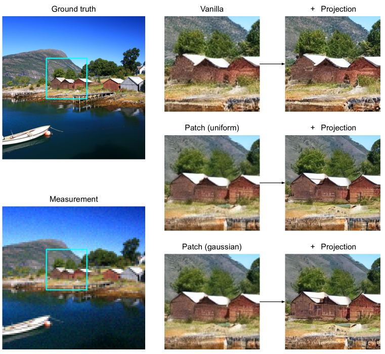
Figure 7: Further results on $\times 8$ SR on DIV2K validation set of 768$\times$768 resolution. Comparison between with and without using our projection approach on various baseline methods.

Appendix E Further experimental results

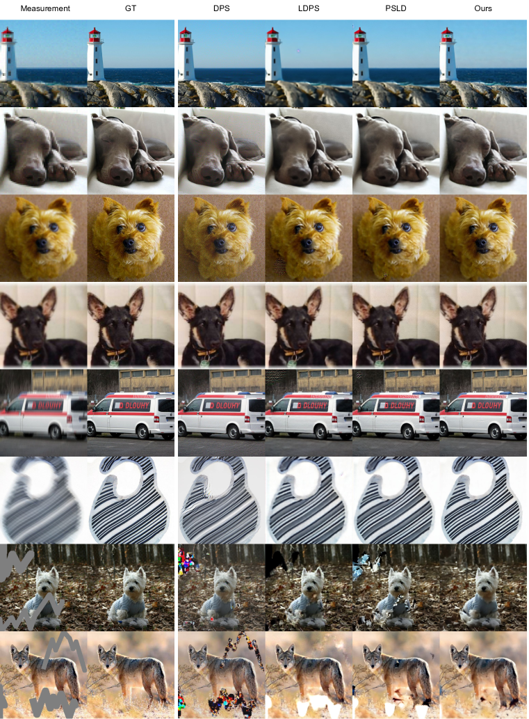
Figure 9: ImageNet restoration results. Row 1-2: SR$\times 8$, row 3-4: gaussian deblurring, row 5-6: motion deblurring, row 7-8: freeform inpainting; All with $\sigma=0.01$ noise.

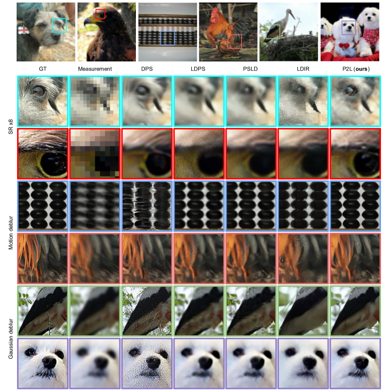
Figure 10: Close-up comparison on diverse inverse problem tasks. Ground truth, measurement, DPS (chung2023diffusion), LDPS, PSLD (rout2023solving), LDIR (he2023iterative), and the proposed method.

References

- Balke et al. (2022) Thilo Balke, Fernando Davis, Cristina Garcia-Cardona, Michael McCann, Luke Pfister, and Brendt Wohlberg. Scientific Computational Imaging COde (SCICO). Software library available from https://github.com/lanl/scico, 2022.
- Bar-Tal et al. (2023) Omer Bar-Tal, Lior Yariv, Yaron Lipman, and Tali Dekel. Multidiffusion: Fusing diffusion paths for controlled image generation. 2023.
- Barbano et al. (2023) Riccardo Barbano, Alexander Denker, Hyungjin Chung, Tae Hoon Roh, Simon Arrdige, Peter Maass, Bangti Jin, and Jong Chul Ye. Steerable conditional diffusion for out-of-distribution adaptation in imaging inverse problems. arXiv preprint arXiv:2308.14409, 2023.
- Baydin et al. (2018) Atilim Gunes Baydin, Barak A Pearlmutter, Alexey Andreyevich Radul, and Jeffrey Mark Siskind. Automatic differentiation in machine learning: a survey. Journal of Marchine Learning Research, 18:1–43, 2018.
- Blau & Michaeli (2018) Yochai Blau and Tomer Michaeli. The perception-distortion tradeoff. In Proceedings of the IEEE conference on computer vision and pattern recognition, pp. 6228–6237, 2018.
- Bora et al. (2017) Ashish Bora, Ajil Jalal, Eric Price, and Alexandros G Dimakis. Compressed sensing using generative models. In International conference on machine learning, pp. 537–546. PMLR, 2017.
- Brock et al. (2018) Andrew Brock, Jeff Donahue, and Karen Simonyan. Large scale gan training for high fidelity natural image synthesis. arXiv preprint arXiv:1809.11096, 2018.
- Brown et al. (2020) Tom Brown, Benjamin Mann, Nick Ryder, Melanie Subbiah, Jared D Kaplan, Prafulla Dhariwal, Arvind Neelakantan, Pranav Shyam, Girish Sastry, Amanda Askell, et al. Language models are few-shot learners. Advances in neural information processing systems, 33:1877–1901, 2020.
- Chen et al. (2022) Xi Chen, Xiao Wang, Soravit Changpinyo, AJ Piergiovanni, Piotr Padlewski, Daniel Salz, Sebastian Goodman, Adam Grycner, Basil Mustafa, Lucas Beyer, et al. Pali: A jointly-scaled multilingual language-image model. arXiv preprint arXiv:2209.06794, 2022.
- Chung & Ye (2022) Hyungjin Chung and Jong Chul Ye. Score-based diffusion models for accelerated mri. Medical Image Analysis, pp. 102479, 2022.
- Chung et al. (2023a) Hyungjin Chung, Jeongsol Kim, Sehui Kim, and Jong Chul Ye. Parallel diffusion models of operator and image for blind inverse problems. IEEE/CVF Conference on Computer Vision and Pattern Recognition, 2023a.
- Chung et al. (2023b) Hyungjin Chung, Jeongsol Kim, Michael Thompson Mccann, Marc Louis Klasky, and Jong Chul Ye. Diffusion posterior sampling for general noisy inverse problems. In International Conference on Learning Representations, 2023b. URL https://openreview.net/forum?id=OnD9zGAGT0k.
- Chung et al. (2023c) Hyungjin Chung, Suhyeon Lee, and Jong Chul Ye. Fast diffusion sampler for inverse problems by geometric decomposition. arXiv preprint arXiv:2303.05754, 2023c.
- Chung et al. (2023d) Hyungjin Chung, Dohoon Ryu, Michael T Mccann, Marc L Klasky, and Jong Chul Ye. Solving 3d inverse problems using pre-trained 2d diffusion models. IEEE/CVF Conference on Computer Vision and Pattern Recognition, 2023d.
- Daras et al. (2022) Giannis Daras, Yuval Dagan, Alexandros G Dimakis, and Constantinos Daskalakis. Score-guided intermediate layer optimization: Fast langevin mixing for inverse problem. arXiv preprint arXiv:2206.09104, 2022.
- Delbracio & Milanfar (2023) Mauricio Delbracio and Peyman Milanfar. Inversion by direct iteration: An alternative to denoising diffusion for image restoration. arXiv preprint arXiv:2303.11435, 2023.
- Deng et al. (2009) Jia Deng, Wei Dong, Richard Socher, Li-Jia Li, Kai Li, and Li Fei-Fei. Imagenet: A large-scale hierarchical image database. In 2009 IEEE conference on computer vision and pattern recognition, pp. 248–255. Ieee, 2009.
- Dhariwal & Nichol (2021) Prafulla Dhariwal and Alexander Quinn Nichol. Diffusion models beat GANs on image synthesis. In A. Beygelzimer, Y. Dauphin, P. Liang, and J. Wortman Vaughan (eds.), Advances in Neural Information Processing Systems, 2021.
- Efron (2011) Bradley Efron. Tweedie’s formula and selection bias. Journal of the American Statistical Association, 106(496):1602–1614, 2011.
- Feng et al. (2023) Berthy T Feng, Jamie Smith, Michael Rubinstein, Huiwen Chang, Katherine L Bouman, and William T Freeman. Score-based diffusion models as principled priors for inverse imaging. arXiv preprint arXiv:2304.11751, 2023.
- Gal et al. (2022) Rinon Gal, Yuval Alaluf, Yuval Atzmon, Or Patashnik, Amit H Bermano, Gal Chechik, and Daniel Cohen-Or. An image is worth one word: Personalizing text-to-image generation using textual inversion. arXiv preprint arXiv:2208.01618, 2022.
- Geman & Geman (1984) Stuart Geman and Donald Geman. Stochastic relaxation, gibbs distributions, and the bayesian restoration of images. IEEE Transactions on pattern analysis and machine intelligence, (6):721–741, 1984.
- González et al. (2022) Mario González, Andrés Almansa, and Pauline Tan. Solving inverse problems by joint posterior maximization with autoencoding prior. SIAM Journal on Imaging Sciences, 15(2):822–859, 2022.
- He et al. (2023) Linchao He, Hongyu Yan, Mengting Luo, Kunming Luo, Wang Wang, Wenchao Du, Hu Chen, Hongyu Yang, and Yi Zhang. Iterative reconstruction based on latent diffusion model for sparse data reconstruction. arXiv preprint arXiv:2307.12070, 2023.
- Hertz et al. (2022) Amir Hertz, Ron Mokady, Jay Tenenbaum, Kfir Aberman, Yael Pritch, and Daniel Cohen-Or. Prompt-to-prompt image editing with cross attention control. arXiv preprint arXiv:2208.01626, 2022.
- Ho & Salimans (2021) Jonathan Ho and Tim Salimans. Classifier-free diffusion guidance. In NeurIPS 2021 Workshop on Deep Generative Models and Downstream Applications, 2021. URL https://openreview.net/forum?id=qw8AKxfYbI.
- Ho et al. (2020) Jonathan Ho, Ajay Jain, and Pieter Abbeel. Denoising diffusion probabilistic models. Advances in Neural Information Processing Systems, 33:6840–6851, 2020.
- Ho et al. (2022) Jonathan Ho, William Chan, Chitwan Saharia, Jay Whang, Ruiqi Gao, Alexey Gritsenko, Diederik P Kingma, Ben Poole, Mohammad Norouzi, David J Fleet, et al. Imagen video: High definition video generation with diffusion models. arXiv preprint arXiv:2210.02303, 2022.
- Jiménez (2023) Álvaro Barbero Jiménez. Mixture of diffusers for scene composition and high resolution image generation. arXiv preprint arXiv:2302.02412, 2023.
- Kadkhodaie & Simoncelli (2021) Zahra Kadkhodaie and Eero Simoncelli. Stochastic solutions for linear inverse problems using the prior implicit in a denoiser. In Advances in Neural Information Processing Systems, volume 34, pp. 13242–13254. Curran Associates, Inc., 2021.
- Kamilov et al. (2023) Ulugbek S Kamilov, Charles A Bouman, Gregery T Buzzard, and Brendt Wohlberg. Plug-and-play methods for integrating physical and learned models in computational imaging: Theory, algorithms, and applications. IEEE Signal Processing Magazine, 40(1):85–97, 2023.
- Karras et al. (2019) Tero Karras, Samuli Laine, and Timo Aila. A style-based generator architecture for generative adversarial networks. In Proceedings of the IEEE/CVF Conference on Computer Vision and Pattern Recognition, pp. 4401–4410, 2019.
- Kawar et al. (2021) Bahjat Kawar, Gregory Vaksman, and Michael Elad. Snips: Solving noisy inverse problems stochastically. Advances in Neural Information Processing Systems, 34:21757–21769, 2021.
- Kawar et al. (2022) Bahjat Kawar, Michael Elad, Stefano Ermon, and Jiaming Song. Denoising diffusion restoration models. In Alice H. Oh, Alekh Agarwal, Danielle Belgrave, and Kyunghyun Cho (eds.), Advances in Neural Information Processing Systems, 2022. URL https://openreview.net/forum?id=kxXvopt9pWK.
- Kingma & Ba (2015) Diederik P. Kingma and Jimmy Ba. Adam: A method for stochastic optimization. In ICLR, 2015.
- Kingma & Welling (2013) Diederik P Kingma and Max Welling. Auto-encoding variational bayes. arXiv preprint arXiv:1312.6114, 2013.
- Kojima et al. (2022) Takeshi Kojima, Shixiang Shane Gu, Machel Reid, Yutaka Matsuo, and Yusuke Iwasawa. Large language models are zero-shot reasoners. Advances in neural information processing systems, 35:22199–22213, 2022.
- Laroche et al. (2023) Charles Laroche, Andrés Almansa, and Eva Coupete. Fast diffusion em: a diffusion model for blind inverse problems with application to deconvolution. arXiv preprint arXiv:2309.00287, 2023.
- Lee et al. (2023) Suhyeon Lee, Hyungjin Chung, Minyoung Park, Jonghyuk Park, Wi-Sun Ryu, and Jong Chul Ye. Improving 3D imaging with pre-trained perpendicular 2D diffusion models. arXiv preprint arXiv:2303.08440, 2023.
- Mardani et al. (2023) Morteza Mardani, Jiaming Song, Jan Kautz, and Arash Vahdat. A variational perspective on solving inverse problems with diffusion models. arXiv preprint arXiv:2305.04391, 2023.
- Mokady et al. (2023) Ron Mokady, Amir Hertz, Kfir Aberman, Yael Pritch, and Daniel Cohen-Or. Null-text inversion for editing real images using guided diffusion models. In Proceedings of the IEEE/CVF Conference on Computer Vision and Pattern Recognition, pp. 6038–6047, 2023.
- Murata et al. (2023) Naoki Murata, Koichi Saito, Chieh-Hsin Lai, Yuhta Takida, Toshimitsu Uesaka, Yuki Mitsufuji, and Stefano Ermon. Gibbsddrm: A partially collapsed gibbs sampler for solving blind inverse problems with denoising diffusion restoration. arXiv preprint arXiv:2301.12686, 2023.
- Ongie et al. (2020) Gregory Ongie, Ajil Jalal, Christopher A Metzler, Richard G Baraniuk, Alexandros G Dimakis, and Rebecca Willett. Deep learning techniques for inverse problems in imaging. IEEE Journal on Selected Areas in Information Theory, 1(1):39–56, 2020.
- Parikh & Boyd (2014) Neal Parikh and Stephen Boyd. Proximal algorithms. Foundations and Trends in optimization, 1(3):127–239, 2014.
- Podell et al. (2023) Dustin Podell, Zion English, Kyle Lacey, Andreas Blattmann, Tim Dockhorn, Jonas Müller, Joe Penna, and Robin Rombach. Sdxl: improving latent diffusion models for high-resolution image synthesis. arXiv preprint arXiv:2307.01952, 2023.
- Poole et al. (2023) Ben Poole, Ajay Jain, Jonathan T. Barron, and Ben Mildenhall. Dreamfusion: Text-to-3d using 2d diffusion. In The Eleventh International Conference on Learning Representations, 2023. URL https://openreview.net/forum?id=FjNys5c7VyY.
- Radford et al. (2021) Alec Radford, Jong Wook Kim, Chris Hallacy, Aditya Ramesh, Gabriel Goh, Sandhini Agarwal, Girish Sastry, Amanda Askell, Pamela Mishkin, Jack Clark, et al. Learning transferable visual models from natural language supervision. In International conference on machine learning, pp. 8748–8763. PMLR, 2021.
- Ramesh et al. (2022) Aditya Ramesh, Prafulla Dhariwal, Alex Nichol, Casey Chu, and Mark Chen. Hierarchical text-conditional image generation with clip latents. arXiv preprint arXiv:2204.06125, 1(2):3, 2022.
- Ravula et al. (2023) Sriram Ravula, Brett Levac, Ajil Jalal, Jonathan I Tamir, and Alexandros G Dimakis. Optimizing sampling patterns for compressed sensing mri with diffusion generative models. arXiv preprint arXiv:2306.03284, 2023.
- Robbins (1956) Herbert Robbins. An empirical bayes approach to statistics. In Proc. 3rd Berkeley Symp. Math. Statist. Probab., 1956, volume 1, pp. 157–163, 1956.
- Romano et al. (2017) Yaniv Romano, Michael Elad, and Peyman Milanfar. The little engine that could: Regularization by denoising (red). SIAM Journal on Imaging Sciences, 10(4):1804–1844, 2017.
- Rombach et al. (2022) Robin Rombach, Andreas Blattmann, Dominik Lorenz, Patrick Esser, and Björn Ommer. High-resolution image synthesis with latent diffusion models. In Proceedings of the IEEE/CVF Conference on Computer Vision and Pattern Recognition, pp. 10684–10695, 2022.
- Rout et al. (2023) Litu Rout, Negin Raoof, Giannis Daras, Constantine Caramanis, Alexandros G Dimakis, and Sanjay Shakkottai. Solving linear inverse problems provably via posterior sampling with latent diffusion models. arXiv preprint arXiv:2307.00619, 2023.
- Saharia et al. (2022a) Chitwan Saharia, William Chan, Huiwen Chang, Chris Lee, Jonathan Ho, Tim Salimans, David Fleet, and Mohammad Norouzi. Palette: Image-to-image diffusion models. In ACM SIGGRAPH 2022 Conference Proceedings, pp. 1–10, 2022a.
- Saharia et al. (2022b) Chitwan Saharia, William Chan, Saurabh Saxena, Lala Li, Jay Whang, Emily L Denton, Kamyar Ghasemipour, Raphael Gontijo Lopes, Burcu Karagol Ayan, Tim Salimans, et al. Photorealistic text-to-image diffusion models with deep language understanding. Advances in Neural Information Processing Systems, 35:36479–36494, 2022b.
- Schuhmann et al. (2022) Christoph Schuhmann, Romain Beaumont, Richard Vencu, Cade Gordon, Ross Wightman, Mehdi Cherti, Theo Coombes, Aarush Katta, Clayton Mullis, Mitchell Wortsman, et al. Laion-5b: An open large-scale dataset for training next generation image-text models. Advances in Neural Information Processing Systems, 35:25278–25294, 2022.
- Shin et al. (2020) Taylor Shin, Yasaman Razeghi, Robert L Logan IV, Eric Wallace, and Sameer Singh. Autoprompt: Eliciting knowledge from language models with automatically generated prompts. arXiv preprint arXiv:2010.15980, 2020.
- Sohl-Dickstein et al. (2015) Jascha Sohl-Dickstein, Eric Weiss, Niru Maheswaranathan, and Surya Ganguli. Deep unsupervised learning using nonequilibrium thermodynamics. In International Conference on Machine Learning, pp. 2256–2265. PMLR, 2015.
- Song et al. (2023a) Bowen Song, Soo Min Kwon, Zecheng Zhang, Xinyu Hu, Qing Qu, and Liyue Shen. Solving inverse problems with latent diffusion models via hard data consistency. arXiv preprint arXiv:2307.08123, 2023a.
- Song et al. (2023b) Jiaming Song, Arash Vahdat, Morteza Mardani, and Jan Kautz. Pseudoinverse-guided diffusion models for inverse problems. In International Conference on Learning Representations, 2023b. URL https://openreview.net/forum?id=9_gsMA8MRKQ.
- Song et al. (2021) Yang Song, Jascha Sohl-Dickstein, Diederik P. Kingma, Abhishek Kumar, Stefano Ermon, and Ben Poole. Score-based generative modeling through stochastic differential equations. In 9th International Conference on Learning Representations, ICLR, 2021.
- Song et al. (2022) Yang Song, Liyue Shen, Lei Xing, and Stefano Ermon. Solving inverse problems in medical imaging with score-based generative models. In International Conference on Learning Representations, 2022. URL https://openreview.net/forum?id=vaRCHVj0uGI.
- Venkatakrishnan et al. (2013) Singanallur V Venkatakrishnan, Charles A Bouman, and Brendt Wohlberg. Plug-and-play priors for model based reconstruction. In 2013 IEEE global conference on signal and information processing, pp. 945–948. IEEE, 2013.
- Vincent (2011) Pascal Vincent. A connection between score matching and denoising autoencoders. Neural computation, 23(7):1661–1674, 2011.
- Wang et al. (2023a) Jianyi Wang, Zongsheng Yue, Shangchen Zhou, Kelvin CK Chan, and Chen Change Loy. Exploiting diffusion prior for real-world image super-resolution. arXiv preprint arXiv:2305.07015, 2023a.
- Wang et al. (2023b) Yinhuai Wang, Jiwen Yu, Runyi Yu, and Jian Zhang. Unlimited-size diffusion restoration. In Proceedings of the IEEE/CVF Conference on Computer Vision and Pattern Recognition, pp. 1160–1167, 2023b.
- Wang et al. (2023c) Zhengyi Wang, Cheng Lu, Yikai Wang, Fan Bao, Chongxuan Li, Hang Su, and Jun Zhu. Prolificdreamer: High-fidelity and diverse text-to-3d generation with variational score distillation. arXiv preprint arXiv:2305.16213, 2023c.
- Whang et al. (2021) Jay Whang, Qi Lei, and Alex Dimakis. Solving inverse problems with a flow-based noise model. In International Conference on Machine Learning, pp. 11146–11157. PMLR, 2021.
- Whang et al. (2022) Jay Whang, Mauricio Delbracio, Hossein Talebi, Chitwan Saharia, Alexandros G Dimakis, and Peyman Milanfar. Deblurring via stochastic refinement. In Proceedings of the IEEE/CVF Conference on Computer Vision and Pattern Recognition, pp. 16293–16303, 2022.
- Zhou et al. (2022) Kaiyang Zhou, Jingkang Yang, Chen Change Loy, and Ziwei Liu. Learning to prompt for vision-language models. International Journal of Computer Vision, 130(9):2337–2348, 2022.
- Zhu et al. (2023) Yuanzhi Zhu, Kai Zhang, Jingyun Liang, Jiezhang Cao, Bihan Wen, Radu Timofte, and Luc Van Gool. Denoising diffusion models for plug-and-play image restoration. In Proceedings of the IEEE/CVF Conference on Computer Vision and Pattern Recognition, pp. 1219–1229, 2023.