An OrthoBoXY-Method for Various Alternative Box Geometries

Abstract

We have shown in a recent contribution [J. Phys. Chem.B 127, 7983-7987 (2023)] that for molecular dynamics (MD) simulations of isotropic fluids based on orthorhombic periodic boundary conditions with “magic” box length ratios of $L_{z}/L_{x}\!=\!L_{z}/L_{y}\!=\!2.7933596497$, the computed self-diffusion coefficients $D_{x}$ and $D_{y}$ in $x$- and $y$-direction become system size independent. They thus represent the true self-diffusion coefficient $D_{0}\!=\!(D_{x}+D_{y})/2$, while the shear viscosity can be determined from diffusion coefficients in $x$-, $y$-, and $z$-direction, using the expression $\eta\!=\!k_{\mathrm{B}}T\cdot 8.1711245653/[3\pi L_{z}(D_{x}+D_{y}-2D_{z})]$. Here we present a more generalized version of this “OrthoBoXY”-approach, which can be applied to any orthorhombic MD box. We would like to test, whether it is possible to improve the efficiency of the approach by using a shape more akin to the cubic form, albeit with different box-length ratios $L_{x}/L_{z}\!\neq\!L_{y}/L_{z}$ and $L_{x}\!<\!L_{y}\!<\!L_{z}$. We use simulations of systems of 1536 TIP4P/2005 water molecules as a benchmark and explore different box-geometries to determine the influence of the box shape on the computed statistical uncertainties for $D_{0}$ and $\eta$. Moreover, another “magical” set of box-length ratios is discovered with $L_{y}/L_{z}\!=\!0.57804765578$ and $L_{x}/L_{z}\!=\!0.33413909235$, where the self-diffusion coefficient in $x$-direction becomes system size independent, such that $D_{0}\!=\!D_{x}$.

I Introduction

The viscosity of a fluid and the diffusion coefficients of its constituents provide us with an important reference for the understanding of a large variety of transport-related phenomena.[1, 2] To investigate molecular transport properties, molecular dynamics (MD) simulations have demonstrated to be an important novel source for delivering insights and for providing reference data.[3] For example, MD simulations can produce accurate reference data for systems, which are otherwise difficult to measure, such as the multicomponent diffusion inside of nanoporous materials,[4] or they are enabling us to study conditions, which are experimentally difficult to replicate, such as the pressures and temperatures found in the earth’s interior.[5]

However, self-diffusion coefficients within liquids obtained from from MD simulations with periodic boundary conditions (PBCs) can exhibit a quite substantial system size dependence.[6, 7, 8, 9] A review article by Celebi et al. provides a good overview of this topic.[6] This effect is caused by the altered hydrodynamic interactions between particles in a periodic system, and leads to an $L^{-1}$-dependence of the self-diffusion coefficients, where $L$ represents the length of the cubic simulation box.[8, 9, 10, 11, 12] This behavior has been quantitatively analyzed for simulations of polymers in solution [8], TIP3P model water molecules, and Lennard-Jones particles [9], as well as carbon dioxide, n-alkanes, and poly(ethylene glycol) dimethyl ethers for a wide variety of conditions.[12] In their seminal contribution, Yeh and Hummer have shown that determining true system size independent self-diffusion coefficients thus requires either the knowledge of the shear viscosity, or a series of MD simulations with varying box-lengths.[9]

Recently, we have reported that direction-dependent self-diffusion data, obtained from a single MD simulation with PBCs based on a specific orthorhombic unit cell can be used to determine both the system size independent true self-diffusion coefficient $D_{0}$ and the shear viscosity $\eta$.[13] By performing MD simulations of orthorhombic systems with “magic” box length ratios of $L_{z}/L_{x}\!=\!L_{z}/L_{y}\!=\!2.7933596497$, due to a cancelling effect of the hydrodynamic interactions, the computed self-diffusion coefficients $D_{x}$ and $D_{y}$ in $x$- and $y$-direction are representing the true system size independent self-diffusion coefficient $D_{0}\!=\!(D_{x}+D_{y})/2$. At the same time the shear viscosity can be determined from diffusion coefficients in $x$-,$y$- and $z$-direction using $\eta\!=\!k_{\mathrm{B}}T\cdot 8.1711245653/[3\pi L_{z}(D_{x}+D_{y}-2D_{z})]$, where $k_{\mathrm{B}}$ denotes Boltzmann’s constant and $T$ represents the temperature.[13] This approach was coined “OrthoBoXY”, and is based on a recently derived extension of the Yeh-Hummer approach, allowing for a quantitative description of the anisotropy of the diffusion-tensor of an isotropic fluid caused by hydrodynamic interactions within an orthorhombic periodic system.[10]

Table 1: Madelung constant analogues according to Equation II, computed for orthorhombic MD simulation cells with $L_{x}\!\neq\!L_{y}\!\neq\!L_{z}$, fulfilling the condition $L_{y}/L_{z}\!=\!L_{x}/L_{y}$ for varying indicated sets of box-lengths ratios.

$L_{y}/L_{z}$	$L_{x}/L_{z}$	$\zeta_{xx}$	$\zeta_{yy}$	$\zeta_{zz}$
0.95	0.9025	2.5828924663	2.828555577	3.096529075
0.90	0.81	2.3170121640	2.800065379	3.378128871
0.85	0.7225	2.0355569516	2.747235325	3.688644375
0.80	0.64	1.7339175977	2.663352789	4.036025562
0.75	0.5625	1.4069966828	2.538694622	4.429678724
0.70	0.49	1.0490574329	2.359206961	4.880643368
0.65	0.4225	0.6533320232	2.104440785	5.402004186
0.60	0.36	0.2113689766	1.744178359	6.009538053
0.57804765578	0.33413909235	0	1.541707906	6.308282188

The use of this “magic” box shape has been deemed particularly appealing, since no further conversions are required to obtain the true self-diffusion coefficient $D_{0}$ from the MD simulation data. However, a slight drawback might be that the simulation box with box-length ratios $L_{z}/L_{x}\!=\!L_{z}/L_{y}\!=\!2.7933596497$, is strongly elongated in the $z$-direction, which means that rather large system sizes are required if the box-lengths in $x$- and $y$-direction are meant to exceed a certain minimum threshold. In this contribution we therefore follow a strategy to generate alternative box shapes, offering the possibility to study boxes which resemble more closely the popular cubic box. In particular, we explore box geometries with $L_{x}\!\neq\!L_{y}\!\neq\!L_{z}$, which, however, obey the condition $L_{y}/L_{z}\!=\!L_{x}/L_{y}$. Thus the box shape can be controlled by systematically varying the ratio $L_{y}/L_{z}$, while approaching the form of a cubic box with $L_{y}/L_{z}\!=\!1$ as a limiting case. To study the efficiency of this approach, we determine the influence of the box shape on the statistical uncertainty of the computed values for $D_{0}$ and $\eta$. In the following, we also derive expressions to compute $D_{0}$ and $\eta$ purely from direction-dependent self-diffusion data under those conditions.

II Generalized OrthoBoXY-Approach for MD Simulations Using Arbitrary Orthorhombic Simulation Boxes

For orthorhombic box geometries, the presence of unequal box-lengths leads to different system size dependencies for each of the components $D_{ii}$ with ${i}\in\{x,y,z\}$ of the diffusion tensor $\mathbf{D}$ such that the self-diffusion tensor becomes anisotropic under PBCs even for an isotropic fluid.[14] For a quantitative description of this effect, Kikugawa et al. and others [10, 11] have followed the approach of Yeh and Hummer [9], who had realized that a particle in a periodic system experiences hydrodynamic interactions not only with the solvent in its immediate surrounding, but also with its periodic images, communicated via the solvent. They have, based on the linearized Navier-Stokes equation for an incompressible fluid, and the Kirkwood-Riseman theory of polymer diffusion [15], obtained an expression for the diffusion tensor modified for a periodic system with

$$\mathbf{D}_{\mathrm{PBC}}=D_{0}\mathbf{1}+k_{\mathrm{B}}T\lim_{r\rightarrow 0}\left[\mathbf{T}_{\mathrm{PBC}}(\mathbf{r})-\mathbf{T}_{\mathrm{0}}(\mathbf{r})\right]\;.$$ (1)

Here $\mathbf{1}$ is the unity matrix, and $\mathbf{T}_{\mathrm{PBC}}(\mathbf{r})$ and $\mathbf{T}_{\mathrm{0}}(\mathbf{r})$ are the Oseen mobility tensors for a periodic system and an infinite nonperiodic system, respectively.[9] $D_{0}$ denotes the true scalar diffusion coefficient within an infinite system. In order to bring equation 1 in a form, which could be treated numerically, the technique of Ewald summation adapted to hydrodynamic interactions was employed.[16, 17] The result is an expression, describing the system size dependence of self-diffusion coefficients from MD simulations with PBCs, based on the effect of the hydrodynamic interactions between particles in a periodic system.

Let us now assume that we have an orthorhombic simulation box with $L_{x}\!\neq\!L_{y}\!\neq\!L_{z}$ in combination with PBCs, and are performing an MD simulation of an isotropic fluid. For this situation, we can compute the direction-dependent self-diffusion coefficients $D_{\textrm{PBC},ii}$ based on Equation 1 from the knowledge of the true self-diffusion coefficient $D_{0}$ by using

$$D_{\textrm{PBC},ii} = D_{0}-\frac{k_{\mathrm{B}}T\zeta_{ii}}{6\pi\eta L_{i}}\;,$$ (2)

where $\eta$ is the viscosity, and $L_{i}$ are the individual box-lengths of the orthorhombic unit cell.[13] The $\zeta_{ii}$ represent the direction-dependent Madelung constant analogues of the orthorhombic lattice, which are calculated by Ewald summation using [10, 13]

$$\zeta_{ii} = -\frac{3}{2}\,L_{i}\cdot\Biggl{\{}\,{\frac{1}{2}}\Biggl{[}\sum_{\mathbf{n}\neq 0}\frac{\mathrm{erfc}({\alpha}\,n)}{n}$$

$$+\frac{n_{i}^{2}}{n^{2}}\left(\frac{\mathrm{erfc}({\alpha}\,n)}{n}+\frac{2{\alpha}}{\sqrt{\pi}}e^{-{\alpha}^{2}n^{2}}\right)\Biggr{]}$$

$$+\frac{\pi}{V}\Biggl{[}\sum_{\mathbf{k}\neq 0}\frac{4\,e^{-k^{2}/(4{\alpha}^{2})}}{k^{2}}$$

$$-\frac{k_{i}^{2}}{{\alpha}^{2}k^{2}}e^{-k^{2}/(4{\alpha}^{2})}\left(1+\frac{4{\alpha}^{2}}{k^{2}}\right)\Biggr{]}$$

$$-\frac{\pi}{{\alpha}^{2}V}-\frac{\alpha}{\sqrt{\pi}}\Biggr{\}}\;.$$

with $\mathbf{n}\!=\!(n_{x},n_{y},n_{z})$, and $\mathbf{k}\!=\!(k_{x},k_{y},k_{z})$ being real and reciprocal lattice vectors with $n_{i}\!=\!L_{i}m_{i}$ and $k_{i}\!=\!2\pi\cdot m_{i}/L_{i}$, based on integer numbers for $m_{i}$. We use $n=|\mathbf{n}|$ and $k^{2}=|\mathbf{k}|^{2}$, while $\alpha$ represents the Ewald convergence parameter.

From Equation 2 follows that by using the difference between two system-size dependent self-diffusion coefficients for two different directions $i$ and $j$, we can obtain for any orthorhombic simulation box a term describing the viscosity $\eta$ as follows:

$$\eta_{ij}=\frac{k_{\mathrm{B}}T\left(\zeta_{jj}/L_{j}-\zeta_{ii}/L_{i}\right)}{6\pi\left(D_{\mathrm{PBC},ii}-D_{\mathrm{PBC},jj}\right)}\;.$$ (4)

Here, the indices $ij$ indicate that the estimate of the viscosity was obtained by employing directions $i$ and $j$. Of course, sufficient sampling will lead to $\eta\!=\!\eta_{xy}\!=\!\eta_{xz}\!=\!\eta_{yz}$. Consequently, the viscosity can then be computed by averaging over contributions from all three different directions according to

$$\eta=\frac{1}{3}\left(\eta_{xy}+\eta_{xz}+\eta_{yz}\right)$$ (5)

and the average true system size independent self-diffusion coefficient $D_{0}$ can be obtained from

$$D_{0} = \frac{1}{3}\Biggl{[}D_{\textrm{PBC},{xx}}+D_{\textrm{PBC},{yy}}+D_{\textrm{PBC},{zz}}$$

$$+\frac{k_{\mathrm{B}}T}{6\pi\eta}\left(\frac{\zeta_{xx}}{L_{x}}+\frac{\zeta_{yy}}{L_{y}}+\frac{\zeta_{zz}}{L_{z}}\right)\Biggr{]}\;.$$

Note that $D_{0}$ is also directly available by combining Equations 2 and 4 without the need of involving both the viscosity $\eta$ and the temperature $T$, yielding

$$D_{0}=D_{\mathrm{PBC},ii}+\frac{\frac{\zeta_{ii}}{L_{i}}}{\frac{\zeta_{jj}}{L_{j}}-\frac{\zeta_{kk}}{L_{k}}}\left(D_{\mathrm{PBC},kk}-D_{\mathrm{PBC},jj}\right)$$ (7)

with $i,j,k\in\{x,y,z\}$. The best estimate for $D_{0}$ following Equation 7 is determined by computing a weighted average of all three possible permutations of of $x$, $y$, and $z$. Keep in mind that the quantities $\eta_{ij}$ and $D_{\mathrm{PBC},ii}$ in Equations 5 and II might have different uncertainties, such that their averages should also be better computed as weighted averages. To be able to make use of Equations 2, 4, II, and 7, we have computed the Madelung constant analogues in $x$-, $y$- and $z$-direction for various box-length ratios shown in Table 1. The computations of Equation II discussed above were performed using double-precision floating point arithmetic, and an Ewald convergence parameter of ${\alpha}\!=\!4/L_{z}$ with $m_{i}$ ranging between $-m_{\mathrm{max}}\leq m_{i}\leq m_{\mathrm{max}}$ using $m_{\mathrm{max}}\!=\!100$ for both the real and reciprocal lattice summation, ensuring that all calculated Madelung constant analogues $\zeta_{ii}$ shown in Table 1 are converged.

Table 2: Parameters describing the MD simulations of 1536 TIP4P/2005 water molecules using an orthorhombic unit cell with box-lengths ratios $L_{y}/L_{z}\!=\!L_{x}/L_{y}$ performed under NVT conditions at a temperature of $T\!=\!298\,\mbox{K}$ and a density of $\rho\!=\!0.9972\,\text{g}\,\text{cm}^{-3}$. Here $L_{x}$, $L_{y}$, and $L_{z}$ representing the box lengths of the orthorhombic unit cell. The direction-dependent self-diffusion coefficients $D_{\text{PBC},{ii}}$ are determined from the slope of the center-of-mass mean square displacement of the water molecules over a time interval between $15\,\mbox{ps}$ and $200\,\mbox{ps}$.

$L_{y}/L_{z}$	$L_{x}/\text{nm}$	$L_{y}/\text{nm}$	$L_{z}/\text{nm}$	$D_{\mathrm{PBC},xx}/10^{-9}\mathrm{m}^{2}\mathrm{s}^{-1}$	$D_{\mathrm{PBC},yy}/10^{-9}\mathrm{m}^{2}\mathrm{s}^{-1}$	$D_{\mathrm{PBC},zz}/10^{-9}\mathrm{m}^{2}\mathrm{s}^{-1}$
0.95	3.40592	3.58517	3.77387	$2.1032\pm 0.0050$	$2.1004\pm 0.0046$	$2.0911\pm 0.0041$
0.90	3.22666	3.58517	3.98353	$2.1145\pm 0.0046$	$2.1013\pm 0.0045$	$2.0777\pm 0.0044$
0.85	3.04740	3.58517	4.21785	$2.1330\pm 0.0050$	$2.1022\pm 0.0045$	$2.0787\pm 0.0044$
0.80	2.86814	3.58517	4.48147	$2.1519\pm 0.0050$	$2.1019\pm 0.0044$	$2.0793\pm 0.0040$
0.75	2.68888	3.58517	4.78023	$2.1618\pm 0.0053$	$2.1177\pm 0.0048$	$2.0662\pm 0.0039$
0.70	2.50962	3.58517	5.12168	$2.1957\pm 0.0061$	$2.1295\pm 0.0057$	$2.0545\pm 0.0040$
0.65	2.33036	3.58517	5.51565	$2.2284\pm 0.0070$	$2.1478\pm 0.0061$	$2.0564\pm 0.0038$
0.60	2.15110	3.58517	5.97529	$2.2740\pm 0.0071$	$2.1763\pm 0.0071$	$2.0508\pm 0.0039$
$0.578047\ldots$	2.07240	3.58517	6.20221	$2.2964\pm 0.0077$	$2.1841\pm 0.0074$	$2.0484\pm 0.0041$

Here, we consider systems with an orthorhombic unit cell with $L_{x}\!\neq\!L_{y}\!\neq\!L_{z}$. In particular, we investigate unit cells where the box-length ratios are connected with respect to one another via $L_{y}/L_{z}\!=\!L_{x}/L_{y}$, leading to the relation $L_{x}/L_{z}=(L_{y}/L_{z})^{2}$. This allows us to deviate from a cubic box geometry in a systematic fashion by varying the ratio $L_{y}/L_{z}$ as shown in Table 1. Here $L_{y}/L_{z}\!=\!1$ represents the limiting value for cubic boxes.

Note that under this condition, there exists at least one other set of “magic” box-length ratios with $L_{y}/L_{z}\!=\!0.57804765578$ and $L_{x}/L_{z}\!=\!0.33413909235$, leading to a Madelung constant analog in $x$-direction $\zeta_{xx}\!=\!0$. This indicates that for such an MD box, the self-diffusion in $x$-direction is representing the true system size independent self-diffusion coefficient

$$D_{0}=D_{\mathrm{PBC,}xx}\;,$$ (8)

and the shear viscosity can be determined using the self-diffusion data in $y$- and $z$-direction:

$$\eta=\frac{k_{\mathrm{B}}T}{12\pi}\cdot\left[\frac{\zeta_{yy}/L_{y}}{D_{0}-D_{\mathrm{PBC},yy}}+\frac{\zeta_{zz}/L_{z}}{D_{0}-D_{\mathrm{PBC},zz}}\right]\;$$ (9)

with $\zeta_{yy}\!=\!1.541707906$ and $\zeta_{zz}\!=\!6.308282188$ (see also Table 1). Since the computation of the $\zeta_{ii}$ has been performed numerically, we have determined $\zeta_{xx}\!<\!10^{-10}$ using the “magical” box geometry indicated above. Note, however, that also for $\eta$ in Equation 9, a weighted average might be in most cases a more appropriate choice.

III Molecular Dynamics Simulations

To test the generalized “OrthoBoXY” approach outlined in the previous section, MD simulations of TIP4P/2005 model water [18] were carried out. TIP4P/2005 has been demonstrated to accurately describe the properties of water compared to other simple rigid nonpolarizable water models.[19] Simulations were performed at a temperature of $T\!=\!298\,\mbox{K}$ under NVT conditions at a density of $\rho\!=\!0.9972\,\text{g}\,\text{cm}^{-3}$. Systems containing 1536 water molecules are simulated using various orthorhombic box geometries fulfilling the condition $L_{y}/L_{z}\!=\!L_{x}/L_{y}$. The studied box geometries are summarized in Table 1. MD simulations of 160 ns length each were performed using Gromacs 5.0.6.[20, 21] The integration time step for all simulations was $2\,\mbox{fs}$. The temperature of the simulated systems was controlled employing the Nosé-Hoover thermostat [22, 23] with a coupling time $\tau_{T}\!=\!1.0\,\mbox{ps}$. Both, the Lennard-Jones and electrostatic interactions were treated by smooth particle mesh Ewald summation.[24, 25, 26] The Ewald convergence parameter was set to a relative accuracy of the Ewald sum of $10^{-5}$ for the Coulomb-interaction and $10^{-3}$ for the LJ-interaction. All bond lengths were kept fixed during the simulation run and distance constraints were solved by means of the SETTLE procedure. [27] The simulations were carried out in $n_{\mathrm{W}}\!=\!320$ subsequent segments of $\tau_{\mathrm{W}}\!=\!500\,\mbox{ps}$ length, resulting in total simulation times of $160\,\mbox{ns}$ each. For each simulation segment, 2500 frames were stored with a time interval of $0.2\,\mbox{ps}$ between consecutive frames. All reported properties were then calculated for each of the segments separately to be able to estimate the uncertainty using standard statistical analysis procedures.[28, 29] Here the variance $\sigma_{X}$ of a computed property $X$ is estimated via

$$\sigma^{2}_{X}=\langle X^{2}\rangle-\langle X\rangle^{2}\;,$$ (10)

where $\langle\ldots\rangle$ indicates averaging over $n_{\mathrm{W}}$ simulation run segments, and its uncertanity is determined via

$$\hat{\sigma}_{X}=\frac{\sigma_{X}}{\sqrt{n_{\mathrm{W}}}}\;.$$ (11)

All simulation boxes listed in Table 2 were created starting from a single simulation box with $L_{x}\!=\!L_{y}\!=\!2.48582\,\mbox{nm}$ and $L_{z}\!=\!7.45747\,\mbox{nm}$, containing 1536 TIP4P/2005 water molecules at a density of $\rho\!=\!0.9972\,\text{g}\,\text{cm}^{-3}$, which is available from our GitHub repository.[30] The boxes were then morphed into their final form in a volume-preserving fashion by using short nonequilibrium MD simulation runs of $200\,\mbox{ps}$ length by employing GROMACS’ “deform” feature.[31] The prepared systems were then equilibrated under NVT conditions for another $500\,\mbox{ps}$.

IV Results and Discussion

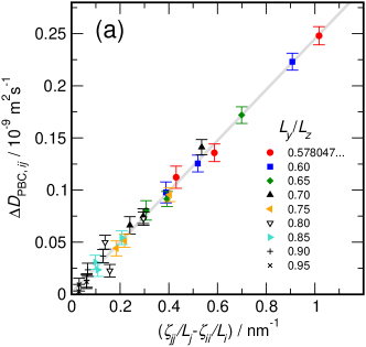
Figure 1: Analysis of the direction-dependent self-diffusion data according to Equation 4. a) Differences of the self-diffusion coefficients in $i$- and $j$-direction $\Delta D_{\mathrm{PBC},ij}\!=\!D_{\mathrm{PBC},ii}-D_{\mathrm{PBC},jj}$ with ${i,j}\in\{x,y,z\}$ vs. $\zeta_{jj}/L_{j}-\zeta_{ii}/L_{i}$ according to Equation 4 for TIP4P/2005 water at $298\,\mbox{K}$ determined from MD simulations employing orthorhombic simulation boxes with varying box-lengths ratios $L_{y}/L_{z}\!=\!L_{x}/L_{y}$. The grey solid line represent a linear fit of the data according to Equation 4, resulting in a viscosity of $\eta\!=\!(0.8957\pm 0.0178)\,\mbox{mPa}\,\mbox{s}$. b) Log-log plot of the relative error of the computed differences of the self diffusion coefficients $\hat{\sigma}(\Delta D_{\mathrm{PBC},ij})/\Delta D_{\mathrm{PBC},ij}$ given in percent, vs. $\zeta_{jj}/L_{j}-\zeta_{ii}/L_{i}$. The solid grey line represents a fitted scaling of the errors according to $(\zeta_{jj}/L_{j}-\zeta_{ii}/L_{i})^{\beta}$ with an exponent $\beta\!=\!-0.9$.

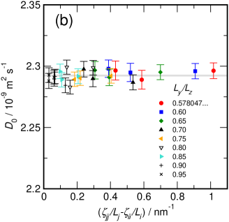
Figure 2: Shear viscositiies $\eta$ and system size independent true self-diffusion coefficients $D_{0}$ obtained for TIP4P/2005 water at $298\,\mbox{K}$, determined from MD simulations employing orthorhombic simulation boxes with varying box-lengths ratios $L_{y}/L_{z}\!=\!L_{x}/L_{y}$. a) Shear viscosities computed according to Equation 4 using self-diffusion coefficients listed in Tables 1 and 2. The grey solid line represents a viscosity of $\eta\!=\!0.8957\,\mbox{mPa}\,\mbox{s}$, representing a linear fit of the data hown in Figure 1 according to Equation 4. b) True self-diffusion coefficients $D_{0}$ obtained according to Equation 2 from data listed in Tables 1 and 2. using the average viscosity $\eta\!=\!(0.8957\pm 0.0178)\,\mbox{mPa}\,\mbox{s}$. The grey solid line represents the average value $D_{0}\!=\!2.2923\times 10^{-9}\,\mbox{m}^{2}\,\mbox{s}^{-1}$.

Self-diffusion coefficients were computed from the slope of the center-of-mass mean square displacement of the water molecules using the Einstein formula [28] according to

$$D_{\textrm{PBC}}=\frac{1}{6}\frac{\partial}{\partial t}\lim_{t\rightarrow\infty}\left<|\mathbf{r}(0)-\mathbf{r}(t)|^{2}\right>\;,$$ (12)

and

$$D_{\textrm{PBC},{ii}}=\frac{1}{2}\frac{\partial}{\partial t}\lim_{t\rightarrow\infty}\left<|r_{i}(0)-r_{i}(t)|^{2}\right>\;,$$ (13)

where $\mathbf{r}(t)=[r_{x}(t),r_{y}(t),r_{z}(t)]$ represent the position of the center of mass of a water molecule at time $t$ and the $r_{i}(t)$ are its respective components in $x$-, $y$-, and $z$-direction. All computed self-diffusion coefficients shown in Table 2 were determined from the slope of the mean square displacement of the water molecules fitted to time intervals between $15\,\mbox{ps}$ and $200\,\mbox{ps}$.

Table 2 contains direction-dependent self-diffusion coefficients $D_{\textrm{PBC},{ii}}$ obtained from MD simulations using orthorhombic unit cells with $L_{y}/L_{z}=L_{x}/L_{y}$ for various ratios $L_{y}/L_{z}$. Here a decreasing ratio $L_{y}/L_{z}$ indicates an increasing deviation from the cubic form. If the hydrodynamic interaction approach towards self-diffusion according to Equation 1 holds, we expect a linear relation between the difference between self-diffusion coefficients in different directions $i$ and $j$ with $\Delta D_{\mathrm{PBC},ij}\!=\!D_{\mathrm{PBC},ii}-D_{\mathrm{PBC},jj}$ and the difference between the Madelung constant analogue weighted with inverse box-lengths $\zeta_{jj}/L_{j}-\zeta_{ii}/L_{i}$ according to Equation 4. Figure 1a demonstrates, that this linear relationship is excellently fulfilled. A linear fit including all $9\times 3\!=\!27$ direction-dependent data points passes almost perfectly through the origin with $\Delta D_{\mathrm{PBC},ij}(0)=(0.0013\pm 0.0020)\times 10^{-9}\,\mbox{m}^{2}\,\mbox{s}^{-1}$, while the slope of the fitted solid grey line in 1a yields a viscosity of $\eta\!=\!(0.8957\pm 0.0178)\,\mbox{mPa}\,\mbox{s}$, which is consistent with the value $\eta\!=\!(0.900\pm 0.051)\,\mbox{mPa}\,\mbox{s}$ obtained for TIP4P/2005 under the same conditions (temperature and density) in Ref. [13] It is evident, however, that for near-cubic box geometries with $L_{y}/L_{z}\geq 0.95$ the error and the magnitude of $\Delta D_{\mathrm{PBC},ij}$ have almost the same size, thus rendering those systems an extremely unreliable source for determining viscosity data. This behavior is a consequence of the little variation found for the size of the computed uncertainties of the direction-dependent diffusion coefficients, as can be seen from the data shown in Table 2. This is leading to a strong increase of the relative error of $\Delta D_{\mathrm{PBC},ij}$ for $L_{y}/L_{z}\rightarrow 1$. This behavior is perfectly demonstrated in Figure 1b in the form of a log-log plot of the relative error of the computed differences of the self diffusion coefficients $\hat{\sigma}(\Delta D_{\mathrm{PBC},ij})/\Delta D_{\mathrm{PBC},ij}$ vs. $\zeta_{jj}/L_{j}-\zeta_{ii}/L_{i}$. Given the linear dependence of $\Delta D_{\mathrm{PBC},ij}$ vs. $\zeta_{jj}/L_{j}-\zeta_{ii}/L_{i}$ as shown in Figure 1a, a constant size of $\hat{\sigma}(\Delta D_{\mathrm{PBC},ij})$ would lead to an inverse proportional behavior according to

$$\frac{\hat{\sigma}(\Delta D_{\mathrm{PBC},ij})}{\Delta D_{\mathrm{PBC},ij}}\propto\left(\frac{\zeta_{jj}}{L_{j}}-\frac{\zeta_{ii}}{L_{i}}\right)^{\beta}$$ (14)

with an exponent $\beta\!=\!-1$. Due to small, albeit significant variation of $\hat{\sigma}(\Delta D_{\mathrm{PBC},ij})$ as a function of $L_{y}/L_{z}$, however, the solid grey line in Figure 1 indicates a scaling with a slightly smaller exponent $\beta\!=\!-0.9$.

According to Equation 4, we can compute an estimate of the viscosity $\eta_{ij}$ for each difference in diffusion coefficients $\Delta D_{\mathrm{PBC},ij}$. These viscosity estimates are shown in Figure 2a as a function of $\zeta_{jj}/L_{j}-\zeta_{ii}/L_{i}$. The predictive value of the most anisotropic systems is very good, the quality of the estimate, however, drops significantly for $L_{y}/L_{z}\rightarrow 1$, since $\hat{\sigma}(\eta_{ij})/\eta_{ij}\!\approx\!\hat{\sigma}(\Delta D_{\mathrm{PBC},ij})/\Delta D_{\mathrm{PBC},ij}$. In Figure 2b, the computed estimates for the true self-diffusion coefficients $D_{0}$ according to Equation 2 are shown. To compute $D_{0}$, we have used the average viscosity of $\eta\!=\!(0.8957\pm 0.0178)\,\mbox{mPa}\,\mbox{s}$. Note that Equation 2 holds up extremely well, leading to a very small statistical variation of the computed average for $D_{0}$ with no recognizable trend as a function of $L_{y}/L_{z}$, including the simulations with near-cubic box shapes. Averaging those values leads to $D_{0}=(2.2923\pm 0.0008)\times 10^{-9}\,\mbox{m}^{2}\,\mbox{s}^{-1}$. The accuracy suggested by the small statistical error, however, might be misleading, since it does not properly account for the uncertainty of the average viscosity, which would shift the whole ensemble of data points in Figure 2b simultaneously up or down.

Next, we would like to compute both $D_{0}$ and $\eta$ from the system with “magical” box length ratios of $L_{y}/L_{z}\!=\!0.57804765578$ and $L_{x}/L_{z}\!=\!0.33413909235$. Here, according to Equation 8 $D_{0}=D_{\mathrm{PBC},xx}=(2.2964\pm 0.0077)\times 10^{-9}\,\mbox{m}^{2}\,\mbox{s}^{-1}$, which is in excellent agreement with the estimate including all box shapes. The weighted average of the viscosity computed according to Equation 9 is $\eta\!=\!(0.8869\pm 0.0415)\,\mbox{mPa}\,\mbox{s}$, which is slightly smaller than the estimate from the slope of the data in Figure 1a, albeit within the range of the statistical uncertainty. Note that in Ref. [13], the estimate for $D_{0}$ and the viscosity for a system of the same number of molecules at the same density, but for a shorter simulation of just $10\,\mbox{ns}$ length (with $n_{\mathrm{W}}\!=\!20$) was obtained as $D_{0}=(2.283\pm 0.027)\times 10^{-9}\,\mbox{m}^{2}\,\mbox{s}^{-1}$ and $\eta\!=\!(0.853\pm 0.084)\,\mbox{mPa}\,\mbox{s}$. Given the 16 times longer simulation runs, we would expect a four times smaller statistical uncertainty, which coincides rather well with the computed uncertainty for $D_{0}$. The fact that the statistical uncertainty of $\eta$ is just about one-half of the value reported in Ref. [13], suggests the “magical” simulation-box procedure proposed here is less effective in estimating the viscosity than the original “OrthoBoXY”-method proposed in Ref. [13].

Note that the computed viscosities are all lying very close to the experimental value for ordinary water between $0.892\,\mbox{mPa\,s}$ and $0.893\,\mbox{mPa\,s}$ at $298.15\,\mbox{K}$, reported by Harris and Woolf [32, 33] (when using their corrected data tables listed in Ref.[33]), while the self-diffusion coefficients almost perfectly match the experimental value of Krynicki et al.[34] with $2.30\times 10^{-9}\,\text{m}^{2}\,\text{s}^{-1}$ at $298.2\,\mbox{K}$, and of Mills [35] with $2.299\times 10^{-9}\,\text{m}^{2}\,\text{s}^{-1}$ at $25^{\circ}\mbox{C}$.

Finally, it should not be left unnoticed that the data shown in Figures 1a and 2b provide excellent evidence for the validity of the hydrodynamic-interaction-based approach for correcting self-diffusion coefficients for non-cubic geometries.

V Conclusion

We have derived equations representing a generalized “OrthoBoXY” procedure, which can be applied to MD simulations of any orthorhombic box geometry for determining both the system size independent true self-diffusion coefficient $D_{0}$ and the shear viscosity $\eta$. We have tested this approach by using NVT MD simulations of systems containing 1536 TIP4P/2005 water molecules at a density of $\rho\!=\!0.9972\,\text{g}\,\text{cm}^{-3}$ and a temperature of $T\!=\!298\,\mbox{K}$ using varying box geometries. These systems obey the condition $L_{y}/L_{z}\!=\!L_{x}/L_{y}$, while the ratio $L_{y}/L_{z}$ was systematically varied. In particular, we have explored the feasibility of employing box shapes more akin to the cubic form.

We have demonstrated, that we are indeed able to determine the true self-diffusion coefficient $D_{0}$ for TIP4P/2005 water without prior knowledge of the shear viscosity from single MD simulation runs using this generalized approach, similar to what we have achieved in our previous paper using simulation boxes with $L_{z}/L_{x}\!=\!L_{z}/L_{y}\!=\!2.7933596497$.[13] The computed values for $D_{0}$ agree well with the values determined from MD simulations employing both orthorhombic and cubic unit cells discussed in Ref.[13]. Moreover, both the computed self-diffusion coefficient and shear viscosity agree nearly quantitatively with the experimentally observed data for water at $298\,\mbox{K}$.

However, the idea, to use box shapes more akin to the cubic form turns out to be only partially practical, since the small differences in direction-dependent self-diffusion coefficients observed for near-cubic geometries lead to unsustainably large relative uncertainties for the computed viscosities. Large differences between box-length, are instead the preferred choice. This leads us to the conclusion, that the original “OrthoBoXY”-approach outlined in Ref.[13] has to be considered already quite efficient.

Instead, another “magical” set of box-length ratios has been discovered with $L_{y}/L_{z}\!=\!0.57804765578$ and $L_{x}/L_{z}\!=\!0.33413909235$, where the self-diffusion coefficient in $x$-direction becomes system sized independent, such that $D_{0}\!=\!D_{\mathrm{PBC,}xx}$. An expression for determining the viscosity $\eta$, employing $D_{\mathrm{PBC,}yy}$ and $D_{\mathrm{PBC,}zz}$, is given by Equation 9. However, from the standpoint of box anisotropy, this box shape is deemed less preferable to the original “OrthoBoXY”-approach, since the smallest box-length is about $20$ per cent smaller than the smallest box length of a system of the same size using the original “OrthoBoXY”-approach under the same conditions. Moreover, the simulations indicate, that also uncertainty of the predicted viscosity is slightly worse than that of the original “OrthoBoXY”-procedure.

Data Availability Statement

The codes of GROMACS and MOSCITO are freely available. Input parameter and topology files for the MD simulations and the code for computing the Madelung constant analogues for cubic and orthorhombic lattices can be downloaded from GitHub via https://github.com/Paschek-Lab/OrthoBoXY/

References

- [1] R. Taylor and R. Krishna. Multicomponent Mass Transfer. John Wiley & Sons Inc., New York, 1993.
- [2] C. L. Yaws. Handbook of Viscosity. Gulf Professional Publishing, Houston, Texas, 1st edition, 1994.
- [3] E. J. Maginn, R. A. Messerly, D. J. Carlson, D. R. Roe, and J. R. Elliot. Best practices for computing transport properties 1.self-diffusivity and viscosity from equilibrium molecular dynamics [articlev1.0]. Living. Comp. Mol. Sci., 1:6324, 2020.
- [4] Krishna R. Describing the diffusion of guest molecules inside porous structures. J. Phys. Chem. C, 113:19756–19781, 2009.
- [5] W.-J. Li, Z. Li, Z. Ma, P. Zhang, Y. Lu, C. Wang, Q. Jia, X.-B. Cheng, and H.-D. Hu. Ab initio determination on diffusion coefficient and viscosity of FeNi fluid under earth’s core condition. Sci. Rep., 12:21255, 2022.
- [6] A. T. Celebi, S. H. Jamali, A. Bardow, T. J. H. Vlugt, and O. A. Moultos. Finite-size effects of diffusion coefficients computed from molecular dynamics: a review of what we have learned so far. Mol. Simul., 47:831–845, 2021.
- [7] M. Erdös, M. Frangou, T. J. H. Vlugt, and O. A. Moultos. Diffusivity of -, -, -cyclodextrin and the inclusion complex of -cyclodextrin: Ibuprofen in aqueous solutions; a molecular dynamics simulation study. Fluid Ph. Equilib., 528:112842, 2020.
- [8] B. Dünweg and K. Kremer. Molecular dynamics simulation of a polymer chain in solution. J. Chem. Phys., 99:6983–6997, 1993.
- [9] I.-C. Yeh and G. Hummer. System-size dependence of diffusion coefficients and viscosities from molecular dynamics simulations with periodic boundary conditions. J. Phys. Chem. B, 108:15873–15879, 2004.
- [10] G. Kikugawa, T. Nakano, and T. Ohara. Hydrodynamic consideration of the finite size effect on the self-diffusion coefficient in a periodic rectangular parallelepiped system. J. Chem. Phys., 143:024507, 2015.
- [11] M. Vögele and G. Hummer. Divergent diffusion coefficients in simulations of fluids and lipid membranes. J. Phys. Chem. B, 120:8722–8732, 2016.
- [12] O. A. Moultos, Y. Zhang, I. O. Tsimpanogiannis, I. G. Economou, and E. J. Maginn. System-size corrections for self-diffusion coefficients calculated from molecular dynamics simulations: The case of CO2, n-alkanes, and poly(ethylene glycol) dimethyl ethers. J. Chem. Phys., 145:074109, 2016.
- [13] J. Busch and D. Paschek. OrthoBoXY: A simple way to compute true self-diffusion coefficients from MD simulations with periodic boundary conditions without prior knowledge of the viscosity. J. Phys. Chem. B, 127:7983–7987, 2023.
- [14] G. Kikugawa, S. Ando, J. Suzuki, Y. Naruke, T. Nakano, and T. Ohara. Effect of the computational domain size and shape on the self-diffusion coefficient in a Lennard-Jones liquid. J. Chem. Phys., 142:024503, 2015.
- [15] J. G. Kirkwood and J. Riseman. The intrinsic viscosities and diffusion constants of flexible macromolecules in solution. J. Chem. Phys., 16:565–573, 1948.
- [16] H. Hasimoto. On the periodic fundamental solutions of the stokes equations and their application to viscous flow past a cubic array of spheres. J. Fluid Mech., 5:317–328, 1959.
- [17] C. W. J. Beenakker. Ewald sum of the Rotne-Prager tensor. J. Chem. Phys., 85:1581–1582, 1986.
- [18] J. L. F. Abascal and C. Vega. A general purpose model for the condensed phases of water: TIP4P/2005. J. Chem. Phys., 123:234505, 2005.
- [19] C. Vega and J. L. F. Abascal. Simulating water with rigid non-polarizable models: a general perspective. Phys. Chem. Chem. Phys., 13:19663–19688, 2011.
- [20] D. van der Spoel, E. Lindahl, B. Hess, G. Groenhof, A. E. Mark, and H. J. C. Berendsen. GROMACS: fast, flexible, and free. J. Comput. Chem., 26(16):1701–1718, 2005.
- [21] B. Hess, C. Kutzner, D. van der Spoel, and E. Lindahl. Gromacs 4: algorithms for highly efficient, load-balanced, and scalable molecular simulation. J. Chem. Theory Comput., 4(3):435–447, 2008.
- [22] S.Nosé. A molecular dynamics method for simulations in the canonical ensemble. Mol. Phys., 52:255–268, 1984.
- [23] W. G. Hoover. Canonical dynamics: Equilibrium phase-space distributions. Phys. Rev. A, 31:1695–1697, 1985.
- [24] U. Essmann, L. Petera, M. Berkowitz, T. Darden, H. Lee, and L. Pedersen. A smooth particle mesh Ewald method. J. Chem. Phys., 103:8577–8593, 1995.
- [25] C. L. Wennberg, T. Murtola, B. Hess, and E. Lindahl. Lennard-Jones lattice summation in bilayer simulations has critical effects on surface tension and lipid properties. J. Chem. Theory Comput., 9:3527–3537, 2013.
- [26] C. L. Wennberg, T. Murtola, S. Páll, M. J. Abraham, B. Hess, and E. Lindahl. Direct-space corrections enable fast and accurate Lorentz-Berthelot combination rule Lennard-Jones lattice summation. J. Chem. Theory Comput., 11:5737–5746, 2015.
- [27] S. Miyamoto and P. A. Kollman. Settle: An analytical version of the SHAKE and RATTLE algorithm for rigid water models. J. Comput. Chem., 13:952–962, 1992.
- [28] M. P. Allen and D. J. Tildesley. Computer Simulation of Liquids. Oxford University Press, Clarendon, Oxford, 1987.
- [29] W. H. Press, S. A. Teukolsky, W. T. Vetterling, and P. Flannery. Numerical Recipes in C: The Art of Scientific Computing. Cambridge University Press, Cambridge, MA, 2 edition, 1992.
- [30] https://github.com/Paschek-Lab/OrthoBoXY.
- [31] GROMACS development team. GROMACS Documentation 2023.2, 2023. https://doi.org/10.5281/zenodo.8134388.
- [32] K. R. Harris and L. A. Woolf. Temperature and volume dependence of the viscosity of water and heavy water at low temperatures. J. Chem. Eng. Data, 49:1064–1069, 2004.
- [33] K. R. Harris and L. A. Woolf. Correction: Temperature and volume dependence of the viscosity of water and heavy water at low temperatures. J. Chem. Eng. Data, 49:1851, 2004.
- [34] K. Krynicki, C. D. Green, and D. W. Sawyer. Pressure and temperature dependence of self-diffusion in water. Faraday Discuss. Chem. Soc., 66:199–208, 1978.
- [35] R. Mills. Self-diffusion in normal and heavy water in the range 1-45∘. J. Phys. Chem., 77:685–688, 1973.