Efficient Algorithms for the CCA Family: Unconstrained Losses with Unbiased Gradients

Abstract

The Canonical Correlation Analysis (CCA) family of methods is foundational in multi-view learning. Regularised linear CCA methods can be seen to generalise Partial Least Squares (PLS) and be unified with a Generalized Eigenvalue Problem (GEP) framework. However, classical algorithms for these linear methods are computationally infeasible for large-scale data. Extensions to Deep CCA show great promise, but current training procedures are slow and complicated. First we propose a novel unconstrained objective that characterizes the top subspace of GEPs. Our core contribution is a family of fast algorithms for stochastic PLS, stochastic CCA, and Deep CCA, simply obtained by applying stochastic gradient descent (SGD) to the corresponding CCA objectives. These methods show far faster convergence and recover higher correlations than the previous state-of-the-art on all standard CCA and Deep CCA benchmarks. This speed allows us to perform a first-of-its-kind PLS analysis of an extremely large biomedical dataset from the UK Biobank, with over 33,000 individuals and 500,000 variants. Finally, we not only match the performance of ‘CCA-family’ Self-Supervised Learning (SSL) methods on CIFAR-10 and CIFAR-100 with minimal hyper-parameter tuning, but also establish the first solid theoretical links to classical CCA, laying the groundwork for future insights.

1 Introduction

CCA methods learn highly correlated representations of multi-view data. The original CCA method of Hotelling (1933) learns low-dimensional representations from linear transformations. Notable extensions to ridge-regularized CCA (Vinod, 1976), Partial Least Squares (PLS), and multi-view CCA (Wong et al., 2021) allow one to use CCA in high dimensional regimes, and with three or more views of data. More recently, a variety of Deep CCA methods (Andrew et al., 2013) have been proposed which learn representations obtained from non-linear transformations of the data, parameterized by deep neural networks; Deep CCA has seen excellent empirical results, and is so foundational for deep multi-view learning that it secured a runner-up position for the test-of-time award at ICML 2023 (ICML, 2023).

However, there are significant computational challenges when applying these CCA methods to large scale data. Classical algorithms for linear CCA methods require computing full covariance matrices and so scale quadratically with dimension, becoming intractable for many large-scale datasets of practical interest. There is therefore great interest in approximating solutions for CCA in stochastic or data-streaming settings (Arora et al., 2012). Large scale data also challenges existing full-batch algorithms for Deep CCA, and their stochastic counterparts are not only complex to implement but also difficult to train (Wang et al., 2015b).

Self-supervised learning (SSL) methods are now state of the art in image classification. They also learn useful representations of data, usually from pretext tasks or objectives that exploit some inherent structure or property of the data. Remarkably, SSL methods can even perform zero-shot classification: where the representations are learnt without any explicit labels or supervision (Balestriero et al., 2023). Of particular interest to us is the so-called CCA family of SSL methods. Like CCA, these aim to transform a pair of views of data to a pair of similar representations. It is known that a number of algorithms in this class are closely related to CCA (Balestriero & LeCun, 2022), notably including Barlow Twins (Zbontar et al., 2021) and VICReg (Bardes et al., 2021). However, the specific details of this relationship are poorly understood.

In section 2 we provide a unified approach to all the CCA methods introduced above, emphasizing objectives which are functions of the joint distributions of the transformed variables. Versions of all the linear CCA methods can be defined by solutions to certain Generalized Eigenvalue Problems (GEPs); this provides a particularly convenient way to relate a large number of equivalent objectives.

Section 3 outlines our core conceptual contributions. Firstly, with proposition 3.1 we present an unconstrained loss function that characterizes solutions to GEPs; this is based on the Eckhart–Young inequality and has appealing geometrical properties. We apply this to the GEP formulation of CCA and construct unbiased estimates of the loss and its gradients from mini-batches of data. These loss functions can therefore be optimized out-of-the-box using standard frameworks for deep learning. This immediately gives a unified family of algorithms for CCA, Deep CCA, and indeed SSL.

Our CCA algorithms dominate existing state-of-the-art methods across a wide range of benchmarks, presented in section 5. For stochastic CCA, our method not only converges faster but also achieves higher correlation scores than existing techniques. For Deep CCA and Deep Multiview CCA our unbiased stochastic gradients yield significantly better validation correlations and allow the use of smaller mini-batches in memory constrained applications. We also demonstrate how useful our algorithms are in practice with an pioneering real-world case study. We apply stochastic Partial Least Squares (PLS) to an extremely high-dimensional dataset from the UK Biobank dataset – all executed on a standard laptop. Our algorithm opens the door to problems previously deemed intractable in biomedical data analytics. Finally, our SSL method achieves comparable performance to VICReg and Barlow Twins, despite having no hyperparameters in the objective. This frees computational resources to tune more critical hyperparameters, such as architecture, optimizer or augmentations. In addition, our method appears more robust to these other hyperparameters, has a clear theoretical foundation, and naturally generalizes to the multi-view setting. Furthermore, we also provide the first rigorous results relating VICReg and Barlow Twins to CCA, opening up avenues to better theoretical understanding.

2 A unified approach to the CCA family

Suppose we have a sequence of vector-valued random variables $X^{(i)}\in\mathbb{R}^{D^{(i)}}$ for $i\in\{1,\dots,I\}$. We want to learn meaningful $K$-dimensional representations

$$Z^{(i)}=f^{(i)}(X^{(i)};\theta^{(i)}).$$ (1)

For convenience, define $D=\sum_{i=1}^{I}D^{(i)}$ and $\theta=\left(\theta^{(i)}\right)_{i=1}^{I}$. We will consistently use the superscripts $i,j\in[I]$ for views and subscripts $l,k\in[K]$ for dimensions of representations - i.e. to subscript dimensions of $Z^{(i)},f^{(i)}$. Later on we will introduce total number of samples $N$ and mini-batch size $M$.

2.1 Background: GEPs in linear algebra

A Generalized Eigenvalue Problem (GEP) is defined by two symmetric matrices $A,B\in\mathbb{R}^{D\times D}$ (Stewart & Sun, 1990). They are usually characterized by the set of solutions to the equation:

$$Au=\lambda Bu$$ (2)

with $\lambda\in\mathbb{R},u\in\mathbb{R}^{D}$, called (generalized) eigenvalue and (generalized) eigenvector respectively. We shall only consider the case where $B$ is positive definite to avoid degeneracy. Then the GEP becomes equivalent to an eigen-decomposition of the symmetric matrix $B^{\shortminus\nicefrac{{1}}{{2}}}AB^{\shortminus\nicefrac{{1}}{{2}}}$. This is key to the proof of our new characterization. In addition, one can find a basis of eigenvectors spanning $\mathbb{R}^{D}$. We define a top-$K$ subspace to be one spanned by some set of eigenvectors $u_{1},\dots,u_{K}$ with the top-$K$ associated eigenvalues $\lambda_{1}\geq\dots\geq\lambda_{K}$. We say a matrix $U\in\mathbb{R}^{D\times K}$ defines a top-$K$ subspace if its columns span one.

2.2 The CCA Family

The classical notion CCA (Hotelling, 1992) considers two views, $I=2$, and constrains the representations to be linear transformations

$$Z^{(i)}_{k}=\langle u_{k}^{(i)},X^{(i)}\rangle.$$ (3)

The objective is to find the weights or canonical directions $u_{k}^{(i)}$ which maximize the canonical correlations $\rho_{k}=\operatorname{Corr}(Z^{(1)}_{k},Z^{(2)}_{k})$ sequentially, subject to orthogonality with the previous pairs of the transformed variables. It is well known that CCA is equivalent to a singular value decomposition (SVD) of the matrix $\mathrm{Var}(X^{(1)})^{\shortminus\nicefrac{{1}}{{2}}}\mathrm{Cov}(X^{(1)},X^{(2)})\mathrm{Var}(X^{(2)})^{\shortminus\nicefrac{{1}}{{2}}}$. It is slightly less well known (Borga, 1998) that this is equivalent to a GEP where:

$$A=\begin{pmatrix}0&\mathrm{Cov}(X^{(1)},X^{(2)})\\ \mathrm{Cov}(X^{(2)},X^{(1)})&0\end{pmatrix},\quad B=\begin{pmatrix}\mathrm{Var}(X^{(1)})&0\\ 0&\mathrm{Var}(X^{(2)})\end{pmatrix},\quad u=\begin{pmatrix}u^{(1)}\\ u^{(2)}\end{pmatrix}.$$ (4)

CCA therefore has notions of uniqueness similar to those for SVD or GEPs: the weights are not in general unique, but the canonical correlations $1\geq\rho_{1}\geq\rho_{2}\geq\dots\geq 0$ are unique (Mills-Curran, 1988). Therefore, we can write:

$$\operatorname{CCA}_{K}(X^{(1)},X^{(2)})\vcentcolon=(\rho_{k})_{k=1}^{K}$$ (5)

Sample CCA: in practice we do not have access to the population distribution but to a finite number of samples; the classical estimator is defined by replacing the population covariances in eq. 59 with sample covariances. Unfortunately, this estimator breaks down when $N\leq\max(D^{(1)},D^{(2)})$; giving arbitrary correlations of 1 and meaningless directions.

Ridge-regularized CCA: the most straightforward way to prevent this overfitting is to add a ridge regularizer (Vinod, 1976). Taking maximal ridge regularization recovers Partial Least Squares PLS (Mihalik et al., 2022), a widely used technique for multi-view learning. Even these simple modifications to CCA can be very effective at preventing overfitting in high dimensions (Mihalik et al., 2022).

Multi-view CCA (MCCA): extends two-view CCA to deal with three or more views of data. Unfortunately, many of the different equivalent formulations of two-view CCA are no longer equivalent in the multi-view setting, so there are many different extensions to choose from; see section 4. Of most interest to us is the formulation of Nielsen (2002); Wong et al. (2021) that extends the GEP formulation of eq. 59, which we next make precise and will simply refer to as MCCA from now.

Unified GEP formulation: this GEP formulation of MCCA can be presented in a unified framework generalizing CCA and ridge-regularized extensions. Indeed, we now take $A,B_{\alpha}\in\mathbb{R}^{D\times D}$ to be block matrices $A=(A^{(ij)})_{i,j=1}^{I},B_{\alpha}=(B_{\alpha}^{(ij)})_{i,j=1}^{I}$ where the diagonal blocks of $A$ are zero, the off-diagonal blocks of $B_{\alpha}$ are zero, and the remaining blocks are defined by:

$$A^{(ij)} =\mathrm{Cov}(X^{(i)},X^{(j)})\text{ for }i\neq j,\quad B_{\alpha}^{(ii)}=\alpha_{i}I_{D^{(i)}}+(1-\alpha_{i})\mathrm{Var}(X^{(i)})$$ (6)

Where $\alpha\in[0,1]^{I}$ is a vector of ridge penalty parameters: taking $\alpha_{i}=0\>\forall i$ recovers CCA and $\alpha=1\>\forall i$ recovers PLS. We may omit the subscript $\alpha$ when $\alpha=0$ and we recover the ‘pure CCA’ setting; in this case, following eq. 5 we can define $\operatorname{MCCA}_{K}(X^{(1)},\dots,X^{(I)})$ to be the vector of the top-$K$ generalized eigenvalues.

Deep CCA: was originally introduced in Andrew et al. (2013); this was extended to an GEP-based formulation of Deep Multi-view CCA (DMCCA) in Somandepalli et al. (2019). This can be defined using our $\operatorname{MCCA}$ notation as maximizing

$$\lVert\operatorname{MCCA}_{K}\left(Z^{(1)},...Z^{(I)}\right)\rVert_{2}$$ (7)

over parameters $\theta$ of neural networks defining the representations $Z^{(i)}=f^{(i)}(X^{(i)};\theta^{(i)})$ for $i\in[I]$.

3 Novel Objectives and Algorithms

3.1 Unconstrained objective for GEPs

First, we present proposition 3.1, a formulation of the top-$K$ subspace of GEP problems, which follows by applying the Eckhart–Young–Minsky inequality (Stewart & Sun, 1990) to the eigen-decomposition of $B^{\shortminus\nicefrac{{1}}{{2}}}AB^{\shortminus\nicefrac{{1}}{{2}}}$. However, making this rigorous requires some technical care which we defer to the proof in supplement A.

Proposition 3.1 (Eckhart–Young inspired objective for GEPs).

The top-$K$ subspace of the GEP $(A,B)$ can be characterized by minimizing the following objective over $U\in\mathbb{R}^{D\times K}$:

$$\mathcal{L}_{\text{EY-GEP}}(U)\vcentcolon=\operatorname{trace}\left(-2\,U^{T}AU+\left(U^{T}BU\right)\left(U^{T}BU\right)\right)$$ (8)

Moreover, the minimum value is precisely $-\sum_{k=1}^{K}\lambda_{k}^{2}$, where $(\lambda_{k})$ are the generalized eigenvalues.

This objective also has appealing geometrical properties. It is closely related to a wide class of unconstrained objectives for PCA and matrix completion which have no spurious local optima (Ge et al., 2017), i.e. all local optima are in fact global optima. This implies that certain local search algorithms, such as stochastic gradient descent, should indeed converge to a global optimum.

Proposition 3.2.

[No spurious local minima] The objective $\mathcal{L}_{\text{EY-GEP}}$ has no spurious local minima. That is, any matrix $\bar{U}$ that is a local minimum of $\mathcal{L}_{\text{EY-GEP}}$ must in fact be a global minimum.

It is also possible to make this argument quantitative by proving a version of the strict saddle property from Ge et al. (2017; 2015); we state an informal version here and give full details in appendix B.

Corollary 3.1 (Informal: Polynomial-time Optimization).

Under certain conditions on the eigenvalues and generalized eigenvalues of $(A,B)$, one can make quantitative the claim that: any $U_{K}\in\mathbb{R}^{D\times K}$ is either close to a global optimum, has a large gradient $\nabla\mathcal{L}_{\text{EY-GEP}}$, or has Hessian $\nabla^{2}\mathcal{L}_{\text{EY-GEP}}$ with a large negative eigenvalue.

Therefore, for appropriate step-size sequences, certain local search algorithms, such as sufficiently noisy SGD, will converge in polynomial time with high probability.

3.2 Corresponding Objectives for the CCA family

For the case of linear CCA we have $U^{T}AU=\sum_{i\neq j}\mathrm{Cov}(Z^{(i)},Z^{(j)}),U^{T}BU=\sum_{i}\mathrm{Var}(Z^{(i)})$. To help us extend this to the general case of nonlinear transformations, eq. 1, we define the analogous matrices of total between-view covariance and total within-view variance

$$\vphantom{\bigl{(}\bigr{)}}C(\theta)=\sum_{i\neq j}\mathrm{Cov}(Z^{(i)},Z^{(j)}),\quad V(\theta)=\sum_{i}\mathrm{Var}(Z^{(i)})$$ (9)

In the case of linear transformations, eq. 3, it makes sense to add a ridge penalty so we can define

$$V_{\alpha}(\theta)=\sum_{i}\alpha_{i}{U^{(i)\,T}}U^{(i)}+(1-\alpha_{i})\mathrm{Var}(Z^{(i)})$$ (10)

This immediately leads to following unconstrained objective for the CCA-family of problems.

Definition 3.1 (Family of EY Objectives).

Learn representations $Z^{(i)}=f^{(i)}(X^{(i)};\theta^{(i)})$ minimizing

$$\mathcal{L}_{\text{EY}}(\theta)=-2\operatorname{trace}C(\theta)+\lVert V_{\alpha}(\theta)\rVert_{F}^{2}$$ (11)

Unbiased estimates: since empirical covariance matrices are unbiased, we can construct unbiased estimates to $C,V$ from a batch of transformed variables $\mathbf{Z}$.

$$\hat{C}(\theta)[\mathbf{Z}]=\sum_{i\neq j}\widehat{\mathrm{Cov}}(\mathbf{Z}^{(i)},\mathbf{Z}^{(j)}),\quad\hat{V}(\theta)[\mathbf{Z}]=\sum_{i}\widehat{\mathrm{Var}}(\mathbf{Z}^{(i)})$$ (12)

In the linear case we can construct $\hat{V}_{\alpha}(\theta)[\mathbf{Z}]$ analogously by plugging sample covariances into eq. 10. Then if $\mathbf{Z},\mathbf{Z}^{\prime}$ are two independent batches of transformed variables, the batch loss

$$\hat{\mathcal{L}}_{\text{EY}}[\mathbf{Z},\mathbf{Z}^{\prime}]\vcentcolon=-2\operatorname{trace}\hat{C}[\mathbf{Z}]+\langle\hat{V}_{\alpha}[\mathbf{Z}],\hat{V}_{\alpha}[\mathbf{Z}^{\prime}]\rangle_{F}$$ (13)

gives an unbiased estimate of $\mathcal{L}_{\text{EY}}(\theta)$.This loss is a differentiable function of $\mathbf{Z},\mathbf{Z}^{\prime}$ and so also of $\theta$.

Simple algorithms: We first define a very general algorithm using these estimates in Algorithm 1. In the next section we apply this algorithm to multi-view stochastic CCA and PLS, and Deep CCA.

  Input: data stream of mini-batches $(\mathbf{X}(b))_{b=1}^{\infty}$ where each consists of $M$ samples from the original dataset. Learning rate $(\eta_{t})_{t}$. Number of time steps $T$. Class of functions $f(\cdot;\theta)$ whose outputs are differentiable with respect to $\theta$.

  Initialize: $\hat{\theta}$ with suitably random entries

  for $t=1$ to $T$ do

     Obtain two independent mini-batches $\mathbf{X}(b),\mathbf{X}(b^{\prime})$ by sampling $b,b^{\prime}$ independently

     Compute batches of transformed variables $\mathbf{Z}(b)=f(\mathbf{X}(b);\theta),\mathbf{Z}(b^{\prime})=f(\mathbf{X}(b^{\prime});\theta)$

     Estimate loss $\hat{\mathcal{L}}_{\text{EY}}(\theta)$ using eq. 13

     Obtain gradients by back-propagation and step with your favourite optimizer.

  end for

Algorithm 1 GEP-EY: General algorithm for learning correlated representations

3.3 Applications to (multi-view) stochastic CCA and PLS, and Deep CCA

Lemma 3.1 (Objective recovers GEP formulation of linear (multi-view) CCA).

When the $f^{(i)}$ are linear, as in eq. 3, the population loss from eq. 11 recovers MCCA as defined in section 2.2.

Proof.

By construction, for linear MCCA we have $C=U^{T}AU,\,V_{\alpha}=U^{T}B_{\alpha}U$, where $(A,B_{\alpha})$ define the GEP for MCCA introduced in eq. 6. So $\mathcal{L}_{\text{EY}}(U)=\mathcal{L}_{\text{EY-GEP}}(U)$ and by proposition 3.1 the optimal set of weights define a top-$K$ subspace of the GEP, and so is a MCCA solution. ∎

Moreover, by following through the chain of back-propagation, we obtain gradient estimates in $\mathcal{O}(MKD)$ time. Indeed, we can obtain gradients for the transformed variables in $\mathcal{O}(MK^{2})$ time so the dominant cost is then updating $U$; we flesh this out with full details in appendix E.

Lemma 3.2.

[Objective recovers Deep Multi-view CCA] Assume that there is a final linear layer in each neural network $f^{(i)}$. Then at any local optimum, $\hat{\theta}$, of the population problem, we have

$$\mathcal{L}_{\text{EY}}(\hat{\theta})=-\lVert\operatorname{MCCA}_{K}(\hat{Z})\rVert_{2}^{2}$$

where $\hat{Z}=f_{\hat{\theta}}(X)$. Therefore, $\hat{\theta}$ is also a local optimum of objectives from Andrew et al. (2013); Somandepalli et al. (2019) as defined in eq. 7.

Proof sketch: see section C.1 for full details..

Consider treating the penultimate-layer representations as fixed, and optimising over the weights in the final layer. This is precisely equivalent to optimising the Eckhart-Young loss for linear CCA where the input variables are the penultimate-layer representations. So by proposition 3.2, a local optimum is also a global optimum, and by proposition 3.1 the optimal value is the negative sum of squared generalised eigenvalues. ∎

3.4 Application to SSL

We can directly apply Algorithm 1 to SSL. If we wish to have the same neural network transforming each view, we can simply tie the weights $\theta^{(1)}=\theta^{(2)}$. When the paired data are generated from applying independent, identically distributed (i.i.d.) augmentations to the same original datum, it is intuitive that tying the weights is a sensible procedure, and perhaps acts as a regulariser. We make certain notions of this intuition precise for CCA and Deep CCA in appendix C.

To provide context for this proposal, we also explored in detail how VICReg and Barlow twins are related to CCA. For now we focus on VICReg, whose loss can be written as

$$\mathcal{L}_{\text{VR}}(Z^{(1)},Z^{(2)}) =\gamma\mathbb{E}\lVert Z^{(1)}-Z^{(2)}\rVert^{2}+\sum_{i\in\{1,2\}}\bigg{[}\alpha\sum_{k=1}^{K}\left(1\shortminus\sqrt{\mathrm{Var}(Z^{(i)}_{i})}\right)_{+}+\beta\sum_{\begin{subarray}{c}k,l=1\\ k\neq l\end{subarray}}^{K}\mathrm{Cov}(Z^{(i)}_{k},Z^{(i)}_{l})^{2}\bigg{]}$$

where $\alpha,\beta,\gamma>0$ are tuning parameters and, as in the framework of section 2, the $Z^{(1)},Z^{(2)}$ are $K$-dimensional representations, parameterised by neural networks in eq. 1. Our main conclusions regarding optima of the population loss are:

• Consider the linear setting with untied weights. Then global optimisers of the VICReg loss define CCA subspaces, but may not be of full rank.

• Consider the linear setting with tied weights and additionally assume that the data are generated by i.i.d. augmentations. Then the same conclusion holds.

• In either of these settings, the optimal VICReg loss is a component-wise decreasing function of $\operatorname{CCA}_{K}(X^{(1)},X^{(2)})$ the vector of population canonical correlations.

• VICReg can therefore be interpreted as a formulation of Deep CCA, but one that will not in general recover full rank representations.

We give full mathematical details and further discussion in appendix D. The analysis for Barlow twins is more difficult, but we present a combination of mathematical and empirical arguments which suggest all the same conclusions hold, again see appendix D.

4 Related Work

Stochastic PLS and CCA: To the best of our knowledge, the state-of-the-art in Stochastic PLS and CCA are the subspace Generalized Hebbian Algorithm (SGHA) of Chen et al. (2019) and $\gamma$-EigenGame from Gemp et al. (2020; 2021). Specifically, SGHA utilizes a Lagrange multiplier heuristic along with saddle-point analysis, albeit with limited convergence guarantees. EigenGame focuses on top-k subspace learning but introduces an adaptive whitening matrix in the stochastic setting with an additional hyperparameter. Both methods set the benchmarks we aim to compare against in the subsequent experimental section. Like our method, both can tackle other symmetric Generalized Eigenvalue Problems in principle.

DCCA and Deep Multiview CCA: The deep canonical correlation analysis (DCCA) landscape comprises three principal approaches with inherent limitations. The first, known as the full-batch approach, uses analytic gradient derivations based on the full sample covariance matrix (Andrew et al., 2013). The second involves applying the full batch objective to large mini-batches, an approach referred to as DCCA-STOL (Wang et al., 2015a). However, this approach gives biased gradients and therefore requires batch sizes much larger than the representation size in practice. This is the approach taken by both DMCCA (Somandepalli et al., 2019) and DGCCA (Benton et al., 2017) . The final set of approaches use an adaptive whitening matrix (Wang et al., 2015b; Chang et al., 2018) to mitigate the bias of the Deep CCA objective. However, the authors of DCCA-NOI highlight that the associated time constant complicates analysis and requires extensive tuning. These limitations make existing DCCA methods less practical and resource-efficient.

Self-Supervised Learning: Barlow Twins and VICReg have come to be known as part of the canonical correlation family of algorithms (Balestriero et al., 2023). Barlow Twins employs a redundancy reduction objective to make the representations of two augmented views both similar and decorrelated (Zbontar et al., 2021). Similarly, VICReg uses variance-invariance-covariance regularization, which draws upon canonical correlation principles, to achieve robust performance in diverse tasks (Bardes et al., 2021). These methods serve as vital baselines for our experiments, owing to their foundational use of canonical correlation ideas.

5 Experiments

5.1 Stochastic CCA

First, we compare our proposed method, CCA-EY, to the baselines of $\gamma$-EigenGame and SGHA. Our experimental setup is almost identical to that of Meng et al. (2021); Gemp et al. (2022); unlike Gemp et al. (2022) we do not simplify the problem by first performing PCA on the data before applying the CCA methods, which explains the decrease in performance of $\gamma$-EigenGame compared to their original work. All models are trained for a single epoch with varying mini-batch sizes ranging from 5 to 100. We use Proportion of Correlation Captured (PCC) as our evaluation metric, defined as $\text{PCC}=(\sum_{i=k}^{K}\rho_{k})/({\sum_{k=1}^{K}\rho_{k}^{*}})$ where $\rho_{k}$ are the full batch correlations of the learnt representations, and $\rho_{k}^{*}$ are the canonical correlations computed numerically from the full batch covariance matrices.

Observations: Figure 1 compares the algorithms on the MediaMill dataset. fig. 1(a) shows that CCA-EY consistently outperforms both $\gamma$-EigenGame and SGHA in terms of PCC across all evaluated mini-batch sizes. fig. 1(b) examines the learning curves for batch sizes 5 and 100 in more detail; CCA-EY appears to learn more slowly than SGHA at the start of the epoch, but clearly outperforms SGHA as the number of samples seen increases. $\gamma$-EigenGame significantly underperforms SGHA and CCA-EY, particularly for small batch sizes.

Further experiments: we conduct analogous experiments on the Split CIFAR dataset in supplementary material F and observe identical behaviour.

(a)

(b)

Figure 1: Stochastic CCA on MediaMill using the Proportion of Correlation Captured (PCC) metric: (a) Across varying mini-batch sizes, trained for a single epoch, and (b) Training progress over a single epoch for mini-batch sizes 5, 100. Shaded regions signify $\pm$ one standard deviation around the mean of 5 runs.

5.2 Deep CCA

Second, we compare DCCA-EY against the DCCA methods described in section 4. The experimental setup is identical to that of Wang et al. (2015b). We learn $K=50$ dimensional representations, using mini-batch sizes ranging from 20 to 100 and train for 50 epochs. Because there is no longer a ground truth we have to use Total Correlation Captured (TCC), given by $\text{TCC}=\sum_{i=k}^{K}\rho_{k}$ where $\rho_{k}$ are now the empirical correlations between the representations on a validation set.

Observations: Figure 2 compares the methods on the splitMNIST dataset. DCCA-STOL captures significantly less correlation than the other methods, and breaks down when the mini-batch size is less than the dimension $K=50$ due to low rank empirical covariances. DCCA-NOI performs similarly to DCCA-EY but requires careful tuning of an additional hyperparameter, and shows significantly slower speed to convergence (Figure 2(b)).

Further experiments: we conduct analogous experiments on the XRMB dataset in supplementary material G and observe identical behaviour.

(a)

(b)

Figure 2: Deep CCA on SplitMNIST using the Validation TCC metric: (a) after training each model for 50 epochs with varying batch sizes; (b) learning progress over 50 epochs.

5.3 Deep Multiview CCA: Robustness Across Different Batch Sizes

Third, we compare DCCA-EY to the existing DMCCA and DGCCA methods on the mfeat dataset; this contains 2,000 handwritten numeral patterns across six distinct feature sets, including Fourier coefficients, profile correlations, Karhunen-Love coefficients, pixel averages in $2\times 3$ windows, Zernike moments, and morphological features. We again learn $K=50$ dimensional representations, but now train for 100 epochs. We use a multiview extension of the TCC metric, which averages correlation across views; we call this Total Multiview Correlation Captured (TMCC), defined as $\text{TMCC}=\sum_{k=1}^{K}\frac{1}{I(I-1)}\sum_{i,j\leq I,i\neq j}\text{corr}(Z_{k}^{(i)},Z_{k}^{(j)}),$ using the notation of section 2.

Observations: Figure 3(a) shows that DCCA-EY consistently outperforms both DGCCA and DMCCA across various mini-batch sizes in capturing validation TMCC. Just like DCCA-NOI, DMCCA breaks down when the batch size is smaller than $K$. This is due to singular empirical covariances; DGCCA does not break down, but does significantly underperform with smaller batch sizes. This limits their practical applicability to large-scale data. Figure 3(b) shows learning curves for batch sizes 50 and 100. DMCCA and DGCCA both quickly learn significant correlations but then plateau out; our method consistently improves, and significantly outperforms them by the end of training.

(a)

(b)

Figure 3: Deep Multi-view CCA on mfeat using the Validation TMCC metric: (a) after training each model for 100 epochs with varying batch sizes; (b) learning progress over 100 epochs.

5.4 Stochastic PLS UK Biobank

Next, we demonstrate the scalability of our methods to extremely high-dimensional data by applying stochastic PLS to imaging genetics data from the UK Biobank (Sudlow et al., 2015). PLS is typically used for imaging-genetics studies owing to the extremely high dimensionality of genetics data requiring lots of regularisation. PLS can reveal novel phenotypes of interest and uncover genetic mechanisms of disease and brain morphometry. Previous imaging genetics analyses using full-batch PLS were limited to much smaller datasets (Lorenzi et al., 2018; Taquet et al., 2021; Édith Le Floch et al., 2012). The only other analysis on the UK Biobank at comparable scale partitions the data into clusters and bootstrapping local PLS solutions on these clusters (Lorenzi et al., 2017; Altmann et al., 2023). We ran PLS-EY with mini-batch size 500 on brain imaging (82 regional volumes) and genetics (582,565 variants) data for 33,333 subjects. See supplement (Section I.3.4) for data pre-processing details. To our knowledge, this is the largest-scale PLS analysis of biomedical data to-date.

Observations: We see strong validation correlation between all 10 corresponding pairs of vectors in the PLS subspace and weak cross correlation, indicating that our model learnt a coherent and orthogonal subspace of covariation (Figure 4(a)), a remarkable feat for such high-dimensional data. We found that the PLS brain subspace was associated with genetic risk measures for several disorders (Figure 4(b)), suggesting that the PLS subspace encodes relevant information for genetic disease risk, a significant finding for biomedical research.

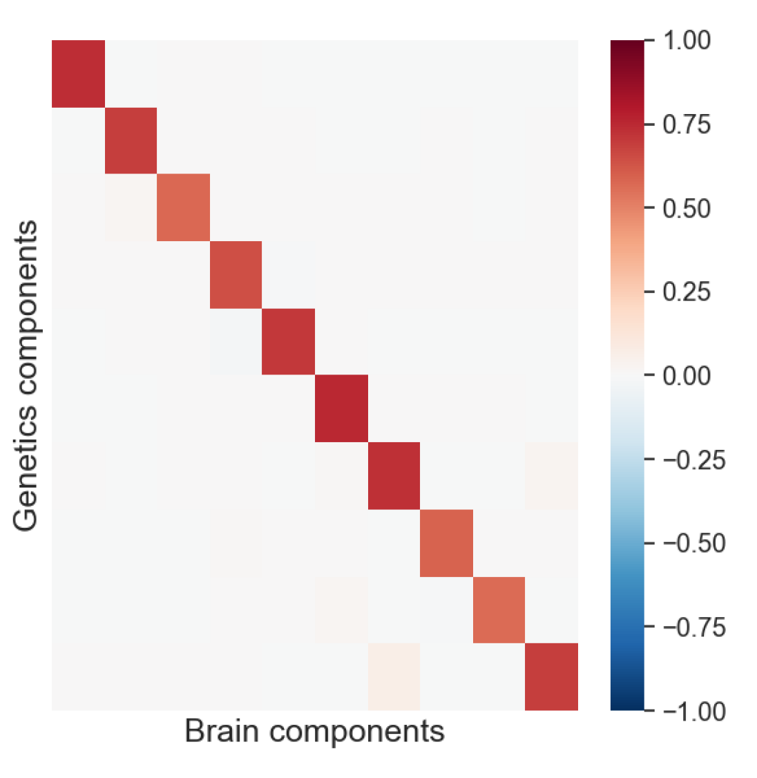
(a)

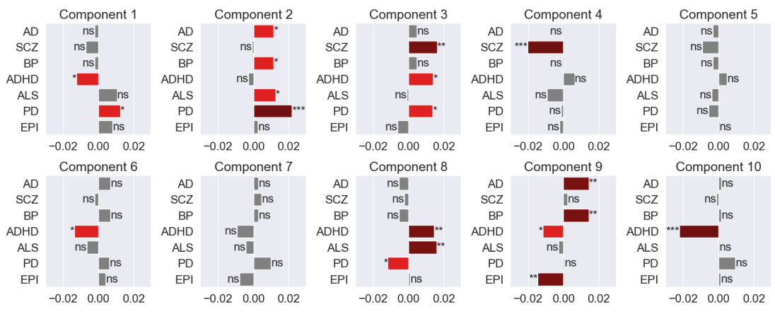
(b)

Figure 4: (a) Correlations between PLS components for UK Biobank. (b) Correlations between PLS brain components and genetic risk scores. AD=Alzheimer’s disease, SCZ=Schizophrenia, BP=Bipolar, ADHD=Attention deficit hyperactivity disorder, ALS=Amyotrophic lateral sclerosis, PD=Parkinson’s disease, EPI=Epilepsy. $\text{ns}:0.05<p<=1,\ast:0.01<p<=0.05,\ast\ast:0.001<p<=0.01,\ast\ast\ast:0.0001<p<=0.001$.

5.5 Self-Supervised Learning with SSL-EY

Finally, we benchmark our self-supervised learning algorithm, SSL-EY, with Barlow Twins and VICReg on CIFAR-10 and CIFAR-100. Each dataset contains 60,000 labelled images, but these are over 10 classes for CIFAR-10 and 100 classes for CIFAR-100.

We follow a standard experimental design (Tong et al., 2023). Indeed, we use the sololearn library (Da Costa et al., 2022), which offers optimized setups particularly tailored for VICReg and Barlow Twins. All methods utilize a ResNet-18 encoder coupled with a bi-layer projector network. Training spans 1,000 epochs with batches of 256 images. For SSL-EY, we use the hyperparameters optimized for Barlow Twins, aiming not to outperform but to showcase the robustness of our method. We predict labels via a linear probe on the learnt representations and evaluate performance with Top-1 and Top-5 accuracies on the validation set. For more details, refer to the supplementary material I.3.

Observations: Table 1 shows that SSL-EY is competitive with Barlow Twins and VICReg. This is remarkable because we used out-of-the-box hyperparameters for SSL-EY but used hyperparameters for Barlow Twins and VICReg that had been heavily optimized in previous studies.

Further experiments included in appendix H show that the learning curves for all three methods are comparable, and that our method is much more stable when reducing the dimension of the learnt representations.

Method	CIFAR-10 Top-1	CIFAR-10 Top-5	CIFAR-100 Top-1	CIFAR-100 Top-5
Barlow Twins	92.1	99.73	71.38	92.32
VICReg	91.68	99.66	68.56	90.76
SSL-EY	91.43	99.75	67.52	90.17

Table 1: Performance comparison of SSL methods on CIFAR-10 and CIFAR-100.

6 Conclusion

In this paper, we introduced a class of efficient, scalable algorithms for Canonical Correlation Analysis and Self-Supervised Learning, rooted in a novel unconstrained loss function. These algorithms are computationally lightweight, making them uniquely suited for large-scale problems where traditional methods struggle.

We have two distinct avenues for future research. Firstly, we aim to incorporate regularization techniques to improve both generalizability and interpretability, building upon existing sparse methods in CCA (Witten & Tibshirani, 2009). We also intend to investigate the utility of correlation as a metric for measuring the quality of learnt representations. This holds the potential to replace traditional validation methods like classification accuracy, especially in situations where validation labels are not available.

In summary, this paper sets a new benchmark for addressing large-scale CCA problems and opens new avenues in self-supervised learning, paving the way for more accessible and efficient solutions in various applications.

Appendix A Eckhart-Young characterization of GEP subspace

A.1 Formal definitions

There are various different notations and conventions for GEPs and SVDs. We largely follow the standard texts on Matrix Analysis (Stewart & Sun, 1990; Bhatia, 1997) but seek a more careful handling of the equality cases of certain results. To help, we use the following non-standard definitions, largely inspired by Carlsson (2021).

Definition A.1 (Top-$K$ subspace).

Let the GEP $(A,B)$ on $\mathbb{R}^{d}$ have eigenvalues $\lambda_{1}\geq\dots\geq\lambda_{d}$. Then a top-$K$ subspace is that spanned by some $w_{1},\dots,w_{K}$, where $w_{k}$ is a $\lambda_{i}$-eigenvector of $(A,B)$ for $k=1,\dots,K$.

Definition A.2 ($B$-orthonormality).

Let $B\in\mathbb{R}^{d\times d}$ be strictly positive definite. Then we say a collection $w_{1},\dots,w_{K}\in\mathbb{R}^{d}$ of vectors is $B$-orthonormal if $w_{k}^{T}Bw_{l}=\delta_{kl}$ for each $k,l\in\{1,\dots,K\}$.

Definition A.3 (Top-$K$ matrix).

We say $W\in\mathbb{R}^{d\times K}$ is a top-$K$ matrix for a GEP $(A,B)$ if the $k^{\text{th}}$ column $w_{i}$ of $W$ is a $\lambda_{k}$-eigenvector for each $k$ and the columns are $B$-orthonormal.

A.2 Standard Eckhart–Young inequality

Theorem A.1 (Eckhart–Young).

Let $M\in\mathbb{R}^{p\times q}$. Then $\hat{M}$ minimises $\|M-\tilde{M}\|_{F}$ over matrices $\tilde{M}$ of rank at most $K$ if and only if $\hat{M}=A_{K}R_{K}B_{K}^{\top}$ where $(A_{K},R_{K},B_{K})$ is some top-$K$ SVD of the target $M$.

Proof.

Let $M,\tilde{M}$ have singular values $\sigma_{k},\tilde{\sigma}_{k}$ respectively. Since $\tilde{M}$ has rank at most $K$ we must have $\tilde{\sigma}_{k}=0\text{ for }k>K$.

Then by von Neumann’s trace inequality (Carlsson, 2021),

$$\langle M,\tilde{M}\rangle_{F}\leq\sum_{k=1}^{K}\sigma_{k}\tilde{\sigma}_{k}$$

with equality if and only if $M,\tilde{M}$ ‘share singular vectors’; the notion of sharing singular vectors is defined as in Carlsson (2021) and in this case means that $\tilde{M}=A_{K}\tilde{R}_{K}B_{K}$ where $(A_{K},R_{K},B_{K})$ is some top-$K$ SVD of $M$ and $\tilde{R}_{K}$ is a diagonal matrix with decreasing diagonal elements $\tilde{\sigma}_{1}\geq\dots\geq\tilde{\sigma}_{K}$.

Expanding out the objective and applying this inequality gives

$$\lVert\tilde{M}-M\rVert_{F}^{2} \geq\sum_{k=1}^{d}\sigma_{k}^{2}-2\sum_{k=1}^{K}\sigma_{k}\tilde{\sigma}_{k}+\sum_{k=1}^{K}\tilde{\sigma}_{k}^{2}$$

$$=\sum_{k=K+1}^{d}\sigma_{k}^{2}+\sum_{k=1}^{K}(\sigma_{k}-\tilde{\sigma}_{k})^{2}$$

$$\geq\sum_{k=K+1}^{d}\sigma_{k}^{2}$$

so indeed to have equality in both cases requires $\sigma_{k}=\tilde{\sigma}_{k}$ for each $k\leq K$ so indeed $\tilde{R}_{K}=R_{K}$ and so $\hat{M}$, as defined in the statement of the theorem, minimises $\|M-\tilde{M}\|_{F}$ over matrices $\tilde{M}$ of rank at most $K$. ∎

A.3 Supporting Results

Lemma A.1 (Matrix square root lemma).

Suppose we have two full rank matrices $E,F\in\mathbb{R}^{d\times K}$ where $K\leq d$ and such that $EE^{T}=FF^{T}$; then there exists an orthogonal matrix $O\in\mathbb{R}^{K\times K}$ with $E=FO$.

Proof.

Post multiplying the defining condition gives $EE^{T}E=FF^{T}E$. Then right multiplying by $(E^{T}E)^{-1}$ gives

$$E=FF^{T}E(E^{T}E)^{-1}=\vcentcolon FO$$

to check that $O$ as defined above is orthogonal we again use the defining condition to compute

$$O^{T}O=(E^{T}E)^{-1}E^{T}FF^{T}E(E^{T}E)^{-1}=(E^{T}E)^{-1}E^{T}EE^{T}E(E^{T}E)^{-1}=I_{K}$$

∎

Corollary A.1 (PSD Eckhart–Young for square root matrix).

Let $M\in\mathbb{R}^{d\times d}$ be symmetric positive semidefinite. Then

$$\operatorname*{arg\,min}_{\tilde{Z}\in\mathbb{R}^{d\times K}}\|M-\tilde{Z}\tilde{Z}^{T}\|_{F}^{2}$$

is precisely the set of $\tilde{Z}$ of the form $\tilde{Z}=Z_{K}\Lambda_{K}^{\nicefrac{{1}}{{2}}}O_{K}$ for some top-$K$ eigenvector-matrix $Z_{K}$ of the GEP $(M,I)$ and some orthogonal $O_{K}\in\mathcal{O}(K)$, and where $\Lambda_{K}$ is a diagonal matrix of the top-$K$ eigenvalues.

Proof.

First note that when $M$ is positive semi-definite the SVD coincides with the eigendecomposition.

Second note that taking $\tilde{Z}=Z_{K}\Lambda_{K}^{\nicefrac{{1}}{{2}}}O_{K}$ attains the minimal value by the Eckhart–Young inequality, Theorem A.1.

Next note that if $\tilde{Z}$ attains the minimal value then it must have $\tilde{Z}\tilde{Z}^{T}=Z_{K}\Lambda_{K}Z_{K}^{T}$ by the equality case of Eckhart–Young. Then by matrix square root Lemma A.1 we must indeed have $\tilde{Z}=Z_{K}\Lambda_{K}^{\nicefrac{{1}}{{2}}}O_{K}$ for some orthogonal $O_{K}$. ∎

Corollary A.2 (Symmetric Eckhart–Young for square root matrix).

Let $M\in\mathbb{R}^{d\times d}$ be symmetric with eigenvalues $\lambda_{1}\geq\dots\geq\lambda_{d}$ such that $\lambda_{K}>0$. Then

$$\operatorname*{arg\,min}_{\tilde{Z}\in\mathbb{R}^{d\times K}}\|M-\tilde{Z}\tilde{Z}^{T}\|_{F}^{2}$$

is precisely the set of $\tilde{Z}$ of the form $\tilde{Z}=Z_{K}\Lambda_{K}^{\nicefrac{{1}}{{2}}}O_{K}$ for some top-$K$ eigenvector-matrix $Z_{K}$ of the GEP $(M,I)$ and some orthogonal $O_{K}\in\mathcal{O}(K)$, and where $\Lambda_{K}$ is a diagonal matrix of the top-$K$ eigenvalues.

Proof.

Let $\tilde{Z}\in\mathbb{R}^{d\times K}$. Because $M$ is symmetric it has some eigen-decomposition; separate this into strictly positive and non-positive eigenvalues $M=M_{+}+M_{-}=Z_{+}\Lambda_{+}Z_{+}^{T}+Z_{-}\Lambda_{-}Z_{-}^{T}$, with rank $d_{+},d_{-}$ respectively. Let the corresponding projections be $P_{+}=Z_{+}Z_{+}^{T},P_{-}=Z_{-}Z_{-}^{T}$.

Now define $\tilde{Z}_{+}=P_{+}\tilde{Z},\tilde{Z}_{-}=P_{-}\tilde{Z}$. Then note by orthogonality of the projections we have for any matrix $A$ that

$$\lVert A\rVert^{2}=\lVert(P_{+}+P_{-})A(P_{+}+P_{-})\rVert^{2}=\lVert P_{+}AP_{+}\rVert^{2}+\lVert P_{+}AP_{-}\rVert^{2}+\lVert P_{-}AP_{+}\rVert^{2}+\lVert P_{-}AP_{-}\rVert^{2}$$

So we can expand out

$$\lVert M-\tilde{Z}\tilde{Z}^{T}\rVert^{2} =\lVert(P_{+}+P_{-})(M-\tilde{Z}\tilde{Z}^{T})(P_{+}+P_{-})\rVert^{2}$$

$$=\underbrace{\lVert M_{+}-\tilde{Z}_{+}\tilde{Z}_{+}^{T}\rVert^{2}}_{\geq\sum_{k=K+1}^{d_{+}}\lambda_{k}^{2}}+\underbrace{\lVert M_{-}-\tilde{Z}_{-}\tilde{Z}_{-}^{T}\rVert^{2}}_{\geq\lVert M_{-}\rVert^{2}}+\underbrace{\lVert\tilde{Z}_{+}\tilde{Z}_{-}^{T}\rVert^{2}}_{\geq 0}+\underbrace{\lVert\tilde{Z}_{-}\tilde{Z}_{+}^{T}\rVert^{2}}_{\geq 0}\geq\sum_{k=K+1}^{d}\lambda_{k}^{2}$$ (14)

where the first inequality follows from the previous Corollary A.1 and the second inequality is just from

$$\lVert M_{-}-\tilde{Z}_{-}\tilde{Z}_{-}^{T}\rVert^{2}-\lVert M_{-}\rVert^{2}=-2\operatorname{trace}\left(\tilde{Z}_{-}^{T}M_{-}\tilde{Z}_{-}\right)+\lVert\tilde{Z}_{-}\tilde{Z}_{-}^{T}\rVert^{2}\geq 0$$

because $M_{-}$ has negative eigenvalues.

Moreover equality in (14) requires the equality case of all the component inequalities; the first gives $\tilde{Z}_{+}=Z_{K}\Lambda_{K}^{\nicefrac{{1}}{{2}}}O_{K}$ for some $Z_{K},O_{K}$ as in the statement of Corollary A.1, and the second that $\tilde{Z}_{-}=0$; so indeed combining $\tilde{Z}=\tilde{Z}_{+}+\tilde{Z}_{-}$ gives the result. ∎

A.4 GEP-EY Objective

Proposition A.1 (GEP-EY-Objective).

Consider the GEP $(A,B)$ with $A$ symmetric and $B$ positive definite; suppose there are at least $K$ strictly positive (generalized) eigenvalues. Then:

$$\tilde{W}\in\operatorname*{arg\,max}_{\tilde{W}\in\mathbb{R}^{d\times k}}\>\operatorname{trace}\left\{2\left(\tilde{W}^{T}A\tilde{W}\right)-\left(\tilde{W}^{T}B\tilde{W}\right)\left(\tilde{W}^{T}B\tilde{W}\right)\right\}$$

if and only if $\tilde{W}=W_{K}\Lambda_{K}^{\nicefrac{{1}}{{2}}}O_{K}$ for some top-$K$ matrix $W_{K}$ of the GEP and some orthogonal $O_{K}\in\mathcal{O}(k)$, where $\Lambda_{K}$ is a diagonal matrix of the top-$K$ eigenvalues.

Moreover, the maximum value is precisely $\sum_{k=1}^{K}\lambda_{k}^{2}$.

Proof.

First recall that there is a bijection between eigenvectors $w$ for the GEP $(A,B)$ and eigenvectors $z=B^{\nicefrac{{1}}{{2}}}w$ for the GEP $(M,I)$ where $M\vcentcolon=B^{\shortminus\nicefrac{{1}}{{2}}}AB^{\shortminus\nicefrac{{1}}{{2}}}$ (e.g. see Chapman et al. (2022)).

Now consider how the Eckhart–Young objective from Corollary A.2 transforms under the bijection $Z=B^{\nicefrac{{1}}{{2}}}W$.

We get

$$\|M-\tilde{Z}\tilde{Z}\|_{F}^{2} =\|B^{\shortminus\nicefrac{{1}}{{2}}}AB^{\shortminus\nicefrac{{1}}{{2}}}-B^{\nicefrac{{1}}{{2}}}\tilde{W}\tilde{W}^{T}B^{\nicefrac{{1}}{{2}}}\|_{F}^{2}$$

$$=\|B^{\shortminus\nicefrac{{1}}{{2}}}AB^{\shortminus\nicefrac{{1}}{{2}}}\|_{F}^{2}-2\operatorname{trace}\left(B^{\shortminus\nicefrac{{1}}{{2}}}AB^{\shortminus\nicefrac{{1}}{{2}}}B^{\nicefrac{{1}}{{2}}}\tilde{W}\tilde{W}^{T}B^{\nicefrac{{1}}{{2}}}\right)$$

$$\quad+\operatorname{trace}\left(B^{\nicefrac{{1}}{{2}}}\tilde{W}\tilde{W}^{T}B^{\nicefrac{{1}}{{2}}}\>B^{\nicefrac{{1}}{{2}}}\tilde{W}\tilde{W}^{T}B^{\nicefrac{{1}}{{2}}}\right)$$

$$=\|B^{\shortminus\nicefrac{{1}}{{2}}}AB^{\shortminus\nicefrac{{1}}{{2}}}\|_{F}^{2}-\operatorname{trace}\left\{2\left(\tilde{W}^{T}A\tilde{W}\right)-\left(\tilde{W}^{T}B\tilde{W}\right)\left(\tilde{W}^{T}B\tilde{W}\right)\right\},$$

where the first term is independent of $\tilde{W}$, so we can conclude by Corollary A.2.

The moreover conclusion can follow from computing the objective at any maximiser of the form above. We note that

$$\tilde{W}^{T}A\tilde{W} =O_{K}^{T}\Lambda_{K}^{\nicefrac{{1}}{{2}}}W_{K}^{T}AW_{K}\Lambda_{K}O_{K}=O_{K}^{T}\Lambda_{K}^{2}O_{K}$$

$$\tilde{W}^{T}B\tilde{W} =O_{K}^{T}\Lambda_{K}^{\nicefrac{{1}}{{2}}}W_{K}^{T}BW_{K}\Lambda_{K}O_{K}=O_{K}^{T}\Lambda_{K}O_{K}$$

plugging into the objective gives

$$\operatorname{trace}\left(2\>(\tilde{W}^{T}A\tilde{W})-(\tilde{W}^{T}B\tilde{W})^{2}\right)=\operatorname{trace}\left(2\,O_{K}^{T}\Lambda_{K}^{2}O_{K}-O_{K}^{T}\Lambda_{K}^{2}O_{K}\right)=\sum_{k=1}^{K}\lambda_{k}^{2}$$

because the trace of a symmetric matrix is equal to the sum of its eigenvalues. ∎

A.5 Alternative unconstrained objective for CCA from SVD formulation

Proposition A.2 (CCA-SVD-Objective).

Consider the CCA problem defined by $X,Y\in\mathbb{R}^{p},\mathbb{R}^{q}$; suppose there are at least $K$ strictly positive canonical correlations. Then

$$(\tilde{U},\tilde{V})\in\operatorname*{arg\,min}_{\tilde{U}\in\mathbb{R}^{p\times K},\tilde{V}\in\mathbb{R}^{q\times K}}\operatorname{trace}\left\{2\,\left({\tilde{U}}^{T}\Sigma_{xy}{\tilde{V}}\right)-\left(\,{\tilde{U}}^{T}\Sigma_{xx}{\tilde{U}}\right)\>\left({\tilde{V}}^{T}\Sigma_{yy}{\tilde{V}}\,\right)\right\}$$ (15)

if and only if $\tilde{U}=U_{K}R_{K}^{\nicefrac{{1}}{{2}}}S_{K}$, $\tilde{V}=V_{K}R_{K}^{\nicefrac{{1}}{{2}}}T_{K}$ where $(U_{K},V_{K},R_{K})$ is a top-$K$ CCA solution and $S_{K}T_{K}^{T}=I_{K}$.

Moreover, the minimum value is precisely $\sum_{k=1}^{K}\rho_{k}^{2}$

Proof.

It is well known that CCA can be characterized as a SVD of $M\vcentcolon=\Sigma_{xx}^{\shortminus\nicefrac{{1}}{{2}}}\Sigma_{xy}\Sigma_{yy}^{\nicefrac{{1}}{{2}}}$; in particular if $u_{k},v_{k},\rho_{k}$ are the canonical directions and correlations respectively then the $a_{k}\vcentcolon=\Sigma_{xx}^{\nicefrac{{1}}{{2}}}u_{k},b_{k}\vcentcolon=\Sigma_{yy}^{\nicefrac{{1}}{{2}}}v_{k},\rho_{k}$ are the left and right singular vectors and singular values respectively. As always, we assume $\Sigma_{xx},\Sigma_{yy}$ invertible so there is a bijection between CCA solutions and SVD solutions; this is the key to the argument below. We will also express this bijection implicitly with letters for matrices, setting $A_{K}\vcentcolon=\Sigma_{xx}^{\nicefrac{{1}}{{2}}}U_{K},B_{K}\vcentcolon=\Sigma_{yy}^{\nicefrac{{1}}{{2}}}V_{K}$, $\tilde{A}=\Sigma_{xx}^{\nicefrac{{1}}{{2}}}\tilde{U},\tilde{B}=\Sigma_{yy}^{\nicefrac{{1}}{{2}}}\tilde{V}$.

Applying Eckhart–Young theorem A.1 to this target matrix $M$ therefore shows

$$\lVert M-\tilde{A}\tilde{B}^{T}\rVert^{2}\geq\sum_{k=K+1}^{p}\rho_{k}^{2}=\lVert M\rVert^{2}-\sum_{k=1}^{K}\rho_{k}^{2}$$

with equality if and only if $\tilde{A}\tilde{B}^{T}=A_{K}R_{K}B_{K}^{T}$ for some top-$K$ SVD matrices $A_{K},B_{K}$.

This Eckhart–Young objective is (up to the constant of $\lVert M\rVert^{2}=\sum\rho_{k}^{2}$) equivalent to our stated objective:

$$\lVert M-\tilde{A}\tilde{B}^{T}\rVert^{2} =\lVert\Sigma_{xx}^{\shortminus\nicefrac{{1}}{{2}}}\Sigma_{xy}\Sigma_{yy}^{\nicefrac{{1}}{{2}}}-\Sigma_{xx}^{\nicefrac{{1}}{{2}}}-\Sigma_{xx}^{\nicefrac{{1}}{{2}}}\tilde{U}\tilde{V}^{T}\Sigma_{yy}^{\nicefrac{{1}}{{2}}}\rVert$$

$$=\lVert\Sigma_{xx}^{\shortminus\nicefrac{{1}}{{2}}}\Sigma_{xy}\Sigma_{yy}^{\shortminus\nicefrac{{1}}{{2}}}\rVert^{2}-2\langle\Sigma_{xx}^{\shortminus\nicefrac{{1}}{{2}}}\Sigma_{xy}\Sigma_{yy}^{\shortminus\nicefrac{{1}}{{2}}},\Sigma_{xx}^{\nicefrac{{1}}{{2}}}\tilde{U}\tilde{V}^{T}\Sigma_{yy}^{\nicefrac{{1}}{{2}}}\rangle+\lVert\Sigma_{xx}^{\nicefrac{{1}}{{2}}}\tilde{U}\tilde{V}^{T}\Sigma_{yy}^{\nicefrac{{1}}{{2}}}\rVert^{2}$$

$$=\lVert M\rVert^{2}-2\operatorname{trace}\left(\tilde{U}^{T}\Sigma_{xy}\tilde{V}\right)+\operatorname{trace}\left(\tilde{U}^{T}\Sigma_{xx}\tilde{U}\>\tilde{V}^{T}\Sigma_{yy}\tilde{V}\right)$$

Moreover, transforming with the bijection back to CCA perspective, we have equality if and only if there is some $U_{K},V_{K}$ such that

$$\tilde{A}\tilde{B}^{T}=A_{K}R_{K}B_{K}^{T}\implies\tilde{U}\tilde{V}^{T}=U_{K}R_{K}V_{K}^{T}$$

this second equality in fact gives the equality case of the claim. Indeed, $U_{K},\tilde{U}$, $V_{K},\tilde{V}$ respectively must have the same column spaces, and $R_{K}$ is invertible, so we can write $\tilde{U}=U_{K}R_{K}^{\nicefrac{{1}}{{2}}}S_{K}$, $\tilde{V}=V_{K}R_{K}^{\nicefrac{{1}}{{2}}}T_{K}$ for some invertible matrices $S_{K},T_{K}$. Then

$$U_{K}^{T}\tilde{U}\tilde{V}V_{K}=R_{K}\implies R_{K}^{\nicefrac{{1}}{{2}}}S_{K}T_{K}^{T}R_{K}^{\nicefrac{{1}}{{2}}}=R_{K}\implies S_{K}T_{K}^{T}=I_{K}$$

as required.

It is instructive to further compute the individual components of this expression at the optimal values. We obtain:

$$\tilde{U}^{T}\Sigma_{xy}\tilde{V}=S_{K}^{T}R_{K}^{\nicefrac{{1}}{{2}}}U_{K}^{T}\Sigma_{xy}V_{K}R_{K}^{\nicefrac{{1}}{{2}}}T_{K}=S_{K}^{T}R_{K}^{2}T_{K}$$

$$\tilde{U}^{T}\Sigma_{xx}\tilde{U}=S_{K}^{T}R_{K}^{\nicefrac{{1}}{{2}}}U_{K}^{T}\Sigma_{xx}U_{K}R_{K}^{\nicefrac{{1}}{{2}}}S_{K}=S_{K}^{T}R_{K}S_{K}$$

$$\tilde{V}^{T}\Sigma_{yy}\tilde{V}=T_{K}^{T}R_{K}^{\nicefrac{{1}}{{2}}}V_{K}^{T}\Sigma_{yy}V_{K}R_{K}^{\nicefrac{{1}}{{2}}}T_{K}=T_{K}^{T}R_{K}T_{K}^{T}$$

so by cyclicity of trace, the value of the objective becomes

$$\operatorname{trace}2\,S_{K}R_{K}^{2}T_{K}-S_{K}^{T}R_{K}S_{K}T_{K}^{T}R_{K}T_{K}=\operatorname{trace}2R_{K}^{2}-R_{K}^{2}=\operatorname{trace}R_{K}^{2}=\sum_{k=1}^{K}\rho_{k}^{2}$$

we observe that though this ultimate objective is in a nice form, the individual $\tilde{U},\tilde{V}$ are much harder to interpret due to the confounding by arbitrary invertible matrices $S_{K},T_{K}$. ∎

Appendix B Tractable Optimization - no spurious local minima

First in section B.1 we prove that for general $A,B$ our loss $\mathcal{L}_{\text{EY}}(U)$ has no spurious local minima. Then in section B.2 we apply a result from Ge et al. (2017). This application is somewhat crude, and we expect that a quantitative result with tighter constants could be obtained by adapting the argument of section B.1; we leave such analysis to future work.

B.1 Qualitative results

First we prove an auxillary result.

Lemma B.1.

Let $M\in\mathbb{R}^{D\times D}$ be a symmetric matrix and let $U\in\mathbb{R}^{D\times K}$. Let

$$\hat{\Gamma}\vcentcolon=\operatorname*{arg\,min}_{\Gamma\in\mathbb{R}^{K\times K}}\lVert M-U\Gamma U^{T}\rVert_{F}^{2}$$

Then $U\hat{\Gamma}U^{T}=\mathcal{P}_{U}M\mathcal{P}_{U}$ and the minimum value is precisely

$$\lVert M\rVert_{F}^{2}-\lVert\mathcal{P}_{U}M\mathcal{P}_{U}\rVert_{F}^{2}$$ (16)

Moreover, if $U$ has orthonormal columns then $\hat{\Gamma}=U^{T}MU$, and $\lVert\mathcal{P}_{U}M\mathcal{P}_{U}\rVert_{F}^{2}=\lVert\hat{\Gamma}\rVert_{F}^{2}$

Proof.

Simply complete the square to give

$$\lVert M-U\Gamma U^{T}\rVert_{F}^{2} =\operatorname{trace}(U^{T}U)\Gamma^{T}(U^{T}U)\Gamma-2\operatorname{trace}D(U^{T}MU)+\lVert M\rVert_{F}^{2}$$

$$=\lVert(U^{T}U)^{\nicefrac{{1}}{{2}}}\Gamma(U^{T}U)^{\nicefrac{{1}}{{2}}}-(U^{T}U)^{\shortminus\nicefrac{{1}}{{2}}}(U^{T}MU)(U^{T}U)^{\shortminus\nicefrac{{1}}{{2}}}\rVert_{F}^{2}+\lVert M\rVert_{F}^{2}-\lVert\mathcal{P}_{U}M\mathcal{P}_{U}\rVert_{F}^{2}$$

from which we can read off that the minimum is attained precisely when

$$\Gamma=(U^{T}U)^{-1}(U^{T}MU)(U^{T}U)^{-1}$$

and that the optimal value is precisely the value of eq. 16 as claimed. Finally, if $U$ has orthonormal columns, $U^{T}U=I_{K}$ so $\Gamma^{*}$ is of the form claimed, and the final equality comes from expanding out the trace form of the Frobenius norm. ∎

Lemma B.2.

Let $M\in\mathbb{R}^{D\times D}$ be a symmetric matrix and $\mathcal{U}$ a subspace of $\mathbb{R}^{D}$ of dimension $L$. Then there exists an orthonormal basis $u_{1},\dots,u_{L}$ for $\mathcal{U}$ such that

$$u_{L}\perp Mu_{l}\>\text{ for }l\in\{1,\dots,L-1\}$$

Proof.

Consider the action of $\tilde{M}\vcentcolon=\mathcal{P}_{\mathcal{U}}M\mathcal{P}_{\mathcal{U}}$ on $\mathcal{U}$. Then $\tilde{M}$ is symmetric matrix whose range is a subspace of $\mathcal{U}$ and so there exists an orthonormal set of eigenvectors $u_{1},\dots,u_{L}$ that give a basis for $\mathcal{U}$ with corresponding eigenvalues $\tilde{\lambda}_{1}\geq\dots\geq\tilde{\lambda}_{L}$. Then we can read off

$$\langle u_{L},Mu_{l}\rangle=\langle u_{L},\tilde{M}u_{l}\rangle=\tilde{\lambda}_{l}\langle u_{L},u_{l}\rangle=0$$

as required. ∎

Proposition B.1 (No spurious local minima).

The (population) objective $\mathcal{L}^{EY}$ has no spurious local minima. That is, any matrix $\bar{W}$ that is a local minimum of $\mathcal{L}^{EY}$ must in fact be a global minimum of the form described in proposition 3.1.

Proof.

We shall show that for any matrix $W$ that is not a global optimum, there is a (continuous) path of solutions $W_{t}$ with:

$$W_{0}=W,\quad W_{1}=\hat{W},\quad W_{t}\to W\text{ as }t\to 0,\quad\text{and}\quad\mathcal{L}^{EY}(W_{t})<\mathcal{L}^{EY}(W)\>\forall t>0$$

As in the proof of proposition 3.1 we first reduce to the $B=I$ setting by defining $Z\vcentcolon=B^{{\shortminus\nicefrac{{1}}{{2}}}}W$ and $M=B^{\shortminus\nicefrac{{1}}{{2}}}AB^{\shortminus\nicefrac{{1}}{{2}}}$. Let the eigendecomposition of $M$ be $M=V^{*}D^{*}{V^{*}}^{\top}$. Define the loss

$$l(Z)\vcentcolon=\lVert M-ZZ^{\top}\rVert_{F}^{2}$$

It is now sufficient to show that: for any matrix $Z\in\mathbb{R}^{D\times K}$ that is not of the form $V^{*}_{K}D^{*}_{K}O_{K}$ where $V^{*}_{K}$ is a matrix whose columns are a set of top-$K$ eigenvectors for $M$, and $O_{K}\in\mathbb{R}^{K\times K}$ is some arbitrary orthogonal matrix cannot be a local minimum.

For notational simplicity we will assume that the $\lambda_{K}(M)>\lambda_{K+1}(M)$ from now on, such that $V_{K}^{*}$ can be made well-defined.

Now, take such a $Z$ and suppose, for contradiction that it is a local minimum. We will construct a continuous path of matrices $Z(t):t\in[0,1]$ with $Z(0)=Z$ and $l\left(Z(t)\right)<l(Z)\>\forall t>0$.

Then by our assumption on the form of $Z$, we have

$$\mathcal{V}_{K}\vcentcolon={\operatorname{span}\{{Z}\}}\neq{\operatorname{span}\{{V_{K}^{*}}\}}=\vcentcolon\mathcal{V}^{*}_{K}$$

Now comes the clever part of the proof. Define $\kappa_{\cap}=\operatorname{dim}{\operatorname{span}\{{\mathcal{V}_{K}\cap\mathcal{V}_{K}^{*}}\}}$. Then pick orthonormal bases

• $u_{1},\dots,u_{\kappa_{\cap}}$ for $\mathcal{V}_{K}\cap\mathcal{V}_{K}^{*}$

• $u_{\kappa_{\cap}+1},\dots,u_{K}$ for $\mathcal{V}_{K}\cap\mathcal{V}_{K}^{*}$ such that $u_{K}\perp Mu_{k}$ for all $k=\kappa_{\cap}+1,\dots,K-1$ by lemma B.2

• $u^{*}_{\kappa_{\cap}+1},\dots,u^{*}_{K}$ for $\mathcal{V}_{K}^{*}\cap\mathcal{V}_{K}$

Let $U_{K}=\begin{pmatrix}u_{1}&\dots&u_{K}\end{pmatrix}$. Then by lemma B.1, for $Z$ to be a local minimum we must have

$$ZZ^{T}=U_{K}(U_{K}^{T}MU_{K})U_{K}^{T}$$

Moreover the objective value must therefore be

$$l(Z)=\lVert M\rVert_{F}^{2}-\lVert U_{K}^{T}MU_{K}\rVert_{F}^{2}$$ (17)

We now make the observation that the second term is the ‘signal of $M$ captured by the subspace of $U_{K}$’. So aligning $U_{K}$ with higher-eigenvalue subspaces of $M$ should increase this amount of signal captured and decrease this loss.

We now construct a path $U_{K}(t)$ which captures this intuition.

Let $u_{K}(t)=\cos(t)u_{K}+\sin(t)u^{*}_{K}$. Then let $U_{K}(t)$ have columns $u_{1},\dots,u_{K-1},u_{K}(t)$. By construction this is still an orthonormal set of basis vectors, so $U_{K}(t)^{T}U_{K}=I_{K}$. Let $\Gamma(t)=U_{K}(t)^{T}MU_{K}(t)$.

We are finally ready to construct the path $Z(t)$. Because $U_{K}$ is a basis for the column space of $Z$, and $Z$ is assumed to be a local optimum, we must have

$$ZZ^{T}=U_{K}\Gamma(0)U_{K}^{T}$$

by lemma B.1. So $Z=U_{K}\Gamma^{\nicefrac{{1}}{{2}}}O_{K}$ for some orthogonal matrix $O_{K}\in\mathbb{R}^{K\times K}$ where $\Gamma^{\nicefrac{{1}}{{2}}}$ is the unique positive semi-definite square root of $\Gamma$. So define

$$Z(t)=U_{K}(t)\Gamma(t)^{\nicefrac{{1}}{{2}}}O_{K}$$

where again $\Gamma(t)^{\nicefrac{{1}}{{2}}}$ is the unique positive semi-definite square root and therefore both $U_{k}(t)$ and $\Gamma(t)^{\nicefrac{{1}}{{2}}}$ are continuous functions of $t$ and therefore so is $Z$.

Then

$$l(Z(t))=\lVert M\rVert_{F}^{2}-\lVert U_{K}(t)^{T}MU_{K}(t)\rVert_{F}^{2}$$ (18)

So it is sufficient to show that $\lVert U_{K}(t)^{T}MU_{K}(t)\rVert_{F}^{2}>\lVert U_{K}^{T}MU_{K}\rVert_{F}^{2}$ for $t\in[0,\pi/2]$. Indeed, we can compute

$$\lVert U_{K}(t)^{T}MU_{K}(t)\rVert_{F}^{2}-\lVert U_{K}^{T}MU_{K}\rVert_{F}^{2} =\left(u_{K}(t)^{T}Mu_{K}(t)\right)^{2}-\left(u_{K}^{T}Mu_{K}\right)^{2}$$

$$\quad+2\sum_{k=1}^{K-1}\left\{\left(u_{K}(t)^{T}Mu_{k}\right)^{2}-\left(u_{K}^{T}Mu_{k}\right)^{2}\right\}$$

$$\geq\left(u_{K}(t)^{T}Mu_{K}(t)\right)^{2}-\left(u_{K}^{T}Mu_{K}\right)^{2}$$

because $u_{K}^{T}Mu_{k}=0$ for $k=1,\dots,K-1$ by construction. Finally we have

$$u_{K}(t)^{T}Mu_{K}(t) =\sin^{2}(t)\langle u_{K}^{*},Mu_{K}^{*}\rangle+2\sin(t)\cos(t)\langle u_{K},Mu_{K}^{*}\rangle+\cos^{2}(t)\langle u_{K},Mu_{K}\rangle$$

$$=\sin^{2}(t)\langle u_{K}^{*},Mu_{K}^{*}\rangle+\cos^{2}(t)\langle u_{K},Mu_{K}\rangle$$

$$>u_{K}^{T}Mu_{K}$$

Here we used that $\langle u_{K}^{*},Mu_{K}^{*}\rangle\geq\lambda_{K}>\langle u_{K},Mu_{K}\rangle$ and that the middle term vanishes because $Mu_{K}^{*}\in\mathcal{U}^{*}_{K}$ and is therefore orthogonal to $u_{K}$.

∎

B.2 Quantitative results

To use the results from Ge et al. (2017) we need to introduce their definition of a $(\theta,\gamma,\zeta)$-strict saddle.

Definition B.1.

We say function $l(\cdot)$ is a $(\theta,\gamma,\zeta)$-strict saddle if for any $x$, at least one of the following holds:

1. $\lVert\nabla l(x)\rVert\geq\theta$

2. $\lambda_{\text{min}}(\nabla^{2}l(x))\leq-\gamma$

3. $x$ is $\zeta$-close to $\mathcal{X}^{*}$ - the set of local minima.

.

We can now state restate Lemma 13 from Ge et al. (2017) in our notation; this was used in their analysis of robust PCA, and directly applies to our PCA-type formulation.

Lemma B.3 (Strict saddle for PCA).

Let $M\in\mathbb{R}^{D\times D}$ be a symmetric PSD matrix, and define the matrix factorization objective over $Z\in\mathbb{R}^{D\times K}$

$$l(Z)=\lVert M-ZZ^{\top}\rVert^{2}$$

Assume that $\lambda^{*}_{K}\vcentcolon=\lambda_{K}(M)\geq 15\lambda_{K+1}(M)$. Then

1. all local minima satisfy $ZZ^{T}=\mathcal{P}_{K}(M)$ - the best rank-$K$ approximation to $M$

2. the objective l(Z) is $(\epsilon,\Omega(\lambda_{K}^{*}),\mathcal{O}(\epsilon/\lambda_{K}^{*})$-strict saddle.

However, we do not want to show a strict saddle of $l$ but of $\mathcal{L}_{\text{EY}}:U\mapsto l(B^{\nicefrac{{1}}{{2}}}U)$. Provided that $B$ has strictly positive minimum and bounded maximum eigenvalues this implies that $\mathcal{L}_{\text{EY}}$ is also strict saddle, as we now make precise.

Lemma B.4 (Change of variables for strict saddle conditions).

Suppose that $l$ is $(\theta,\gamma,\zeta)$-strict saddle and let $L:U\mapsto l(B^{\nicefrac{{1}}{{2}}}U)$ for $B$ with minimal and maximal eigenvalues $\sigma_{\text{min}},\sigma_{\text{max}}$ respectively.

Then $L$ is $\left(\sigma_{\text{max}}^{\nicefrac{{1}}{{2}}}\theta,\,\sigma_{\text{min}}\gamma,\,\sigma_{\text{max}}^{\nicefrac{{1}}{{2}}}\zeta\right)$-strict saddle.

Proof.

Write $g(U)=B^{\nicefrac{{1}}{{2}}}U$. Then $L=l\circ g$, so by the chain rule:

$$D_{U}L=D_{B^{\nicefrac{{1}}{{2}}}U}l\circ D_{U}g\,:\>\delta U\mapsto\langle\nabla l(B^{\nicefrac{{1}}{{2}}}U),B^{{\nicefrac{{1}}{{2}}}}\delta U\rangle=\langle B^{\nicefrac{{1}}{{2}}}\nabla l(B^{\nicefrac{{1}}{{2}}}U),\delta U\rangle$$

Therefore

$$\lVert\nabla L(U)\rVert=\lVert B^{\nicefrac{{1}}{{2}}}\nabla l(B^{\nicefrac{{1}}{{2}}}U)\rVert\geq\sigma_{\text{min}}^{\nicefrac{{1}}{{2}}}\lVert l(B^{\nicefrac{{1}}{{2}}}U)\rVert$$

By a further application of the chain rule we have

$$D_{U}^{2}L\,:\>\delta U,\delta U\mapsto D^{2}_{B^{\nicefrac{{1}}{{2}}}U}l(B^{\nicefrac{{1}}{{2}}}\delta U,B^{\nicefrac{{1}}{{2}}}\delta U)$$

Suppose $\lambda_{\text{min}}(\nabla^{2}l(Z))\leq-\gamma$ then by the variational characterization of eigenvalues, there exists some $\delta Z$ such that $\langle\delta Z,\nabla^{2}l(Z)\delta Z\rangle\leq-\gamma\lVert\delta Z\rVert^{2}$. Then taking $\delta U=B^{\shortminus\nicefrac{{1}}{{2}}}\delta Z$ gives

$$\langle\delta U,\nabla^{2}L(U)\delta U\rangle =\langle B^{\nicefrac{{1}}{{2}}}\delta U,\nabla^{2}l(B^{\nicefrac{{1}}{{2}}}U)B^{\nicefrac{{1}}{{2}}}\delta U\rangle$$

$$=\langle\delta Z,\nabla^{2}l(Z)\delta Z\rangle$$

$$\leq-\gamma\lVert\delta Z\rVert^{2}$$

$$\leq-\gamma\sigma_{\text{min}}\lVert\delta U\rVert^{2}$$

Thirdly, suppose that $\lVert B^{\nicefrac{{1}}{{2}}}U-Z^{*}\rVert\leq\zeta$ for some local optimum $Z^{*}$ of $l$. Then since $B$ is invertible, $U^{*}\vcentcolon=B^{\shortminus\nicefrac{{1}}{{2}}}Z^{*}$ is a local optimum of $L$. In addition:

$$\lVert U-U^{*}\rVert=\lVert B^{\nicefrac{{1}}{{2}}}(U-U^{*})\rVert\leq\sigma_{\text{max}}^{\nicefrac{{1}}{{2}}}\lVert B^{\nicefrac{{1}}{{2}}}U-Z^{*}\rVert\leq\zeta$$

Finally, consider some arbitrary point $U_{0}$. Let $Z_{0}=B^{\nicefrac{{1}}{{2}}}U_{0}$. Then by the strict saddle property for $l$ one of the following must hold:

1. $\lVert\nabla l(Z_{0})\rVert\geq\theta\quad\implies\quad\lVert\nabla L(U_{0})\rVert\geq\sigma_{\text{min}}^{\nicefrac{{1}}{{2}}}\theta$

2. $\lambda_{\text{min}}(\nabla^{2}l(Z_{0}))\leq-\gamma\quad\implies\quad\lambda_{\text{min}}(\nabla^{2}L(U_{0})\leq-\sigma_{\text{min}}\gamma$

3. $Z_{0}$ is $\zeta$-close to a local-minimum $Z^{*}$, which implies that $U_{0}$ is $(\sigma_{\text{max}}^{\nicefrac{{1}}{{2}}}\zeta)$-close to a local minimum $B^{\shortminus\nicefrac{{1}}{{2}}}Z^{*}$ of $L$.

∎

By combining lemma B.3 with lemma B.4, we can conclude that our objective does indeed satisfy a (quantitative) strict saddle property. This is sufficient to show that certain local search algorithms will converge in polynomial time Ge et al. (2017).

However, this version of the strict saddle property is not quite enough to prove the claim for stochastic gradient descent (SGD). Certain extra conditions are given in Ge et al. (2015) to guarantee polynomial time convergence of noisy SGD. These are: 1. a notion of local strict convexity near any local minima, and 2. boundedness assumptions. The first assumption is easy to show in our setting, but the second clearly fails. That being said, we could approximate the objective by mollifying it to be bounded outside a large ball. Then it should be straightforward to use a supermartingale argument to show that with high probability the sample paths are contained within said ball; and then inherit convergence guarantees from the bounded case.

Appendix C Further CCA background

C.1 Eckhart-Young loss recovers Deep CCA

See 3.2

Proof.

Write $f^{(i)}(X^{(i)};\theta^{(i)})=U^{(i)\,T}g^{(i)}(X^{(i)};\phi^{(i)})$ where the $U^{(i)}$ are matrices parameterising the final layer and $g^{(i)}$ defines the representations in the penultimate layer.

Because $\hat{\theta}$ is a local minimum of $\mathcal{L}_{\text{EY}}(\theta)$ we must have $\hat{U}$ a local minimum of the map $l:\,U\mapsto\mathcal{L}_{\text{EY}}((U,\hat{\phi}))$. Writing $\hat{Y}=g(X;\hat{\phi})$ for the corresponding penultimate-layer representations we get

$$l(U)\vcentcolon=\mathcal{L}_{\text{EY}}((U,\hat{\phi})) =-2\operatorname{trace}\big{(}\sum_{i\neq j}\mathrm{Cov}(U^{(i)\,T}\hat{Y}^{(i)},U^{(j)\,T}\hat{Y}^{(j)})\big{)}+\big{\lVert}\sum_{i}\mathrm{Var}(U^{(i)\,T}\hat{Y}^{(i)})\big{\rVert}_{F}^{2}$$

$$=-2\operatorname{trace}\left(\,U^{T}A(\hat{Y})U\right)+\lVert U^{T}B(\hat{Y})U\rVert^{2}_{F}$$

where $A(\hat{Y}),B(\hat{Y})$ are as in eq. 6 with $X$ replaced by $\hat{Y}$. This is precisely our Eckhart-Young loss for linear CCA on the $\hat{Y}$. So by proposition 3.2, $\hat{U}$ must also be a global minimum of $l(U)$ and then by proposition 3.1 the optimal value is precisely $-\lVert\operatorname{MCCA}_{K}(\hat{Y})\rVert_{2}^{2}$.

This in turn is equal to $-\lVert\operatorname{MCCA}_{K}(\hat{Z})\rVert_{2}^{2}$ by a simple sandwiching argument. Indeed, by proposition 3.1 $\min_{V}\mathcal{L}_{\text{EY}}((V^{(i)\,T}X^{(i)})_{i})=-\lVert\operatorname{MCCA}_{K}(\hat{Z})\rVert_{2}^{2}$. Then we can chain inequalities

$$-\lVert\operatorname{MCCA}_{K}(\hat{Y})\rVert_{2}^{2}=\mathcal{L}_{\text{EY}}(\hat{Z}) \geq\min_{V}\mathcal{L}_{\text{EY}}((V^{(i)\,T}X^{(i)})_{i})$$

$$\geq\min_{U}\mathcal{L}_{\text{EY}}((U^{(i)\,T}\hat{Y}^{(i)})_{i})=-\lVert\operatorname{MCCA}_{K}(\hat{Y})\rVert_{2}^{2}$$

to conclude. ∎

C.2 Interlacing results

First we state a standard result from matrix analysis. This is simply Theorem 2.1 from Haemers (1995), but with notation changed to match our context. We therefore omit the (straightforward) proof.

Lemma C.1.

Let $Z\in\mathbb{R}^{D\times K}$ such that $Z^{T}Z=I_{K}$ and let $M\in\mathbb{R}^{D\times D}$ be symmetric with an orthonormal set of eigenvectors $v_{1},\dots,v_{D}$ with eigenvalues $\lambda_{1}\geq\dots\geq\lambda_{D}$. Define $C=Z^{T}MZ$, and let $C$ have eigenvalues $\mu_{1}\geq\dots\geq\mu_{K}$ with respective eigenvectors $y_{1}\dots y_{K}$.

Then

• $\mu_{k}\leq\lambda_{k}$ for $k=1,\dots,K$.

• if $\mu_{k}=\lambda_{k}$ for some $k$ then $C$ has a $\mu_{k}$-eigenvector $y$ such that $Zy$ is a $\mu_{k}$-eigenvector of $M$.

• if $\mu_{k}=\lambda_{k}$ for $k=1,\dots,K$ then $Zy_{k}$ is a $\mu_{k}$-eigenvector of $M$ for $k=1,\dots,K$.

This immediately gives us a related result for generalized eigenvalues.

Corollary C.1 (Generalized Eigenvalue Interlacing).

Consider the GEP $(A,B)$ where $A\in\mathbb{R}^{D\times D}$ is symmetric and $B\in\mathbb{R}^{D\times D}$ symmetric positive definite; let these have $B$-orthonormal generalized eigenvectors $u_{1},\dots,u_{D}$ with eigenvalues $\lambda_{1},\dots,\lambda_{D}$.

Let $U\in\mathbb{R}^{D\times K}$ such that $U^{T}BU=I_{K}$, define $C=U^{T}AU$, and let $C$ have eigenvalues $\mu_{1}\geq\dots\geq\mu_{K}$ with respective eigenvectors $y_{1}\dots y_{K}$.

Then

• $\mu_{k}\leq\lambda_{k}$ for $k=1,\dots,K$.

• if $\mu_{k}=\lambda_{k}$ for some $k$ then $(C,V)$ has a $\mu_{k}$-generalised-eigenvector $y$ such that $Uy$ is a $\mu_{k}$-generalised-eigenvector of $(A,B)$.

• if $\mu_{k}=\lambda_{k}$ for $k=1,\dots,K$ then $Uy_{k}$ is a $\mu_{k}$-generalised-eigenvector of $(A,B)$ for $k=1,\dots,K$.

Proof.

As in previous appendices, we convert from the GEP $(A,B)$ to an eigenvalue problem for $M\vcentcolon=B^{\shortminus\nicefrac{{1}}{{2}}}AB^{\shortminus\nicefrac{{1}}{{2}}}$ by defining $Z=B^{\shortminus\nicefrac{{1}}{{2}}}U$, and $v_{d}=B^{\nicefrac{{1}}{{2}}}u_{d}$.

We now check that the conditions and conclusions of lemma C.1 biject with the conditions and conclusions of this present lemma.

Indeed $(u_{d})_{d}$ are $B$-orthonormal gevectors of $(A,B)$ if and only if $(v_{d})_{d}$ are orthonormal evectors of $M$; the matrices $C$ and then coincide and so so does its eigenvectors and eigenvalues.

This proves the result. ∎

We can now apply this to the Multi-view CCA problem, generalising the two-view case.

Lemma C.2 (Interlacing for MCCA).

Let $(X^{(i)})_{i=1}^{I}$ be random vectors taking values in $\mathbb{R}^{D_{i}}$ respectively, as in section 2. Take arbitrary full-rank weight matrices $U^{(i)}\in\mathbb{R}^{D_{i}\times K}$ for $i\in\{1,\dots,I\}$ and define the corresponding transformed variables $Z^{(i)}=\langle U^{(i)},X^{(i)}\rangle$. Then we have the element-wise inequalities

$$\operatorname{MCCA}_{K}(Z^{(i)},\dots,Z^{(I)})\leq\operatorname{MCCA}_{K}(X^{(1)},\dots,X^{(I)})$$ (19)

Moreover simultaneous equality in each component holds if and only if there exist matrices $Y^{(i)}\in\mathbb{R}^{K\times K}$ for $i\in[I]$ such that the $(U^{(i)}Y^{(i)})_{i=1}^{I}$ are a set of top-$K$ weights for the MCCA problem.

Proof.

Let the matrices $A,B$ be those from the MCCA GEP in eq. 6 defined by the input variables $X$. By definition, $\operatorname{MCCA}_{K}(X^{(1)},\dots,X^{(I)})$ is precisely the vector of the top-$K$ such generalised eigenvalues.

Then the corresponding matrices defining the GEP for $Z$ are block matrices $\bar{A},\bar{B}$ defined by the blocks

$$\bar{A}^{(ij)} =\mathrm{Cov}(Z^{(i)},Z^{(j)})={U^{(i)}}^{\top}\mathrm{Cov}(X^{(i)},X^{(j)})\,U^{(j)}$$ (20)

$$\bar{B}^{(ii)} =\mathrm{Var}(Z^{(i)})={U^{(i)}}^{\top}\mathrm{Var}(X^{(i)})\,U^{(i)}$$

Now define the $D\times(KI)$ block diagonal matrix $\tilde{U}$ to have diagonal blocks $U^{(i)}$. Then the definition from eq. 20 is equivalent to the block-matrix equations $\bar{A}=\bar{U}^{T}A\bar{U}$, $\bar{B}=\bar{U}^{T}B\bar{U}$, both in $\mathbb{R}^{(KI)\times(KI)}$. Finally, we define a normalised version $\hat{U}=\bar{U}\bar{B}^{\shortminus\nicefrac{{1}}{{2}}}$ (possible because $B$ positive definite and $\bar{U}$ of full rank).

We can now apply the eigenvalue interlacing result of corollary C.1 to the GEP $(A,B)$ and $B$-orthonormal matrix $\hat{U}\in\mathbb{R}^{D\times IK}$. Let the matrix $\bar{B}^{\shortminus\nicefrac{{1}}{{2}}}\bar{A}\bar{B}^{\shortminus\nicefrac{{1}}{{2}}}=\hat{U}^{T}A\hat{U}$ have top-$K$ eigenvalues $\rho_{1}\geq\dots\geq\rho_{K}$ with respective eigenvectors $y_{1},\dots,y_{K}$. Then the $(\rho_{k})_{k=1}^{K}$ are precisely the first $K$ successive multi-view correlations between the $Z^{(i)}$. As before, the first $K$ successive multi-view correlations $\rho^{*}_{k}$ between the $X^{(i)}$ are precisely the first $K$ generalised eigenvalues of the GEP $(A,B)$. We therefore we have the element-wise inequalities $\rho_{k}\leq\rho_{k}^{*}$ for each $k=1,\dots,K$.

Moreover, equality for each of the top-$K$ multi-view correlations implies that $\hat{U}y_{k}$ is a generalised-eigenvector of the original GEP $(A,B)$ for $k=1,\dots K$ (still by corollary C.1). Letting $Y^{(i)}=\begin{pmatrix}y^{(i)}_{1}&\dots&y^{(i)}_{K}\end{pmatrix}$ then gives the equality case statement.

∎

C.3 CCA with tied weights

It is intuitive that under certain symmetry between $(X^{(1)},X^{(2)})$ that the CCA weights might be tied, i.e. $u_{k}^{(1)}=u_{k}^{(2)}$ for all $k$ with $\rho_{k}>0$. One natural sort of symmetry to consider is exchangeability, that is that $(X^{(1)},X^{(2)})\stackrel{{\scriptstyle d}}{{=}}(X^{(2)},X^{(1)})$. However, exchangeability is not sufficient to guarantee tied weights, as the following example shows.

Example C.1.

Let $X^{(1)},X^{(2)}$ be a pair of $\mathbb{R}^{2}$ valued random vectors with

$$\mathrm{Var}\left(X^{(i)}\right)=I_{2}\text{ for }i\in[2],\quad\mathrm{Cov}\left(X^{(1)},X^{(2)}\right)=\begin{pmatrix}0&\rho\\ \rho&0\end{pmatrix}$$

Then one one possible choice of canonical directions is

$$(u_{1}^{(1)},u_{1}^{(2)}),(u_{2}^{(1)},u_{2}^{(2)})=(e_{1},e_{2}),(e_{2},e_{1})$$

where $e_{1}=\begin{pmatrix}1\\ 0\end{pmatrix},e_{2}=\begin{pmatrix}0\\ 1\end{pmatrix}$ are standard basis vectors.

In fact, the space of canonical directions is degenerate (due to the repeated eigenvalue of $\rho$) but we can use standard results to characterise possible choices of canonical directions. Take any set of canonical directions $u_{k}^{(i)}$ for $k\in[2],i\in[2]$. Let $U^{(i)}$ be a matrix whose columns are the first and second canonical directions for the $i^{\text{th}}$ view, for $i\in[2]$. Then these are of the form

$$U^{(1)}=\begin{pmatrix}1&0\\ 0&1\end{pmatrix}O,\quad U^{(2)}=\begin{pmatrix}0&1\\ 1&0\end{pmatrix}O$$

where $O\in\mathbb{R}^{2\times 2}$ is orthogonal.

Lemma C.3.

Let $(X^{(1)},X^{(2)})$ be an exchangeable pair of random vectors, each of full rank. Suppose that $(u^{(1)},u^{(2)})$ are a pair of canonical directions with $u^{(1)}\neq u^{(2)}$ and canonical correlation $\rho>0$. Then $\mathrm{Cov}(X^{(1)},X^{(2)})$ has a strictly negative eigenvalue.

Proof.

Then by the GEP formulation of CCA, we must have

$$\Sigma^{(12)}u^{(2)}=\rho\Sigma^{(11)}u^{(1)},\quad\Sigma^{(21)}u^{(1)}=\rho\Sigma^{(22)}u^{(2)}$$

In the exchangeable setting we have $\Sigma^{(11)}=\Sigma^{(22)},\Sigma^{(12)}=\Sigma^{(21)}$. Write $\Delta=u^{(2)}-u^{(1)}$. Then we can combine the two previous equations to see

$$\Sigma^{(12)}(u^{(2)}-u^{(1)})=\rho\Sigma^{(11)}(u^{(1)}-u^{(2)})$$

and so

$$\Delta^{T}\Sigma^{(12)}\Delta=-\rho\Delta^{T}\Sigma^{(11)}\Delta\leq 0$$

Therefore, when $\rho>0$ and $\Sigma^{(11)}$ is full rank then this is strict inequality and so the cross-covariance matrix must have a negative eigenvalue. ∎

Conveniently, under the data generating process commonly used in SSL, this cannot happen!

Lemma C.4 (Generated by augmentations).

Consider a pair of random vectors $(X^{(1)},X^{(2)})$ generated via

$$X^{(0)} \sim P_{X}$$ (21)

$$g^{(i)} \sim\mathcal{G}\>\text{ independently, for }i=1,2$$

$$X^{(i)} =g^{(i)}(X^{(0)})\>\text{ for }i=1,2$$

then any canonical directions $u^{(1)}_{k},u^{(2)}_{k}$ with $\rho_{k}>0$ must satisfy $u^{(1)}_{k}=u^{(2)}_{k}$.

Moreover, for any $K\leq D^{(1)}$, there exist a full set of CCA weights $(U,U)$ with $U\in\mathbb{R}^{D^{(1)}\times K}$.

Proof.

Write $\bar{g}(x)=\mathbb{E}_{g\sim\mathcal{G}}(g(x))$. Then by the tower law

$$\mathrm{Cov}(X^{(1)},X^{(2)}) =\mathbb{E}(X^{(1)}{X^{(2)}}^{T})-\mathbb{E}(X^{(1)})\mathbb{E}(X^{(2)})^{T}$$

$$=\mathbb{E}\left(\bar{g}(X^{(0)})\bar{g}(X^{(0)})\right)-\mathbb{E}\left(\bar{g}(X^{(0)})\right)\mathbb{E}\left(\bar{g}(X^{(0)})\right)^{T}$$

$$=\mathrm{Var}\left(\bar{g}(X^{(0)})\right)\succeq 0$$

so is a symmetric positive semi-definite matrix.

Then lemma C.3 immediately implies the first conclusion, that $u^{(1)}_{k},u^{(2)}_{k}$ with $\rho_{k}>0$ must satisfy $u^{(1)}_{k}=u^{(2)}_{k}$.

For the final conclusion, recall that constructing CCA directions $(u^{(1)}_{k},u^{(2)}_{k})_{k}$ is equivalent to a singular value decomposition of $T=\mathrm{Var}(X^{(1)})^{\shortminus\nicefrac{{1}}{{2}}}\mathrm{Cov}(X^{(1)},X^{(2)})\mathrm{Var}(X^{(2)})^{\shortminus\nicefrac{{1}}{{2}}}$. Under the generative model we have $\mathrm{Var}(X^{(1)})=\mathrm{Var}(X^{(2)})$ so in fact the target matrix $T$ is symmetric positive semi-definite. Therefore, if we take an eigen-decomposition of $T$, this will also give a singular value decomposition, and so mapping back through $\mathrm{Var}(X^{(1)})^{\shortminus\nicefrac{{1}}{{2}}}$ will give a full set of CCA weights $(U,U)$ with $U\in\mathbb{R}^{D^{(1)}\times D^{(1)}}$, as claimed. ∎

C.4 Deep CCA with tied weights

A very similar argument also works for the population case of Deep CCA. It is most convenient to work with the constrained characterisation.

Lemma C.5 (Trace-like CCA objectives).

Let $p\in[1,\infty)$. Then the optimal value of the program:

$$\max_{U_{K},V_{K}}\sum_{k=1}^{K}\mathrm{Cov}\left(u_{k}^{(1)\,T}X^{(1)},u_{k}^{(2)\,T}X^{(2)}\right)^{p}\text{ subject to }\mathrm{Var}\left(U_{K}^{(i)\,T}X^{(i)}\right)=I_{K}\text{ for }i=1,2$$

is precisely $\left\lVert\operatorname{CCA}_{K}(X^{(1)},X^{(2)})\right\rVert_{p}^{p}$.

Proof.

One way to prove this result uses the is to note that $x\mapsto x^{p}$ is convex for $p\geq 1$ and apply von Neumann’s trace inequality to its supporting hyperplanes. Further details are omitted for brevity. ∎

Finally we are ready to analyse the Deep CCA with tied weights under this augmented-pairs-of-data assumption.

Lemma C.6 (Deep CCA tied weights).

Consider a pair of random vectors $(X^{(1)},X^{(2)})$ generated as in eq. 21. Consider population Deep CCA with linear or quadratic aggregation, i.e.

$$\max_{f^{(1)},f^{(2)}\in\mathcal{F}}\,\left\lVert\operatorname{CCA}\left(f^{(1)}(X^{(1)}),f^{(2)}(X^{(2)})\right)\right\rVert_{p}$$ (22)

where $\lVert\cdot\rVert_{p}$ is the $l_{p}$ norm on $\mathbb{R}^{K}$ for $p\geq 1$ and $\mathcal{F}$ is a class of functions $f:\mathbb{R}^{D^{(0)}}\mapsto\mathbb{R}^{K}$ closed under left-composition with linear maps (e.g. $\mathcal{F}$ defined by varying parameters of a neural network with a final linear layer):

$$f\in\mathcal{F},\>{O}\in\mathbb{R}^{K\times K}\implies O\circ f\in\mathcal{F}$$

Let $(\hat{f}^{(1)},\hat{f}^{(2)})$ be a pair of global maximisers of eq. 22. Then in fact the Siamese network pairs $(\hat{f}^{(1)},\hat{f}^{(1)})$ and $(\hat{f}^{(2)},\hat{f}^{(2)})$ must both also attain that same maximal value. Moreover, we must have

$$\expect_{g\sim\mathcal{G}}[\big{]}{f^{(1)}(g(X^{(0)}))|X^{(0)}}=\expect_{g\sim\mathcal{G}}[\big{]}{f^{(2)}(g(X^{(0)}))|X^{(0)}}\text{ a.s. }$$ (23)

Proof.

By lemma C.5, maximisation of eq. 22 is equivalent to the constrained maximisation

$$\operatorname{maximise}\>\sum_{k=1}^{K}\mathrm{Cov}(Z^{(1)}_{k},Z^{(2)}_{k}))^{p}\quad\text{subject to}\>\mathrm{Var}(Z^{(i)})=I_{K}\text{ for }i=1,2$$ (24)

For the rest of this proof (and only for this proof) define the matrix valued functions $C:\mathcal{F}^{2}\to\mathbb{R}^{K\times K}$ and $V:\mathcal{F}\to\mathbb{R}^{K\times K}$ by

$$C(f^{(1)},f^{(2)})=\mathrm{Cov}\left(f^{(1)}(X^{(1)}),f^{(2)}(X^{(2)})\right),\quad V(f)=\mathrm{Var}\left(f(X^{(1)})\right)$$

Finally, define the combined utility function $\mathcal{U}_{p}:\mathcal{F}^{2}\to\mathbb{R}$

$$\mathcal{U}_{p}(f^{(1)},f^{(2)})=\sum_{k=1}^{K}C_{kk}(f^{(1)},f^{(2)})^{p}$$

Now eq. 24 can be rewritten using our $\mathcal{U}_{p}$ and $V$ functions as

$$\operatorname{maximise}\>\mathcal{U}_{p}(f^{(1)},f^{(2)})\quad\text{subject to}\>V(f^{(i)})=I_{K}\text{ for }i=1,2$$

We next decompose the covariance terms as in the proof of lemma C.4. Write

$$\overline{f^{(i)}g}(x)=\mathbb{E}_{g\sim\mathcal{G}}\left(f^{(i)}(g(x))\right)$$

Then by Cauchy-Schwarz we have

$$C_{kk}(f^{(1)},f^{(2)}) =\mathrm{Cov}\left(f^{(1)}\circ g^{(1)}(X^{(0)}),f^{(2)}\circ g^{(2)}(X^{(0)})\right)$$

$$=\mathrm{Cov}\left(\overline{f_{k}^{(1)}g}(X^{(0)}),\overline{f_{k}^{(2)}g}(X^{(0)})\right)$$

$$\leq\left\{\mathrm{Var}\left(\overline{f_{k}^{(1)}g}(X^{(0)})\right)\mathrm{Var}\left(\overline{f_{k}^{(2)}g}(X^{(0)})\right)\right\}^{\nicefrac{{1}}{{2}}}$$

$$=\left\{C_{kk}(f^{(1)},f^{(1)})\>C_{kk}(f^{(2)},f^{(2)})\right\}^{\nicefrac{{1}}{{2}}}$$

and so a further application of Cauchy-Schwarz, this time on $\mathbb{R}^{K}$, gives

$$U_{p}(f^{(1)},f^{(2)}) =\sum_{k}C_{kk}(f^{(1)},f^{(2)})^{p}$$

$$\leq\sum_{k}C_{kk}(f^{(1)},f^{(1)})^{p/2}C_{kk}(f^{(2)},f^{(2)})^{p/2}$$

$$\leq\left(\sum_{k}C_{kk}(f^{(1)},f^{(1)})^{p}\right)^{\nicefrac{{1}}{{2}}}\left(\sum_{k}C_{kk}(f^{(2)},f^{(2)})^{p}\right)^{\nicefrac{{1}}{{2}}}$$

$$=\left(U_{p}(f^{(1)},f^{(1)})\right)^{\nicefrac{{1}}{{2}}}\left(U_{p}(f^{(2)},f^{(2)})\right)^{\nicefrac{{1}}{{2}}}$$

Therefore, if $f^{(1)},f^{(2)}$ are such that $V(f^{(i)})=I_{K}$ for $i=1,2$ then $\mathcal{U}(f^{(1)},f^{(2)})\leq\max_{i}\mathcal{U}(f^{(i)},f^{(i)})$. So will can only improve by going to the one with higher utility; and will get strict improvement unless have equality case in all instances of Cauchy-Schwarz.

Chasing back through the inequalities, equality implies: $\mathcal{U}_{p}(f^{(1)},f^{(1)})=\mathcal{U}_{p}(f^{(2)},f^{(2)})$, and therefore $C_{kk}(f^{(1)},f^{(1)})=C_{kk}(f^{(2)},f^{(2)})\,\forall k$ and therefore also that $\overline{f_{k}^{(1)}g}(X^{(0)}),\overline{f_{k}^{(2)}g}(X^{(0)})\>\forall k$ almost surely, which is precisely eq. 23. ∎

Appendix D Relationship To VICReg and Barlow twins

D.1 Introduction and loss functions

To compare our formulation to the VICReg and Barlow Twins methods, we synthesise notation from the main text with that from the original works. Consider pairs of random variables $X^{(1)},X^{(2)}$ which we think of as pairs of augmented input data (e.g. distorted images). Now consider pairs of embeddings $Z^{(1)}=f(X^{(1)}),Z^{(2)}=f(X^{(2)})$. Define the covariance matrices

$$C^{(11)}=\mathrm{Cov}(Z^{(1)}),\quad C^{(22)}=\mathrm{Cov}(Z^{(2)}),\quad C^{(12)}=\mathrm{Cov}(Z^{(1)},Z^{(2)}).$$ (25)

Throughout the rest of this section, as in the main text, we use $K$ to denote the dimension of the embeddings (and so also the dimension of the relevant covariance matrices).

Our SSL-EY loss can be conveniently written in this notation as

$$\mathcal{L}_{SSL-EY} =\operatorname{trace}\left(-2(C^{(12)}+C^{(21)})+(C^{(11)}+C^{(22)})^{2}\right)$$

$$=-4\sum_{k=1}^{K}C^{(12)}_{kk}+\sum_{i,j=1}^{K}(C^{(11)}_{kl}+C^{(22)}_{kl})^{2}.$$

It may be interesting to compare this to the formulations of VICReg and Barlow twins below.

The main aim of this appendix is to show that these techniques are equivalent to CCA in the linear case. We present a complete argument for VICReg in D.3 and a partial picture for Barlow twins in D.4. To facilitate this analysis, we first introduce certain notions of decomposition of a pair of weights into the subspace they capture and their component non-orthogonality in subsection D.2.

We next state the loss functions for VICReg and Barlow Twins with this synthesized notation. We warn the reader that throughout this section we use $\mathcal{L}_{\text{VR}},\mathcal{L}_{\text{BT}}$ to denote the VICReg and Barlow Twins loss functions, but these may take different arguments depending on what parameterisation we are using; we hope this simplified/overloaded notation will improve clarity.

D.1.1 VICReg loss

The VICReg loss is often written (Balestriero & LeCun, 2022) as

$$\mathcal{L}_{\text{VR}} =\gamma\mathbb{E}\lVert Z^{(1)}-Z^{(2)}\rVert^{2}+\sum_{i\in\{1,2\}}\left[\alpha\sum_{k=1}^{K}\left(1\shortminus\sqrt{\mathrm{Var}(Z^{(i)}_{i})}\right)_{+}+\beta\sum_{\begin{subarray}{c}k,l=1\\ k\neq l\end{subarray}}^{K}\mathrm{Cov}(Z^{(i)}_{i},Z^{(i)}_{j})^{2}\right]$$

where $(\cdot)_{+}\vcentcolon=\max(\cdot,0)$. All of these quantities can be written in the notation of (25)

$$\mathbb{E}\lVert Z^{(1)}-Z^{(2)}\rVert^{2} =\operatorname{trace}\left(C^{(11)}+C^{(22)}-2C^{(12)}\right)$$

$$\mathrm{Var}(Z^{(i)}_{k}) =C^{(ii)}_{kk}$$

$$\mathrm{Cov}(Z^{(i)}_{k},Z^{(i)}_{l}) =C^{(ii)}_{kl}.$$

So in our unifying notation the VICReg loss becomes

$$\mathcal{L}_{\text{VR}} =-2\gamma\sum_{k=1}^{K}C^{(12)}_{kk}+\sum_{{i\in\{1,2\}}}\left[\beta\lVert C^{(ii)}\rVert_{F}^{2}+\sum_{k=1}^{K}\left(\alpha\left(1\shortminus\sqrt{C^{(ii)}_{kk}}\right)_{+}-\beta{C^{(ii)}_{kk}}^{2}+\gamma C^{(ii)}_{kk}\right)\right]$$

$$=-2\gamma\operatorname{trace}(C^{(12)})+\sum_{i\in\{1,2\}}l_{\text{VR}}(C^{(ii)})$$ (26)

where we define $l_{\text{VR}}:\mathbb{R}^{K\times K}\to\mathbb{R}$ by the expression in the first line. This extra notation will be helpful in section D.3.

We now make some observations. Firstly, like in Deep CCA, this objective only depends on the covariances between $Z^{(1)},Z^{(2)}$ from (25). Secondly, the first term can be thought of as reward, and the second as penalty. Thirdly, this reward term only depends on the covariance between $Z^{(1)},Z^{(2)}$, whereas the penalty term only depends on the variance matrices of $Z^{(1)},Z^{(2)}$ respectively. These observations provide key motivation behind the argument in section D.3.

D.1.2 Barlow Twins loss

The Barlow Twins loss is usually written in the form

$$\mathcal{L}_{\text{BT}}(C) =\sum_{k=1}^{K}(1-C_{kk})^{2}+\beta\sum_{k\neq l}C_{kl}^{2}$$

where $C=\operatorname{Corr}(Z^{(1)},Z^{(2)})$ is the cross correlation matrix. Note that this objective is independent of the scale of the columns of $Z^{(1)},Z^{(2)}$. In particular, for any optimal solution, we may pick an equivalent optimal solution such that each entry of $Z^{(1)},Z^{(2)}$ has unit variance. We can therefore write a constrained form of the Barlow Twins objective using the covariance matrices of the last two subsections. Namely

$$\mathcal{L}_{\text{BT}}=\sum_{k=1}^{K}(1-C^{(12)}_{kk})^{2}+\beta\sum_{k\neq l}{C^{(12)}_{kl}}^{2}+\mathbbm{1}_{\{{C^{(11)}_{kk}=C^{(22)}_{kk}=1\>\forall i=1,\dots,K}\}}$$ (27)

where we use $\mathbbm{1}_{\{{}\}}$ as in the convex optimization literature to give the formal value of $\infty$ when the constraint is not satisfied, and $0$ when the constraint is satisfied.

D.2 Subspace-orthogonality decomposition

The analysis in the rest of this appendix considers both tied-weight (Siamese) and untied-weight settings. In this subsection, we first consider the broader, untied weight setting, then apply this result to the tied-weight setting.

D.2.1 Untied weights

Since we shall only work in the linear setting, each method defines linear transformations corresponding to a pair of weight matrices $B^{(1)},B^{(2)}$, where the embeddings are given by

$$Z^{(i)}={B^{(i)}}^{T}X^{(i)}\quad\text{ for }i\in\{1,2\}$$

We now state three different ways one can re-parameterise the weight matrices $B^{(i)}$ for more convenient analysis; these are all essentially the same, but differ in their treatment of low-rank weight matrices. Our VICReg analysis needs formulation 2, our Barlow twins analysis needs formulation 3, while we also state formulation 1 for the sake of completeness.

Lemma D.1 (CCA basis for subspace).

Suppose that for each $i$ the components of $X^{(i)}$ are linearly independent. Let $B^{(1)},B^{(2)}$, be an arbitrary set of weights. Define $R^{(i)}=\operatorname{rank}(B^{(1)})$ for $i=1,2$. Without loss of generality (WLOG), suppose that $R^{(1)}\leq R^{(2)}=\vcentcolon R$. Then the following three formulations hold:

1. Both $T^{(i)}$ of full rank but possibly different heights: There exist $U^{(i)}\in\mathbb{R}^{D\times R^{(i)}},T^{(i)}\in\mathbb{R}^{R^{(i)}\times K}$ for $i=1,2$ such that $B^{(i)}=U^{(i)}T^{(i)}$, each $T^{(i)}$ is of full rank $R^{(i)}$, and

$${U^{(i)}}^{T}\mathrm{Var}\left(X^{(i)}\right)U^{(i)}=I_{R^{(i)}}\quad\text{ for }i\in\{1,2\},\quad{U^{(1)}}^{T}\mathrm{Cov}\left(X^{(1)},X^{(2)}\right)U^{(2)}=\Lambda$$ (28)

where $\Lambda\in\mathbb{R}^{R^{(1)}\times R^{(2)}}$ is a diagonal matrix of canonical correlations for the subspace of transformed variables.

2. At least one full rank $T^{(i)}$ and same height: There exist matrices $U^{(i)}\in\mathbb{R}^{D\times R},T^{(i)}\in\mathbb{R}^{R\times K}$ for $i=1,2$ such that $T^{(2)}$ is of full rank $R$, $B^{(i)}=U^{(i)}T^{(i)}$ for each $i$, and

$${U^{(i)}}^{T}\mathrm{Var}\left(X^{(i)}\right)U^{(i)}=I_{R}\quad\text{ for }i\in\{1,2\},\quad{U^{(1)}}^{T}\mathrm{Cov}\left(X^{(1)},X^{(2)}\right)U^{(2)}=\Lambda$$ (29)

where $\Lambda\in\mathbb{R}^{R\times R}$ is a diagonal matrix (of canonical correlations for some augmented subspace of transformed variables).

3. Square $T^{(i)}$ not necessarily full rank: There exist matrices $U^{(i)}\in\mathbb{R}^{D\times K},T^{(i)}\in\mathbb{R}^{K\times K}$ for $i=1,2$ such that $B^{(i)}=U^{(i)}T^{(i)}$ for each $i$, and

$${U^{(i)}}^{T}\mathrm{Var}\left(X^{(i)}\right)U^{(i)}=I_{R}\quad\text{ for }i\in\{1,2\},\quad{U^{(1)}}^{T}\mathrm{Cov}\left(X^{(1)},X^{(2)}\right)U^{(2)}=\Lambda$$ (30)

where $\Lambda\in\mathbb{R}^{K\times K}$ is a diagonal matrix (of canonical correlations for some augmented subspace of transformed variables).

Proof.

The key technical care here is to deal with possible linear dependence amongst the columns of the $B^{(i)}$ matrices (i.e. when $R^{(i)}<K$).

For each $i$, take a subset $I^{(i)}$ of the indices $[K]$ such that the columns $B^{(i)}_{I^{(i)}}$ are linearly independent.= By linear independence of the components of $X^{(i)}$, the random variables $Z^{(i)}_{I^{(i)}}$ are also linearly independent. We can also write

$$B^{(i)}=B^{(i)}_{I^{(i)}}M^{(i)}$$ (31)

where $M^{(i)}\in\mathbb{R}^{R^{(i)}\times R}$ expresses the columns of $B^{(i)}$ in this column basis.

We now construct ‘augmented’ weight matrices $\bar{B}^{(i)}$ depending on which case we want to prove.

• For Case 1 (both $T^{(i)}$ of full rank but possibly different heights), do not perform augmentation; define $\bar{B}^{(i)}=B^{(i)}_{I^{(i)}}$

• For Case 2 (at least one full rank $T^{(i)}$ and same height): for each $i$, if $R^{(i)}<R$ then augment via the concatenation

  $$\bar{B}^{(i)}=\begin{pmatrix}B^{(i)}_{I^{(i)}}&\tilde{B}^{(i)}_{+}\end{pmatrix}\in\mathbb{R}^{D^{(i)}\times R}$$

  where $\tilde{B}^{(i)}_{+}\in\mathbb{R}^{D^{(i)}\times(R-R^{(i)})}$ are additional columns such that the resulting $R$ transformed variables are linearly independent.

• For Case 3 (square $T^{(i)}$ not necessarily full rank): for each $i$, if $R^{(i)}<K$ then augment via the concatenation

  $$\bar{B}^{(i)}=\begin{pmatrix}B^{(i)}_{I^{(i)}}&\tilde{B}^{(i)}_{+}\end{pmatrix}\in\mathbb{R}^{D^{(i)}\times K}$$

  where $\tilde{B}^{(i)}_{+}\in\mathbb{R}^{D^{(i)}\times(K-R^{(i)})}$ are additional columns such that the resulting $K$ transformed variables are linearly independent.

We return to considering the three cases in parallel. Define ${\bar{Z}}^{(i)}={\bar{B}}^{(i)\,\top}X^{(i)}$ for $i=1,2$. In each case, write $S^{(i)}$ for the dimension of ${\bar{Z}}^{(i)}$; so $S^{(i)}$ is $R^{(i)}$, $R$, $K$ in the three cases respectively. Perform (linear) CCA on the pair of random vectors $(\bar{Z}^{(1)},\bar{Z}^{(2)})$. This gives weight matrices $V^{(i)}\in\mathbb{R}^{S^{(i)}\times S^{(i)}}$, and the diagonal matrix of correlations $\Lambda\in\mathbb{R}^{S^{(1)}\times S^{(2)}}$ such that the transformed representations ${V^{(i)}}^{T}\bar{Z}^{(i)}$ have identity within-view-covariance matrices, and have maximal correlation between views, i.e.

$${V^{(i)}}^{T}\mathrm{Var}\left(\bar{Z}^{(i)}\right)V^{(i)}=I_{S^{(i)}}\>\text{ for }i\in\{1,2\},\quad{V^{(1)}}^{T}\mathrm{Cov}\left(\bar{Z}^{(1)},\bar{Z}^{(2)}\right)V^{(2)}=\Lambda$$ (32)

The $V^{(i)}$ are (therefore) of full rank, so we can define

$$U^{(i)} \vcentcolon=\bar{B}^{(i)}V^{(i)}$$

$$\bar{T}^{(i)} \vcentcolon={V^{(i)}}^{-1}$$

which gives us

$$\bar{B}^{(i)}=U^{(i)}\bar{T}^{(i)}$$ (33)

And therefore also that $B^{(i)}_{I^{(i)}}=\bar{B}^{(i)}_{:R^{(i)}}=U^{(i)}\bar{T}^{(i)}_{:R^{(i)}}$. Finally, define $T^{(i)}\vcentcolon=\bar{T}^{(i)}_{:R^{(i)}}M^{(i)}\in\mathbb{R}^{R\times K}$. Then by substituting in eq. 31 we immediately recover that $B^{(i)}=U^{(i)}T^{(i)}$.

Moreover we have that

$${U^{(i)}}^{T}\mathrm{Cov}\left(X^{(i)},X^{(j)}\right)U^{(j)} ={V^{(i)}}^{T}{\bar{B}^{(i)\,\top}}\mathrm{Cov}\left(X^{(i)},X^{(j)}\right)\bar{B}^{(j)}V^{(j)}$$

$$={V^{(i)}}^{T}\mathrm{Cov}\left(\bar{Z}^{(i)},\bar{Z}^{(j)}\right)V^{(j)}$$

so applying eq. 32 yields the claims of eq. 28, eq. 37 and eq. 30 respectively. ∎

Remark (Degeneracy).

In Case 1, the matrices $U^{(i)}$ are effectively determined by the $B^{(i)}$. Indeed the transformed variables ${U^{(i)}_{r}}^{T}X={V^{(i)}_{r}}^{T}Z^{(i)}_{:R^{(i)}}$ are precisely the canonical variates from applying CCA to the pair of subspaces ${\operatorname{span}\{{Z^{(1)}}\}},{\operatorname{span}\{{Z^{(2)}}\}}$. Therefore, by the linear independence of the original variables, any degeneracy corresponds to degeneracy in the CCA solution.

In Case 2 and Case 3, we no longer have uniqueness of $U,\Lambda$, because the choice of augmentation for $Z^{(1)}$ was arbitrary.

D.2.2 Application to SSL loss functions

The power of lemma D.1 is that the covariance matrices $C^{(ij)}$ can be written as the following simple functions of $\Lambda$ and the $T^{(i)}$.

$$C^{(ij)}={T^{(i)}}^{T}{U^{(i)}}^{T}\mathrm{Cov}\left(X^{(i)},X^{(j)}\right)U^{(j)}T^{(j)}=\begin{cases}{T^{(i)}}^{T}T^{(i)}&\text{ if $i=j$}\\ {T^{(i)}}^{T}\Lambda T^{(j)}&\text{ if $i\neq j$}\end{cases}$$ (34)

Both our loss functions (D.1.1), (27) are functions of the $C^{(ij)}$ so can also be written as (fairly) simple functions of $T,\Lambda$. As in the proof of lemma D.1, let the corresponding $\Lambda$ have dimensions $S^{(1)}\times S^{(2)}$ where $S^{(i)}$ takes value $R^{(i)}$, $R$, $K$ in the three cases respectively. To simplify these expressions we introduce the following notation for semi-inner-product-like bi-linear forms with respect to the matrix $\Lambda\in\mathbb{R}^{S^{(1)}\times S^{(2)}}$, which generalise the Euclidean inner product for pairs of vectors $m^{(i)}\in\mathbb{R}^{S^{(i)}}$ and Frobenius inner product for pairs of matrices $M^{(i)}\in\mathbb{R}^{S^{(i)}\times J}$ respectively:

$$\langle m^{(1)},m^{(2)}\rangle_{\Lambda} \vcentcolon={m^{(1)}}^{T}\Lambda m^{(2)}$$

$$\langle M^{(1)},M^{(2)}\rangle_{\Lambda} \vcentcolon=\operatorname{trace}({M^{(1)}}^{T}\Lambda M^{(2)})$$

With this notation we obtain the expressions

$$\bar{\mathcal{L}}_{\text{VR}}(T^{(1)},T^{(2)};\Lambda) =-2\gamma\,\langle T^{(1)},T^{(2)}\rangle_{\Lambda}+\sum_{i\in\{1,2\}}l_{\text{VR}}({T^{(i)}}^{T}T^{(i)})$$ (35)

$$\vspace{10pt}\bar{\mathcal{L}}_{\text{BT}}(T^{(1)},T^{(2)};\Lambda) =\sum_{k=1}^{K}\left(1-\langle T^{(1)}_{\cdot k},T^{(2)}_{\cdot k}\rangle_{\Lambda}\right)^{2}+\beta\sum_{k\neq l}\langle T^{(1)}_{\cdot k},T^{(2)}_{\cdot l}\rangle_{\Lambda}^{2}+\mathbbm{1}_{\{{\lVert T^{(i)}_{\cdot k}\rVert^{2}=1\>k\in[K],i\in[2]}\}}$$ (36)

D.2.3 Tied Weights

Lemma D.2 (CCA basis for subspace, tied-weights).

Suppose $X^{(1)},X^{(2)}$ are generated by the data-generating mechanism from eq. 21. Suppose we have tied (but otherwise arbitrary) weights $B^{(1)}=B^{(2)}=B$ of rank $R\leq K$. Then the following two formulations hold:

1. $T$ of full rank but not necessarily square: There exist matrices $U\in\mathbb{R}^{D\times R},T\in\mathbb{R}^{R\times K}$ such that $T$ is of full rank, $B=UT$ and

$${U}^{T}\mathrm{Var}\left(X^{(i)}\right)U=I_{R}\quad\text{ for }i\in\{1,2\},\quad{U}^{T}\mathrm{Cov}\left(X^{(1)},X^{(2)}\right)U=\Lambda$$ (37)

where $\Lambda\in\mathbb{R}^{R\times R}$ is a diagonal matrix of canonical correlations.

2. $T$ square but not necessarily full rank: There exist matrices $U\in\mathbb{R}^{D\times K},T\in\mathbb{R}^{K\times K}$ such that $B=UT$ and

$${U}^{T}\mathrm{Var}\left(X^{(i)}\right)U=I_{K}\quad\text{ for }i\in\{1,2\},\quad{U}^{T}\mathrm{Cov}\left(X^{(1)},X^{(2)}\right)U=\Lambda$$ (38)

where $\Lambda\in\mathbb{R}^{K\times K}$ is a diagonal matrix (of canonical correlations for some augmented subspace of transformed variables).

Proof.

We only give a sketched argument here, because the construction is almost identical to the proof of the untied case, lemma D.1 (just drop the superscripts and apply the symmetry).

Take a subset $I\subset[K]$ such that columns $B_{I}$ are linearly independent. Let the matrix $M$ be such that $B=B_{I}M$. If in Case 2 ($T$ square but not necessarily full rank) and $R<K$ then augment $B_{I}$ with an extra column to form full-rank $\bar{B}\in\mathbb{R}^{D^{(1)}\times K}$, otherwise just set $\bar{B}=B_{I}$.

The key observation is that the random variables $\bar{Z}^{(i)}\vcentcolon=\bar{B}^{T}X^{(i)}$ also follow a data-generating mechanism of eq. 21, but now with a different set of augmentations - simply defined via $\tilde{g}(X^{(0)})=B^{T}g(X^{(0)})$. Therefore, by lemma C.4, we can pick a symmetric pair of CCA weights $(V,V)$ for $(\bar{Z}^{(1)},\bar{Z}^{(2)})$.

We can now wrap up loose ends following the proof of lemma D.1. Define $U\vcentcolon=\bar{B}V,\bar{T}\vcentcolon=V^{-1},T\vcentcolon=\bar{T}_{:R}M$. The argument then concludes by analogy to proof of lemma D.1 ∎

In light of this result, we introduce short-hand for the versions of $\bar{\mathcal{L}}_{\text{VR}},\bar{\mathcal{L}}_{\text{BT}}$ arising from tying the $T$-weights in eq. 35 and eq. 36. Simply write

$$\bar{\mathcal{L}}_{\text{VR}}(T;\Lambda)=\bar{\mathcal{L}}_{\text{VR}}(T,T;\Lambda);\quad\bar{\mathcal{L}}_{\text{BT}}(T;\Lambda)=\bar{\mathcal{L}}_{\text{BT}}(T,T;\Lambda)$$ (39)

D.3 VICReg analysis

We are now ready to prove that VICReg recovers CCA in the linear setting; we consider both a general case with untied VICReg weights and a special case where the data is generated by i.i.d. augmentations as in eq. 21 and the VICReg weights are tied. In each case, we prove that the subspace of random variables generated by the VICReg representations correspond to a CCA subspace, though this subspace might have dimension strictly less than $K$.

The tied weight case with i.i.d. augmented data becomes straightforward with the decomposition into $T,\Lambda$ from the previous section D.2.3. The key is to note that when $T$ is of full rank the reward

$$\operatorname{trace}T^{T}\Lambda T=\sum_{r=1}^{R}\lambda_{r}\lVert T_{r\cdot}\rVert^{2}$$

is strictly increasing in each $\lambda_{r}$. Therefore, the loss is minimized by maximizing each entry of $\Lambda$, and so, by eigenvalue interlacing, we must recover the CCA solution. We give full details in section D.3.1.

The untied weight case is more challenging, but reduces to the same computation. We apply Case 2 of lemma D.1 then use a symmetry argument to show that the resulting $T^{(1)},T^{(2)}$ can be tied, and have the same rank. We give full details in section D.3.2.

Then in section D.3.3 we address the final two bullet point claims from the main text.

Finally in section D.3.4 we present a simple computation to show that one will expect VICReg to collapse (even in this linear case) for a wide range of tuning parameters.

D.3.1 Tied weights

Proposition D.1 (VICReg with linear, tied weights recovers CCA under i.i.d. augmentation set-up).

Let $X^{(1)},X^{(2)}$ be random vectors in $\mathbb{R}^{D^{(1)}}$ generated as in eq. 21, with strictly positive top-$K$ canonical correlations. Consider applying VICReg in the linear case with tied weights. Let $\hat{B}$ be a globally optimal weight matrix:

$$\hat{B}\in\operatorname*{arg\,min}_{B\in\mathbb{R}^{D^{(1)}\times K}}\mathcal{L}_{\text{VR}}(B^{T}X^{(1)},B^{T}X^{(2)})$$ (40)

Then there is some $R\leq K$, some $T\in\mathbb{R}^{R\times K}$ and (tied pair of) top-$R$ optimal CCA weights $(\hat{U},\hat{U})$ such that $\hat{B}=\hat{U}\hat{T}$.

Proof.

By lemma D.2 there exist $\hat{U}\in\mathbb{R}^{D^{(1)}\times K},\hat{T}\in\mathbb{R}^{R\times K}$ such that $\hat{B}=\hat{U}\hat{T}$, $\hat{T}$ is of full rank and that eq. 38 holds for the ‘hatted’ matrices $\hat{U},\hat{T},\hat{\Lambda}$.

Now let $(\tilde{U},\tilde{U})$ be a tied-pair of top-$R$ CCA matrices; construct the corresponding VICReg weights $\tilde{B}\vcentcolon=\tilde{U}\hat{T}$. This gives the inequality

$$\mathcal{L}_{\text{VR}}( {\hat{B}}^{\top}X^{(1)},{\hat{B}}^{\top}X^{(2)})=\bar{\mathcal{L}}_{\text{VR}}(\hat{T},\hat{T},\hat{\Lambda})=-2\gamma\sum_{r=1}^{R}\hat{\lambda}_{r}\lVert\hat{T}_{r\cdot}\rVert^{2}+2l_{\text{VR}}(\hat{T}^{T}\hat{T})$$

$$\geq-2\gamma\sum_{r=1}^{R}\tilde{\lambda}_{r}\lVert\hat{T}_{r\cdot}\rVert^{2}+2l_{\text{VR}}(\hat{T}^{T}\hat{T})=\bar{\mathcal{L}}_{\text{VR}}(\hat{T},\hat{T},\tilde{\Lambda})=\mathcal{L}_{\text{VR}}({\tilde{B}}^{\top}X^{(1)},{\tilde{B}}^{\top}X^{(2)})$$ (41)

Where inequality eq. 43 follows from CCA interlacing lemma C.2. Moreover, because $\hat{T}$ is full rank, there is equality if and only if $\hat{\lambda}_{r}=\hat{\lambda}_{r}$ for all $r\in[R]$; by the equality case of CCA interlacing, only happens when $(\hat{U},\hat{U})$ define a top-$R$ CCA subspace for $(X^{(1)},X^{(2)})$. ∎

D.3.2 Untied weights

Proposition D.2 (VICReg-CCA equivalence).

Let $X^{(1)},X^{(2)}$ be random vectors in $\mathbb{R}^{D_{1}},\mathbb{R}^{D_{2}}$ respectively. We consider VICReg, and CCA in the linear case; i.e. where $Z^{(1)},Z^{(2)}$ are linear functions of $X^{(1)},X^{(2)}$. Then the set of optimal subspaces for VICReg corresponds to the set of optimal subspaces for CCA.

In particular, for any optimal VICReg weights

$$\hat{B}^{(1)},\hat{B}^{(2)}\in\operatorname*{arg\,min}_{B^{(1)},B^{(2)}\in\mathbb{R}^{D_{1}\times K},\mathbb{R}^{D_{2}\times K}}\mathcal{L}_{\text{VR}}({B}^{(1)T}X^{(1)},{B}^{(2)T}X^{(2)})$$ (42)

there there is some $R\leq K$, some $\hat{T}\in\mathbb{R}^{R\times K}$ and top-$R$ optimal CCA weights

$$\hat{U}^{(1)},\hat{U}^{(2)}\in\operatorname*{arg\,min}_{U^{(1)},U^{(2)}\in\mathbb{R}^{D_{1}\times R},\mathbb{R}^{D_{2}\times R}}\mathcal{L}_{CCA}({U}^{(1)T}X^{(1)},{U}^{(2)T}X^{(2)})$$

such that $\hat{B}^{(1)}=\hat{U}^{(1)}\hat{T},\hat{B}^{(2)}=\hat{U}^{(2)}\hat{T}$.

Proof.

Take $\hat{U}^{(i)},\hat{T}^{(i)},\hat{\Lambda}$ as in Case 2 of lemma D.1.

By considering alternative sets of weights of the form $B^{(i)}=\hat{U}^{(i)}T^{(i)}$ for arbitrary $T^{(i)}\in\mathbb{R}^{R\times K}$ condition eq. 42 implies

$$\hat{T}^{(1)},\hat{T}^{(2)}\in\operatorname*{arg\,min}_{T^{(1)},T^{(2)}\in\mathbb{R}^{R\times K}}\bar{\mathcal{L}}_{\text{VR}}(T^{(1)},T^{(2)};\hat{\Lambda})$$

Then by applying lemma D.3 (below) to the form of $\bar{\mathcal{L}}_{\text{VR}}$ in (35) shows that $\bar{\mathcal{L}}_{\text{VR}}(\hat{T}^{(1)},\hat{T}^{(2)};\hat{\Lambda})=\bar{\mathcal{L}}_{\text{VR}}(\hat{T}^{(2)},\hat{T}^{(2)};\hat{\Lambda})$.

We next construct a corresponding set of VICReg weights spanning an optimal CCA subspace. Let $\tilde{U}^{(i)}$ be a pair of top-$R$ CCA weight matrices, with corresponding $R\times R$ diagonal matrix of canonical correlations $\tilde{\Lambda}$. Then construct the VICReg weights by $\tilde{B}^{(i)}=\tilde{U}^{(i)}\hat{T}^{(2)}$. This gives the chain of inequalities

$$\mathcal{L}_{\text{VR}}({\hat{B}^{(1)\,T}}X^{(1)},{\hat{B}^{(2)\,T}}X^{(2)}) =\bar{\mathcal{L}}_{\text{VR}}(\hat{T}^{(2)},\hat{T}^{(2)},\hat{\Lambda})$$

$$=-2\gamma\sum_{r=1}^{R}\hat{\lambda}_{r}\lVert\hat{T}^{(2)}_{r\cdot}\rVert^{2}+2l_{\text{VR}}(\hat{T}^{(2)\,T}\hat{T}^{(2)})$$

$$\geq-2\gamma\sum_{r=1}^{R}\tilde{\lambda}_{r}\lVert\hat{T}^{(2)}_{r\cdot}\rVert^{2}+2l_{\text{VR}}(\hat{T}^{(2)\,T}\hat{T}^{(2)})$$ (43)

$$=\bar{\mathcal{L}}_{\text{VR}}(\hat{T}^{(2)},\hat{T}^{(2)},\tilde{\Lambda})$$

$$=\mathcal{L}_{\text{VR}}({\tilde{B}^{(1)\,T}}X^{(1)},{\tilde{B}^{(2)\,T}}X^{(2)})$$

Where inequality eq. 43 follows from CCA interlacing lemma C.2; moreover, there is equality if and only if $\hat{\lambda}_{r}=\hat{\lambda}_{r}$ for all $r\in[R]$, which by the equality case of CCA interlacing, only happens when $\hat{U}^{(i)}$ define a top-$R$ CCA subspace for $(X^{(1)},X^{(2)})$.

Finally, since the top-$K$ canonical correlations are strictly positive, these equalities imply that $\hat{\lambda}_{r}>0$ for all $r\in[R]$, so the ‘moreover’ claim of lemma D.3 shows us that in fact we have $T^{(1)}_{r\cdot}=T^{(2)}_{r\cdot}$ for all $r$ and therefore that $\hat{T}^{(1)}=\hat{T}^{(2)}=\hat{T}$, as required. ∎

Lemma D.3.

Consider minimizing a loss function of the form

$$\mathcal{L}(T^{(1)},T^{(2)})=-2\langle T^{(1)},T^{(2)}\rangle_{\Lambda}+f(T^{(1)})+f(T^{(2)})$$

over $T^{(1)},T^{(2)}\in\mathbb{R}^{R\times K}$ where $\Lambda\in\mathbb{R}^{R\times R}$ is diagonal with entries and $f:\mathbb{R}^{R\times K}\to\mathbb{R}$ is some arbitrary function. Let $\hat{T}^{(1)},\hat{T}^{(2)}$ be a pair of matrices minimizing this loss function. Then we have

$$\mathcal{L}(\hat{T}^{(1)},\hat{T}^{(1)})=\mathcal{L}(\hat{T}^{(2)},\hat{T}^{(2)})=\mathcal{L}(\hat{T}^{(1)},\hat{T}^{(2)})$$

Moreover any such pair of minimisers must satisfy $\hat{T}^{(1)}_{r\cdot}=\hat{T}^{(2)}_{r\cdot}$ for all indices $r$ where $\lambda_{r}>0$.

Proof.

We show that for any pair $T^{(1)},T^{(2)}$, $\mathcal{L}(T^{(1)},T^{(2)})\geq\min\left(\mathcal{L}(T^{(1)},T^{(1)}),\mathcal{L}(T^{(2)},T^{(2)})\right)$. By expanding out the matrix inner product

$$\mathcal{L}(T^{(1)},T^{(2)}) =-2\langle T^{(1)},T^{(2)}\rangle_{\Lambda}+f(T^{(1)})+f(T^{(2)})$$

$$=\lVert T^{(1)}-T^{(2)}\rVert_{\Lambda}^{2}-\lVert T^{(1)}\rVert_{\Lambda}^{2}-\lVert T^{(2)}\rVert_{\Lambda}^{2}+f(T^{(1)})+f(T^{(2)})$$

$$=\lVert T^{(1)}-T^{(2)}\rVert_{\Lambda}^{2}+\frac{1}{2}\left(\mathcal{L}(T^{(1)},T^{(1)})+\mathcal{L}(T^{(2)},T^{(2)})\right)$$

$$\geq\frac{1}{2}\left(\mathcal{L}(T^{(1)},T^{(1)})+\mathcal{L}(T^{(2)},T^{(2)})\right)$$

$$\geq\min\left(\mathcal{L}(T^{(1)},T^{(1)}),\mathcal{L}(T^{(2)},T^{(2)})\right)$$

where the final line used that for any $a,b\in\mathbb{R},\>\tfrac{1}{2}(a+b)\geq\min(a,b)$. Equality in this final line implies the losses are all the same. Equality in the penultimate line shows that the $r^{\text{th}}$ rows coincide when $\lambda_{r}>0$. ∎

D.3.3 Interpretation as Deep CCA

For each $K\in\mathbb{N}$, define $\Phi_{K}:[0,1]^{K}\to\mathbb{R}$ by

$$\Phi_{K}(\lambda)=\min_{T\in\mathbb{R}^{K\times K}}\bar{\mathcal{L}}_{\text{VR}}(T;\operatorname{diag}(\lambda)).$$ (44)

Lemma D.4 (Minimum is attained).

The minimum in eq. 44 is always attained; in fact, for each given $\lambda$ there exists $\hat{T}$ with columns $\lVert\hat{T}\rVert_{k}\leq 1\,\forall k\in[K]$ such that $\Phi_{K}(\lambda)=\bar{\mathcal{L}}_{\text{VR}}(\hat{T};\operatorname{diag}(\lambda))$.

Proof.

Define the function $\psi:\mathbb{R}^{K\times K}\to\mathbb{R}^{K\times K}$ mapping an arbitrary $T\in\mathbb{R}^{K\times K}$ $\tilde{T}$ to a shrunken copy whose columns all have norm less than or equal to 1 and defined by

$$(\psi(T))_{k}=\frac{1}{\max(\lVert T_{k}\rVert_{2},1)}T_{k}$$

Then $\psi(T)$ is contained within the set

$$\mathcal{T}\vcentcolon=\left\{\tilde{T}\in\mathbb{R}^{K\times K}\,\Big{|}\,\lVert\tilde{T}_{k}\rVert_{2}\leq 1\text{ for }k\in[K]\right\}$$

which is a compact subset of $\mathbb{R}^{K\times K}$ (w.r.t. the natural topology e.g. generated by the Frobenius inner product). And for any $\lambda\in[0,1]^{K}$

$$\bar{\mathcal{L}}_{\text{VR}}(T;\lambda)\geq\bar{\mathcal{L}}_{\text{VR}}(\psi({T});\lambda)$$ (45)

For any given $\lambda$, because $\bar{\mathcal{L}}_{\text{VR}}(\cdot;\lambda)$ is a continuous function on the compact set $\mathcal{T}$, it attains its minimum on $\mathcal{T}$ at some $\hat{T}\in\mathcal{T}$. But then for any $T\in\mathbb{R}^{K\times K}$, $\bar{\mathcal{L}}_{\text{VR}}(T;\lambda)\geq\bar{\mathcal{L}}_{\text{VR}}(\psi({T});\lambda)\geq\bar{\mathcal{L}}_{\text{VR}}(\hat{T};\lambda)$ by eq. 45; So $\hat{T}$ is also a minimiser of $\bar{\mathcal{L}}_{\text{VR}}(\cdot;\lambda)$ over the whole domain $\mathbb{R}^{K\times K}$, as claimed. ∎

Proposition D.3 ($\Phi_{K}$ relates VICReg to CCA).

We have

1. $\Phi_{K}$ is element-wise decreasing in $\lambda$.

2. For $X^{(1)},X^{(2)}$ generated by i.i.d. augmentations (eq. 21), we have

   $$\min_{B\in\mathbb{R}^{D^{(1)}\times K}}\mathcal{L}_{\text{VR}}(B^{T}X^{(1)},B^{T}X^{(2)})=\Phi_{K}\left(\operatorname{CCA}_{K}(X^{(1)},X^{(2)})\right)$$

3. For general random vectors $X^{(1)}\in\mathbb{R}^{D^{(1)}},X^{(2)}\in\mathbb{R}^{D^{(2)}}$, we have

   $$\min_{B^{(1)},B^{(2)}\in\mathbb{R}^{D_{1}\times K},\mathbb{R}^{D_{2}\times K}}\mathcal{L}_{\text{VR}}({B}^{(1)T}X^{(1)},{B}^{(2)T}X^{(2)})=\Phi_{K}\left(\operatorname{CCA}_{K}(X^{(1)},X^{(2)})\right)$$

Proof.

Let $\lambda\in[0,1]^{K}$ be fixed, and let $\hat{T}$ be a corresponding minimiser from lemma D.4. Then

1. Take any $k\in[K],\lambda^{\prime}_{k}\in(\lambda_{k},1]$ and fill the remaining entries of the vector $\lambda^{\prime}$ by $\lambda^{\prime}_{l}=\lambda_{l}$ for $l\in[K]\setminus\{k\}$. Then,

   $$\Phi_{K}(\lambda^{\prime}) \leq\bar{\mathcal{L}}_{\text{VR}}(\hat{T};\lambda^{\prime})=-2\gamma\sum_{l=1}^{L}{\lambda^{\prime}}_{l}\lVert\hat{T}_{l\cdot}\rVert^{2}+2l_{\text{VR}}(\hat{T}^{T}\hat{T})$$

   $$\leq-2\gamma\sum_{l=1}^{L}{\lambda}_{l}\lVert\hat{T}_{l\cdot}\rVert^{2}+2l_{\text{VR}}(\hat{T}^{T}\hat{T})=\bar{\mathcal{L}}_{\text{VR}}(\hat{T};\lambda)=\Phi_{K}(\lambda)$$

   as required.

2. This follows directly from the proof of proposition D.1.

3. This follows directly from the proof of proposition D.2.

∎

Interpretation: these results can help us understand the deep case, provided that there is a final linear layer in the representations. We consider the untied case for now, and leave the tied case to the reader. At any global optimum $\hat{\theta}$ with corresponding representations $\hat{Z}^{(i)}$, because there is a final linear layer

$$\mathcal{L}_{\text{VR}}(\hat{Z}^{(1)},\hat{Z}^{(2)})=\min_{B^{(1)},B^{(2)}\in\mathbb{R}^{K\times K}}\mathcal{L}_{\text{VR}}(B^{(1)\,T}\hat{Z}^{(1)},B^{(2)\,T}\hat{Z}^{(2)})=\Phi_{K}\left(\operatorname{CCA}_{K}(\hat{Z}^{(1)},\hat{Z}^{(2)})\right)$$

This is very similar to our result for Deep CCA lemma 3.2 but with $\Phi_{K}(\cdot)$ in place of $\lVert\cdot\rVert_{2}^{2}$. Note however, that $\Phi_{K}$ need not be strictly decreasing in each argument; indeed it will be constant in arguments where the corresponding row $\hat{T}_{l\cdot}$ is zero. So (deep) VICReg may also learn low-rank representations. In the next subsection we will show that this phenomenon is in some sense ‘generic’.

D.3.4 Collapse example

In the previous subsections, we proved that VICReg recovers an optimal CCA subspace, but its dimension $R$ was allowed to be smaller than the target dimension $K$. We now show that it is possible to have $R<K$ for a wide range of choices of the VICReg penalty parameters $\alpha,\beta,\gamma$. We consider a very simple case of learning representations of dimension $K=2$ that collapse to give representations of rank $R=1$. By lemma D.3 it is sufficient to consider tied $T^{(1)}=T^{(2)}=T$.

Proposition D.4.

Let $\Lambda=\operatorname{diag}(\lambda_{1},\lambda_{2})$ with $\lambda_{1}>\lambda_{2}$. Consider minimisers

$$\hat{T}\in\operatorname*{arg\,min}_{T\in\mathbb{R}^{2\times 2}}\bar{\mathcal{L}}_{\text{VR}}(T,T;\Lambda)$$

of the VICReg loss with parameters $\alpha>0$ satisfying

$$2\beta<\gamma(\lambda_{1}-\lambda_{2})\mu^{2}$$ (46)

where $\mu=\mu(\alpha,\beta,\gamma)$ gives a lower bound for any optimal $m_{1},m_{2}$, as defined below. Then the bottom row of $\hat{T}$ is zero: $\hat{T}^{(1)}_{2k}=0$ for $k=1,2$.

Proof.

Any $T\in\mathbb{R}^{2\times 2}$ can be re-parameterised to the form

$$T=\begin{pmatrix}m_{1}\cos\theta_{1}&m_{2}\cos\theta_{2}\\ m_{1}\sin\theta_{1}&m_{2}\sin\theta_{2}\end{pmatrix}$$ (47)

Then we show that for any such $T$,

$$\bar{\mathcal{L}}_{\text{VR}}(T;\Lambda)\geq\bar{\mathcal{L}}_{\text{VR}}(T^{\prime};\Lambda)\text{ where }T^{\prime}=\begin{pmatrix}m_{1}&m_{2}\\ 0&0\end{pmatrix}$$

with equality if and only if $\theta_{1}=\theta_{2}=0$.

First note that for $T$ of form eq. 54 we have It will be convenient to rewrite the original VICReg loss section D.1.1 to separate back out the terms depending on each penalty parameter

$$\mathcal{L}_{\text{VR}}=\gamma\sum_{k=1}^{K}(C^{(11)}_{kk}+C^{(22)}_{kk}-2C^{(12)}_{kk})+\sum_{i\in\{1,2\}}\left(\alpha\sum_{k}(1-\sqrt{C^{(ii)}_{kk}})+\beta\sum_{k\neq l}{C^{(ii)}_{kl}}^{2}\right)$$

which gives

$$\bar{\mathcal{L}}_{\text{VR}}(T;\Lambda) =2\gamma\left(\langle T,T\rangle_{I}-\langle T,T\rangle_{\Lambda}\right)+2\left(\alpha\sum_{k}(1-\lVert T_{\cdot k}\rVert)_{+}+\beta\sum_{k\neq l}\langle T_{\cdot k},T_{\cdot l}\rangle^{2}\right)$$

$$=2\left(\gamma\langle T,T\rangle_{I-\Lambda}+\beta\sum_{k\neq l}\langle T_{\cdot k},T_{\cdot l}\rangle^{2}+\alpha\sum_{k}(1-\lVert T_{\cdot k}\rVert)_{+}\right)$$

Indeed, we can simply expand the difference; write $\bar{\lambda}(\theta)=\lambda_{1}\cos^{2}\theta+\lambda_{2}\sin^{2}\theta$.

$$\frac{1}{2}\left(\bar{\mathcal{L}}_{\text{VR}}(T;\Lambda)-\bar{\mathcal{L}}_{\text{VR}}(T^{\prime};\Lambda)\right) =\gamma\left(\langle T,T\rangle_{I-\Lambda}-\langle T^{\prime},T^{\prime}\rangle_{I-\Lambda}\right)+\beta\sum_{k\neq l}\left(\langle T_{\cdot k},T_{\cdot l}\rangle^{2}-\langle T^{\prime}_{\cdot k},T^{\prime}_{\cdot l}\rangle^{2}\right)$$

$$=\gamma\left(\sum_{k=1}^{2}m_{k}^{2}\left\{(1-\bar{\lambda}(\theta_{k}))-(1-\lambda_{1})\right\}\right)$$

$$\quad+2\beta\left(m_{1}m_{2}\left\{\left(\cos\theta_{1}\cos\theta_{2}+\sin\theta_{2}\sin\theta_{1}\right)^{2}-1\right\}\right)$$

where the $\alpha$ terms vanish because $\lVert T_{\cdot k}\rVert=m_{k}$ is preserved. Note that the first term is positive, but that the second term is negative. We will show that in the regime of interest, the magnitude of the negative term is small and so the net contribution is positive. Indeed, we further process the terms separately

$$(1-\bar{\lambda}(\theta_{k}))-(1-\lambda_{1}) =\lambda_{1}-\bar{\lambda}(\theta_{k})$$

$$=(\lambda_{1}-\lambda_{2})\sin^{2}\theta_{k}\geq 0$$

while

$$1-(\cos\theta_{1}\cos\theta_{2}+\sin\theta_{2}\sin\theta_{1})^{2} =(\cos^{2}\theta_{1}+\sin^{2}\theta_{1})(\cos^{2}\theta_{2}+\sin^{2}\theta_{2})$$

$$\quad-\cos^{2}\theta_{1}\cos^{2}\theta_{2}-\sin^{2}\theta_{1}\sin^{2}\theta_{2}-2\cos\theta_{1}\sin\theta_{1}\cos\theta_{2}\sin\theta_{2}$$

$$=(\sin\theta_{1}\cos\theta_{2}-\sin\theta_{2}\cos\theta_{1})^{2}$$

$$\leq(\sin\theta_{1}+\sin\theta_{2})^{2}$$

$$\leq 2(\sin^{2}\theta_{1}+\sin^{2}\theta_{2})$$

We can now put these inequalities into the previous step and use the fact that $\mu\leq m_{1},m_{2}\leq 1$ to get

$$\frac{1}{2}\left(\bar{\mathcal{L}}_{\text{VR}}(T;\Lambda)-\bar{\mathcal{L}}_{\text{VR}}(T^{\prime};\Lambda)\right) \geq 2\gamma\mu^{2}(\lambda_{1}-\lambda_{2})(\sin^{2}\theta_{1}+\sin^{2}\theta_{2})-2\beta\times 2(\sin^{2}\theta_{1}+\sin^{2}\theta_{2})$$

$$=2(\sin^{2}\theta_{1}+\sin^{2}\theta_{2})\left(2\gamma\mu^{2}(\lambda_{1}-\lambda_{2})-\beta\right)$$

so indeed, this difference is strictly positive provided $\theta_{1},\theta_{2}$ are not both zero and eq. 46 holds, as required. ∎

D.4 Barlow Twins Analysis

D.4.1 Tied weights

This section contains a single mathematical result for the Barlow twins loss as a function of $T,\Lambda$. We shall take $T\in\mathbb{R}^{K\times K}$ to be square in order to make a claim about existence of perpendicular directions. I have yet to work this into the main argument, or to add in a relevant result to section D.2. I hope to try a couple more ideas to show minima must be symmetric first.

In this tied $T^{(1)}=T^{(2)}=T$ setting the Barlow twins loss becomes

$$\bar{\mathcal{L}}_{\text{BT}}(T;\Lambda)=\sum_{k=1}^{K}\left(1-\lVert T_{\cdot k}\rVert_{\Lambda}^{2}\right)^{2}+\beta\sum_{k\neq l}\langle T_{\cdot k},T_{\cdot l}\rangle_{\Lambda}^{2}+\mathbbm{1}_{\{{\lVert T_{\cdot k}\rVert^{2}=1\>\forall i=1,\dots,K}\}}$$ (48)

Lemma D.5.

Suppose $1>\lambda_{1}\geq\dots\geq\lambda_{K}\geq 0$ with $\lambda_{1}>0$. Let

$${T}\in\min_{\tilde{T}\in\mathbb{R}^{K\times K}\text{unit column norms}}\mathcal{L}_{\text{BT}}(\tilde{T};\Lambda)$$

.

Then we have

$$\frac{\partial\bar{\mathcal{L}}_{\text{BT}}(T;\Lambda)}{\partial\lambda_{r}}\leq 0$$

for all $r\in[K]$ such that $\lambda_{r}>0$. If in addition $\lambda_{K}>0$ then this is a strict inequality for all $r$ such that $T_{r\cdot}\neq 0$.

Proof of lemma D.5.

To clean up notation for this proof we will write $T_{k}=T_{\cdot k}$ (for columns of $T$) and $C_{kk}\vcentcolon=C^{(12)}_{kk}$ (drop the superscripts). First, compute

$$\frac{\partial\bar{\mathcal{L}}_{\text{BT}}(T;\Lambda)}{\partial\lambda_{r}} =\sum_{k}(C_{kk}-1)T_{rk}^{2}+\beta\sum_{k\neq l}C_{kl}T_{rk}T_{rl}$$ (49)

Our proof idea is to use the first order conditions from the Lagrangian formulation of (48) to show that the right hand side of this expression is less than zero.

The Lagrangian corresponding to the constrained program (48) is

$$\bar{\mathcal{L}}_{\text{BT}}(\tilde{T},\tilde{L};\Lambda)=\sum_{k=1}^{K}\left(1-\lVert\tilde{T}_{\cdot k}\rVert_{\Lambda}^{2}\right)^{2}+\beta\sum_{k\neq l}\langle\tilde{T}_{\cdot k},\tilde{T}_{\cdot l}\rangle_{\Lambda}^{2}+2\sum_{k=1}^{K}\tilde{L}_{k}(\lVert\tilde{T}_{\cdot k}\rVert^{2}-1)$$

where $\tilde{L}\in\mathbb{R}^{K}$ is the Lagrange multiplier.

Now let $T$ be any global optimum of $\mathcal{L}_{\text{BT}}{(\tilde{T};\Lambda)}$. Then this is a stationary point of (48) so there must be some Lagrange multiplier $L$ for which it satisfies the first order conditions

$$0=\frac{\partial\bar{\mathcal{L}}_{\text{BT}}(T,L;\Lambda)}{\partial T_{\cdot k}} =4(C_{kk}-1)\Lambda T_{k}+4\beta\sum_{l:l\neq k}C_{kl}\Lambda T_{l}+4L_{k}T_{k}$$

Rearranging gives

$$L_{k}T_{k}=(1-C_{kk})\Lambda T_{k}-\beta\sum_{l:l\neq k}C_{kl}\Lambda T_{l}$$ (50)

We now take inner products of this vector equation with judicious choices of direction.

$$e_{r}^{T}(\ref{eq:BT-symmetric-first-order-conditions}): \quad L_{k}T_{rk} =(1-C_{kk})\lambda_{r}T_{rk}-\beta\sum_{l:l\neq k}C_{kl}\lambda_{r}T_{rl}$$ (51)

$$T_{k}^{T}(\ref{eq:BT-symmetric-first-order-conditions}): \quad L_{k} =(1-C_{kk})C_{kk}-\beta\sum_{l:l\neq k}C_{kl}^{2}$$ (52)

Observe that (51) looks a lot like (49) but involves the $L_{k}$ nuisance parameter, while (52) and might help us control on this nuisance parameter.

Plugging (51) into (49) gives

$$\lambda_{r}\frac{\partial\mathcal{L}_{\text{BT}}}{\partial\lambda_{r}} =\lambda_{r}\sum_{k}\left\{(C_{kk}-1)T_{rk}^{2}+\beta\sum_{l:l\neq k}C_{kl}T_{rk}T_{rl}\right\}=\sum_{k}-L_{k}T_{rk}^{2}$$

So it is sufficient to show that each of the $L_{k}$s are non-negative.

Argument to show $L_{k}\geq 0$ for all $k$ at any locally optimal $T$, and strictly so if $\lambda_{K}>0$:
If $T_{k}\in{\operatorname{span}\{{\Lambda T_{(-k)}}\}}^{\perp}$ then $C_{lk}=0$ for all $l\neq k$ and so certainly $L_{k}=(1-C_{kk})C_{kk}\geq 0$; moreover, if $\lambda_{K}>0$ then $C_{kk}\geq\Lambda_{K}>0$ so $L_{k}>0$.
Otherwise, let $v_{k}\in{\operatorname{span}\{{\Lambda T_{(-k)}}\}}^{\perp}$, and $p_{k}$ be a unit vector in the direction of $\mathcal{P}_{T_{k}}^{\perp}v_{k}$; i.e. $p_{k}$ is a unit vector orthogonal both to $T_{k}$ and ${\operatorname{span}\{{\Lambda T_{(-k)}}\}}$.

Now consider rotating $T_{k}$ towards $p_{k}$ by an angle $\theta$, i.e. parameterise a path

$$T_{k}(\theta)=\cos\theta\>T_{k}+\sin\theta\>p_{k}$$

then we can write

$$C_{kk}(\theta) =\cos^{2}\theta\>T_{k}^{T}\Lambda T_{k}+2\sin\theta\cos\theta\>T_{k}^{T}\Lambda p_{k}+\sin^{2}\theta\>p_{k}^{T}\Lambda p_{k}$$

$$C_{kl}(\theta) =\cos\theta\>T_{k}^{T}\Lambda T_{l}$$

then differentiating these quantities gives

$$\dot{C}_{kk}(\theta) =-2\cos\theta\sin\theta\>C_{kk}(0)+2\left(-\sin^{2}\theta+\cos^{2}\theta\right)\>T_{k}^{T}\Lambda p_{k}+2\cos\theta\sin\theta\>p_{k}^{T}\Lambda p_{k}$$

$$\dot{C}_{kl}(\theta) =-\sin\theta\>T_{k}^{T}\Lambda T_{l}$$

In particular, evaluating at $\theta=0$ gives $\dot{C}_{kl}=0$ and $\dot{C}_{kk}=2\>T_{k}^{T}\Lambda p_{k}$. Since $T$ is stationary, the derivative of $\mathcal{L}$ along this path must be zero. Plugging in these expressions gives

$$0=\frac{1}{2}\partial_{\theta}(\mathcal{L})|_{\theta=0} =-(1-C_{kk})\dot{C}_{kk}+\sum_{l:l\neq k}C_{kl}\dot{C}_{kl}$$

$$=-2(1-C_{kk})T_{k}^{T}\Lambda p_{k}+0$$

so because $C_{kk}\leq\lambda_{1}<1$ we must in fact have $T_{k}^{T}\Lambda p_{k}=0$. This observation is necessary to simplify the following Hessian-like calculations.

For further convenience, from now we work in terms of $s^{2}\vcentcolon=\sin^{2}\theta$ rather than $\theta$ itself and also introduce $\delta\vcentcolon=T_{k}^{T}\Lambda T_{k}-p_{k}^{T}\Lambda p_{k}$ so we can write

$$C_{kk}(\theta)=C_{kk}(0)-{\sin^{2}\theta}\left(T_{k}^{T}\Lambda T_{k}-p_{k}^{T}\Lambda p_{k}\right)=C_{kk}(0)-s^{2}\delta$$

which gives

$$\mathcal{L}(\theta)-\mathcal{L}(0) =(1-C_{kk}(0)+s^{2}\delta)^{2}-(1-C_{kk}(0))^{2}+2\beta\sum_{l:l\neq k}\cos^{2}\theta C_{kl}(0)^{2}-2\beta\sum_{l:l\neq k}C_{kl}(0)^{2}$$

$$=2s^{2}\delta(1-C_{kk}(0))+s^{4}\delta^{2}-2s^{2}\beta\sum_{l:l\neq k}C_{kl}(0)^{2}$$

In particular, for $T$ to be a local optimum we must have

$$0 \leq\frac{1}{2}\partial_{s^{2}}\mathcal{L}(s^{2})-\mathcal{L}(0)|_{s^{2}=0}$$

$$=\left\{\delta(1-C_{kk}(0))-\beta\sum_{l:l\neq k}C_{kl}(0)^{2}+s^{2}\delta^{2}\right\}|_{s^{2}=0}$$

$$=C_{kk}(0)(1-C_{kk}(0))-\beta\sum_{l:l\neq k}C_{kl}(0)^{2}-p_{k}^{T}\Lambda p_{k}\>(1-C_{kk}(0))$$

$$=L_{k}-p_{k}^{T}\Lambda p_{k}\>(1-C_{kk}(0))$$

and so indeed, we in fact have

$$L_{k}\geq p_{k}^{T}\Lambda p_{k}\>(1-C_{kk}(0))\geq 0$$

moreover, when $1>\lambda_{1}\geq\lambda_{K}>0$ this inequality becomes strict, as required. ∎

Corollary D.1 (Barlow twins tied weights).

Let $X^{(1)},X^{(2)}$ be random vectors in $\mathbb{R}^{D^{(1)}}$ generated as in eq. 21, with strictly positive top-$K$ canonical correlations. Consider applying Barlow twins in the linear case with tied weights, with weight matrix $B$ such that $Z^{(i)}=B^{T}X^{(i)}$ for $i=1,2$. Let $\hat{B}$ be a locally optimal weight matrix of rank $R\leq K$ such that $\operatorname{CCA}_{R}(\hat{B}^{T}X^{(1)},\hat{B}^{T}X^{(2)})>0$ in each component. Then $\hat{B}$ defines a CCA subspace of rank $R$.

Proof.

By lemma D.2 there exist $\hat{U}\in\mathbb{R}^{D^{(1)}\times K},\hat{T}\in\mathbb{R}^{K\times K}$ such that $\hat{B}=\hat{U}\hat{T}$ and that eq. 38 holds for the ‘hatted’ matrices $\hat{U},\hat{T},\hat{\Lambda}$. Because $\operatorname{CCA}_{R}(\hat{B}^{T}X^{(1)},\hat{B}^{T}X^{(2)})$ we may in fact take $\hat{\Lambda}$ to have strictly positive diagonal entries.

Then since $\hat{B}$ is a local minimum, we must have

$$\hat{T}\in\operatorname*{arg\,min}_{T\in\mathbb{R}^{K\times K}}\bar{\mathcal{L}}_{\text{BT}}(T;\hat{\Lambda})$$

WLOG suppose the first $R$ rows of $\hat{T}$ are non-zero (else, permute rows of $T$ and $\Lambda$ simultaneously). Take any $r\leq R$. Suppose $\hat{\lambda_{r}}<\tilde{\lambda}_{r}$ the true $r^{\text{th}}$ canonical correlation. Then by the arguments from the proof of proposition 3.2 in section B.1, we may construct a (continuous) path $\hat{U}(t)$ for $t\in[0,1]$ with $\hat{U}(0)=\hat{U}$, $\hat{U}(t)^{T}\mathrm{Var}(X^{(1)})\hat{U}(t)=I_{K}$ for all $t$, and $\hat{\Lambda}(t)\vcentcolon=\hat{U}(t)^{T}\mathrm{Cov}(X^{(1)},X^{(2)})\hat{U}(t)$ with $\hat{\lambda}_{r}(t)>\hat{\lambda}_{r}(0)$ for all $t>0$. Correspondingly define the (continuous) path $\hat{B}(t)=\hat{U}(t)\hat{T}$.

But then

$$\mathcal{L}_{\text{BT}}(\hat{B}(t))-\mathcal{L}_{\text{BT}}(\hat{B}(0)) =\bar{\mathcal{L}}_{\text{BT}}(\hat{T},\hat{\Lambda}(t))-\bar{\mathcal{L}}_{\text{BT}}(\hat{T},\hat{\Lambda}(0))$$

$$=\sum_{s}\frac{\partial\mathcal{L}_{\text{BT}}}{\partial\lambda_{s}}(\hat{\lambda}_{s}(t)-\hat{\lambda}_{s}(0))+o\left(\hat{\lambda}_{s}(t)-\hat{\lambda}_{s}(0)\right)$$

and so is strictly negative for sufficiently small $t$. This contradicts local optimality of $\hat{B}$.

Therefore the top-$R$ entries of $\hat{\Lambda}$ must be the top-$R$ canonical correlations, and so by lemma C.2 we must have $\hat{U}$ defining a CCA subspace, and so also $\hat{B}$. ∎

Remark.

We think that the assumption $\operatorname{CCA}_{K}(\hat{B}^{T}X^{(1)},\hat{B}^{T}X^{(2)})>0$ may be a technical artifact of our proof technique. It is certainly mild - as it is true with probability 1 for weights initialised from a continuous probability distribution provided that $\operatorname{CCA}_{K}(X^{(1)},X^{(2)})>0$.

D.4.2 Un-tied weights

For VICReg we saw that the computation for the untied weight case reduced to that of the tied weight case provided that we could prove that minimisers of the corresponding matrix loss $\bar{\mathcal{L}}_{\text{VR}}(\cdot,\cdot;\Lambda)$ were symmetric. It is natural to expect that similarly any minimisers of the Barlow twins matrix loss $\bar{\mathcal{L}}_{\text{BT}}(\cdot,\cdot;\Lambda)$ are symmetric.

We have observed this to be the case in toy simulations (for a wide variety of values of $\Lambda$ and hyper-parameter $\beta$), but are not able to give a rigorous proof.

If one can prove this observation, then one can also prove notions of the remaining the bullet points from the main text analogously to the VICReg versions: Barlow twins also recovers CCA subspaces in the general case of untied weights, and the optimal loss is decreasing in correlation signal, so can be interpreted as a sort of Deep CCA.

D.4.3 Collapse example

Finally we give a short computation, analogous to that of section D.3.4, to show that collapse is a generic phenomenon, even in a very simple setting.

Proposition D.5.

Let $\Lambda=\operatorname{diag}(\lambda_{1},\lambda_{2})$ with $1\geq\lambda_{1}>\lambda_{2}\geq 0$. Consider minimisers

$$\hat{T}\in\operatorname*{arg\,min}_{T\in\mathbb{R}^{2\times 2}}\bar{\mathcal{L}}_{\text{BT}}(T;\Lambda)$$

of the tied Barlow twins matrix loss with parameter $\beta>0$ satisfying

$$\beta<\frac{2(1-\lambda_{1})(\lambda_{1}-\lambda_{2})}{(3\lambda_{1}-\lambda_{2})(\lambda_{1}+\lambda_{2})}=\vcentcolon C(\lambda_{1},\lambda_{2})$$ (53)

Then $\hat{T}=\begin{pmatrix}\pm 1&\pm 1\\ 0&0\end{pmatrix}$ are the 4 global minimisers.

Proof.

Any $T\in\mathbb{R}^{2\times 2}$ can be parameterised as

$$T=\begin{pmatrix}\cos\theta_{1}&\cos\theta_{2}\\ \sin\theta_{1}&\sin\theta_{2}\end{pmatrix}$$ (54)

We use the same convenient notation $\bar{\lambda}(\theta)=\lambda_{1}\cos^{2}\theta+\lambda_{2}\sin^{2}\theta$ as in section D.3.4. Then the Barlow twins loss becomes

$$\bar{\mathcal{L}}_{\text{BT}}(\theta_{1},\theta_{2}) =\sum_{k=1}^{2}\left(1-\bar{\lambda}(\theta_{k})\right)^{2}+2\beta\left(\lambda_{1}\cos\theta_{1}\cos\theta_{2}+\lambda_{2}\sin\theta_{1}\sin\theta_{2}\right)^{2}$$ (55)

We now compare each of these terms to the corresponding loss when $\theta_{1}=\theta_{2}=0$. For convenience, introduce the quantity $\Delta\vcentcolon=\lambda_{1}-\lambda_{2}$. First we bound the reward term:

$$\left(1-\bar{\lambda}(\theta)\right)^{2}-(1-\lambda_{1})^{2} =\left((1-\lambda_{1})+\Delta\sin^{2}\theta\right)^{2}-(1-\lambda_{1})^{2}$$

$$=2\Delta(1-\lambda_{1})\sin^{2}\theta+(\Delta)^{2}\sin^{4}\theta$$

$$\geq 2\Delta(1-\lambda_{1})\sin^{2}\theta$$

Giving us

$$\sum_{k=1}^{2}\left(1-\bar{\lambda}(\theta_{k})\right)^{2}\geq 2\Delta(1-\lambda_{1})\left(\sin^{2}\theta_{1}+\sin^{2}\theta_{2}\right)$$

Next we bound the penalty term. To save space we use the shorthand $c_{k}=\cos\theta_{k},s_{k}=\sin\theta_{k}$ for $k=1,2$, and introduce the quantity $\gamma\vcentcolon=\lambda_{2}/\lambda_{1}\leq 1$.

$$\lambda_{1}^{2}-\left(\lambda_{1}c_{1}c_{2}+\lambda_{2}s_{1}s_{2}\right)^{2} =\lambda_{1}^{2}\left\{\prod_{k=1}^{2}(c^{2}_{k}+s^{2}_{k})^{2}-\left(c^{2}_{1}c^{2}_{2}+2\gamma c_{1}c_{2}s_{1}s_{2}+\gamma^{2}s^{2}_{1}s^{2}_{2}\right)\right\}$$

$$=\lambda_{1}^{2}\left\{c^{2}_{1}s^{2}_{2}+c^{2}_{2}s^{2}_{1}-2\gamma c_{1}c_{2}s_{1}s_{2}+(1-\gamma^{2})s^{2}_{1}s^{2}_{2}\right\}$$

$$=\lambda_{1}^{2}\left\{(1-\gamma)\left(c^{2}_{1}s^{2}_{2}+c^{2}_{2}s^{2}_{2}\right)+\gamma(c_{1}s_{2}-s_{1}c_{2})^{2}+(1-\gamma^{2})s^{2}_{1}s^{2}_{2}\right\}$$

$$\leq\lambda_{1}^{2}\left\{(1-\gamma)\left(s^{2}_{1}+s^{2}_{2}\right)+\gamma\,\left(s_{1}+s_{2}\right)^{2}+(1-\gamma^{2})\frac{1}{2}\left(s^{2}_{1}+s^{2}_{2}\right)\right\}$$

$$=\lambda_{1}^{2}\left(s^{2}_{1}+s^{2}_{2}\right)\left((1-\gamma)+2\gamma+\frac{1}{2}(1-\gamma^{2})\right)$$

$$=\frac{1}{2}\lambda_{1}^{2}\left(s^{2}_{1}+s^{2}_{2}\right)\left(3+2\gamma-\gamma^{2}\right)$$

Finally put these two inequalities into eq. 55 to get

$$\bar{\mathcal{L}}_{\text{BT}}(\theta_{1},\theta_{2})-\bar{\mathcal{L}}_{\text{BT}}(0,0) \geq\left(s^{2}_{1}+s^{2}_{2}\right)\left\{2\Delta(1-\lambda_{1})-\beta\lambda_{1}^{2}\left(3+2\gamma-\gamma^{2}\right)\right\}$$

and so this will be strictly positive whenever either $\sin\theta_{k}\neq 0$, provided that

$$\beta<\frac{2\Delta(1-\lambda_{1})}{\lambda_{1}^{2}(3+2\gamma-\gamma^{2})}=\frac{2(\lambda_{1}-\lambda_{2})(1-\lambda_{1})}{(3\lambda_{1}-\lambda_{2})(\lambda_{1}+\lambda_{2})}=\vcentcolon C(\lambda_{1},\lambda_{2})$$

as claimed. ∎

Appendix E Fast updates for (Multi-view) Stochastic CCA (and PLS)

E.1 Back-propagation for empirical covariances

To help us analyse the full details of back-propagation in the linear case, we first prove a lemma regarding the gradients of the empirical covariance operator.

Lemma E.1 (Back-prop for empirical covariance).

Let $e\in\mathbb{R}^{M},f\in\mathbb{R}^{M}$. Then $\widehat{\mathrm{Cov}}(e,f)$ and

$$\frac{\partial\widehat{\mathrm{Cov}}(e,f)}{\partial e}$$

can both be computed in $\mathcal{O}\left({M}\right)$ time.

Proof.

Let $\mathrm{1}_{{M}}\in\mathbb{R}^{M}$ be a vector of ones and $\mathcal{P}_{\mathrm{1}_{{M}}}^{\perp}=I_{M}-\frac{1}{M}\mathrm{1}_{{M}}^{T}\mathrm{1}_{{M}}$ be the projection away from this vector, then we can write $\bar{e}=\mathcal{P}_{\mathrm{1}_{{M}}}^{\perp}e,\bar{f}=\mathcal{P}_{\mathrm{1}_{{M}}}^{\perp}f$. Moreover, exploiting the identity-plus-low-rank structure of $\mathcal{P}_{\mathrm{1}_{{M}}}^{\perp}$ allows us to compute these quantities in $\mathcal{O}\left({M}\right)$ time.

Then by definition

$$\widehat{\mathrm{Cov}}(e,f)=\frac{1}{M-1}\bar{e}^{T}\bar{f}$$

which is again computable in $\mathcal{O}\left({M}\right)$ time.

For the backward pass, first note that

$$\frac{\partial\bar{e}}{\partial e}\,:\,\delta e\mapsto\mathcal{P}_{\mathrm{1}_{{M}}}^{\perp}\delta e$$

So the derivative with respect to $e$ is

$$\frac{\partial\widehat{\mathrm{Cov}}(e,f)}{\partial e}=\frac{1}{M-1}\frac{\partial\bar{e}^{T}\bar{f}}{\partial e}=\frac{1}{M-1}\left(\frac{\partial\bar{e}}{\partial e}\bar{f}\right)=\frac{1}{M-1}\mathcal{P}_{\mathrm{1}_{{M}}}^{\perp}\bar{f}=\frac{1}{M-1}\bar{f}$$

because $\bar{f}$ is independent of $e$, and already mean-centred. So all that remains is element-wise division, which again costs $\mathcal{O}\left({M}\right)$ time. ∎

Forward Pass

1. Compute the transformed variables $\mathbf{Z}$:

   $$\mathbf{Z}^{(i)}=U^{(i)}\mathbf{X}^{(i)},$$ (56)

   with a complexity of $\mathcal{O}(MKD)$.

2. Compute $\operatorname{trace}\hat{C}(\theta)[\mathbf{Z}]$: the diagonal elements of $\hat{C}$ are simply

   $$\hat{C}_{kk}=\sum_{i\neq j}\widehat{\mathrm{Cov}}(\mathbf{Z}_{k}^{(i)},\mathbf{Z}_{k}^{(j)})$$

   which each summand can be computed in $\mathcal{O}\left({M}\right)$ time, so summing over $i,j,k$ gives total complexity of $\mathcal{O}(I^{2}KM)$.

3. Compute $\hat{V}(\theta)[\mathbf{Z}]$: For $\hat{V}_{\alpha}[\mathbf{Z}]$:

   $$\hat{V}_{\alpha}(\theta)[\mathbf{Z}]=\sum_{i}\alpha_{i}{U^{(i)}}^{T}U^{(i)}+(1-\alpha_{i})\widehat{\mathrm{Var}}(\mathbf{Z}^{(i)}),$$

   each ${U^{(i)}}^{T}U^{(i)}$ can be computed with a complexity of $\mathcal{O}\left({D_{i}K^{2}}\right)$ and the total cost of evaluating all of these is $\mathcal{O}\left({K^{2}D}\right)$. Each summand in the second term costs $\mathcal{O}\left({MK^{2}}\right)$ by lemma E.1 so evaluating the full second term costs $\mathcal{O}\left({IMK^{2}}\right)$.

4. Evaluate $\hat{\mathcal{L}}_{\text{EY}}[\mathbf{Z},\mathbf{Z}^{\prime}]$:

   $$\hat{\mathcal{L}}_{\text{EY}}[\mathbf{Z},\mathbf{Z}^{\prime}]=-2\operatorname{trace}\hat{C}[\mathbf{Z}]+\langle\hat{V}_{\alpha}[\mathbf{Z}],\hat{V}_{\alpha}[\mathbf{Z}^{\prime}]\rangle_{F}.$$ (57)

   The dominant complexity here is the $\mathcal{O}(K^{2})$ cost of computing the Frobenius inner product.

Backward Pass

1. Gradient with respect to $\mathbf{Z}^{(i)}$: Using the chain rule, the gradient will flow back from the final computed value, $\hat{\mathcal{L}}_{\text{EY}}[\mathbf{Z},\mathbf{Z}^{\prime}]$, through the operations that produced it.

2. Gradient of $\operatorname{trace}\hat{C}(\theta)[\mathbf{Z}]$ with respect to $\mathbf{Z}^{(i)}_{k}$: Is precisely

   $$\frac{\partial\hat{C}_{kk}}{\partial\mathbf{Z}_{k}^{(i)}}=\frac{2}{M-1}\sum_{j\neq i}\bar{\mathbf{Z}}_{k}^{(j)},$$

   where $\bar{\mathbf{Z}}_{k}^{(j)}=\mathcal{P}_{\mathrm{1}_{{M}}}^{\perp}\bar{\mathbf{Z}}_{k}^{(j)}$, from lemma E.1 and so can be computed in $\mathcal{O}(IM)$ time.

3. Gradients of $\langle\hat{V}_{\alpha}[\mathbf{Z}],\hat{V}_{\alpha}[\mathbf{Z}^{\prime}]\rangle_{F}$ with respect to $\mathbf{Z}^{(i)}_{k}$: By applying lemma E.1, the gradient of the empirical variance term is

   $$\frac{\partial\widehat{\mathrm{Var}}(\mathbf{Z}^{(i)})_{l,l^{\prime}}}{\partial\mathbf{Z}_{k}^{(i)}}=\begin{cases}\frac{2}{M-1}\mathbf{Z}^{(i)}_{k}&\text{ if $l=l^{\prime}=k$}\\ \frac{1}{M-1}\mathbf{Z}^{(i)}_{l}&\text{ if $l\neq l^{\prime}=k$}\\ 0&\text{ otherwise.}\end{cases}$$

   and so

   $$\frac{\partial\langle\hat{V}_{\alpha}[\mathbf{Z}],\hat{V}_{\alpha}[\mathbf{Z}^{\prime}]\rangle_{F}}{\partial\mathbf{Z}_{k}^{(i)}} =\frac{(1-\alpha_{i})}{M-1}\left(2\hat{V}_{\alpha}[\mathbf{Z}^{\prime}]_{kk}\mathbf{Z}_{k}^{(i)}+\sum_{l}(\hat{V}_{\alpha}[\mathbf{Z}^{\prime}]_{lk}\mathbf{Z}_{l}^{(i)}+\hat{V}_{\alpha}[\mathbf{Z}^{\prime}]_{kl}\mathbf{Z}_{k}^{(i)})\right)$$

   $$=\frac{2(1-\alpha_{i})}{M-1}\sum_{l=1}^{K}\hat{V}_{\alpha}[\mathbf{Z}^{\prime}]_{lk}\mathbf{Z}_{l}^{(i)}$$

   this can be computed in $\mathcal{O}(MK)$ time.

4. Gradients of $\hat{\mathcal{L}}_{\text{EY}}[\mathbf{Z},\mathbf{Z}^{\prime}]$ with respect to $\mathbf{Z}^{(i)}_{k}$: can therefore be computed for a given $\mathbf{Z}^{(i)}_{k}$ in $\mathcal{O}\left({M(K+I)}\right)$ time and so, adding up over all $i,k$ gives total $\mathcal{O}\left({IM(K+I)}\right)$ time.

5. Gradients of $\langle\hat{V}_{\alpha}[\mathbf{Z}],\hat{V}_{\alpha}[\mathbf{Z}^{\prime}]\rangle_{F}$ with respect to $U^{(i)}_{k}$: is similarly

   $$\frac{2\alpha_{i}}{M-1}\sum_{l=1}^{K}(\hat{V}_{\alpha}[\mathbf{Z}]_{lk}+\hat{V}_{\alpha}[\mathbf{Z}^{\prime}]_{lk})U_{l}^{(i)}$$

   so can be computed in $\mathcal{O}\left({D_{i}K}\right)$ time.

6. Finally compute gradients with respect to $U^{(i)}_{k}$: simply have $Z^{(i)}_{k}={U^{(i)}_{k}}^{\top}\mathbf{X}^{(i)}$ so the final gradients are

   $$\frac{\partial\hat{\mathcal{L}}_{\text{EY}}}{\partial U^{(i)}_{k}}=\left(\frac{\partial\hat{\mathcal{L}}_{\text{EY}}}{\partial\mathbf{Z}^{(i)}_{k}}\right)^{\top}{\mathbf{X}^{(i)}}+\frac{\partial\langle\hat{V}_{\alpha}[\mathbf{Z}],\hat{V}_{\alpha}[\mathbf{Z}^{\prime}]\rangle_{F}}{\partial U^{(i)}_{k}}$$ (58)

   so the dominant cost is the $\mathcal{O}\left({MD_{i}}\right)$ multiplication.

Since $D\gg K,M$, the dominant cost each final gradient is $\mathcal{O}\left({MD_{i}}\right)$. Summing up over $i,k$ gives total cost $\mathcal{O}\left({KM\sum D_{i}}\right)=\mathcal{O}\left({KMD}\right)$, as claimed.

Appendix F Additional Stochastic CCA Experiments

F.1 Supplementary Experiments: Split CIFAR

In this supplementary section, we provide additional experimental results on the Split CIFAR dataset, where the left and right halves of CIFAR-10 images are utilized as separate views for canonical correlation analysis. These experiments aim to bolster the findings reported in the main paper on the MediaMill dataset.

Observations: As shown in Figure 5, our method CCA-EY demonstrates similar advantages on the Split CIFAR dataset as observed in the main experiments on MediaMill. Specifically, CCA-EY outperforms both $\gamma$-EigenGame and SGHA in terms of PCC across all tested mini-batch sizes. Moreover, Figure 5(a) shows that CCA-EY converges faster than the baselines when using a mini-batch size of 20. It is important to note that these trends echo the findings in our primary experiments, further confirming the robustness and efficacy of CCA-EY across different datasets and configurations.

(a)

(b)

Figure 5: Experiments onSplit CIFAR with Stochastic CCA: (a) Proportion of Correlation Captured (PCC) across varying mini-batch sizes (left), and (b) Convergence behavior with respect to samples seen for mini-batch size 20 (right). Both subfigures compare CCA-EY against prior methods ($\gamma$-EigenGame and SGHA). Shaded regions signify $\pm$ one standard deviation around the mean.

Appendix G Additional DCCA Experiments

In this section, we delve into the performance of DCCA-EY against other DCCA methods. The experimental setup is borrowed from Wang et al. (2015b), utilizing the XRMB dataset. We use mini-batch sizes ranging from 20 to 100 and train the models for 50 epochs. Our metric here is the Total Correlation Captured (TCC), given by $\text{TCC}=\sum_{i=1}^{k}\rho_{i}$.

Observations: As depicted in Figure 6, DCCA-STOL shows limitations in scalability, struggling to optimize a 50-dimensional representation when the mini-batch size is less than 50. This is particularly evident in the performance curve for XRMB (Figure 6(a)). On the other hand, DCCA-NOI performs similarly to DCCA-EY but only for larger mini-batch sizes and with slower speed to convergence.

(a) Performance comparison on XRMB

(b) Performance comparison on XRMB

Figure 6: Validation TCC by DCCA-EY vs prior work on the XRMB dataset. Subfigure (a) shows the validation correlation for different batch sizes among various models. Subfigure (b) depicts the validation correlation against the number of epochs for a fixed batch size of 50.

Appendix H Additional SSL Experiments

H.1 Joint Embedding for SSL and the Role of the Projector

Many recent SSL methods, including Barlow Twins and VICReg use an encoder-projector setup, as illustrated in Figure 7. Input data is mapped through some encoder $g$ to obtain representations; these representations are then mapped through a projector $h$ to a (typically) higher-dimensional embedding. Crucially, it is the representations that are used for down-stream tasks but the embeddings that are used to train the model. Typically, the encoder is a neural network with domain appropriate architecture, but the projector is a (relatively shallow) multi-layer perceptron.

The idea of joint embedding methods is that similar inputs should have similar embeddings. To train them, one obtains pairs $X,X^{\prime}$ of similar input data through domain-specific augmentation methods; the encoder and projector then learn to optimise some objective characterizing how close $Z,Z^{\prime}$ are.

Encoder-projector architectures, have had impressive empirical success, but despite recent work Ma et al. (2023); Jing et al. (2021), there is relatively little understanding of why they work so well. Our more principled objective opens the door for a better understanding of this phenomenon, which may lead to improved future architectures.

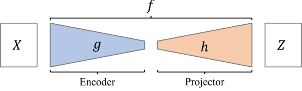
Figure 7: A schematic diagram of the architecture used by Joint Embedding methods which include VICReg, and Barlow Twins

In Figure 8, we demonstrate that our model’s performance plateaus at a much smaller projector dimension. This serves as empirical evidence supporting our algorithm as a robust choice for a range of scenarios.

Figure 8: Performance saturation in our model occurs at a much smaller projector size compared to VICReg and Barlow Twins, demonstrating its robustness.

H.2 Understanding Long-Term Convergence

A key insight from our learning curves in Figure 9 and Figure 10 is that the performance variation observed at 1000 epochs is largely a function of noise in early optimization stages. All models seem to follow similar convergence trends, underscoring that the performance differences are not indicative of intrinsic model superiority.

Figure 9: Learning curves for CIFAR-10 showing that the performance of models after 1000 epochs is influenced by noise in early optimization, with all models converging similarly.

Figure 10: Learning curves for CIFAR-100 emphasizing the role of early optimization noise in the performance after 1000 epochs, highlighting the similar convergence of all models.

Appendix I Reproducibility

In this section, we give further detail to allow readers to reproduce the results in the paper.

I.1 Code

We make code for the Stochastic CCA and Stochastic Deep CCA experiments available in the attached zip file. We will make this available as a public Github repository.

I.2 Computer Resources

Each of the four types of experiment required slightly different resources due to the relative scale of the problems.

Experiment	CPU/GPU Resources
Stochastic CCA	NVIDIA GeForce RTX 2080 Ti
Deep CCA	NVIDIA GeForce RTX 2080 Ti
Deep MCCA	NVIDIA GeForce RTX 2080 Ti
Stochastic PLS	NVIDIA GeForce GTX 1650 Ti
SSL	4-8 NVIDIA GeForce RTX 2080 Ti, Quadro RTX 8000
	Quadro RTX 6000, or NVIDIA GeForce GTX 1080 Ti GPU devices

Table 2: Computer resources for each experiment type

I.3 Further Experiment Details

In this section, we give further details regarding the including descriptions of the metrics and parameter search.

I.3.1 Stochastic CCA

Parameters: For each method, we searched over a hyperparameter grid using Biewald (2020).

Parameter	Values
minibatch size	5,20,50,100
components	5
epochs	1
seed	1, 2, 3, 4, 5
lr	0.01, 0.001, 0.0001
$\gamma$	0.01,0.1,1,10

I.3.2 Deep CCA

Further details: As in Wang et al. (2015b), we used multilayer perceptrons with two hidden layers with size 800 and an output layer of 50 with ReLU activations. We train for 20 epochs.

Parameters: For each method, we searched over a hyperparameter grid using Biewald (2020).

Parameter	Values
minibatch size	100, 50, 20
lr	1e-3, 1e-4, 1e-5
$\rho$	0.6, 0.8, 0.9
epochs	50

I.3.3 Deep MCCA

Parameters: For each method, we searched over a hyperparameter grid using Biewald (2020).

Parameter	Values
minibatch size	5,10,20,50,100,200
components	50
epochs	100
lr	0.01, 0.001, 0.0001, 0.00001

I.3.4 UK Biobank PLS

Partial Least Squares

Following section 2, we can combine equations 59 and 6 with $\alpha_{i}=1\forall i$ in order to write Partial Least Squares as a Generalized Eigenvalue Problem:

$$A=\begin{pmatrix}0&\mathrm{Cov}(X^{(1)},X^{(2)})\\ \mathrm{Cov}(X^{(2)},X^{(1)})&0\end{pmatrix},\quad B=\begin{pmatrix}I_{D_{1}}&0\\ 0&I_{D_{2}}\end{pmatrix},\quad u=\begin{pmatrix}u^{(1)}\\ u^{(2)}\end{pmatrix}.$$ (59)

Note that since $B$ is an Identity matrix by construction, we do not need to make stochastic approximations of $B$ during optimization.

Further details: The UK BioBank data consisted of real-valued continuous brain volumes and ordinal, integer genetic variants. We used pre-processed (using FreeSurfer (Fischl, 2012)) grey-matter volumes for 66 cortical (Desikan-Killiany atlas) and 16 subcortical brain regions and 582,565 autosomal genetic variants. The affects of age, age squared, intracranial volume, sex, and the first 20 genetic principal components for population structure were removed from the brain features using linear regression to account for any confounding effects. Each brain ROI was normalized by removing the mean and dividing the standard deviation. We processed the genetics data using PLINK (Purcell et al., 2007) keeping genetic variants with a minor allele frequency of at least 1% and a maximum missingness rate of 2%. We used mean imputation to fill in missing values and centered each variant.

To generate measures of genetic disease risk, we calculated polygenic risk scores using PRSice (Euesden et al., 2014). We calculated scores, with a p-value threshold of 0.05, using GWAS summary statistics for the following diseases; Alzheimer’s (Lambert et al., 2013), Schizophrenia (Trubetskoy et al., 2022), Bipolar (Mullins et al., 2021), ADHD (Demontis et al., 2023), ALS (van Rheenen et al., 2021), Parkinson’s (Nalls et al., 2019), and Epilepsy (International League Against Epilepsy Consortium on Complex Epilepsies, 2018), using the referenced GWAS studies.

The GEP-EY PLS analysis was trained for 100 epochs using a learning rate of 0.0001 with a minibatch size of 500.

I.3.5 Self-Supervised Learning

In this section, we provide a comprehensive overview of the experimental settings and configurations used in our self-supervised experiments.

As stated before, we use the standard setup from solo-learn’s pretraining scripts. For the backbone network, we use ResNet-18. The projector network consists of hidden dimensions and output dimensions both set to 2048. We employ the LARS optimizer with a learning rate of 0.3 for the backbone and 0.1 for the classifier. The batch size is set to 256, and weight decay is set to $1\times 10^{-4}$. Additional optimizer parameters include clip_lr set to True, $\eta$ set to 0.02, and exclude_bias_n_norm set to True. The learning rate scheduler used is a warmup cosine scheduler. The models are trained for 1000 epochs. The model’s calculations are performed with a numerical precision of 16 bits.

VICReg and Barlow Twins: Both models employ similar data augmentations, specified in Tables 3 and 4. In table 3 we show the shared augmentations while in table 4 we show the differences. Note that Barlow Twins uses two different augmentations with 50% probability each.

Augmentation	Parameters
ColorJitter	brightness = 0.4, contrast = 0.4, saturation = 0.2, hue = 0.1, prob = 0.8
Grayscale	prob = 0.2
HorizontalFlip	prob = 0.5
CropSize	32

Table 3: Shared augmentations for VICReg and Barlow Twins

Augmentation	VICReg	Barlow Twins (crop 1)	Barlow Twins (crop 2)
RandomResizedCrop	Yes	Yes	Yes
crop min scale	0.2	0.08	0.08
crop max scale	1.0	1.0	1.0
Solarization	Yes	No	Yes
	prob = 0.1	prob = 0.0	prob = 0.2
NumCrops	2	1	1

Table 4: Different augmentations for VICReg and Barlow Twins

I.4 PyTorch Pseudo-Code: Unifying the Algorithms under the Generalized Eigenproblem (GEP) Framework

In this work, we introduce three distinct algorithms: DMCCA-EY, PLS-EY, and SSL-EY. Despite their apparent differences, they are all specialized instances of a generalized eigenproblem (GEP). All these algorithms maximize the objective function outlined in Proposition 3.1, making them special cases of our main contribution.

Algorithm 2 gives a general loss for DCCA and DMCCA. Algorithm 3 shows how we can adapt the loss function for stochastic PLS problems. Algorithm 4 gives a generic SSL loss.

def DMCCA_EY(views, views_prime):

z = encode(views) # Encode the views

z_prime = encode(views_prime) # Encode the prime views

A, B, B_prime = torch.zeros(z[0].shape[1], z[0].shape[1]), torch.zeros(z[0].shape[1], z[0].shape[1]), torch.zeros(z[0].shape[1], z[0].shape[1]) # Initialize matrices

for zi, zj in all_pairs(z):

A += get_cross_covariance(zi, zj) # Compute cross-covariance

B += get_auto_covariance(zi) # Compute auto-covariance

for zi in z_prime:

B_prime += get_auto_covariance(zi) # Compute auto-covariance for prime views

A, B, B_prime = A / len(z), B / len(z), B_prime / len(z_prime) # Normalize matrices

return -torch.trace(2 * A - B @ B_prime) # Calculate loss

Algorithm 2 DMCCA-EY Loss Function in Python

def PLS_EY(views):

z, weights = encode_and_weights(views) # Encode the views and get weights

A, B = torch.zeros(z[0].shape[1], z[0].shape[1]), torch.zeros(weights[0].shape[1], weights[0].shape[1]) # Initialize matrices

for zi, zj in all_pairs(z):

A += cross_covariance_PLS(zi, zj) # Compute cross-covariance for PLS

for wi in weights:

B += auto_covariance_weights_PLS(wi) # Compute auto-covariance for PLS

A, B = A / len(z), B / len(weights) # Normalize matrices

return -torch.trace(2 * A - B @ B) # Calculate loss

Algorithm 3 PLS-EY Loss Function in Python

def SSL_EY(views, views_prime):

z = encode(views) # Encode the views

z_prime = encode(views_prime) # Encode the prime views

A, B, B_prime = torch.zeros(z[0].shape[1], z[0].shape[1]), torch.zeros(z[0].shape[1], z[0].shape[1]), torch.zeros(z[0].shape[1], z[0].shape[1]) # Initialize matrices

for zi, zj in all_pairs(z):

A += get_cross_covariance(zi, zj) # Compute cross-covariance

B += get_auto_covariance(zi) # Compute auto-covariance

for zi in z_prime:

B_prime += get_auto_covariance(zi) # Compute auto-covariance for prime views

A, B, B_prime = A / len(z), B / len(z), B_prime / len(z_prime) # Normalize matrices

Algorithm 4 SSL-EY Loss Function in Python

I.4.1 solo-learn adaptation

The version of SSL-EY in algorithm 5 is designed to integrate seamlessly into solo-learn, offering support for distributed training.

# Define the SSL-EY loss function

# Input: Projected features from two views

def SSL_EY(z1, z2):

# Get the minibatch size and feature dimension

N, D = z1.size()

# Compute the covariance matrix from the concatenated features

C = torch.cov(torch.hstack((z1, z2)).T)

# Average the covariance matrix across all processes if distributed training is enabled

if dist.is_available() and dist.is_initialized():

dist.all_reduce(C)

world_size = dist.get_world_size()

C /= world_size

# Extract symmetric and anti-symmetric blocks of C

A = C[:D, D:] + C[D:, :D]

B = C[:D, :D] + C[D:, D:]

# Return the SSL-EY loss value

return -torch.trace(2 * A - B @ B)

Algorithm 5 Solo-Learn Loss function for distributed SSL-EY in Python

References

• Altmann et al. (2023) Andre Altmann, Ana C Lawry Aquila, Neda Jahanshad, Paul M Thompson, and Marco Lorenzi. Tackling the dimensions in imaging genetics with CLUB-PLS. arXiv preprint arXiv:2309.07352, 2023.
• Andrew et al. (2013) Galen Andrew, Raman Arora, Jeff Bilmes, and Karen Livescu. Deep canonical correlation analysis. In International conference on machine learning, pp. 1247–1255. PMLR, 2013.
• Arora et al. (2012) Raman Arora, Andrew Cotter, Karen Livescu, and Nathan Srebro. Stochastic optimization for PCA and PLS. In 2012 50th Annual Allerton Conference on Communication, Control, and Computing (Allerton), pp.  861–868. IEEE, 2012.
• Balestriero & LeCun (2022) Randall Balestriero and Yann LeCun. Contrastive and non-contrastive self-supervised learning recover global and local spectral embedding methods. arXiv preprint arXiv:2205.11508, 2022.
• Balestriero et al. (2023) Randall Balestriero, Mark Ibrahim, Vlad Sobal, Ari Morcos, Shashank Shekhar, Tom Goldstein, Florian Bordes, Adrien Bardes, Gregoire Mialon, Yuandong Tian, et al. A cookbook of self-supervised learning. arXiv preprint arXiv:2304.12210, 2023.
• Bardes et al. (2021) Adrien Bardes, Jean Ponce, and Yann LeCun. Vicreg: Variance-invariance-covariance regularization for self-supervised learning. arXiv preprint arXiv:2105.04906, 2021.
• Benton et al. (2017) Adrian Benton, Huda Khayrallah, Biman Gujral, Dee Ann Reisinger, Sheng Zhang, and Raman Arora. Deep generalized canonical correlation analysis. arXiv preprint arXiv:1702.02519, 2017.
• Bhatia (1997) Rajendra Bhatia. Matrix Analysis, volume 169 of Graduate Texts in Mathematics. Springer, New York, NY, 1997. ISBN 978-1-4612-6857-4 978-1-4612-0653-8. doi: 10.1007/978-1-4612-0653-8. URL http://link.springer.com/10.1007/978-1-4612-0653-8.
• Biewald (2020) Lukas Biewald. Experiment tracking with weights and biases, 2020. URL https://www.wandb.com/. Software available from wandb.com.
• Borga (1998) Magnus Borga. Learning Multidimensional Signal Processing. PhD thesis, 1998. URL http://urn.kb.se/resolve?urn=urn:nbn:se:liu:diva-54341. Publisher: Linköping University Electronic Press.
• Carlsson (2021) Marcus Carlsson. von Neumann’s trace inequality for Hilbert–Schmidt operators. Expositiones Mathematicae, 39(1):149–157, March 2021. ISSN 0723-0869. doi: 10.1016/j.exmath.2020.05.001. URL https://www.sciencedirect.com/science/article/pii/S0723086920300220.
• Chang et al. (2018) Xiaobin Chang, Tao Xiang, and Timothy M Hospedales. Scalable and effective deep CCA via soft decorrelation. In Proceedings of the IEEE Conference on Computer Vision and Pattern Recognition, pp.  1488–1497, 2018.
• Chapman et al. (2022) James Chapman, Ana Lawry Aguila, and Lennie Wells. A generalized eigengame with extensions to multiview representation learning. arXiv preprint arXiv:2211.11323, 2022.
• Chen et al. (2019) Zhehui Chen, Xingguo Li, Lin Yang, Jarvis Haupt, and Tuo Zhao. On constrained nonconvex stochastic optimization: A case study for generalized eigenvalue decomposition. In The 22nd International Conference on Artificial Intelligence and Statistics, pp.  916–925. PMLR, 2019.
• Da Costa et al. (2022) Victor Guilherme Turrisi Da Costa, Enrico Fini, Moin Nabi, Nicu Sebe, and Elisa Ricci. solo-learn: A library of self-supervised methods for visual representation learning. J. Mach. Learn. Res., 23(56):1–6, 2022.
• Demontis et al. (2023) Ditte Demontis, G Bragi Walters, Georgios Athanasiadis, Raymond Walters, Karen Therrien, Trine Tollerup Nielsen, Leila Farajzadeh, Georgios Voloudakis, Jaroslav Bendl, Biau Zeng, Wen Zhang, Jakob Grove, Thomas D Als, Jinjie Duan, F Kyle Satterstrom, Jonas Bybjerg-Grauholm, Marie Bækved-Hansen, Olafur O Gudmundsson, Sigurdur H Magnusson, Gisli Baldursson, Katrin Davidsdottir, Gyda S Haraldsdottir, Esben Agerbo, Gabriel E Hoffman, Søren Dalsgaard, Joanna Martin, Marta Ribasés, Dorret I Boomsma, Maria Soler Artigas, Nina Roth Mota, Daniel Howrigan, Sarah E Medland, Tetyana Zayats, Veera M Rajagopal, ADHD Working Group of the Psychiatric Genomics Consortium, iPSYCH-Broad Consortium, Merete Nordentoft, Ole Mors, David M Hougaard, Preben Bo Mortensen, Mark J Daly, Stephen V Faraone, Hreinn Stefansson, Panos Roussos, Barbara Franke, Thomas Werge, Benjamin M Neale, Kari Stefansson, and Anders D Børglum. Genome-wide analyses of ADHD identify 27 risk loci, refine the genetic architecture and implicate several cognitive domains. Nat. Genet., 55(2):198–208, February 2023.
• Euesden et al. (2014) Jack Euesden, Cathryn M. Lewis, and Paul F. O’Reilly. PRSice: Polygenic Risk Score software. Bioinformatics, 31(9):1466–1468, 12 2014. ISSN 1367-4803. doi: 10.1093/bioinformatics/btu848. URL https://doi.org/10.1093/bioinformatics/btu848.
• Fischl (2012) Bruce Fischl. FreeSurfer. Neuroimage, 62(2):774–781, August 2012.
• Ge et al. (2015) Rong Ge, Furong Huang, Chi Jin, and Yang Yuan. Escaping from saddle points — online stochastic gradient for tensor decomposition, 2015.
• Ge et al. (2017) Rong Ge, Chi Jin, and Yi Zheng. No Spurious Local Minima in Nonconvex Low Rank Problems: A Unified Geometric Analysis. In Proceedings of the 34th International Conference on Machine Learning, pp.  1233–1242. PMLR, July 2017. URL https://proceedings.mlr.press/v70/ge17a.html. ISSN: 2640-3498.
• Gemp et al. (2021) Ian Gemp, Brian McWilliams, Claire Vernade, and Thore Graepel. Eigengame unloaded: When playing games is better than optimizing, 2021.
• Gemp et al. (2022) Ian Gemp, Charlie Chen, and Brian McWilliams. The generalized eigenvalue problem as a nash equilibrium. arXiv preprint arXiv:2206.04993, 2022.
• Gemp et al. (2020) Ian M. Gemp, Brian McWilliams, Claire Vernade, and Thore Graepel. EigenGame: PCA as a Nash Equilibrium. CoRR, abs/2010.00554, 2020. URL https://arxiv.org/abs/2010.00554.
• Haemers (1995) Willem H. Haemers. Interlacing eigenvalues and graphs. Linear Algebra and its Applications, 226-228:593–616, September 1995. ISSN 00243795. doi: 10.1016/0024-3795(95)00199-2. URL https://linkinghub.elsevier.com/retrieve/pii/0024379595001992.
• Hotelling (1933) Harold Hotelling. Analysis of a complex of statistical variables into principal components. Journal of educational psychology, 24(6):417, 1933.
• Hotelling (1992) Harold Hotelling. Relations between two sets of variates. In Breakthroughs in statistics, pp.  162–190. Springer, 1992.
• ICML (2023) ICML. ICML 2023, 2023. URL https://icml.cc/Conferences/2023/Test-of-Time.
• International League Against Epilepsy Consortium on Complex Epilepsies (2018) International League Against Epilepsy Consortium on Complex Epilepsies. Genome-wide mega-analysis identifies 16 loci and highlights diverse biological mechanisms in the common epilepsies. Nat. Commun., 9(1):5269, December 2018.
• Jing et al. (2021) Li Jing, Pascal Vincent, Yann LeCun, and Yuandong Tian. Understanding dimensional collapse in contrastive self-supervised learning. arXiv preprint arXiv:2110.09348, 2021.
• Lambert et al. (2013) J C Lambert, C A Ibrahim-Verbaas, D Harold, A C Naj, R Sims, C Bellenguez, A L DeStafano, J C Bis, G W Beecham, B Grenier-Boley, G Russo, T A Thorton-Wells, N Jones, A V Smith, V Chouraki, C Thomas, M A Ikram, D Zelenika, B N Vardarajan, Y Kamatani, C F Lin, A Gerrish, H Schmidt, B Kunkle, M L Dunstan, A Ruiz, M T Bihoreau, S H Choi, C Reitz, F Pasquier, C Cruchaga, D Craig, N Amin, C Berr, O L Lopez, P L De Jager, V Deramecourt, J A Johnston, D Evans, S Lovestone, L Letenneur, F J Morón, D C Rubinsztein, G Eiriksdottir, K Sleegers, A M Goate, N Fiévet, M W Huentelman, M Gill, K Brown, M I Kamboh, L Keller, P Barberger-Gateau, B McGuiness, E B Larson, R Green, A J Myers, C Dufouil, S Todd, D Wallon, S Love, E Rogaeva, J Gallacher, P St George-Hyslop, J Clarimon, A Lleo, A Bayer, D W Tsuang, L Yu, M Tsolaki, P Bossù, G Spalletta, P Proitsi, J Collinge, S Sorbi, F Sanchez-Garcia, N C Fox, J Hardy, M C Deniz Naranjo, P Bosco, R Clarke, C Brayne, D Galimberti, M Mancuso, F Matthews, European Alzheimer’s Disease Initiative (EADI), Genetic and Environmental Risk in Alzheimer’s Disease, Alzheimer’s Disease Genetic Consortium, Cohorts for Heart and Aging Research in Genomic Epidemiology, S Moebus, P Mecocci, M Del Zompo, W Maier, H Hampel, A Pilotto, M Bullido, F Panza, P Caffarra, B Nacmias, J R Gilbert, M Mayhaus, L Lannefelt, H Hakonarson, S Pichler, M M Carrasquillo, M Ingelsson, D Beekly, V Alvarez, F Zou, O Valladares, S G Younkin, E Coto, K L Hamilton-Nelson, W Gu, C Razquin, P Pastor, I Mateo, M J Owen, K M Faber, P V Jonsson, O Combarros, M C O’Donovan, L B Cantwell, H Soininen, D Blacker, S Mead, T H Mosley, Jr, D A Bennett, T B Harris, L Fratiglioni, C Holmes, R F de Bruijn, P Passmore, T J Montine, K Bettens, J I Rotter, A Brice, K Morgan, T M Foroud, W A Kukull, D Hannequin, J F Powell, M A Nalls, K Ritchie, K L Lunetta, J S Kauwe, E Boerwinkle, M Riemenschneider, M Boada, M Hiltuenen, E R Martin, R Schmidt, D Rujescu, L S Wang, J F Dartigues, R Mayeux, C Tzourio, A Hofman, M M Nöthen, C Graff, B M Psaty, L Jones, J L Haines, P A Holmans, M Lathrop, M A Pericak-Vance, L J Launer, L A Farrer, C M van Duijn, C Van Broeckhoven, V Moskvina, S Seshadri, J Williams, G D Schellenberg, and P Amouyel. Meta-analysis of 74,046 individuals identifies 11 new susceptibility loci for alzheimer’s disease. Nat. Genet., 45(12):1452–1458, December 2013.
• Lorenzi et al. (2017) Marco Lorenzi, Boris Gutman, Paul M Thompson, Daniel C Alexander, Sebastien Ourselin, and Andre Altmann. Secure multivariate large-scale multi-centric analysis through on-line learning: an imaging genetics case study. In 12th International Symposium on Medical Information Processing and Analysis, volume 10160, pp.  347–353. SPIE, 2017.
• Lorenzi et al. (2018) Marco Lorenzi, Andre Altmann, Boris Gutman, Selina Wray, Charles Arber, Derrek D Hibar, Neda J Jahanshad, Jonathan Schott, Daniel Alexander, Paul M. Thompson, and Sébastien Ourselin. Susceptibility of brain atrophy to TRIB3 in Alzheimer’s disease, evidence from functional prioritization in imaging genetics. Proceedings of the National Academy of Sciences of the United States of America, 115(12):3162–3167, 2018. doi: 10.1073/pnas.1706100115. URL https://hal.science/hal-01756811.
• Ma et al. (2023) Jiajun Ma, Tianyang Hu, and Wenjia Wang. Deciphering the projection head: Representation evaluation self-supervised learning. arXiv preprint arXiv:2301.12189, 2023.
• Meng et al. (2021) Zihang Meng, Rudrasis Chakraborty, and Vikas Singh. An online riemannian PCA for stochastic canonical correlation analysis. Advances in Neural Information Processing Systems, 34:14056–14068, 2021.
• Mihalik et al. (2022) Agoston Mihalik, James Chapman, Rick A. Adams, Nils R. Winter, Fabio S. Ferreira, John Shawe-Taylor, and Janaina Mourão-Miranda. Canonical Correlation Analysis and Partial Least Squares for identifying brain-behaviour associations: a tutorial and a comparative study. Biological Psychiatry: Cognitive Neuroscience and Neuroimaging, August 2022. ISSN 2451-9022. doi: 10.1016/j.bpsc.2022.07.012. URL https://www.sciencedirect.com/science/article/pii/S2451902222001859.
• Mills-Curran (1988) William C Mills-Curran. Calculation of eigenvector derivatives for structures with repeated eigenvalues. AIAA journal, 26(7):867–871, 1988.
• Mullins et al. (2021) Niamh Mullins, Andreas J Forstner, Kevin S O’Connell, Brandon Coombes, Jonathan R I Coleman, Zhen Qiao, Thomas D Als, Tim B Bigdeli, Sigrid Børte, Julien Bryois, Alexander W Charney, Ole Kristian Drange, Michael J Gandal, Saskia P Hagenaars, Masashi Ikeda, Nolan Kamitaki, Minsoo Kim, Kristi Krebs, Georgia Panagiotaropoulou, Brian M Schilder, Laura G Sloofman, Stacy Steinberg, Vassily Trubetskoy, Bendik S Winsvold, Hong-Hee Won, Liliya Abramova, Kristina Adorjan, Esben Agerbo, Mariam Al Eissa, Diego Albani, Ney Alliey-Rodriguez, Adebayo Anjorin, Verneri Antilla, Anastasia Antoniou, Swapnil Awasthi, Ji Hyun Baek, Marie Bækvad-Hansen, Nicholas Bass, Michael Bauer, Eva C Beins, Sarah E Bergen, Armin Birner, Carsten Bøcker Pedersen, Erlend Bøen, Marco P Boks, Rosa Bosch, Murielle Brum, Ben M Brumpton, Nathalie Brunkhorst-Kanaan, Monika Budde, Jonas Bybjerg-Grauholm, William Byerley, Murray Cairns, Miquel Casas, Pablo Cervantes, Toni-Kim Clarke, Cristiana Cruceanu, Alfredo Cuellar-Barboza, Julie Cunningham, David Curtis, Piotr M Czerski, Anders M Dale, Nina Dalkner, Friederike S David, Franziska Degenhardt, Srdjan Djurovic, Amanda L Dobbyn, Athanassios Douzenis, Torbjørn Elvsåshagen, Valentina Escott-Price, I Nicol Ferrier, Alessia Fiorentino, Tatiana M Foroud, Liz Forty, Josef Frank, Oleksandr Frei, Nelson B Freimer, Louise Frisén, Katrin Gade, Julie Garnham, Joel Gelernter, Marianne Giørtz Pedersen, Ian R Gizer, Scott D Gordon, Katherine Gordon-Smith, Tiffany A Greenwood, Jakob Grove, José Guzman-Parra, Kyooseob Ha, Magnus Haraldsson, Martin Hautzinger, Urs Heilbronner, Dennis Hellgren, Stefan Herms, Per Hoffmann, Peter A Holmans, Laura Huckins, Stéphane Jamain, Jessica S Johnson, Janos L Kalman, Yoichiro Kamatani, James L Kennedy, Sarah Kittel-Schneider, James A Knowles, Manolis Kogevinas, Maria Koromina, Thorsten M Kranz, Henry R Kranzler, Michiaki Kubo, Ralph Kupka, Steven A Kushner, Catharina Lavebratt, Jacob Lawrence, Markus Leber, Heon-Jeong Lee, Phil H Lee, Shawn E Levy, Catrin Lewis, Calwing Liao, Susanne Lucae, Martin Lundberg, Donald J MacIntyre, Sigurdur H Magnusson, Wolfgang Maier, Adam Maihofer, Dolores Malaspina, Eirini Maratou, Lina Martinsson, Manuel Mattheisen, Steven A McCarroll, Nathaniel W McGregor, Peter McGuffin, James D McKay, Helena Medeiros, Sarah E Medland, Vincent Millischer, Grant W Montgomery, Jennifer L Moran, Derek W Morris, Thomas W Mühleisen, Niamh O’Brien, Claire O’Donovan, Loes M Olde Loohuis, Lilijana Oruc, Sergi Papiol, Antonio F Pardiñas, Amy Perry, Andrea Pfennig, Evgenia Porichi, James B Potash, Digby Quested, Towfique Raj, Mark H Rapaport, J Raymond DePaulo, Eline J Regeer, John P Rice, Fabio Rivas, Margarita Rivera, Julian Roth, Panos Roussos, Douglas M Ruderfer, Cristina Sánchez-Mora, Eva C Schulte, Fanny Senner, Sally Sharp, Paul D Shilling, Engilbert Sigurdsson, Lea Sirignano, Claire Slaney, Olav B Smeland, Daniel J Smith, Janet L Sobell, Christine Søholm Hansen, Maria Soler Artigas, Anne T Spijker, Dan J Stein, John S Strauss, Beata Swikatkowska, Chikashi Terao, Thorgeir E Thorgeirsson, Claudio Toma, Paul Tooney, Evangelia-Eirini Tsermpini, Marquis P Vawter, Helmut Vedder, James T R Walters, Stephanie H Witt, Simon Xi, Wei Xu, Jessica Mei Kay Yang, Allan H Young, Hannah Young, Peter P Zandi, Hang Zhou, Lea Zillich, HUNT All-In Psychiatry, Rolf Adolfsson, Ingrid Agartz, Martin Alda, Lars Alfredsson, Gulja Babadjanova, Lena Backlund, Bernhard T Baune, Frank Bellivier, Susanne Bengesser, Wade H Berrettini, Douglas H R Blackwood, Michael Boehnke, Anders D Børglum, Gerome Breen, Vaughan J Carr, Stanley Catts, Aiden Corvin, Nicholas Craddock, Udo Dannlowski, Dimitris Dikeos, Tõnu Esko, Bruno Etain, Panagiotis Ferentinos, Mark Frye, Janice M Fullerton, Micha Gawlik, Elliot S Gershon, Fernando S Goes, Melissa J Green, Maria Grigoroiu-Serbanescu, Joanna Hauser, Frans Henskens, Jan Hillert, Kyung Sue Hong, David M Hougaard, Christina M Hultman, Kristian Hveem, Nakao Iwata, Assen V Jablensky, Ian Jones, Lisa A Jones, René S Kahn, John R Kelsoe, George Kirov, Mikael Landén, Marion Leboyer, Cathryn M Lewis, Qingqin S Li, Jolanta Lissowska, Christine Lochner, Carmel Loughland, Nicholas G Martin, Carol A Mathews, Fermin Mayoral, Susan L McElroy, Andrew M McIntosh, Francis J McMahon, Ingrid Melle, Patricia Michie, Lili Milani, Philip B Mitchell, Gunnar Morken, Ole Mors, Preben Bo Mortensen, Bryan Mowry, Bertram Müller-Myhsok, Richard M Myers, Benjamin M Neale, Caroline M Nievergelt, Merete Nordentoft, Markus M Nöthen, Michael C O’Donovan, Ketil J Oedegaard, Tomas Olsson, Michael J Owen, Sara A Paciga, Chris Pantelis, Carlos Pato, Michele T Pato, George P Patrinos, Roy H Perlis, Danielle Posthuma, Josep Antoni Ramos-Quiroga, Andreas Reif, Eva Z Reininghaus, Marta Ribasés, Marcella Rietschel, Stephan Ripke, Guy A Rouleau, Takeo Saito, Ulrich Schall, Martin Schalling, Peter R Schofield, Thomas G Schulze, Laura J Scott, Rodney J Scott, Alessandro Serretti, Cynthia Shannon Weickert, Jordan W Smoller, Hreinn Stefansson, Kari Stefansson, Eystein Stordal, Fabian Streit, Patrick F Sullivan, Gustavo Turecki, Arne E Vaaler, Eduard Vieta, John B Vincent, Irwin D Waldman, Thomas W Weickert, Thomas Werge, Naomi R Wray, John-Anker Zwart, Joanna M Biernacka, John I Nurnberger, Sven Cichon, Howard J Edenberg, Eli A Stahl, Andrew McQuillin, Arianna Di Florio, Roel A Ophoff, and Ole A Andreassen. Genome-wide association study of more than 40,000 bipolar disorder cases provides new insights into the underlying biology. Nat. Genet., 53(6):817–829, June 2021.
• Nalls et al. (2019) Mike A Nalls, Cornelis Blauwendraat, Costanza L Vallerga, Karl Heilbron, Sara Bandres-Ciga, Diana Chang, Manuela Tan, Demis A Kia, Alastair J Noyce, Angli Xue, Jose Bras, Emily Young, Rainer von Coelln, Javier Simón-Sánchez, Claudia Schulte, Manu Sharma, Lynne Krohn, Lasse Pihlstrøm, Ari Siitonen, Hirotaka Iwaki, Hampton Leonard, Faraz Faghri, J Raphael Gibbs, Dena G Hernandez, Sonja W Scholz, Juan A Botia, Maria Martinez, Jean-Christophe Corvol, Suzanne Lesage, Joseph Jankovic, Lisa M Shulman, Margaret Sutherland, Pentti Tienari, Kari Majamaa, Mathias Toft, Ole A Andreassen, Tushar Bangale, Alexis Brice, Jian Yang, Ziv Gan-Or, Thomas Gasser, Peter Heutink, Joshua M Shulman, Nicholas W Wood, David A Hinds, John A Hardy, Huw R Morris, Jacob Gratten, Peter M Visscher, Robert R Graham, Andrew B Singleton, 23andMe Research Team, System Genomics of Parkinson’s Disease Consortium, and International Parkinson’s Disease Genomics Consortium. Identification of novel risk loci, causal insights, and heritable risk for parkinson’s disease: a meta-analysis of genome-wide association studies. Lancet Neurol., 18(12):1091–1102, December 2019.
• Nielsen (2002) Allan Aasbjerg Nielsen. Multiset canonical correlations analysis and multispectral, truly multitemporal remote sensing data. IEEE transactions on image processing, 11(3):293–305, 2002.
• Purcell et al. (2007) Shaun Purcell, Benjamin Neale, Kathe Todd-Brown, Lori Thomas, Manuel A R Ferreira, David Bender, Julian Maller, Pamela Sklar, Paul I W de Bakker, Mark J Daly, and Pak C Sham. PLINK: a tool set for whole-genome association and population-based linkage analyses. Am. J. Hum. Genet., 81(3):559–575, September 2007.
• Somandepalli et al. (2019) Krishna Somandepalli, Naveen Kumar, Ruchir Travadi, and Shrikanth Narayanan. Multimodal representation learning using deep multiset canonical correlation. arXiv preprint arXiv:1904.01775, 2019.
• Stewart & Sun (1990) G. W. Stewart and Ji-Guang Sun. Matrix Perturbation Theory. ACADEMIC PressINC, July 1990. ISBN 978-1-4933-0199-7. Google-Books-ID: bIYEogEACAAJ.
• Sudlow et al. (2015) Cathie Sudlow, John Gallacher, Naomi Allen, Valerie Beral, Paul Burton, John Danesh, Paul Downey, Paul Elliott, Jane Green, Martin Landray, et al. Uk biobank: an open access resource for identifying the causes of a wide range of complex diseases of middle and old age. PLoS medicine, 12(3):e1001779, 2015.
• Taquet et al. (2021) Maxime Taquet, Stephen M Smith, Anna K Prohl, Jurriaan M Peters, Simon K Warfield, Benoit Scherrer, and Paul J Harrison. A structural brain network of genetic vulnerability to psychiatric illness. Mol. Psychiatry, 26(6):2089–2100, June 2021.
• Tong et al. (2023) Shengbang Tong, Yubei Chen, Yi Ma, and Yann Lecun. EMP-SSL: rowards self-supervised learning in one training epoch. arXiv preprint arXiv:2304.03977, 2023.
• Trubetskoy et al. (2022) Vassily Trubetskoy, Antonio F Pardiñas, Ting Qi, Georgia Panagiotaropoulou, Swapnil Awasthi, Tim B Bigdeli, Julien Bryois, Chia-Yen Chen, Charlotte A Dennison, Lynsey S Hall, Max Lam, Kyoko Watanabe, Oleksandr Frei, Tian Ge, Janet C Harwood, Frank Koopmans, Sigurdur Magnusson, Alexander L Richards, Julia Sidorenko, Yang Wu, Jian Zeng, Jakob Grove, Minsoo Kim, Zhiqiang Li, Georgios Voloudakis, Wen Zhang, Mark Adams, Ingrid Agartz, Elizabeth G Atkinson, Esben Agerbo, Mariam Al Eissa, Margot Albus, Madeline Alexander, Behrooz Z Alizadeh, Köksal Alptekin, Thomas D Als, Farooq Amin, Volker Arolt, Manuel Arrojo, Lavinia Athanasiu, Maria Helena Azevedo, Silviu A Bacanu, Nicholas J Bass, Martin Begemann, Richard A Belliveau, Judit Bene, Beben Benyamin, Sarah E Bergen, Giuseppe Blasi, Julio Bobes, Stefano Bonassi, Alice Braun, Rodrigo Affonseca Bressan, Evelyn J Bromet, Richard Bruggeman, Peter F Buckley, Randy L Buckner, Jonas Bybjerg-Grauholm, Wiepke Cahn, Murray J Cairns, Monica E Calkins, Vaughan J Carr, David Castle, Stanley V Catts, Kimberley D Chambert, Raymond C K Chan, Boris Chaumette, Wei Cheng, Eric F C Cheung, Siow Ann Chong, David Cohen, Angèle Consoli, Quirino Cordeiro, Javier Costas, Charles Curtis, Michael Davidson, Kenneth L Davis, Lieuwe de Haan, Franziska Degenhardt, Lynn E DeLisi, Ditte Demontis, Faith Dickerson, Dimitris Dikeos, Timothy Dinan, Srdjan Djurovic, Jubao Duan, Giuseppe Ducci, Frank Dudbridge, Johan G Eriksson, Lourdes Fañanás, Stephen V Faraone, Alessia Fiorentino, Andreas Forstner, Josef Frank, Nelson B Freimer, Menachem Fromer, Alessandra Frustaci, Ary Gadelha, Giulio Genovese, Elliot S Gershon, Marianna Giannitelli, Ina Giegling, Paola Giusti-Rodríguez, Stephanie Godard, Jacqueline I Goldstein, Javier González Peñas, Ana González-Pinto, Srihari Gopal, Jacob Gratten, Michael F Green, Tiffany A Greenwood, Olivier Guillin, Sinan Gülöksüz, Raquel E Gur, Ruben C Gur, Blanca Gutiérrez, Eric Hahn, Hakon Hakonarson, Vahram Haroutunian, Annette M Hartmann, Carol Harvey, Caroline Hayward, Frans A Henskens, Stefan Herms, Per Hoffmann, Daniel P Howrigan, Masashi Ikeda, Conrad Iyegbe, Inge Joa, Antonio Julià, Anna K Kähler, Tony Kam-Thong, Yoichiro Kamatani, Sena Karachanak-Yankova, Oussama Kebir, Matthew C Keller, Brian J Kelly, Andrey Khrunin, Sung-Wan Kim, Janis Klovins, Nikolay Kondratiev, Bettina Konte, Julia Kraft, Michiaki Kubo, Vaidutis Kučinskas, Zita Ausrele Kučinskiene, Agung Kusumawardhani, Hana Kuzelova-Ptackova, Stefano Landi, Laura C Lazzeroni, Phil H Lee, Sophie E Legge, Douglas S Lehrer, Rebecca Lencer, Bernard Lerer, Miaoxin Li, Jeffrey Lieberman, Gregory A Light, Svetlana Limborska, Chih-Min Liu, Jouko Lönnqvist, Carmel M Loughland, Jan Lubinski, Jurjen J Luykx, Amy Lynham, Milan Macek, Jr, Andrew Mackinnon, Patrik K E Magnusson, Brion S Maher, Wolfgang Maier, Dolores Malaspina, Jacques Mallet, Stephen R Marder, Sara Marsal, Alicia R Martin, Lourdes Martorell, Manuel Mattheisen, Robert W McCarley, Colm McDonald, John J McGrath, Helena Medeiros, Sandra Meier, Bela Melegh, Ingrid Melle, Raquelle I Mesholam-Gately, Andres Metspalu, Patricia T Michie, Lili Milani, Vihra Milanova, Marina Mitjans, Espen Molden, Esther Molina, María Dolores Molto, Valeria Mondelli, Carmen Moreno, Christopher P Morley, Gerard Muntané, Kieran C Murphy, Inez Myin-Germeys, Igor Nenadić, Gerald Nestadt, Liene Nikitina-Zake, Cristiano Noto, Keith H Nuechterlein, Niamh Louise O’Brien, F Anthony O’Neill, Sang-Yun Oh, Ann Olincy, Vanessa Kiyomi Ota, Christos Pantelis, George N Papadimitriou, Mara Parellada, Tiina Paunio, Renata Pellegrino, Sathish Periyasamy, Diana O Perkins, Bruno Pfuhlmann, Olli Pietiläinen, Jonathan Pimm, David Porteous, John Powell, Diego Quattrone, Digby Quested, Allen D Radant, Antonio Rampino, Mark H Rapaport, Anna Rautanen, Abraham Reichenberg, Cheryl Roe, Joshua L Roffman, Julian Roth, Matthias Rothermundt, Bart P F Rutten, Safaa Saker-Delye, Veikko Salomaa, Julio Sanjuan, Marcos Leite Santoro, Adam Savitz, Ulrich Schall, Rodney J Scott, Larry J Seidman, Sally Isabel Sharp, Jianxin Shi, Larry J Siever, Engilbert Sigurdsson, Kang Sim, Nora Skarabis, Petr Slominsky, Hon-Cheong So, Janet L Sobell, Erik Söderman, Helen J Stain, Nils Eiel Steen, Agnes A Steixner-Kumar, Elisabeth Stögmann, William S Stone, Richard E Straub, Fabian Streit, Eric Strengman, T Scott Stroup, Mythily Subramaniam, Catherine A Sugar, Jaana Suvisaari, Dragan M Svrakic, Neal R Swerdlow, Jin P Szatkiewicz, Thi Minh Tam Ta, Atsushi Takahashi, Chikashi Terao, Florence Thibaut, Draga Toncheva, Paul A Tooney, Silvia Torretta, Sarah Tosato, Gian Battista Tura, Bruce I Turetsky, Alp Üçok, Arne Vaaler, Therese van Amelsvoort, Ruud van Winkel, Juha Veijola, John Waddington, Henrik Walter, Anna Waterreus, Bradley T Webb, Mark Weiser, Nigel M Williams, Stephanie H Witt, Brandon K Wormley, Jing Qin Wu, Zhida Xu, Robert Yolken, Clement C Zai, Wei Zhou, Feng Zhu, Fritz Zimprich, Eşref Cem Atbaşoğlu, Muhammad Ayub, Christian Benner, Alessandro Bertolino, Donald W Black, Nicholas J Bray, Gerome Breen, Nancy G Buccola, William F Byerley, Wei J Chen, C Robert Cloninger, Benedicto Crespo-Facorro, Gary Donohoe, Robert Freedman, Cherrie Galletly, Michael J Gandal, Massimo Gennarelli, David M Hougaard, Hai-Gwo Hwu, Assen V Jablensky, Steven A McCarroll, Jennifer L Moran, Ole Mors, Preben B Mortensen, Bertram Müller-Myhsok, Amanda L Neil, Merete Nordentoft, Michele T Pato, Tracey L Petryshen, Matti Pirinen, Ann E Pulver, Thomas G Schulze, Jeremy M Silverman, Jordan W Smoller, Eli A Stahl, Debby W Tsuang, Elisabet Vilella, Shi-Heng Wang, Shuhua Xu, Indonesia Schizophrenia Consortium, PsychENCODE, Psychosis Endophenotypes International Consortium, SynGO Consortium, Rolf Adolfsson, Celso Arango, Bernhard T Baune, Sintia Iole Belangero, Anders D Børglum, David Braff, Elvira Bramon, Joseph D Buxbaum, Dominique Campion, Jorge A Cervilla, Sven Cichon, David A Collier, Aiden Corvin, David Curtis, Marta Di Forti, Enrico Domenici, Hannelore Ehrenreich, Valentina Escott-Price, Tõnu Esko, Ayman H Fanous, Anna Gareeva, Micha Gawlik, Pablo V Gejman, Michael Gill, Stephen J Glatt, Vera Golimbet, Kyung Sue Hong, Christina M Hultman, Steven E Hyman, Nakao Iwata, Erik G Jönsson, René S Kahn, James L Kennedy, Elza Khusnutdinova, George Kirov, James A Knowles, Marie-Odile Krebs, Claudine Laurent-Levinson, Jimmy Lee, Todd Lencz, Douglas F Levinson, Qingqin S Li, Jianjun Liu, Anil K Malhotra, Dheeraj Malhotra, Andrew McIntosh, Andrew McQuillin, Paulo R Menezes, Vera A Morgan, Derek W Morris, Bryan J Mowry, Robin M Murray, Vishwajit Nimgaonkar, Markus M Nöthen, Roel A Ophoff, Sara A Paciga, Aarno Palotie, Carlos N Pato, Shengying Qin, Marcella Rietschel, Brien P Riley, Margarita Rivera, Dan Rujescu, Meram C Saka, Alan R Sanders, Sibylle G Schwab, Alessandro Serretti, Pak C Sham, Yongyong Shi, David St Clair, Hreinn Stefánsson, Kari Stefansson, Ming T Tsuang, Jim van Os, Marquis P Vawter, Daniel R Weinberger, Thomas Werge, Dieter B Wildenauer, Xin Yu, Weihua Yue, Peter A Holmans, Andrew J Pocklington, Panos Roussos, Evangelos Vassos, Matthijs Verhage, Peter M Visscher, Jian Yang, Danielle Posthuma, Ole A Andreassen, Kenneth S Kendler, Michael J Owen, Naomi R Wray, Mark J Daly, Hailiang Huang, Benjamin M Neale, Patrick F Sullivan, Stephan Ripke, James T R Walters, Michael C O’Donovan, and Schizophrenia Working Group of the Psychiatric Genomics Consortium. Mapping genomic loci implicates genes and synaptic biology in schizophrenia. Nature, 604(7906):502–508, April 2022.
• van Rheenen et al. (2021) Wouter van Rheenen, Rick A A van der Spek, Mark K Bakker, Joke J F A van Vugt, Paul J Hop, Ramona A J Zwamborn, Niek de Klein, Harm-Jan Westra, Olivier B Bakker, Patrick Deelen, Gemma Shireby, Eilis Hannon, Matthieu Moisse, Denis Baird, Restuadi Restuadi, Egor Dolzhenko, Annelot M Dekker, Klara Gawor, Henk-Jan Westeneng, Gijs H P Tazelaar, Kristel R van Eijk, Maarten Kooyman, Ross P Byrne, Mark Doherty, Mark Heverin, Ahmad Al Khleifat, Alfredo Iacoangeli, Aleksey Shatunov, Nicola Ticozzi, Johnathan Cooper-Knock, Bradley N Smith, Marta Gromicho, Siddharthan Chandran, Suvankar Pal, Karen E Morrison, Pamela J Shaw, John Hardy, Richard W Orrell, Michael Sendtner, Thomas Meyer, Nazli Başak, Anneke J van der Kooi, Antonia Ratti, Isabella Fogh, Cinzia Gellera, Giuseppe Lauria, Stefania Corti, Cristina Cereda, Daisy Sproviero, Sandra D’Alfonso, Gianni Sorarù, Gabriele Siciliano, Massimiliano Filosto, Alessandro Padovani, Adriano Chiò, Andrea Calvo, Cristina Moglia, Maura Brunetti, Antonio Canosa, Maurizio Grassano, Ettore Beghi, Elisabetta Pupillo, Giancarlo Logroscino, Beatrice Nefussy, Alma Osmanovic, Angelica Nordin, Yossef Lerner, Michal Zabari, Marc Gotkine, Robert H Baloh, Shaughn Bell, Patrick Vourc’h, Philippe Corcia, Philippe Couratier, Stéphanie Millecamps, Vincent Meininger, François Salachas, Jesus S Mora Pardina, Abdelilah Assialioui, Ricardo Rojas-García, Patrick A Dion, Jay P Ross, Albert C Ludolph, Jochen H Weishaupt, David Brenner, Axel Freischmidt, Gilbert Bensimon, Alexis Brice, Alexandra Durr, Christine A M Payan, Safa Saker-Delye, Nicholas W Wood, Simon Topp, Rosa Rademakers, Lukas Tittmann, Wolfgang Lieb, Andre Franke, Stephan Ripke, Alice Braun, Julia Kraft, David C Whiteman, Catherine M Olsen, Andre G Uitterlinden, Albert Hofman, Marcella Rietschel, Sven Cichon, Markus M Nöthen, Philippe Amouyel, SLALOM Consortium, PARALS Consortium, SLAGEN Consortium, SLAP Consortium, Bryan J Traynor, Andrew B Singleton, Miguel Mitne Neto, Ruben J Cauchi, Roel A Ophoff, Martina Wiedau-Pazos, Catherine Lomen-Hoerth, Vivianna M van Deerlin, Julian Grosskreutz, Annekathrin Roediger, Nayana Gaur, Alexander Jörk, Tabea Barthel, Erik Theele, Benjamin Ilse, Beatrice Stubendorff, Otto W Witte, Robert Steinbach, Christian A Hübner, Caroline Graff, Lev Brylev, Vera Fominykh, Vera Demeshonok, Anastasia Ataulina, Boris Rogelj, Blaž Koritnik, Janez Zidar, Metka Ravnik-Glavač, Damjan Glavač, Zorica Stević, Vivian Drory, Monica Povedano, Ian P Blair, Matthew C Kiernan, Beben Benyamin, Robert D Henderson, Sarah Furlong, Susan Mathers, Pamela A McCombe, Merrilee Needham, Shyuan T Ngo, Garth A Nicholson, Roger Pamphlett, Dominic B Rowe, Frederik J Steyn, Kelly L Williams, Karen A Mather, Perminder S Sachdev, Anjali K Henders, Leanne Wallace, Mamede de Carvalho, Susana Pinto, Susanne Petri, Markus Weber, Guy A Rouleau, Vincenzo Silani, Charles J Curtis, Gerome Breen, Jonathan D Glass, Robert H Brown, Jr, John E Landers, Christopher E Shaw, Peter M Andersen, Ewout J N Groen, Michael A van Es, R Jeroen Pasterkamp, Dongsheng Fan, Fleur C Garton, Allan F McRae, George Davey Smith, Tom R Gaunt, Michael A Eberle, Jonathan Mill, Russell L McLaughlin, Orla Hardiman, Kevin P Kenna, Naomi R Wray, Ellen Tsai, Heiko Runz, Lude Franke, Ammar Al-Chalabi, Philip Van Damme, Leonard H van den Berg, and Jan H Veldink. Common and rare variant association analyses in amyotrophic lateral sclerosis identify 15 risk loci with distinct genetic architectures and neuron-specific biology. Nat. Genet., 53(12):1636–1648, December 2021.
• Vinod (1976) Hrishikesh D Vinod. Canonical ridge and econometrics of joint production. Journal of econometrics, 4(2):147–166, 1976.
• Wang et al. (2015a) Weiran Wang, Raman Arora, Karen Livescu, and Jeff A Bilmes. Unsupervised learning of acoustic features via deep canonical correlation analysis. In 2015 IEEE International Conference on Acoustics, Speech and Signal Processing (ICASSP), pp.  4590–4594. IEEE, 2015a.
• Wang et al. (2015b) Weiran Wang, Raman Arora, Karen Livescu, and Nathan Srebro. Stochastic optimization for deep CCA via nonlinear orthogonal iterations. In 2015 53rd Annual Allerton Conference on Communication, Control, and Computing (Allerton), pp.  688–695. IEEE, 2015b.
• Witten & Tibshirani (2009) Daniela M Witten and Robert J Tibshirani. Extensions of sparse canonical correlation analysis with applications to genomic data. Statistical applications in genetics and molecular biology, 8(1), 2009.
• Wong et al. (2021) Hok Shing Wong, Li Wang, Raymond Chan, and Tieyong Zeng. Deep tensor CCA for multi-view learning. IEEE Transactions on Big Data, 8(6):1664–1677, 2021.
• Zbontar et al. (2021) Jure Zbontar, Li Jing, Ishan Misra, Yann LeCun, and Stéphane Deny. Barlow twins: Self-supervised learning via redundancy reduction. arXiv preprint arXiv:2103.03230, 2021.
• Édith Le Floch et al. (2012) Édith Le Floch, Vincent Guillemot, Vincent Frouin, Philippe Pinel, Christophe Lalanne, Laura Trinchera, Arthur Tenenhaus, Antonio Moreno, Monica Zilbovicius, Thomas Bourgeron, Stanislas Dehaene, Bertrand Thirion, Jean-Baptiste Poline, and Édouard Duchesnay. Significant correlation between a set of genetic polymorphisms and a functional brain network revealed by feature selection and sparse partial least squares. NeuroImage, 63(1):11–24, 2012. ISSN 1053-8119. doi: https://doi.org/10.1016/j.neuroimage.2012.06.061. URL https://www.sciencedirect.com/science/article/pii/S1053811912006775.